the Creative Commons Attribution 3.0 License.
the Creative Commons Attribution 3.0 License.
Assimilating solar-induced chlorophyll fluorescence into the terrestrial biosphere model BETHY-SCOPE v1.0: model description and information content
Alexander J. Norton
Peter J. Rayner
Ernest N. Koffi
Marko Scholze
The synthesis of model and observational information using data assimilation can improve our understanding of the terrestrial carbon cycle, a key component of the Earth's climate–carbon system. Here we provide a data assimilation framework for combining observations of solar-induced chlorophyll fluorescence (SIF) and a process-based model to improve estimates of terrestrial carbon uptake or gross primary production (GPP). We then quantify and assess the constraint SIF provides on the uncertainty in global GPP through model process parameters in an error propagation study. By incorporating 1 year of SIF observations from the GOSAT satellite, we find that the parametric uncertainty in global annual GPP is reduced by 73 % from ±19.0 to ±5.2 Pg C yr−1. This improvement is achieved through strong constraint of leaf growth processes and weak to moderate constraint of physiological parameters. We also find that the inclusion of uncertainty in shortwave down-radiation forcing has a net-zero effect on uncertainty in GPP when incorporated into the SIF assimilation framework. This study demonstrates the powerful capacity of SIF to reduce uncertainties in process-based model estimates of GPP and the potential for improving our predictive capability of this uncertain carbon flux.


The productivity of the terrestrial biosphere forms a key component of Earth's climate–carbon system. Estimates show that the terrestrial biosphere has removed about one quarter of all anthropogenic CO2 emissions, thus preventing additional climate warming (Ciais et al., 2013). Much of the interannual variability in atmospheric CO2 concentration is also driven by terrestrial productivity. Despite this significance, an understanding of the underlying mechanisms of terrestrial productivity is still lacking. This results in large uncertainties in predictions of terrestrial productivity and thus predictions of future atmospheric CO2 and temperature (Friedlingstein et al., 2006).
A key challenge is disaggregating the observable net CO2 flux into its component fluxes: gross primary production and ecosystem respiration. Gross primary production (GPP) is the rate of CO2 uptake through plant photosynthesis and the largest natural surface-to-atmosphere flux of carbon on Earth (Ciais et al., 2013). Estimating spatiotemporal patterns of GPP at the scales required for global change and modelling studies has proven difficult. This is primarily for two reasons: the complexity of the processes involved and the difficulty in observing those processes (Baldocchi et al., 2016; Schimel et al., 2015). Remote-sensing observations of solar-induced chlorophyll fluorescence (SIF) offer a novel constraint on GPP and the potential to partly address these two issues (Schimel et al., 2015).
At the leaf scale chlorophyll fluorescence is emitted from photosystems I and II during the light reactions of photosynthesis. These photosystems are pigment–protein complexes that form the reaction centres for converting light energy into chemical energy. It is in photosystem II (PSII) where photochemistry, the process initiating photosynthetic electron transport and leading to CO2 fixation, is initiated. The link between chlorophyll fluorescence and photochemistry is confounded by a third key process, however: heat dissipation, also termed non-photochemical quenching (NPQ). Both photochemistry and NPQ are regulated processes, responding to changing physiological and environmental conditions (Porcar-Castell et al., 2014). Changes in the rates of photochemistry and NPQ, and electron sinks other than CO2 fixation, lead to a non-trivial but direct link between chlorophyll fluorescence and photosynthetic rate (Flexas et al., 1999; Magney et al., 2017). Because chlorophyll fluorescence is tied in with these physiological processes, it has become a highly useful indicator of the physiological state of leaves (see reviews by Baker, 2008; Porcar-Castell et al., 2014).
At the canopy scale and beyond, the link appears simpler, exhibiting ecosystem-dependent linear relationships (Guanter et al., 2013). The slope of this linear relationship can change as the light-use efficiency of either SIF or GPP changes, for example due to water stress (Daumard et al., 2010) or changing light conditions (Yang et al., 2015). SIF also seems to outperform traditional remote-sensing methods, such as the Normalized Difference Vegetation Index (NDVI) and the Enhanced Vegetation Index (EVI), which use reflectance to derive vegetation indices, in tracking changes in GPP at this scale (Yang et al., 2015; Walther et al., 2016). This is in part because the SIF emission originates exclusively from plants; thus, the retrieval is not contaminated by background materials like soil or snow. It is expected, however, that complicating factors such as the retrieval wavelength, temporal scaling, chlorophyll content, three-dimensional canopy structure, and stress will also play a role in the GPP–SIF link (Damm et al., 2015; Guanter et al., 2012; Rossini et al., 2015; Zhang et al., 2016). Using high-resolution spectrometers onboard satellites, global maps of SIF have been produced. A number of existing (GOME-2, GOSAT, OCO-2, TROPOMI, SCHIAMACHY) and planned (FLEX, GEOCARB) satellite missions are capable of measuring SIF. Utilizing these remotely sensed SIF observations directly to track changes in GPP has already proven useful even without the addition of ancillary data or model information (Lee et al., 2013; Parazoo et al., 2013; Walther et al., 2016; Yang et al., 2015).
Data assimilation enables the use of observations and model information together to produce a best estimate of the state and function of the system. In the case of mechanistic models this is done by constraining the simulated processes and their parameters. Such an approach has been applied to terrestrial biosphere models to optimize model parameters and constrain the uncertainty in carbon flux estimates in a number of studies (see Kaminski et al., 2013; Koffi et al., 2013; Macbean et al., 2016; Peylin et al., 2016). The Carbon Cycle Data Assimilation System (CCDAS) is one such system, and it has incorporated observations such as atmospheric CO2 concentration and/or the fraction of absorbed photosynthetically active radiation (FAPAR), demonstrating the benefit of combining model and observations in a regularized approach (Rayner et al., 2005; Kaminski et al., 2012). The use of SIF observations within a data assimilation framework may provide a highly useful, complementary constraint on GPP. While one study by Parazoo et al. (2014) utilized SIF in a data assimilation system to redistribute multiple model estimates of GPP, no optimization of model process parameters was performed. Koffi et al. (2015) incorporated a mechanistic model for SIF into the CCDAS system and then conducted sensitivity tests and compared model-simulated SIF and observed SIF from GOSAT, demonstrating that the model is capable of incorporating the data. However, SIF has not yet been used on a global scale in a data assimilation system to optimize process parameters.
In this paper, we assess the ability of satellite SIF observations to constrain the parametric uncertainty in simulated GPP in a terrestrial biosphere model within a data assimilation system. This is termed an error propagation study and is similar in concept to an observing system simulation experiment or quantitative network design study (Hungershoefer et al., 2010; Kaminski et al., 2010; Koffi et al., 2013). Parameters and simulated GPP are therefore optimized only for their uncertainty and not for their absolute quantities. Considering that SIF is a novel observational constraint, this is an important first step toward a full assimilation of the data as it allows us to test whether an assimilation of SIF data will be beneficial for reducing uncertainty in GPP. This is performed by estimating the constraint that SIF provides on the uncertainty in model parameters and the parametric uncertainty in model-simulated GPP.
Under the linear Gaussian assumption, the uncertainty in a target quantity (here, GPP) following the assimilation of the measured data (here, SIF) is conditional only on the prior uncertainty, the uncertainty in the measured data and the sensitivity of simulated quantities (SIF and GPP) to changes in the parameters (Tarantola, 2005). Given that we apply this assumption to estimate posterior uncertainties, this linear problem can be performed independently of the optimization of the parameter values. The model used for determining the sensitivity of simulated observations to changes in the parameters is run at a relatively low spatial resolution which provides high computational efficiency. We note that subsequent work to assimilate the data should be performed at a higher spatial resolution in order to better represent the heterogeneity of the land surface.
We formulate this error propagation study in two stages: (i) optimization of parameter uncertainties and (ii) projection of the parameter uncertainties onto uncertainty in diagnostic GPP. Here, we outline the model used to simulate the observation (SIF) and the target quantity (GPP). We also outline the model parameter set describing these processes, the uncertainty in the observations and model forcing, and the general experimental set-up.
2.1 Model description
In order to incorporate an observation into a data assimilation system, we require a model or “observation operator” that can simulate SIF, ideally providing a process-based relationship between SIF and GPP. There are a few ways one might formulate the observation operator. Evidence shows a strong linear relationship between SIF and GPP at large spatial scales and relatively long temporal scales (Frankenberg et al., 2011b; Guanter et al., 2012), suggesting relatively simple scaling between GPP and SIF. However, it is known that the link is more complex than this, and it is expected to differ at finer spatial and temporal scales due to, for example, land surface heterogeneity or the time of day of the measurements. To ensure the model has these capabilities, we have opted for a process-based observation operator.
In this section we describe the newly developed terrestrial biosphere model for simulating and assimilating SIF. The model is an integration of the existing models BETHY (Biosphere Energy Transfer HYdrology) (Rayner et al., 2005; Knorr et al., 2010) and SCOPE (Soil Canopy Observation, Photosynthesis and Energy fluxes) (van der Tol et al., 2009) and builds upon the developments of Koffi et al. (2015). The coupling of BETHY and SCOPE enables spatially explicit, plant-type-dependent, global simulations of GPP and SIF. This model may be run on a computationally efficient, low spatial-resolution grid of 7.5∘ × 10∘ or a high spatial-resolution grid of 2∘ × 2∘.
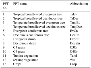
BETHY is a process-based terrestrial biosphere model at the core of the Carbon Cycle Data Assimilation System (CCDAS) (Rayner et al., 2005; Scholze et al., 2007). Full model description details can be found elsewhere (e.g. Rayner et al., 2005; Scholze et al., 2007; Knorr et al., 2010). Briefly, BETHY simulates carbon assimilation and plant and soil respiration within a full energy and water balance. The version used here also incorporates a leaf area dynamics module for prognostic leaf area index (LAI) as described in Knorr et al. (2010). This module includes parameters for leaf development, phenology, and senescence processes (hereby collectively termed leaf growth) to determine LAI in a scheme that incorporates temperature, water, and light limitations on growth and is capable of representing the major global phenology types (Knorr et al., 2010). This scheme also enables the representation of subgrid variability in leaf growth, representing the likely variability in growth triggers across a grid cell and the necessary mathematical form for differentiability between process parameters and state variables. The full BETHY model consists of four key modules: (i) energy and water balance; (ii) photosynthesis; (iii) leaf growth; and (iv) carbon balance. It represents variability in physiology and leaf growth of plant classes by 13 plant functional types (PFTs) (see Table 1) originally based on classifications by Wilson and Henderson-Sellers (1985). Each model grid cell may consist of up to three PFTs as defined by their grid cell fractional coverage.
SCOPE is a vertical (1-D) integrated radiative transfer and energy balance model with modules for photosynthesis and chlorophyll fluorescence (van der Tol et al., 2009). At present it is the only process-based model capable of simulating canopy-scale chlorophyll fluorescence. SCOPE incorporates the current understanding of chlorophyll fluorescence processes including canopy radiative transfer, reabsorption of fluorescence within the canopy, and the non-linear relationship between chlorophyll fluorescence quantum yield and other quenching processes (van der Tol et al., 2009, 2014). Leaf level chlorophyll fluorescence is coupled to the commonly used Farquhar and Collatz models for C3 and C4 photosynthesis, respectively (van der Tol et al., 2009). A current limitation of SCOPE is that there is no link between leaf level biochemistry and soil moisture. This is partly compensated for by changes in LAI due to soil moisture as simulated by BETHY.
The canopy radiative transfer and photosynthesis schemes of BETHY have been replaced by the corresponding schemes in SCOPE, including the components required for the calculation of chlorophyll fluorescence at leaf and canopy scales. The spatial resolution, vegetation (PFT) characteristics, leaf growth, and carbon balance are handled by BETHY. SCOPE therefore takes in climate forcing (meteorological and radiation data) and LAI from BETHY and returns GPP. BETHY calculates the canopy water balance, leaf growth, and net carbon fluxes, which will prove useful in future when assimilating other data streams (e.g. atmospheric CO2 concentration). Importantly, SCOPE provides a process-based link between SIF and GPP allowing the transfer of information from observations of SIF to simulated GPP. Subsequently, information from SIF may also be transferred to carbon fluxes resulting from GPP such as net ecosystem productivity.
2.2 Model process parameters
In this error propagation study, information from the SIF observations is used to constrain the uncertainty in the model process parameters. Parameters can either be global or differentiated by PFT. Global parameters apply to plants or soils everywhere, while PFT-dependent parameters enable differentiation between physiological and leaf growth traits. Some key parameters for this study such as the maximum carboxylation capacity (Vcmax) and chlorophyll a/b content (Cab) are considered PFT-dependent. From an ecophysiological perspective, there are other parameters specific to SCOPE that may be considered PFT-dependent such as the vegetation height and leaf angle distribution parameters. However, we have assumed them to be global to simplify the problem. GPP is relatively insensitive to these parameters, so this is not expected to impact the GPP uncertainty reduction results. Despite this, in a full assimilation with the SIF data, it may be necessary to make these PFT-dependent to improve the model-observed fit.
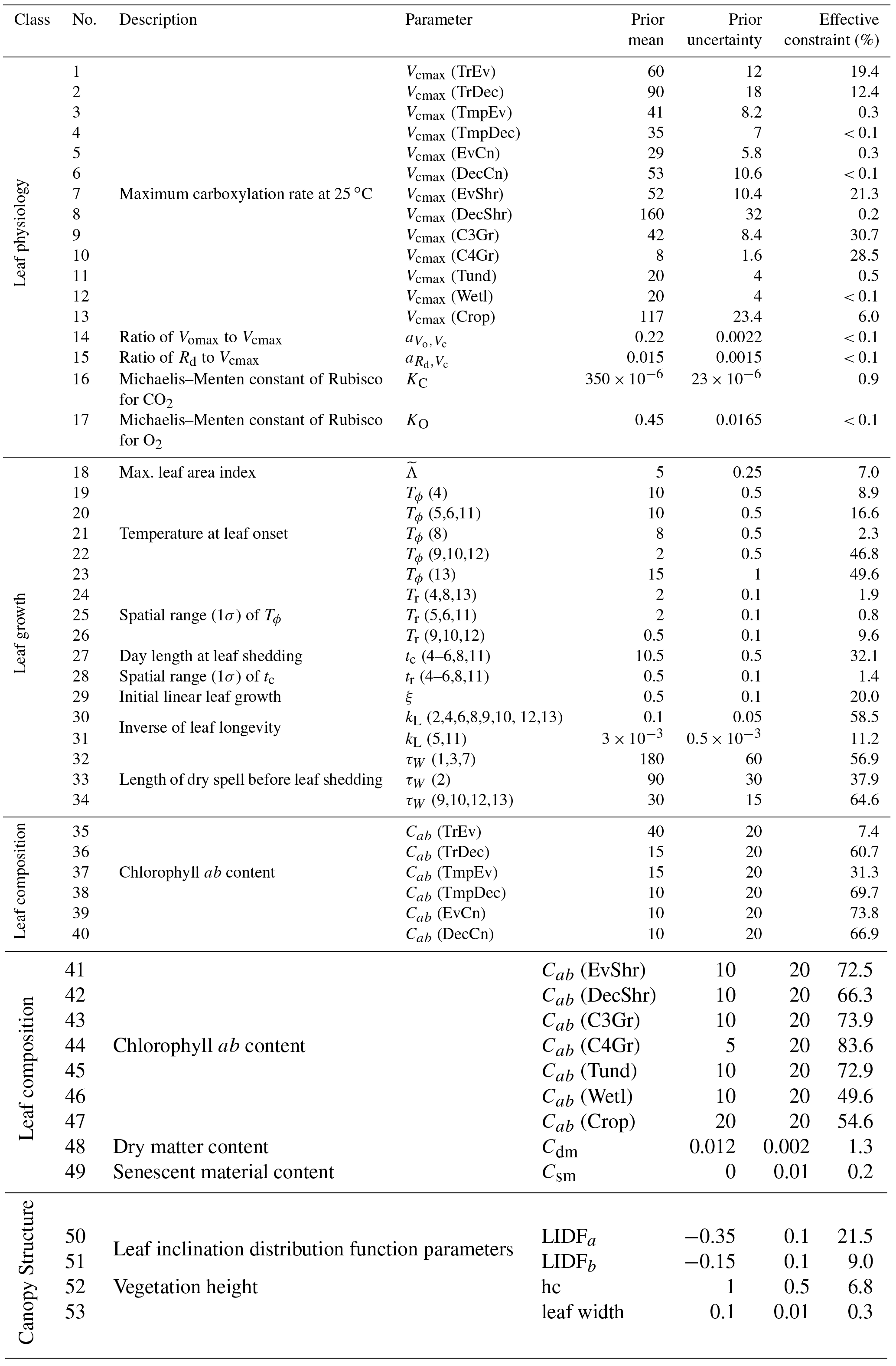
We expose 53 parameters from BETHY-SCOPE to the error propagation system (see Table A1). Each parameter is represented by a probability density function (PDF) which is assumed to be Gaussian. The mean and standard deviation for the prior parameters are shown in Table A1. The choice of the prior mean and uncertainty for parameters follows those used in previous studies (Kaminski et al., 2012; Knorr et al., 2010; Koffi et al., 2015). For new parameters that are not well characterized (e.g. SCOPE parameters), we assign relatively large prior uncertainties and mean values in line with the default SCOPE parameters and with Koffi et al. (2015). The choice of the prior may be considered important here, considering that we are using a linear approximation of the model around the prior and that the model is known to be non-linear. Therefore, sensitivities can differ depending upon the choice of the prior parameter values (Koffi et al., 2015).
There are 12 SCOPE parameters exposed, two of which are PFT-dependent (Cab and Vcmax). These parameters were chosen due to their importance in simulating SIF or GPP and due to sensitivity tests such as those performed by Verrelst et al. (2015). They include Cab, leaf dry matter content (Cdm), leaf senescent material fraction (Cs), two leaf distribution function parameters (LIDFa, LIDFb), vegetation height (hc), and leaf width. Leaf physiological parameters include Vcmax, Michaelis–Menten kinetic coefficients for CO2 (KC) and O2 (KO), the ratio of the Rubisco oxygenation rate to Vcmax (), and the ratio of day respiration to Vcmax ().
2.3 Uncertainty calculations
To calculate the uncertainty in parameter values following the constraint provided by the observational information of SIF (i.e. the posterior uncertainty), we propagate uncertainty from the observations onto the parameters. In order to perform this, we utilize a probabilistic framework where the state of information on parameters and observations is expressed by their corresponding PDFs (see Tarantola, 2005). The probability density of the errors in these quantities is assumed to be Gaussian; thus, they are describable by their mean and uncertainty. The prior information on parameters is quantified by a PDF in parameter space and the observational information by a PDF in observational space. The mean values for the parameters and observations are denoted by x and d, respectively. The uncertainty covariance matrices in parameter space and observational space are denoted by Cx and Cd, respectively.
For linear and weakly non-linear problems we can assume that Gaussian probability densities propagate forward through to Gaussian distributed simulated quantities (Tarantola, 2005). This permits linear error propagation from the input parameters to the model outputs. As mentioned earlier, estimating posterior uncertainties of the parameters for these types of problems can therefore be performed independently of the parameter estimation, in other words without the need to constrain the mean values of the parameters (Kaminski et al., 2010, 2012). This requires a matrix of partial derivatives of a target quantity with respect to its variables, also called a Jacobian matrix (H). This matrix represents the sensitivity of a simulated quantity (e.g. SIF, GPP) to the parameters. With the linear approximation, H is calculated around the prior parameter values (x0). This simplification of the model sensitivity brings limitations to the accuracy of the method. However, with the aggregation of subgrid variability across a model grid cell, sudden shifts in model sensitivity (e.g. step functions) are less likely or realistic; the present model accounts for these effects (Knorr et al., 2010). Additionally, because the parameter space can be very large, the use of prior knowledge on x0 helps to limit the effect of this problem as H at x0 likely provides a decent approximation of the true H that would occur at the global optimum (Tarantola, 2005). The simplification is also useful considering the high computational cost of calculating H.
To calculate the posterior parameter covariance matrix () following constraint by observational information, Cd, we use Eq. (1) (Tarantola, 2005).
where H expresses the Jacobian for SIF and HT the Jacobian transposed. Comparing parameter uncertainties in the prior () and the posterior () allows us to quantify the improvement in parameter precision following the observational constraint. The parameter uncertainties in and may be expressed as standard deviations (σ) by calculating the square root of their diagonal elements. We therefore assess the relative uncertainty reduction in parameters following SIF constraint, or “effective constraint”, with . This quantifies the effective constraint of the prior uncertainty and may be represented as a percentage decrease in σ uncertainty.
Formally, Cd represents the errors in the measurements and in the model-simulated counterpart (i.e. model error) (Scholze et al., 2016). As described further below in Sect. 2.4, we only consider the contribution of measurement errors to Cd in calculating posterior probabilities. However, to see if the assumptions that we have made about uncertainties are consistent with the model–data mismatch, we assess the reduced χ2 statistic () similar to a method employed by Kuppel et al. (2013). While more formal approaches to optimally estimate covariance parameters exist (Michalak et al., 2005), this metric can highlight whether we are neglecting a significant source of error in Cd, for example, model structural error. It also provides an indication of whether the model is capable of reproducing the measurements, given the assumed uncertainties. This is calculated by
where N is the number of degrees of freedom (equal to the number of observations in this case), M(x0) is the forward model-simulated SIF for the prior case, and d is the SIF observations. A greater than 1 would indicate that our assumptions around uncertainties may not be valid given the model–data mismatch and that the model cannot simulate the measurements (Michalak et al., 2005). Conversely, a of less than 1 indicates overconfidence in the assumed uncertainties. A value of approximately 1 is most desirable as it would indicate that our overall assumptions of uncertainties are valid. At the low resolution applied in the information content analysis, representation errors will be relatively large and may dominate other sources of error in Eq. (2) and therefore mask the actual ability of the model to simulate the measurements. For an assimilation of the data, the model would not be used at such a low resolution given the heterogeneity of the land surface and would instead be run at a higher spatial resolution. To help reduce the representation error, we utilize unpublished work that compares the forward model at a higher resolution (2∘ × 2∘) and with SIF observations from the OCO-2 (Orbiting Carbon Observatory-2) satellite for 2015. While this uses a slightly different parameterization, it is more credible and helps minimize the effects of representation error in determining whether the model can simulate the measurements. The error propagation analysis, however, benefits from using the low resolution as it greatly improves computational efficiency considering the computational demand of the model simulations and subsequent calculations.
The observational constraint introduces correlations into the posterior parameter distributions; thus, posterior parameter uncertainties are not wholly independent. Strong correlations in indicate parameters that cannot be resolved independently in an assimilation; however, their linear combinations can be. We calculate correlations in parameters by expressing the covariances as correlations as in Eq. (3) (see Tarantola, 2005, p. 71) by
where diagonal elements have a correlation equal to 1, while off-diagonals elements can range between −1 and 1. If large enough, these correlations can contribute significantly to the overall constraint of the target quantity (Bodman, 2013).
Using the parameter covariance matrix we can assess how parameter uncertainties propagate forward through the model onto uncertainty in GPP using the Jacobian rule of probabilities, the same method outlined in Rayner et al. (2005). This is the second stage of our error propagation study. Using we estimate the prior uncertainty in a vector of simulated target quantities (i.e. GPP). Similarly, using we estimate the posterior uncertainty in a vector of simulated target quantities. We calculate the uncertainty covariance of GPP (CGPP) using Eq. (4).
where HGPP is the Jacobian matrix of GPP with respect to the parameters. With this we can quantify the improvement in precision of simulated GPP by using either or in Eq. (4). Therefore, using the forward model, a statistical estimation scheme and a set of observational uncertainties, we can assess the information content of the SIF observations in the context of the model, its parameter set, and simulated GPP taking explicit consideration of uncertainties.
2.4 Uncertainty in observations and model forcing variables
The uncertainty in the measured data (hereafter, data) is a critical component in assessing the potential impact of an observing system on the estimation of carbon fluxes. Data uncertainties in SIF used here are calculated from the GOSAT satellite observations for 2010. These data are obtained from the ACOS (Atmospheric CO2 Observations from Space) project at a grid resolution of 3∘ × 3∘ (Frankenberg, 2018). As the model simulations are performed on a low-resolution grid (7.5∘ × 10∘), we aggregate these uncertainties to this resolution using Eq. (5) as described below in a way that conserves the information content from the original 3∘ × 3∘ observations.
We assume that the observations are independent and have uncorrelated errors, that is, they are distributed randomly. Assuming uncorrelated errors is, however, likely to overestimate the information content, particularly if using the standard error as the uncertainty. Although it has been used in recent studies with satellite SIF (e.g. Parazoo et al., 2014), the standard error under an assumption of uncorrelated errors is likely to be an overly optimistic approximation of the information content. For this study, we take a slightly conservative approach, scaling the calculated standard error by the square root of 2 as shown in Eq. (5). This effectively doubles the variance in an independent dimension and reduces the information content to compensate for the assumption of uncorrelated errors.
Through the aggregation of GOSAT grid cells to the model grid resolution, the number of independent measurements is reduced. To account for this and preserve the information content of the original GOSAT observations, the uncertainty in a given model grid cell is, approximately, divided by the square root of the number of GOSAT grid cells with SIF data that fall within that model grid cell (N). More precisely, we apply an area-weighting term in the equation (see Eq. A1 in the Appendix). This has the effect of scaling the uncertainty by the law but takes into account the fact that SIF is in physical units per unit area (i.e. W m−2 µm−1 sr−1) and that grid cells have different areas over different latitudes. A full description of this calculation and a detailed example is shown in the Appendix.
Therefore, the calculation of the SIF data uncertainties used here is approximated by Eq. (5) (for further details see Sect. A2 in the Appendix). For a given model grid cell, the variance (σ2) is approximately equal to the sum of the standard error of each individual GOSAT grid cell (σi) squared and then scaled by the number of individual GOSAT grid cells with data and the square root of 2.
The resulting annual observational uncertainties, shown in Fig. 3, appear to be much smaller than the uncertainties in individual GOSAT grid cells. In part this is due to the aggregation of multiple independent observations. Regions with more soundings across the year (e.g. the tropics) will also have smaller annual uncertainties.
Uncertainty in SIF observations may also have a systematic component. A known, potential systematic error in SIF stems from the zero-level offset calculated during the retrieval. Any error in the calculated zero-level offset will add to the measurement error. This radiometric correction is done to prevent biases in the SIF retrieval (Frankenberg et al., 2011a; Guanter et al., 2012), and this is performed monthly in the present GOSAT retrieval of SIF. In this case, it is systematic in the sense that it applies to multiple measurements. This type of error is distinguished from a bias, which is a systematic error with a precisely known magnitude and sign that should be corrected for. A bias cannot be incorporated into the present error propagation framework, whereas an error in the zero-level offset can be, provided it is Gaussian. To clarify, a retrieved measurement (d) of a quantity (e.g. SIF) at index point i can be given by
where is the true value at index point i, εi is a random variable with a variance of σ2 at index point i, and εz is a random variable that has some variance and is constant for a subset of the measurements (e.g. across a particular region or time). Based on previous analyses of the instruments, the error in zero-level offset in the SIF retrieval may be considered small (Frankenberg et al., 2011a, 2014). Here, we provide a more detailed assessment and characterization of the in-orbit systematic error. This is performed by assessing zero-level offset-corrected GOSAT SIF soundings over the non-fluorescent regions of Antarctica and central Greenland during January and July, respectively (see Fig. A2), in order to sample the error distribution of εz. These systematic errors appear quite small (±0.06 W m−2 µm−1 sr−1) and may vary seasonally due to factors such as atmospheric conditions or instrument-related causes (Guanter et al., 2012). We therefore assess the effect of a conservative systematic random error of size ±0.1 W m−2 µm−1 sr−1 in the zero-level offset seasonally. Practically, this means adding four (one for each season) extra uncertainty terms to Cx, corresponding to the estimated error, and adding four extra terms in H, which are scaling terms (equal to 1) applied to the corresponding season. Including these terms provides a sensitivity test to indicate how an error in the zero-level offset propagates through to uncertainty in GPP.
An additional source of uncertainty in model estimates of GPP is climate forcing. As mentioned by Koffi et al. (2015), while uncertainty in forcing such as incoming radiation is not considered in the current CCDAS set-up, it is considered to be an important variable in driving SIF (Verrelst et al., 2015) and GPP (Farquhar et al., 1980). Without a consideration of uncertainties in forcing variables, the uncertainty in GPP may be underestimated. Studies that use process-based models or empirically derived relationships do not explicitly consider such uncertainties (e.g. Beer et al., 2010). One such forcing variable is downward shortwave radiation (SWRad). Monthly means of SWRad are suggested to have a random error of 12 W m−2 (6 % of the mean) due mostly to uncertainty in clouds and aerosols (Kato et al., 2012). We therefore investigate how this random error in SWRad may be considered in GPP estimates. Furthermore, as SIF responds strongly to SWRad, there is the potential to utilize SIF observations as a constraint on the uncertainty in the forcing. We therefore conduct an additional experiment that incorporates the uncertainty in SWRad in the error propagation system. For this experiment an additional parameter representing SWRad is added to the inversion, which acts as a scaling factor for SWRad globally. We investigate the level of constraint SIF provides on this scaling factor and the subsequent effects of incorporating uncertainty in SWRad on uncertainty in GPP.
2.5 Model and data set-up
In this study BETHY-SCOPE is run for the year 2010 on the computationally efficient, low-resolution spatial grid (7.5∘ × 10∘). As the dynamical equations are the same for either low-resolution or high-resolution scales, the use of the low-resolution set-up is appropriate for an error propagation study as long as careful consideration is taken with observational uncertainties. Climate forcing in the form of daily meteorological input fields for running the model (precipitation, minimum and maximum temperatures, and incoming solar radiation) were obtained from the WATCH/ERA Interim data set (WFDEI; Weedon et al., 2014). Photosynthesis and fluorescence are simulated at an hourly time step but forced by the respective monthly mean diurnal cycle. Leaf growth and hydrology are simulated daily.
SIF is simulated at 755 nm, the wavelength corresponding to the GOSAT retrieval frequency and near the OCO-2 retrieval frequency (757 nm). We focus upon the constraint by SIF measurements at 13:00 local time as it closely corresponds to the local overpass time of the SIF-observing satellites GOSAT and OCO-2. However, we also investigate the effect of using alternative SIF-observing times (e.g. the GOME-2 satellite overpass time) and multiple observing times simultaneously on the constraint of GPP.
3.1 Prior mismatch
First, we present the results from Eq. (2) that determines whether the assumed uncertainties allow for coverage of observed SIF. As described in the methods, in this case we use a model forward run using the high-resolution version of the model and compare this with SIF observations from the OCO-2 satellite. We find that in this high-resolution case, close to the optimal value of 1.
3.2 Parameter uncertainties
As described in the “Methods” section, a key metric for assessing the relative uncertainty reduction, or effective constraint, is defined as . The effective constraint for all 53 parameters following constraint by SIF is shown in Fig. 1 and in Table A1. We define weak, moderate, and strong effective constraint as the relative uncertainty reduction from 1 to 10, 10 to 50, and > 50 %, respectively.
Parameters describing leaf composition (Cab, Cdm, Csm) generally achieve strong effective constraint from SIF. For 11 of the 13 Cab parameters the uncertainty is strongly constrained, between 50 and 84 %. SIF is highly sensitive to Cab, and we assign a relatively large prior uncertainty to these parameters, so considerable constraint is expected. For the tropical broadleaved evergreen tree PFT, however, the effective constraint on Cab is much lower at 7 %. For other leaf composition parameters Cdm and Csm, SIF effectively constrains the uncertainty by 1 and < 1 %, respectively.
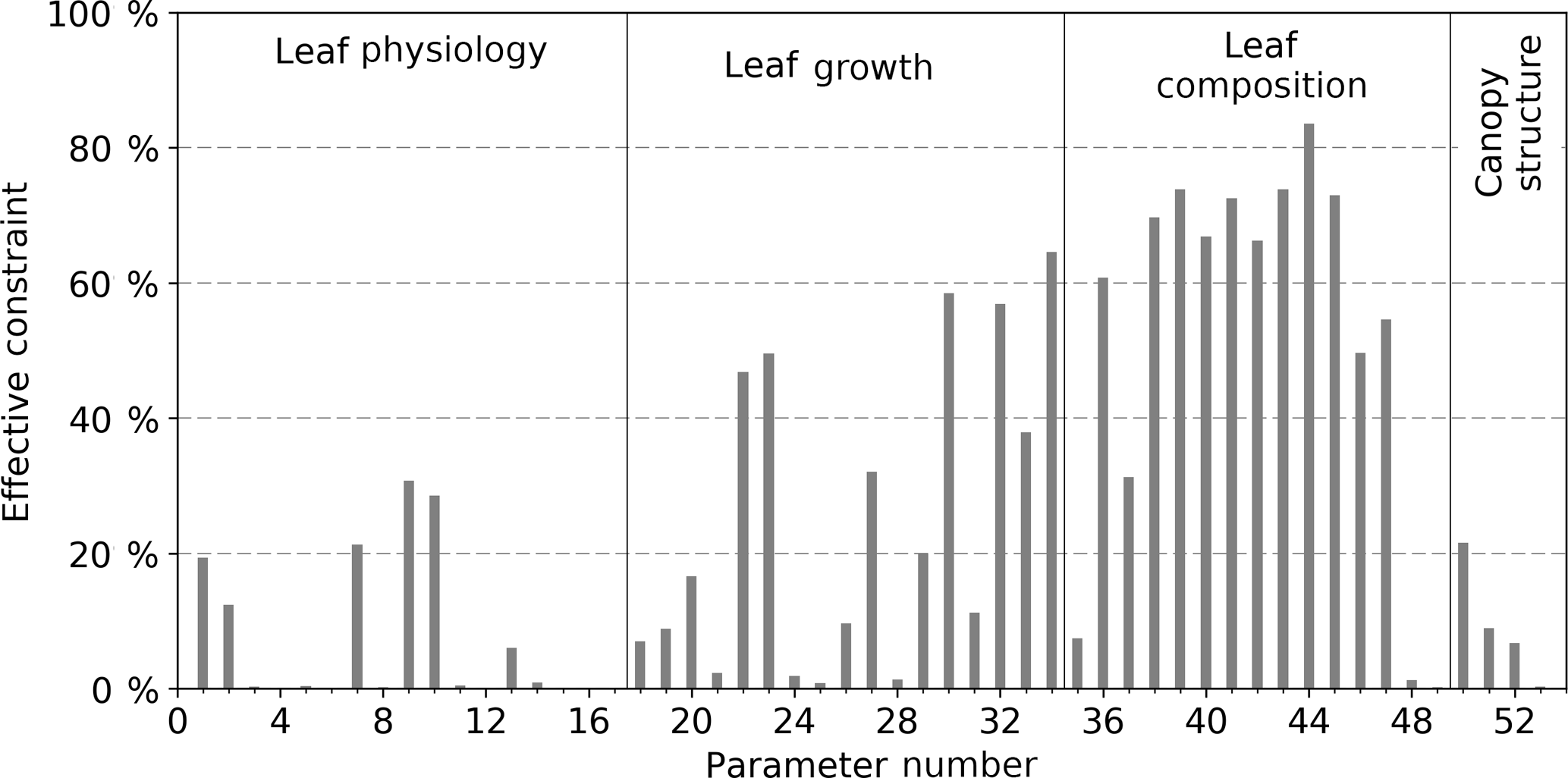
Figure 1Effective constraint of BETHY-SCOPE model process parameters from SIF observations. Only the parameter numbers are given; for the corresponding descriptions, see Table A1.
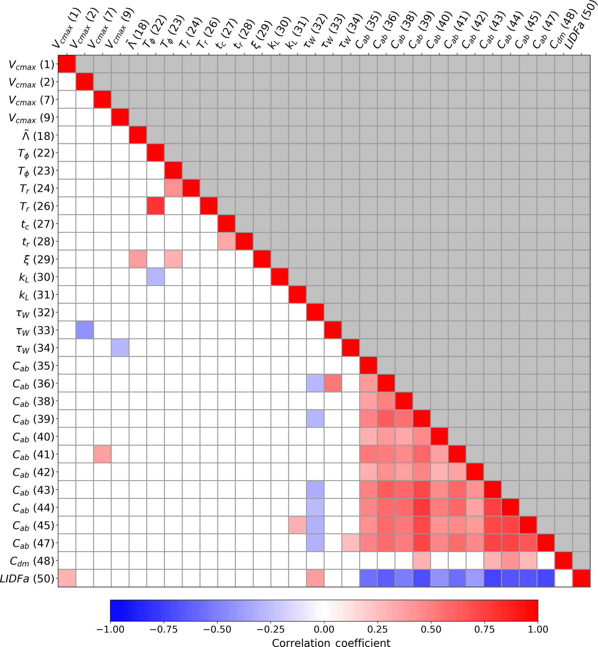
Figure 2Correlation coefficients (r value) between parameters in the posterior parameter covariance matrix (). This shows the magnitude and sign of correlations in posterior parameter uncertainties following constraint with SIF data. The axis labels show the parameter symbol and number as defined in Table A1. Only parameters with an absolute correlation coefficient > 0.25 with one or more other parameters are shown. Values above and below the diagonal are identical; therefore, those above are coloured grey.
Varied effective constraint is seen for the leaf growth parameters (parameters 18–34 in Table A1) that control phenology and leaf area. Four out of the seventeen leaf growth parameters exhibit strong uncertainty reductions. These parameters describe a variety of processes including the temperature at leaf onset, day length at leaf shedding, leaf longevity, and the expected length of dry spell before leaf shedding (τW) (see Table A1). The parameter τW is important in controlling leaf area, and it sees strong effective constraint from SIF, from 38 to 65 % depending upon which class of PFT it pertains to. For the parameters that are PFT-specific, there is generally a larger constraint seen when they relate to the C3Gr, C4Gr, and crops. For example, uncertainty in τW for grasses and crops is effectively constrained by 65 %.
Leaf physiological parameters (parameters 1–17 in Table A1) see a weak to moderate level of effective constraint. Of particular importance for simulating GPP is the PFT-specific parameter Vcmax. Effective constraint on Vcmax varies from < 1 up to 31 % depending upon the PFT of interest. Five PFTs that, combined, represent about 65 % of the land surface have their Vcmax parameters constrained by > 10 %. The global physiological parameters include the ratio of the maximum rate of oxygenation (Vomax) to Vcmax (), the ratio of dark respiration (Rd) to Vcmax (), and the Michaelis–Menten enzyme kinetic constants of Rubisco for CO2 (KC) and O2 (KO). These all see very weak effective constraint from SIF (< 1 %). Across all PFT-specific parameters, those that pertain to more dominant PFTs in terms of land surface coverage (e.g. C3 grass) tend to see stronger uncertainty reductions. This is largely due to them being exposed to more SIF observations.
Global canopy structure parameters (parameters 50–53 in Table A1) also see a weak to moderate constraint from SIF. In particular, the structural parameters LIDFa and LIDFb see their uncertainty reduced by 22 and 9 %, respectively. The parameters for vegetation height and leaf width, which are used to calculate the fluorescence “hot-spot” variable (see van der Tol et al., 2009), are effectively constrained by 7 and < 1 %, respectively.
With the observational constraint, correlations are introduced into the posterior parameter distributions. We assess these correlations using Eq. (3), shown in Fig. 2. We find strong (R≥0.5) positive correlations between nine of the PFT-specific Cab parameters. These are also negatively correlated with the leaf angle distribution parameter LIDFa. Thus, during a full assimilation with SIF data, only the sum of Cab and LIDFa can be resolved, not their individual values. Two leaf growth parameters are also strongly correlated: Tϕ with Tr. Smaller correlations are also present between the subset of parameters shown in Fig. 2.
To assess the effect of incorporating a systematic error from the observations into this analysis, we apply a seasonal σ error of 0.1 W m−2 µm−1 sr−1 (equivalent to εz in Eq. 6). This is incorporated as four additional parameters, one for each season, that scale the SIF signal across the globe. We find that the inclusion of this systematic error has a negligible effect on posterior uncertainties of the parameters. The difference in effective constraint between this sensitivity test case and the standard case above is < 1 % for any given parameter.
3.3 Uncertainty in GPP
To assess the constraint imposed by SIF on simulated GPP, we compare the prior and posterior uncertainty in GPP as calculated using Eq. (4). Similar to the assessment of parameter uncertainty reductions, to assess the effective constraint of SIF on GPP, we use a metric that measures the relative uncertainty reduction in σ from the prior to the posterior.
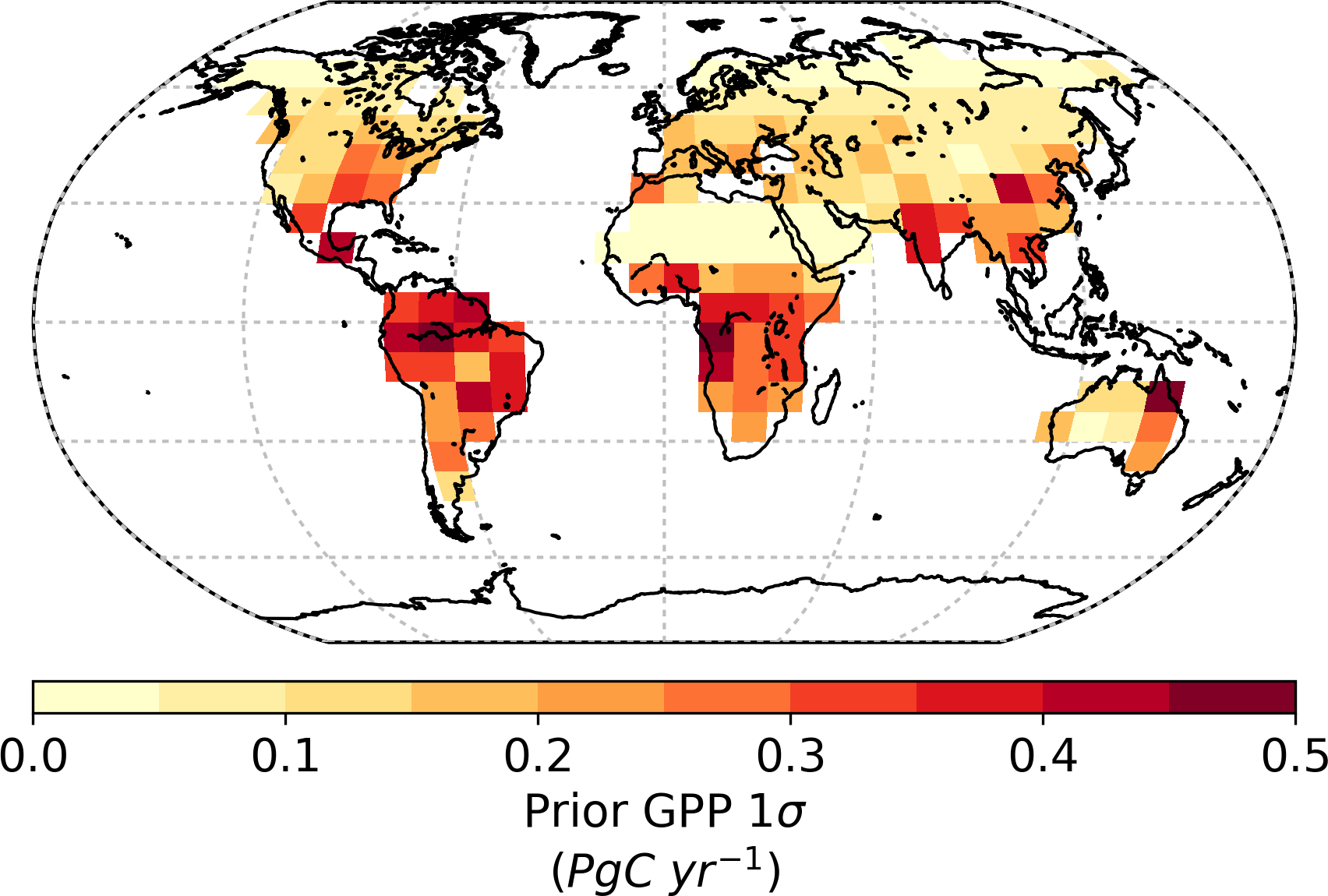
Global GPP from the prior model is approximately 164 Pg C yr−1 with a prior uncertainty (σ) of 19.0 Pg C yr−1. Utilizing SIF observations at 13:00 results in a 73 % reduction in the prior uncertainty, giving a posterior of 5.2 Pg C yr−1. Spatially, the prior uncertainty in GPP varies across the globe, with particularly large uncertainties in regions with high productivity (Fig. 4). This is to be expected, considering GPP uncertainty will typically correlate with GPP. In the posterior, it is clear that uncertainty in GPP is strongly reduced across the globe (Fig. 5). The relative uncertainty reduction (Fig. 6) appears to show smaller constraint of uncertainty in the boreal regions, likely due to the relatively large SIF uncertainty (Fig. 3) and low prior uncertainty in GPP (Fig. 4).
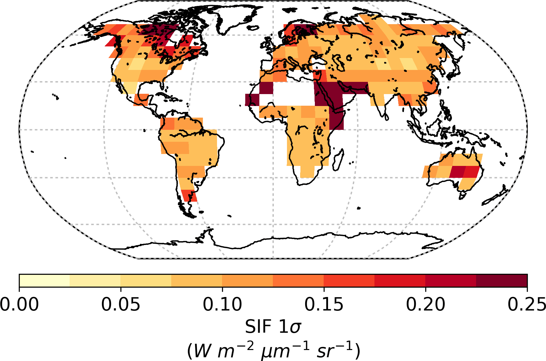
Figure 3Annual observational uncertainty in SIF interpolated from GOSAT observations for 2010.
To assess which parameters contribute to the uncertainty in GPP for the prior and posterior, we can conduct a linear analysis of the uncertainty contributions. Typically this technique can only be used for the prior as the correlations in posterior parameter uncertainties, excluded from the linear analysis, also contribute toward the overall constraint. However, we can assess the contribution of these correlations to the constraint of GPP by setting the off-diagonal elements in to zero and using it in Eq. (4); the difference between this and the standard case that uses the full equates to the contribution of correlations. We find that the contribution of these correlations to the constraint of GPP is small (0.16 Pg C yr−1 or < 1 %); thus, we can assume that the linear analysis technique holds for the posterior as well. This finding is supported by the correlation analysis in posterior parameter uncertainties which showed few significant correlations in parameters relevant for GPP. This result is encouraging as it indicates that the parameters in a SIF assimilation system contributing most to the constraint of GPP are capable of being resolved independently.

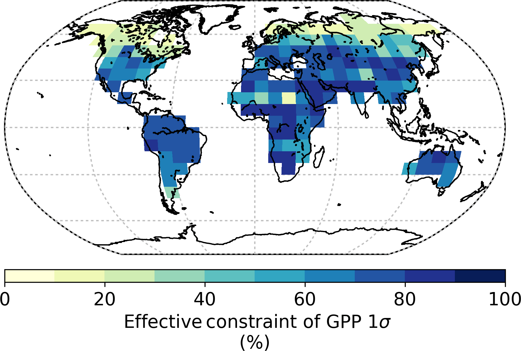
Figure 6Relative uncertainty reduction (i.e. effective constraint) of parametric uncertainty in annual GPP from prior to posterior.
Using a linear analysis of the uncertainty, we find that uncertainty in global annual GPP in the prior and posterior stems from different processes. For the prior we find that the uncertainty in GPP is dominated, at 89 %, by parameters describing leaf growth processes. Of these, a single parameter, τW, for C3 grass, C4 grass, and crops makes up 74 % of the uncertainty in global annual GPP. Parameters representing physiological processes account for about 9 % of prior uncertainty, most of which stems from the Vcmax parameters. Parameters for Cab only account for 2.5 % of the prior uncertainty.
For the posterior, which has a lower overall uncertainty in GPP, uncertainty is dominated by parameters representing physiological processes. Physiological parameters account for 67 % of the uncertainty in posterior annual GPP, with Vcmax parameters accounting for 32 % and the Michaelis–Menten constant of Rubisco for CO2 (KC) accounting for 30 %. The relative contribution by leaf growth parameters is reduced to 33 %, and for , it is 15 %. For Cab the relative contribution is smaller than the prior at < 1 %. This shift in which parameters contribute to the relative uncertainty in GPP between the prior and the posterior demonstrates how effectively SIF constrains leaf growth processes. Uncertainties in physiological parameters are constrained less than the leaf growth parameters, which results in them contributing more in relative terms to the posterior uncertainty in GPP.
Regionally, we split the land into three regions, the Boreal region (above 45∘ N), the Temperate North (30 to 45∘ N), and the Tropics (30∘ S to 30∘ N). SIF constraint on annual GPP varies substantially across different regions of the globe, with a relative uncertainty reduction in of 48, 82, and 79 % for the Boreal, Temperate North, and Tropics regions, respectively. In Fig. 7 we show the contribution of parameter classes (leaf physiology, leaf growth, leaf composition, and canopy structure; see Table A1 for details) to the parametric uncertainty in GPP across the year for each of these regions. From Fig. 7 it can be seen that the Boreal and Temperate North regions exhibit seasonal differences in GPP uncertainty, mostly due to the seasonal cycle in GPP, and in the constraint SIF provides. This is caused by seasonal dependencies in the sensitivity of SIF and GPP to certain processes (e.g. leaf development versus leaf senescence) as well as seasonal differences in the density of observations in these regions. There are far fewer GOSAT satellite observations during Boreal autumn and winter; thus, there are fewer observations to constrain processes controlling GPP during this time.
During the start of the growing season leaf physiology, in particular photosynthetic rate constants (Vcmax), plays a larger role in GPP uncertainty, whereas later in the growing season during the warmest months leaf growth, via water limitation on leaf area of grasses, plays a larger role. Therefore in the Boreal region, where the strongest seasonality in constraint is seen, from July through to January SIF constrains GPP by > 60 %. Uncertainty in GPP during these months is dominated by the leaf growth parameters and kL along with Cab (for EvCn), all of which receive considerable constraint from SIF. From February to June however, SIF constrains GPP by less than 50 %, as a large proportion of the uncertainty arises from the less constrained Vcmax parameters. Following SIF constraint, uncertainty in Boreal GPP stems mostly from uncertainty in leaf physiology, particularly for the EvCn PFT. Similar differences between seasonal constraint are seen for the Temperate North, although with a smaller seasonal variation in SIF constraint that ranges between 74 and 87 % across the year.
For the Tropics uncertainty reduction in GPP is about 80 % across the year. Uncertainty in the prior is dominated by the leaf growth parameters and in particular the τW parameters controlling water-limited leaf area. SIF constraint is primarily propagated through the τW parameters to GPP resulting in a well-constrained posterior with a σ uncertainty of 1.6 Pg C yr−1 in the annual GPP of the Tropics. Although moderate constraint is seen in the key PFT-specific parameter Vcmax for the dominant tropical PFTs (see Fig. 1), in the posterior these parameters contribute to roughly 35 % of the uncertainty in annual GPP.

Figure 7Contribution of parameter classes to parametric uncertainty in monthly GPP for three regions (see Table A1 for details on these parameter classes). For each month, the bar on the left is the prior and the bar on the right is the posterior. Uncertainties are represented as variances; thus, the units are in Pg C yr−1 squared, and, for clarity, the y axes are on a quadratic-transformed scale.
3.4 Diurnal SIF constraint
With this set-up it is possible to test how the SIF constraint on GPP might change with alternative observational times. Considering this, we test how the constraint on GPP changes when assimilating observations of SIF from alternative times of the day, assuming the same number of observations and the same observational uncertainty as used above. From this we see that different observing times yield differences in the posterior uncertainty and the effective constraint of GPP (see Fig. 8). The constraint on global annual GPP when using SIF-observing times between 09:00 and 15:00 is quite similar, with the posterior uncertainty in global annual GPP ranging from 5.0 Pg C yr−1 (effective constraint of 74 %) to 6.0 Pg C yr−1 (effective constraint of 68 %). The most significant constraint on GPP is obtained when using SIF observations at between 11:00 and 13:00, nearest to the peak in the diurnal cycle of both GPP and SIF.
We also test the effect of utilizing SIF measurements at multiple times of the day simultaneously. We select the times 08:00, 12 noon, and 16:00, replicating a theoretical geostationary satellite. For this experiment we first test the effect of increasing the number of observations by a factor of 3, assuming the same uncertainty for the three observation times. Second, we also increase the number of observations by a factor of 3, but scale the variance of these observations by one third. Using this second test we can assess whether differences in parameter sensitivities of SIF and GPP at the different times of the day add value in the overall constraint.
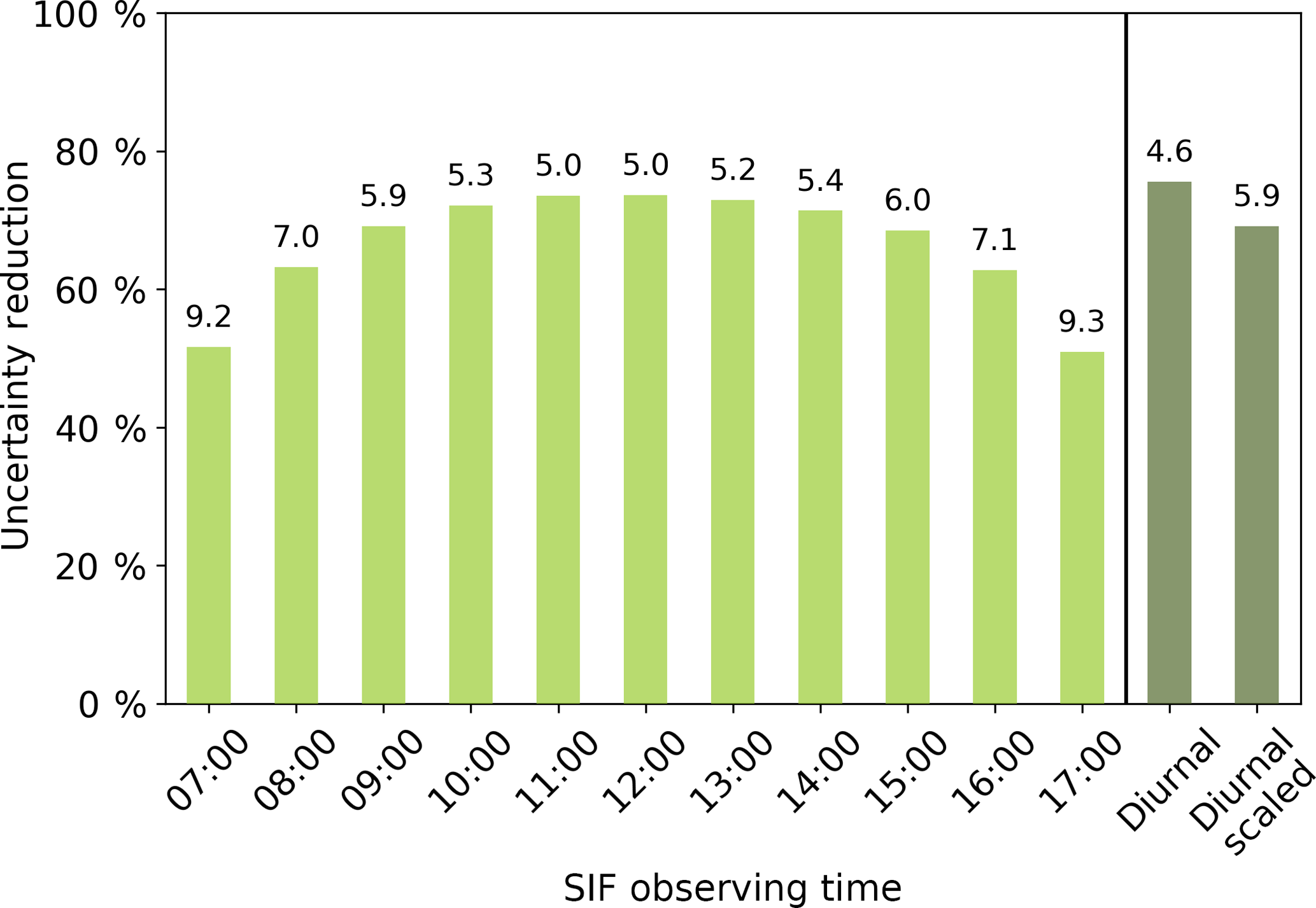
Figure 8Effective constraint on global annual GPP for different observing times and the two diurnal cycle configurations. Values at the top of the bars correspond to the posterior uncertainty (σ) in global annual GPP.
Using a diurnal cycle of observations results in a posterior uncertainty of 4.6 Pg C yr−1 or an effective constraint of 76 % as in Fig. 8. This is an extra 2 % constraint on the uncertainty in GPP compared with observations at 12:00 noon alone. If we use a diurnal cycle of observations with scaled uncertainties, we see a slightly reduced constraint on GPP where the posterior uncertainty is 5.9 Pg C yr−1, equivalent to an effective constraint of 69 % (Fig. 8).
3.5 Incorporating uncertainty in radiation
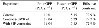
In order to assess the effects of incorporating uncertainty in SWRad, we conduct three experiments. First is a control run, equivalent to using SIF at 13:00 as before. The second includes uncertainty in SWRad by adding it into the posterior uncertainty calculation; this might be done normally when accounting for uncertainty in forcing. The third experiment incorporates uncertainty in SWRad into the error propagation system with SIF, such that the uncertainty in SWRad may be constrained. This third experiment effectively treats SWRad as a model parameter by adding an extra row and column to Cx.
Including the uncertainty in SWRad in the calculation of posterior uncertainty in GPP results in an additional 0.03 Pg C yr−1 to the prior uncertainty in global annual GPP. This is a small effect relative to the parametric uncertainties. Moreover, if we incorporate SWRad uncertainty into the error propagation system, we see that this additional uncertainty is mitigated by the SIF constraint. With SWRad uncertainty included, the posterior uncertainty in GPP remains at 5.15 Pg C yr−1, equivalent to the case without accounting for uncertainty in SWRad, in both cases resulting in a relative reduction in the GPP uncertainty by 72.9 %. This mitigation of the additional uncertainty from SWRad is possible because both SIF and GPP are strongly sensitive to it; thus, any constraint on SWRad from SIF is also propagated through to GPP.
Table 2Parametric uncertainty and effective constraint of global annual GPP for each of the SWDown experiments. Prior and posterior values shown are the 1 standard deviation (σ) uncertainty in global annual GPP.
By assessing the prior and posterior uncertainty in SWRad in and , respectively, we can assess the effective constraint following the use of SIF in the error propagation system. We find that SIF constrains the SWRad uncertainty by about 29 %. This gain in information on SWRad naturally results in less information being available for other parameters. The relative uncertainty reduction for most parameters decreases by a few percent. For example most Cab parameters see a decrease in effective constraint of around 1 % and Vcmax parameters up to 3 %. With GPP exhibiting low sensitivity to Cab parameters and strong sensitivity to SWRad, the transfer of information from Cab to SWRad results in an overall mitigated effect of SWRad uncertainty on GPP.
The results presented show that with 1 year of satellite SIF data observed at the GOSAT and OCO-2 satellite overpass time and SIF retrieval wavelength, we can constrain a large portion of the BETHY-SCOPE parameter space and ultimately yield a parametric uncertainty in global annual GPP of ±5.2 Pg C yr−1. The parametric uncertainty in the prior is approximately 12 % of the global annual GPP. Following the addition of SIF information, this is reduced to about 3 % of global annual GPP. This constitutes a reduction in parametric uncertainty of 73 % relative to the prior. Although this data-driven constraint is model dependent, it is an improvement on the often reported uncertainty of ±8 Pg C yr−1 from the empirical-model-based upscaled product of Beer et al. (2010).
We note that this analysis is likely to underestimate the constraint that SIF could provide on GPP as it is performed with uncertainties calculated from the GOSAT SIF 3∘ × 3∘ spatial-resolution observations. With the use of higher-resolution observations such as those from OCO-2, the constraint will get stronger. Similarly, with a longer time series of data, there will be stronger constraint. This occurs because the number of independent observations increases while the number of parameters remain constant.
This error propagation analysis does not assess how model SIF compares with observed SIF. However, our finding that the is near the optimal value of 1 provides evidence that the range of possible model SIF realizations, given our assumptions of parameter and data uncertainties, can provide coverage of the observed SIF. While this is not evidence that each specific uncertainty (e.g. parameters, model, measurement) is optimal (Michalak et al., 2005), it does suggest that overall the assumptions are valid and that we are not overconfident in or underestimating covariances. We reiterate that the test is performed using a higher spatial-resolution model and measured data because this is the resolution that would be applied in an assimilation of the data and this reduces the effects of representation errors. The error propagation analysis, however, benefits from using a low resolution as it greatly improves computational efficiency considering the simulations, and calculations are computationally demanding.
We also find that the effect of incorporating the error in the zero-level offset correction in the SIF observations is negligible on posterior parametric uncertainties. This may be negligible because, for a given season, this systematic uncertainty applies across all data points; thus, it scales all of the SIF values and therefore the sensitivities as well. In any case, the systematic error in the zero-level offset-corrected data assessed here (Fig. A2) appears small.
The constraint on global GPP is similar when assimilating SIF at any time between 09:00 and 15:00. Assimilating observations at the daily maximum of SIF and GPP provides the strongest constraint as both quantities exhibit the strongest parameter sensitivities at these times. Depending upon the state of the vegetation and the environmental stress conditions, maximum SIF and GPP may occur anywhere between mid-morning and early afternoon. Therefore, we expect that the effective use of different satellite-retrieved SIF observations for assimilation studies will depend not so much on their observing time but more on the spatiotemporal resolution, measurement precision, and subsequent uncertainty.
A confounding factor in this expectation is the uncertain role of physiological stress on the diurnal cycle of SIF and GPP and on modelling capabilities of these processes. Multiple studies have shown that various forms of environmental stress result in the downregulation of PSII and changes in the fluorescence yield, particularly evident across the diurnal cycle (Carter et al., 2004; Daumard et al., 2010; Flexas et al., 1999, 2000, 2002; Freedman et al., 2002). By incorporating SIF observations at multiple times of the day, we hypothesized that there could be improvements in the overall constraint on GPP as the SIF observations would capture the vegetation in different states of stress. We saw only minor improvements in the constraint and less constraint if we assumed no additional information in the observations (i.e. with scaled uncertainty). Thus, the difference in model parameter sensitivities of SIF and GPP at other times across the diurnal cycle was not sufficient to add value to the constraint. Additionally, the constraint is worse with these scaled observational uncertainties as we are effectively removing some useful observational information at midday, the time that provides the highest sensitivities, and getting extra observational information at the lower-sensitivity times of 08:00 and 16:00. This may be due to limitations of the model. Although BETHY-SCOPE simulates light-induced downregulation of PSII, there is no mechanism present to simulate other forms of stress that might be expected to emerge across the diurnal cycle. However, even with a perfect model, the spatial footprint and spatiotemporal averaging of satellite observations may smooth over stress signals. Considering these confounding factors, incorporating individual SIF soundings could help remedy this problem, and there is no technical reason other than the high computational requirements that would prevent a data assimilation system from doing so.
The constraint of SIF on GPP occurs via multiple processes including leaf growth, leaf composition, physiology, and canopy structure. For the prior, uncertainty in global GPP is dominated by leaf growth processes. There is a clear and direct link between leaf growth processes and GPP (Baldocchi, 2008) as the dynamics of leaf area influences canopy absorbed photosynthetically active radiation (APAR), which in turn strongly influences GPP. Leaf growth parameter uncertainties are relatively large in the prior, with coefficients of variation up to 50 %. It is perhaps no surprise then that these parameters project a large uncertainty onto GPP. Regardless, both GPP and SIF respond similarly to the leaf growth parameters, so information from observations of SIF can provide a direct constraint on GPP in this way. Many leaf growth parameters, particularly for grasses, crops, and deciduous trees and shrubs, receive a constraint of > 40 % from SIF; thus, the overall contribution of leaf growth parameters in the posterior is considerably reduced.
Of particular importance is the parameter describing water limitation on leaf growth (τW), which accounts for about 80 % of the prior uncertainty in global GPP. Model SIF and GPP are highly sensitive to this parameter; hence, there are large values in H and HGPP pertaining to τW. This relates to the model formulation as many of the leaf growth parameters determine phenological processes such as temperature or light-dependent growth triggers (i.e. temporal evolution of leaf area), while τW is the only process parameter controlling leaf area other than intrinsic maximum LAI () (Knorr et al., 2010). Additionally, as we assume little prior knowledge for τW (i.e. it is highly uncertain) it projects a relatively large uncertainty onto GPP.
At the global scale, τW for crops, C3 grasses, and C4 grasses is particularly important. Combined, these three PFTs cover about 47 % of the land surface and account for just over 50 % of global annual GPP in the present model set-up. Although this contribution to global GPP may seem high, it is based on the prior estimate. In a recent study by Scholze et al. (2016), where atmospheric CO2 concentration and SMOS (Soil Moisture and Ocean Salinity) soil moisture were assimilated into BETHY, the posterior value for shifted approximately 3 standard deviations away from the prior, the result of which would have been a large change in the GPP of these PFTs. This exposes a limitation of the present study as we can predict and quantify how SIF will constrain the uncertainty in process parameters and GPP, but we cannot predict how their values will change.
The constraint SIF provides on leaf growth processes is also perhaps achievable from other remote-sensing products such as FAPAR (e.g. Kaminski et al., 2012). A direct comparative study would be required to assess the advantages and disadvantages of each observational constraint. Nevertheless, issues arise with these alternative observations when observing dense canopies (Yang et al., 2015) or vegetation with high photosynthetic rates such as crops (Guanter et al., 2014). Information on maximum potential LAI () and parameters pertaining to understorey shrubs and grasses are therefore also limited (Knorr et al., 2010). A strong benefit of SIF is that it shows minimal saturation effects (e.g. Yang et al., 2015), especially beyond 700 nm, where most current satellite SIF measurements are made.
The strong constraint SIF provides on leaf growth processes indicates that it is likely to provide improved monitoring of key phenological processes such as the timing of leaf onset, leaf senescence, and growing season length as also suggested by Joiner et al. (2014). This will be highly useful in interpreting results from a full assimilation with SIF as the posterior process parameter values can be compared with independent ecophysiological data, taking spatial scale issues into consideration.
Beyond observing LAI dynamics SIF can also provide critical insights into physiological processes (e.g. Walther et al., 2016). We see here that SIF provides a weak to moderate constraint on a range of physiological parameters, including up to 30 % constraint on Vcmax parameters. The limited constraint on these parameters results in the posterior being dominated by uncertainty in the parameters representing physiological processes. This is in line with Koffi et al. (2015), who found limited sensitivity of simulated SIF to Vcmax. We note that under certain conditions, where other key variables are well known, SIF can be used to retrieve Vcmax (Zhang et al., 2014). The ability of SIF to provide information on physiological processes at all will provide researchers with a powerful new insight into the spatiotemporal patterns of GPP. As was shown by Walther et al. (2016) and Yang et al. (2015), this is particularly important for evergreen vegetation as changes in photosynthetic activity are not always reflected by changes in traditional vegetation indices.
Chlorophyll content here constitutes a classic nuisance variable. A nuisance variable is one that is not perfectly known and impacts the observations we wish to use but not the target variable (Rayner et al., 2005). However, exploiting the well-documented correlation between leaf nitrogen content, Vcmax, and Cab may help curtail this problem (Evans, 1989; Kattge et al., 2009). Houborg et al. (2013) demonstrated that by including a semi-mechanistic relationship between these variables in the Community Land Model and using satellite-based estimates of chlorophyll to derive Vcmax, there is significant improvement in predictions of carbon fluxes over a field site. Implementing such a semi-mechanistic link in a data assimilation system would enable the strong constraint that SIF provides on Cab to feed more directly into GPP. However, in this study it is assumed Cab and Vcmax can be resolved independently, which may not be the case considering that ecophysiological studies have shown that the two parameters are commonly correlated.
Almost all terrestrial carbon cycle models use down-welling radiation at the Earth's surface as an input variable. Any uncertainty in this forcing will translate into uncertainty in carbon fluxes including GPP, and few studies consider such uncertainties. A known systematic error (i.e. bias) in forcing variables (e.g. Boilley and Wald, 2015) cannot be considered in the present error propagation system; however, in such a case a correction to the data should be performed as it will bias carbon flux estimates. For random errors that cannot be removed, however, they may be considered in the uncertainty in carbon flux estimates using error propagation. At the global scale, Kato et al. (2012) used a perturbation study, along with modelled irradiance and remotely sensed measurements to compute a random error (σ) of 12 W m−2 for monthly gridded downward shortwave radiation over the land. We considered this uncertainty by incorporating it into the error propagation system with SIF. While including this forcing uncertainty in the prior increases the prior uncertainty in GPP, incorporating the former into the error propagation analysis with the SIF observations mitigates the downstream effect on GPP. SIF can therefore provide useful information on the SWRad forcing via a data assimilation system. The consideration of uncertainties in forcing variables such as SWRad on terrestrial carbon fluxes is important when estimating the uncertainty in GPP. However, the effect on uncertainty in GPP may be strongly reduced by using SIF observations.
The results presented here demonstrate how SIF observations may be utilized to optimize a process-based terrestrial biosphere model and constrain uncertainty in simulated GPP. These results are, however, model dependent. The assumption is that the model simulates the most important processes driving SIF and GPP. Some key, remaining unknowns include how processes such as environmental stress, three-dimensional canopy structure effects, or nitrogen cycling may affect the SIF signal. As better understanding is developed of the role that these processes play, modelling capabilities will also be improved. Additionally, a different set of prior parameter values will alter the results due to changes in H. The use of prior knowledge, based on ecophysiological data and its probable range, is critical to curtailing this problem. The choice of how to spatially differentiate the parameters will also affect results (Ziehn et al., 2011). Selecting an optimal parameter set that has the fewest degrees of freedom yet provides the best fit to the observational data is outside the scope of this study, however. The implementation of a parameter estimation scheme in a full data assimilation system with SIF and other observational data will help address these challenges. Earlier work by Koffi et al. (2015) demonstrated that the model can simulate the patterns of observed satellite SIF quite well, indicating that the model can incorporate the data. Further work will be needed to assess how well the model can simulate patterns of SIF with an optimized, realistic parameter set.
We assessed the ability of satellite SIF observations to constrain uncertainty in model parameters and uncertainty in spatiotemporal patterns of simulated GPP using a process-based terrestrial biosphere model. The results show that there is a strong constraint of parametric uncertainties across a wide range of processes including leaf growth dynamics and leaf physiology when assimilating just 1 year of SIF observations. Combined, the SIF constraint on parametric uncertainties propagates through to a strong reduction in uncertainty in GPP. The prior uncertainty in global annual GPP is reduced by 73 % from 19.0 to 5.2 Pg C yr−1. Although model dependent, this result demonstrates the potential of SIF observations to improve our understanding of GPP. We also showed that a data assimilation framework with error propagation such as this allows us to account for uncertainty in model forcing such as SWRad. Surprisingly, by including it into this framework with SIF observations, there is a net-zero effect on uncertainty in GPP due to the sensitivity of both SIF and GPP to radiation. This study is a crucial first step toward assimilating satellite SIF data to estimate spatiotemporal patterns of GPP. With the addition of other observational constraints such as atmospheric CO2 concentration or soil moisture there is also the possibility of accurately disaggregating the net carbon flux into its component fluxes – GPP and ecosystem respiration. Indeed, with these additional, complementary observations of the terrestrial biosphere further constraint could be gained as other regions of parameter space can be resolved (Scholze et al., 2016).
The BETHY-SCOPE model code is available upon request from the authors. The GOSAT satellite SIF data used in this paper are from the ACOS project (version B3.5) (Frankenberg, 2018).
A1 Model process parameters
Table A1BETHY-SCOPE process parameters along with their prior and optimized uncertainties following SIF constraint, represented as 1 standard deviation. Relative uncertainty reduction (i.e. effective constraint) is reported for the error propagation with low-resolution and high-resolution SIF observations. Units are as follows: Vcmax – µmol(CO2) ; , and – dimensionless ratios; KC and KO – bar; – m2 m−2; Tϕ – ∘C; Tr – ∘C; tc – hours; tr – hours; ξ – d−1; kL – d−1; τW – days; Cab – µg cm−2; Cdm – g cm−2; Csm – dimensionless fraction; hc – m; leaf width – m.
A2 GOSAT SIF uncertainty calculations
To obtain the variance of a target grid cell at the model grid resolution (ylat, xlon), we first determine the area-weighted variance of each GOSAT grid cell (ilat, jlon) within that target grid cell. The area weighting per GOSAT grid cell () is calculated as the area divided by the total area of the target grid cell. This enables us to account for different
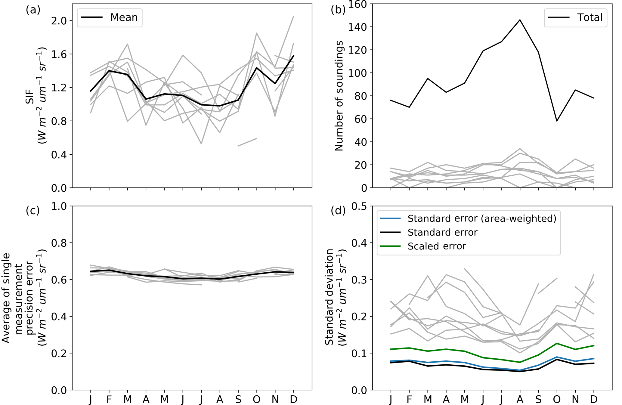
Figure A1An example of the GOSAT SIF data and uncertainty calculations over a low-resolution model grid cell centred over the Amazon forest at 3.75∘ S and 65∘ W. Grey lines show individual 3∘ × 3∘ GOSAT grid cells. Black lines show the aggregated data for the 7.5∘ × 10∘ model grid cell. Panel (d) shows the calculated uncertainty (standard deviation) at the model grid resolution in black, blue, and green. The black line is the standard error calculated using Eq. (5); the blue line is the standard error calculated using Eq. (A1); the green line is the same as the blue but scaled by to account for correlated errors which are used in this study.
grid cell sizes considering that SIF is in physical units per unit area. We then sum the area-weighted variances and scale this uncertainty by the square root of 2 (see Eq. 5). Scaling the uncertainty in this way effectively doubles the variance in an independent dimension.
A3 Systematic error in GOSAT SIF observations
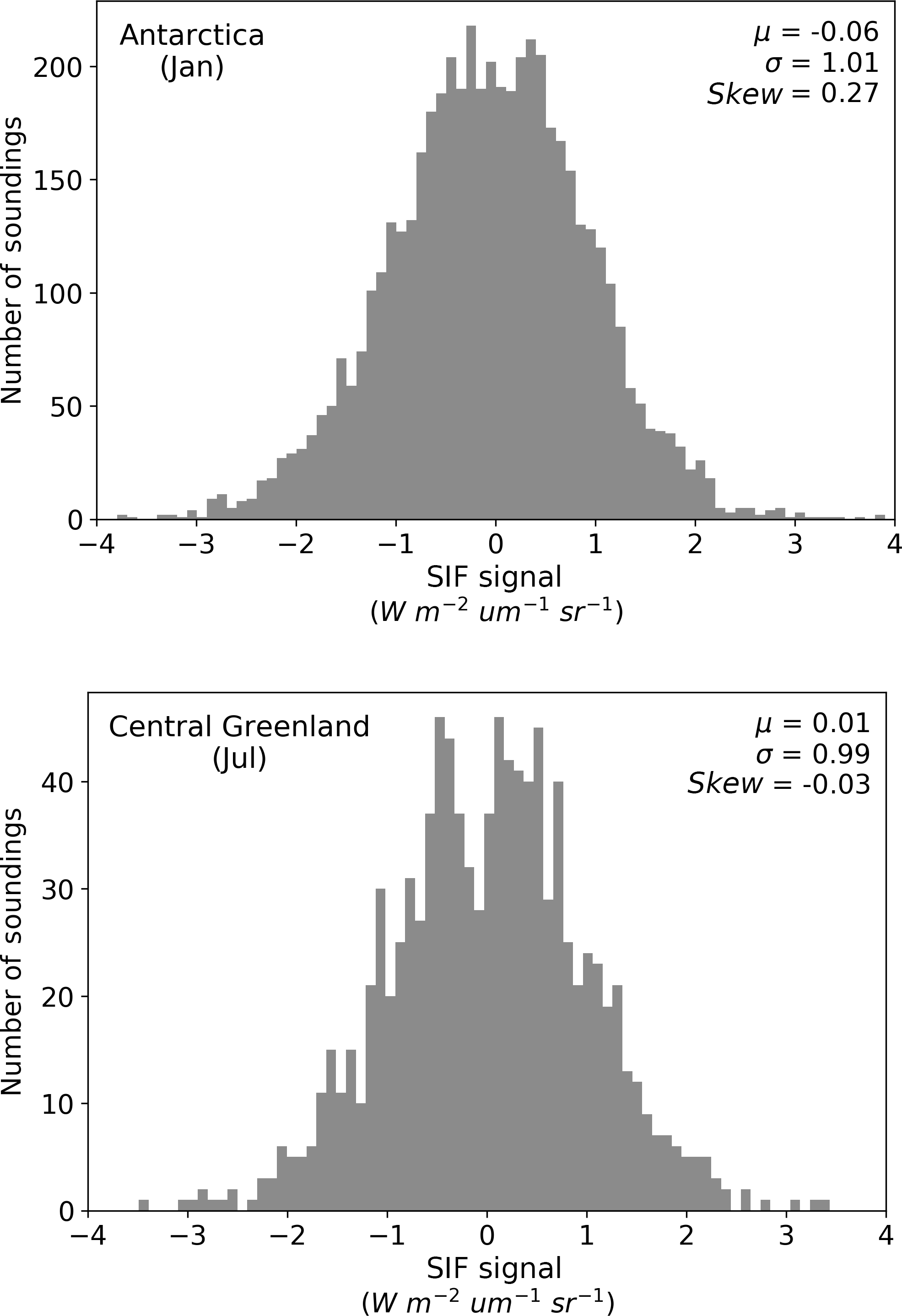
Figure A2Analysis of systematic errors in the GOSAT SIF observations. We assess the zero-level offset-corrected GOSAT SIF soundings over two ice-covered and therefore non-fluorescent regions. The first is Antarctica in January, between latitudes 70 and 80∘ S and longitudes 75∘ W to 155∘ E. The second is central Greenland in July, between latitudes 73 to 80∘ N and longitudes 30 to 52∘ W. With no systematic error, the mean (μ) value of the distribution should be on 0. As is shown, μ is non-zero and varies in sign and magnitude between January and July. This test samples the error distribution in the zero-level offset (i.e. εz in Eq. 6).
The authors declare that they have no conflict of interest.
Alexander Norton was partly supported by an Australian Postgraduate Award
provided by the Australian Government and a CSIRO OCE Scholarship. The
research was funded, in part, by the ARC Centre of Excellence for Climate
System Science (grant CE110001028).
Edited by:
Tomomichi Kato
Reviewed by: Sylvain Kuppel and one anonymous
referee
Baker, N. R.: Chlorophyll fluorescence: a probe of photosynthesis in vivo, Annu. Rev. Plant Biol., 59, 89–113, https://doi.org/10.1146/annurev.arplant.59.032607.092759, 2008. a
Baldocchi, D., Ryu, Y., and Keenan, T.: Terrestrial Carbon Cycle Variability, F1000 Research, 5, 2371, https://doi.org/10.12688/f1000research.8962.1, 2016. a
Baldocchi, D. D.: “Breathing” of the terrestrial biosphere: lessons learned from a global network of carbon dioxide flux measurement systems, Aust. J. Bot., 56, 1–26, https://doi.org/10.1071/BT07151, 2008. a
Beer, C., Reichstein, M., Tomelleri, E., and Ciais, P.: Terrestrial gross carbon dioxide uptake: global distribution and covariation with climate, Science, 329, 834–838, https://doi.org/10.1126/science.1184984, 2010. a, b
Bodman, R. W.: Uncertainty in temperature projections reduced using carbon cycle and climate observations, Nat. Clim. Change, 3, 725–729, https://doi.org/10.1038/nclimate1903, 2013. a
Boilley, A. and Wald, L.: Comparison between meteorological re-analyses from ERA-Interim and MERRA and measurements of daily solar irradiation at surface, Renew. Energ., 75, 135–143, https://doi.org/10.1016/j.renene.2014.09.042, 2015. a
Carter, G. A., Freedman, A., Kebabian, P. L., and Scott, H. E.: Use of a prototype instrument to detect short-term changes in solar-excited leaf fluorescence, Int. J. Remote Sens., 25, 1779–1784, https://doi.org/10.1080/01431160310001619544, 2004. a
Ciais, P., Sabine, C., Bala, G., Bopp, L., Brovkin, V., Canadell, J., Chhabra, A., DeFries, R., Galloway, J., Heimann, M., Jones, C., Le Quéré, C., Myneni, R. B., Piao, S., and Thornton, P.: Carbon and Other Biogeochemical Cycles, in: Climate Change 2013: The Physical Science Bases, Contribution of Working Group I to the Fifth Assessment Report of the Intergovernmental Panel on Climate Change, edited by: Stocker, T. F., Qin, D., Plattner, G. K., Tignor, M., Allen, S. K., Boschung, J., Nauels, A., Xia, Y., Bex, V., and Midgley, P. M., Cambridge University Press, Cambridge, 465–570, 2013. a, b
Damm, A., Guanter, L., Paul-Limoges, E., van der Tol, C., Hueni, A., Buchmann, N., Eugster, W., Ammann, C., and Schaepman, M.: Far-red sun-induced chlorophyll fluorescence shows ecosystem-specific relationships to gross primary production: An assessment based on observational and modeling approaches, Remote Sens. Environ., 166, 91–105, https://doi.org/10.1016/j.rse.2015.06.004, 2015. a
Daumard, F., Champagne, S., Fournier, A., Goulas, Y., Ounis, A., Hanocq, J.-F., and Moya, I.: A Field Platform for Continuous Measurement of Canopy Fluorescence, IEEE T. Geosci. Remote Sens., 48, 3358–3368, https://doi.org/10.1109/TGRS.2010.2046420, 2010. a, b
Evans, J. R.: Photosynthesis and nitrogen relationships in leaves of C3 plants, Oecologia, 78, 9–19, 1989. a
Farquhar, G. D., von Caemmerer, S., and Berry, J. A.: A biochemical model of photosynthetic CO2 assimilation in leaves of C3 species, Planta, 90, 78–90, 1980. a
Flexas, J., Escalona, J. M., and Medrano, H.: Water stress induces different levels of photosynthesis and electron transport rate regulation in grapevines, Plant Cell Environ., 22, 39–48, https://doi.org/10.1046/j.1365-3040.1999.00371.x, 1999. a, b
Flexas, J., Briantais, J.-M., Cerovic, Z., Medrano, H., and Moya, I.: Steady-State and Maximum Chlorophyll Fluorescence Responses to Water Stress in Grapevine Leaves: A New Remote Sensing System, Remote Sens. Environ., 73, 283–297, https://doi.org/10.1016/S0034-4257(00)00104-8, 2000. a
Flexas, J., Escalona, J. M., Evain, S., Gulías, J., Moya, I., Osmond, C. B., and Medrano, H.: Steady-state chlorophyll fluorescence (Fs) measurements as a tool to follow variations of net CO2 assimilation and stomatal conductance during water-stress in C3 plants, Physiol. Plantarum, 114, 231–240, 2002. a
Frankenberg, C.: GOSAT gridded fluorescence ACOS B3.5, https://doi.org/10.22002/D1.921, 2018. a, b
Frankenberg, C., Butz, A., and Toon, G. C.: Disentangling chlorophyll fluorescence from atmospheric scattering effects in O2 A-band spectra of reflected sun-light, Geophys. Res. Lett., 38, L03801, https://doi.org/10.1029/2010GL045896, 2011a. a, b
Frankenberg, C., Fisher, J. B., Worden, J., Badgley, G., Saatchi, S. S., Lee, J.-E., Toon, G. C., Butz, A., Jung, M., Kuze, A., and Yokota, T.: New global observations of the terrestrial carbon cycle from GOSAT: Patterns of plant fluorescence with gross primary productivity, Geophys. Res. Lett., 38, L17706, https://doi.org/10.1029/2011GL048738, 2011b. a
Frankenberg, C., O'Dell, C., Berry, J., Guanter, L., Joiner, J., Köhler, P., Pollock, R., and Taylor, T. E.: Prospects for chlorophyll fluorescence remote sensing from the Orbiting Carbon Observatory-2, Remote Sens. Environ., 147, 1–12, https://doi.org/10.1016/j.rse.2014.02.007, 2014. a
Freedman, A., Cavender-Bares, J., Kebabian, P., Bhaskar, R., Scott, H., and Bazzaz, F.: Remote sensing of solar-excited plant fluorescence as a measure of photosynthetic rate, Photosynthetica, 40, 127–132, https://doi.org/10.1023/A:1020131332107, 2002. a
Friedlingstein, P., Cox, P., Betts, R., Bopp, L., von Bloh, W., Brovkin, V., Cadule, P., Doney, S., Eby, M., Fung, I., Bala, G., John, J., Jones, C., Joos, F., Kato, T., Kawamiya, M., Knorr, W., Lindsay, K., Matthews, H., Raddatz, T., Rayner, P., Reick, C., Roeckner, E., Schnitzler, K., Schnur, R., Strassmann, K., Weaver, A., Yoshikawa, C., and Zeng, N.: Climate–Carbon Cycle Feedback Analysis: Results from the C 4 MIP Model Intercomparison, J. Climate, 19, 3337–3353, https://doi.org/10.1175/JCLI3800.1, 2006. a
Guanter, L., Frankenberg, C., Dudhia, A., Lewis, P. E., Gómez-Dans, J., Kuze, A., Suto, H., and Grainger, R. G.: Retrieval and global assessment of terrestrial chlorophyll fluorescence from GOSAT space measurements, Remote Sens. Environ., 121, 236–251, https://doi.org/10.1016/j.rse.2012.02.006, 2012. a, b, c, d
Guanter, L., Rossini, M., Colombo, R., Meroni, M., Frankenberg, C., Lee, J.-E., and Joiner, J.: Using field spectroscopy to assess the potential of statistical approaches for the retrieval of sun-induced chlorophyll fluorescence from ground and space, Remote Sens. Environ., 133, 52–61, https://doi.org/10.1016/j.rse.2013.01.017, 2013. a
Guanter, L., Zhang, Y., Jung, M., Joiner, J., Voigt, M., Berry, J. a., Frankenberg, C., Huete, A. R., Zarco-Tejada, P., Lee, J.-E., Moran, M. S., Ponce-Campos, G., Beer, C., Camps-Valls, G., Buchmann, N., Gianelle, D., Klumpp, K., Cescatti, A., Baker, J. M., and Griffis, T. J.: Global and time-resolved monitoring of crop photosynthesis with chlorophyll fluorescenc, P. Natl. Acad. Sci. USA, 111, E1327–E1333, https://doi.org/10.1073/pnas.1320008111, 2014. a
Houborg, R., Cescatti, A., Migliavacca, M., and Kustas, W.: Satellite retrievals of leaf chlorophyll and photosynthetic capacity for improved modeling of GPP, Agr. Forest Meteorol., 177, 10–23, https://doi.org/10.1016/j.agrformet.2013.04.006, 2013. a
Hungershoefer, K., Breon, F.-M., Peylin, P., Chevallier, F., Rayner, P., Klonecki, A., Houweling, S., and Marshall, J.: Evaluation of various observing systems for the global monitoring of CO2 surface fluxes, Atmos. Chem. Phys., 10, 10503–10520, https://doi.org/10.5194/acp-10-10503-2010, 2010. a
Joiner, J., Yoshida, Y., Vasilkov, A. P., Schaefer, K., Jung, M., Guanter, L., Zhang, Y., Garrity, S., Middleton, E. M., Huemmrich, K. F., Gu, L., and Marchesini, L. B.: The seasonal cycle of satellite chlorophyll fluorescence observations and its relationship to vegetation phenology and ecosystem atmosphere carbon exchange, Remote Sens. Environ., 152, 375–391, https://doi.org/10.1016/j.rse.2014.06.022, 2014. a
Kaminski, T., Scholze, M., and Houweling, S.: Quantifying the benefit of A-SCOPE data for reducing uncertainties in terrestrial carbon fluxes in CCDAS, Tellus B, 62, 784–796, https://doi.org/10.1111/j.1600-0889.2010.00483.x, 2010. a, b
Kaminski, T., Knorr, W., Scholze, M., Gobron, N., Pinty, B., Giering, R., and Mathieu, P.-P.: Consistent assimilation of MERIS FAPAR and atmospheric CO2 into a terrestrial vegetation model and interactive mission benefit analysis, Biogeosciences, 9, 3173–3184, https://doi.org/10.5194/bg-9-3173-2012, 2012. a, b, c, d
Kaminski, T., Knorr, W., Schürmann, G., Scholze, M., Rayner, P. J., Zaehle, S., Blessing, S., Dorigo, W., Gayler, V., Giering, R., Gobron, N., Grant, J. P., Heimann, M., Houweling, S., Kato, T., Kattge, J., Kelley, D., Kemp, S., Koffi, E. N., Köstler, C., Mathieu, P., Pinty, B., Reick, C. H., Rödenbeck, C., Schnur, R., Scipal, K., Sebald, C., Stacke, T., Van, A. T., Vossbeck, M., Widmann, H., and Ziehn, T.: The BETHY/JSBACH Carbon Cycle Data Assimilation System : experiences and challenges, J. Geophys. Res.-Biogeo., 118, 1–13, https://doi.org/10.1002/jgrg.20118, 2013. a
Kato, S., Loeb, N. G., Rutan, D. A., Rose, F. G., Sun-Mack, S., Miller, W. F., and Chen, Y.: Uncertainty Estimate of Surface Irradiances Computed with MODIS-, CALIPSO-, and CloudSat-Derived Cloud and Aerosol Properties, Surv. Geophys., 33, 395–412, https://doi.org/10.1007/s10712-012-9179-x, 2012. a, b
Kattge, J., Knorr, W., Raddatz, T., and Wirth, C.: Quantifying photosynthetic capacity and its relationship to leaf nitrogen content for global scale terrestrial biosphere models, Glob. Change Biol., 15, 976–991, https://doi.org/10.1111/j.1365-2486.2008.01744.x, 2009. a
Knorr, W., Kaminski, T., Scholze, M., Gobron, N., Pinty, B., Giering, R., and Mathieu, P.-P.: Carbon cycle data assimilation with a generic phenology model, J. Geophys. Res., 115, G04017, https://doi.org/10.1029/2009JG001119, 2010. a, b, c, d, e, f, g, h
Koffi, E. N., Rayner, P. J., Scholze, M., Chevallier, F., and Kaminski, T.: Quantifying the constraint of biospheric process parameters by CO2 concentration and flux measurement networks through a carbon cycle data assimilation system, Atmos. Chem. Phys., 13, 10555–10572, https://doi.org/10.5194/acp-13-10555-2013, 2013. a, b
Koffi, E. N., Rayner, P. J., Norton, A. J., Frankenberg, C., and Scholze, M.: Investigating the usefulness of satellite-derived fluorescence data in inferring gross primary productivity within the carbon cycle data assimilation system, Biogeosciences, 12, 4067–4084, https://doi.org/10.5194/bg-12-4067-2015, 2015. a, b, c, d, e, f, g, h
Kuppel, S., Chevallier, F., and Peylin, P.: Quantifying the model structural error in carbon cycle data assimilation systems, Geosci. Model Dev., 6, 45–55, https://doi.org/10.5194/gmd-6-45-2013, 2013. a
Lee, J.-E., Frankenberg, C., van der Tol, C., Berry, J. A., Guanter, L., Boyce, C. K., Fisher, J. B., Morrow, E., Worden, J. R., Asefi, S., Badgley, G., and Saatchi, S.: Forest productivity and water stress in Amazonia: observations from GOSAT chlorophyll fluorescence, P. Roy. Soc. B-Biol. Sci., 280, 20130171, https://doi.org/10.1098/rspb.2013.0171, 2013. a
MacBean, N., Peylin, P., Chevallier, F., Scholze, M., and Schürmann, G.: Consistent assimilation of multiple data streams in a carbon cycle data assimilation system, Geosci. Model Dev., 9, 3569–3588, https://doi.org/10.5194/gmd-9-3569-2016, 2016 a
Magney, T. S., Frankenberg, C., Fisher, J. B., Sun, Y., North, G. B., Davis, T. S., Kornfeld, A., and Siebke, K.: Connecting active to passive fluorescence with photosynthesis: a method for evaluating remote sensing measurements of Chl fluorescence, New Phytol., 215, 1594–1608, https://doi.org/10.1111/nph.14662, 2017. a
Michalak, A. M., Hirsch, A., Bruhwiler, L., Gurney, K. R., Peters, W., and Tans, P. P.: Maximum likelihood estimation of covariance parameters for Bayesian atmospheric trace gas surface flux inversions, J. Geophys. Res., 110, D24107, https://doi.org/10.1029/2005JD005970, 2005. a, b, c
Parazoo, N. C., Bowman, K., Frankenberg, C., Lee, J.-E., Fisher, J. B., Worden, J., Jones, D. B. a., Berry, J., Collatz, G. J., Baker, I. T., Jung, M., Liu, J., Osterman, G., O'Dell, C., Sparks, A., Butz, A., Guerlet, S., Yoshida, Y., Chen, H., and Gerbig, C.: Interpreting seasonal changes in the carbon balance of southern Amazonia using measurements of XCO2 and chlorophyll fluorescence from GOSAT, Geophys. Res. Lett., 40, 2829–2833, https://doi.org/10.1002/grl.50452, 2013. a
Parazoo, N. C., Bowman, K., Fisher, J. B., Frankenberg, C., Jones, D. B. A., Cescatti, A., Perez-Priego, O., Wohlfahrt, G., and Montagnani, L.: Terrestrial gross primary production inferred from satellite fluorescence and vegetation models, Glob. Change Biol., 20, 3103–3121, https://doi.org/10.1111/gcb.12652, 2014. a, b
Peylin, P., Bacour, C., MacBean, N., Leonard, S., Rayner, P., Kuppel, S., Koffi, E., Kane, A., Maignan, F., Chevallier, F., Ciais, P., and Prunet, P.: A new stepwise carbon cycle data assimilation system using multiple data streams to constrain the simulated land surface carbon cycle, Geosci. Model Dev., 9, 3321–3346, https://doi.org/10.5194/gmd-9-3321-2016, 2016. a
Porcar-Castell, A., Tyystjärvi, E., Atherton, J., van der Tol, C., Flexas, J., Pfündel, E. E., Moreno, J., Frankenberg, C., and Berry, J. A.: Linking chlorophyll a fluorescence to photosynthesis for remote sensing applications: mechanisms and challenges, J. Exp. Bot., 65, 4065–95, https://doi.org/10.1093/jxb/eru191, 2014. a, b
Rayner, P., Scholze, M., Knorr, W., and Kaminski, T.: Two decades of terrestrial carbon fluxes from a carbon cycle data assimilation system (CCDAS), Global Biogeochem. Cy., 19, GB2026, https://doi.org/10.1029/2004GB002254, 2005. a, b, c, d, e, f
Rossini, M., Nedbal, L., Guanter, L., Ač, A., Alonso, L., Burkart, A., Cogliati, S., Colombo, R., Damm, A., Drusch, M., Hanus, J., Janoutova, R., Julitta, T., Kokkalis, P., Moreno, J., Novotny, J., Panigada, C., Pinto, F., Schickling, A., Schüttemeyer, D., Zemek, F., and Rascher, U.: Red and far red Sun-induced chlorophyll fluorescence as a measure of plant photosynthesis, Geophys. Res. Lett., 42, 1632–1639, https://doi.org/10.1002/2014GL062943, 2015. a
Schimel, D., Pavlick, R., Fisher, J. B., Asner, G. P., Saatchi, S., Townsend, P., Miller, C., Frankenberg, C., Hibbard, K., and Cox, P.: Observing terrestrial ecosystems and the carbon cycle from space, Glob. Change Biol., 21, 1762–1776, https://doi.org/10.1111/gcb.12822, 2015. a, b
Scholze, M., Kaminski, T., Rayner, P., Knorr, W., and Giering, R.: Propagating uncertainty through prognostic carbon cycle data assimilation system simulations, J. Geophys. Res., 112, D17305, https://doi.org/10.1029/2007JD008642, 2007. a, b
Scholze, M., Kaminski, T., Knorr, W., Blessing, S., Vossbeck, M., Grant, J. P., and Scipal, K.: Simultaneous assimilation of SMOS soil moisture and atmospheric CO2 in-situ observations to constrain the global terrestrial carbon cycle, Remote Sens. Environ., 180, 334–345, https://doi.org/10.1016/j.rse.2016.02.058, 2016. a, b, c
Tarantola, A.: Inverse Problem Theory and Methods for Model Parameter Estimation, SIAM, Philadelphia, 342 pp., 2005. a, b, c, d, e, f
van der Tol, C., Verhoef, W., Timmermans, J., Verhoef, A., and Su, Z.: An integrated model of soil-canopy spectral radiances, photosynthesis, fluorescence, temperature and energy balance, Biogeosciences, 6, 3109–3129, https://doi.org/10.5194/bg-6-3109-2009, 2009. a, b, c, d, e
van der Tol, C., Berry, J. A., Campbell, P. K. E., and Rascher, U.: Models of fluorescence and photosynthesis for interpreting measurements of solar-induced chlorophyll fluorescence, J. Geophys. Res.-Biogeo., 119, 1–16, https://doi.org/10.1002/2014JG002713, 2014. a
Verrelst, J., Rivera, J. P., Tol, C. V. D., Magnani, F., Mohammed, G., and Moreno, J.: Global sensitivity analysis of the SCOPE model: What drives simulated canopy-leaving sun-induced fluorescence?, Remote Sens. Environ., 166, 8–21, https://doi.org/10.1016/j.rse.2015.06.002, 2015. a, b
Walther, S., Voigt, M., Thum, T., Gonsamo, A., Zhang, Y., Koehler, P., Jung, M., Varlagin, A., and Guanter, L.: Satellite chlorophyll fluorescence measurements reveal large-scale decoupling of photosynthesis and greenness dynamics in boreal evergreen forests, Glob. Change Biol., 22, 2979–2996, https://doi.org/10.1111/gcb.13200, 2016. a, b, c, d
Weedon, G. P., Balsamo, G., Bellouin, N., Gomes, S., Best, M. J., and Viterbo, P.: The WFDEI meteorological forcing data set: WATCH Forcing Data methodology applied to ERA-Interim reanalysis data, Water Resour. Res., 50, 7505–7514, https://doi.org/10.1002/2014WR015638, 2014. a
Wilson, M. and Henderson-Sellers, A.: Global archive of land cover and soils data for use in general-circulation climate models, Int. J. Climatol., 5, 119–143, 1985. a
Yang, X., Tang, J., Mustard, J. F., Lee, J.-e., Rossini, M., Joiner, J., Munger, J. W., Kornfeld, A., and Richardson, A. D.: Solar-induced chlorophyll fluorescence that correlates with canopy photosynthesis on diurnal and seasonal scales in a temperate deciduous forest, Geophys. Res. Lett., 42, 2977–2987, https://doi.org/10.1002/2015GL063201, 2015. a, b, c, d, e, f
Zhang, Y., Guanter, L., Berry, J. A., Joiner, J., van der Tol, C., Huete, A., and Gitelson, A.: Estimation of vegetation photosynthetic capacity from space-based measurements of chlorophyll fluorescence for terrestrial biosphere models, Glob. Change Biol., 20, 3727–3742, https://doi.org/10.1111/gcb.12664, 2014. a
Zhang, Y., Guanter, L., Berry, J. A., van der Tol, C., Yang, X., Tang, J., and Zhang, F.: Model-based analysis of the relationship between sun-induced chlorophyll fluorescence and gross primary production for remote sensing applications, Remote Sens. Environ., 187, 145–155, https://doi.org/10.1016/j.rse.2016.10.016, 2016. a
Ziehn, T., Knorr, W., and Scholze, M.: Investigating spatial differentiation of model parameters in a carbon cycle data assimilation system, Global Biogeochem. Cy., 25, 1–13, https://doi.org/10.1029/2010GB003886, 2011. a