the Creative Commons Attribution 4.0 License.
the Creative Commons Attribution 4.0 License.
 | 25 Apr 2018
tran-SAS v1.0: a numerical model to compute catchment-scale hydrologic transport using StorAge Selection functions
Enrico Bertuzzo
This paper presents the “tran-SAS” package, which includes a set of codes to model solute transport and water residence times through a hydrological system. The model is based on a catchment-scale approach that aims at reproducing the integrated response of the system at one of its outlets. The codes are implemented in MATLAB and are meant to be easy to edit, so that users with minimal programming knowledge can adapt them to the desired application. The problem of large-scale solute transport has both theoretical and practical implications. On the one side, the ability to represent the ensemble of water flow trajectories through a heterogeneous system helps unraveling streamflow generation processes and allows us to make inferences on plant–water interactions. On the other side, transport models are a practical tool that can be used to estimate the persistence of solutes in the environment. The core of the package is based on the implementation of an age master equation (ME), which is solved using general StorAge Selection (SAS) functions. The age ME is first converted into a set of ordinary differential equations, each addressing the transport of an individual precipitation input through the catchment, and then it is discretized using an explicit numerical scheme. Results show that the implementation is efficient and allows the model to run in short times. The numerical accuracy is critically evaluated and it is shown to be satisfactory in most cases of hydrologic interest. Additionally, a higher-order implementation is provided within the package to evaluate and, if necessary, to improve the numerical accuracy of the results. The codes can be used to model streamflow age and solute concentration, but a number of additional outputs can be obtained by editing the codes to further advance the ability to understand and model catchment transport processes.


The field of hydrologic transport focuses on how water flows through a watershed and mobilizes solutes towards the catchment outlets. The proper representation of transport processes is important for a number of purposes such as understanding streamflow generation processes (Weiler et al., 2003; McGuire and McDonnell, 2010; McMillan et al., 2012), modeling the fate of nutrients and pollutants (Jackson et al., 2007; Hrachowitz et al., 2015), characterizing how watersheds respond to change (Kauffman et al., 2003; Oda et al., 2009; Danesh-Yazdi et al., 2016; Wilusz et al., 2017), and estimating solute mass export to stream (Destouni et al., 2010; Maher, 2011). The spatiotemporal evolution of a solute is typically expressed (Rinaldo and Marani, 1987; Hrachowitz et al., 2016) as a combination of displacements, due to the carrier motion, and biogeochemical reactions, due to the interactions with the surrounding environment.
Water trajectories within a catchment are usually considered from the time water enters as precipitation to the time it leaves as discharge or evapotranspiration. As watersheds are heterogeneous and subject to time-variant atmospheric forcing, water flow paths have marked spatiotemporal variability. For this reason, a formulation of transport by travel time distributions (see Cvetkovic and Dagan, 1994; Botter et al., 2005) can be particularly convenient as it allows the transformation of complex 3-D trajectories into a single variable: the travel time, i.e., the time elapsed from the entrance of a water particle to its exit.
While early catchment-scale approaches (see McGuire and McDonnell, 2006) focused on the identification of an appropriate shape for the travel time distributions (TTDs), emphasis has recently been put on a new generation of catchment-scale transport models, in which TTDs result from a mass balance equation rather than being assigned a priori (Botter et al., 2011). As a consequence, TTDs change through time, as observed experimentally (e.g., Queloz et al., 2015a; Kim et al., 2016) and as required for consistency with mass conservation. This approach has the advantage of being consistent with the observed hydrologic fluxes and follows from the formulation of an age master equation (ME) (Botter et al., 2011), describing the age–time evolution of each individual precipitation input after entering the catchment. The key ingredient of this new approach is the “StorAge Selection” (SAS) function, which describes how storage volumes of different ages contribute to discharge (and evapotranspiration) fluxes. The direct use of SAS functions has already provided insights on water age in headwater catchments (van der Velde et al., 2012, 2015; Harman, 2015; Benettin et al., 2017b; Wilusz et al., 2017), intensively managed landscapes (Danesh-Yazdi et al., 2016), lysimeter experiments (Queloz et al., 2015b; Kim et al., 2016), and reach-scale hyporheic transport (Harman et al., 2016), and it has also been applied to non-hydrologic systems like bird migrations (Drever and Hrachowitz, 2017). In principle, applications can be extended to any system in which the chronology of the inputs plays a role in the output composition.
The new theoretical formulation has improved capabilities, including being less biased to spatial aggregation (Danesh-Yazdi et al., 2017) as opposed to traditional methods like the lumped convolution approach (e.g., Maloszewski and Zuber, 1993), but the numerical implementation of the governing equations is more demanding. This can represent a barrier to the diffusion of the new models, preventing their widespread use in transport processes investigation. To make the use of the new theory more accessible, the tran-SAS package includes a basic numerical model that solves the age ME using arbitrary SAS functions. The model is developed to simulate the transport of tracers in watershed systems, but it can be extended to other hydrologic systems (e.g., water circulation in lakes and oceans). The numerical code is written in MATLAB and it is intended to be intuitive and easy to edit; hence minimal programming knowledge should be sufficient to adapt it to the desired application.
The specific objectives of this paper are to (i) provide a numerical model that solves the age master equation with any form of the SAS functions in a computationally efficient way, (ii) show the potential of the model for simulating catchment-scale solute transport, and (iii) assess the numerical accuracy of the model for different aggregation time steps.
The model implemented in tran-SAS solves the age ME by means of general SAS functions and uses the solution to compute the concentration of an ideal tracer (conservative and passive to vegetation uptake) in streamflow. The model is described here using hydrologic terminology and applications.
2.1 Definitions
The general theoretical framework relies on the works by Botter et al. (2011), van der Velde et al. (2012), Harman (2015) and Benettin et al. (2015b). Here, we consider a typical hydrologic system with precipitation J(t) as input and evapotranspiration ET(t) and streamflow Q(t) as outputs. The total system storage is obtained as , where S0 is the initial storage in the system and V(t) is the storage variations obtained from the hydrologic balance equation .
The system state variable is the age distribution of the water storage. Indeed, at any time t, the water storage is comprised of precipitation inputs that occurred in the past and that have not left the system yet. Each of these past inputs can be associated with an age T, representing the time elapsed since its entrance into the watershed. Hence, at any time t the storage is characterized by a distribution of ages pS(T,t). Similarly, discharge and evapotranspiration fluxes are characterized by age distributions pQ(T,t) and pET(T,t), respectively. Each water parcel in storage can also be characterized by its solute concentration CS(T,t), which in case of an ideal tracer is equal to the concentration of precipitation upon entering the catchment CJ(t−T). Tracer concentration in streamflow is indicated as CQ. A useful, transformed version of the storage age distribution is the rank storage ST, which is defined as and represents the volume in storage younger than T at time t.
The key element of the formulation is the SAS function, which formalizes the functional relationship between the age distribution of the system storage and that of the outflows. Different forms have been proposed to express the SAS function directly as a function of age or as a derived distribution of the storage age distribution, (e.g., absolute, fractional or ranked SAS functions; see Harman, 2015). For numerical convenience, here SAS functions are expressed in terms of cumulative distribution functions (CDFs) of the rank storage, for both discharge (ΩQ(ST,t)) and evapotranspiration (ΩET(ST,t)). Namely, ΩQ(ST,t) is, at any time t, the fraction of total discharge which is produced by ST(T,t). Hence, it is equal to the fraction of discharge younger than T. The corresponding probability density functions are indicated as ωQ(ST,t) and ωET(ST,t). The main model variables are illustrated in Fig. 1.

Figure 1Conceptual illustration of the main variables of the theoretical formulation. Precipitation volumes are represented through colored circles, with darker colors indicating the older precipitations with respect to current time t. Due to transport and mixing processes, precipitation volumes are retained in the catchment storage and released to streamflow (a). Both the catchment storage and its outfluxes are characterized by a distribution of ages (b, c). For example, the youngest water (age t−t4, light blue color) accounts for 8∕20 of the storage and 3∕8 of streamflow. By cumulating such distributions one gets the rank storage ST(T,t) and the cumulative discharge age distribution PQ(T,t) (d, e, red lines). The relationship between ST(T,t) and PQ(T,t) is quantified by the SAS function ΩQ(ST,t) (f).
2.2 The age master equation
The age ME (Botter et al., 2011) can be seen as a hydrologic balance applied to every parcel of water stored in the catchment. Two different equations can be formulated that describe the forward-in-time or the backward-in-time process (Benettin et al., 2015b; Calabrese and Porporato, 2015; Rigon et al., 2016). Here, we focus on the backward form, as it is the most convenient to model solute concentration in streamflow. The backward form of the ME can be written in a number of equivalent forms that have been proposed in the literature (e.g., Botter et al., 2011; van der Velde et al., 2012; Harman, 2015). Here, we employ the cumulative version, which has a less intuitive physical interpretation but a better suitability to numerical implementation. The complete set of equations reads as follows.
The initial condition indicates some initial distribution of the rank storage at time 0. Note that to ensure that pS, pQ and pET are distributions over the age domain , the SAS functions must verify the condition . This condition, however, is automatically verified as the SAS functions were defined as CDFs.
The solution of Eq. (1) gives the rank storage ST(T,t), from which the discharge age distributions pQ(T,t) can be obtained as
where PQ(T,t) is the cumulative distribution of pQ(T,t) and by definition. Stream solute concentration CQ(t) follows from
The same reasoning applies to the age distributions and concentration of the evapotranspiration flux.
2.3 The SAS functions
As explained in Sect. 2.1, SAS functions are CDFs over the finite interval [0,S(t)]. A simple class of probability distributions that is suitable to serve as an SAS function is the power-law distribution (Queloz et al., 2015b; Benettin et al., 2017b), which takes the form
The parameter controls the affinity of the outflow for relatively younger or older water in storage. Specifically, k<1 [k>1] implies affinity for young (old) water, whereas the case k=1 represents random sampling, i.e., outfluxes select water irrespective of its age. k can be conveniently made time variant (e.g., dependent on the system wetness) to account for possible changes in the properties of the system (see van der Velde et al., 2015; Harman, 2015). Equation (6) also requires knowledge of the initial storage in the system S0, which can be difficult to estimate experimentally and it is often treated as a calibration parameter. When using power-law SAS functions for both Q and ET, the system only requires three calibration parameters: kQ, kET and S0. Different classes of probability distributions can be used to have more flexibility in the SAS function shape, e.g., the beta (van der Velde et al., 2012; Drever and Hrachowitz, 2017) or the gamma (Harman, 2015; Wilusz et al., 2017) distributions. Such functions can be more difficult to implement numerically, but they are usually available in software libraries.
2.4 The special case of well-mixed or random sampling
In case all the outflows remove the stored ages proportionally to their abundance, the outflow age distributions become a perfect sample (or random sample, RS) of the storage age distribution. The SAS functions in this case assume the linear form and Eq. (1) has the analytical solution (Botter, 2012)
Equation (7) can be seen as a generalization of the linear reservoir equation to fluctuating storage. Indeed, in the special case of a stationary system, where and the ratio J∕S is a constant c, Eq. (7) takes the simple form .
3.1 Problem discretization
Equation (1) does not have an exact solution, except for the particular case of randomly sampled storage (Sect. 2.4). Thus in general a numerical implementation is required. Following the approach by Queloz et al. (2015b) and Harman (2015), the partial differential equation (Eq. 1) is first converted into a set of ordinary differential equations using the method of characteristics. Indeed, along a characteristic line of the type , Eq. (1) simplifies into an ordinary differential equation in the single variable T:
with initial conditions . In this context, reformulating the problem along characteristic lines means following the variable , i.e., the fraction of storage younger than the water input entered in t0. This can be equally interpreted as the amount of water storage entered after time t0. The solution starts from the value 0, corresponding to the initial time t0. Then, as time (and age) grows, increases when precipitation J introduces younger water into the system and decreases when outfluxes Q and ET withdraw water younger than T. Water entered after t0 gradually replaces the water entered before t0 and for very large T the solution reaches (asymptotically) the total storage in the system, as no water that had entered before t0 is still present in the system.
We discretize time and age using the same time steps , resulting in and , with and we use the convention that the discrete variables Ti and tj refer to the beginning of the time step. To simplify the notation, square brackets are used to indicate the numerical evaluation of a function and the indexes i and j are used for Ti and tj, respectively. For example, f[i,j] indicates the numerical evaluation of function f(Ti,tj). The conventions used for the discretization are illustrated in Fig. 2. For numerical convenience and because real-world data often represent an average over a certain time interval, all fluxes (J, Q, ET) are considered as averages over the time step h (e.g., ). As a consequence, storage variations obtained from a hydrologic balance are linear during a time step and each value refers to the beginning of the time step.
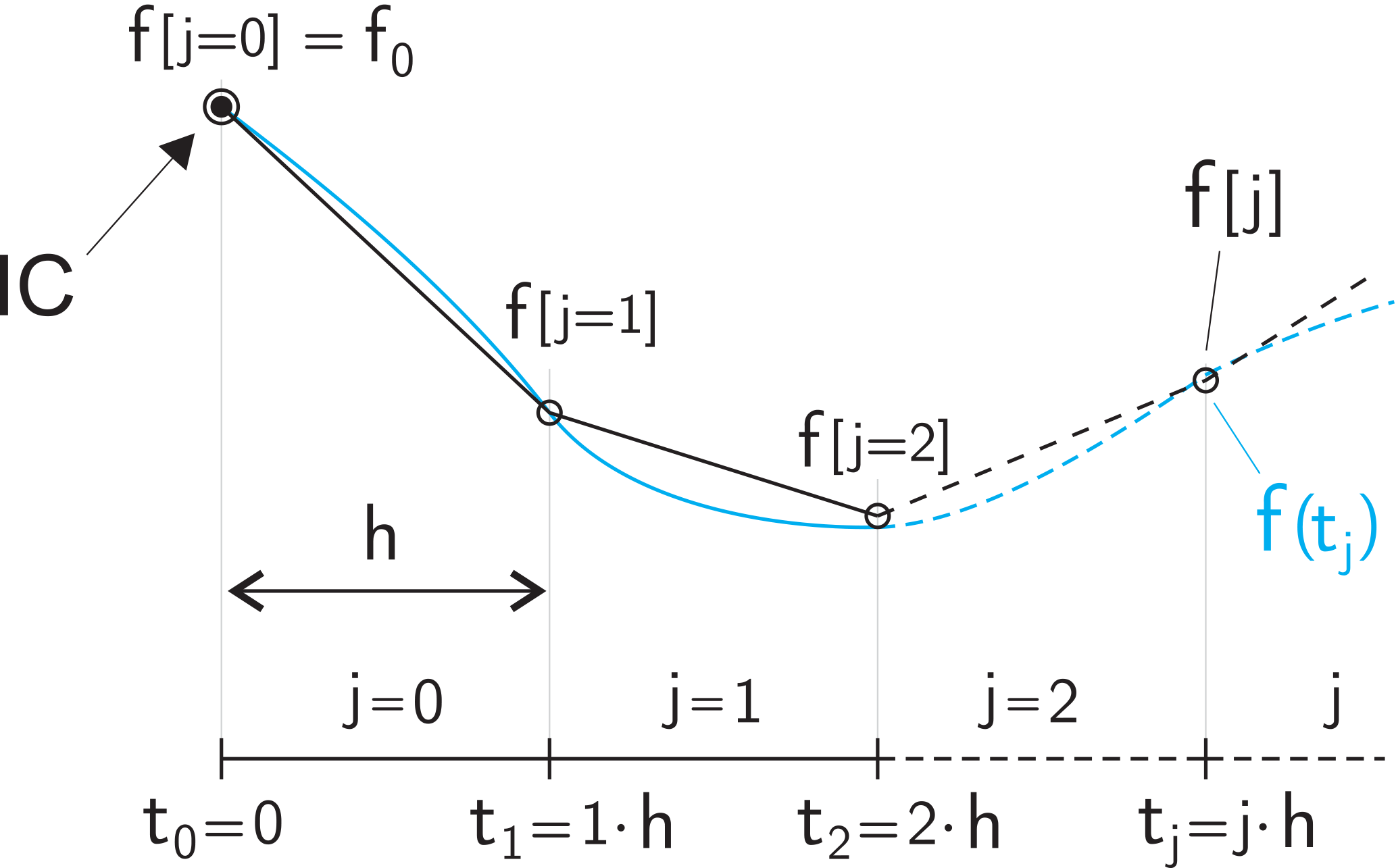
Figure 2Illustration of the conventions used to discretize the time domain. Time steps have a fixed length h (e.g., 12 h) and each time step j starts in . The numerical evaluation of a function f at time tj is indicated as f[j].
To solve Eq. (8), we implement a forward Euler scheme. This explicit numerical scheme is intuitive and fast to solve, and its numerical accuracy is shown to be satisfactory for many hydrologic applications (see model verification, Sect. 5.1). By terming , the discretized problem becomes
for , with N indicating the number of time steps in the simulation, and boundary condition . In a pure forward Euler scheme, this boundary condition implies that , meaning that no input can be part of an output during the same time step. This can be a limitation for catchment applications, where “event” water is often not negligible and it can bear important information on catchment form and function. For this reason, in Eq. (9) we use a modified Ω* defined as
where e[j] is an estimate of the youngest water stored in the system at the end of time step j. Such an estimate is obtained here as , i.e., it is a water balance for current precipitation input using the SAS functions evaluated at a previous time step. The classic Euler scheme is returned if e[j]=0. This modification of the classic numerical scheme only affects the behavior of the youngest age in the system and it is a simple and efficient way to account for transport of event water. The accuracy of this numerical scheme is evaluated in Sect. 5.1.
3.2 Numerical routine
The model solves Eq. (9) by implementing an external for-loop on j (i.e., on the chronological time) and an internal for-loop on i (i.e., on the ages). This means that during one time step j all the characteristic curves (Eq. 9) are updated by one time step. The internal loop is implemented using vector operations. The vector length is indicated as nj and it depends on the number of age classes (which is also the number of characteristic curves) that are included in the computations at time j (see Sect. 3.3). At any time step, the two fundamental operations to solve the discretized ME are
To compute the model output, further operations are required. In particular,
-
update , which is valid for conservative solutes entering through precipitation;
-
compute ;
-
compute .
Starting from these basic routines, many additional operations can be implemented to, for example, characterize the nonconservative behavior of solutes or to compute some age distribution statistics.
3.3 Additional numerical details
A first issue that the model needs to take into account is that age distributions are defined over an age domain , meaning that the rank storage is made of an infinite number of elements where the oldest elements typically represent infinitesimal stored volumes. To have a finite number of elements in the computations, an arbitrary old fraction of rank storage can be considered as a single undifferentiated volume of “older” water. This allows us to merge a high number of very little residual volumes into a single old pool. Note that the term old should be used carefully as its definition depends on the particular system under consideration and it may differ depending on the characteristic timescales of the solute used to infer water age (Benettin et al., 2017a). The old pool is defined here as the volume , where Sth is a numerical parameter that can be fixed for each different application. Sth also defines the age Tth, corresponding to , which indicates the oldest age that is computed individually. Numerically, the parameter Sth controls the number nj of age classes (or equivalently rank storage volumes) that are taken into account in the computations. Sth should be chosen so that the number of elements used in the computations remains small but the numerical accuracy is not compromised. It can be convenient to define a nondimensional threshold such that Sth=fth S(t). In this case, a value fth=0.9 means that the old pool comprises the oldest 10 % of the water storage. When fth=1 no old pool is taken into account. Once a storage element is merged to the old pool, its individual age and concentration properties cannot be retrieved, but the mean properties of the old pool like the mean solute concentration are preserved.
A second, connected problem regards the initial conditions of the system, i.e., the unknown storage age distribution and solute concentration to be used at the beginning of the calculations. In the absence of information, the initial storage can be considered as one single old pool; hence the initial number of age classes n0 is equal to 1. Once computations start, new elements are introduced and accounted for in the balance, reducing the impact and the influence of the initial conditions. The old pool gets progressively smaller (and vector length nj larger) until it reaches the stationary value defined by Sth. An initial spinup period can be used to initialize the ME balance and reduce the size of the initial old water pool. This is particularly indicated when modeling solutes with long turnover times like tritium. The influence of the initial conditions decreases with time, but given the long timescales that may characterize transport processes, it is likely never completely exhausted. This has little impact on the output concentration but it limits the maximum computable age to the time elapsed since the start of the simulation.
The computational time of a simulation can be reduced by not accounting for zero-precipitation inputs as they have no influence in the balance but increase the number of operations required at each time step. In such a case, however, the position of an element in the vector does not correspond with its age anymore and age has to be counted separately. To keep the model intuitive, we decided to not remove zero-precipitation inputs.
Application of the approach requires knowledge of the input or output water fluxes to or from the catchment, the input solute concentration, and the initial conditions for the water storage magnitude and concentration. Then, an SAS function must be specified for each outflow. The code comes with example virtual data that can be used to evaluate the model capabilities. Hydrologic data for 4 years were obtained from recorded precipitation and streamflow at the Mebre-Aval catchment near Lausanne (CH). Evapotranspiration was obtained from regional daily estimates around the Lausanne area and modified to match the long-term mass balance. On average, yearly precipitation is 1100 mm, discharge is 580 mm (53 % of precipitation) and evapotranspiration is 520 mm. The storage variations, computed by solving the hydrologic balance, were normalized to the interval [0,1] to serve as a nondimensional metric of catchment wetness (variable wi). Overall, the data are not meant to be representative of a particular location, but they constitute a realistic set of hydrologic variables to test the model.
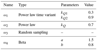
The code was run on the example data using the four illustrative shapes for the discharge SAS function listed in Table 1. All simulations share the following settings: 12 h time step, 4-year spinup period obtained by repeating the example data, storage threshold fth=1 (i.e., no old-pool schematization), initial storage parameter S0=1000, and evapotranspiration SAS function selected as a power law with parameter k=1 (equivalent to a random sampling). The different shapes for the discharge SAS function were selected to test different functional forms (power law, power law time variant, beta distribution) and to illustrate the transition from the preferential release of younger water volumes (examples ω1 and ω2) to the random sampling case (ω3) and the preferential release of older waters (ω4). The time-variant power-law SAS (ω1) was obtained by using Eq. (6) with a time-variant exponent , with parameters kQ1 and kQ2 corresponding to the exponent k during the wettest (wi =1) and driest (wi =0) conditions. This parameter choice is used for illustration purposes and should not be taken as representative of a general catchment behavior.
Table 1Description of the discharge SAS functions used in the application. All the functions were tested with the same initial total storage S0=1000 mm.
Two different examples of solute transport were simulated in the test. In the first case, solute input concentration was generated by adding noise to a sinusoidal wave with an annual cycle. This example can be representative of atmospheric tracers with a yearly period (like stable water isotopes). In the second case, the initial storage was set to a concentration of 100 mg L−1 and any subsequent input was assigned a concentration of 0 mg L−1, causing the system to dilute. This example can be representative of a diluting system, e.g., a catchment with conservative agricultural inputs like chloride (Martin et al., 2004; van der Velde et al., 2010) that undergoes a step reduction. Results of both examples are shown in Fig. 3.
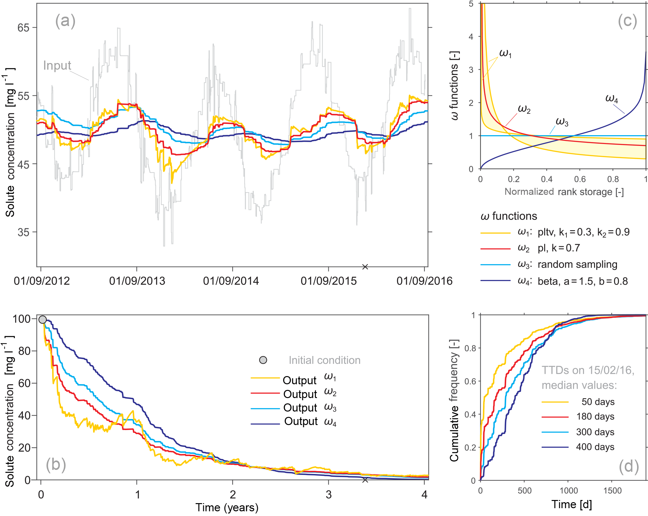
Figure 3Example of results that can be obtained from the model. (a) Streamflow solute response in the case of sinusoidal tracer input; (b) streamflow solute response in the case of step reduction of the tracer input; (c) illustration of the different ωQ used in the simulations and listed in Table 1 (as ω1 is time variant; its possible shapes are represented by a colored band); (d) cumulative streamflow travel time distributions (TTDs) extracted on a specific day (15 February 2016, indicated with a cross in a and b). All simulations share the same settings and only differ in the choice of the ωQ function.
Each discharge SAS function simulates different transport mechanisms and provides rather different outputs, both in terms of water age and streamflow concentration. In the first solute transport example (Fig. 3a), discharge concentration gets progressively damped and shifted as the SAS function moves from younger-water preference to older-water preference. The travel time distributions extracted for 15 February 2016 (Fig. 3d) show that the median age of streamflow may vary by a factor of 3–8 simply based on the selection of the SAS function (i.e., leaving the storage parameter unchanged). The affinity for younger water is rather typical in catchments, at least during wet conditions, while the release of older water is more representative of soil columns or aquifers. The second solute example (Fig. 3b) evaluates the “memory” of a system, i.e., the time needed to adapt to a new condition. Again, the preferential release of older storage volumes and the implied lack of young water in streamflow makes the system response more damped. However, this also means that the old water gets depleted faster; hence in the long term the trend may be reversed and the residual legacy of the initial conditions may be stronger in systems with a high affinity for younger water. This is visible in Fig. 3b right after year 2, although the effect is very mild in this case. The time-variant SAS function (ω1) is particularly illustrative in this example because it shows that streamflow concentration can increase in time (e.g., around year 1 in Fig. 3b), even in the absence of new solute input, just as a consequence of the changing transport mechanisms.
Overall, these quick examples were used to illustrate the model capabilities and to show that results may change significantly depending on the choice of the parameters. A sensitivity analysis is generally advised to identify the parameters that have the highest impact on model results. For example, previous catchment studies (e.g., Benettin et al., 2017b) highlighted the challenge in constraining the SAS function of ET flux when based on streamflow concentration measurements only. As a consequence, the hypothesis of random sampling for the ET flux is often as valid as the preference for the younger or older stored water, but it is more parsimonious. Different model outputs are affected by parameters in different ways, and water ages (for example the median age, Fig. 3d) are typically more sensitive than solute concentration to parameter variations. The low computational times of the model aid the development of sensitivity analyses.
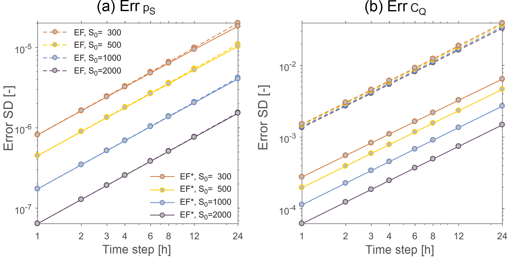
Figure 4Numerical errors on the storage age distribution (a) and on streamflow concentration (b) as a function of the aggregation time step. The error time series are summarized through their standard deviation (SD). Each plot shows the performance of two different numerical schemes: classic Euler forward (EF) and modified Euler forward (EF*, which is the default model version). The EF* implementation shows significant improvements with respect to EF in the accuracy of streamflow concentration.
5.1 Model verification
Here we evaluate the numerical accuracy of the model in computing the solution of the age ME (i.e., the rank storage ST) and streamflow concentration CQ. The numerical model is first evaluated by comparing our modified Euler solution (Eq. 9) to a numerical implementation of the analytic solution (Eq. 1). This comparison is only possible for the case of random sampling (see Sect. 2.4), as no analytic solution is usually available for other transport schemes. Then, the comparison is made for other shapes of the SAS function, approximating the true solution with a higher-order implementation of Eq. (8). As in Sect. 4, comparisons are made on the example dataset, using daily average fluxes and the sinusoidal tracer input concentration.
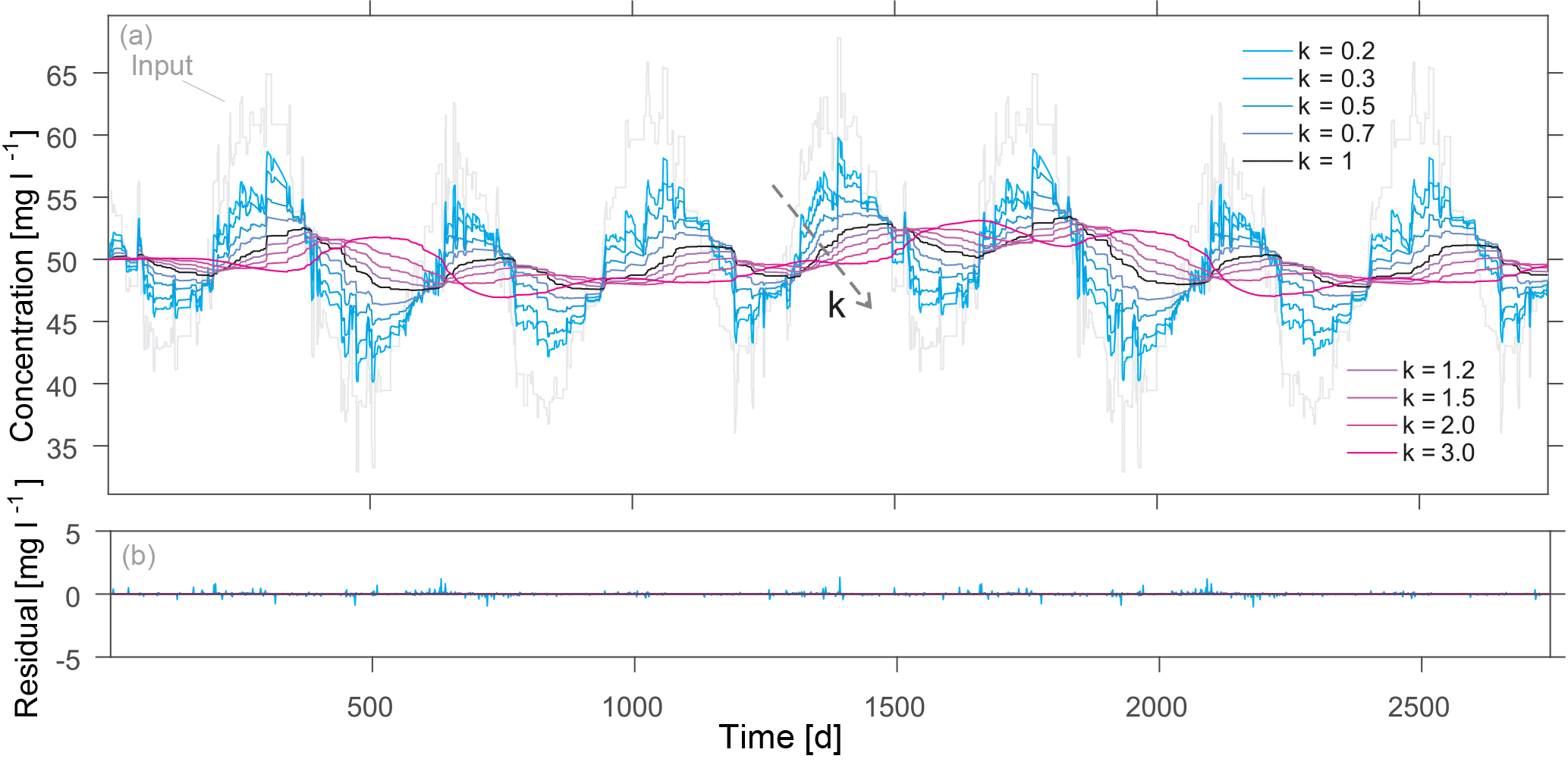
Figure 5Solute concentration (CQ) time series obtained from power-law SAS functions with parameter S0=1000 and parameter , using a 24 h time step (a). The time series are rather different, as they are progressively more lagged and damped for increasing values of k. The difference with the higher-order solution forms the residual time series (b, same scale as a). Residuals are overall limited and they do not cumulate during the 8-year simulation.
For the RS comparison, the analytic solution was obtained by implementing Eq. (7) at a daily scale, considering that fluxes are piecewise constant while the storage is piecewise linear during the time step. The numerical solution for the RS was obtained by setting both ΩQ and ΩET as power laws with parameters . The numerical model was run for eight different aggregation time steps h: 1, 2, 3, 4, 6, 8, 12 and 24 h. For each run, the resulting streamflow concentration and one rank storage (corresponding to the end of day 2745) were used for comparison with the analytic solution. Models were run for 8 years using 4 years of spinup. To allow direct comparisons across different aggregation time steps, streamflow concentrations were extracted at the end of each day, resulting in eight different time series (one per h) of 2920 elements. The time series were then normalized by the mean and standard deviation of the analytic solution. A time series of model errors on streamflow concentration (err) was finally obtained from the difference between the analytic and the numerical (normalized) solutions. The rank storage was evaluated on the entire age domain every 24 h (again, to allow comparisons across different time steps). To avoid comparisons between cumulative functions, the rank storage was used to compute the storage age probability density function pS (see Sect. 2.1). The errors on pS were obtained from the difference between the analytic and the numerical solutions. In this case, the error time series (err) consists, for each of the eight aggregation time steps, of 2745 elements. For additional comparisons, the performance of our numerical implementation (EF*) was compared to the classic implementation of the forward Euler scheme (EF, i.e., Eq. (10) with e[j]=0). Results are obtained for four different values of the initial storage S0: 300, 500, 1000 and 2000 mm. The standard deviations of err and err are shown in Fig. 4 as a function of the aggregation time step. The EF and EF* implementations almost have the same error on pS, indicating that accounting for the event water does not have a major impact on the overall solution of the age ME. However, as different ages do not contribute equally to streamflow, the event water can have a larger impact on streamflow concentration. This is evident in the performance on err, where the modified EF* implementation is about 1 order of magnitude more accurate than the classic Euler scheme. The error is on average smaller than 10−2 the variance of the CQ signal, which is lower than most measurement errors. The performance on err also shows that the errors tend to grow with decreasing values of the mean storage, i.e., when the storage gets depleted (or filled) faster. The error of the EF* scheme shows a good stability. This is not surprising as the RS case resembles a linear reservoir (see Sect. 2.4) with a coefficient c approximately equal to the mean ratio between the fluxes and the storage 〈J∕S〉 during a time step. The stability condition for the Euler forward scheme in the case of a linear reservoir requires that (no fast decay). In typical hydrologic applications, fluxes are usually much smaller than the storage; hence and the EF solution is stable.
Results show that the numerical implementation of the ME is satisfactory for the RS solution in terms of both accuracy and stability. However, solutions other than the RS case may be more challenging owing to the nonuniform age selection played by the outflows. For this reason, we tested power-law SAS functions (Eq. 6) with different values of the exponent k: 0.2, 0.3, 0.5, 0.7, 1, 1.2, 1.5, 2 and 3. The same exponent was used each time for both ΩQ and ΩET. The model was run with a fixed initial storage S0=1000, for the same timespan and aggregation time steps as in the RS case, and the performance was again evaluated in terms of err and err. Given the lack of analytical solutions, we approximated the true solution by using a higher-order implementation (built-in MATLAB solver “ode113”; Shampine and Reichelt, 1997) for Eq. (8). An example of the CQ time series obtained from the different values of k for h=24 h is reported in Fig. 5. The CQ time series are rather different, being progressively more lagged and damped for increasing values of k. Although the residual with respect to the higher-order solution can occasionally be up to 1.3 mg L−1, it is on average very low compared to the signal. Thus in this case the accuracy of the model is satisfactory even for h=24 h. Note that for this dataset, the parameters of the SAS function (k=0.2 and S0=1000) imply that 30 % of the input, on average, becomes output during the same day. The residuals are overall low and do not accumulate during the 8-year simulation, suggesting that even the 24 h simulation is stable. The performance on CQ was further evaluated in the same way as for the RS case: we normalized the concentration signals and obtained the error time series err from the difference with the higher-order solution. Similarly, we computed the errors err with respect to the higher-order solution for simulation day 2745.
The standard deviations of the errors are shown in Fig. 6 for different values of k and aggregation time steps. The errors on pS grow for increasing preference of the SAS functions for the younger stored volumes (lower values of k). This indicates that the young water preference is a more challenging numerical condition for the solution of the age ME. This behavior is to be mostly attributed to the errors on the youngest waters in storage. Although we use a modified version of the EF scheme to account for the presence of event water in the outflows (Eq. 10), this approximation has some limitations. In particular, the youngest age in storage (e[j]) is quantified through the SAS function from previous time step; thus it may give rise to errors at the onset of intense storm events. The interpretation of the behavior of the error on CQ (Fig. 6b) is less straightforward as the errors on the solution pS can be amplified in various ways by the different SAS functions. Errors appear not too dissimilar for k in the range 0.5–1.2 and they are all reduced by 1 order of magnitude moving from daily to hourly time steps. The more extreme age selections (i.e., k≤0.3 and k≥2) tend to result in higher errors, although the error magnitude remains low (less than 10−2 the signal variance) and the solution is stable.
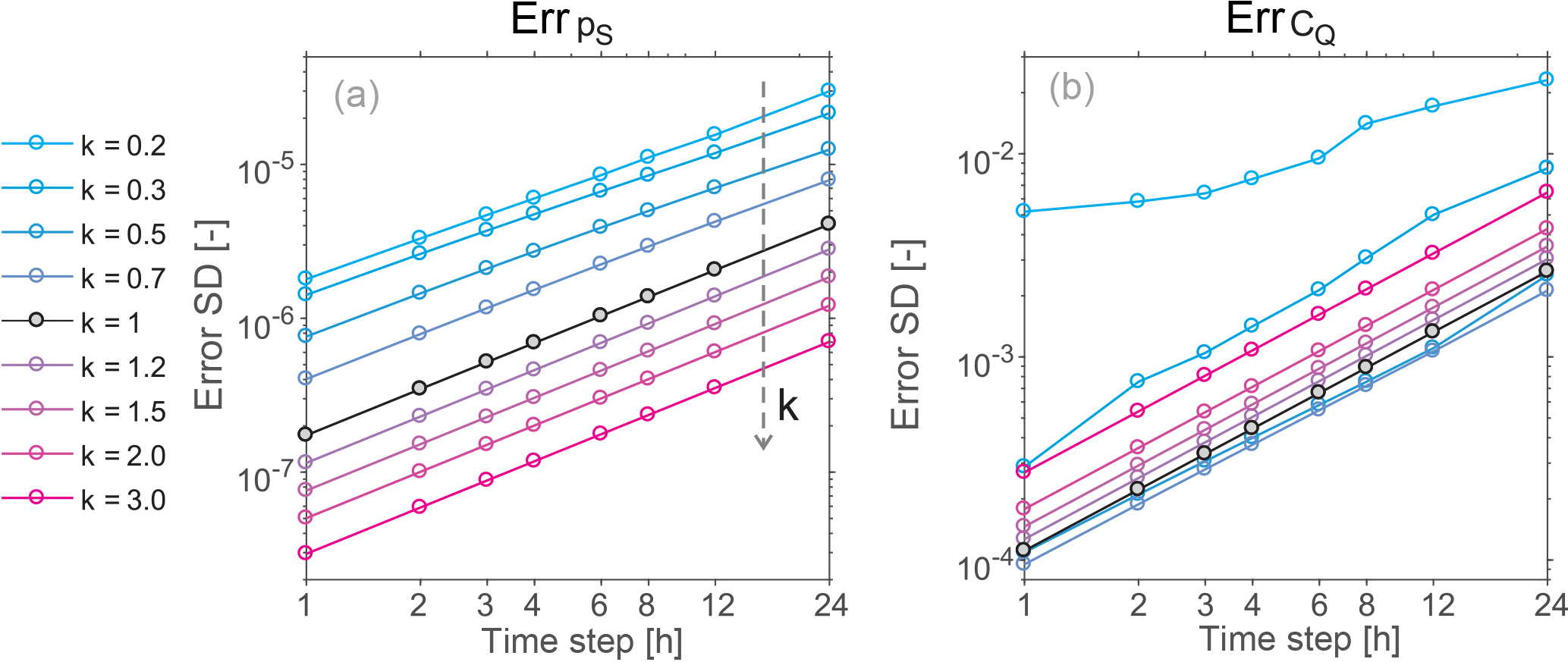
Figure 6Numerical errors on the storage age distribution (a) and on streamflow concentration (b) as a function of the aggregation time step. The error time series are summarized through their standard deviation. Each plot shows the model performance for several shapes of the SAS function, parameterized as a power-law distribution with parameter k (Eq. 6). The color code is the same as in Fig. 5. The random-sampling case (i.e., k=1) is indicated in black and it is equivalent to the curves featuring S0=1000 in Fig. 4.
These examples suggest that the behavior of the system can be interpreted using a (nonlinear) reservoir analogy. Each individual water parcel can be seen as a depleting reservoir that decreases in time owing to the particular outflow removal (Eq. 8). This removal is mediated by the SAS functions; thus it can become large corresponding to high values of ω(ST,t), potentially leading to an unstable fast decay. The depletion pattern of the reservoir is rather complex as it is nonlinear and it changes at every time step, but it suggests that very pronounced age selections should be considered carefully and checked for potential numerical instabilities. Note that for illustration purposes the effects of the two power-law SAS function parameters k and S0 were presented separately (Figs. 4 and 6), but they should be considered together as lower storage values may enhance the selection of younger or older waters and increase the numerical errors. The model was tested here for several shapes of the SAS functions on a realistic hydrochemical dataset. Although every dataset is different and it would be impossible to perform a model verification valid for all applications, these results provide some first guidelines as to where the explicit numerical implementation may become critical.
5.2 Model applicability, limitations and perspectives
The model is based on a catchment-scale approach, so it only requires catchment-scale fluxes like precipitation, discharge and evapotranspiration. These fluxes can often be measured (or modeled in the case of ET) without the need for a full hydrologic model. Moreover, the pure SAS function approach implies that, differently from previous approaches (e.g., Bertuzzo et al., 2013; Benettin et al., 2015a), the transport equations which are solved in the model are completely decoupled from the way fluxes were obtained. This notably reduces the number of involved parameters and it simplifies the applicability of the model to different datasets and contexts. Although more research is needed to classify the expected shapes of the SAS functions based on measurable catchment properties, one can quickly obtain first-order evaluations of solute transport by using SAS functions already tested in the literature (e.g., van der Velde et al., 2015; Harman, 2015; Queloz et al., 2015b; Benettin et al., 2017b; Wilusz et al., 2017) and a reasonable choice of the initial storage S0.
The use of an explicit numerical scheme has the potential of greatly reducing the computational times. Short aggregation time steps are generally recommended, especially when testing the affinity for younger storage volumes (e.g., Eq. (6) with parameter k<0.3), but in case larger time steps (e.g., h=24 h) prove satisfactory, the model can typically run in less than a second on a normal computer. The short computational times make the use of calibration techniques easier and the model structure is directly compatible with the DREAM (Vrugt et al., 2009; ter Braak and Vrugt, 2008) calibration packages. The model can be made faster by not considering the zero-precipitation times but, as explained in Sect. 3.3, this improvement is currently not implemented to keep the model more intuitive.
The model is based on a catchment-scale formulation of transport processes; thus it cannot provide spatial information unless the system is partitioned into a series of spatial compartments (e.g., Soulsby et al., 2015). Even in this case, one would need to know the fluxes to and from each compartment, hence losing one of the main advantages of the general SAS approach. The catchment-scale nature of the formulation also implies that SAS functions have a conceptual character and they cannot be determined directly from physical properties of the system. Their general shape, however, can be traced back to elementary advection–dispersion processes (Benettin et al., 2013) and the mechanistic basis for time-variable SAS functions has recently been highlighted (Pangle et al., 2017).
Although the numerical accuracy of the computations has to be evaluated for each different application, Sect. 5.1 provides some first guidelines to cases in which the numerical accuracy may not be satisfactory. Systems whose storage is quickly depleted by the fluxes are prone to inaccuracies and instabilities. This can happen, for instance, if the system storage is small compared to the fluxes and the SAS functions have a very strong preference for some storage portions. In such cases, higher-order schemes may become desirable. The model package already provides a higher-order solution to Eq. (8) (obtained through the MATLAB built-in function “ode113”) that can help evaluate the numerical accuracy of the results.
The codes implemented in the tran-SAS package can be used to simulate the transport of conservative solutes through a catchment. This represents a first step towards the modeling of large-scale solute transport. Simple reactive transport equations can be easily implemented in the main model routine (Sect. 3.2) using effective formulations that integrate biogeochemical processes across the catchment heterogeneity (Rinaldo and Marani, 1987). Being based on a travel time formulation of transport, the model is obviously not suited to simulating the circulation of solutes for which the chronology of the inputs and the age of water are irrelevant. For a number of cases of interest, however, both the time of entry into the catchment and the residence time of water within the catchment storage may play an important role in the transport process. Many such examples have been addressed in the literature using a catchment-scale approach, including the case of nitrate export from agricultural catchments (Botter et al., 2006; van der Velde et al., 2012), solutes influenced by evapoconcentration effects (Queloz et al., 2015b), pesticide transport (Bertuzzo et al., 2013; Lutz et al., 2017) and solutes produced by mineral weathering (Benettin et al., 2015a). The provided codes are designed to be easy to understand, so that they can be easily customized by the user and adapted to different contexts and applications. The next step is then to adapt the model to real-world problems, for which solutes' nonconservative behavior has to be taken into account.
The tran-SAS package includes a basic implementation of the age master equation (Eq. 1) using general SAS functions. The codes can be used to simulate the transport of solutes through a catchment and to evaluate water residence times. The package is ready to go and it includes some example data that can be used to test the main model features. The codes are extensively commented on so that they can be edited according to the user's needs. The model is based on a catchment-scale formulation of solute transport and it only relies on measurable data. Main model equations are implemented using an explicit Euler scheme that allows us to reduce computational times. The numerical accuracy of the model was verified on the example data and was shown to be generally satisfactory even at larger (e.g., daily) computation time steps. The most critical cases are those in which the stored water parcels are rapidly removed by the outflows. This situation can occur when the SAS function assumes very high values for some stored water volumes. In such cases, higher-order model implementations (provided within the package) should be used to check the numerical accuracy of the solution. The model allows us to test different SAS functions and evaluate solute transport in the catchment storage and outflows. Applications can be oriented to different catchments and solutes, advancing our ability to understand and model catchment transport processes.
The current model release, including example data and documentation, is available at https://doi.org/10.5281/zenodo.1203600. A maintained GitHub project is available at the following GitHub repository: https://github.com/pbenettin/tran-SAS.
The authors declare that they have no conflict of interest.
The authors thank Andrea Rinaldo and Gianluca Botter for the useful
discussions that inspired this work and Damiano Pasetto for support in the
numerical implementation of the model equations. Paolo Benettin thanks the
ENAC school at EPFL for financial support.
Edited by: Jeffrey Neal
Reviewed by: three anonymous referees
Benettin, P., Rinaldo, A., and Botter, G.: Kinematics of age mixing in advection-dispersion models, Water Resour. Res., 49, 8539–8551, https://doi.org/10.1002/2013WR014708, 2013. a
Benettin, P., Bailey, S. W., Campbell, J. L., Green, M. B., Rinaldo, A., Likens, G. E., McGuire, K. J., and Botter, G.: Linking water age and solute dynamics in streamflow at the Hubbard Brook Experimental Forest, NH, USA, Water Resour. Res., 51, 9256–9272, https://doi.org/10.1002/2015WR017552, 2015a. a, b
Benettin, P., Rinaldo, A., and Botter, G.: Tracking residence times in hydrological systems: forward and backward formulations, Hydrol. Proc., 29, 5203–5213, https://doi.org/10.1002/hyp.10513, 2015b. a, b
Benettin, P., Bailey, S. W., Rinaldo, A., Likens, G. E., McGuire, K. J., and Botter, G.: Young runoff fractions control streamwater age and solute concentration dynamics, Hydrol. Proc., 31, 2982–2986, https://doi.org/10.1002/hyp.11243, 2017a. a
Benettin, P., Soulsby, C., Birkel, C., Tetzlaff, D., Botter, G., and Rinaldo, A.: Using SAS functions and high resolution isotope data to unravel travel time distributions in headwater catchments, Water Resour. Res., 53, 1864–1878, https://doi.org/10.1002/2016WR020117, 2017b. a, b, c, d
Bertuzzo, E., Thomet, M., Botter, G., and Rinaldo, A.: Catchment-scale herbicides transport: Theory and application, Adv. Water Resour., 52, 232–242, https://doi.org/10.1016/j.advwatres.2012.11.007, 2013. a, b
Botter, G.: Catchment mixing processes and travel time distributions, Water Resour. Res., 48, W05545, https://doi.org/10.1029/2011WR011160, 2012. a
Botter, G., Settin, T., Marani, M., and Rinaldo, A.: A stochastic model of nitrate transport and cycling at basin scale, Water Resour. Res., 42, W04415, https://doi.org/10.1029/2005WR004599, 2006. a
Botter, G., Bertuzzo, E., Bellin, A., and Rinaldo, A.: On the Lagrangian formulations of reactive solute transport in the hydrologic response, Water Resour. Res., 41, W04008, https://doi.org/10.1029/2004WR003544, 2005. a
Botter, G., Bertuzzo, E., and Rinaldo, A.: Catchment residence and travel time distributions: The master equation, Geophys. Res. Lett., 38, L11403, https://doi.org/10.1029/2011GL047666, 2011. a, b, c, d, e
Calabrese, S. and Porporato, A.: Linking age, survival, and transit time distributions, Water Resour. Res., 51, 8316–8330, https://doi.org/10.1002/2015WR017785, 2015. a
Cvetkovic, V. and Dagan, G.: Transport of kinetically sorbing solute by steady random velocity in heterogeneous porous formations, J. Fluid Mech., 265, 189–215, https://doi.org/10.1017/S0022112094000807, 1994. a
Danesh-Yazdi, M., Foufoula-Georgiou, E., Karwan, D. L., and Botter, G.: Inferring changes in water cycle dynamics of intensively managed landscapes via the theory of time-variant travel time distributions, Water Resour. Res., 52, 7593–7614, https://doi.org/10.1002/2016WR019091, 2016. a, b
Danesh-Yazdi, M., Botter, G., and Foufoula-Georgiou, E.: Time-variant Lagrangian transport formulation reduces aggregation bias of water and solute mean travel time in heterogeneous catchments, Geophys. Res. Lett., 44, 4880–4888, https://doi.org/10.1002/2017GL073827, 2017. a
Destouni, G., Persson, K., Prieto, C., and Jarsjö, J.: General Quantification of Catchment-Scale Nutrient and Pollutant Transport through the Subsurface to Surface and Coastal Waters, Environ. Sci. Technol., 44, 2048–2055, https://doi.org/10.1021/es902338y, 2010. a
Drever, M. C. and Hrachowitz, M.: Migration as flow: using hydrological concepts to estimate the residence time of migrating birds from the daily counts, Methods Ecol. Evol., 8, 1146–1157, https://doi.org/10.1111/2041-210X.12727, 2017. a, b
Harman, C. J.: Time-variable transit time distributions and transport: Theory and application to storage-dependent transport of chloride in a watershed, Water Resour. Res., 51, 1–30, https://doi.org/10.1002/2014WR015707, 2015. a, b, c, d, e, f, g, h
Harman, C. J., Ward, A. S., and Ball, A.: How does reach-scale stream-hyporheic transport vary with discharge? Insights from rSAS analysis of sequential tracer injections in a headwater mountain stream, Water Resour. Res., 52, 7130–7150, https://doi.org/10.1002/2016WR018832, 2016. a
Hrachowitz, M., Fovet, O., Ruiz, L., and Savenije, H. H. G.: Transit time distributions, legacy contamination and variability in biogeochemical 1∕fα scaling: how are hydrological response dynamics linked to water quality at the catchment scale?, Hydrol. Proc., 29, 5241–5256, https://doi.org/10.1002/hyp.10546, 2015. a
Hrachowitz, M., Benettin, P., Breukelen, B. M. V., Fovet, O., Howden, N. J. K., Ruiz, L., Velde, Y. V. D., and Wade, A. J.: Transit times –the link between hydrology and water quality at the catchment scale, WIRES Water, 3, 629–657, https://doi.org/10.1002/wat2.1155, 2016. a
Jackson, B., Wheater, H., Wade, A., Butterfield, D., Mathias, S., Ireson, A., Butler, A., McIntyre, N., and Whitehead, P.: Catchment-scale modelling of flow and nutrient transport in the Chalk unsaturated zone, Ecol. Model., 209, 41–52, https://doi.org/10.1016/j.ecolmodel.2007.07.005, 2007. a
Kauffman, S. J., Royer, D. L., Chang, S., and Berner, R. A.: Export of chloride after clear-cutting in the Hubbard Brook sandbox experiment, Biogeochemistry, 63, 23–33, https://doi.org/10.1023/A:1023335002926, 2003. a
Kim, M., Pangle, L. A., Cardoso, C., Lora, M., Volkmann, T. H. M., Wang, Y., Harman, C. J., and Troch, P. A.: Transit time distributions and StorAge Selection functions in a sloping soil lysimeter with time-varying flow paths: Direct observation of internal and external transport variability, Water Resour. Res., 52, 7105–7129, https://doi.org/10.1002/2016WR018620, 2016. a, b
Lutz, S. R., Velde, Y. V. D., Elsayed, O. F., Imfeld, G., Lefrancq, M., Payraudeau, S., and van Breukelen, B. M.: Pesticide fate on catchment scale: conceptual modelling of stream CSIA data, Hydrol. Earth Syst. Sci., 21, 5243–5261, https://doi.org/10.5194/hess-21-5243-2017, 2017. a
Maher, K.: The role of fluid residence time and topographic scales in determining chemical fluxes from landscapes, Earth Planet. Sc. Lett., 312, 48–58, https://doi.org/10.1016/j.epsl.2011.09.040, 2011. a
Maloszewski, P. and Zuber, A.: Principles and practice of calibration and validation of mathematical models for the interpretation of environmental tracer data in aquifers, Adv. Water Resour., 16, 173–190, https://doi.org/10.1016/0309-1708(93)90036-F, 1993. a
Martin, C., Aquilina, L., Gascuel-Odoux, C., Molénat, J., Faucheux, M., and Ruiz, L.: Seasonal and interannual variations of nitrate and chloride in stream waters related to spatial and temporal patterns of groundwater concentrations in agricultural catchments, Hydrol. Proc., 18, 1237–1254, https://doi.org/10.1002/hyp.1395, 2004. a
McGuire, K. J. and McDonnell, J. J.: A review and evaluation of catchment transit time modeling, J. Hydrol., 330, 543–563, https://doi.org/10.1016/j.jhydrol.2006.04.020, 2006. a
McGuire, K. J. and McDonnell, J. J.: Hydrological connectivity of hillslopes and streams: Characteristic time scales and nonlinearities, Water Resour. Res., 46, W10543,https://doi.org/10.1029/2010WR009341, 2010. a
McMillan, H., Tetzlaff, D., Clark, M., and Soulsby, C.: Do time-variable tracers aid the evaluation of hydrological model structure? A multimodel approach, Water Resour. Res., 48, W05501, https://doi.org/10.1029/2011WR011688, 2012. a
Oda, T., Asano, Y., and Suzuki, M.: Transit time evaluation using a chloride concentration input step shift after forest cutting in a Japanese headwater catchment, Hydrol. Proc., 23, 2705–2713, https://doi.org/10.1002/hyp.7361, 2009. a
Pangle, L. A., Kim, M., Cardoso, C., Lora, M., Meira Neto, A. A., Volkmann, T. H. M., Wang, Y., Troch, P. A., and Harman, C. J.: The mechanistic basis for storage-dependent age distributions of water discharged from an experimental hillslope, Water Resour. Res., 53, 2733–2754, https://doi.org/10.1002/2016WR019901, 2017. a
Queloz, P., Bertuzzo, E., Carraro, L., Botter, G., Miglietta, F., Rao, P., and Rinaldo, A.: Transport of fluorobenzoate tracers in a vegetated hydrologic control volume: 1. Experimental results, Water Resour. Res., 51, 2773–2792, https://doi.org/10.1002/2014WR016433, 2015a. a
Queloz, P., Carraro, L., Benettin, P., Botter, G., Rinaldo, A., and Bertuzzo, E.: Transport of fluorobenzoate tracers in a vegetated hydrologic control volume: 2. Theoretical inferences and modeling, Water Resour. Res., 51, 2793–2806, https://doi.org/10.1002/2014WR016508, 2015b. a, b, c, d, e
Rigon, R., Bancheri, M., and Green, T. R.: Age-ranked hydrological budgets and a travel time description of catchment hydrology, Hydrol. Earth Syst. Sci., 20, 4929–4947, https://doi.org/10.5194/hess-20-4929-2016, 2016. a
Rinaldo, A. and Marani, A.: Basin scale-model of solute transport, Water Resour. Res., 23, 2107–2118, https://doi.org/10.1029/WR023i011p02107, 1987. a, b
Shampine, L. F. and Reichelt, M. W.: The MATLAB ODE Suite, SIAM J. Sci. Comput., 18, 1–22, https://doi.org/10.1137/S1064827594276424, 1997. a
Soulsby, C., Birkel, C., Geris, J., and Tetzlaff, D.: Spatial aggregation of time-variant stream water ages in urbanizing catchments, Hydrol. Proc., 29, 3038–3050, https://doi.org/10.1002/hyp.10500, 2015. a
ter Braak, C. J. F. and Vrugt, J. A.: Differential Evolution Markov Chain with snooker updater and fewer chains, Stat. Comput., 18, 435–446, https://doi.org/10.1007/s11222-008-9104-9, 2008. a
van der Velde, Y., Heidbüchel, I., Lyon, S. W., Nyberg, L., Rodhe, A., Bishop, K., and Troch, P. A.: Consequences of mixing assumptions for time-variable travel time distributions, Hydrol. Proc., 29, 3460–3474, https://doi.org/10.1002/hyp.10372, 2015. a, b, c
van der Velde, Y., de Rooij, G. H., Rozemeijer, J. C., van Geer, F. C., and Broers, H. P.: Nitrate response of a lowland catchment: On the relation between stream concentration and travel time distribution dynamics, Water Resour. Res., 46, W11534, https://doi.org/10.1029/2010WR009105, 2010. a
van der Velde, Y., Torfs, P. J. J. F., van der Zee, S. E. A. T. M., and Uijlenhoet, R.: Quantifying catchment-scale mixing and its effect on time-varying travel time distributions, Water Resour. Res., 48, W06536, https://doi.org/10.1029/2011WR011310, 2012. a, b, c, d, e
Vrugt, J., Braak, C. T., Diks, C., Robinson, B., Hyman, J., and Higdon, D.: Accelerating Markov chain Monte Carlo simulation by differential evolution with self-adaptive randomized subspace sampling, Int. J. Nonlin. Sci. Num., 10, 271–288, https://doi.org/10.1515/IJNSNS.2009.10.3.273, 2009. a
Weiler, M., McGlynn, B. L., McGuire, K. J., and McDonnell, J. J.: How does rainfall become runoff? A combined tracer and runoff transfer function approach, Water Resour. Res., 39, 1315, https://doi.org/10.1029/2003WR002331, 2003. a
Wilusz, D. C., Harman, C. J., and Ball, W. P.: Sensitivity of Catchment Transit Times to Rainfall Variability Under Present and Future Climates, Water Resour. Res., 53, 10231–10256, https://doi.org/10.1002/2017WR020894, 2017. a, b, c, d