the Creative Commons Attribution 4.0 License.
the Creative Commons Attribution 4.0 License.
 | 04 May 2018
The chemistry–climate model ECHAM6.3-HAM2.3-MOZ1.0
Martin G. Schultz
Scarlet Stadtler
Sabine Schröder
Domenico Taraborrelli
Bruno Franco
Jonathan Krefting
Alexandra Henrot
Sylvaine Ferrachat
Ulrike Lohmann
David Neubauer
Colombe Siegenthaler-Le Drian
Sebastian Wahl
Harri Kokkola
Thomas Kühn
Sebastian Rast
Hauke Schmidt
Philip Stier
Doug Kinnison
Geoffrey S. Tyndall
John J. Orlando
Catherine Wespes
The chemistry–climate model ECHAM-HAMMOZ contains a detailed representation of tropospheric and stratospheric reactive chemistry and state-of-the-art parameterizations of aerosols using either a modal scheme (M7) or a bin scheme (SALSA). This article describes and evaluates the model version ECHAM6.3-HAM2.3-MOZ1.0 with a focus on the tropospheric gas-phase chemistry. A 10-year model simulation was performed to test the stability of the model and provide data for its evaluation. The comparison to observations concentrates on the year 2008 and includes total column observations of ozone and CO from IASI and OMI, Aura MLS observations of temperature, HNO3, ClO, and O3 for the evaluation of polar stratospheric processes, an ozonesonde climatology, surface ozone observations from the TOAR database, and surface CO data from the Global Atmosphere Watch network. Global budgets of ozone, OH, NOx, aerosols, clouds, and radiation are analyzed and compared to the literature. ECHAM-HAMMOZ performs well in many aspects. However, in the base simulation, lightning NOx emissions are very low, and the impact of the heterogeneous reaction of HNO3 on dust and sea salt aerosol is too strong. Sensitivity simulations with increased lightning NOx or modified heterogeneous chemistry deteriorate the comparison with observations and yield excessively large ozone budget terms and too much OH. We hypothesize that this is an impact of potential issues with tropical convection in the ECHAM model.
- Article
(5708 KB) -
Supplement
(2746 KB) - BibTeX
- EndNote


Global chemistry–climate models have become indispensable tools for the investigation of interactions between atmospheric chemistry and various aspects of the physical and biogeochemical climate system. In recent years, several coupled models have been developed with varying levels of interaction between Earth system compartments and varying details in their representation of chemical and physical processes (Young et al., 2013; Morgenstern et al., 2017; Young et al., 2018).
Here, we describe and evaluate a new chemistry–climate model based on the general circulation model ECHAM6.3 (Stevens et al., 2013), the Hamburg Aerosol Model (HAM) version 2.3 (Tegen et al., 2018; Stier et al., 2005; Zhang et al., 2012), and the gas-phase tropospheric and stratospheric module MOZ1.0.
ECHAM6.3-HAM2.3-MOZ1.0 (henceforth ECHAM-HAMMOZ) can be run in different configurations: (1) using prescribed fields of surface pressure, divergence, vorticity, and temperature and applying a relaxation technique with time-varying weights (“nudging”); (2) constraining only sea surface temperatures and sea ice concentrations (“AMIP mode”); or (3) fully coupled with ocean and sea ice models. In this study we concentrate on simulations of type 1 as these allow for a more detailed evaluation of the model with observational data and because most current applications of ECHAM-HAMMOZ use this mode. For a discussion on the potential differences in the different configurations the reader is referred to Lamarque et al. (2012).
Earlier versions of ECHAM-HAMMOZ have been used successfully to analyze the impact of heterogeneous reactions on tropospheric ozone chemistry (Pozzoli et al., 2008a) and on aerosol composition (Pozzoli et al., 2008b) over the North Pacific, the influence of African emissions on regional and global tropospheric ozone (Aghedo et al., 2007), the impact of continental pollution outflow on the chemical tendencies of ozone (Auvray et al., 2007), and the impact of Asian aerosol and trace gas emissions on the Asian monsoon (Fadnavis et al., 2013, 2014, 2015). A 25-year reanalysis with ECHAM-HAMMOZ was performed by Pozzoli et al. (2011). In addition, several studies were performed with the aerosol climate model ECHAM-HAM, which uses trace gas climatologies from ECHAM-HAMMOZ to constrain aerosol nucleation (e.g., Jiao et al., 2014; Neubauer et al., 2014; Stanelle et al., 2014; Ghan et al., 2016; Zhang et al., 2016). The tropospheric chemistry–climate model ECHAM5-MOZ also participated in the first multi-model intercomparison study of the Task Force Hemispheric Transport of Air Pollutants (TFHTAP) (Dentener et al., 2006a; Stevenson et al., 2006).
This article intends to provide a thorough description of the chemistry component of the ECHAM-HAMMOZ model with special focus on tropospheric reactive gases. Stratospheric chemistry is briefly discussed as well, while for more detailed discussions of the performance of the physical climate model ECHAM6.3 the reader is referred to Stevens et al. (2013). More information on the aerosol schemes HAM-M7 and HAM-SALSA and their evaluation can be found in Stier et al. (2005), Zhang et al. (2012), Neubauer et al. (2014), Tegen et al. (2018), and Kokkola et al. (2018).
This article first provides general descriptions of the ECHAM6.3, HAM2.3, and MOZ1.0 components (Sect. 2) before the gas-phase chemistry parameterizations are discussed in more detail (Sect. 3). Section 4 provides an overview of the simulations performed for this paper. Section 5 presents simulation results and comparisons with observations and other independent model simulations. In Sect. 6 we analyze the global budgets of ozone, OH, NOx, aerosols, clouds, and radiation. Section 7 contains conclusions.
2.1 ECHAM6.3
ECHAM6, subversion 3, is the sixth-generation general circulation model from the Max Planck Institute for Meteorology in Hamburg, Germany (Stevens et al., 2013). The model uses a spectral dynamical core to calculate temperature, surface pressure, vorticity, and divergence. Diabatic processes such as convection, diffusion, turbulence, and gravity waves are calculated on an associated Gaussian grid. The vertical discretization is a hybrid sigma–pressure coordinate system.
Transport of scalar quantities is performed with the flux-form semi-Lagrangian scheme of Lin and Rood (1996). Turbulent mixing adopts an eddy diffusivity and viscosity approach following Brinkop and Roeckner (1995), and moist convection is parameterized according to Tiedtke (1989) with extensions by Nordeng (1994) and Möbis and Stevens (2012). Stratiform clouds are computed diagnostically based on a relative humidity threshold (Sundqvist et al., 1989). Cloud water and cloud ice are treated prognostically according to Lohmann and Roeckner (1996). In the base model version, the cloud droplet number concentration is parameterized as a function of altitude with higher values over land than over the ocean. In contrast, ECHAM-HAMMOZ explicitly calculates cloud droplet number concentration as a function of aerosol activation (see below). Gravity waves are generated from a subgrid orography scheme (Lott, 1999) and as Doppler waves following Hines (1997a, b), and they are treated according to the formulation of Palmer et al. (1986) and Miller et al. (1989). Radiative transfer calculations are done with the two-stream method of RRTM-G (Iacono et al., 2008). The optical properties for radiation are updated every 2 h. In contrast to the base model version, which applies climatological fields for this purpose, the radiation calculation of ECHAM-HAMMOZ uses the prognostic tracer concentrations of aerosol and the following gases to specify absorption and scattering: CO2, CH4, N2O, CFC11, CFC12, O2, and O3. Cloud scattering is parameterized according to Mie theory using maximum-random cloud overlap and an inhomogeneity parameter to account for three-dimensional effects. Surface albedo is parameterized according to Brovkin et al. (2013).
Land surface processes are modeled with JSBACH (Reick et al., 2013), which uses a tiling approach with 12 plant functional types and two types of bare surface. The soil hydrology and temperatures are modeled by a five-layer scheme (Hagemann and Stacke, 2015), which constitutes an update from the description provided by Stevens et al. (2013).
2.2 HAM2.3
The Hamburg Aerosol Model (HAM) consists of parameterizations of all relevant aerosol processes including emissions, nucleation, condensation, coagulation, cloud activation, dry deposition, wet deposition, and sedimentation. HAM solves prognostic equations for sulfate, black carbon, particulate organic matter, sea salt, and mineral dust aerosol. Two different representations of aerosol microphysics are available based on the modal scheme M7 (Vignati et al., 2004; Stier et al., 2005) or on the Sectional Aerosol module for Large Scale Applications (“SALSA”: Kokkola et al., 2008; Bergman et al., 2012). These microphysical packages solve for the tendencies of nucleation, condensation, coagulation, and hydration. Since previous versions of ECHAM-HAM and ECHAM-HAMMOZ only included the modal approach of M7, the aerosol processes emissions, wet and dry removal, particle-phase chemistry, and radiative properties were generalized to also function with the sectional approach. The simulations described in this paper were performed with the M7 scheme. M7 represents aerosol sizes as seven modes, i.e., four soluble and three insoluble modes with fixed standard deviation, but variable radius and number concentration. These are (i) nucleation mode (number median radius r<5 nm, only soluble), (ii) Aitken mode (r from 5 to 50 nm), (iii) accumulation mode (r from 50 to 500 nm), and (iv) coarse mode (r>500 nm) (Stier et al., 2005; Zhang et al., 2012). Interactions with clouds are implemented through an explicit activation scheme based on Köhler theory (Abdul-Razzak and Ghan, 2000), with an empirical estimation of maximum supersaturation derived from explicit parcel model calculations. Activated droplet numbers are passed on to a two-moment cloud microphysics scheme (Lohmann et al., 2007; Lohmann and Hoose, 2009) with prognostic variables for cloud droplet number concentration (CDNC) and ice crystal number concentration (ICNC). Emissions and dry and wet deposition are handled consistently between the aerosol scheme and the gas-phase chemistry scheme MOZ (see Sect. 2.3).
HAM can be run either with or without the detailed gas-phase chemistry scheme of MOZ. If run without, then climatological fields from MOZ are used to prescribe monthly mean mixing ratios of oxidants, i.e., ozone, OH, H2O2, NO2, and NO3. If run interactively, the surface areas of HAM aerosols are used as input for the calculation of heterogeneous reaction rates (Stadtler et al., 2017). At present there is no interaction of aerosols with gas-species photolysis (MOZ uses a climatology of aerosols and lookup tables). These interactions were found to be negligible in an earlier study (Pozzoli et al., 2008a).
2.3 MOZ1.0
The Jülich Atmospheric Mechanism (JAM) 002, which forms the basis of MOZ1.0, has its foundation in a blend of the stratospheric chemistry scheme of the Whole Atmosphere Chemistry Climate Model (WACCM; Kinnison et al., 2007) and the tropospheric Model of Ozone and Related Tracers (MOZART) version 4 (Emmons et al., 2010). The combined chemistry scheme of WACCM and MOZART has been enhanced with a detailed representation of the oxidation of isoprene following the Mainz Isoprene Mechanism 2 (MIM-2; Taraborrelli et al., 2009) and by adding a few primary volatile organic compounds and their oxidation chains. The isoprene oxidation scheme includes recent discoveries of 1,6 H-shift reactions (Peeters et al., 2009), the formation of epoxide (Paulot et al., 2009), and the photolysis of HPALD (Wolfe et al., 2012). Some of the reaction products and rates were taken from the Master Chemical Mechanism version 3.3.1 (Jenkin et al., 2015).
Table 1 lists the primary volatile organic compounds together with their respective oxidants. Radical–radical reactions have been substantially revised since (Emmons et al., 2010). In contrast to the Master Chemical Mechanism, MOZART and JAM002 do not use a radical pool, but instead follow the pathways of peroxy radical reactions with HO2, CH3O2, and CH3COO2 (peroxy acetyl) as explicitly as possible. Inorganic tropospheric chemistry considers ozone, NO, NO2, NO3, N2O5, HONO, HNO3, HO2NO2, HCN, CO, H2, OH, HO2, H2O2, NH3, chlorine and bromine species, SO2, and oxygen atoms.
Six heterogeneous reactions are considered in the troposphere. These are
-
uptake of ozone on dust, including the formation of HO2;
-
uptake of HO2 on aqueous aerosol, including cloud droplets and yielding H2O2;
-
uptake of NO3;
-
uptake of NO2;
-
uptake of HNO3 on sea salt and dust; and
-
uptake of N2O5.
Details on the heterogeneous reactions in ECHAM-HAMMOZ and a discussion of their relevance are given in Stadtler et al. (2017).
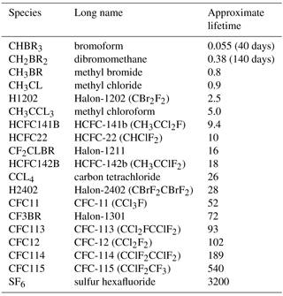
The stratospheric chemistry scheme explicitly treats the oxidation and photolysis of 21 halogenated compounds listed in Table 2 together with their approximate lifetimes. Heterogeneous reactions occur on four types of particles:
-
liquid binary sulfate (LBS);
-
supercooled ternary solution (STS);
-
nitric acid tri-hydrate (NAT); = and
-
water ice.
For details, see the Supplement of Kinnison et al. (2007).
The complete listing of the JAM002 species and reaction equations can be found in Supplement 1 (Tables S1–S23). In total, JAM002 contains 246 species and 734 reactions, including 142 photolysis reactions.
MOZ uses the same chemical preprocessor as CAM-Chem (Lamarque et al., 2012) and WACCM (Kinnison et al., 2007) to generate FORTRAN code, which contains the chemical solver for a specific chemical mechanism. In ECHAM-HAMMOZ, all reactions are treated with the semi-implicit (Euler backward integration) solver. This solver uses efficient sparse matrix techniques (LU decomposition and Newton–Raphson iteration) and is set up as follows: within the outer time step loop, up to 11 iterations are performed to achieve a solution within the prescribed relative accuracy. For ozone, NO, NO2, NO3, HNO3, HO2NO2, N2O5, OH, and HO2, a relative error of less than 10−4 is required and less than 10−3 for all other species. If convergence is not reached after 11 iterations, the time step is halved and the calculation is repeated. This may happen up to five times. If convergence is still not achieved, a warning message is written into the log file, and the calculation continues. A 3-day test simulation with detailed diagnostics on the solver behavior showed no cases in which the time step length had to be reduced, and convergence was always reached after two to six iterations. As expected, the largest number of iterations occurred under conditions of sunrise and sunset. The model is parallelized in a way that blocks of entire vertical columns on several adjacent longitudes are passed to the solver together, and the convergence threshold is evaluated for the entire block for efficiency reasons. This implies that changing the vector length of the parallelization will affect the results of the chemical calculations (within the error limits given above). More details on the MOZ chemical solver can be found in the Supplement of Kinnison et al. (2007).
The preprocessor code is available with the ECHAM-HAMMOZ model distribution. A simplified chemistry scheme for stratospheric applications (GEOMAR Atmospheric Mechanism; GAM) is also available and can easily be used in lieu of the extensive JAM002 mechanism (in preparation).
Table 1Primary volatile organic compounds and their oxidants in the JAM002 mechanism. BIGALKANE is a lumped species for all alkanes C4 and greater, BIGENE lumps all alkenes C4 and greater, and o-, m-, and p-xylene are lumped into one xylene species. CH4 is also oxidized by O(1D) and F, CH2O is also oxidized by O and HO2, DMS is also oxidized by BrO, and CH3Br and HCN are also oxidized by O(1D).
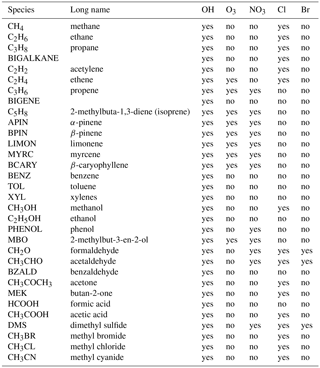
Table 2Halogenated compounds in JAM002 with relevance for stratospheric ozone chemistry and their approximate lifetimes in years (Miller et al., 1998; Liang et al., 2010; WMO, 2014; Harrison et al., 2016).
3.1 Emissions
All emissions in the ECHAM-HAMMOZ model are controlled via a single “emi_spec” file, which provides a simple and compact way to define all trace gas and aerosol emissions used in a model simulation and ensures proper documentation of the emissions used in a specific run. The emi_spec file consists of three sections: (1) definition of emission sectors and the source of emission information for this sector; (2) the species–sector matrix controlling which emission sectors are active for which species; and (3) an alias table that allows the mapping of species names from emission files to the names that are defined in the chemical mechanism. The emi_spec file that was used in the simulations of this paper is provided in Supplement 2.
In the sector definition, users can specify if emissions from that sector shall be read from the file or if an interactive parameterization (if available) shall be applied. In addition, it is possible to specify a single number to be used as a globally uniform emission mass flux. Furthermore, it can be decided to apply the emissions as a boundary flux condition to the lowest model level, to inject them at the model level near 50 m of altitude (smoke stack emissions), or to distribute them within a specific range of the atmosphere. For biomass burning emissions a special option is available to distribute them across the planetary boundary layer. Finally, the user can also select if emissions shall be interpolated in time or not and if the year of the date information in an emissions file shall be ignored in order to treat emissions as climatology. The simulations shown in this article were performed without time interpolation and using emissions for specific years.
The species–sector matrix has a single float number or a dash in each cell. The float number can be used to easily scale emissions from a particular sector for a particular species or to define emissions for compounds for which no emission data are available by scaling these emissions to those of other compounds (this requires an entry in the alias table). A dash indicates that no emissions for this compound are available in the given sector and is distinct from a zero, which would attempt to read or calculate emissions and then scale them to zero afterwards.
Emission files can be provided in any time resolution (minimum daily). Normally, all emissions files contain monthly data, except for fire emissions, which are provided in daily resolution in the standard configuration.
Table 3Emissions of trace gases and aerosols used in the standard configuration of ECHAM-HAMMOZ for the year 2008.
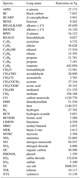
With JAM002 and either HAM-M7 or HAM-SALSA as an aerosol module, ECHAM-HAMMOZ has emissions for a total of 43 species that are emitted in 20 sectors. Table 3 lists all emissions for the year 2008.
In the standard configuration of ECHAM-HAMMOZ, the following emissions are calculated interactively:
-
VOC emissions from terrestrial vegetation (MEGAN; Guenther et al., 2012; implementation details in Henrot et al., 2017);
-
DMS emissions from the oceans (Kloster et al., 2006; Lana et al., 2011);
-
dust (Tegen et al., 2002; Stier et al., 2005);
-
sea salt (Guelle et al., 2001); and
-
volcanic sulfur (Dentener et al., 2006b).
Emissions from agriculture (AGR) and waste burning (AWB), forest fires (FFIRE) and grassland fires (GFIRE), aircraft (AIRC), domestic fuel use (DOM), energy generation, including fossil fuel extraction (ENE), industry (IND), ship traffic (SHP), solvent use (SLV), transportation (TRA), and waste management (WST) are taken from the Atmospheric Chemistry and Climate Model Intercomparison Project (ACCMIP; Lamarque et al., 2010). More specifically, as the simulations described here focus on the period after 2000, we make use of the Representative Concentration Pathway (RCP) 8.5 emissions (van Vuuren et al., 2011). The original files, which had a temporal resolution of 10 years, were interpolated to individual years and seasonal cycles were added (Granier et al., 2011). The netCDF emission data files are available from a WebDAV server at the Forschungszentrum Jülich (http://accmip-emis.iek.fz-juelich.de/) and contain detailed README and metadata information.
Ocean emissions of reactive VOCs were obtained from the POET project (Granier et al., 2005), and terrestrial DMS emissions are from Dentener et al. (2006b).
3.2 Lightning
As described in Rast et al. (2014), lightning NOx emissions are parameterized as a function of the average convective updraft velocity in a model column following Grewe et al. (2001). Flash frequency is calculated as
with , β=4.9, m s−1, and d0=1 m; d is the vertical cloud extent. Due to the coarse model resolution, a correction factor of 0.7 is applied to the result of this formula to yield a global flash frequency of 49 flashes per second for the year 2008, which is within the uncertainty of 44 ± 5 flashes per second observed from the Optical Transient Detector satellite instrument during 1995 to 2000 (Christian et al., 2003).
The fraction of cloud-to-ground flashes is calculated according to Price and Rind (1994) as
where dc denotes the cold cloud thickness, i.e., the vertical extent of the part of the cloud with temperatures below freezing. Following Price et al. (1997) the amount of NO generated per flash is given as 1×10¹⁷ , and average flash energies are assumed to be 6.7×10⁹ J for cloud-to-ground flashes; one-tenth of this is for intra- and inter-cloud flashes. With these factors applied, the global amount of NO generated from lightning in the year 2008 would be 5.05 Tg(N), which is well within the range of other estimates (e.g., Schumann and Huntrieser, 2007) and was recommended as a target value in earlier model intercomparison projects. As we found a significant influence of global lightning NOx on global tropospheric ozone and OH (see Sect. 6) with methane and methylchloroform lifetimes more in the range of the literature values at lower lightning NOx, we scaled the lightning emissions down. In the default configuration of the model, global lightning NOx emissions from the simulation described in this study for the year 2008 are 1.2 Tg(N). Within the model column, the NO from lightning is distributed according to the climatological vertical profiles of Pickering et al. (1998).
3.3 Lower boundary conditions for long-lived stratospheric species
Halogenated species, which are primarily decomposed in the stratosphere, are not emitted into the model, but instead a lower boundary condition is specified for these compounds. In addition to the species in Table 2 the model also specifies lower boundary conditions for N2O, CH4, and CO2. The latter can be turned off if the model is run with all carbon cycle components. The lower boundary conditions are provided as zonally averaged, monthly values from the Whole Atmosphere Chemistry Climate Model (WACCM) input for the simulations in the Chemistry–Climate Model Initiative (CCMI) initiative (see Sect. 2.3.2 in Tilmes et al., 2016). The organic halogen scenario (here, RCP8.5) is based on WMO (2011) and described in Eyring et al. (2013) and Morgenstern et al. (2017). Boundary conditions for N2O, CH4, and CO2 are taken from Meinshausen et al. (2011) as recommended by CCMI. As described in Tilmes et al. (2016), the boundary conditions used in ECHAM-HAMMOZ include a latitudinal gradient based on aircraft measurements from the HIAPER (High-Performance Instrumented Airborne Platform for Environmental Research) Pole-to-Pole Observations (HIPPO) campaigns (Wofsy et al., 2011).
The lower boundary condition for methane uses a relaxation to the climatological values with an e-folding time of 3 days in order to preserve regional methane emission patterns while at the same time preventing a drift of methane concentrations due to possibly unbalanced sources and sinks (see Rast et al., 2014).
3.4 Photolysis
As described in the Supplement of Kinnison et al. (2007), photolysis frequencies are calculated as a product of the prescribed extra-atmospheric solar flux, the atmospheric transmission function (dependent on model-calculated ozone and O2), the molecular absorption cross section, and the quantum yield of the specific reaction channel. There are 34 channels in the wavelength regime from 120 to 200 nm and 122 channels between 200 and 750 nm. At wavelengths less than 200 nm, the transmission function is computed explicitly, and absorption cross sections and quantum yields are prescribed, except for O2 and NO, for which detailed parameterizations are used (see the Supplement of Kinnison et al., 2007). Beyond 200 nm, the transmission function is calculated from a lookup table as a function of altitude, column ozone, surface albedo, and zenith angle. The maximum zenith angle for which photolysis frequencies are calculated is 97∘. The temperature and pressure dependence of absorption cross sections and quantum yields is also interpolated from lookup tables.
The UV albedo is parameterized according to Laepple et al. (2005) using satellite-derived albedo maps for snow and non-snow conditions based on the Moderate Resolution Imaging Spectroradiometer (MODIS) instrument. The threshold for switching from non-snow to snow values is a snow depth of 1 cm calculated by ECHAM. Sea ice albedo is prescribed as 0.78 in the Northern Hemisphere and 0.89 in the Southern Hemisphere. The albedo over ice-free oceans is set to 0.07. The influence of clouds is parameterized according to Brasseur et al. (1998) through the computation of an effective albedo and modification of the atmospheric transmission function. Both effects are combined into a single factor that varies by model level.
3.5 Dry deposition
Deposition of trace gases and aerosols on the Earth's surface is parameterized according to the resistance model of Wesely (1989) using a big-leaf approach for vegetated surfaces (Ganzeveld and Lelieveld, 1995). The ECHAM-HAMMOZ dry deposition scheme distinguishes between vegetated land surfaces, bare soils, water, and snow or ice and uses the corresponding surface types from the JSBACH land model (see Sect. 2.1).
As described in Stier et al. (2005), the leaf area index is taken from an NDVI (normalized differential vegetation index) climatology (Gutman et al., 1995) and the Olson (1992) ecosystem database. Canopy height, roughness length, and forest fraction are from a climatology. Soil pH is specified for 11 different soil types. Technically, these parameters can also be obtained online from the JSBACH land surface model. This has been tested in Stanelle et al. (2014), but this coupling has not been used in the simulations described in this study.
Surface resistances are explicitly specified for H2SO4, HNO3, NO, NO2, O3, and SO2. Those of other species are calculated relative to O3 and SO2 following Wesely (1989). A dynamic coupling of stomatal resistance with JSBACH has not been implemented. Henry coefficients and reactivity factors have been defined for 137 species (see Table S24 in Supplement 1). All of these species can be deposited; however, for most of them the deposition rates will be very small due to low Henry values or low reactivities. Where available, Henry coefficients were taken from the literature, and in other cases we assumed that molecules with similar structures have Henry values on the same order of magnitude. In particular, OOH groups were considered similar to OH groups in terms of their impact on Henry constants. Organic peroxides (ROOH) are assumed to have a surface reactivity f0 of 1. Other organic molecules with oxygen were assigned with f0=0.1. Note that while HO2 can undergo dry deposition (H=690 M atm−1), we did not define Henry values and surface reactivities for organic peroxy radicals, although some of these (notably from higher oxidation states) might well be soluble and could therefore be efficiently removed by dry deposition.
3.6 Wet deposition and scavenging
The ECHAM-HAMMOZ wet deposition scheme is based on Croft et al. (2009) for below-cloud scavenging by rain and snow and Croft et al. (2010) for in-cloud (nucleation and impaction) scavenging. The in-cloud scavenging scheme treats nucleation and impact scavenging in stratiform and convective clouds and distinguishes between warm, cold, and mixed-phase clouds. For aerosols, scavenging also takes place below clouds in rain and snow. For gases, the gas-phase liquid-phase equilibrium is calculated based on Henry's law (see Table S2), and no below-cloud scavenging takes place except for HNO3 and H2SO4.
The simulations described in this article are based on the ECHAM-HAMMOZ model version and input datasets as released in February 2017. The base run is a 10-year simulation from October 2002 through December 2012. The simulation started with initial conditions for October 2002 taken from the Monitoring Atmospheric Composition and Climate (MACC) reanalysis described by Inness et al. (2013). The first 3 months are used as spin-up time and are not used in the analysis of results. Note that the stratosphere takes about 4 years to reach a dynamically stable state (see Fig. S3.1 in the Supplement 3).
The model resolution is in longitude and latitude (spectral triangular truncation T63), with 47 vertical levels from the surface to 0.01 hPa (full level pressure). The corresponding model time step is 7.5 min. Sea surface temperatures and sea ice coverage are prescribed for each year of simulation, following the Coupled Model Intercomparison Project Phase 5 (CMIP5) AMIP simulation protocol (Giorgetta et al., 2012). In addition, temperature, vorticity, divergence, and surface pressure from 6-hourly output of the European Centre for Medium-Range Weather Forecasts (ECMWF) ERA-Interim reanalysis (Dee et al., 2011) were used to specify the dynamics of “real weather” in nudging mode (Kaas et al., 2000). The simulation includes full interaction between aerosols and gas-phase chemistry, full feedback of aerosols and trace gases on the radiation, and feedback of chemically produced water in the stratosphere onto the climate model. All simulations performed for this study use the HAM-M7 aerosol scheme for aerosol formation and microphysical processes.
Some of the analyses presented below discuss the 10-year core period of the simulation, while the more detailed comparisons with observations focus on the year 2008. This year was chosen as a reference year by the HAMMOZ consortium because of data availability and because it has been used in several other studies and in the Copernicus Atmospheric Monitoring Service validation activities (Eskes et al., 2015). The year 2008 began with La Niña conditions and turned neutral by June. The global average temperature was 0.49 K above the 20th century mean (NOAA, 2008), but looking back from 2012, the end year of our simulation, it is not among the 10 warmest years on record (NOAA, 2012). In terms of Antarctic ozone depletion, 2008 was relatively close to the 1979–2007 average (WMO, 2008).
Table 4Summary of simulations performed for the analysis of global trace gas budgets in this article.
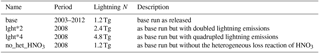
As described above, the released model version has very low lightning NO emissions, and the parameterization of the heterogeneous reaction of HNO3 neglects the potential of reevaporation of aerosol nitrate to gaseous HNO3 (Stadtler et al., 2017), which has an impact on the total amount of deposited nitrogen and also affects the budgets of ozone and nitrogen oxides as shown below. In order to investigate the impacts of these two factors we performed a small series of sensitivity simulations for the year 2008 based on restart files of the reference run. Table 4 briefly describes these simulations. Two of the simulations double and quadruple the amount of lightning emissions, respectively, so that they are more in line with current estimates ranging from 2 to 8 Tg(N) yr−1 (Schumann and Huntrieser, 2007). The other simulation deactivates the heterogeneous reaction of HNO3 on sea salt and dust and is otherwise identical to the base run.
5.1 Total column ozone and stratospheric processes
We begin our model evaluation with a discussion of seasonal total column ozone (TCO) distributions in comparison with retrievals from the Infrared Atmospheric Sounding Interferometer (IASI), onboard the sun-synchronous polar-orbiting MetOp platforms, and from the Ozone Monitoring Instrument (OMI) onboard the Aura satellite (Levelt et al., 2006). Furthermore, the 10-year evolution of TCO has been compared to the The Modern-Era Retrospective Analysis for Research and Applications version 2 (MERRA-2), for which a large variety of satellite retrievals were assimilated (Gelaro et al., 2017).
IASI is a high-resolution Fourier transform spectrometer designed to measure the outgoing thermal infrared radiation from the Earth's surface and the atmosphere in a nadir-viewing geometry (Clerbaux et al., 2009). The first IASI instrument was launched in 2006 on the MetOp-A platform and it is still operating. A second instrument onboard MetOp-B was launched in 2012. IASI observations – a set of four simultaneous footprints of 12 km at nadir – are performed every 50 km along the track of the satellite at nadir and across-track over a swath width of 2200 km. IASI crosses the Equator at around 09:30 and 21:30 mean local solar time, achieving near global coverage twice a day. The vertical abundance and distribution of O3 and CO are retrieved in near real time from individual IASI measurements with the Fast Optimal Retrievals on Layers for IASI (FORLI) algorithm (fully described in Hurtmans et al., 2012). IASI measurements are filtered out based on the cloud coverage and several quality flags to ensure stable and consistent products. The estimated errors on the retrieved total columns are mainly latitude dependent. For O3, such errors are usually below 3 %, but slightly larger (∼ 7.5 %) when the signal is particularly weak over the Antarctic ozone hole or due to strong water vapor influence at tropical latitudes (Hurtmans et al., 2012). The error on the retrieved CO total columns is generally below 10–15 % at middle and tropical latitudes, but increases up to 20–25 % in polar regions (George et al., 2015). All details as to the retrieval methodology, characterization of the retrieved products, and validation against a large suite of independent ground-based, airborne, and satellite measurements can be found in previous studies (Hurtmans et al., 2012; George et al., 2015; Boynard et al., 2016, 2018; Wespes et al., 2016, 2017).
For a meaningful model-to-satellite comparison, daily average ECHAM-HAMMOZ vertical profiles of O3 and CO have been smoothed with the IASI averaging kernels (A) to account for the vertical sensitivity of the instrument to the species. The model profiles were firstly vertically interpolated onto the IASI retrieval levels. Then the smoothing of the model profiles (Xmodel) to the lower vertical resolution of the IASI measurements was performed following the formalism of Rodgers (2000):
where Xsmoothed is the smoothed model profile and Xa is the a priori profile. As numerous IASI observations are usually available for a given day and grid cell, the total columns calculated from the smoothed model profiles were averaged to generate one daily mean value.
Figure 1 compares seasonal mean total ozone columns of the year 2008 from IASI with the ECHAM-HAMMOZ outputs smoothed by the IASI sensitivity functions. The model generally captures the highs and lows that are observed by the satellite as well as the changes in these patterns throughout the seasons. It shows a tendency to underestimate the total ozone column in middle to high northern latitudes (< 10 %; i.e., 5–30 DU) and over the Antarctic (< 15 %; i.e., 10–40 DU) in all seasons, while it overestimates over the tropical regions (< 5 %; i.e., 10 DU) and the southern midlatitudes (∼ 10 %; i.e., 25 DU). These IASI–model discrepancies are generally larger than the errors on the retrieved TCO (see above) and the IASI-UV instrument biases recently reported in the validation experiment of Boynard et al. (2018). These authors report errors that are generally lower than 5 %, with a global bias of 0.1–2 %.

Figure 1(a, b) Comparison of seasonal mean total column ozone (in DU) from ECHAM-HAMMOZ with data from the IASI instrument. Data and model results are from 2008. IASI data were interpolated onto the model grid and averaging kernels were applied to the model data. (c) TCO relative differences (in %) between ECHAM-HAMMOZ and IASI.

Figure 2Comparison of the seasonal cycle of zonal mean total column ozone (in DU) between ECHAM-HAMMOZ (a) and Aura OMI (b). Data and model are for the year 2008. Aura OMI data were interpolated to model grid.
OMI is an ultraviolet visible nadir-viewing solar backscatter spectrometer. We use the level 3 data product, which is globally gridded to 1∘ latitude by 1∘ longitude. The Aura OMI data span the temporal range from 2004 to present. Daily OMI data were interpolated to the model resolution and compared to the model results as latitude–time series plots in Fig. 2. Unlike the comparison of the model to IASI observations in Fig. 1, this analysis has not applied the OMI averaging kernel to the model results, and therefore one needs to be careful in overstating any biases between the model and the observations. A discussion of biases among satellite TCO products is beyond the scope of this paper.
The purpose of Fig. 2 is to document that the model nicely represents the overall zonal mean latitude versus time structure compared to OMI. Both the Northern and Southern Hemisphere spring maxima are consistent with OMI along with the tropical minimum in TCO around 260 DU. The Southern Hemisphere ozone hole is also well represented, suggesting that the heterogeneous chemistry defining the Antarctic ozone hole is adequately formulated in the model (see Solomon, 1999, and references within).
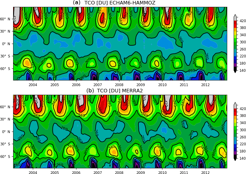
Figure 3The 10-year latitude–time variations in the total ozone column in ECHAM-HAMMOZ (a) and in the MERRA-2 reanalysis (b). A difference plot can be found in the Supplement.
Figure 3 shows a comparison between the latitude–time variations in TCO during the 10 years of our ECHAM-HAMMOZ reference simulations with TCO from the MERRA-2 reanalysis (Gelaro et al., 2017). Generally, the differences in TCO remain below 6 % (see also Fig. S3.1 in the Supplement), which is similar to the accuracy estimate of Wargan et al. (2017) for the MERRA-2 stratospheric ozone field. The interannual variabilities of the springtime ozone maximum in the Northern Hemisphere and the Antarctic minimum are well captured. The model slightly underestimates TCO in the tropics, and it has a tendency to underestimate the Southern Hemisphere midlatitude maxima during austral spring. Closer inspection of the differences (Fig. S3.1) reveals larger biases during the first 4 years of the simulation. These can be attributed to the initial conditions, which, although suitable for October 2002, i.e., the beginning of our simulation, were taken from a different model and might therefore reflect a somewhat different stratospheric state than what ECHAM-HAMMOZ would have simulated with a longer spin-up period. A decay time of 4 years for TCO disturbances is quite reasonable and indicates a reasonable representation of the stratospheric age of air, which has not been explicitly evaluated for this model.
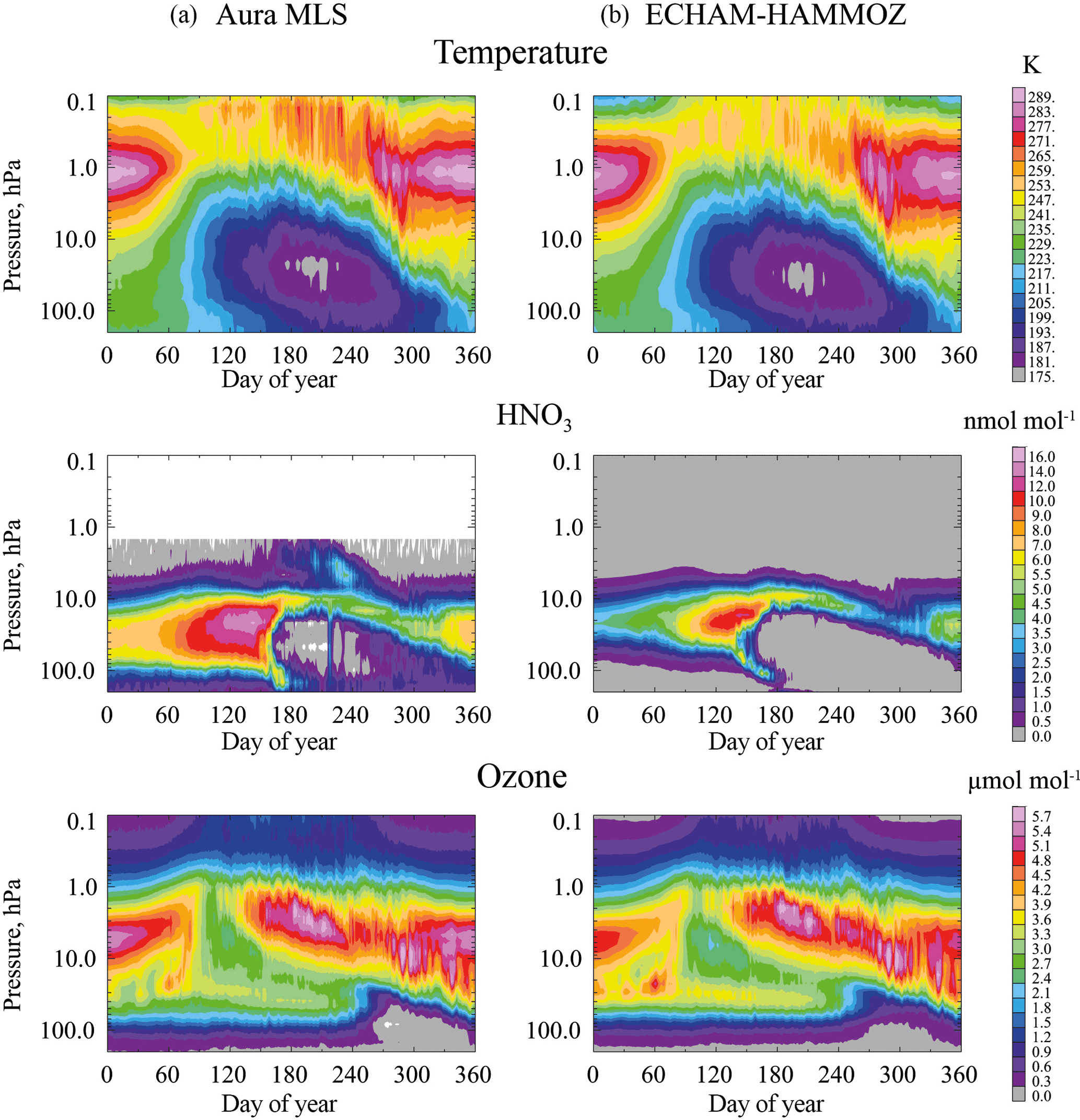
Figure 4Comparison of temperature, HNO3, and O3 between Aura MLS observations (a) and ECHAM-HAMMOZ (b). Data and model are for the year 2008.
Figure 4 further explores the representation of the Antarctic region by showing a time-dependent vertical cross section of key constituents at 81∘ S. In this figure, model results of temperature, nitric acid (HNO3), and ozone are compared to daily binned (4.5∘ latitude × 10∘ longitude) data from version 4 of the Microwave Limb Sounder (MLS) instrument onboard the Aura satellite. Details of the accuracy and precision of the MLS observations are discussed in Livesey et al. (2016). Since polar heterogeneous chemistry is very temperature sensitive (e.g., Solomon et al., 2015) it is important to have an accurate representation of temperature when comparing model results to observational data for a given year. Even in a nudged simulation, temperature biases in the lower stratosphere can amount to a few degrees (Krefting, 2017). Figure 4, row 1 shows excellent agreement between the retrieved MLS temperatures and those used in ECHAM-HAMMOZ, giving confidence that there are no model temperature biases that could impact the heterogeneous chemistry derived in the model.
Another important constituent to show is HNO3. Here, the HNO3 gas-phase abundance is affected by the formation of NAT PSC particles, which can settle out of the stratosphere and cause irreversible denitrification. Figure 4, row 2 shows that the model adequately represents the HNO3 abundance and the process that controls the loss of total inorganic nitrogen in the model atmosphere. If anything, the model over-denitrifies by 0.5 nmol mol−1. This result is consistent with use of the current ECHAM-HAMMOZ heterogeneous chemistry module (Kinnison et al., 2007) in other model frameworks, e.g., the Whole Atmosphere Chemistry Climate Model version 3 (see evaluation in SPARC, 2010). The model does show a low bias in HNO3 between January and May in the pressure range of 80–10 hPa. This low bias is not due to the effect of denitrification, since this process starts in June. The model does not include a representation of lower mesospheric and stratospheric particle production of NOx. However, the descent of NOx from these processes and the eventual formation of HNO3 would not affect the lower stratosphere until later in the austral winter. The model does include the heterogeneous conversion of N2O5 to HNO3 on sulfate aerosol (Austin et al., 1986). Future work to better understand this bias will need to focus on the tropical gas-phase net production of NOy and subsequent meridional transport to higher latitudes.
The ozone evolution is shown in Fig. 4, row 3. The overall representation of ozone from the lower mesosphere to the lower stratosphere is captured by the model. However, in the lower stratosphere spring, the model is biased high by approximately +0.5 µmol mol−1. This high ozone bias translates to the model having too much TCO in the Antarctic spring period, which is consistent with Fig. 2.
5.2 Tropospheric ozone
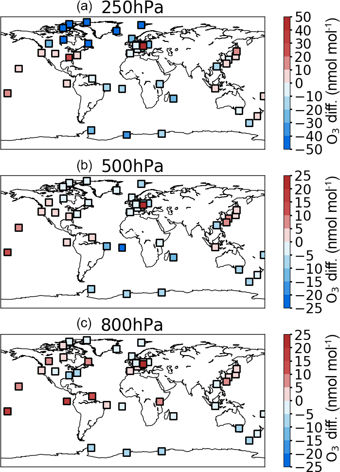
Figure 5Annual mean bias of ECHAM-HAMMOZ with respect to ozonesonde data from Tilmes et al. (2012) at 250 hPa (a), 500 hPa (b), and 800 hPa (c). At 250 hPa the relative error is shown for better visibility. Figure layout and scales are comparable to Lamarque et al. (2012).
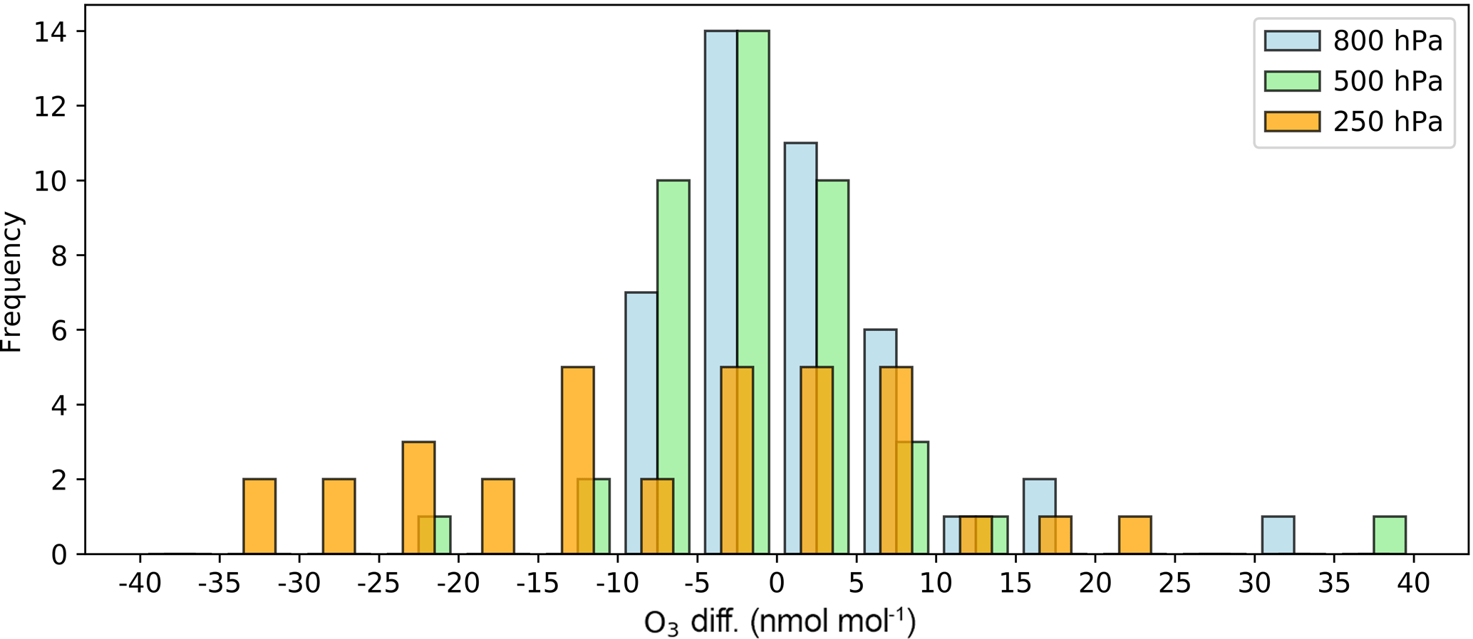
Figure 6Frequency distributions of the ozone bias (in nmol nmol−1) at the 42 stations from Tilmes et al. (2012). Note: high northern latitude stations with biases larger than ±40 nmol nmol−1 at 250 hPa are not shown.
Figure 5 shows the year 2008 annual mean bias of ozone in comparison to the ozonesonde climatology of Tilmes et al. (2012) at three different pressure levels. For ease of comparison, we have chosen a similar layout and scale as Lamarque et al. (2012). At 250 hPa, the biases are generally between −35 and +35 nmol nmol−1 with the exception of high northern latitude stations, where the bias is as low as −114 nmol nmol−1 (Eureka and Resolute, Canada) and Prague, Czech Republic, where the bias is +66 nmol nmol−1. The model overestimate at high northern latitudes is qualitatively similar to CAM-Chem (Lamarque et al., 2012). We concur with Lamarque et al. (2012) that the reason is likely associated with a mismatch between the model tropopause and the real tropopause in this region. Due to the very steep gradients of ozone around the tropopause, even small vertical displacements can lead to large discrepancies in simulated ozone values if the comparison is made on pressure levels. Future work should probably consider evaluating models with ozonesonde data relative to the tropopause. For comparison, Fig. S3.2 in the Supplement presents plots similar to Fig. 5, but for the simulation lght*4.
In contrast to CAM-Chem, the Northern Hemisphere midlatitude biases in ECHAM-HAMMOZ are more or less equally distributed. One may discern a tendency of the model to overestimate ozone at 250 hPa around the Pacific, whereas there appears to be underestimation around the Atlantic.
At 500 hPa, the pattern of the ECHAM-HAMMOZ biases is similar to that at the 250 hPa level, but the values are generally smaller. Only 6 stations out of 42 have biases with absolute values larger than 10 nmol nmol−1, and 5 of these 6 stations are located in the tropics. Ascension, Natal, and Reunion exhibit large low biases, whereas high biases are found at Hilo, Hawaii, and Samoa. At 800 hPa the biases are somewhat shifted to more positive values so that no site has a low bias of more than 10 nmol nmol−1, and four stations show a high bias greater 10 nmol nmol−1. Averaged over all 42 sites, the mean biases at 250, 500, and 800 hPa are −17.8, −1.5, and +1.6 nmol nmol−1, respectively. If we exclude the high-latitude Northern Hemisphere stations, the bias at 250 hPa is reduced to −3.6 nmol nmol−1. Figure 6 shows frequency distributions of the model biases at the three pressure levels.
The seasonal cycle of tropospheric ozone is evaluated with the help of Taylor plots in Fig. 7. Similar to Lamarque et al. (2012) we show regional averages at the three model levels of Fig. 5. However, we retain the original region definitions and color codings of Tilmes et al. (2012). Taylor plots with individual stations and also for the sensitivity run lght*4 can be found in Fig. S3.3. For seven out of nine regions, the correlation between the observed and simulated seasonal cycle is positive so that the symbols appear in Figure 7. Exceptions are Canada and the tropics. The normalized root mean square error (concentric gray circles around a standard deviation ratio of 1 and a correlation of 1) is generally below 0.8. Exceptions are the eastern Northern Hemisphere polar stations at 250 hPa, the Southern Hemisphere polar stations at 500 and 800 hPa, and the Southern Hemisphere midlatitude stations at 800 hPa. At 250 hPa the correlation is better than 0.7 over most regions, and exceptionally good results are obtained over the Northern Hemisphere western polar region. The correlation slightly worsens at 500 and 800 hPa, but generally remains better than 0.6. Across all 42 sites, the average correlation coefficients at 250, 500, and 800 hPa are 0.59, 0.59, and 0.68, respectively. If we leave out the tropics, which have the worst correlation, they increase to 0.68, 0.68, and 0.73, respectively.
Hence, as a summary, we can state that tropospheric ozone in the base run is very well simulated with two exceptions: (1) there is a severe underestimate at high northern latitude sites at 250 hPa, and (2) the (small) seasonal cycle over the tropics is not well captured.
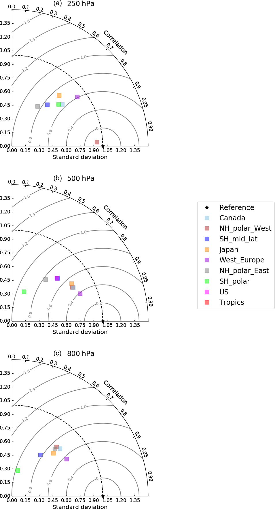
Figure 7Taylor plots of regional averaged ozonesondes at 250 hPa (a), 500 hPa (b), and 800 hPa (c). Ozonesonde data and region definitions are from Tilmes et al. (2012). Where a region is not shown in a panel, the respective data point is outside the axis range.
5.3 Surface ozone
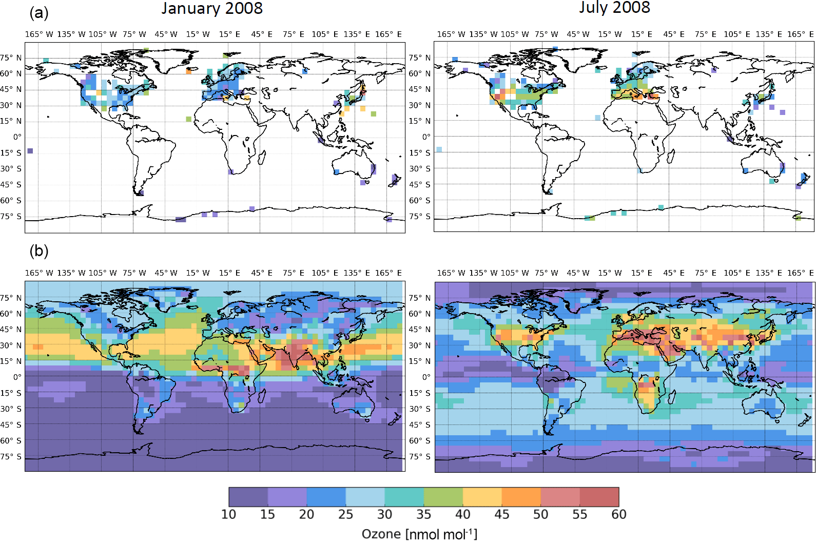
Figure 8Comparison of gridded rural surface ozone observations from the TOAR database (Schultz et al., 2017) (a) with ECHAM-HAMMOZ output (b) for January and July 2008. The model results have been regridded to 5∘ × 5∘ to match the resolution of the observations.
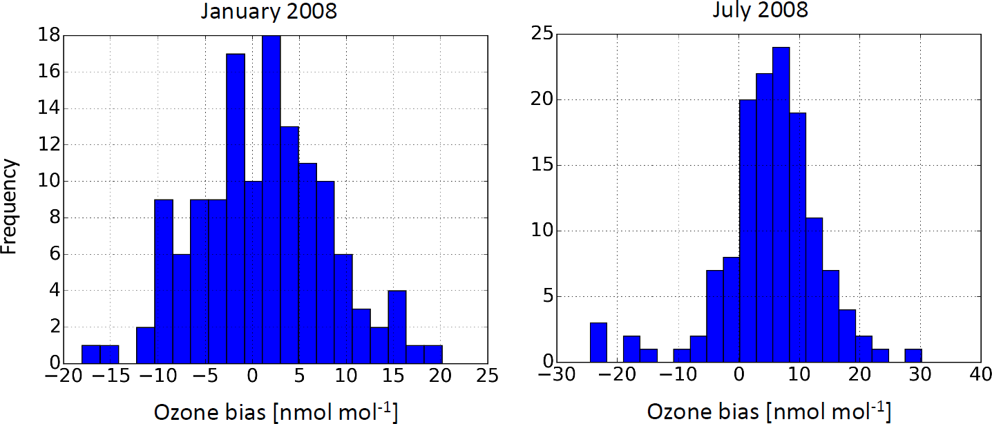
Figure 9Monthly mean bias of surface ozone mixing ratios in January and July 2008 for all 5∘ × 5∘ grid boxes for which the TOAR database contains data in 2008.
For the evaluation of ECHAM-HAMMOZ with surface ozone observations, we make use of the recently published database from the Tropospheric Ozone Assessment Report (TOAR). As described in Schultz et al. (2017), this database contains hourly data from more than 9000 scientific and air quality monitoring stations worldwide, and it has a globally consistent classification scheme to distinguish urban from rural locations. The classification scheme is based on threshold combinations of global satellite data products of nighttime light intensity, population density, and OMI NO2 columns. For details see Schultz et al. (2017).
Figure 8 shows gridded maps of TOAR data at rural stations (top row) in comparison with ECHAM-HAMMOZ base run output regridded to the same resolution of 5∘ × 5∘ for January and July 2008. Figure 9 displays the bias between the model and observations. The first thing that becomes apparent in Fig. 8 is the evident geographical bias of the observation database. About three-quarters of the grid boxes with measurements by rural stations are located either in Europe or North America, and the rest is scattered across the world. The problem of insufficient observational coverage of reactive gas measurements is widely known, and the community has yet to develop a sound strategy to deal with it.
Where measurements exist, the model generally shows good agreement with the observations in both January and July. During the boreal summer, ozone over the eastern US and the North Sea–Baltic Sea region is somewhat overestimated. Closer inspection reveals differences of up to −25 and +30 nmol nmol−1 in individual grid boxes, for example over the Mediterranean or in Nebraska, US. However, altogether the model yields excellent agreement with mean bias of 1.13 nmol mol−1 in January and 5.28 nmol mol−1 in July. Additional information, also concerning the sensitivity experiments lght*2 and lght*4, can be found in Figs. S3.4 and S3.5.
5.4 Total column CO
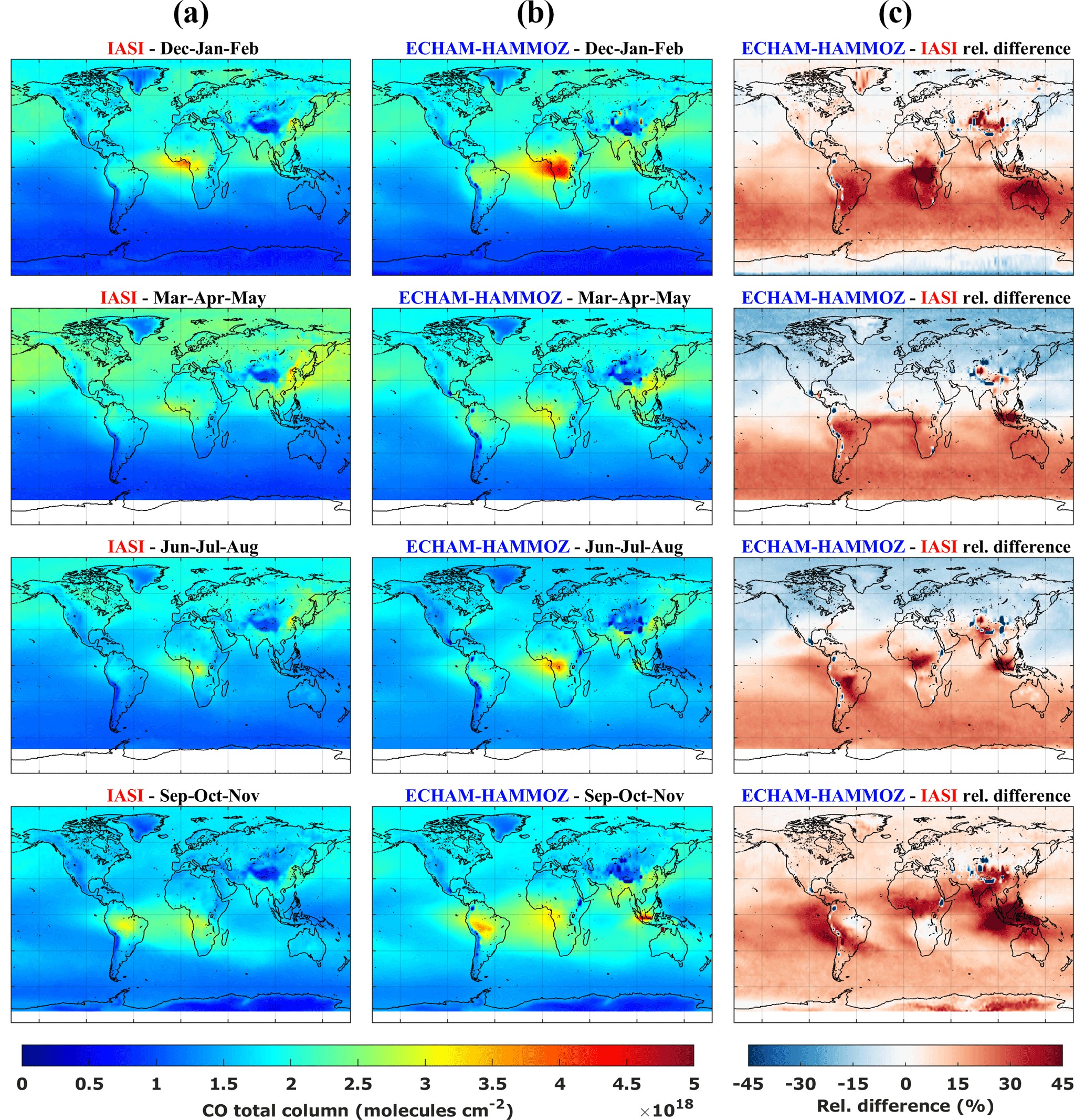
Figure 10(a, b) Comparison of seasonal mean total column CO (in 1018 cm−2) by ECHAM-HAMMOZ with data from the IASI instrument. Data and model results are from 2008. IASI data were interpolated onto the model grid and averaging kernels were applied to the model data. (c) CO total column relative differences (in %) between ECHAM-HAMMOZ and IASI.
Figure 10 shows seasonal mean total column CO from IASI in comparison with ECHAM-HAMMOZ smoothed by the IASI averaging kernels. The model reproduces the seasonal variations with the main features of the retrieval, but also shows a couple of differences.
-
The model tends to underestimate CO by about 15 % in the Northern Hemisphere, especially during spring and summer. Apparently, ECHAM-HAMMOZ loses CO too quickly during these seasons because of relatively high OH levels (see Sect. 6). Inaccurate emissions (see Sect. 5.5) and transport from polluted regions likely also contribute to the differences.
-
In the Southern Hemisphere a positive bias of 15–40 % is found, likely coming from an overestimation of the fire emissions in ACCMIP. The positive bias is particularly pronounced over Indonesia, central Africa, and Amazonia.
5.5 Surface CO
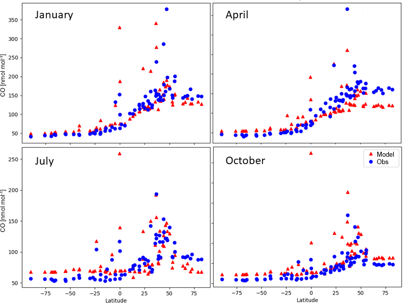
Figure 11Comparison of monthly mean surface CO measurements from GAW with ECHAM-HAMMOZ base run results for January, April, July, and October 2008. Each symbol represents data from one measurement location.
Figure 11 displays the latitudinal gradients of surface CO concentrations from the World Meteorological Organisation Global Atmosphere Watch (GAW) network (see Schultz et al., 2015) in comparison with ECHAM-HAMMOZ base run results for the year 2008. In general, the model captures the latitudinal variations of CO well throughout the year. However, in higher northern latitudes the simulated CO is underestimated by up to 40 nmol nmol−1 (33 %) in April and to a lesser degree also in January. The reasons for such model–observation discrepancies have been discussed in Stein et al. (2014) and are likely related to inaccurate emissions data in combination with excessive dry deposition of CO. The tendency of ECHAM-HAMMOZ to generate too much OH (see Sect. 6) could also play a role here. The model also overestimates CO in the Southern Hemisphere. This bias is largest during austral winter. The reasons for this bias are unclear at present, but could be related to excessive emissions from biomass burning (see Sect. 5.4). A similar pattern of difference was seen across the suite of ACCMIP models, as described in Naik et al. (2013).
6.1 Ozone and OH
Stevenson et al. (2006)Young et al. (2013)Naik et al. (2013)Lamarque et al. (2012)Jöckel et al. (2016)Table 5Global tropospheric ozone budgets and tropospheric methane lifetimes of the four ECHAM-HAMMOZ simulations described in Table 4. An ozone threshold of 150 nmol mol−1 is used to denote the tropopause. For comparison, multi-model mean values from Stevenson et al. (2006), Young et al. (2013), and Naik et al. (2013) and the “GEOS5” budget terms from Lamarque et al. (2012) are also included.
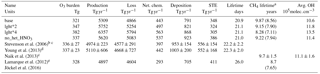
a Computed as whole atmosphere burden of CH4 over tropospheric loss of CH4 as in Naik et al. (2013). Values in parentheses were computed according to Jöckel et al. (2016) as tropospheric CH4 burden over tropospheric CH4 loss. b Values from selected models with relatively low O3 bias and CH4 lifetime close to the multi-model mean c year 2000 results.d Burden from 15 ACCMIP models, budget terms from 6 models. e Tropopause threshold at O3<100 nmol mol−1.
The global budgets of ozone and the tropospheric methane lifetime of the ECHAM-HAMMOZ base run are in the range of estimates from other recent models and model intercomparison studies (Table 5). The base run ozone burden is slightly lower than the averages of the multi-model studies. Production and loss terms are above the average plus 1 standard deviation of the selected models in Stevenson et al. (2006), but well in the range of models reported by Young et al. (2013). Since the HAMMOZ chemical mechanism resembles the CAM-Chem mechanism to a substantial degree, one might expect a better agreement with Lamarque et al. (2012), who report substantially lower values. However, Lamarque et al. (2012) used an ozone threshold of 100 nmol mol−1 for the tropopause definition, whereas all other studies in Table 5 used a threshold of 150 nmol mol−1. If we evaluate the base run ozone budget with a 100 nmol mol−1 threshold, we obtain a burden of 292 Tg and production and loss rates of 5192 and 4807 Tg yr−1, respectively.
The above-average ozone production and loss rates are most likely due to the more detailed VOC mechanism in ECHAM-HAMMOZ. Stevenson et al. (2006) noted that earlier model simulations with fewer primary VOC species tended to yield lower production and loss rates. Considering that our base run has very low lightning NOx emissions (at the low end of the models described in Young et al., 2013), it is somewhat surprising that our ozone chemistry is so active. The ozone lifetime is slightly shorter than the multi-model averages of Stevenson et al. (2006) and Young et al. (2013), but well within the range of these studies. Yet, the ozone lifetime of ECHAM-HAMMOZ is substantially shorter than the result reported by Lamarque et al. (2012) (19.2 days versus 26 days if we use their tropopause threshold of O3<100 nmol mol−1). As noted by Young et al. (2013): “Despite general agreement on how the drivers impact global-scale shifts in tropospheric ozone, magnitudes of the regional changes and the overall ozone budget vary considerably between different models.”
Figure 12 demonstrates that the tropospheric ozone budget of ECHAM-HAMMOZ remains rather stable over the 10 years of the reference simulation, although some effect from the spin-up can still be seen during the first half of the year 2003. The chemical production and loss terms peak in the boreal summer due to the greater impact of NOx and VOC emissions from the Northern Hemisphere land masses. We suggest that it might be illustrative to compare the seasonal cycles of individual ozone budget terms from different models in future studies to better understand the reported differences in global annual ozone budgets.
In ECHAM-HAMMOZ the tropical upper troposphere appears to play a prominent role for the global tropospheric trace gas budgets as evidenced by our lightning NOx sensitivity simulations. Table 6 lists the percent changes in the ozone budget terms when we double or quadruple the lightning NOx emissions. The tropics are the region with the highest frequency of thunderstorms and the highest flash density (Boccippio et al., 2000), and we do find the largest changes in the ozone budget in this region. For example, the chemical production of ozone increases by 33 % if we increase the lightning NOx emissions to 4.8 Tg(N) yr−1, a value close to the mean or median lightning NOx emissions of the models described in Young et al. (2013). The global increase in the ozone production is 1047 Tg yr−1 (Table 5), and the increase in the tropics constitutes 80 % of this change. The Northern Hemisphere is least affected by the increased lightning NOx source due to the much larger surface and aircraft emissions in this region. This is also reflected in the evaluation of the model runs with surface ozone observations (see Sect. 5.3): in spite of the large changes in the global budget terms and the substantial increase in the global burden, the mean bias in comparison with the gridded TOAR dataset of rural stations increases only moderately from 5.3 to 6.9 nmol mol−1. The density of stations in the Northern Hemisphere is much greater than elsewhere so that the larger changes in surface ozone in the tropics and Southern Hemisphere (see Fig. S3.3) are not accounted for in the bias calculation (Fig. S3.4).
The tropospheric average OH concentration and methane lifetime of our base run are close to the multi-model average diagnosed by Naik et al. (2013). If we increase lightning NOx emissions, OH increases and the CH4 lifetime decreases as expected. With 4.8 Tg(N) yr−1 as a global lightning source, the CH4 lifetime is 8.28 years, which is more than 2 standard deviations below the observational constraints from Prinn et al. (2005) and Prather et al. (2012). However, our CH4 lifetime appears rather consistent with the lifetime of Jöckel et al. (2016), who use a different method for the calculation (see footnote a of Table 5). Their year 2008 lifetime of 7.65 years falls between our lght*2 and lght*4 simulations if we apply the same method as Jöckel et al. (2016). Given that their lightning NOx emissions were about 4 Tg(N) yr−1 during this period, the agreement is remarkable. As a consequence we note that chemistry models that use the dynamical core and physics of ECHAM have a tendency to be too reactive and generate too much OH. This has already been an issue in earlier ECHAM-HAMMOZ model versions (e.g., Rast et al., 2014). Indeed, Baumgaertner et al. (2016) have shown that the dynamical core can have a large impact on the global CH4 lifetime. If we put this information in context with the analysis of regional ozone budget changes due to lightning NOx emission changes, we hypothesize that there is some issue with the dynamics or physics of ECHAM in the tropical troposphere that impacts its ability to reproduce the global budgets of reactive trace gases. A further hint in this direction is given by Stevens et al. (2013), who pointed out that both ECHAM5 (which forms the basis of the EMAC model reported by Jöckel et al., 2016) and ECHAM6 (the basis of ECHAM-HAMMOZ as described here) have a tropical precipitation bias of up to 5 mm day−1. Figure 13 shows the difference between a decadal ECHAM6.3 simulation (i.e., the ECHAM-HAMMOZ model without the chemistry and aerosol schemes) versus the ERA-Interim reanalysis (Dee et al., 2011), which confirms the statement of Stevens et al. (2013). In addition, the amounts of cloud liquid water and cloud ice are underestimated in the tropics (Lohmann and Neubauer, 2018), pointing to problems either with the parameterization of convection or detrained condensate with implications for the wet scavenging of trace gases and aerosol particles. A more detailed investigation of this issue is beyond the scope of this paper.
Table 6Percent changes in ozone budget terms in the Northern Hemisphere, the Southern Hemisphere, and the tropics of the simulations lght*2 and lght*4 versus the base run. The latitude boundary of the tropics was chosen at 20∘ N or S.
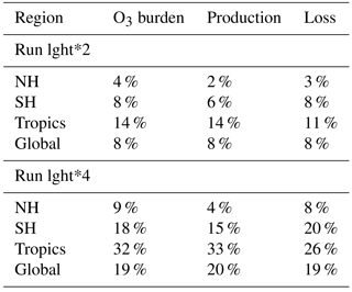
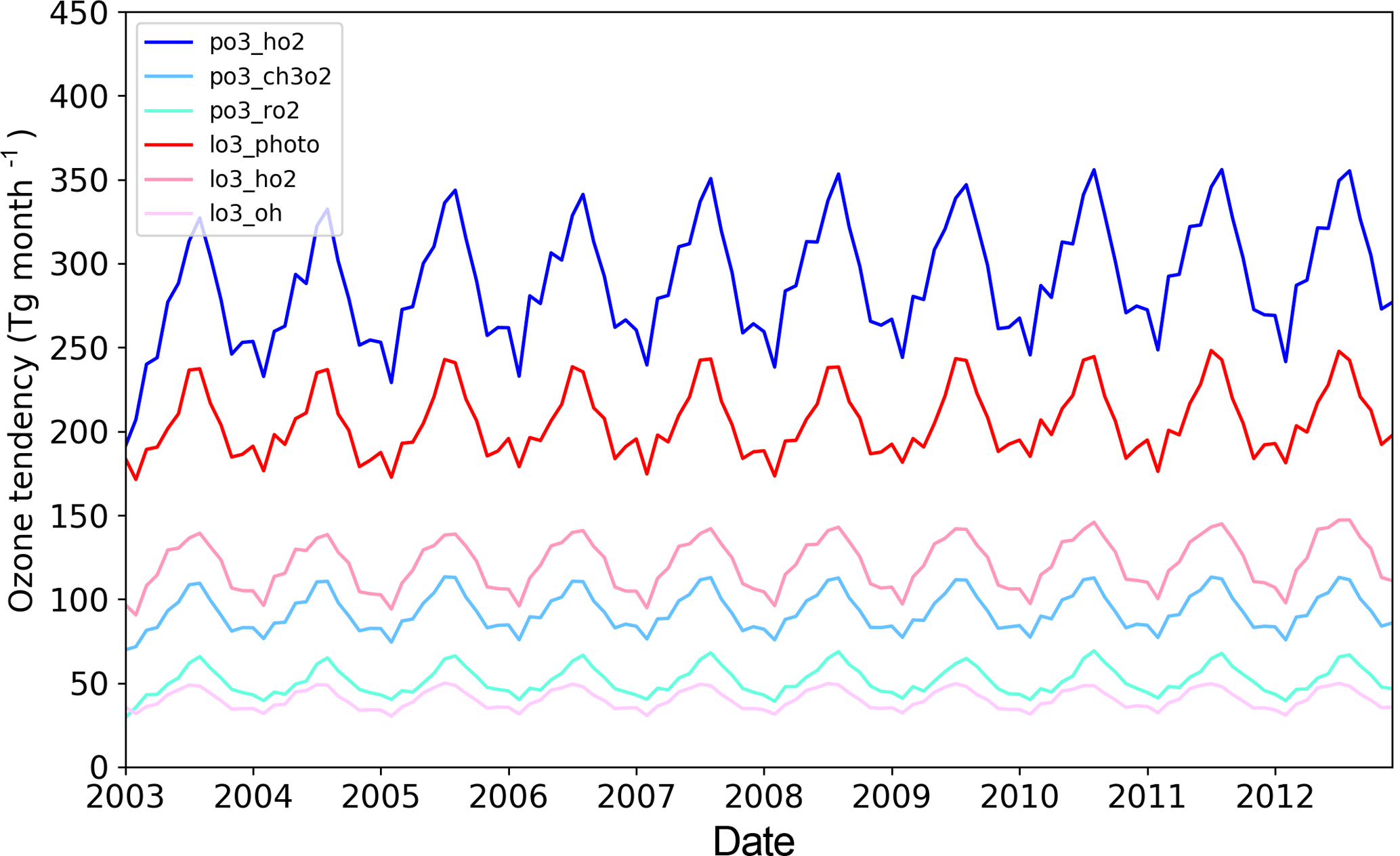
Figure 12Decadal variation in the major tropospheric ozone chemical production and loss terms from the ECHAM-HAMMOZ reference simulation. Blueish colors represent the global ozone production rates (in Tg month−1) due to the reaction of HO2, CH3O2, and other organic peroxy radicals (RO2); reddish colors show ozone loss rates due to the photolysis and subsequent reaction of O(1D) with water, due to the reaction of ozone with HO2, and due to reaction with OH.

Figure 13Decadal mean bias of total precipitation in ECHAM6.3 compared to the ECMWF ERA-Interim reanalysis (Dee et al., 2011). Gray shading denotes areas that are not significant according to a t test (95 % confidence interval). Figure regenerated from data described in Krefting (2017).
6.2 NOx budget
The global NOx budget of the base run differs somewhat from other estimates (e.g., Xu and Penner, 2012) as can be seen from Table 7. While the total NOx emissions (except for lightning as discussed above) are very similar to other recent studies, the dry and wet deposition rates are about a factor of 2 lower. This is due to the parameterization of the heterogeneous uptake of HNO3 on sea salt and dust aerosols, which removes HNO3 from the system and does not allow for reevaporation from the aerosol or droplet phase. The sensitivity run no_het_HNO3 yields dry and wet deposition rates of nitrogen that are very close to Xu and Penner (2012) and other model studies.
Xu and Penner (2012)Table 7Global tropospheric NOx budgets of the four ECHAM-HAMMOZ simulations described in Table 4.
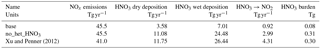
Xu and Penner (2012) distinguish between gas-phase and aerosol nitrate, while ECHAM-HAMMOZ does not have aerosol nitrate as a separate tracer. The deposition rates listed in this table are total nitrate deposition.
6.3 Radiation, clouds, and aerosol
Even though the focus of this paper is the tropospheric and stratospheric gas-phase chemistry in ECHAM-HAMMOZ, it is useful to evaluate aerosol burdens and cloud and radiation fields in order to assess how the comprehensive gas-phase chemistry mechanism of MOZ relates to HAM-only simulations and other studies. This section focuses on 10-year global mean values of radiation, cloud, and aerosol variables. Spatial distribution maps of speciated aerosol mass burdens and time series of seasonal aerosol burden means are contained in the Supplement. A more extensive evaluation of the radiation, clouds, and aerosols in ECHAM6.3-HAM2.3 will be provided in the forthcoming papers of Tegen et al. (2018), Kokkola et al. (2018), Kühn et al. (2018), and Neubauer et al. (2018).
As a baseline for the following discussion, we use the ECHAM6.3-HAM2.3 simulation of Tegen et al. (2018) and an ECHAM6.1-HAM2.2 simulation from Zhang et al. (2014). The setups of these simulations differ from the ECHAM-HAMMOZ reference simulation described in this study. Not only were the ECHAM-HAM model versions run without the gas-phase module MOZ1.0, but a different setup for the nudging was also applied in both cases (temperature was not nudged for reasons described in Zhang et al. (2014); the nudging of surface pressure, vorticity, and divergence is similar to that of our ECHAM-HAMMOZ simulations). While the ECHAM-HAM simulations were specifically tuned to bring the TOA shortwave and longwave fluxes into the observed range (Hourdin et al., 2017), no special tuning was performed for the ECHAM-HAMMOZ base simulation. Furthermore, the ECHAM6.3-HAM2.3 simulation uses a different parameterization for the emission of sea salt aerosol particles (Long et al., 2011) than ECHAM6.1-HAM2.2 and the ECHAM-HAMMOZ reference simulation, which both use the parameterization from Guelle et al. (2001). Finally, the simulation period of ECHAM6.1-HAM2.2 covers the years 2000 to 2009, whereas ECHAM6.3-HAM2.3 and ECHAM-HAMMOZ were run from 2003 to 2012. Therefore, the purpose of the following comparisons is not specifically to evaluate the impact of gas-phase chemistry on aerosols, clouds, and radiation, but rather to provide a “sanity check” for ECHAM-HAMMOZ and place the simulations that are described in this study in context with the HAM literature.
Table 8Global annual mean top of the atmosphere (TOA) energy budget, cloud-related properties, and aerosol mass burdens of the ECHAM-HAMMOZ base simulation, the ECHAM6.3-HAM2.1 (E63H23) and ECHAM6.1-HAM2.2 (E61H22) climate simulations of Tegen et al. (2018), and observations or multi-model mean values.
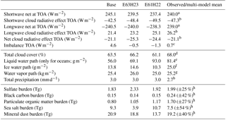
a Taken from Fig. 1 of Wild et al. (2013). b Taken from Fig. 7.7 in Boucher et al. (2013); see references therein. c Johnson et al. (2016). d Stubenrauch et al. (2013). e Elsaesser et al. (2017). f Taken from Fig. 2 of Li et al. (2012). g Average of Table S1 of von der Haar et al. (2012). h Taken from Table 10 of Textor et al. (2006).
Global 10-year mean values of the top of the atmosphere (TOA) energy budget, cloud-related properties, and aerosol mass burdens are shown in Table 8 for the ECHAM-HAMMOZ reference simulation, the ECHAM6.1-HAM2.2 and ECHAM6.3-HAM2.3 simulations, and for a blend of observations and AeroCom multi-model mean values. The table footnotes provide references for each comparison. Maps showing the spatial distribution of aerosol burden can be found in Fig. S3.6 of the Supplement, and time series of aerosol burden are presented in Fig. S3.7.
The shortwave (SW) and longwave (LW) cloud radiative effects (CREs) are weaker in the ECHAM-HAMMOZ simulation than in ECHAM6.3-HAM2.3 and in the observations. The differences in SWCRE (LWCRE) are −6 W m−2 (−2 W m−2) with respect to ECHAM6.3-HAM2.3 and −5 W m−2 (−5 W m−2) with respect to the observations. These differences can be explained by a lower cloud cover and a smaller liquid water path in the ECHAM-HAMMOZ simulation. They are similar to differences observed between different ECHAM6.1-HAM2.2 simulations described in Zhang et al. (2014), in which different setups of the nudging were tested and compared to free-running simulations constrained only by sea surface temperature and sea ice cover. For ECHAM6.1-HAM2.2 they found a decrease in SWCRE (LWCRE) by about 5 W m−2 (1 W m−2) together with a decrease in the liquid water path by about 10 g m−2 when temperature was included in the nudging parameters. Additional impacts of nudging were seen in the water vapor path and in convective clouds. It is therefore likely that the differences in cloud and radiation fields between ECHAM-HAMMOZ and ECHAM-HAM can be explained by the different nudging setups used, although the different model tuning may also play a role here.
The differences in SWCRE and LWCRE lead to larger net shortwave TOA fluxes and an imbalance of the radiative TOA fluxes of 4.6 W m−2, which is somewhat larger than the imbalances found in the two ECHAM-HAM simulations or in Johnson et al. (2016).
The 10-year global means of the aerosol mass burdens of the ECHAM-HAMMOZ simulations are comparable with the ECHAM-HAM simulations and AeroCom multi-model mean values of Textor et al. (2006). The particulate organic matter (POM) burdens in all ECHAM-HAM(MOZ) simulations are lower than in the AeroCom multi-model mean, which could be due to the simplistic treatment of secondary organic aerosols (Zhang et al., 2012). The POM burden in the base run is even lower than in the two comparison simulations. The reasons for this are not clear at present. Compared to ECHAM6.3-HAM2.3 the sea salt burdens in ECHAM-HAMMOZ and ECHAM6.1-HAM2.2 are substantially larger. This difference results from changing the sea salt emission scheme from Guelle et al. (2001) to Long et al. (2011) as described above. The multi-model mean from AeroCom (Textor et al., 2006) falls in between the two ECHAM-HAM versions.
Overall, the 10-year mean aerosol burden maps (Fig. S3.5) show a reasonable comparison between the patterns of ECHAM-HAMMOZ and ECHAM6.3HAM2.3. The gas-phase module MOZ1.0 in ECHAM-HAMMOZ does not interact directly with black carbon, particulate organic matter, sea salt, and mineral dust. However, the formation of sulfate aerosol is different (gas-phase H2SO4 is explicitly included in MOZ1.0, whereas it is parameterized in HAM) so that the largest differences between ECHAM-HAMMOZ and ECHAM6-HAM2.3 are expected for sulfate aerosol. Indeed, the sulfate burden (first row of Fig. S3.5) is lower everywhere in ECHAM-HAMMOZ than in ECHAM6.3-HAM2.3, but is quite comparable to ECHAM6.1-HAM2.2. The differences between the different ECHAM-HAM(MOZ) versions are in the range of the AeroCom models. The spatial distributions of black carbon, particulate organic matter, and mineral dust burdens are quite similar in ECHAM-HAMMOZ compared to ECHAM6.3-HAM2.3. For the sea salt burden, the spatial distribution of ECHAM-HAMMOZ agrees well with the one of ECHAM6.1-HAM2.2. The seasonal cycles of the global means of aerosol mass burdens in ECHAM-HAMMOZ are very similar to the ones in ECHAM6.3-HAM2.3 and ECHAM6.1-HAM2.2 (Fig. S3.6 in the Supplement). The differences are consistent with those discussed above.
Overall, it can be concluded that the nudged ECHAM-HAMMOZ base simulation produces reasonable results for TOA radiative fluxes, cloud-related properties, and aerosol mass burdens. All parameters are in the range of other nudged ECHAM-HAM simulations, AeroCom multi-model mean values, and observations. Differences between ECHAM-HAMMOZ and ECHAM6.3-HAM2.3 can be explained primarily by the different model setup, i.e., the use of a different sea salt emissions scheme (see also Tegen et al., 2018), and different settings for the dynamical nudging (Zhang et al., 2014). The largest direct impact of using the gas-phase module MOZ1.0 that could be identified is a 21 % decrease in sulfate aerosol mass burden, which is within the range of AeroCom models. A more thorough evaluation of the impact of using MOZ1.0 could be achieved by comparing model configurations with and without MOZ1.0 using an otherwise identical model setup, but this is beyond the scope of this study.
Shorter test simulations with the SALSA microphysics package reveal minor differences compared to the M7 simulations presented in this work (Stadtler et al., 2018).
ECHAM-HAMMOZ in its released version ECHAM6.3-HAM2.3-MOZ1.0 is a state-of-the-art chemistry–climate model with a comprehensive tropospheric and stratospheric chemistry package and two options to model aerosol processes with either a modal or a bin scheme.
A 10-year simulation from 2003 to 2012 in the default configuration was performed and has been evaluated with various observational data and compared to other model studies. The focus of the evaluation was placed on the year 2008. The model reproduces many of the observed features of total column ozone, polar stratospheric processes, tropospheric and surface ozone, and column and surface CO. Like many other models, ECHAM-HAMMOZ shows a high bias of surface ozone concentrations, but this bias is relatively modest. Global budgets of ozone and OH are in line with estimates from multi-model intercomparison studies and two individual models using either a similar chemistry scheme (CAM-CHEM) or a similar climate model (EMAC) as ECHAM-HAMMOZ.
The evaluation of the model run in the default configuration revealed two issues with respect to the global NOx budget: (1) lightning emissions are only about 1.2 Tg(N) yr−1 and thus a factor of 2 lower than the lower limit that is generally accepted by the community; and (2) the parameterizations of heterogeneous reactions constitute a too-strong sink of HNO3. The aerosol model of ECHAM-HAMMOZ does not include an explicit treatment of nitrate, and therefore the reevaporation of HNO3 that is lost to the aerosol phase does not occur. Three sensitivity simulations were performed, which corrected these issues. Unfortunately, the results from these simulations tend to increase model biases, and they particularly invigorate the tropospheric ozone chemistry and decrease the lifetime of CH4. These changes occur almost exclusively in the tropics and may be related to issues with tropical dynamics in the ECHAM model, which also show up as precipitation bias. The evaluation of cloud and radiation budgets hints towards a possible radiative imbalance induced by the nudging setup. However, the precipitation bias has also been found in other simulations with ECHAM6, and the excessive ozone chemistry and OH concentrations are also a feature of EMAC, which is based on an earlier version of ECHAM (with modifications).
The ECHAM-HAMMOZ model source code and all required input data are freely available after signature of a license agreement. Further information and the license agreement can be obtained from https://dx.doi.org/11097/24231152-1f57-425a-911b-701b49b5958c (Schultz et al., 2018a), and more detailed stratospheric diagnostics can be obtained from https://dx.doi.org/11097/54c0ad1d-cc58-466e-a32a-c0391753e06f (Schultz et al., 2018b). The IASI products used in this paper are available from the ULB authors upon request.
The supplement related to this article is available online at: https://doi.org/10.5194/gmd-11-1695-2018-supplement.
MGS participated in the general code design of ECHAM-HAMMOZ and led the development of the gas-phase chemistry module; he designed this paper, performed 30 % of the analyses, and wrote 65 % of the paper. ScS contributed to the model development, performed most model simulations, and contributed to the analysis. SaS and SF were pivotal in the technical model development and maintenance of all prior code versions. CSLD managed the model input data and contributed to the model development. All other authors contributed either to the model development or to the model evaluation and contributed individual sections to the paper.
The authors declare that they have no conflict of interest.
The ECHAM-HAMMOZ model is developed by a consortium composed of ETH Zurich,
the Max-Planck-Institut für Meteorologie, Forschungszentrum Jülich, the
University of Oxford, the Finnish Meteorological Institute, and the Leibniz
Institute for Tropospheric Research and managed by the Center for Climate
Systems Modeling (C2SM) at ETH Zurich. We wish to thank the C2SM at ETH
Zurich for hosting the model code and technical support for the model
development. JSC is acknowledged for computing time on JURECA (2016) and
technical support for the implementation of the model on this platform.
Specifically, we would like to thank Olaf Stein for his continuous support.
The Max Planck Institute for Meteorology in Hamburg, Germany is gratefully
acknowledged for developing the ECHAM general circulation model and making it
available to the HAMMOZ community. Charles Bardeen (NCAR) helped to make MLS
data available for the evaluation of stratospheric processes. All authors
from Forschungszentrum Jülich have been funded through the Helmholtz POF
program. PS acknowledges funding from the European Union's Seventh Framework
Programme (FP7/2007-2013) projects BACCHUS under grant agreement 603445 and
the European Research Council project RECAP under the European Union's
Horizon 2020 research and innovation program with grant agreement
724602. The research at ULB is
funded by the Belgian State Federal Office for Scientific, Technical and
Cultural Affairs and the European Space Agency (ESA Prodex IASI Flow and AC
SAF). The authors are grateful to Daniel Hurtmans (ULB) for developing and
maintaining FORLI.
Edited by: Fiona O'Connor
Reviewed by: three anonymous referees
Abdul-Razzak, H. and Ghan, S. J.: A parameterization of aerosol activation: 2. Multiple aerosol types, J. Geophys. Res.-Atmos., 105, 6837–6844, https://doi.org/10.1029/1999JD901161, 2000. a
Aghedo, A. M., Schultz, M. G., and Rast, S.: The influence of African air pollution on regional and global tropospheric ozone, Atmos. Chem. Phys., 7, 1193–1212, https://doi.org/10.5194/acp-7-1193-2007, 2007. a
Austin, J., Garcia, R. R., Russell III, J. M., Solomon, S., and Tuck, A. F.: On the atmospheric photochemistry of nitric acid, J. Geophys. Res.-Atmos., 91, 5477–5485, https://doi.org/10.1029/JD091iD05p05477, 1986. a
Auvray, M., Bey, I., Llull, E., Schultz, M. G., and Rast, S.: A model investigation of tropospheric ozone chemical tendencies in long-range transported pollution plumes, Journal of Geophysical Research: Atmospheres, 112, d05304, https://doi.org/10.1029/2006JD007137, 2007. a
Baumgaertner, A. J. G., Jöckel, P., Kerkweg, A., Sander, R., and Tost, H.: Implementation of the Community Earth System Model (CESM) version 1.2.1 as a new base model into version 2.50 of the MESSy framework, Geosci. Model Dev., 9, 125–135, https://doi.org/10.5194/gmd-9-125-2016, 2016. a
Bergman, T., Kerminen, V.-M., Korhonen, H., Lehtinen, K. J., Makkonen, R., Arola, A., Mielonen, T., Romakkaniemi, S., Kulmala, M., and Kokkola, H.: Evaluation of the sectional aerosol microphysics module SALSA implementation in ECHAM5-HAM aerosol-climate model, Geosci. Model Dev., 5, 845–868, https://doi.org/10.5194/gmd-5-845-2012, 2012. a
Boccippio, D. J., Goodman, S. J., and Heckman, S.: Regional Differences in Tropical Lightning Distributions, J. Appl. Meteorol., 39, 2231–2248, https://doi.org/10.1175/1520-0450(2001)040<2231:RDITLD>2.0.CO;2, 2000. a
Boucher, O., Randall, D., Artaxo, P., Bretherton, C., Feingold, G., Forster, P., Kerminen, V.-M., Kondo, Y., Liao, H., Lohmann, U., Rasch, P., Satheesh, S., Sherwood, S., Stevens, B., and Zhang, X.: Clouds and aerosols, Cambridge University Press, 571–657, 2013. a
Boynard, A., Hurtmans, D., Koukouli, M. E., Goutail, F., Bureau, J., Safieddine, S., Lerot, C., Hadji-Lazaro, J., Wespes, C., Pommereau, J.-P., Pazmino, A., Zyrichidou, I., Balis, D., Barbe, A., Mikhailenko, S. N., Loyola, D., Valks, P., Van Roozendael, M., Coheur, P.-F., and Clerbaux, C.: Seven years of IASI ozone retrievals from FORLI: validation with independent total column and vertical profile measurements, Atmos. Meas. Tech., 9, 4327–4353, https://doi.org/10.5194/amt-9-4327-2016, 2016. a
Boynard, A., Hurtmans, D., Garane, K., Goutail, F., Hadji-Lazaro, J., Koukouli, M. E., Wespes, C., Keppens, A., Pommereau, J.-P., Pazmino, A., Balis, D., Loyola, D., Valks, P., Coheur, P.-F., and Clerbaux, C.: Validation of the IASI FORLI/Eumetsat ozone products using satellite (GOME-2), ground-based (Brewer-Dobson, SAOZ) and ozonesonde measurements, Atmos. Meas. Tech. Discuss., https://doi.org/10.5194/amt-2017-461, in review, 2018. a, b
Brasseur, G. P., Hauglustaine, D. A., Walters, S., Rasch, P. J., Muller, J. F., Granier, C., and Tie, X. X.: MOZART, a global chemical transport model for ozone and related chemical tracers 1. Model description, J. Geophys. Res.-Atmos., 103, 28265–28289, https://doi.org/10.1029/98jd02397, 1998. a
Brinkop, S. and Roeckner, E.: Sensitivity of a general-circulation model to parameterizations of cloud-turbulence interactions in the atmospheric boundary-layer, Tellus A, 47, 197–220, https://doi.org/10.1034/j.1600-0870.1995.t01-1-00004.x, 1995. a
Brovkin, V., Boysen, L., Raddatz, T., Gayler, V., Loew, A., and Claussen, M.: Evaluation of vegetation cover and land-surface albedo in MPI-ESM CMIP5 simulations, J. Adv. Model. Earth Sy., 5, 48–57, https://doi.org/10.1029/2012ms000169, 2013. a
Christian, H. J., Blakeslee, R. J., Boccippio, D. J., Boeck, W. L., Buechler, D. E., Driscoll, K. T., Goodman, S. J., Hall, J. M., Koshak, W. J., Mach, D. M., and Stewart, M. F.: Global frequency and distribution of lightning as observed from space by the Optical Transient Detector, J. Geophys. Res.-Atmos., 108, 4005, https://doi.org/10.1029/2002jd002347, 2003. a
Clerbaux, C., Boynard, A., Clarisse, L., George, M., Hadji-Lazaro, J., Herbin, H., Hurtmans, D., Pommier, M., Razavi, A., Turquety, S., Wespes, C., and Coheur, P.-F.: Monitoring of atmospheric composition using the thermal infrared IASI/MetOp sounder, Atmos. Chem. Phys., 9, 6041–6054, https://doi.org/10.5194/acp-9-6041-2009, 2009. a
Croft, B., Lohmann, U., Martin, R. V., Stier, P., Wurzler, S., Feichter, J., Posselt, R., and Ferrachat, S.: Aerosol size-dependent below-cloud scavenging by rain and snow in the ECHAM5-HAM, Atmos. Chem. Phys., 9, 4653–4675, https://doi.org/10.5194/acp-9-4653-2009, 2009. a
Croft, B., Lohmann, U., Martin, R. V., Stier, P., Wurzler, S., Feichter, J., Hoose, C., Heikkilä, U., van Donkelaar, A., and Ferrachat, S.: Influences of in-cloud aerosol scavenging parameterizations on aerosol concentrations and wet deposition in ECHAM5-HAM, Atmos. Chem. Phys., 10, 1511–1543, https://doi.org/10.5194/acp-10-1511-2010, 2010. a
Dee, D. P., Uppala, S. M., Simmons, A. J., Berrisford, P., Poli, P., Kobayashi, S., Andrae, U., Balmaseda, M. A., Balsamo, G., Bauer, P., Bechtold, P., Beljaars, A. C. M., van de Berg, L., Bidlot, J., Bormann, N., Delsol, C., Dragani, R., Fuentes, M., Geer, A. J., Haimberger, L., Healy, S. B., Hersbach, H., Holm, E. V., Isaksen, L., Kallberg, P., Kohler, M., Matricardi, M., McNally, A. P., Monge-Sanz, B. M., Morcrette, J. J., Park, B. K., Peubey, C., de Rosnay, P., Tavolato, C., Thepaut, J. N., and Vitart, F.: The ERA-Interim reanalysis: configuration and performance of the data assimilation system, Q. J. Roy. Meteor. Soc., 137, 553–597, https://doi.org/10.1002/qj.828, 2011. a, b, c
Dentener, F., Kinne, S., Bond, T., Boucher, O., Cofala, J., Generoso, S., Ginoux, P., Gong, S., Hoelzemann, J. J., Ito, A., Marelli, L., Penner, J. E., Putaud, J.-P., Textor, C., Schulz, M., van der Werf, G. R., and Wilson, J.: Emissions of primary aerosol and precursor gases in the years 2000 and 1750 prescribed data-sets for AeroCom, Atmos. Chem. Phys., 6, 4321–4344, https://doi.org/10.5194/acp-6-4321-2006, 2006a. a
Dentener, F., Stevenson, D., Ellingsen, K., van Noije, T., Schultz, M., Amann, M., Atherton, C., Bell, N., Bergmann, D., Bey, I., Bouwman, L., Butler, T., Cofala, J., Collins, B., Drevet, J., Doherty, R., Eickhout, B., Eskes, H., Fiore, A., Gauss, M., Hauglustaine, D., Horowitz, L., Isaksen, I. S. A., Josse, B., Lawrence, M., Krol, M., Lamarque, J. F., Montanaro, V., Muller, J. F., Peuch, V. H., Pitari, G., Pyle, J., Rast, S., Rodriguez, J., Sanderson, M., Savage, N. H., Shindell, D., Strahan, S., Szopa, S., Sudo, K., Van Dingenen, R., Wild, O., and Zeng, G.: The global atmospheric environment for the next generation, Environ. Sci. Technol., 40, 3586–3594, https://doi.org/10.1021/es0523845, 2006b. a, b
Elsaesser, G. S., O'Dell, C. W., Lebsock, M. D., Bennartz, R., Greenwald, T. J., and Wentz, F. J.: The Multisensor Advanced Climatology of Liquid Water Path (MAC-LWP), J. Climate, 30, 10193–10210, https://doi.org/10.1175/JCLI-D-16-0902.1, 2017. a
Emmons, L. K., Apel, E. C., Lamarque, J.-F., Hess, P. G., Avery, M., Blake, D., Brune, W., Campos, T., Crawford, J., DeCarlo, P. F., Hall, S., Heikes, B., Holloway, J., Jimenez, J. L., Knapp, D. J., Kok, G., Mena-Carrasco, M., Olson, J., O'Sullivan, D., Sachse, G., Walega, J., Weibring, P., Weinheimer, A., and Wiedinmyer, C.: Impact of Mexico City emissions on regional air quality from MOZART-4 simulations, Atmos. Chem. Phys., 10, 6195–6212, https://doi.org/10.5194/acp-10-6195-2010, 2010. a, b
Eskes, H., Huijnen, V., Arola, A., Benedictow, A., Blechschmidt, A.-M., Botek, E., Boucher, O., Bouarar, I., Chabrillat, S., Cuevas, E., Engelen, R., Flentje, H., Gaudel, A., Griesfeller, J., Jones, L., Kapsomenakis, J., Katragkou, E., Kinne, S., Langerock, B., Razinger, M., Richter, A., Schultz, M., Schulz, M., Sudarchikova, N., Thouret, V., Vrekoussis, M., Wagner, A., and Zerefos, C.: Validation of reactive gases and aerosols in the MACC global analysis and forecast system, Geoscientific Model Development, 8, 3523–3543, https://doi.org/10.5194/gmd-8-3523-2015, 2015. a
Eyring, V., Arblaster, J. M., Cionni, I., Sedlacek, J., Perliwitz, J., Young, P. J., Bekki, S., Bergmann, D., Cameron-Smith, P., Collins, W. J., Faluvegi, G., Gottschaldt, K. D., Horowitz, L. W., Kinnison, D. E., Lamarque, J. F., Marsh, D. R., Saint-Martin, D., Shindell, D. T., Sudo, K., Szopa, S., and Watanabe, S.: Long-term ozone changes and associated climate impacts in CMIP5 simulations, J. Geophys. Res.-Atmos., 118, 5029–5060, https://doi.org/10.1002/jgrd.50316, 2013. a
Fadnavis, S., Semeniuk, K., Pozzoli, L., Schultz, M. G., Ghude, S. D., Das, S., and Kakatkar, R.: Transport of aerosols into the UTLS and their impact on the Asian monsoon region as seen in a global model simulation, Atmos. Chem. Phys., 13, 8771–8786, https://doi.org/10.5194/acp-13-8771-2013, 2013. a
Fadnavis, S., Schultz, M. G., Semeniuk, K., Mahajan, A. S., Pozzoli, L., Sonbawne, S., Ghude, S. D., Kiefer, M., and Eckert, E.: Trends in peroxyacetyl nitrate (PAN) in the upper troposphere and lower stratosphere over southern Asia during the summer monsoon season: regional impacts, Atmos. Chem. Phys., 14, 12725–12743, https://doi.org/10.5194/acp-14-12725-2014, 2014. a
Fadnavis, S., Semeniuk, K., Schultz, M. G., Kiefer, M., Mahajan, A., Pozzoli, L., and Sonbawane, S.: Transport pathways of peroxyacetyl nitrate in the upper troposphere and lower stratosphere from different monsoon systems during the summer monsoon season, Atmos. Chem. Phys., 15, 11477–11499, https://doi.org/10.5194/acp-15-11477-2015, 2015. a
Ganzeveld, L. and Lelieveld, J.: Dry deposition parameterization in a chemistry general-circulation model and its influence on the distribution of reactive trace gases, J. Geophys. Res.-Atmos., 100, 20999–21012, https://doi.org/10.1029/95jd02266, 1995. a
Gelaro, R., McCarty, W., Suárez, M. J., Todling, R., Molod, A., Takacs, L., Randles, C. A., Darmenov, A., Bosilovich, M. G., Reichle, R., Wargan, K., Coy, L., Cullather, R., Draper, C., Akella, S., Buchard, V., Conaty, A., da Silva, A. M., Gu, W., Kim, G.-K., Koster, R., Lucchesi, R., Merkova, D., Nielsen, J. E., Partyka, G., Pawson, S., Putman, W., Rienecker, M., Schubert, S. D., Sienkiewicz, M., and Zhao, B.: The Modern-Era Retrospective Analysis for Research and Applications, Version 2 (MERRA-2), J. Climate, 30, 5419–5454, https://doi.org/10.1175/JCLI-D-16-0758.1, 2017. a, b
George, M., Clerbaux, C., Bouarar, I., Coheur, P.-F., Deeter, M. N., Edwards, D. P., Francis, G., Gille, J. C., Hadji-Lazaro, J., Hurtmans, D., Inness, A., Mao, D., and Worden, H. M.: An examination of the long-term CO records from MOPITT and IASI: comparison of retrieval methodology, Atmos. Meas. Tech., 8, 4313–4328, https://doi.org/10.5194/amt-8-4313-2015, 2015. a, b
Ghan, S., Wang, M. H., Zhang, S. P., Ferrachat, S., Gettelman, A., Griesfeller, J., Kipling, Z., Lohmann, U., Morrison, H., Neubauer, D., Partridge, D. G., Stier, P., Takemura, T., Wang, H. L., and Zhang, K.: Challenges in constraining anthropogenic aerosol effects on cloud radiative forcing using present-day spatiotemporal variability, P. Natl. Acad. Sci. USA, 113, 5804–5811, https://doi.org/10.1073/pnas.1514036113, 2016. a
Giorgetta, M., Jungclaus, J., Reick, C., Legutke, S., Brovkin, V., Crueger, T., Esch, M., Fieg, K., Glushak, K., Gayler, V., Haak, H., Hollweg, H.-D., Kinne, S., Kornblueh, L., Matei, D., Mauritsen, T., Mikolajewicz, U., Müller, W., Notz, D., Raddatz, T., Rast, S., Roeckner, E., Salzmann, M., Schmidt, H., Schnur, R., Segschneider, J., Six, K., Stockhause, M., Wegner, J., Widmann, H., Wieners, K.-H., Claussen, M., Marotzke, J., and Stevens, B.: CMIP5 simulations of the Max Planck Institute for Meteorology (MPI-M) based on the MPI-ESM-LR model: The amip experiment, served by ESGF, World Data Center for Climate (WDCC) at DKRZ, https://doi.org/10.1594/WDCC/CMIP5.MXELam, 2012. a
Granier, C., Guenther, A., Lamarque, J., Mieville, A., Muller, J., Olivier, J., Orlando, J., Peters, J., Petron, G., Tyndall, G., and Wallens, S.: POET, a database of surface emissions of ozone precursors, available at: http://www.aero.jussieu.fr/projet/ACCENT/POET.php (last access: 20 April 2018), 2005. a
Granier, C., Bessagnet, B., Bond, T., D'Angiola, A., van der Gon, H. D., Frost, G. J., Heil, A., Kaiser, J. W., Kinne, S., Klimont, Z., Kloster, S., Lamarque, J. F., Liousse, C., Masui, T., Meleux, F., Mieville, A., Ohara, T., Raut, J. C., Riahi, K., Schultz, M. G., Smith, S. J., Thompson, A., van Aardenne, J., van der Werf, G. R., and van Vuuren, D. P.: Evolution of anthropogenic and biomass burning emissions of air pollutants at global and regional scales during the 1980–2010 period, Climatic Change, 109, 163–190, https://doi.org/10.1007/s10584-011-0154-1, 2011. a
Grewe, V., Brunner, D., Dameris, M., Grenfell, J. L., Hein, R., Shindell, D., and Staehelin, J.: Origin and variability of upper tropospheric nitrogen oxides and ozone at northern mid-latitudes, Atmos. Environ., 35, 3421–3433, https://doi.org/10.1016/s1352-2310(01)00134-0, 2001. a
Guelle, W., Schulz, M., Balkanski, Y., and Dentener, F.: Influence of the source formulation on modeling the atmospheric global distribution of sea salt aerosol, J. Geophys. Res.-Atmos., 106, 27509–27524, https://doi.org/10.1029/2001jd900249, 2001. a, b, c
Guenther, A. B., Jiang, X., Heald, C. L., Sakulyanontvittaya, T., Duhl, T., Emmons, L. K., and Wang, X.: The Model of Emissions of Gases and Aerosols from Nature version 2.1 (MEGAN2.1): an extended and updated framework for modeling biogenic emissions, Geosci. Model Dev., 5, 1471–1492, https://doi.org/10.5194/gmd-5-1471-2012, 2012. a, b
Gutman, G., Tarpley, D., Ignatov, A., and Olson, S.: The enhanced noaa global land dataset from the advanced very high-resolution radiometer, B. Am. Meteorol. Soc., 76, 1141–1156, https://doi.org/10.1175/1520-0477(1995)076<1141:tengld>2.0.co;2, 1995. a
Hagemann, S. and Stacke, T.: Impact of the soil hydrology scheme on simulated soil moisture memory, Clim. Dynam., 44, 1731–1750, https://doi.org/10.1007/s00382-014-2221-6, 2015. a
Harrison, J. J., Chipperfield, M. P., Boone, C. D., Dhomse, S. S., Bernath, P. F., Froidevaux, L., Anderson, J., and Russell III, J.: Satellite observations of stratospheric hydrogen fluoride and comparisons with SLIMCAT calculations, Atmos. Chem. Phys., 16, 10501–10519, https://doi.org/10.5194/acp-16-10501-2016, 2016. a
Henrot, A.-J., Stanelle, T., Schröder, S., Siegenthaler, C., Taraborrelli, D., and Schultz, M. G.: Implementation of the MEGAN (v2.1) biogenic emission model in the ECHAM6-HAMMOZ chemistry climate model, Geosci. Model Dev., 10, 903–926, https://doi.org/10.5194/gmd-10-903-2017, 2017. a, b
Hines, C. O.: Doppler-spread parameterization of gravity-wave momentum deposition in the middle atmosphere. Part 1: Basic formulation, J. Atmos. Sol.-Terr. Phys., 59, 371–386, https://doi.org/10.1016/S1364-6826(96)00079-X, 1997a. a
Hines, C. O.: Doppler-spread parameterization of gravity-wave momentum deposition in the middle atmosphere. Part 2: Broad and quasi monochromatic spectra, and implementation, J. Atmos. Sol.-Terr. Phys., 59, 387–400, https://doi.org/10.1016/s1364-6826(96)00080-6, 1997b. a
Hourdin, F., Mauritsen, T., Gettelman, A., Golaz, J.-C., Balaji, V., Duan, Q., Folini, D., Ji, D., Klocke, D., Qian, Y., Rauser, F., Rio, C., Tomassini, L., Watanabe, M., and Williamson, D.: The Art and Science of Climate Model Tuning, B. Am. Meteorol. Soc., 98, 589–602, https://doi.org/10.1175/BAMS-D-15-00135.1, 2017. a
Hurtmans, D., Coheur, P.-F., Wespes, C., Clarisse, L., Scharf, O., Clerbaux, C., Hadji-Lazaro, J., George, M., and Turquety, S.: FORLI radiative transfer and retrieval code for IASI, J. Quant. Spectrosc. Ra., 113, 1391–1408, https://doi.org/10.1016/j.jqsrt.2012.02.036, 2012. a, b, c
Iacono, M. J., Delamere, J. S., Mlawer, E. J., Shephard, M. W., Clough, S. A., and Collins, W. D.: Radiative forcing by long-lived greenhouse gases: Calculations with the AER radiative transfer models, J. Geophys. Res.-Atmos., 113, d13103, https://doi.org/10.1029/2008JD009944, 2008. a
Inness, A., Baier, F., Benedetti, A., Bouarar, I., Chabrillat, S., Clark, H., Clerbaux, C., Coheur, P., Engelen, R. J., Errera, Q., Flemming, J., George, M., Granier, C., Hadji-Lazaro, J., Huijnen, V., Hurtmans, D., Jones, L., Kaiser, J. W., Kapsomenakis, J., Lefever, K., Leitão, J., Razinger, M., Richter, A., Schultz, M. G., Simmons, A. J., Suttie, M., Stein, O., Thépaut, J.-N., Thouret, V., Vrekoussis, M., Zerefos, C., and the MACC team: The MACC reanalysis: an 8 yr data set of atmospheric composition, Atmos. Chem. Phys., 13, 4073–4109, https://doi.org/10.5194/acp-13-4073-2013, 2013. a
Jenkin, M. E., Young, J. C., and Rickard, A. R.: The MCM v3.3.1 degradation scheme for isoprene, Atmos. Chem. Phys., 15, 11433–11459, https://doi.org/10.5194/acp-15-11433-2015, 2015. a
Jiao, C., Flanner, M. G., Balkanski, Y., Bauer, S. E., Bellouin, N., Berntsen, T. K., Bian, H., Carslaw, K. S., Chin, M., De Luca, N., Diehl, T., Ghan, S. J., Iversen, T., Kirkevåg, A., Koch, D., Liu, X., Mann, G. W., Penner, J. E., Pitari, G., Schulz, M., Seland, Ø., Skeie, R. B., Steenrod, S. D., Stier, P., Takemura, T., Tsigaridis, K., van Noije, T., Yun, Y., and Zhang, K.: An AeroCom assessment of black carbon in Arctic snow and sea ice, Atmos. Chem. Phys., 14, 2399–2417, https://doi.org/10.5194/acp-14-2399-2014, 2014. a
Jöckel, P., Tost, H., Pozzer, A., Kunze, M., Kirner, O., Brenninkmeijer, C. A. M., Brinkop, S., Cai, D. S., Dyroff, C., Eckstein, J., Frank, F., Garny, H., Gottschaldt, K.-D., Graf, P., Grewe, V., Kerkweg, A., Kern, B., Matthes, S., Mertens, M., Meul, S., Neumaier, M., Nützel, M., Oberländer-Hayn, S., Ruhnke, R., Runde, T., Sander, R., Scharffe, D., and Zahn, A.: Earth System Chemistry integrated Modelling (ESCiMo) with the Modular Earth Submodel System (MESSy) version 2.51, Geosci. Model Dev., 9, 1153–1200, https://doi.org/10.5194/gmd-9-1153-2016, 2016. a, b, c, d, e
Johnson, G. C., Lyman, J. M., and Loeb, N. G.: Correspondence: Improving estimates of Earth's energy imbalance, Nat. Clim. Change, 6, 639–640, 2016. a, b
JURECA, Jülich Supercomputing Centre.: JURECA: General-purpose supercomputer at Jülich Supercomputing Centre, Journal of large-scale research facilities, 2, A62, https://doi.org/10.17815/jlsrf-2-121, 2016. a
Kaas, E., Guldberg, A., Déqué, M., Braun, A., Piedelievre, J., Guérémy, J., Machenhauer, B., Kirchner, I., D'Andrea, F., Vautard, R., D'Andrea, F., and Corti, S.: Final report of the POTENTIALS project (Project On Tendency Evaluations using New Techniques to Improve Atmospheric Long-term Simulations), available from the EU-Commision (DGXII), 2000. a
Kinnison, D. E., Brasseur, G. P., Walters, S., Garcia, R. R., Marsh, D. R., Sassi, F., Harvey, V. L., Randall, C. E., Emmons, L., Lamarque, J. F., Hess, P., Orlando, J. J., Tie, X. X., Randel, W., Pan, L. L., Gettelman, A., Granier, C., Diehl, T., Niemeier, U., and Simmons, A. J.: Sensitivity of chemical tracers to meteorological parameters in the MOZART-3 chemical transport model, J. Geophys. Res.-Atmos., 112, D20302, https://doi.org/10.1029/2006jd007879, 2007. a, b, c, d, e, f, g
Kloster, S., Feichter, J., Maier-Reimer, E., Six, K. D., Stier, P., and Wetzel, P.: DMS cycle in the marine ocean-atmosphere system – a global model study, Biogeosciences, 3, 29–51, https://doi.org/10.5194/bg-3-29-2006, 2006. a
Kokkola, H., Korhonen, H., Lehtinen, K. E. J., Makkonen, R., Asmi, A., Järvenoja, S., Anttila, T., Partanen, A.-I., Kulmala, M., Järvinen, H., Laaksonen, A., and Kerminen, V.-M.: SALSA – a Sectional Aerosol module for Large Scale Applications, Atmos. Chem. Phys., 8, 2469–2483, https://doi.org/10.5194/acp-8-2469-2008, 2008. a
Kokkola, H., Kühn, T., Laakso, A., Bergman, T., Lehtinen, K. E. J., Mielonen, T., Arola, A., Stadtler, S., Korhonen, H., Ferrachat, S., Lohmann, U., Neubauer, D., Tegen, I., Siegenthaler-Le Drian, C., Schultz, M. G., Bey, I., Stier, P., Daskalakis, N., Heald, C. L., and Romakkaniemi, S.: SALSA2.0: The sectional aerosol module of the aerosol-chemistry-climate model ECHAM6.3.0-HAM2.3-MOZ1.0, Geosci. Model Dev. Discuss., https://doi.org/10.5194/gmd-2018-47, in review, 2018. a, b
Kühn, T., Merikanto, J., Mielonen, T., Stadtler, S., Schultz, M., Hienola, A., Korhonen, H., Ferrachat, S., Lohmann, U., Neubauer, D., Tegen, I., Drian, C. S.-L., Rast, S., Schmidt, H., Stier, P., Lehtinen, K., and Kokkola, H.: SALSA2.0 – Part 2: Implementation of a volatility basis set to model formation of secondary organic aerosol, Geosci. Model Dev. Discuss., in preparation, 2018. a
Krefting, J.: Nudging in Climate Modeling with ECHAM6.3, Master thesis, Meteorological Institute, Rheinische Friedrich-Wilhelms-Universität Bonn, 2017. a, b
Laepple, T., Schultz, M. G., Lamarque, J. F., Madronich, S., Shetter, R. E., Lefer, B. L., and Atlas, E.: Improved albedo formulation for chemistry transport models based on satellite observations and assimilated snow data and its impact on tropospheric photochemistry, J. Geophys. Res.-Atmos., 110, D11308, https://doi.org/10.1029/2004jd005463, 2005. a
Lamarque, J.-F., Bond, T. C., Eyring, V., Granier, C., Heil, A., Klimont, Z., Lee, D., Liousse, C., Mieville, A., Owen, B., Schultz, M. G., Shindell, D., Smith, S. J., Stehfest, E., Van Aardenne, J., Cooper, O. R., Kainuma, M., Mahowald, N., McConnell, J. R., Naik, V., Riahi, K., and van Vuuren, D. P.: Historical (1850–2000) gridded anthropogenic and biomass burning emissions of reactive gases and aerosols: methodology and application, Atmos. Chem. Phys., 10, 7017–7039, https://doi.org/10.5194/acp-10-7017-2010, 2010. a
Lamarque, J.-F., Emmons, L. K., Hess, P. G., Kinnison, D. E., Tilmes, S., Vitt, F., Heald, C. L., Holland, E. A., Lauritzen, P. H., Neu, J., Orlando, J. J., Rasch, P. J., and Tyndall, G. K.: CAM-chem: description and evaluation of interactive atmospheric chemistry in the Community Earth System Model, Geosci. Model Dev., 5, 369–411, https://doi.org/10.5194/gmd-5-369-2012, 2012. a, b, c, d, e, f, g, h, i, j, k, l
Lana, A., Bell, T. G., Simo, R., Vallina, S. M., Ballabrera-Poy, J., Kettle, A. J., Dachs, J., Bopp, L., Saltzman, E. S., Stefels, J., Johnson, J. E., and Liss, P. S.: An updated climatology of surface dimethlysulfide concentrations and emission fluxes in the global ocean, Global Biogeochem. Cy., 25, GB1004, https://doi.org/10.1029/2010gb003850, 2011. a
Levelt, P. F., Hilsenrath, E., Leppelmeier, G. W., van den Oord, G. H. J., Bhartia, P. K., Tamminen, J., de Haan, J. F., and Veefkind, J. P.: Science objectives of the ozone monitoring instrument, IEEE T. Geosci. Remote, 44, 1199–1208, https://doi.org/10.1109/TGRS.2006.872336, 2006. a
Li, J. L. F., Waliser, D. E., Chen, W. T., Guan, B., Kubar, T., Stephens, G., Ma, H. Y., Deng, M., Donner, L., Seman, C., and Horowitz, L.: An observationally based evaluation of cloud ice water in CMIP3 and CMIP5 GCMs and contemporary reanalyses using contemporary satellite data, J. Geophys. Res.-Atmos., 117, D16105, https://doi.org/10.1029/2012jd017640, 2012. a
Liang, Q., Stolarski, R. S., Kawa, S. R., Nielsen, J. E., Douglass, A. R., Rodriguez, J. M., Blake, D. R., Atlas, E. L., and Ott, L. E.: Finding the missing stratospheric Bry: a global modeling study of CHBr3 and CH2Br2, Atmos. Chem. Phys., 10, 2269–2286, https://doi.org/10.5194/acp-10-2269-2010, 2010. a
Lin, S. J. and Rood, R. B.: Multidimensional flux-form semi-Lagrangian transport schemes, Mon. Weather Rev., 124, 2046–2070, https://doi.org/10.1175/1520-0493(1996)124<2046:mffslt>2.0.co;2, 1996. a
Livesey, N. J., Read, W. G., Wagner, P. A., Froidevaux, L., Lambert, A., Manney, G. L., Millán Valle, L. F., Pumphrey, H. C., Santee, M. L., Schwartz, M. J., Wang, S., Fuller, R. A., Jarnot, R. F., Knosp, B. W., and Martinez, E.: Version 4.2x Level 2 data quality and description document, Tech. rep., Jet Propulsion Laboratory, available at: https://mls.jpl.nasa.gov/data/v4-2_data_quality_document.pdf (lst access: 20 April 2018), 2016. a
Lohmann, U. and Hoose, C.: Sensitivity studies of different aerosol indirect effects in mixed-phase clouds, Atmos. Chem. Phys., 9, 8917–8934, https://doi.org/10.5194/acp-9-8917-2009, 2009. a
Lohmann, U. and Neubauer, D.: The importance of mixed-phase clouds for climate sensitivity in the global aerosol-climate model ECHAM6-HAM2, Atmos. Chem. Phys. Discuss., https://doi.org/10.5194/acp-2018-97, in review, 2018. a
Lohmann, U. and Roeckner, E.: Design and performance of a new cloud microphysics scheme developed for the ECHAM general circulation model, Clim. Dynam., 12, 557–572, https://doi.org/10.1007/s003820050128, 1996. a
Lohmann, U., Stier, P., Hoose, C., Ferrachat, S., Kloster, S., Roeckner, E., and Zhang, J.: Cloud microphysics and aerosol indirect effects in the global climate model ECHAM5-HAM, Atmos. Chem. Phys., 7, 3425–3446, https://doi.org/10.5194/acp-7-3425-2007, 2007. a
Long, M. S., Keene, W. C., Kieber, D. J., Erickson, D. J., and Maring, H.: A sea-state based source function for size- and composition-resolved marine aerosol production, Atmos. Chem. Phys., 11, 1203–1216, https://doi.org/10.5194/acp-11-1203-2011, 2011. a, b
Lott, F.: Alleviation of stationary biases in a GCM through a mountain drag parameterization scheme and a simple representation of mountain lift forces, Mon. Weather Rev., 127, 788–801, https://doi.org/10.1175/1520-0493(1999)127<0788:aosbia>2.0.co;2, 1999. a
Meinshausen, M., Smith, S. J., Calvin, K., Daniel, J. S., Kainuma, M. L. T., Lamarque, J. F., Matsumoto, K., Montzka, S. A., Raper, S. C. B., Riahi, K., Thomson, A., Velders, G. J. M., and van Vuuren, D. P. P.: The RCP greenhouse gas concentrations and their extensions from 1765 to 2300, Climatic Change, 109, 213–241, https://doi.org/10.1007/s10584-011-0156-z, 2011. a
Miller, B. R., Huang, J., Weiss, R. F., Prinn, R. G., and Fraser, P. J.: Atmospheric trend and lifetime of chlorodifluoromethane (HCFC-22) and the global tropospheric OH concentration, J. Geophys. Res.-Atmos., 103, 13237–13248, https://doi.org/10.1029/98jd00771, 1998. a
Miller, M. J., Palmer, T. N., and Swinbank, R.: Parametrization and influence of subgridscale orography in general circulation and numerical weather prediction models, Meteorol. Atmos. Phys., 40, 84–109, https://doi.org/10.1007/BF01027469, 1989. a
Möbis, B. and Stevens, B.: Factors controlling the position of the Intertropical Convergence Zone on an aquaplanet, J. Adv. Model. Earth Sy., 4, https://doi.org/10.1029/2012ms000199, 2012. a
Morgenstern, O., Hegglin, M. I., Rozanov, E., O'Connor, F. M., Abraham, N. L., Akiyoshi, H., Archibald, A. T., Bekki, S., Butchart, N., Chipperfield, M. P., Deushi, M., Dhomse, S. S., Garcia, R. R., Hardiman, S. C., Horowitz, L. W., Jöckel, P., Josse, B., Kinnison, D., Lin, M., Mancini, E., Manyin, M. E., Marchand, M., Marécal, V., Michou, M., Oman, L. D., Pitari, G., Plummer, D. A., Revell, L. E., Saint-Martin, D., Schofield, R., Stenke, A., Stone, K., Sudo, K., Tanaka, T. Y., Tilmes, S., Yamashita, Y., Yoshida, K., and Zeng, G.: Review of the global models used within phase 1 of the Chemistry-Climate Model Initiative (CCMI), Geosci. Model Dev., 10, 639–671, https://doi.org/10.5194/gmd-10-639-2017, 2017. a, b
Naik, V., Voulgarakis, A., Fiore, A. M., Horowitz, L. W., Lamarque, J.-F., Lin, M., Prather, M. J., Young, P. J., Bergmann, D., Cameron-Smith, P. J., Cionni, I., Collins, W. J., Dalsøren, S. B., Doherty, R., Eyring, V., Faluvegi, G., Folberth, G. A., Josse, B., Lee, Y. H., MacKenzie, I. A., Nagashima, T., van Noije, T. P. C., Plummer, D. A., Righi, M., Rumbold, S. T., Skeie, R., Shindell, D. T., Stevenson, D. S., Strode, S., Sudo, K., Szopa, S., and Zeng, G.: Preindustrial to present-day changes in tropospheric hydroxyl radical and methane lifetime from the Atmospheric Chemistry and Climate Model Intercomparison Project (ACCMIP), Atmos. Chem. Phys., 13, 5277–5298, https://doi.org/10.5194/acp-13-5277-2013, 2013. a, b, c, d, e
Neubauer, D., Lohmann, U., Hoose, C., and Frontoso, M. G.: Impact of the representation of marine stratocumulus clouds on the anthropogenic aerosol effect, Atmos. Chem. Phys., 14, 11997–12022, https://doi.org/10.5194/acp-14-11997-2014, 2014. a, b
Neubauer, D., Lohmann, U., Siegenthaler-Le Drian, C., Ferrachat, S., Bey, I., Stanelle, T., Frontoso, G., Stier, P., Schutgens, N., Schmidt, H., Rast, S., Schultz, M., Schroeder, S., Tegen, I., Heinold, B., and Kokkola, H.: Cloud evaluation, aerosol radiative forcing and climate sensitivity in the global aerosol climate model ECHAM6.3-HAM2.3, in preparation, 2018. a
NOAA: Global Climate Report – Annual 2008, available at: https://www.ncdc.noaa.gov/sotc/global/200813 (last access: 2 March 2018), 2008. a
NOAA: Global Climate Report – Annual 2012, available at: https://www.ncdc.noaa.gov/sotc/global/201213 (last access: 2 March 2018), 2012. a
Nordeng, T. E.: Extended versions of the convective parameterization scheme at ECMWF and their impact on the mean and transient activity of the model in the tropics, in: Technical Memorandum, p. 41, Reading, UK, 1994. a
Olson, J.: World ecosystems (WE1.4), Digital raster data on a 10 minute geographic 1080–2160 grid, in global ecosystems database, disc A Version 1.0., 1992. a
Palmer, T. N., Shutts, G. J., and Swinbank, R.: Alleviation of a systematic westerly bias in general circulation and numerical weather prediction models through an orographic gravity wave drag parametrization, Q. J. Roy Meteor. Soc., 112, 1001–1039, https://doi.org/10.1002/qj.49711247406, 1986. a
Paulot, F., Crounse, J. D., Kjaergaard, H. G., Kurten, A., St Clair, J. M., Seinfeld, J. H., and Wennberg, P. O.: Unexpected Epoxide Formation in the Gas-Phase Photooxidation of Isoprene, Science, 325, 730–733, https://doi.org/10.1126/science.1172910, 2009. a
Peeters, J., Nguyen, T. L., and Vereecken, L.: HOx radical regeneration in the oxidation of isoprene, Phys. Chem. Chem. Phys., 11, 5935–5939, https://doi.org/10.1039/b908511d, 2009. a
Pickering, K. E., Wang, Y. S., Tao, W. K., Price, C., and Muller, J. F.: Vertical distributions of lightning NOx for use in regional and global chemical transport models, J. Geophys. Res.-Atmos., 103, 31203–31216, https://doi.org/10.1029/98jd02651, 1998. a
Pozzoli, L., Bey, I., Rast, S., Schultz, M. G., Stier, P., and Feichter, J.: Trace gas and aerosol interactions in the fully coupled model of aerosol-chemistry-climate ECHAM5-HAMMOZ: 1. Model description and insights from the spring 2001 TRACE-P experiment, J. Geophys. Res.-Atmos., 113, D07308, https://doi.org/10.1029/2007jd009007, 2008a. a, b
Pozzoli, L., Bey, I., Rast, S., Schultz, M. G., Stier, P., and Feichter, J.: Trace gas and aerosol interactions in the fully coupled model of aerosol-chemistry-climate ECHAM5-HAMMOZ: 2. Impact of heterogeneous chemistry on the global aerosol distributions, J. Geophys. Res.-Atmos., 113, D07309, https://doi.org/10.1029/2007jd009008, 2008b. a
Pozzoli, L., Janssens-Maenhout, G., Diehl, T., Bey, I., Schultz, M. G., Feichter, J., Vignati, E., and Dentener, F.: Re-analysis of tropospheric sulfate aerosol and ozone for the period 1980–2005 using the aerosol-chemistry-climate model ECHAM5-HAMMOZ, Atmos. Chem. Phys., 11, 9563–9594, https://doi.org/10.5194/acp-11-9563-2011, 2011. a
Prather, M. J., Holmes, C. D., and Hsu, J.: Reactive greenhouse gas scenarios: Systematic exploration of uncertainties and the role of atmospheric chemistry, Geophys. Res. Lett., 39, L09803, https://doi.org/10.1029/2012gl051440, 2012. a
Price, C. and Rind, D.: Modeling global lightning distributions in a general-circulation model, Mon. Weather Rev., 122, 1930–1939, https://doi.org/10.1175/1520-0493(1994)122<1930:mgldia>2.0.co;2, 1994. a
Price, C., Penner, J., and Prather, M.: NOx from lightning .1. Global distribution based on lightning physics, J. Geophys. Res.-Atmos., 102, 5929–5941, https://doi.org/10.1029/96jd03504, 1997. a
Prinn, R. G., Huang, J., Weiss, R. F., Cunnold, D. M., Fraser, P. J., Simmonds, P. G., McCulloch, A., Harth, C., Reimann, S., Salameh, P., O'Doherty, S., Wang, R. H. J., Porter, L. W., Miller, B. R., and Krummel, P. B.: Evidence for variability of atmospheric hydroxyl radicals over the past quarter century, Geophys. Res. Lett., 32, L07809, https://doi.org/10.1029/2004gl022228, 2005. a
Rast, S., Schultz, M., Bey, I., van Noije, T., Aghedo, A., Brasseur, G., Diehl, T., Esch, M., Ganzeveld, L., Kirchner, I., Kornblueh, L., Rhodin, A., Roeckner, E., Schmidt, H., Schröder, S., Schulzweida, U., Stier, P., Thomas, K., and Walters, S.: Evaluation of the tropospheric chemistry general circulation model ECHAM5-MOZ and its application to the analysis of the chemical composition of the troposphere with an emphasis on the late RETRO period 1990–2000, Report, Max-Planck-Institut für Meteorologie, https://doi.org/10.17617/2.2058065, 2014. a, b, c
Reick, C. H., Raddatz, T., Brovkin, V., and Gayler, V.: Representation of natural and anthropogenic land cover change in MPI-ESM, J. Adv. Model. Earth Sy., 5, 459–482, https://doi.org/10.1002/jame.20022, 2013. a
Rodgers, C. D.: Inverse Methods for Atmospheric Sounding – Theory and Practice, World Scientific Publishing Co. Pte. Ltd, https://doi.org/10.1142/9789812813718, 2000. a
Schultz, M. G., Akimoto, H., Bottenheim, J., Buchmann, B., Galbally, I. E., Gilge, S., Helmig, D., Koide, H., Lewis, A. C., Novelli, P. C., Plass-Dülmer, C., Ryerson, T. B., Steinbacher, M., Steinbrecher, R., Tarasova, O., Tōrseth, K., Thouret, V., and Zellweger, C.: The Global Atmosphere Watch reactive gases measurement network, Elementa, 3, 1–23, https://doi.org/10.12952/journal.elementa.000067, 2015. a
Schultz, M. G., Schröder, S., Lyapina, O., Cooper, O. R., Galbally, I., Petropavlovskikh, I., von Schneidemesser, E., Tanimoto, H., Elshorbany, Y., Naja, M., Seguel, R. J., Dauert, U., Eckhardt, P., Feigenspan, S., Fiebig, M., Hjellbrekke, A.-G., Hong, Y.-D., Kjeld, P. C., Koide, H., Lear, G., Tarasick, D., Ueno, M., Wallasch, M., Baumgardner, D., Chuang, M.-T., Gillett, R., Lee, M., Molloy, S., Moolla, R., Wang, T., Sharps, K., Adame, J. A., Ancellet, G., Apadula, F., Artaxo, P., Barlasina, M. E., Bogucka, M., Bonasoni, P., Chang, L., Colomb, A., Cuevas-Agulló, E., Cupeiro, M., Degorska, A., Ding, A., Fröhlich, M., Frolova, M., Gadhavi, H., Gheusi, F., Gilge, S., Gonzalez, M. Y., Gros, V., Hamad, S. H., Helmig, D., Henriques, D., Hermansen, O., Holla, R., Hueber, J., Im, U., Jaffe, D. A., Komala, N., Kubistin, D., Lam, K.-S., Laurila, T., Lee, H., Levy, I., Mazzoleni, C., Mazzoleni, L. R., McClure-Begley, A., Mohamad, M., Murovec, M., Navarro-Comas, M., Nicodim, F., Parrish, D., Read, K. A., Reid, N., Ries, L., Saxena, P., Schwab, J. J., Scorgie, Y., Senik, I., Simmonds, P., Sinha, V., Skorokhod, A. I., Spain, G., Spangl, W., Spoor, R., Springston, S. R., Steer, K., Steinbacher, M., Suharguniyawan, E., Torre, P., Trickl, T., Weili, L., Weller, R., Xu, X., Xue, L., and Zhiqiang, M.: Tropospheric Ozone Assessment Report: Database and Metrics Data of Global Surface Ozone Observations, Elem. Sci. Anth. 5, 58, https://doi.org/10.1525/elementa.244, 2017. a, b, c
Schultz, M. G., Stadtler, S., Schröder, S., Taraborrelli, D., Franco, B., Krefting, J., Henrot, A., Ferrachat, S., Lohmann, U., Neubauer, D., Siegenthaler-Le Drian, C., Wahl, S., Kokkola, H., Kühn, T., Rast, S., Schmidt, H., Stier, P., Kinnison, D., Tyndall, G. S., Orlando, J. J., and Wespes, C.: ECHAM-HAMMOZ reference simulation 2003–2012, Dataset, available at: http://dx.doi.org/11097/24231152-1f57-425a-911b-701b49b5958c (last access: 20 April 2018), 21 March 2018a. a
Schultz, M. G., Stadtler, S., Schröder, S., Taraborrelli, D., Franco, B., Krefting, J., Henrot, A., Ferrachat, S., Lohmann, U., Neubauer, D., Siegenthaler-Le Drian, C., Wahl, S., Kokkola, H., Kühn, T., Rast, S., Schmidt, H., Stier, P., Kinnison, D., Tyndall, G. S., Orlando, J. J., and Wespes, C.: ECHAM-HAMMOZ reference simulation 2003–2012: stratospheric diagnostics, Dataset, available at: http://dx.doi.org/11097/54c0ad1d-cc58-466e-a32a-c0391753e06f (last access: 20 April 2018), 4 April 2018b. a
Schumann, U. and Huntrieser, H.: The global lightning-induced nitrogen oxides source, Atmos. Chem. Phys., 7, 3823–3907, https://doi.org/10.5194/acp-7-3823-2007, 2007. a, b
Solomon, S.: Stratospheric ozone depletion: A review of concepts and history, Rev. Geophys., 37, 275–316, https://doi.org/10.1029/1999RG900008, 1999. a
Solomon, S., Kinnison, D., Bandoro, J., and Garcia, R.: Simulation of polar ozone depletion: An update, J. Geophys. Res.-Atmos., 120, 7958–7974, https://doi.org/10.1002/2015JD023365, 2015. a
SPARC: SPARC CCMVal Report on the Evaluation of Chemistry-Climate Models, Tech. rep., SPARC, available at: http://www.sparc-climate.org/publications/sparc-reports/ (last access: 20 April 2018), 2010. a
Stadtler, S., Kühn, T., Schröder, S., Taraborrelli, D., Schultz, M. G., and Kokkola, H.: Isoprene derived secondary organic aerosol in a global aerosol chemistry climate model, Geosci. Model Dev. Discuss., https://doi.org/10.5194/gmd-2017-244, in review, 2017. a, b, c
Stadtler, S., Simpson, D., Schröder, S., Taraborrelli, D., Bott, A., and Schultz, M.: Ozone impacts of gas–aerosol uptake in global chemistry transport models, Atmos. Chem. Phys., 18, 3147–3171, https://doi.org/10.5194/acp-18-3147-2018, 2018. a
Stanelle, T., Bey, I., Raddatz, T., Reick, C., and Tegen, I.: Anthropogenically induced changes in twentieth century mineral dust burden and the associated impact on radiative forcing, J. Geophys. Res.-Atmos., 119, 13526–13546, https://doi.org/10.1002/2014jd022062, 2014. a, b
Stein, O., Schultz, M. G., Bouarar, I., Clark, H., Huijnen, V., Gaudel, A., George, M., and Clerbaux, C.: On the wintertime low bias of Northern Hemisphere carbon monoxide found in global model simulations, Atmos. Chem. Phys., 14, 9295–9316, https://doi.org/10.5194/acp-14-9295-2014, 2014. a
Stevens, B., Giorgetta, M., Esch, M., Mauritsen, T., Crueger, T., Rast, S., Salzmann, M., Schmidt, H., Bader, J., Block, K., Brokopf, R., Fast, I., Kinne, S., Kornblueh, L., Lohmann, U., Pincus, R., Reichler, T., and Roeckner, E.: Atmospheric component of the MPI-M Earth System Model: ECHAM6, J. Adv. Model. Earth Sy., 5, 146–172, https://doi.org/10.1002/jame.20015, 2013. a, b, c, d, e, f
Stevenson, D. S., Dentener, F. J., Schultz, M. G., Ellingsen, K., van Noije, T. P. C., Wild, O., Zeng, G., Amann, M., Atherton, C. S., Bell, N., Bergmann, D. J., Bey, I., Butler, T., Cofala, J., Collins, W. J., Derwent, R. G., Doherty, R. M., Drevet, J., Eskes, H. J., Fiore, A. M., Gauss, M., Hauglustaine, D. A., Horowitz, L. W., Isaksen, I. S. A., Krol, M. C., Lamarque, J. F., Lawrence, M. G., Montanaro, V., Muller, J. F., Pitari, G., Prather, M. J., Pyle, J. A., Rast, S., Rodriguez, J. M., Sanderson, M. G., Savage, N. H., Shindell, D. T., Strahan, S. E., Sudo, K., and Szopa, S.: Multimodel ensemble simulations of present-day and near-future tropospheric ozone, J. Geophys. Res., 111, D08301, https://doi.org/10.1029/2005jd006338, 2006. a, b, c, d, e, f
Stier, P., Feichter, J., Kinne, S., Kloster, S., Vignati, E., Wilson, J., Ganzeveld, L., Tegen, I., Werner, M., Balkanski, Y., Schulz, M., Boucher, O., Minikin, A., and Petzold, A.: The aerosol-climate model ECHAM5-HAM, Atmos. Chem. Phys., 5, 1125–1156, https://doi.org/10.5194/acp-5-1125-2005, 2005. a, b, c, d, e, f
Stubenrauch, C. J., Rossow, W. B., Kinne, S., Ackerman, S., Cesana, G., Chepfer, H., Di Girolamo, L., Getzewich, B., Guignard, A., Heidinger, A., Maddux, B. C., Menzel, W. P., Minnis, P., Pearl, C., Platnick, S., Poulsen, C., Riedi, J., Sun-Mack, S., Walther, A., Winker, D., Zeng, S., and Zhao, G.: Assessment of Global Cloud Datasets from Satellites: Project and Database Initiated by the GEWEX Radiation Panel, B. Am. Meteorol. Soc., 94, 1031–1049, https://doi.org/10.1175/bams-d-12-00117.1, 2013. a
Sundqvist, H., Berge, E., and Kristjansson, J. E.: Condensation and cloud parameterization studies with a mesoscale numerical weather prediction model, Mon. Weather Rev., 117, 1641–1657, https://doi.org/10.1175/1520-0493(1989)117<1641:cacpsw>2.0.co;2, 1989. a
Taraborrelli, D., Lawrence, M. G., Butler, T. M., Sander, R., and Lelieveld, J.: Mainz Isoprene Mechanism 2 (MIM2): an isoprene oxidation mechanism for regional and global atmospheric modelling, Atmos. Chem. Phys., 9, 2751–2777, https://doi.org/10.5194/acp-9-2751-2009, 2009. a
Tegen, I., Harrison, S. P., Kohfeld, K., Prentice, I. C., Coe, M., and Heimann, M.: Impact of vegetation and preferential source areas on global dust aerosol: Results from a model study, J. Geophys. Res.-Atmos., 107, 4576, https://doi.org/10.1029/2001JD000963, 2002. a
Tegen, I., Lohmann, U., Neubauer, D., Siegenthaler-Le Drian, C., Ferrachat, S., Bey, I., Stanelle, T., Stier, P., Schutgens, N., Watson-Parris, D., Schmidt, H., Rast, S., Schultz, M. G., Schroeder, S., Kokkola, H., Barthel, S., and Heinold, B.: The aerosol-climate model ECHAM6.3-HAM2.3: Aerosol evaluation, Geosci. Model Dev. Discuss., in preparation, 2018. a, b, c, d
Textor, C., Schulz, M., Guibert, S., Kinne, S., Balkanski, Y., Bauer, S., Berntsen, T., Berglen, T., Boucher, O., Chin, M., Dentener, F., Diehl, T., Easter, R., Feichter, H., Fillmore, D., Ghan, S., Ginoux, P., Gong, S., Grini, A., Hendricks, J., Horowitz, L., Huang, P., Isaksen, I., Iversen, I., Kloster, S., Koch, D., Kirkevåg, A., Kristjansson, J. E., Krol, M., Lauer, A., Lamarque, J. F., Liu, X., Montanaro, V., Myhre, G., Penner, J., Pitari, G., Reddy, S., Seland, Ø., Stier, P., Takemura, T., and Tie, X.: Analysis and quantification of the diversities of aerosol life cycles within AeroCom, Atmos. Chem. Phys., 6, 1777–1813, https://doi.org/10.5194/acp-6-1777-2006, 2006. a, b, c
Tiedtke, M.: A comprehensive mass flux scheme for cumulus parameterization in large-scale models, Mon. Weather Rev., 117, 1779–1800, https://doi.org/10.1175/1520-0493(1989)117<1779:acmfsf>2.0.co;2, 1989. a
Tilmes, S., Lamarque, J.-F., Emmons, L. K., Conley, A., Schultz, M. G., Saunois, M., Thouret, V., Thompson, A. M., Oltmans, S. J., Johnson, B., and Tarasick, D.: Technical Note: Ozonesonde climatology between 1995 and 2011: description, evaluation and applications, Atmos. Chem. Phys., 12, 7475–7497, https://doi.org/10.5194/acp-12-7475-2012, 2012. a, b, c, d, e
Tilmes, S., Lamarque, J.-F., Emmons, L. K., Kinnison, D. E., Marsh, D., Garcia, R. R., Smith, A. K., Neely, R. R., Conley, A., Vitt, F., Val Martin, M., Tanimoto, H., Simpson, I., Blake, D. R., and Blake, N.: Representation of the Community Earth System Model (CESM1) CAM4-chem within the Chemistry-Climate Model Initiative (CCMI), Geosci. Model Dev., 9, 1853–1890, https://doi.org/10.5194/gmd-9-1853-2016, 2016. a, b
van Vuuren, D. P., Edmonds, J., Kainuma, M., Riahi, K., Thomson, A., Hibbard, K., Hurtt, G. C., Kram, T., Krey, V., Lamarque, J. F., Masui, T., Meinshausen, M., Nakicenovic, N., Smith, S. J., and Rose, S. K.: The representative concentration pathways: an overview, Climatic Change, 109, 5–31, https://doi.org/10.1007/s10584-011-0148-z, 2011. a
Vignati, E., Wilson, J., and Stier, P.: M7: An efficient size-resolved aerosol microphysics module for large-scale aerosol transport models, J. Geophys. Res.-Atmos., 109, D22202, https://doi.org/10.1029/2003jd004485, 2004. a
von der Haar, T. H., Bytheway, J. L., and Forsythe, J. M.: Weather and climate analyses using improved global water vapor observations, Geophys. Res. Lett., 39, L15802, https://doi.org/10.1029/2012gl052094, 2012. a
Wargan, K., Labow, G., Frith, S., Pawson, S., Livesey, N., and Partyka, G.: Evaluation of the Ozone Fields in NASA’s MERRA-2 Reanalysis, J. Climate, 30, 2961–2988, https://doi.org/10.1175/JCLI-D-16-0699.1, 2017. a
Wesely, M. L.: Parameterization of surface resistances to gaseous dry deposition in regional-scale numerical-models, Atmos. Environ., 23, 1293–1304, https://doi.org/10.1016/0004-6981(89)90153-4, 1989. a, b
Wespes, C., Hurtmans, D., Emmons, L. K., Safieddine, S., Clerbaux, C., Edwards, D. P., and Coheur, P.-F.: Ozone variability in the troposphere and the stratosphere from the first 6 years of IASI observations (2008–2013), Atmos. Chem. Phys., 16, 5721–5743, https://doi.org/10.5194/acp-16-5721-2016, 2016. a
Wespes, C., Hurtmans, D., Clerbaux, C., and Coheur, P.-F.: O3 variability in the troposphere as observed by IASI over 2008–2016: Contribution of atmospheric chemistry and dynamics, J. Geophys. Res.-Atmos., 122, 2429–2451, https://doi.org/10.1002/2016JD025875, 2017. a
Wild, M., Folini, D., Schar, C., Loeb, N., Dutton, E. G., and Konig-Langlo, G.: The global energy balance from a surface perspective, Clim. Dynam., 40, 3107–3134, https://doi.org/10.1007/s00382-012-1569-8, 2013. a
WMO: WMO Ozone bulletin 2008/2, available at: https://www.researchgate.net/publication/260980278_WMO_Antarctic_Ozone_Bulletin_no_2_-_2008 (last access: 2 March 2018), 2008. a
WMO: World Meteorological Organization: Scientific Assessment of Ozone Depletion: 2010, Global Ozone Research and Monitoring Project-Report 52, 516 pp., Geneva, Switzerland, available at: https://www.esrl.noaa.gov/csd/assessments/ozone/2010/ (last access: 21 April 2018), 2011. a
WMO: World Meteorological Organization: Scientific Assessment of Ozone Depletion: 2014, Global Ozone Research and Monitoring Project-Report 55, 416 pp., Geneva, Switzerland, available at: https://www.esrl.noaa.gov/csd/assessments/ozone/2014/ (last access: 21 April 2018), 2014. a
Wofsy, S. C., Team, H. S., Cooperating Modellers, T., and Satellite, T.: HIAPER Pole-to-Pole Observations (HIPPO): fine-grained, global-scale measurements of climatically important atmospheric gases and aerosols, Philos. T. Roy. Soc. A, 369, 2073–2086, https://doi.org/10.1098/rsta.2010.0313, 2011. a
Wolfe, G. M., Crounse, J. D., Parrish, J. D., St Clair, J. M., Beaver, M. R., Paulot, F., Yoon, T. P., Wennberg, P. O., and Keutsch, F. N.: Photolysis, OH reactivity and ozone reactivity of a proxy for isoprene-derived hydroperoxyenals (HPALDs), Phys. Chem. Chem. Phys., 14, 7276–7286, https://doi.org/10.1039/c2cp40388a, 2012. a
Xu, L. and Penner, J. E.: Global simulations of nitrate and ammonium aerosols and their radiative effects, Atmos. Chem. Phys., 12, 9479–9504, https://doi.org/10.5194/acp-12-9479-2012, 2012. a, b, c, d
Young, A. H., Keene, W. C., Pszenny, A. A. P., Sander, R., Thornton, J. A., Riedel, T. P., and Maben, J. R.: Phase partitioning of soluble trace gases with size-resolved aerosols in near-surface continental air over northern Colorado, USA, during winter, J. Geophys. Res.-Atmos., 118, 9414–9427, https://doi.org/10.1002/jgrd.50655, 2013. a, b, c, d, e, f, g, h
Young, P. J., Naik, V., Fiore, A. M., Gaudel, A., Guo, J., Lin, M. Y., Neu, J. L., Parrish, D. D., Rieder, H. E., Schnell, J. L., Tilmes, S., Wild, O., Zhang, L., Ziemke, J. R., Brandt, J., Delcloo, A., Doherty, R. M., Geels, C., Hegglin, M. I., Hu, L., Im, U., Kumar, R., Luhar, A., Murray, L., Plummer, D., Rodriguez, J., Saiz-Lopez, A., Schultz, M. G., Woodhouse, M. T., and Zeng, G.: Tropospheric Ozone Assessment Report: Assessment of global-scale model performance for global and regional ozone distributions, variability, and trends, Elementa, 6, 10, https://doi.org/10.1525/elementa.265, 2018. a
Zhang, K., O'Donnell, D., Kazil, J., Stier, P., Kinne, S., Lohmann, U., Ferrachat, S., Croft, B., Quaas, J., Wan, H., Rast, S., and Feichter, J.: The global aerosol-climate model ECHAM-HAM, version 2: sensitivity to improvements in process representations, Atmos. Chem. Phys., 12, 8911–8949, https://doi.org/10.5194/acp-12-8911-2012, 2012. a, b, c, d
Zhang, K., Wan, H., Liu, X., Ghan, S. J., Kooperman, G. J., Ma, P.-L., Rasch, P. J., Neubauer, D., and Lohmann, U.: Technical Note: On the use of nudging for aerosol–climate model intercomparison studies, Atmos. Chem. Phys., 14, 8631–8645, https://doi.org/10.5194/acp-14-8631-2014, 2014. a, b, c, d
Zhang, S., Wang, M., Ghan, S. J., Ding, A., Wang, H., Zhang, K., Neubauer, D., Lohmann, U., Ferrachat, S., Takeamura, T., Gettelman, A., Morrison, H., Lee, Y., Shindell, D. T., Partridge, D. G., Stier, P., Kipling, Z., and Fu, C.: On the characteristics of aerosol indirect effect based on dynamic regimes in global climate models, Atmos. Chem. Phys., 16, 2765–2783, https://doi.org/10.5194/acp-16-2765-2016, 2016. a