the Creative Commons Attribution 4.0 License.
the Creative Commons Attribution 4.0 License.
 | 25 May 2018
The Bern Simple Climate Model (BernSCM) v1.0: an extensible and fully documented open-source re-implementation of the Bern reduced-form model for global carbon cycle–climate simulations
Kuno M. Strassmann
Fortunat Joos
The Bern Simple Climate Model (BernSCM) is a free open-source re-implementation of a reduced-form carbon cycle–climate model which has been used widely in previous scientific work and IPCC assessments. BernSCM represents the carbon cycle and climate system with a small set of equations for the heat and carbon budget, the parametrization of major nonlinearities, and the substitution of complex component systems with impulse response functions (IRFs). The IRF approach allows cost-efficient yet accurate substitution of detailed parent models of climate system components with near-linear behavior. Illustrative simulations of scenarios from previous multimodel studies show that BernSCM is broadly representative of the range of the climate–carbon cycle response simulated by more complex and detailed models. Model code (in Fortran) was written from scratch with transparency and extensibility in mind, and is provided open source. BernSCM makes scientifically sound carbon cycle–climate modeling available for many applications. Supporting up to decadal time steps with high accuracy, it is suitable for studies with high computational load and for coupling with integrated assessment models (IAMs), for example. Further applications include climate risk assessment in a business, public, or educational context and the estimation of CO2 and climate benefits of emission mitigation options.


Simple climate models (SCMs) consist of a small number of equations, which describe the climate system in a spatially and temporally highly aggregated form. SCMs have been used since the pioneering days of computational climate science to analyze the planetary heat balance (Budyko, 1969; Sellers, 1969) and to clarify the role of the ocean and land compartments in the climate response to anthropogenic forcing through carbon and heat uptake (e.g., Oeschger et al., 1975; Siegenthaler and Oeschger, 1984; Hansen et al., 1984). Due to their modest computational demands, SCMs enabled pioneering research using the limited computational resources of the time and continue to play a useful role in the hierarchy of climate models today.
Recent applications of SCMs are often found in research in which computational resources are still limiting. Examples include probabilistic or optimization studies involving a large number of simulations, or the use of a climate component as part of a detailed interdisciplinary model. SCMs are also much easier to understand and handle than large climate models, which makes them useful as practical tools that can be used by non-climate experts for applications for which detailed spatiotemporal physical modeling is not essential. This applies to interdisciplinary research, educational applications, or the quantification of the impact of emission reductions on climate change.
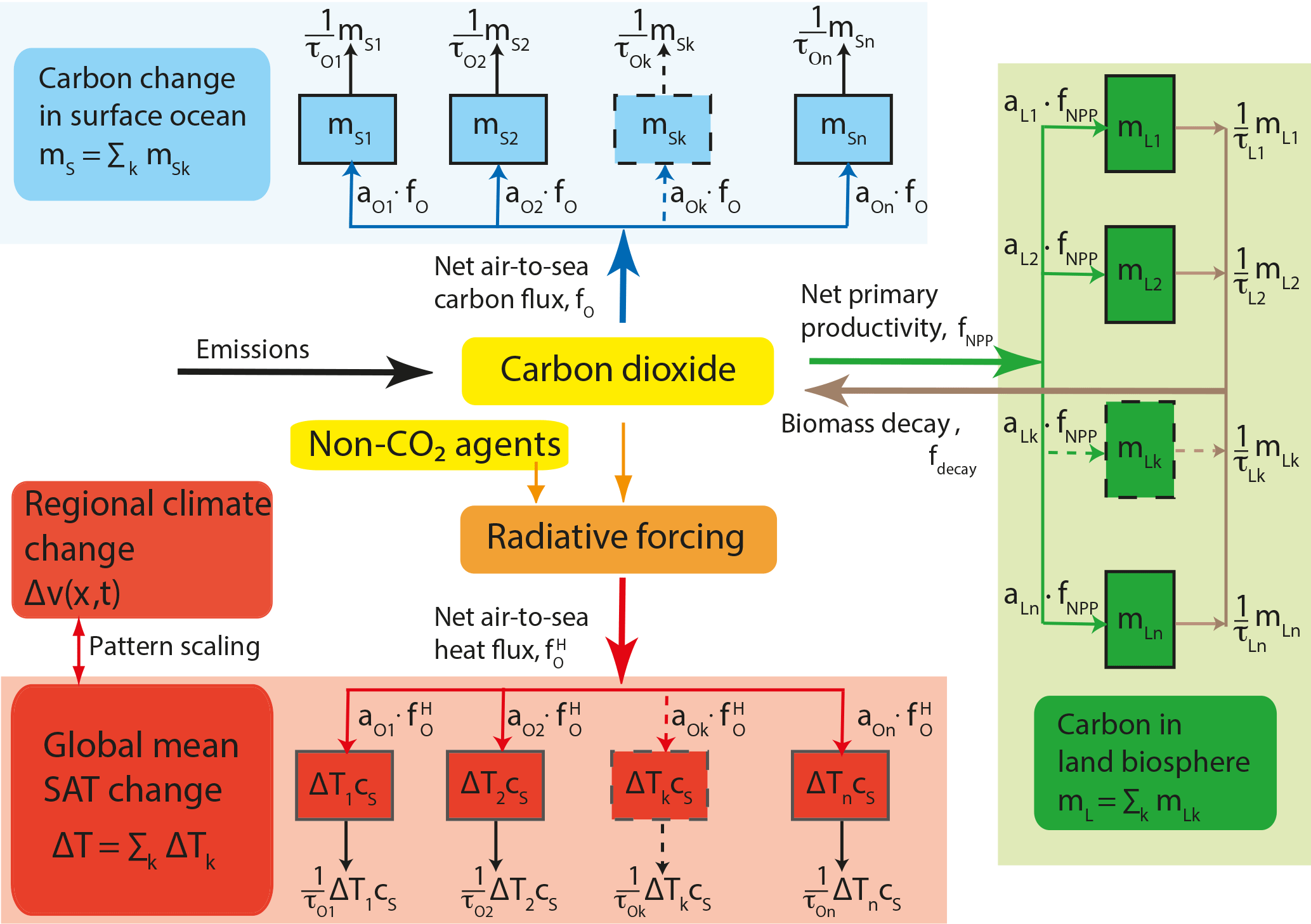
Figure 1BernSCM as a box-type model of the carbon cycle–climate system based on impulse response functions. Heat and carbon taken up by the mixed ocean surface layer and the land biosphere, respectively, is allocated to a series of boxes with characteristic timescales for surface-to-deep ocean transport (τO) and of terrestrial carbon overturning (τL). The total perturbations in land and surface ocean carbon inventory and in surface temperature are the sums over the corresponding individual perturbations in each box (). Using pattern scaling, the response in SAT can be translated to regional climate change for fields v(x,t) of variables such as SAT or precipitation.
An important application of SCMs is in integrated assessment models (IAMs). IAMs are interdisciplinary models that couple a climate component with an energy-economy model to simulate emissions and their climate consequences. Another application of simple models (e.g., Boucher and Reddy, 2008; Bruckner et al., 2003; Enting et al., 1994; Good et al., 2011; Hooss et al., 2001; Huntingford et al., 2010; Joos and Bruno, 1996; Oeschger et al., 1975; Raupach, 2013; Siegenthaler and Oeschger, 1984; Smith et al., 2017; Tanaka et al., 2007; Urban and Keller, 2010; Wigley and Raper, 1992) is to compare, analyze, or emulate more complex models (Geoffroy et al., 2012a, b; Meinshausen et al., 2011; Raper et al., 2001; Thompson and Randerson, 1999). Simple models also play a significant role in previous assessments of the Intergovernmental Panel on Climate Change (e.g., Harvey et al., 1997). The comprehensive scope and interdisciplinarity of such models raise the challenge of maintaining a high and balanced scientific standard across all model components, especially when human resources are limited. This may apply particularly to the climate component, as IAMs are mostly used within the economic and engineering disciplines. Climate and carbon cycle representation are central parts of an IAM and have been critically assessed in the literature (Joos et al., 1999a; Schultz and Kasting, 1997; van Vuuren et al., 2011).
BernSCM is a zero-dimensional global carbon cycle–climate model built around impulse-response representations of the ocean and land compartments, as described previously in Joos et al. (1996) and Meyer et al. (1999). The linear response of more complex ocean and land biosphere models with detailed process descriptions is captured using impulse-response functions (IRFs). These IRF-based substitute models are combined with nonlinear parametrizations of carbon uptake by the surface ocean and the terrestrial biosphere as a function of atmospheric CO2 concentration and global mean surface temperature. Pulse response models have been shown to accurately emulate spatially resolved, complex models (Joos et al., 1996; Joos and Bruno, 1996; Meyer et al., 1999; Joos et al., 2001; Hooss et al., 2001).
BernSCM (Fig. 1) is designed to compute decadal- to millennial-scale perturbations in atmospheric CO2, in climate and in fluxes of carbon and heat relative to a reference state, typically preindustrial conditions. The uptake of excess, anthropogenic carbon from the atmosphere is described as a purely physicochemical process (Prentice et al., 2001). As in pioneering modeling approaches with box-type (Oeschger et al., 1975; Revelle and Suess, 1957) and general ocean circulation models (Maier-Reimer and Hasselmann, 1987; Sarmiento et al., 1992), modification of the natural carbon cycle through potential changes in circulation and the marine biological cycle (Heinze et al., 2015) are not explicitly considered. While such modifications and their potential socioeconomic consequences are vividly discussed in the literature (Gattuso et al., 2015), associated climate–CO2 feedbacks are likely of secondary importance. Estimated uncertainties in the marine carbon uptake due to climate change, including warming-driven changes in CO2 solubility, are found to be smaller in magnitude than uncertainties arising from imperfect knowledge of surface-to-deep physical transport (see Fig. 2d and e in Friedlingstein et al., 2006). The exchange of CO2 between the atmosphere and the surface ocean is described by two-way fluxes, from the atmosphere to the surface ocean and vice versa, and the net flux of CO2 into the ocean is proportional to the air–sea partial pressure difference. CO2 reacts with water to form carbon and bicarbonate ions (Dickson et al., 2007; Orr et al., 2015), and acid–base equilibria are described here using the well-established Revelle factor formalism (Siegenthaler and Joos, 1992; Zeebe and Wolf-Gladrow, 2001). The first-order climate–carbon feedback of a decreasing solubility in warming water is considered. Surface-to-deep exchange, the rate limiting step of ocean carbon and heat uptake, is described using an IRF. On timescales of up to a few millennia, processes associated with ocean sediments and weathering can be neglected. In such a closed ocean–atmosphere–land biosphere system, excess CO2 is partitioned between the ocean and the atmosphere and a substantial fraction of the emitted CO2 remains in the atmosphere and in the surface ocean in a new equilibrium (Joos et al., 2013). This corresponds to a constant term (infinitely long removal timescale) in the IRF representing surface-to-deep mixing. On multimillennial timescales, excess anthropogenic CO2 is removed from the ocean–atmosphere–land system by ocean–sediment interactions and changes in the weathering cycle (Archer et al., 1999; Lord et al., 2016), and the IRF is readily adjusted to account for these processes, important for simulations extending over many millennia.
BernSCM simulates global mean surface temperature and the heat uptake by the planet. The latter is equivalent to the net top-of-the-atmosphere energy flux. Changes in the Earth's heat storage in response to anthropogenic forcing are dominated by warming of the surface ocean and the interior ocean (T. F. Stocker et al., 2013) due to their large heat capacity in comparison with that of the atmosphere and their large thermal conductivity in comparison to that of the land surface. Consequently, the atmospheric and land surface heat capacity is formally lumped with the heat capacity of the surface ocean in the BernSCM. The uptake of heat by the ocean (or planet) is, as for carbon, formulated as a two-way exchange flux. The flux of heat from the atmosphere into the surface ocean is taken to be proportional to the radiative forcing resulting from changes in CO2 and other agents (Etminan et al., 2016). The upward loss of heat from the surface is proportional to the product of the simulated surface temperature perturbation and the (prescribed) climate sensitivity λ (Siegenthaler and Oeschger, 1984; Winton et al., 2010).
As with carbon, surface-to-deep transport is the rate-limiting step for ocean heat uptake and thus for the adjustment of surface temperature to radiative forcing. This transport is key to determine the lag between realized warming and equilibrium warming (Frölicher and Paynter, 2015). Again, this transport is described using an IRF. This IRF encapsulates the finite volume of the entire ocean. It also represents the range of transport timescales associated with advection, diffusion, and convection ranging from decades for the ventilation of thermocline to more than a millennium for deep Pacific ventilation as evidenced by transient tracers such as chlorofluorocarbons and radiocarbon (Olsen et al., 2016). The simulated surface ocean temperature perturbation, taken as a measure of global mean surface air temperature (SAT) change, may be combined with spatial patterns of change in temperature, precipitation, or any other variable of interest to compute regionally explicit changes (Hooss et al., 2001; Joos et al., 2001; B. D. Stocker et al., 2013) (Fig. 1).
Non-CO2 radiative forcing may be prescribed, e.g., following estimates from complex climate–chemistry models (Myhre et al., 2013) or from simple emission-driven non-CO2 modules of radiative forcing related to CO2 chemistry (Joos et al., 2001; Smith et al., 2017) and reconstructions of solar and volcanic forcing (Eby et al., 2012; Jungclaus et al., 2017) and considering the forcing efficacy of non-CO2 agents relative to CO2 forcing (Hansen et al., 2005). Climate sensitivity characterizing the response to radiative forcing is a free parameter in BernSCM. Climate sensitivity may change under increasing warming, particularly in high-emission scenarios (Geoffroy et al., 2012a; Gregory et al., 2015; Pfister and Stocker, 2017). Here, climate sensitivity is assumed to be time invariant and a potential state dependency of climate sensitivity is not considered. This may be changed when more solid information on state dependency becomes available or for the purpose of sensitivity analyses. Similarly, ocean heat uptake efficacy (Winton et al., 2010), influencing the atmospheric temperature response to ocean heat uptake forcing, is set to 1 here.
The present version 1.0 of BernSCM is fundamentally analogous to the Bern model as used already in the IPCC Second Assessment Report, Bern-SAR (whereas different versions of the Bern model family were used in the more recent IPCC reports). BernSCM represents the relevant processes more completely than Bern-SAR, thanks to additional alternative representations of the land and ocean components, which contain a more complete set of relevant sensitivities to temperature and atmospheric CO2.
Here, BernSCM model simulations are compared to previous multimodel studies. The model is run for an idealized atmospheric pulse CO2 emission experiment of Joos et al. (2013), for an idealized CO2 forcing experiment similar to simulations from the Climate Model Intercomparison Project 5 (CMIP5), and for the SRES A2 emission scenario used in the C4MIP study (Friedlingstein et al., 2006).
Together with this publication, BernSCM v1.0 is provided as an open-source Fortran code for free use. The code was also rewritten from scratch, with flexibility and transparency in mind. The model is comprehensively documented, and easily extensible. New alternative model components can be added using the existing ones as a template. A range of numerical solution schemes is implemented. Up to decadal time steps are supported with high accuracy, suitable for the coupling with emission models of coarse time resolution, for example. However, the published code is a ready-to-run stand-alone model, which may also be useful in its own right.
BernSCM offers a physically sound carbon cycle–climate representation, but it is small enough for use in IAMs and other computationally tasking applications. In particular, the support of long time steps is ideally suited to the application of BernSCM as an IAM component, as these complex models often use time steps on the order of 10 years.
BernSCM also offers a tool to realistically assess the climate impact of carbon emissions or emission reductions and sinks, for example in aviation, forestry (Landry et al., 2016), blue carbon management, peat development (Mathijssen et al., 2017), life cycle assessments (Levasseur et al., 2016), or to assess the interaction of climate engineering interventions such as terrestrial carbon dioxide removal with the natural carbon cycle (Heck et al., 2016).
In this paper, we describe the model equations (Sect. 2 and Appendix), illustrative simulations in comparison with previous multimodel studies, and uncertainty assessment (Sect. 3), followed by a discussion (Sect. 4) and conclusions (Sect. 5).
BernSCM simulates the relation among CO2 emissions, atmospheric CO2, radiative forcing (RF), and global mean SAT by budgeting carbon and heat fluxes globally among the atmosphere, the (abiotic) ocean, and the land biosphere compartments. Given CO2 emissions and non-CO2 RF, the model solves for atmospheric CO2 and SAT (e.g., in the examples of Sect. 3), but can also solve for carbon emissions (or residual uptake) when atmospheric CO2 (or SAT and non-CO2 RF) is prescribed, or for RF when SAT is prescribed.
The transport of carbon and heat to the deep ocean, as well as the decay of land carbon, results from complex but linear to first order behavior of the ocean and land compartments. These are represented in BernSCM using IRFs (Green's function). The IRF describes the evolution of a system variable after an initial perturbation, e.g., the pulse-like addition of carbon to a reservoir. It fully captures linear dynamics without representing the underlying physical processes (Joos et al., 1996). More illustratively, the ocean and land models can be considered to consist of systems of uncoupled first-order ordinary differential equations or “box models”, which are an equivalent representation of the IRF model components (Fig. 1).
The net primary production (NPP) of the land biosphere and the surface ocean carbon uptake depend on atmospheric CO2 and surface temperature in a nonlinear way. These essential nonlinearities are described by parametrizations linking the linear model components.
2.1 Carbon cycle component
The budget equation for atmospheric carbon is
where mA denotes the atmospheric carbon stored in CO2, e CO2 emissions, fO the flux to the ocean, mL the land biosphere carbon stock, and t time. Here, mL refers to the (potential) natural biosphere. Human impacts on the land biosphere exchange including land use and land use changes are not simulated in the present version and are treated as exogenous emissions (e). These emissions may be prescribed based on results from spatially explicit terrestrial models. An overview of the model variables and parameters is given in Tables A1 and A2.
The change in land carbon is given by the balance of NPP and decay of assimilated terrestrial carbon,
Decay includes heterotrophic respiration (RH), fire, and other disturbances due to natural processes.
Carbon is taken up by the ocean through the air–sea interface (fO) and distributed to the mixed surface layer (mS) and the deep ocean interior (fdeep):
Global NPP (fNPP) is assumed to be a function of the partial pressure of atmospheric CO2 () and the SAT deviation from preindustrial equilibrium (functions for the implemented land components are given in Appendix A),
The net flux of carbon into the ocean is proportional to the gas transfer velocity (kg) and the CO2 partial pressure difference between surface air and seawater:
where AO is ocean surface area and ε the atmospheric mass of C per mixing ratio of CO2.
The global average perturbation in surface water is a function of dissolved inorganic carbon change (ΔDIC) in the surface ocean at constant alkalinity (Joos et al., 1996) and SAT (Takahashi et al., 1993); ΔDIC and are related to model variables (see Appendix A),
The carbon cycle equation set is closed by the specification of fdecay and fdeep (Sect. 2.3), as well as ΔT, i.e., the coupling to the climate component (Sect. 2.2).
2.2 Climate component
BernSCM simulates the deviation in global mean SAT from the preindustrial state. SAT is approximated by the temperature perturbation of the surface ocean ΔT, which is calculated from heat uptake by the budget equation
where cS is the heat capacity of the surface layer, is ocean heat uptake, and is heat uptake by the deep ocean (and accounts for the bulk of the effective heat capacity of the ocean). Continental heat uptake is neglected due to the much higher heat conductivity of the ocean in comparison to the continent.
is taken to be proportional to RF (Forster et al., 2007) and the deviation of SAT from radiative equilibrium (ΔT=ΔTeq(RF); see Table A2 for parameter definitions),
This relation follows from the assumption that feedbacks are linear in ΔT (e.g., Hansen et al., 1984). ΔTeq is given by
where ΔT2× is climate sensitivity (defined as the equilibrium temperature change corresponding to twice the preindustrial CO2 concentration). Equation (8) describes ocean heat uptake as the difference between RF and the climate system's response, λ⋅ΔT, with the climate sensitivity expressed in .
Climate sensitivity is an external parameter, as the model does not represent the processes determining equilibrium climate response. RF of CO2 is calculated as (Myhre et al., 1998)
where is the preindustrial reference concentration of atmospheric CO2, and RF2× is the RF at twice the preindustrial CO2 concentration. RF of other greenhouse gases (GHGs), aerosols, etc. can be parametrized in similar expressions involving GHG and pollutant emissions and concentrations (Prather et al., 2001). In the provided BernSCM code, non-CO2 RF is treated as an exogenous boundary condition. Total RF is then
The calculation of (Sect. 2.3) completes the climate model.
2.3 Impulse response model components
The response of a time-invariant linear system to a time-dependent forcing f can be expressed by
The function r is the system's IRF, as can be shown by evaluating the integral for a Dirac impulse (). The IRF indicates the fraction remaining in the system at time t of a pulse input at a previous time t′. Because of linearity of the integral, any physically meaningful integrand f can be represented as a sequence of such impulses of varying size.
In BernSCM, an IRF is used to calculate the perturbation of heat and carbon in the mixed surface ocean layer (mixed layer IRF; Joos et al., 1996). For carbon,
and similarly, for heat
This approach has been shown to faithfully reproduce atmospheric CO2 and SAT as simulated with the models from which the IRF is derived (Joos et al., 1996). For temperature, the linear approach works since relatively small and homogeneous perturbations of ocean temperatures do not affect the circulation strongly and can be treated as a passive tracer (Hansen et al., 2010). Note that for compatibility with commonly used units, carbon fluxes are expressed in Gt yr−1, while heat fluxes are expressed in joules per second (watt) in Eqs. (13) and (14), respectively.
Equation (13) closes the ocean C budget equation (Eq. 3), as can be seen by taking the derivative with respect to time (using r(0)=1),
where fdeep is the flux to the deep ocean. Similarly, Eq. (14) closes the heat budget equation (Eq. 7) for the surface ocean,
Another IRF is used for the carbon mL in living or dead biomass reservoirs of the terrestrial biosphere,
Again, Eq. (17) closes the budget equation for the land biosphere (Eq. 2), as shown by the derivative with respect to time,
The time derivative of the land IRF is also known as the decay response function Joos et al. (e.g., 1996).
The IRFs above can be expressed as a sum of exponentials,
where the constant term a∞ corresponds to an infinite decay timescale.
The ocean IRF contains a positive constant coefficient a∞, indicating a fraction of the perturbation that will remain indefinitely (implied by carbon conservation in the ocean model). CaCO3 compensation by sediment dissolution and weathering (Archer et al., 1999) are not considered here, but could be described using analogous elimination processes with timescales on the order of 104 to 105 years (Joos et al., 2004). We emphasize that the implementation considering only the partitioning of excess carbon among atmosphere, land, and ocean (hence a∞≠ 0), neglecting ocean sediment interactions and weathering flux perturbations, is only valid for timescales shorter than about 2000 years. In land biosphere models, in contrast, organic carbon is lost to the atmosphere by oxidation to CO2 at nonzero rates, and consequently all timescales are finite (i.e., a∞=0), and the IRF tends to zero (Fig. 2).
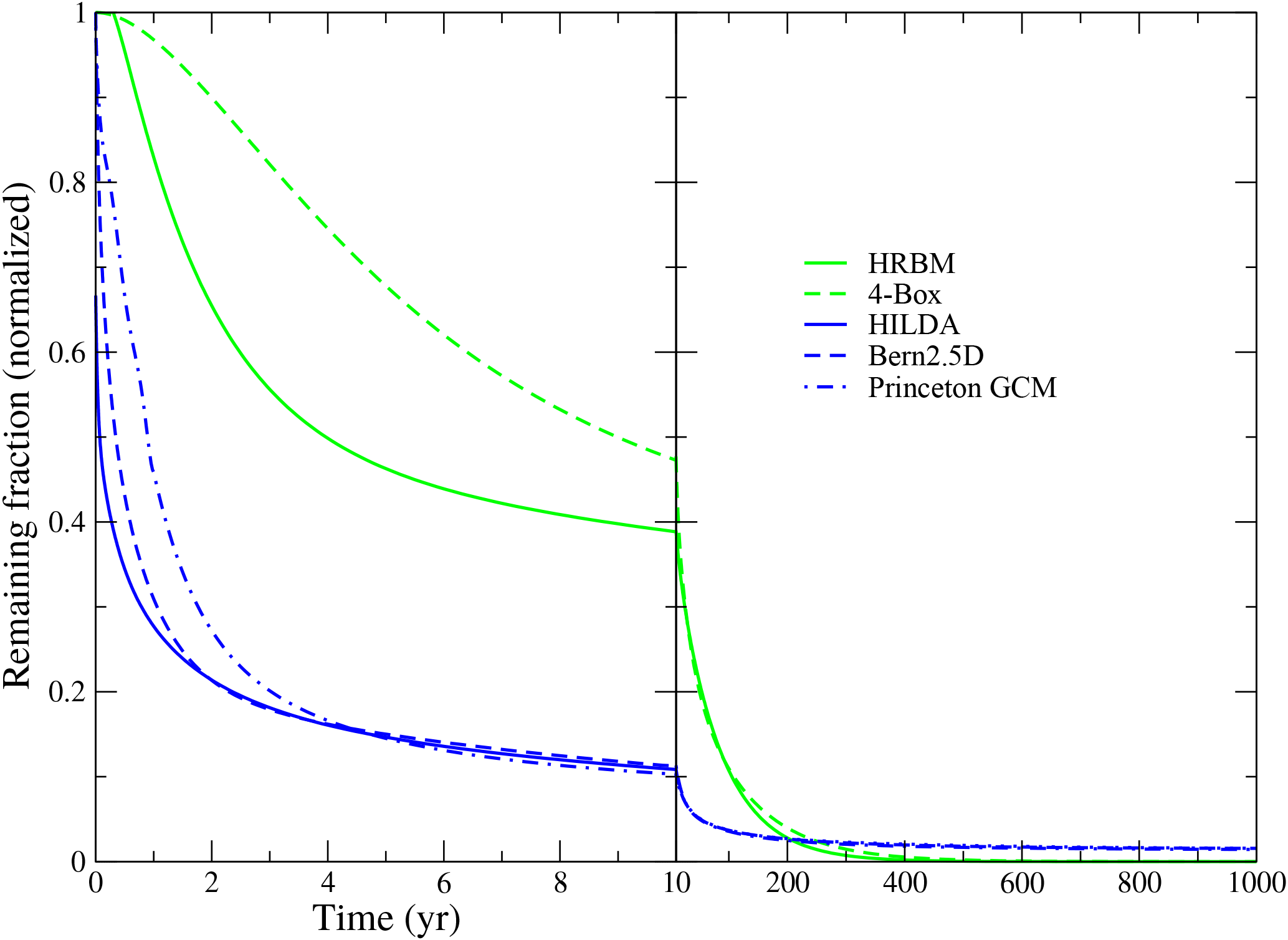
Figure 2IRFs of ocean (blue) and land (green) model components (without temperature dependence). Ocean components are normalized to a common mixed-layer depth of 50 m (multiplied by Hmix∕50 m), causing initial response to deviate from 1.
Inserting the formula (Eq. 19) in the pulse response equation (Eq. 12) yields (f is a perturbation flux when a∞≠ 0)
Thus the expression (Eq. 12) separates into a set of independent integrals mk corresponding to the number of timescales of the response. Taking the time derivative of the expression (Eq. 20) reveals the equivalence to a system of uncoupled first-order ordinary differential equations.
The direct numerical evaluation of Eq. (12) involves integrating over all previous times at each time step. The differential form Eq. (21) allows a recursive solution, which is much more efficient, especially for long simulations (the recursive solution implemented in BernSCM is described in Appendix B).
The differential equation system (Eq. 21) can be considered to consist of several boxes, whereby each box mk receives a fraction ak of the input f and has a characteristic turnover time τk (Fig. 1). In the following this is referred to as a box model. For the mixed ocean surface layer the carbon content of box k is given by
and the change in total carbon content in the mixed layer is
Similar equations describe the heat content in the ocean surface layer, as well as the carbon stored in the land biosphere (Fig. 1).
The timescales of an IRF describing a linear system are equivalent to the inverse eigenvalues of the model matrix of that system and may also be interpreted in the context of the Laplace transformation (Enting, 2007; Raupach, 2013). For example, the timescales of the mixing layer IRF are the inverse eigenvalues of a matrix describing a diffusive multilayer ocean model (Hooss et al., 2001). A large model matrix yields a spectrum of many eigenvalues and timescales and corresponding model boxes. In practice, IRFs are approximated with fewer fitting parameters and, equivalently, timescales (four to six in the case of BernSCM). Joos et al. (1996) used IRFs combined from two or more functions to minimize the number of parameters needed for an accurate representation. In BernSCM, simple IRFs of the form (Eq. 19) are used exclusively. This allows adequate accuracy and a consistent interpretation as a multibox model.
Thinking of IRF components as box models is conceptually meaningful. The simple Bern 4-box biosphere model (Siegenthaler and Joos, 1992), for example, contains boxes corresponding to ground vegetation, wood, detritus, and soil (Appendix A). The High-Resolution Biosphere Model (HRBM) land component (Meyer et al., 1999), however, is abstractly defined by an IRF, but corresponds to boxes which correlate with biospheric reservoirs. However, since different box models may show a similar response, in practice the coefficients ak and timescales τk may not be uniquely defined by the IRF and should be interpreted primarily as abstract fitting parameters (Enting, 2007; Li et al., 2009).
The IRF representation is, strictly speaking, only valid if the described subsystem is linear and the timescales of the system are time invariant. Then, the response function r does not depend on time and on state variables. In the BernSCM, major nonlinearities in the carbon cycle, namely air–sea gas exchange and the nonlinear carbonate chemistry, and changes in NPP in response to changes in environmental conditions are treated by separate nonlinear equations (Eqs. 4 and 5), while surface-to-deep ocean transport of carbon and heat and respiration of carbon in litter and soils are viewed as approximately linear processes using IRFs. However ocean circulation and the respiration of carbon from soil and litter is likely to change under global warming, violating the assumption of linearity. In practice, the IRF representation remains a useful approximation as long as the impact of associated nonlinearities on simulated atmospheric CO2 and temperature remain moderate.
The interpretation of the IRF representation as a box model provides a starting point for considering nonlinearities in the response. To account for nonlinearities, the response timescales τk and the coefficients ak may be gradually adjusted as a function of state variables such as temperature. As the integral form (Eq. 12) involves integration over the whole history at each time step, changing parameters along the way would result in inconsistencies. In contrast, the differential or box model form (Eq. 21) does not depend on previous time steps. Changing the model parameters from one step to the next thus equates to applying a slightly different model at each time step. Within each time step, the parameters remain constant, and the solution for the linear case applies. As time steps are small compared to the whole simulation, this discretization yields accurate results, which is confirmed by the close agreement between the different time resolutions (Table B1).
Varying coefficients have been successfully implemented and tested for the HRBM land component and its decay IRF (Meyer et al., 1999). In this way, the enhancement of biomass decay by global warming is captured (see the Appendix A and Sect. 3.1). In such a modification, the advantage of the IRF and the equivalent box model representation – the faithful representation of the characteristic response timescale of a model system – is largely maintained, while at the same time the impact of time- and state-dependent system responses on simulated outcomes is approximated.
3.1 Model setup for sensitivity analyses and uncertainty assessment
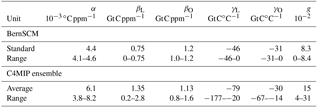
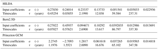
The carbon cycle–climate uncertainty of simulations with BernSCM can be assessed in two ways. First, to assess structural uncertainty, different substitute models for the ocean and land components can be used. Currently, this approach is quite limited by the set of available substitute models (see Appendix A). Second, parameter uncertainty can be assessed by varying the temperature and CO2 sensitivities of the model, based on a standard set of components that represent the key dependencies as completely as possible (here, the IRF substitutes for the high-latitude exchange/interior diffusion–advection (HILDA) ocean model (Joos et al., 1996) and for the HRBM land biosphere model (Meyer et al., 1999) are used in the standard setup).
The uncertainties of the global carbon cycle concern the sensitivity of the modeled fluxes of carbon and heat to changing atmospheric CO2 and climate. Key uncertainties strongly affecting the overall climate response are associated with land C storage: the dependency of NPP on CO2 (CO2 fertilization), and the dependency of land C on temperature (fdecay increases with warming). This gives rise to large and opposed carbon flux perturbations which are both very uncertain in magnitude (Le Quéré et al., 2016). While all substitute land models available for BernSCM include CO2 fertilization, only the HRBM substitute model represents temperature sensitivity of biomass decay (Appendix A2).
As for the ocean, the uncertainty of heat uptake into the surface ocean is treated in terms of climate sensitivity (Eq. 8). The efficiency of the uptake of heat () and carbon (fdeep) into the deep ocean is not sensitive to temperature, as the currently available substitute models all represent a fixed circulation pattern (IRF or box model parameters are not temperature dependent; Appendix A1). The nonlinear chemistry of CO2 dissolution in the surface ocean (Eq. 4), which determines the sensitivity of ocean C uptake to atmospheric CO2, is scientifically well established (Dickson et al., 2007; Orr and Epitalon, 2015) and is not treated as an uncertainty in BernSCM. The temperature sensitivities of NPP and CO2 dissolution in the surface ocean are treated as uncertain here, but have secondary influence on the climate response.
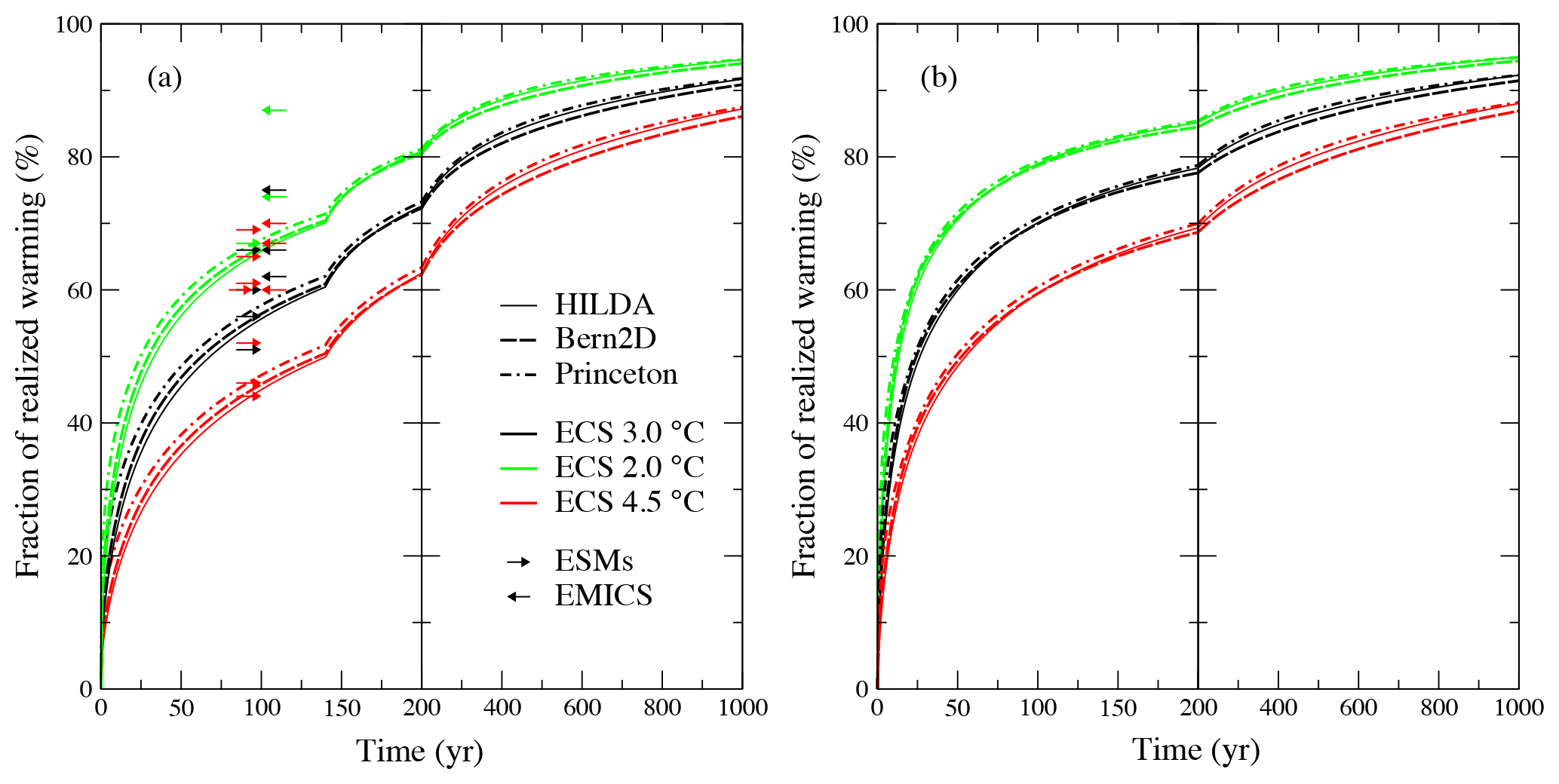
Figure 3Fraction of realized warming (temperature divided by the equilibrium temperature for the current RF) for idealized experiments with prescribed atmospheric CO2 concentration increase from preindustrial levels; panel (a) shows an exponential CO2 increase by 1 % yr−1 over 140 years to approximately 4 times the preindustrial concentration (and linear increase in RF); panel (b) shows an abrupt increase to 4-fold CO2 concentration. BernSCM simulations are shown for climate sensitivities of 2, 3, and 4.5 K and the three available ocean model substitutes as indicated in the legend. Arrows in panel (a) indicate the corresponding warming fractions at year 99 compiled by Frölicher and Paynter (2015, Tables 1, 2 in their Supplement) for Earth system models (ESMs, right-pointing) and Earth system Models of Intermediate Complexity (EMICs, left-pointing); arrow colors indicate climate sensitivities below 2.5 K (green), between 2.5 and 3.5 K (black), and above 3.5 K (red).
Similar to previous studies using models from the Bern family (Plattner et al., 2008; Joos et al., 2001; Meehl et al., 2007; Van Vuuren et al., 2008), the parameter uncertainty range is assessed using the following setups.
- Coupled.
-
All temperature and CO2 sensitivities are set to their standard values.
- Uncoupled.
-
All sensitivities are set to zero (except for the ocean CO2 dissolution chemistry).
- C-only.
-
Only CO2 dependencies are considered (CO2 fertilization).
- T-only.
-
Only temperature dependencies are considered in the land module (NPP, decay).
We performed simulations with these different setups. In Sect. 4.2, we probe the timescales of the temperature response in simulations in which atmospheric CO2 is abruptly (instantaneously) quadrupled or by increasing CO2 radiative forcing linearly within 140 years. In Sect. 4.3, we probe the response of the coupled system to a pulse-like release of 100 Gt C into the atmosphere. Finally in Sect. 4.4, we analyze carbon cycle–climate feedbacks relying on simulations over the industrial period and for the SRES A2 scenario. BernSCM results are compared with the results from three multimodel intercomparison projects: the Climate Model Intercomparison Project 5 (CMIP5) with results as summarized by Frölicher and Paynter (2015), an analysis of carbon dioxide and climate impulse response functions (Joos et al., 2013, here referred to as IRFMIP), and the C4MIP climate–carbon cycle feedback analysis (Friedlingstein et al., 2006).
3.2 Fraction of realized warming and idealized forcing experiments
The climate response of BernSCM is illustrated using idealized simulations with prescribed forcing. One series of simulations (a) was run for CO2 concentration increasing exponentially from the preindustrial value by 1 % yr−1 over 140 years to approximately 4 times the preindustrial concentration, corresponding to a linear increase in RF (Fig. 3a); in a second series of simulations (b), CO2 was abruptly increased to 4 times the preindustrial concentration (Fig. 3b).
Frölicher and Paynter (2015) compare similar simulations of Earth system models (ESMs) performed within the Coupled Model Intercomparison Project Phase 5 (CMIP5), and Earth System Models of Intermediate Complexity (EMICs) (Joos et al., 2013). As a model comparison metric sensitive to the long-term climate response, Frölicher and Paynter (2015) use the fraction of realized warming, defined by the ratio of the temperature response at a given year and the equilibrium temperature for the corresponding RF. They show that the smaller realized warming of ESMs in comparison to EMICs (Fig. 3) is connected to a higher long-term warming response; this implies an increase in the coefficient relating global warming to cumulative carbon emissions on multicentennial timescales and suggests a lower quota on allowed emissions for a given global warming target (Frölicher and Paynter, 2015). The realized warming fraction simulated with BernSCM is in good agreement with the responses of the ESMs (and lower on average than that of the EMICs). The validity of the IRF approach has also been shown by Good et al. (2011) using a SCM to reconstruct and interpret atmosphere–ocean general circulation model (AOGCM) projections. For the 150-year timescale of the CMIP5 experiments, Geoffroy et al. (2012a, b) show that the climate response of AOGCMs is well captured by a two-layer energy balance model with two effective response timescales.
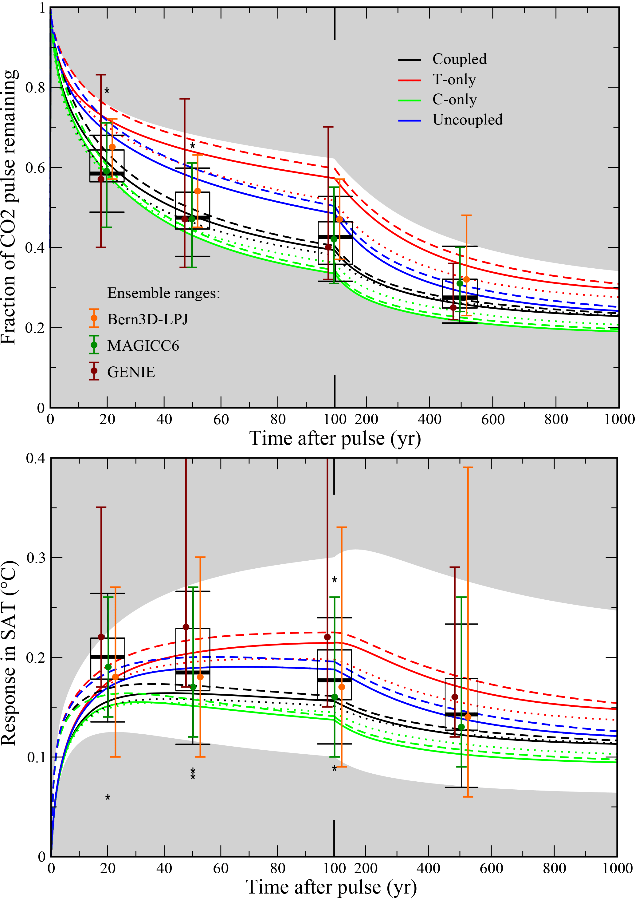
Figure 4IRFMIP pulse response range compared to BernSCM range for parameter uncertainty (colors according to legend) and structural uncertainty, with model versions HILDA–HRBM (solid lines), HILDA–4-box (dots), and Princeton–HRBM (dashed). Standard climate sensitivity is 3 ∘C, and a climate sensitivity range of 2–4.5 ∘C is shown by the white area (envelope of all BernSCM runs). Single-model ensemble ranges from IRFMIP are included as error bars indicating the 5–95 % range and dots indicating the median. The multimodel IRFMIP range is shown by box plots indicating median (bold black line), first quartiles (box), and extreme values (whiskers) excluding outliers deviating from the median by more than 1.2 times the interquartile distance (asterisks).
In BernSCM, the fraction of realized warming depends primarily on the choice of climate sensitivity and is qualitatively similar for the different model setups. Such a clear relationship is not seen in the EMS and EMICs. Thus the structural uncertainty and model differences of complex models are not fully represented in BernSCM. The BernSCM climate response to abrupt warming (Fig. 3b) is qualitatively similar, especially on multicentennial timescales.
3.3 Impulse response experiment
Coupled carbon cycle–climate models can be characterized and compared based on their response to a CO2 emission pulse to the atmosphere (Joos et al., 2013). The airborne fraction (AF) denotes the fraction of emissions found in the atmosphere at a given time. In IRFMIP, the AF for a pulse of 100 Gt C, emitted on top of current (i.e., year 2010) atmospheric CO2 concentrations, was simulated by a set of 15 carbon cycle–climate models of different complexity. For three of these models (Bern3D-LPJ, GENIE, MAGICC), ensembles sampling the parameter uncertainty of these models are included in IRFMIP. Thus, IRFMIP captures structural as well as parameter uncertainty.
The IRFMIP pulse experiment was repeated with BernSCM, exploring parameter uncertainty of the carbon cycle (Sect. 3.1), as well as structural uncertainty, using the ocean model IRFs HILDA and Princeton (Sarmiento et al., 1992) in various combinations with the land biosphere components HRBM and the Bern 4-box model (Fig. 4). Simulations were run for equilibrium climate sensitivities of 3 (standard setup), 2, and 4.5 ∘C.
The AF simulated with BernSCM broadly agrees with the set of simulations from IRFMIP. At 100 years after the pulse, the AF is 0.40 (0.34–0.57) for a climate sensitivity of 3 ∘C (for coupled setup with uncertainty range in brackets). Climate sensitivity uncertainty only slightly affects the upper end of this range (Fig. 4). For AF simulated with BernSCM, the standard coupled setup is close to the IRFMIP multimodel median. The BernSCM uncertainty range is asymmetric, like the IRFMIP multimodel range. For the MAGICC and GENIE ensembles, the medians also correspond with the BernSCM standard case, while the uncertainty ranges are more symmetric.
The BernSCM SAT response also broadly agrees with IRFMIP. The standard coupled simulation is somewhat lower than the IRFMIP median, which is explained in part by the climate sensitivity (3 ∘C) being slightly lower than the IRFMIP average (3.2 ∘C). The short-term temperature response of BernSCM in particular is on the lower side of the IRFMIP range, suggesting stronger ocean mixing. The quickest initial temperature increase in the BernSCM simulations is obtained with the Princeton ocean model component (dashed lines), which shows a slower initial mixing to the deep ocean than the other implemented components (Fig. 2). The comparability of the SAT projections is limited, as the range of climate sensitivities considered in the BernSCM simulations (2–4.5 ∘C) differ somewhat from those of the IRFMIP multimodel set (1.5–4.6 ∘C) and the single model ensembles (1.9–5.7 ∘C) and are compounded with RF differences resulting from the uncertainty in atmospheric CO2.

Figure 5Land, ocean, and airborne fractions of the 100 Gt C CO2 pulse shown in Fig. 4 for the coupled (solid lines and colored areas), T-only (dashed), C-only (dotted), and uncoupled (dash-dotted) model setups. In the T-only case, the land biosphere exhibits a net release (light green shading), and the ocean uptake consists of the sum of this area and the area delimited by the dashed line below the line at 1; for the uncoupled case, land uptake is zero and ocean uptake extends from the dashed–dotted line to unity.
Figure 5 shows how the added carbon is redistributed within the Earth system. In the coupled setup, the fraction of the initial pulse sequestered by the land and by the ocean increases over the first century, while the airborne fraction decreases. After 100 years, slightly more than 20 % of the added carbon is stored in the land and about 40 % in the ocean. The ocean continues to sequester excess carbon in the following centuries to become the dominant sink for excess carbon. In contrast, the land returns part of the sequestered carbon back to the atmosphere and ocean as decreasing atmospheric CO2 reduces the modeled CO2 fertilization of the land biosphere. In the T-only setup, in which CO2 fertilization is not operating, the land is a source of carbon to the atmosphere due to accelerated soil turnover in response to warming. The largest land sink is simulated in the C-only setup, in which soil turnover timescales remain invariant and CO2 fertilization is on. The different BernSCM setups span a range of plausible land biosphere and ocean responses to continued anthropogenic CO2 emissions as reflected in the simulated range in the airborne fraction (Figs. 4a and 5).
3.4 Carbon cycle–climate feedbacks
Climate models with explicit and detailed carbon cycle components exhibit a wide range of responses, as shown in the intercomparison studies of climate models with a detailed carbon cycle, C4MIP (Friedlingstein et al., 2006) and CMIP5 (Jones et al., 2013). The authors analyzed the feedback of carbon cycle–climate models using linearized sensitivity measures. These are derived from a simulation with temperature dependence (“coupled”) and one without (“uncoupled”; note that these names have a different meaning in BernSCM). Total CO2 emissions for the coupled (left-hand side) and uncoupled (right-hand side) simulations can be expressed as
where ΔCA is the cumulative change in atmospheric CO2 (in parts per million) in the coupled (c) or uncoupled (u) cases, and the terms in parentheses represent the total sensitivity of C storage to ΔCA; in particular, β is the sensitivity of carbon storage to atmospheric CO2 (in Gt C ppm−1) on land (βL) or in the ocean (βO). γ is similarly the sensitivity in carbon storage to climate change, and α is the linear transient climate sensitivity to CO2 (∘C ppm−1) as in Friedlingstein et al. (2006); ε converts ppm to Gt C (see Table A2; the formula in the original paper implies identical units for atmospheric and stored carbon).
The climate–carbon cycle feedback is measured by the feedback metric g, defined by
and is thus estimated by
Thus the feedback strength scales with the assumed climate sensitivity and the temperature sensitivities and is reduced by CO2-induced sinks.
The C4MIP study used a SRES A2 emission scenario to compare the carbon cycle sensitivities of a range of models. As in the C4MIP exercise, BernSCM was run for SRES A2 without any non-CO2 forcings (Fig. 6; prescribed historical and scenario emissions were smoothed with the R smooth.spline function (R Core Team, 2015) for 41 degrees of freedom for use with different time steps). Land use was treated as an exogenous CO2 emission, while the land model simulates an undisturbed biosphere.
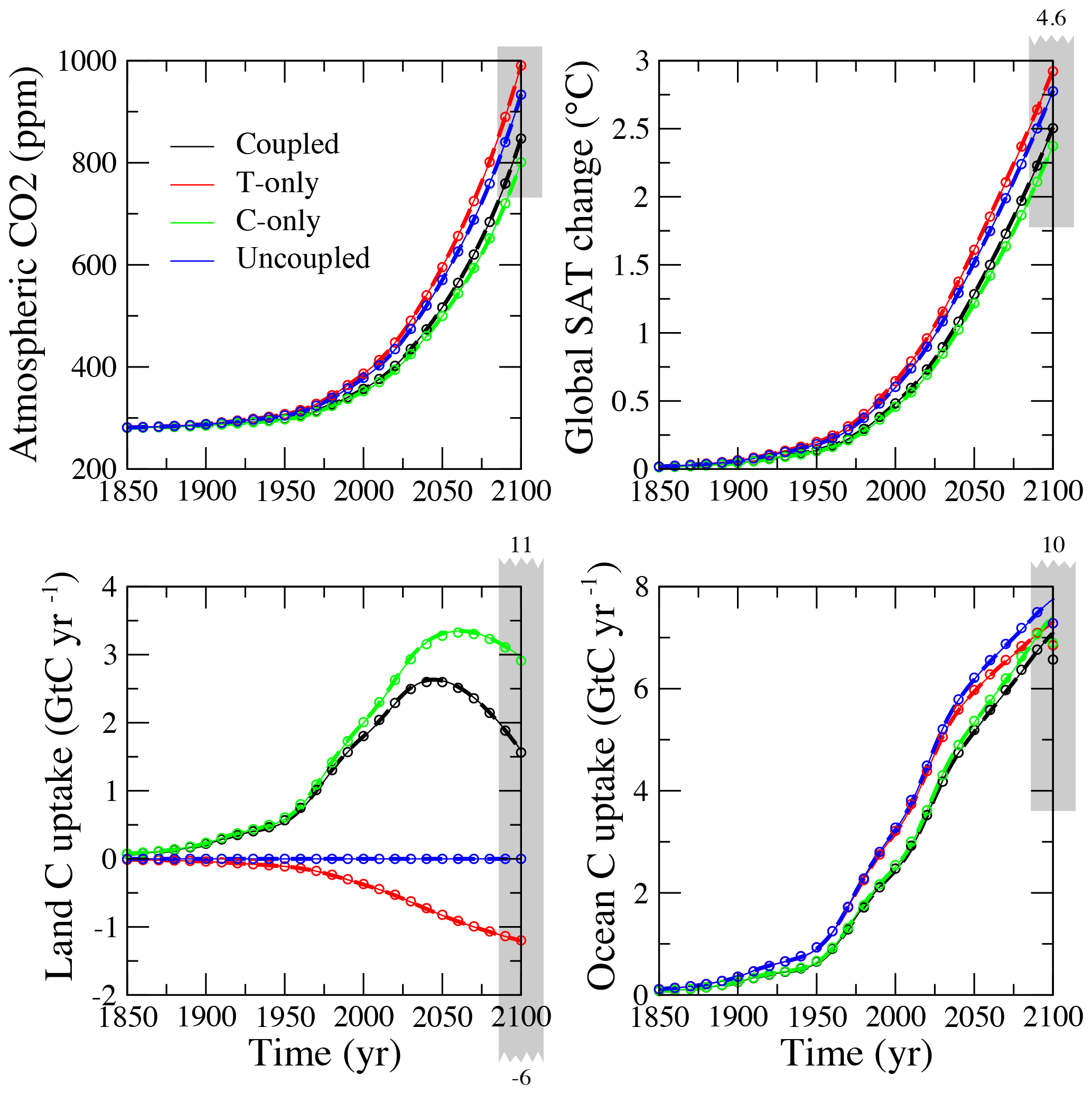
Figure 6BernSCM simulations of the SRES A2 scenario used for C4MIP, with a climate sensitivity of 2.5 ∘C and the HILDA–HRBM ocean–land components. Results for three numerical schemes are overlaid; (i) 0.1-year Euler forward time step (solid thin line), (ii) 1-year implicit time step (dashed bold line), (iii) 10-year implicit time step with piecewise linear approximation of fluxes (circles); the difference at this resolution is only visible in the C uptake. The C4MIP model range at 2100 is indicated by grey bars; numbers above or below the bars indicate values outside of the chart range.
The BernSCM sensitivity setups can be expressed in terms of the C4MIP sensitivity metrics: T-only corresponds to βL=0, C-only to , and uncoupled to . This can be used to estimate climate–carbon cycle feedback g captured in BernSCM. The sensitivity metrics for the BernSCM standard simulation (HILDA-HRBM with coupled carbon cycle) lie within the C4MIP range (Table 1). The uncertainty range for BernSCM, however, is not congruent with the multimodel range of C4MIP. Maximum and standard sensitivity for BernSCM are practically identical. Notably, this sensitivity is smaller (absolutely) than the C4MIP average for the land carbon response to CO2 increase and warming. The resulting gain g is also smaller, though this results in large part from the lower climate sensitivity in BernSCM (which corresponds to 2.5 ∘C as used for the Bern-CC model contribution to C4MIP). The lower end (in absolute terms) of the BernSCM carbon cycle sensitivity range is, however, zero per definition for all but the ocean-CO2 sensitivity βO (see Sect. 3.1). As a consequence, the climate–carbon cycle feedback range also includes zero. In contrast, the C4MIP range does not include zero for all sensitivity parameters.
The land carbon uptake until 2100, under the different BernSCM configurations, varies over 500 Gt C (Fig. 6), more than 3 times the range of ocean uptake (180 Gt C). This partly reflects the limited coverage of the uncertainty in ocean mixing but also the fact that the land carbon sink is, together with the source related to land use, the most uncertain item in the budget (Le Quéré et al., 2009).
We simulated illustrative scenarios from two recent multimodel studies, C4MIP and IRFMIP, to compare BernSCM to the literature of carbon cycle–climate models. The results show that BernSCM is broadly representative of the current understanding of the global carbon cycle–climate response to anthropogenic forcing (in a time-averaged sense that does not address internal variability). The BernSCM uncertainty range in CO2 and SAT projections is broadly similar to the ranges spanned by probabilistic single-model ensembles and multimodel “ensembles of opportunity” such as the 15 IRFMIP models. The BernSCM uncertainty range shown consists mainly of parameter uncertainty and to a small extent of structural uncertainty. For the standard coupled model setup, the sensitivities of ocean and land carbon uptake to changing CO2 and climate (Table 1) of BernSCM are within the range of the detailed carbon cycle models in C4MIP. However, as some C4MIP models show much higher sensitivities, the BernSCM range does not capture the full C4MIP multimodel range. However, the C4MIP set is unlikely to sample uncertainty exhaustively, as each model contributed only a single, most likely simulation. Thus it does not include zero (or weak) sensitivities, whereas the BernSCM range does.
As Fig. 6 shows, solutions with different time steps and numerical schemes as implemented in BernSCM are largely equivalent for a sufficiently smooth forcing. This offers the flexibility to opt for simplicity of implementation or maximum speed as required by the application (see also Appendix B).
BernSCM does not explicitly distinguish between surface atmosphere and surface ocean temperature to compute global mean SAT perturbation. This is in contrast to some energy balance calculations used to analyze results from state-of-the-art ESMs (e.g., Geoffroy et al., 2012b). The BernSCM approach follows earlier work of Siegenthaler and Oeschger (1984). It is further guided by the similarity in reconstructions of marine nighttime air and sea surface temperature perturbations (T. F. Stocker et al., 2013) that are consistent with the short, monthly relaxation timescale for air–sea heat exchange. The focus of the BernSCM is on the representation of the transport of heat from the surface into the thermocline and the deep ocean on decadal to multicentury timescales, while information on seasonal and spatial changes such as on land–sea air temperature differences or polar amplification may be obtained by applying suitable spatial perturbation patterns as derived from state-of-the-art models.
Table 1C4MIP sensitivity metrics. The BernSCM range covers the carbon cycle settings as discussed in Sect. 3.1, and different combinations of model components (HILDA–HRBM, HILDA–4-box, Princeton–HRBM); the C4MIP range covers all participating models.
Currently, a limited set of substitute models is available and included with BernSCM. The simple structure and open-source policy of BernSCM allows users to address these current limitations according to the needs of their applications. More components can be added using the existing ones as a template. This requires the specification of the IRF and the parametrization of gas exchange for the surface ocean or NPP for the land biosphere (as described in Joos et al., 1996; Meyer et al., 1999).
Ocean transport is known to vary under climate change with some consequences for heat and carbon uptake (Joos et al., 1999b). Here, we applied time-invariant ocean transport parameters (, ). It is in principle possible to represent temperature dependency of ocean transport in a similar way as it is performed for the climate dependency of heterotrophic respiration for the HRBM land biosphere substitute model (Meyer et al., 1999). In the current BernSCM version, the same IRF parameters are applied for the transport of carbon and heat from the surface ocean to the interior ocean. Thereby, it is implicitly assumed that the spatial pattern of change is the same for temperature and carbon. This appears to be a reasonable first-order approximation on decadal to century timescales as perturbations in temperature and carbon show similar patterns with decreasing perturbations from the surface to depth. In future efforts, one may differentiate the ocean IRF for heat and carbon, in particular when more information from long-term multicentury to millennial-scale ESM simulations becomes available. The application of the same IRF for carbon and heat in individual model runs implies that modeled carbon and heat transport tend to be physically consistent. In contrast, some other simple models employ different transport parameters for heat and carbon and varied these parameters independently in probabilistic studies.
A distribution of timescales applies to ocean transport processes as evidenced by observations of transient and time-dependent tracers such as chlorofluorocarbons and bomb-produced and natural radiocarbon and biogeochemical tracers (Key et al., 2004; Olsen et al., 2016). This continuum is sometimes approximated by one timescale, also termed heat uptake efficiency (e.g., Gregory et al., 2009), and by two timescales, as in Geoffroy et al. (2012b). The one-to-two timescale approximations were used to analyze relatively short ESM simulations that do not yet reveal the multicentury response timescales of the deep ocean. We note that the equivalent ocean depth of the simple energy balance model of Geoffroy et al. (2012b) for their AOGCM ensemble is only 1182 m compared to a mean ocean depth of about 3800 m. The ocean IRFs used in the BernSCM are derived from long simulations with ocean-only or simplified models. The range of distinct timescales used to construct the IRF faithfully approximates the sub-annual to multicentury response continuum of the parent models as shown in earlier work (Joos et al., 1996). Further, the BernSCM IRF model represents the heat capacity of the entire ocean.
The BernSCM model may be extended to model perturbation in the signatures and exchange fluxes of the carbon isotopes 13C and 14C as demonstrated in earlier work (Joos et al., 1996). This was not implemented here to keep the code as simple as possible and as most potential users are likely concerned with the evolution of climate and atmospheric CO2 .
A potential future application of BernSCM is to use it as an emulator of the global long-term response of complex climate–carbon cycle models by adding the corresponding substitute model components. Additionally, pattern scaling can be applied to transfer the global mean temperature signal into spatially resolved changes in surface temperature, precipitation, cloud cover, etc., exploiting the correlation of global SAT with regional and local changes (Hooss et al., 2001). This allows us to drive spatially explicit models, e.g., of terrestrial vegetation Joos et al. (as in 2001); Strassmann et al. (as in 2008) or impacts related to climate change (e.g., as in Hijioka et al., 2009). Patterns of change are generally similar across models for temperature, whereas patterns in precipitation are more uncertain and show greater variability among models (Knutti and Sedlacek, 2013) and are forcing dependent (Shine et al., 2015). We also note that natural variability strongly influences the space-time evolution of climate change (Deser et al., 2012). Patterns may be scaled with changes in global mean SAT as indicated in Fig. 1 or dependencies on radiative forcing may be considered (Shine et al., 2015)
The addition of further alternative model components will extend the structural uncertainty that can be represented with BernSCM. A sufficient coverage of structural uncertainty could allow the interpolation among alternative model components to represent uncertainty with scalable parameters (and removing the distinction between structural and parameter uncertainty). Such a parametrization of the uncertainty would enhance the possibilities for probabilistic applications of BernSCM, although more sophisticated models are available for observation-constrained probabilistic quantification of climate targets (Holden et al., 2010; Steinacher and Joos, 2016; Steinacher et al., 2013).
BernSCM is a reduced-form carbon cycle–climate model that captures the characteristics of the natural carbon cycle and the climate system essential for simulating the global long-term response to anthropogenic forcing. Simulated atmospheric CO2 concentrations and SATs are in good agreement with results from two comprehensive multimodel ensembles. Process detail is minimal, due to the use of IRFs for system compartments that can be described linearly and nonlinear parametrizations governing the carbon fluxes into these compartments. This framework allows, in particular, the representation of the wide range of response timescales of the ocean and land biosphere and the nonlinear chemistry of CO2 uptake in the surface ocean – both essential for reliably simulating the global climate response to arbitrary forcing scenarios.
Due to its structural simplicity and computational efficiency, BernSCM has many potential applications. In combination with pattern scaling, BernSCM can be used to project spatial fields of impact-relevant variables for applications such as climate change impact assessment, coupling with spatially explicit land biosphere models, etc. With alternative numerical solutions of varying complexity and stability to choose from, applications range from educational to computationally intensive integrated assessment modeling. BernSCM also offers a model-based alternative to global warming potentials for estimation of the climate impact of emissions and can be used to quantify climate benefits of mitigation options by applying emissions- or concentration-driven simulations.
The generic implementation of linear IRF components offers a transparent, extensible climate model framework. Current limitations concern the number of available substitute models (limiting the uncertainty range represented), and ocean transport not influenced by climate change. An addition of further alternative model components and more flexible representation of sensitivities in terms of continuously variable parameters would further increase the models' usefulness, for example for probabilistic applications.
The source code of the Bern Simple Climate Model is available from the GitHub repository at https://doi.org/10.5281/zenodo.1038117.
A1 Ocean
Currently available ocean components include substitute models for the high-latitude exchange/interior diffusion–advection model (HILDA Joos et al., 1996), Bern2D (Stocker et al., 1992), and the Princeton general circulation model (GCM) (Sarmiento et al., 1992). Ocean model parameters of the equations described in the main text are listed in Table A3 for the mixed-layer IRF/box models and in Table A2 for other equations. The IRF/box model parameters given here are recalculated by fitting a sum of six exponential functions and one constant to the original response functions as given in Joos and Bruno (1996). The original functions treated the first few years separately; the approximation to a purely exponential form simplifies the equations and has a negligible effect on accuracy. The parametrization of ocean surface CO2 pressure is the same for all available ocean components and is given below.
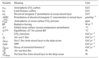
Table A2Model parameters.
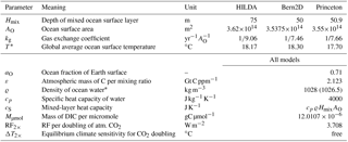
* The first value is used in the climate component equations, the value in parentheses in the C cycle component equations.
Ocean surface CO2 pressure perturbations are fitted as a function of the globally averaged unperturbed surface temperature T* and perturbations in dissolved inorganic carbon (DIC) by Joos et al. (1996) using carbonate chemistry coefficients summarized by Millero (1995):
The expression holds for unperturbed global average surface water temperature T* between 17.7 and 18.3 ∘C and for between 0 and 1320 ppm.
Ocean surface CO2 pressure for global surface temperature perturbation ΔT (Takahashi et al., 1993):
A2 Land biosphere
Currently available land biosphere components include substitute models for the High-Resolution Biosphere Model (HRBM) (Meyer et al., 1999) and the 4Box biosphere model (Siegenthaler and Joos, 1992).
For the HRBM model, temperature-dependent IRF/box model parameters as given by Meyer et al. (1999) are implemented:
where , are the adjusted and ak, τk the unperturbed parameters. The IRF/box model parameter values for HRBM and the 4Box model are listed in Table A4. The temperature sensitivities of the HRBM IRF are parametrized for a warming of up to 5 ∘C.
Net primary production for HRBM is given by (Meyer et al., 1999)
where p is atmospheric CO2 pressure. This expression holds up to a CO2 concentration of 1274 ppm and is capped at that value. The model includes growth enhancement by SAT increase (but without a dynamical vegetation):
This expression holds up to a SAT increase of 5 ∘C.
Net primary production for the 4Box model is described after (Enting et al., 1994; Schimel et al., 1996):
where NPP0 is undisturbed NPP.
B1 Discretization
For the solution of the pulse-response equation (Eq. 12), two discrete approximations are implemented, using the separation by timescales in Eq. (20) or, equivalently, in the differential equation system (Eq. 21). The recursive solution for a time step Δt can be obtained from Eq. (20) by substituting , and ,
where .
First, f can be taken as constant over a sufficiently short time step . Evaluating equations (Eq. B1) yields
where t* is chosen to be tn−1 (for explicit forward solution) or tn (for implicit backward solution).
Second, for longer time steps, a better approximation is obtained by assuming linear variation in f over each time step. This yields
B2 Numerical schemes
For the solution of the BernSCM model equations, both explicit and implicit time stepping is implemented.
The stability requirement for the numerical solution depends on the equilibration time for the ocean surface CO2 pressure . Due to the buffering of the carbonate chemistry, the CO2 equilibration time is smaller than the gas diffusion timescale (∼10 years) by a ratio given by the buffer factor. For undisturbed conditions (buffer factor ≃10) the equilibration time is about 1 year. With increasing DIC, the buffer factor increases and the equilibration time shortens, making the equation system stiffer. Accordingly, when the model is solved explicitly with a time step of 1 year, instability typically occurs after sustained carbon uptake by the ocean, which can occur in many realistic scenarios.
For the tested scenario range, the explicit solution is stable at a time step on the order of 0.1 year, for which the piecewise constant approximation is accurate. For a larger step size, an implicit solution is required to guarantee stability.
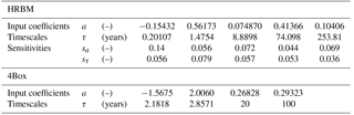
The piecewise constant approximation is adequate for time steps up to 1 year, and the piecewise linear approximation is adequate for up to decadal time steps. An overview of the performance of three representative settings (set at compile time) for the C4MIP A2 scenario is given in Table B1.
Table B1Performance and accuracy for time steps of 1–10 years relative to a reference with a time step of 0.1 year. The reference simulation is solved explicitly; otherwise an implicit solution was used. The average execution time of the time integration loop is given as a fraction of the explicit case. For atmospheric CO2 and SAT, the root mean square difference to the explicit case divided by the value range over the simulation is given. All values are for the C4MIP A2 scenario (years 1700–2100), using the HILDA ocean component and the HRBM land component with standard temperature and carbon cycle sensitivities (coupled).
The explicit solution is only implemented for the piecewise constant approximation (Eq. B2) and the implicit solution for both the piecewise constant (Eq. B2) and the piecewise linear approximation (Eq. B3). Equations (B2) and (B3) are expressed in a common equation by substituting
In the following, the implicit solution for the piecewise constant discretization is derived. Here, the fully implicit scheme for land and ocean exchange is discussed, but for stability it is only crucial to treat ocean uptake implicitly. The parameters of Eq. (B4) for this case are
First consider the equation system for carbon, assuming temperature to be known (or neglecting temperature dependence of model coefficients). Equation (B4) is applied to land carbon exchange for the constant approximation (Eq. B5),
where is the land carbon stock obtained after one time step if NPP remained constant (“constant flux commitment”), and is the change in NPP over one time step. For ocean carbon uptake,
where is the value of mS after one time step if (“zero-flux commitment”).
To solve the implicit system, the nonlinear parametrizations need to be linearized around tn−1. Linearizing ocean surface CO2 pressure as a function of surface ocean carbon and inserting in Eq. (4) yields
where Eqs. (5) and (6) were used. Similarly, NPP as a function of atmospheric carbon is linearized,
using Eq. (6).
The system is completed with the discretized budget equation (Eq. 1).
Here, en−½ is assumed to be known (though this only applies to the “forward” solution for atmospheric CO2 from emissions; solving for emissions from CO2 is also implemented in the model code).
After calculating the “committed” values from the model state at tn−1, Eqs. (B7) through (B10) are solved:
with the auxiliary variables
and, after inserting into Eq. (B6),
The remaining variables are then calculated using Eqs. (B7) and (B10), whereby first the components are calculated as in Eq. (B4) and then summed. Finally, the nonlinear parametrizations are recalculated with the updated model state.
The order of these equations matters, as the updated variables are successively inserted into the following equations. The land part is solved first, and can be substituted by an explicit step or a separate model, while keeping the ocean step implicit.
An implicit time step is also implemented for calculating SAT from RF (again, solving RF from SAT is also implemented but not discussed here). RF(tn) can be assumed as known, as atmospheric CO2 is calculated first (i.e., no linearization necessary). Applying Eq. (B4) to temperature,
where ΔTcΔ is the committed temperature for constant heat flux to the ocean, and is the change in heat flux over one time step. Equations (8), (9), and (B16) are solved for ,
Temperature change ΔTn then follows from Eq. (B16).
The case of piecewise linear approximation (Eq. B3) differs from the piecewise constant one (Eq. B2) only in a nonzero contribution of fn−1 and a slightly different budget equation,
The first difference merely changes the calculation of committed changes, and only the second difference affects the solution of the implicit time step. In practice, however, this can be neglected without loss of accuracy, and thus Eqs. (B11)–(B15) and (B17) are also used to solve the piecewise linear system (while Eq. B18 is used to close the budget).
B3 Temperature-dependent parameters
BernSCM allows for temperature-dependent model parameters for IRF-based substitute models. This generalization of the IRF approach is possible using a box model form (Sect. 2.3). Currently, temperature-dependent coefficients and timescales are implemented for the HRBM land biosphere substitute model (Appendix A2).
BernSCM updates any temperature-dependent model parameters by approximating the current temperature ΔTn by the committed temperature ΔTcΔ as defined in Eq. (B16). Accuracy is further improved by substituting ΔTcΔ for ΔTn in evaluating Eq. (B8) with temperature-dependent parametrizations.
The authors declare that they have no conflict of interest.
This work received support from the Swiss National Science Foundation
(no. 200020_172476).
Edited by: Carlos
Sierra
Reviewed by: Holger Metzler and one anonymous referee
Archer, D., Kheshgi, H., and Maier-Reimer, E.: Dynamics of fossil fuel CO2 neutralization by marine CaCO3., Global Biogeochem. Cy., 12, 259–276, 1999. a, b
Boucher, O. and Reddy, M.: Climate trade-off between black carbon and carbon dioxide emissions, Energ. Policy, 36, 193–200, 2008. a
Bruckner, T., Hooss, G., Füssel, H.-M., and Hasselmann, K.: Climate System Modeling in the Framework of the Tolerable Windows Approach: The ICLIPS Climate Model, Climatic Change, 56, 119–137, 2003. a
Budyko, M.: The effect of solar radiation variations on the climate of the earth, Tellus, 21, 611–619, https://doi.org/10.1111/j.2153-3490.1969.tb00466.x/abstract, 1969. a
Deser, C., Knutti, R., Solomon, S., and Phillips, A. S.: Communication of the role of natural variability in future North American climate, Nat. Clim. Change, 2, 775–779, 2012. a
Dickson, A. G., Sabine, C. L., and Christian, J. R.: Handbook of methods for the analysis of the various parameters of the carbon dioxide system in sea water, USDOE, 2007. a, b
Eby, M., Weaver, A. J., Alexander, K., Zickfeld, K., Abe-Ouchi, A., Cimatoribus, A. A., Crespin, E., Drijfhout, S. S., Edwards, N. R., Eliseev, A. V., Feulner, G., Fichefet, T., Forest, C. E., Goosse, H., Holden, P. B., Joos, F., Kawamiya, M., Kicklighter, D., Kienert, H., Matsumoto, K., Mokhov, I. I., Monier, E., Olsen, S. M., Pedersen, J. O. P., Perrette, M., Philippon-Berthier, G., Ridgwell, A., Schlosser, A., Schneider von Deimling, T., Shaffer, G., Smith, R. S., Spahni, R., Sokolov, A. P., Steinacher, M., Tachiiri, K., Tokos, K., Yoshimori, M., Zeng, N., and Zhao, F.: Historical and idealized climate model experiments: an intercomparison of Earth system models of intermediate complexity, Clim. Past, 9, 1111–1140, https://doi.org/10.5194/cp-9-1111-2013, 2013. a
Enting, I. G.: Laplace transform analysis of the carbon cycle, Environ. Modell. Softw., 22, 1488–1497, https://doi.org/10.1016/j.envsoft.2006.06.018, 2007. a, b
Enting, I. G., Wigley, T. M. L., and Heimann, M.: Future Emissions and Concentrations of Carbon Dioxide: Key Ocean/Atmosphere/Land analyses, Tech. rep., CSIRO. Division of Atmospheric Research, 1994. a, b
Etminan, M., Myhre, G., Highwood, E. J., and Shine, K. P.: Radiative forcing of carbon dioxide, methane, and nitrous oxide: A significant revision of the methane radiative forcing, Geophys. Res. Lett., 43, 12614–12623, 2016. a
Forster, P. M. D. F., Ramaswamy, V., Artaxo, P., Berntsen, T., Betts, R. A., Fahey, D. W. D., Haywood, J., Lean, J., Lowe, D. C. D., Myhre, G., Nganga, J., Prinn, R., Raga, G., Schulz, M., and Dorland, R. V.: Changes in Atmospheric Constituents and in Radiative Forcing, chap. 2, in: Climate Change 2007: The Physical Science Basis, Contribution of Working Group I to the Fourth Assessment Report of the Intergovernmental Panel on Climate Change, edited by: Solomon, S., Qin, D., Manning, M., Chen, Z., Marquis, M., Averyt, K. B., Tignor, M., and Miller, H. L., Cambridge Univ. Press, UK and New York, NY, USA, available at: http://www.ak-geomorphologie.de/data/Ipccreport_text_2.pdf, 2007. a
Friedlingstein, P., Cox, P., Betts, R.,Bopp, L., von Bloh, W., Brovkin, V., Cadule, P., Doney, S., Eby, M., Fung, I., Bala, G., John, J., Jones, C., Joos, F., Kato, T., Kawamiya, M., Knorr, W., Lindsay, K., Matthews, H. D., Raddatz, T., Rayner, P., Reick, C., Roeckner, E., Schnitzler, K.-G., Schnur, R., Strassmann, K., Weaver, A. J., Yoshikawa, C., and Zeng, N.: Climate – Carbon Cycle Feedback Analysis: Results from the C4MIP Model Intercomparison, J. Climate, 19, 3337–3353, https://doi.org/10.1175/JCLI3800.1, 2006. a, b, c, d, e
Frölicher, T. L., and Paynter, D. J.: Extending the relationship between global warming and cumulative carbon emissions to multi-millennial timescales, Environ. Res. Lett., 10, 075002 pp., 2015. a, b, c, d, e, f
Gattuso, J. P., Magnan, A., Billé, R., Cheung, W. W. L., Howes, E. L., Joos, F., Allemand, D., Bopp, L., Cooley, S. R., Eakin, C. M., Hoegh-Guldberg, O., Kelly, R. P., Pörtner, H. O., Rogers, A. D., Baxter, J. M., Laffoley, D., Osborn, D., Rankovic, A., Rochette, J., Sumaila, U. R., Treyer, S., and Turley, C.: Contrasting futures for ocean and society from different anthropogenic CO2 emissions scenarios, Science, 349, https://doi.org/10.1126/science.aac4722, 2015. a
Geoffroy, O., Saint-Martin, D., Bellon, G., Voldoire, A., Olivié, D. J. L., and Tytéca, S.: Transient Climate Response in a Two-Layer Energy-Balance Model. Part II: Representation of the Efficacy of Deep-Ocean Heat Uptake and Validation for CMIP5 AOGCMs, J. Climate, 26, 1859–1876, 2012a. a, b, c
Geoffroy, O., Saint-Martin, D., Olivié, D. J. L., Voldoire, A., Bellon, G., and Tytéca, S.: Transient Climate Response in a Two-Layer Energy-Balance Model. Part I: Analytical Solution and Parameter Calibration Using CMIP5 AOGCM Experiments, J. Climate, 26, 1841–1857, 2012b. a, b, c, d, e
Good, P., Gregory, J. M., and Lowe, J. A.: A step-response simple climate model to reconstruct and interpret AOGCM projections, Geophys. Res. Lett., 38, https://doi.org/10.1029/2010GL04520, 2011. a, b
Gregory, J. M., Jones, C. D., Cadule, P., and Friedlingstein, P.: Quantifying carbon cycle feedbacks, J. Climate, 22, 5232–5250, 2009. a
Gregory, J. M., Andrews, T., and Good, P.: The inconstancy of the transient climate response parameter under increasing CO2, Philos. Trans. A Math. Phys. Eng. Sci., 13, 373, https://doi.org/10.1098/rsta.2014.0417, 2015. a
Hansen, J., Lacis, A., Rind, D., and Russell, G.: Climate sensitivity: Analysis of feedback mechanisms, Geophys. Monog. Series, 29, available at:http://www.agu.org/books/gm/v029/GM029p0130/GM029p0130.shtml, 1984. a, b
Hansen, J., Sato, M., Ruedy, R., Nazarenko, L., Lacis, A., Schmidt, G. A., Russell, G., Aleinov, I., Bauer, M., Bauer, S., Bell, N., Cairns, B., Canuto, V., Chandler, M., Cheng, Y., Del Genio, A., Faluvegi, G., Fleming, E., Friend, A., Hall, T., Jackman, C., Kelley, M., Kiang, N., Koch, D., Lean, J., Lerner, J., Lo, K., Menon, S., Miller, R., Minnis, P., Novakov, T., Oinas, V., Perlwitz, J., Perlwitz, J., Rind, D., Romanou, A., Shindell, D., Stone, P., Sun, S., Tausnev, N., Thresher, D., Wielicki, B., Wong, T., Yao, M., and Zhang, S.: Efficacy of climate forcings, J. Geophys. Res.-Atmos., 110, D18104, https://doi.org/10.1029/2005JD005776 , 2005. a
Hansen, J., Ruedy, R., Sato, M., and Lo, K.: Global surface temperature change, Rev. Geophys., 48, RG4004, https://doi.org/10.1029/2010RG000345, 2010. a
Harvey, D., Gregory, J., Hoffert, M., Jain, A., Lal, M., Leemans, R., Raper, S., Wigley, T., and de Wolde, J.: IPCC Technical Paper II. An Introduction to Simple Climate Models Used in the IPCC Second Assessment Report, Intergovernmental Panel on Climate Change, 1997. a
Heck, V., Donges, J. F., and Lucht, W.: Collateral transgression of planetary boundaries due to climate engineering by terrestrial carbon dioxide removal, Earth Syst. Dynam., 7, 783–796, https://doi.org/10.5194/esd-7-783-2016, 2016. a
Heinze, C., Meyer, S., Goris, N., Anderson, L., Steinfeldt, R., Chang, N., Le Quéré, C., and Bakker, D. C. E.: The ocean carbon sink – impacts, vulnerabilities and challenges, Earth Syst. Dynam., 6, 327–358, https://doi.org/10.5194/esd-6-327-2015, 2015. a
Hijioka, Y., Takahashi, K., Hanasaki, N., Masutomi, Y., and Harasawa, H.: Comprehensive assessment of climate change impacts on Japan utilizing integrated assessment model, Association of International Research Initiatives for Environmental Studies (AIRIES), 127–133, 2009. a
Holden, P. B., Edwards, N. R., Oliver, K. I. C., Lenton, T. M., and Wilkinson, R. D.: A probabilistic calibration of climate sensitivity and terrestrial carbon change in GENIE-1, Clim. Dynam., 35, 785–806, 2010. a
Hooss, G., Voss, R., Hasselmann, K., Maier-Reimer, E., and Joos, F.: A nonlinear impulse response model of the coupled carbon cycle-climate system (NICCS), Clim. Dynam., 18, 189–202, 2001. a, b, c, d, e
Huntingford, C., Booth, B. B. B., Sitch, S., Gedney, N., Lowe, J. A., Liddicoat, S. K., Mercado, L. M., Best, M. J., Weedon, G. P., Fisher, R. A., Lomas, M. R., Good, P., Zelazowski, P., Everitt, A. C., Spessa, A. C., and Jones, C. D.: IMOGEN: an intermediate complexity model to evaluate terrestrial impacts of a changing climate, Geosci. Model Dev., 3, 679–687, https://doi.org/10.5194/gmd-3-679-2010, 2010. a
Jones, C., Robertson, E., Arora, V., Friedlingstein, P., Shevliakova, E., Bopp, L., Brovkin, V., Hajima, T., Kato, E., Kawamiya, M., Liddicoat, S., Lindsay, K., Reick, C. H., Roelandt, C., Segschneider, J., and Tjiputra, J.: Twenty-First-Century Compatible CO2 Emissions and Airborne Fraction Simulated by CMIP5 Earth System Models under Four Representative Concentration Pathways, J. Climate, 26, 4398–4413, 2013. a
Joos, F. and Bruno, M.: Pulse response functions are cost-efficient tools to model the link between carbon emissions, atmospheric CO2 and global warming, Phys. Chem. Earth, 21, 471–476, 1996. a, b, c
Joos, F., Bruno, M., Fink, R., and Siegenthaler, U.: An efficient and accurate representation of complex oceanic and biospheric models of anthropogenic carbon uptake, Tellus B, 48, 397–417, https://doi.org/10.1034/j.1600-0889.1996.t01-2-00006.x/abstract, 1996. a, b, c, d, e, f, g, h, i, j, k, l, m, n
Joos, F., Müller-Fürstenberger, G., and Stephan, G.: Correcting the carbon cycle representation: How important is it for the economics of climate change?, Environ. Model. Assess., 4, 133–140, https://doi.org/10.1023/A:1019004015342, 1999a. a
Joos, F., Plattner, G. K., Stocker, T. F., Marchal, O., and Schmittner, A.: Global warming and marine carbon cycle feedbacks on future atmospheric CO2, Science, 284, 464–467, 1999b. a
Joos, F., Prentice, I. C., Sitch, S., Meyer, R., Hooss, G., Plattner, G.-K. G., Gerber, S., and Hasselmann, K.: Global warming feedbacks on terrestrial carbon uptake under the Intergovernmental Panel on Climate Change (IPCC) emission scenarios, Global Biogeochem. Cy., 15, 891–908, 2001. a, b, c, d, e
Joos, F., Gerber, S., and Prentice, I.: Transient simulations of Holocene atmospheric carbon dioxide and terrestrial carbon since the Last Glacial Maximum, Global Biogeochem. Cy., 18, 1–18, https://doi.org/10.1029/2003GB002156, 2004. a
Joos, F., Roth, R., Fuglestvedt, J. S., Peters, G. P., Enting, I. G., von Bloh, W., Brovkin, V., Burke, E. J., Eby, M., Edwards, N. R., Friedrich, T., Frölicher, T. L., Halloran, P. R., Holden, P. B., Jones, C., Kleinen, T., Mackenzie, F. T., Matsumoto, K., Meinshausen, M., Plattner, G.-K., Reisinger, A., Segschneider, J., Shaffer, G., Steinacher, M., Strassmann, K., Tanaka, K., Timmermann, A., and Weaver, A. J.: Carbon dioxide and climate impulse response functions for the computation of greenhouse gas metrics: a multi-model analysis, Atmos. Chem. Phys., 13, 2793–2825, https://doi.org/10.5194/acp-13-2793-2013, 2013. a, b, c, d, e
Jungclaus, J. H., Bard, E., Baroni, M., Braconnot, P., Cao, J., Chini, L. P., Egorova, T., Evans, M., González-Rouco, J. F., Goosse, H., Hurtt, G. C., Joos, F., Kaplan, J. O., Khodri, M., Klein Goldewijk, K., Krivova, N., LeGrande, A. N., Lorenz, S. J., Luterbacher, J., Man, W., Maycock, A. C., Meinshausen, M., Moberg, A., Muscheler, R., Nehrbass-Ahles, C., Otto-Bliesner, B. I., Phipps, S. J., Pongratz, J., Rozanov, E., Schmidt, G. A., Schmidt, H., Schmutz, W., Schurer, A., Shapiro, A. I., Sigl, M., Smerdon, J. E., Solanki, S. K., Timmreck, C., Toohey, M., Usoskin, I. G., Wagner, S., Wu, C.-J., Yeo, K. L., Zanchettin, D., Zhang, Q., and Zorita, E.: The PMIP4 contribution to CMIP6 – Part 3: The last millennium, scientific objective, and experimental design for the PMIP4 past1000 simulations, Geosci. Model Dev., 10, 4005–4033, https://doi.org/10.5194/gmd-10-4005-2017, 2017. a
Key, R. M., Kozyr, A., Sabine, C. L., Lee, K., Wanninkhof, R., Bullister, J. L., Feely, R. A., Millero, F. J., Mordy, C., and Peng, T.: A global ocean carbon climatology: Results from Global Data Analysis Project (GLODAP), Global Biogeochem. Cy., 18, GB4031, https://doi.org/10.1029/2004GB002247, 2004. a
Knutti, R. and Sedlacek, J.: Robustness and uncertainties in the new CMIP5 climate model projections, Nat. Clim. Change, 3, 369–373, 2013. a
Landry, J.-S., Parrott, L., Price, D. T., Ramankutty, N., and Matthews, H. D.: Modelling long-term impacts of mountain pine beetle outbreaks on merchantable biomass, ecosystem carbon, albedo, and radiative forcing, Biogeosciences, 13, 5277–5295, https://doi.org/10.5194/bg-13-5277-2016, 2016. a
Le Quéré, C., Raupach, M. R., Canadell, J. G., Marland, G., Bopp, L., Ciais, P., Conway, T. J., Doney, S. C., Feely, R. A., Foster, P., Friedlingstein, P., Gurney, K., Houghton, R. A., House, J. I., Huntingford, C., Levy, P. E., Lomas, M. R., Majkut, J., Metzl, N., Ometto, J. P., Peters, G. P., Prentice, C. I., Randerson, J. T., Running, S. W., Sarmiento, J. L., Schuster, U., Sitch, S., Takahashi, T., Viovy, N., van der Werf, G. R., and Woodward, F. I.: Trends in the sources and sinks of carbon dioxide, Nat. Geosci., 2, 831–836, https://doi.org/10.1038/ngeo689, 2009. a
Le Quéré, C., Andrew, R. M., Canadell, J. G., Sitch, S., Korsbakken, J. I., Peters, G. P., Manning, A. C., Boden, T. A., Tans, P. P., Houghton, R. A., Keeling, R. F., Alin, S., Andrews, O. D., Anthoni, P., Barbero, L., Bopp, L., Chevallier, F., Chini, L. P., Ciais, P., Currie, K., Delire, C., Doney, S. C., Friedlingstein, P., Gkritzalis, T., Harris, I., Hauck, J., Haverd, V., Hoppema, M., Klein Goldewijk, K., Jain, A. K., Kato, E., Körtzinger, A., Landschützer, P., Lefèvre, N., Lenton, A., Lienert, S., Lombardozzi, D., Melton, J. R., Metzl, N., Millero, F., Monteiro, P. M. S., Munro, D. R., Nabel, J. E. M. S., Nakaoka, S.-I., O'Brien, K., Olsen, A., Omar, A. M., Ono, T., Pierrot, D., Poulter, B., Rödenbeck, C., Salisbury, J., Schuster, U., Schwinger, J., Séférian, R., Skjelvan, I., Stocker, B. D., Sutton, A. J., Takahashi, T., Tian, H., Tilbrook, B., van der Laan-Luijkx, I. T., van der Werf, G. R., Viovy, N., Walker, A. P., Wiltshire, A. J., and Zaehle, S.: Global Carbon Budget 2016, Earth Syst. Sci. Data, 8, 605–649, https://doi.org/10.5194/essd-8-605-2016, 2016. a
Levasseur, A., Cavalett, O., Fuglestvedt, J. S., Gasser, T., Johansson, D. J. A., Jørgensen, S. V., Raugei, M., Reisinger, A., Schivley, G., Strømman, A., Tanaka, K., and Cherubini, F.: Enhancing life cycle impact assessment from climate science: Review of recent findings and recommendations for application to LCA, Ecol. Indic., 71, 163–174, 2016. a
Li, S., Jarvis, A. J., and Leedal, D. T.: Are response function representations of the global carbon cycle ever interpretable?, Tellus B, 61, 361–371, 2009. a
Lord, N. S., Ridgwell, A., Thorne, M. C., and Lunt, D. J.: An impulse response function for the long tail of excess atmospheric CO2 in an Earth system model, Global Biogeochem. Cy., 30, 2–17, 2016. a
Maier-Reimer, E. and Hasselmann, K.: Transport and storage of CO2 in the ocean – an inorganic ocean-circulation carbon cycle model, Clim. Dynam., 2, 63–90, 1987. a
Mathijssen, P. J. H., Kähkölä, N., Tuovinen, J.-P., Lohila, A., Minkkinen, K., Laurila, T., and Väliranta, M.: Lateral expansion and carbon exchange of a boreal peatland in Finland resulting in 7000 years of positive radiative forcing, J. Geophys. Res.-Biogeo., 122, 562–577, https://doi.org/10.1002/2016jg003749, 2017. a
Meehl, G. A., Stocker, T. F., Collins, W. D., Friedlingstein, P., Gaye, A. T., Gregory, J. M., Kitoh, A., Knutti, R., Murphy, J. M., Noda, A., Raper, S. C. B., Watterson, I. G., Weaver, A. J., and Zhao, Z.-C.: Chapter 10: Global Climate Projections, in: Climate Change 2007: The Physical Science Basis. Contribution of Working Group I to the Fourth Assessment Report of the Intergovernmental Panel on Climate Change, edited by: Solomon, S., Qin, D., Manning, M., Chen, Z., Marquis, M., Averyt, K. B., Tignor, M., and Miller, H. L., Cambridge Univ. Press, UK and New York, NY, USA, 2007. a
Meinshausen, M., Raper, S. C. B., and Wigley, T. M. L.: Emulating coupled atmosphere-ocean and carbon cycle models with a simpler model, MAGICC6 – Part 1: Model description and calibration, Atmos. Chem. Phys., 11, 1417–1456, https://doi.org/10.5194/acp-11-1417-2011, 2011. a
Meyer, R., Joos, F., Esser, G., Heimann, M., Hooss, G., Kohlmaier, G., Sauf, W., Voss, R., and Wittenberg, U.: The substitution of high-resolution terrestrial biosphere models and carbon sequestration in response to changing CO2 and climate, Global Biogeochem. Cy., 13, 785–802, 1999. a, b, c, d, e, f, g, h, i, j
Millero, F.: Thermodynamics of the carbon dioxide system in the oceans, Geochim. Cosmochim. Ac., 59, 661–677, 1995. a
Myhre, G., Highwood, E. J., Shine, K. P., and Stordal, F.: New estimates of radiative forcing due to well mixed greenhouse gases, Geophys. Res. Lett., 25, 2715–2718, 1998. a
Myhre, G., Shindell, D., Bréon, F.-M., Collins, W., Fuglestvedt, J., Huang, J., Koch, D., Lamarque, J.-F., Lee, D., Mendoza, B., Nakajima, T., Robock, A., Stephens, G., T., T., and Zhang, H.: Anthropogenic and Natural Radiative Forcing, Cambridge University Press, Cambridge, UK and New York, NY, USA, 2013. a
Oeschger, H., Siegenthaler, U., Schotterer, U., and Gugelmann, a.: A box diffusion model to study the carbon dioxide exchange in nature, Tellus, 27, 168–192, https://doi.org/10.1111/j.2153-3490.1975.tb01671.x, 1975. a, b, c
Olsen, A., Key, R. M., van Heuven, S., Lauvset, S. K., Velo, A., Lin, X., Schirnick, C., Kozyr, A., Tanhua, T., Hoppema, M., Jutterström, S., Steinfeldt, R., Jeansson, E., Ishii, M., Pérez, F. F., and Suzuki, T.: The Global Ocean Data Analysis Project version 2 (GLODAPv2) an internally consistent data product for the world ocean, Earth Syst. Sci. Data, 8, 297–323, https://doi.org/10.5194/essd-8-297-2016, 2016. a, b
Orr, J. C. and Epitalon, J.-M.: Improved routines to model the ocean carbonate system: mocsy 2.0, Geosci. Model Dev., 8, 485–499, https://doi.org/10.5194/gmd-8-485-2015, 2015. a
Orr, J. C., Epitalon, J.-M., and Gattuso, J.-P.: Comparison of ten packages that compute ocean carbonate chemistry, Biogeosciences, 12, 1483–1510, https://doi.org/10.5194/bg-12-1483-2015, 2015. a
Pfister, P. L. and Stocker, T. F.: State-Dependence of the Climate Sensitivity in Earth System Models of Intermediate Complexity, Geophys. Res. Lett., 44, 10643–10653, 2017. a
Plattner, G.-K., Knutti, R., and Joos, F.: Long-term climate commitments projected with climate-carbon cycle models, J. Climate, 21, 2721–2751, https://doi.org/10.1175/2007JCLI1905.1, 2008. a
Prather, M., Ehhalt, D., Dentener, F., Derwent, R., Dlugokencky, E., Holland, E., Isaksen, I., Katima, J., Kirchhoff, V., Matson, P., Midgley, P., and Wang, M.: Atmospheric chemistry and greenhouse gases, in: Climate Change 2001: The Scientific Basis. Contribution of Working Group I to the Third Assessment Report of the {Intergovernmental Panel on Climate Change}, edited by: Houghton, J. T., Ding, Y., Griggs, D. J., Noguer, M., van der Linden, P. J., Dai, X., Maskell, K., and Johnson, C. A., 239–287, Cambridge University Press, Cambridge, UK and New York, NY, USA, 2001. a
Prentice, I., Farquhar, G., Fasham, M., Goulden, M., Heimann, M., Jaramillo, V., Kheshgi, H., LeQuéré, C., Scholes, R., and Wallace, D.: The carbon cycle and atmospheric CO2, 183–237, Cambridge University Press, Cambridge, UK and New York, NY, USA, 2001. a
R Core Team: R: A Language and Environment for Statistical Computing, R Foundation for Statistical Computing, Vienna, Austria, available at: https://www.R-project.org/, 2015. a
Raper, S. C. B., Gregory, J. M., and Osborn, T. J.: Use of an upwelling-diffusion energy balance climate model to simulate and diagnose A/OGCM results, Clim. Dynam., 17, 601–613, 2001. a
Raupach, M. R.: The exponential eigenmodes of the carbon-climate system, and their implications for ratios of responses to forcings, Earth Syst. Dynam., 4, 31–49, https://doi.org/10.5194/esd-4-31-2013, 2013. a, b
Revelle, R. and Suess, H.: Carbon dioxide exchange between atmosphere and ocean and the question of an increase of atmospheric CO2 during the past decades, Tellus, 9, 18–27, 1957. a
Sarmiento, J., Orr, J., and Siegenthaler, U.: A perturbation simulation of CO2 uptake in an ocean general circulation model, J. Geophys. Res., 97, 3621–3645, https://doi.org/10.1029/91JC02849, 1992. a, b, c
Schimel, D., Alves, D., Enting, I. G., Heimann, M., Joos, F., Raynaud, D., and Wigley, T. M. L.: CO2 and the carbon cycle, in: IPCC Second Scientific Assessment of Climate Change, edited by: Houghton, J. T., 76–86, Cambridge Univ. Press, New York, 1996. a
Schultz, P. A. and Kasting, J. F.: Optimal reductions in CO2 emissions., Energ. Policy, 25, 491–500, http://www.ncbi.nlm.nih.gov/pubmed/11542949, 1997. a
Sellers, W.: A global climatic model based on the energy balance of the earth-atmosphere system, J. Appl. Meteorol., 8, 392–400, 1969. a
Shine, K. P., Allan, R. P., Collins, W. J., and Fuglestvedt, J. S.: Metrics for linking emissions of gases and aerosols to global precipitation changes, Earth Syst. Dynam., 6, 525–540, https://doi.org/10.5194/esd-6-525-2015, 2015. a, b
Siegenthaler, U. and Joos, F.: Use of a simple model for studying oceanic tracer distributions and the global carbon cycle, Tellus B, 44B, 186–207, https://doi.org/10.1034/j.1600-0889.1992.t01-2-00003.x/abstract, 1992. a, b, c
Siegenthaler, U. and Oeschger, H.: Transient temperature changes due to increasing CO2 using simple models, Ann. Glaciol., 5, 153–159, 1984. a, b, c, d
Smith, C. J., Forster, P. M., Allen, M., Leach, N., Millar, R. J., Passerello, G. A., and Regayre, L. A.: FAIR v1.1: A simple emissions-based impulse response and carbon cycle model, Geosci. Model Dev. Discuss., https://doi.org/10.5194/gmd-2017-266, in review, 2017. a, b
Steinacher, M. and Joos, F.: Transient Earth system responses to cumulative carbon dioxide emissions: linearities, uncertainties, and probabilities in an observation-constrained model ensemble, Biogeosciences, 13, 1071–1103, https://doi.org/10.5194/bg-13-1071-2016, 2016. a
Steinacher, M., Joos, F., and Stocker, T. F.: Allowable carbon emissions lowered by multiple climate targets, Nature, 499, 197–201, 2013. a
Stocker, B. D., Roth, R., Joos, F., Spahni, R., Steinacher, M., Zaehle, S., Bouwman, L., Xu, R., and Prentice, I. C.: Multiple greenhouse-gas feedbacks from the land biosphere under future climate change scenarios, Nat. Clim. Change, 3, 666–672, 2013a. a
Stocker, T., Wright, D., and Mysak, L. A.: A zonally averaged, coupled ocean-atmosphere model for paleoclimate studies, J. Climate, 5, 773–797, 1992. a
Stocker, T. F., Dahe, Q., Plattner, G.-K., Alexander, L., Allen, S., Bindoff, N. L., Breon, F.-M., Church, J., Cubasch, U., Emori, S., Forster, P., Friedlingstein, P., Gillett, N., Gregory, J. M., Hartmann, D. L., Jansen, E., Kirtman, B., Knutti, R., Krishna Kumar, K., Lemke, P., Marotzke, J., Masson-Delmotte, V., Meehl, G., Mokhov, I., Piao, S., Ramaswamy, V., Randall, D., Rhein, M., Rojas, M., Sabine, C., Shindell, D., Talley, L., Vaughan, D., and Xie, S.-P.: Technical Summary, 33–115, Cambridge University Press, Cambridge, UK and New York, NY, USA, 2013. a, b
Strassmann, K. M., Joos, F., and Fischer, G.: Simulating effects of land use changes on carbon fluxes: past contributions to atmospheric CO2 increases and future commitments due to losses of terrestrial sink capacity, Tellus B, 60, 583–603, https://doi.org/10.1111/j.1600-0889.2008.00340.x, 2008. a
Takahashi, T., Olafsson, J., and Goddard, J.: Seasonal variation of CO2 and nutrients in the high-latitude surface oceans: a comparative study, Global Biogeochem. Cy., 7, 843–878, http://www.agu.org/pubs/crossref/1993/93GB02263.shtml, 1993. a, b
Tanaka, K., Kriegler, E., Bruckner, T., Hooss, G., Knorr, W., and Raddatz, T.: Aggregated Carbon Cycle, Atmospheric Chemistry, and Climate Model (ACC2) – description of the forward and inverse modes, Tech. rep., Max Planck Institute for Meteorology, 2007. a
Thompson, M. V. and Randerson, J. T.: Impulse response functions of terrestrial carbon cycle models: method and application, Glob. Change Biol., 5, 371–394, 1999. a
Urban, N. M. and Keller, K.: Probabilistic hindcasts and projections of the coupled climate, carbon cycle and Atlantic meridional overturning circulation system: a Bayesian fusion of century-scale observations with a simple model, Tellus A, 62, 737–750, 2010. a
Van Vuuren, D. P., Meinshausen, M., Plattner, G.-K., Joos, F., Strassmann, K. M., Smith, S. J., Wigley, T. M. L., Raper, S. C. B., Riahi, K., de la Chesnaye, F., den Elzen, M. G. J., Fujino, J., Jiang, K., Nakicenovic, N., Paltsev, S., Reilly, J. M., Vuuren, D. P. V., and Elzen, M. G. J. D.: Temperature increase of 21st century mitigation scenarios, P. Natl. Acad. Sci. USA, 105, 15258–15262, https://doi.org/10.1073/pnas.0711129105, 2008. van Vuuren, D. P., Lowe, J., Stehfest, E. et al. Climatic Change (2011) 104: 255. https://doi.org/10.1007/s10584-009-9764-2 a
van Vuuren, D. P. V., Lowe, J., Stehfest, E., Gohar, L., Hof, A. F., Hope, C., Warren, R., Meinshausen, M., and Plattner, G.-k.: How well do integrated assessment models simulate climate change?, Clim. Change, 104, 255, https://doi.org/10.1007/s10584-009-9764-2, 2011. a
Wigley, T. M. L. and Raper, S. C. B.: Implications for climate and sea level of revised IPCC emissions scenarios, Nature, 357, 293–300, 1992. a
Winton, M., Takahashi, K., and Held, I. M.: Importance of Ocean Heat Uptake Efficacy to Transient Climate Change, J. Climate, 23, 2333–2344, 2010. a, b
Zeebe, R. and Wolf-Gladrow, D.: CO2 in Seawater: Equilibrium, Kinetics, Isotopes, Elsevier, 2001. a