the Creative Commons Attribution 4.0 License.
the Creative Commons Attribution 4.0 License.
 | 04 Jun 2018
Cluster-based analysis of multi-model climate ensembles
Amber A. Leeson
Clustering – the automated grouping of similar data – can provide powerful and unique insight into large and complex data sets, in a fast and computationally efficient manner. While clustering has been used in a variety of fields (from medical image processing to economics), its application within atmospheric science has been fairly limited to date, and the potential benefits of the application of advanced clustering techniques to climate data (both model output and observations) has yet to be fully realised. In this paper, we explore the specific application of clustering to a multi-model climate ensemble. We hypothesise that clustering techniques can provide (a) a flexible, data-driven method of testing model–observation agreement and (b) a mechanism with which to identify model development priorities. We focus our analysis on chemistry–climate model (CCM) output of tropospheric ozone – an important greenhouse gas – from the recent Atmospheric Chemistry and Climate Model Intercomparison Project (ACCMIP). Tropospheric column ozone from the ACCMIP ensemble was clustered using the Data Density based Clustering (DDC) algorithm. We find that a multi-model mean (MMM) calculated using members of the most-populous cluster identified at each location offers a reduction of up to ∼ 20 % in the global absolute mean bias between the MMM and an observed satellite-based tropospheric ozone climatology, with respect to a simple, all-model MMM. On a spatial basis, the bias is reduced at ∼ 62 % of all locations, with the largest bias reductions occurring in the Northern Hemisphere – where ozone concentrations are relatively large. However, the bias is unchanged at 9 % of all locations and increases at 29 %, particularly in the Southern Hemisphere. The latter demonstrates that although cluster-based subsampling acts to remove outlier model data, such data may in fact be closer to observed values in some locations. We further demonstrate that clustering can provide a viable and useful framework in which to assess and visualise model spread, offering insight into geographical areas of agreement among models and a measure of diversity across an ensemble. Finally, we discuss caveats of the clustering techniques and note that while we have focused on tropospheric ozone, the principles underlying the cluster-based MMMs are applicable to other prognostic variables from climate models.


Clustering is a flexible and unsupervised numerical technique that involves the segregation of data into statistically similar groups (or “clusters”). These groups can be either determined entirely by the properties of the data themselves or guided by user constraints. Numerous clustering algorithms have been developed, each with varying degrees of complexity. The k-means clustering algorithm, for example, is a relatively simple and popular technique used in several atmospheric science problems (e.g. Mace et al., 2011; Qin et al., 2012; Austin et al., 2013; Arroyo et al., 2017). Specifically related to climate science, clustering has also been used for automated classification of various remote-sensing data (e.g. Viovy, 2000), for the interpretation of ocean-climate indices and climate patterns (Zscheischler et al., 2012; Yuan and Wood, 2012; Bador et al., 2015), in describing spatiotemporal patterns of rainfall (Muñoz Díaz and Rodrigo, 2004), and to classify surface ozone measurements from a large network of sites (Lyapina et al., 2016), among several other applications. An area for which the applicability of clustering has yet to be fully explored is in the analysis of model ensembles; a collection of comparable outputs from either multiple models or multiple realisations of the same model with perturbed physics or variations in forcing data. One example of a model ensemble is that generated during multi-model inter-comparison projects, involving chemical transport models (CTMs), climate models, or chemistry–climate models (CCMs). Such initiatives are now common and form an integral part of scientific assessment of atmospheric composition, particularly in international-policy-facing research concerning climate change. For example, recent model inter-comparison studies have considered stratospheric ozone layer recovery (Eyring et al., 2010), the climate impacts of long-term tropospheric ozone trends (Young et al., 2013; Stevenson et al., 2013), and palaeoclimatology (Braconnot et al., 2012), among others.
Multi-model ensembles are used to identify the most likely value for a given variable at a particular place and time, and a range of possible values for that variable, under the assumption that all model predictions are equally valid. In most instances, a multi-model mean (MMM) is computed from a simple arithmetic mean of all models (i.e. a one model, one vote approach), such as during the recent Atmospheric Chemistry and Climate Model Intercomparison Project (ACCMIP) studies of tropospheric ozone and the hydroxyl radical, OH (Young et al., 2013; Voulgarakis et al., 2013). For chemical species such as these, that exhibit large space–time inhomogeneity in their tropospheric abundance, a single model will rarely be universally best performing (i.e. at all locations and times). In this regard, a MMM is a useful quantity and is often considered a best estimate that includes robust features (that are still apparent after averaging) from the ensemble of models. In these circumstances however, it is also of interest to consider how estimates differ among models (model spread), which is often characterised by the standard deviation of values from all models, for example in the studies referenced above. Model spread may be used to identify areas where the best-estimate values may be more, or less, uncertain. For example, if all models agree at a given place and time then we can have confidence in the all-model MMM at that location. If all models do not agree, then more involved MMM approaches may be taken. For example, this might somehow weight individual model contributions (e.g. DelSole et al., 2013; Haughton et al., 2015; Wanders and Wood, 2016), such as based on their performance against a set of observations, thus potentially diluting spurious features from individual models. However, such approaches have been somewhat rarely implemented in recent CCM inter-comparisons and can only really be used for assessing past states, for which observations are available. Furthermore, it is not uncommon for individual models to be excluded entirely from a MMM if deemed particularly poor on the basis of an evaluation against a set of observations (e.g. Hossaini et al., 2016), or if deemed a clear or substantial outlier with respect to the majority of other models (e.g. Eyring et al., 2010).
In this study, we hypothesise that clustering techniques can provide (a) a flexible, data-driven method of testing model–observation agreement and (b) a mechanism with which to identify model development priorities. In terms of the former, clustering provides a data-driven method of grouping the model output at each place and time by how well each modelled value agrees with the ensemble as a whole. This potentially enables refinement of the ensemble by objectively identifying outlier data at a given place and time on a case-by-case basis, thus potentially removing the need to perform blanket model exclusions. In terms of the latter, clustering provides potential insight into model development needs through exploring the membership of the clusters, for example why a specific model may always be excluded from the most populous cluster at a particular location. We focus our analysis on tropospheric column ozone data from 14 atmospheric models (mostly CCMs) that took part in the ACCMIP inter-comparison (Young et al., 2013). Our specific objectives are to (i) use clustering to subsample tropospheric column ozone estimates produced by the ensemble, (ii) generate a cluster-based MMM using this subsample and evaluate this against more rudimentary approaches by comparison to observations, and (iii) explore the use of clustering as a tool to identify and visualise diversity across a model ensemble and assess the potential of this method to inform model development. We demonstrate that, as a consequence of ensemble refinement through clustering, the overall bias between modelled (i.e. MMM) and observed tropospheric column ozone is reduced, while retention of data from individual models is maximised. We also show that by using clustering to characterise model spread, we can highlight regions of time or space where our process-level understanding is presumably robust (i.e. the models are in close agreement) and where more work is needed to (a) understand why models disagree and (b) improve our understanding of underlying physical processes driving these differences. Advantages of the clustering approach over more traditional weighting methods are discussed, as are limitations of the techniques and areas of future development.
The paper is structured as follows. Section 2 provides a brief overview of cluster-based classification. Section 3 describes the principles of the proposed clustering technique, exemplified using an idealised synthetic data set. Section 4 describes the specific application of the clustering techniques to multi-model output from the ACCMIP inter-comparison. Results from the ACCMIP clustering and discussion are presented in Sect. 5. Recommendations for future research are given in Sect. 6 and we make concluding remarks in Sect. 7.
Clustering is a well-established technique for the unsupervised grouping (classification) of similar data. The unsupervised nature of clustering overcomes many of the traditional short-comings of classification techniques, e.g. no a priori information is required and classes (clusters) are data driven and may adapt to underlying changes in the data relationships. Many offline clustering algorithms are available, and no single algorithm can be considered the best for all situations. Several in-depth reviews of clustering techniques have recently been published (Aggarwal and Reddy, 2014; Nisha and Kaur, 2015; Xu and Tian, 2015); therefore here we outline only briefly the features of some common techniques, in the context of this work.
Perhaps the most popular method employed within atmospheric science is the k-means clustering algorithm (MacQueen, 1967). K means generate hyper-elliptical (i.e. elliptical over more than two dimensions), unconstrained clusters offering the benefit of fast processing and a constrained number of clusters. However, the method requires the number of clusters to be specified beforehand, limiting its usefulness in data mining and often meaning that the technique results in clusters that fit the “required answer”. Other algorithms that do not require prior knowledge of the data clusters and are therefore considered to be more data driven include subtractive clustering. This generates the required number of clusters, though it is limited by a maximum cluster radius, thereby potentially dividing natural groups of data. This technique can also be prohibitively slow where large data sets are involved, as calculations are repeated for all remaining data samples after each cluster is formed. Recently, purely data-driven techniques have been developed, including grid-based algorithms and density-based algorithms. Many of these recent developments can match, or exceed, the older techniques for speed and consistency and have the added ability to be data driven with minimal user intervention. As such, these techniques have the potential to provide powerful semi-automated insight into large data sets, such as output generated from individual atmospheric models, or a large ensemble of multiple models. In this study, we use the Data Density based Clustering (DDC) algorithm (Hyde and Angelov, 2014). The underlying principle is that data classified into a DDC-generated cluster are more similar to other data within said cluster than they are to data within other clusters. The DDC algorithm has the advantage in that the scope of each cluster is well defined. For example, maximum distances can be set, in the physical world as well as in the data space, which define the spatial regions covered by clusters and the range of data values to be considered similar. DDC matches simple techniques such as k means for speed but requires no prior information on the number of clusters. It is also robust to using larger cluster radii, as the algorithm adjusts the radii to match the data contained within the cluster. A simple application of the algorithm is described in Sect. 3 below.
In this section we explain the principles behind the proposed technique for subsampling a model ensemble through clustering, using a simple synthetic data set as an example. Chemistry–climate models attempt to simulate the atmospheric distribution of numerous chemical compounds including, for example, tropospheric ozone. Model skill and performance are typically assessed by comparison to atmospheric observations made at discrete times and locations. For a given comparison, a model may exhibit a phase offset in time or space, resulting in a large model–measurement bias, suggesting an inaccurate model – perhaps due to a process-level deficiency. However, in some cases phase offsets in space, for example, could be related to a sampling or mismatch error, particularly when comparing output from coarse-resolution models to point source observational data. Such errors are commonly encountered in inverse modelling studies, for example, that aim to derive top-down emissions of a given compound based on atmospheric observations (e.g. Chen and Prinn, 2006). To account for such, a flexible technique that looks beyond a specific space and time and that can identify similar data in the surrounding data space is required. To illustrate this, we use a simple 2-D synthetic data set as shown in Fig. 1.
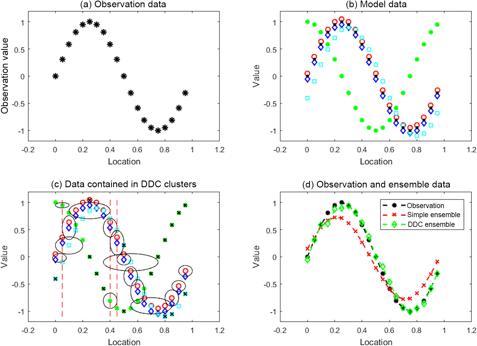
Figure 1Principles of the ensemble clustering method illustrated using a synthetic data set. (a) A synthetic spatially varying observation (X). (b) Predictions of X from four idealised models (see main text). (c) Cluster analysis of the model data sets using the DDC clustering algorithm. Ellipses represent the different clusters that are formed, and the black crosses are outliers not included in the clusters. (d) Comparison of a multi-model mean (MMM) of X derived from either a simple arithmetic mean of all model data (red) or one based on clusters (green). Observation data from panel (a) are again shown in black.
The data shown in Fig. 1 include synthetic observations (panel a) generated using a sin function. The values on the x and y axes are arbitrary and the data are intended to mimic a generic observation that is spatially non-uniform. We also consider four different sets of synthetic model data (panel b), which, with respect to the observations, exhibit (1) a small consistent positive bias (red), (2) a small consistent negative bias (dark blue), (3) a large bias (green), and (4) a slight phase offset (cyan); clearly model 3 would be considered a poor or outlier model. Taking the four models to be an ensemble, a simple MMM is generated by taking the arithmetic mean of the four model data sets at each location (i.e. no clustering involved). We also apply the DDC algorithm to the data, as shown in panel (c), to generate a cluster-based MMM. The ellipses represent the different clusters that are formed, which, as noted, can extend to nearby surrounding data space.
The DDC-based MMM is calculated by taking the mean of the data in the most populous cluster at each location (hereafter the “primary” cluster), i.e. the cluster that contains the most data samples. For example, with reference to panel (c), a cluster is formed at , . Data within this cluster are not included in the MMM at this location, as a more populous cluster at the same location (∼ 0.4, ∼ 0.6) is present. Panel (d) of Fig. 1 compares each MMM to the observed data; the model–observation bias is greatest in the case of the simple arithmetic MMM (one model, one vote approach), largely due to model 3 being included in the mean calculation. Note that each MMM is independent of the observations and in this regard the process is analogous to a multi-model prediction of a future variable (i.e. with no observational constraint).
4.1 Overview of ACCMIP datasets
The Atmospheric Chemistry and Climate Model Intercomparison Project (ACCMIP) was a multi-model initiative conducted to investigate the atmospheric abundance of key climate forcing agents, including tropospheric ozone, and their change over time (e.g. Young et al., 2013; Stevenson et al., 2013; Lamarque et al., 2013). For our purposes, we use the ACCMIP climate model data as an example of a typical multi-model ensemble on which to perform the clustering. A benefit of using ACCMIP output is that the data have been extensively handled and analysed by various groups, allowing direct comparison of our findings with published work, and the data are publicly available. We focus our analysis on modelled tropospheric column ozone data (Dobson units, DU) generated by 14 of the ACCMIP models (see Table A1). A detailed description of the models and their underlying processes can be found in the above ACCMIP publications. For each model, we analyse output from the historical simulation corresponding to the year 2000 (Young et al., 2013). Within ACCMIP, evaluation of models and the MMM was performed by comparison to a tropospheric ozone column climatology based on Ozone Monitoring Instrument (OMI) and Microwave Limb Sounder (MLS) satellite measurements (Ziemke et al., 2011). The monthly climatology extends from 60∘ N to 60∘ S; thus our cluster analysis of the ACCMIP models is applied within this latitude range (following Young et al., 2013).
Initialisation of the clustering algorithm involves selecting suitable initial cluster radii for each of the data dimensions, in this case longitude, latitude, and column ozone. In this work, we operate the clustering on a spatial basis only, to account for spatial mismatches as discussed in Sect. 3. When selecting these radii, it should be noted that the clustering algorithms perform best with data on a similar scale in each axis. To this end we scale the data to approximately 0–1 in each dimension.
4.1.1 Ozone radius selection
Modelled ozone values are scaled to approximately 0–1 using the average minimum value and average range of the data in each month as given by Eq. (1):
where O3 and O3S are the modelled and scaled ozone values, respectively, at location i as estimated by model m at time t. The initial ozone cluster radius is taken to be the average of twice the standard deviation on the model spread, Eq. (2):
where SD is the standard deviation of the ozone values of the ensemble at time t at location i, and n is the number of grid spaces. This corresponds to an initial radius of 8.3 DU (0.1523 when scaled as in Eq. 1). Note, the cluster radii evolve in a data-driven manner, excluding outliers and extreme values from the clusters. In consequence, final cluster radii using DDC range from 0.1 to 8.3 DU, with 70 % of the primary clusters with a radius < 7 DU (Fig. A1). This radius is indicative of the range of O3 data at each grid location, after outliers have been identified by the clustering process.
4.1.2 Spatial radii selection
In later sections we show that a cluster-based MMM column ozone field exhibits a lower global mean absolute bias with respect to observations, compared to a simple arithmetic MMM. This reduction in bias, due to the cluster-based subsampling, exhibits some sensitivity to the choice of initial radii in the spatial dimensions. In the latitude dimension, reduction in bias exhibits a negative correlation with radius (); i.e. bias is reduced to a lesser degree with larger radii. Results are presented from here on for initial cluster radii of 1.5 grid cells (0.0683 when normalised to 0–1) and 2.5 grid cells (0.0352) in the latitude and longitude directions, respectively, as this combination was found to give the greatest reduction in model–observation bias overall. As in Sect. 4.1.1., the cluster radii evolve in a data-driven manner and final cluster radii range from 1 to 1.6 grid cells (0.0455–0.0728) in the latitude direction, and 1–2.6 grid cells (0.0141–0.0367) in the longitude direction. Note, 92 and 99 % of primary clusters identified in this study have a radius of less than or equal to 1.1 grid cells in the latitude and longitude directions, respectively. A radius of 1.1 grid cells means that at each location, the primary cluster potentially contains data from that cell and from cells with which it shares a border. While data from nearby grid cells may affect the location of a cluster, these data are not included in cluster-based MMM calculations; the cluster-based MMM at each location is the mean of the data in the primary cluster at that location only.
4.2 Scenarios and metrics
Using the principles described above, the DDC algorithm was applied to the ACCMIP model ensemble of tropospheric column ozone on a monthly basis, and a MMM value was calculated as an average of model values in the primary cluster at each location. We also calculated MMMs of the same data using a simple arithmetic mean (all models included, equally weighted) and a sigma mean, without clustering involved in either. The sigma mean is essentially the average of all model data within 1σ of the simple arithmetic mean – i.e. a very simple outlier-removal technique. In Sect. 5.1 and 5.2, we compare each of these MMMs and evaluate their performance by comparison to the satellite-based tropospheric ozone climatology described in Sect. 4.1. In particular, we note whether or not the cluster-based MMM reduces model–observation bias with respect to the most rudimentary approach, the simple arithmetic mean, which omits no model data. In summary, three MMMs are considered: (1) simple MMM, (2) sigma MMM, and (3) cluster-based MMM. Several metrics are used in the ensuing discussion, including the model–observation mean bias (Eq. 3), and the absolute mean bias (Eq. 4), where M and O are the MMM and observed ozone field, respectively, at location i.
Table 1Observed and multi-model mean (MMM) global tropospheric ozone column (DU) between 60∘ N and 60∘ S latitude. Observations are a satellite-based climatology (Ziemke et al., 2011). Model data are from the historical (year 2000) ACCMIP simulation. The simple MMM is the arithmetic mean of all models, the sigma MMM excludes data outside of 1 standard deviation from the simple MMM, and the DDC MMM was generated through cluster-based subsampling.
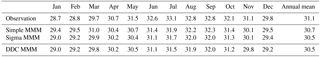
Table 2Global monthly mean bias (DU) in tropospheric ozone column (see Eq. (1)) among the various MMMs and observations presented in Table 1.
5.1 Assessment of cluster-based MMM on a global basis
We first evaluate the potential impact of clustering on MMM values by assessing the relative performance of a MMM generated using members of the primary cluster only (see Sect. 3) with respect to a simple MMM, on a global monthly mean basis. The observed column ozone data (DU) are presented in Table 1, along with equivalent MMM estimates, rows 2 and 3, obtained using a simple arithmetic mean approach – as in Table 3 of Young et al. (2013) – and a sigma mean approach. These are followed by the cluster-based MMM obtained using the DDC clustering method outlined in Sect. 3. For each MMM, the mean bias (Eq. 3) is given in Table 2. Note, the focus of this work is not to evaluate the skill of individual ACCMIP models, or the ensemble as a whole, with regard to underlying chemical processes. For that, an in-depth discussion can be obtained from Young et al. (2013). Based on Tables 1 and 2 it is clear that the ACCMIP ensemble provides a reasonably good simulation of tropospheric column ozone with respect to the observations, in a global mean sense. For example, the annual mean bias for each of the various MMMs is < 1 DU. The cluster-based MMM exhibits a bias (−0.7 DU) that is marginally greater than that obtained from the simple arithmetic MMM (−0.4 DU). However, note that the global mean biases reflect an amalgamation of positive and negative biases, masking important regional and hemispheric differences as outlined below.
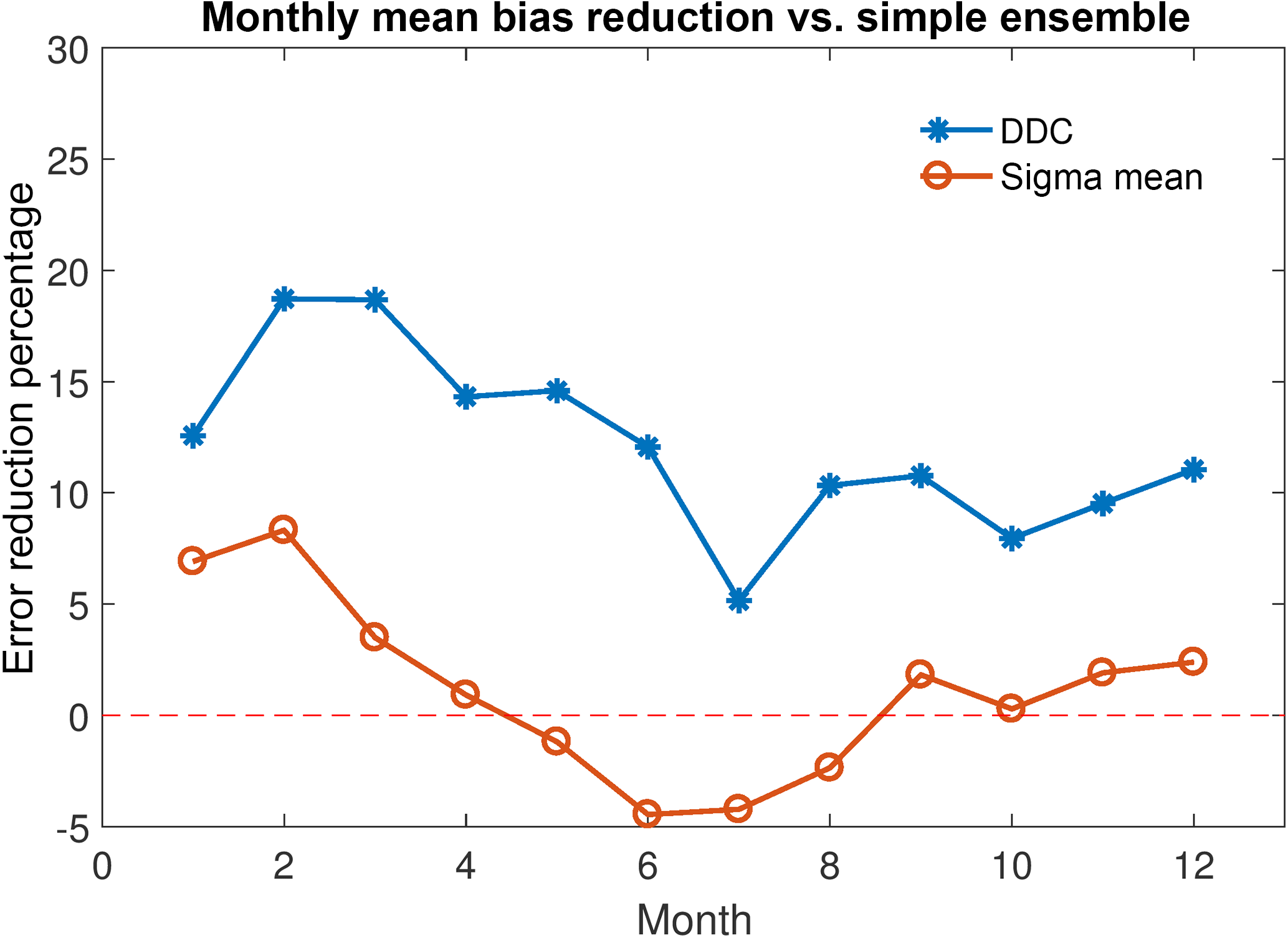
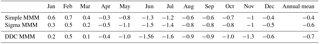
Figure 2Temporal variability in global mean (tropospheric column ozone) absolute bias reduction (%, MMM ozone − observed ozone) with respect to simple arithmetic MMM. Blue points denote bias reduction using DDC clustering to determine model inclusion into the MMM. Orange points denote bias reduction using just the model spread (1σ) to determine model inclusion into the MMM (i.e. without clustering).
Table 3As Table 2 but the absolute bias (DU) according to Eq. (2).
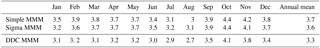
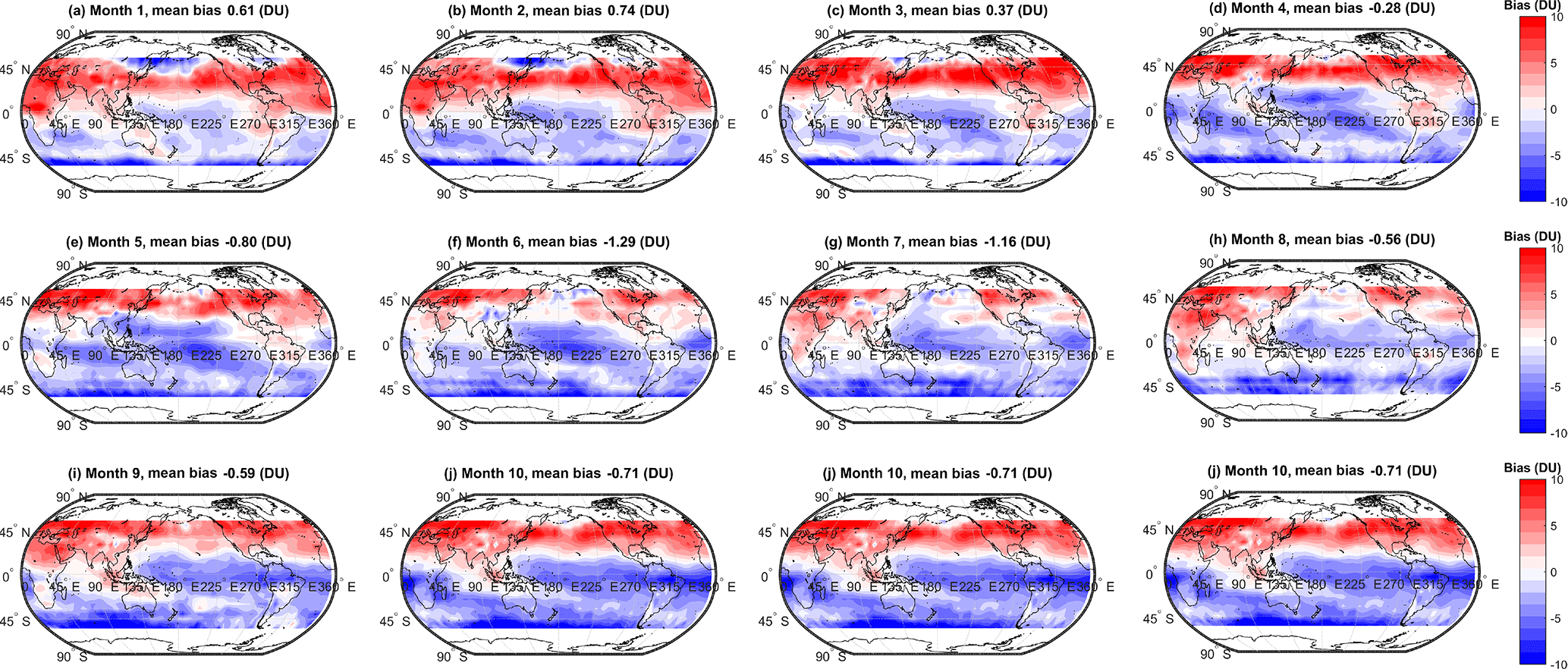
Figure 3Monthly bias (DU) between the simple arithmetic multi-model mean (MMM) tropospheric ozone column and the observed climatology. Global mean values are annotated.
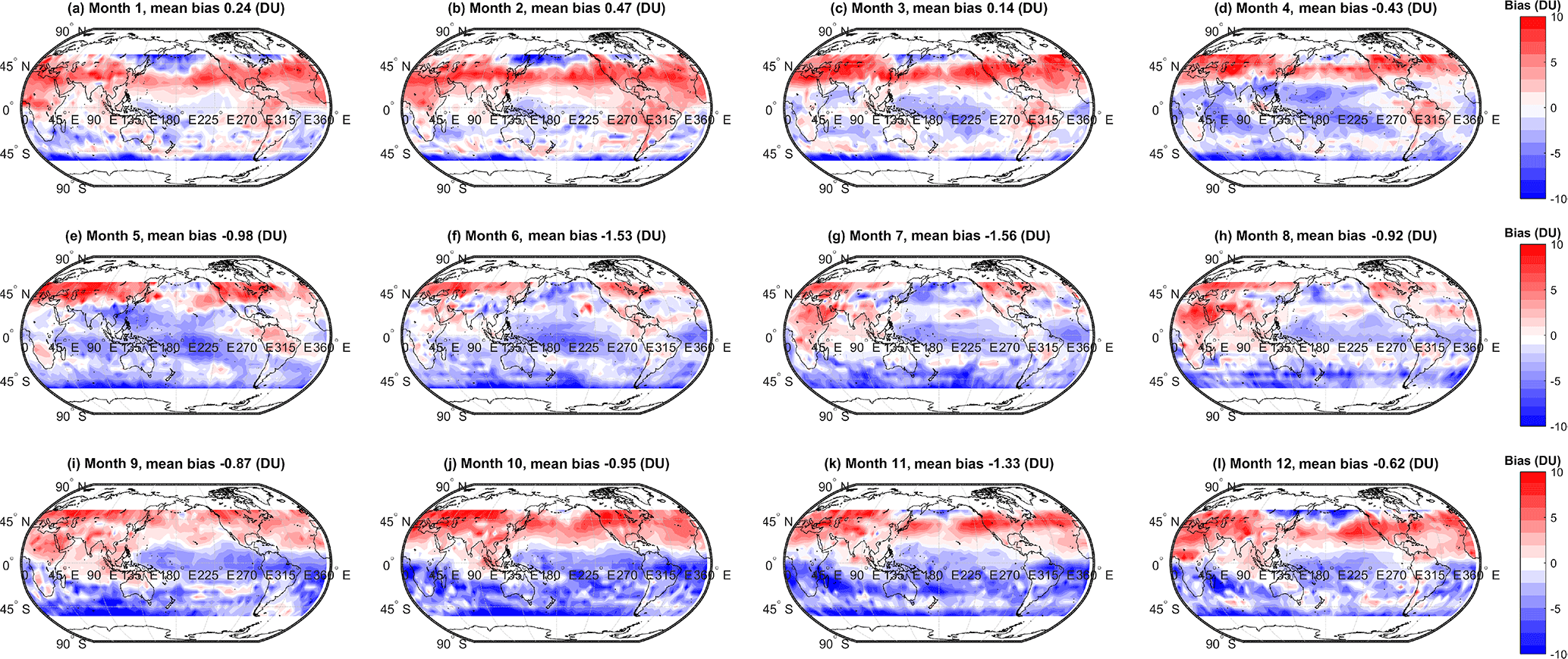

Figure 5Monthly absolute bias (DU) between the simple arithmetic multi-model mean (MMM) tropospheric ozone column and the observed climatology. Global mean values are annotated.
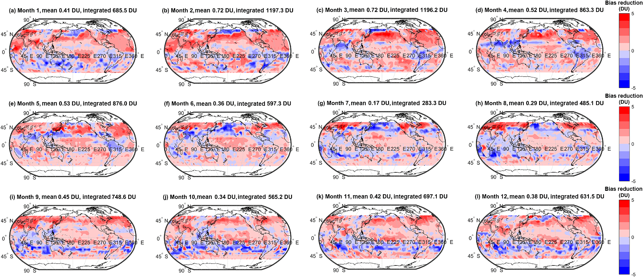
Figure 7Monthly bias reduction (DU) defined as the difference in the absolute bias between the cluster-based MMM ozone column and observations, and the simple arithmetic MMM and observations. Where the bias reduction is positive (i.e. red) the cluster-based MMM values are closer to the observations than the simple arithmetic MMM. In the title of each panel, the global mean absolute bias reduction, and the absolute bias reduction summed over all grid cells are shown.
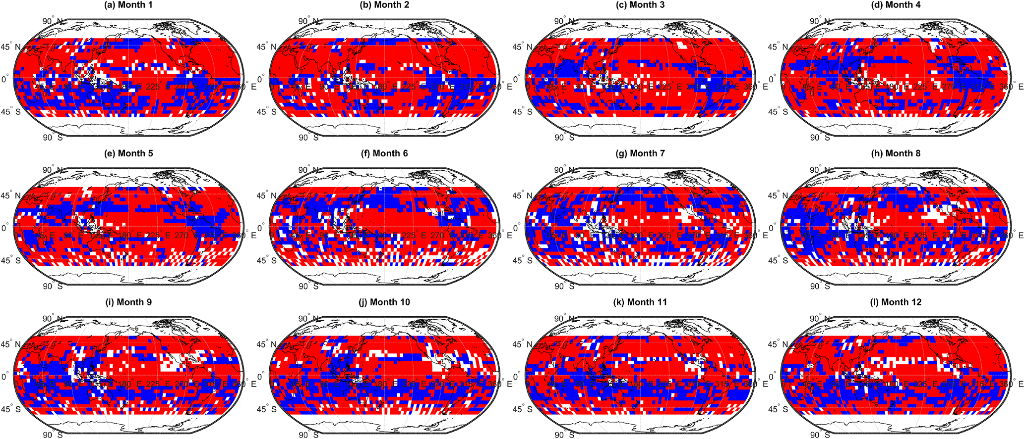
Figure 8As Fig. 7 but showing a binary of grid cells in which the model–observation bias has reduced (red), increased (blue), or not changed (white) as a result of the cluster-based ensemble subsampling.

Figure 9Histogram of the ratio of the number of members in the second most populous cluster (cluster 2) to those in the most populous cluster (cluster 1).
Table 3 is similar to Table 2 but presents the absolute biases, again on a global mean basis. The cluster-based MMM exhibits lower global mean absolute biases in all months relative to those obtained from the simple arithmetic mean approach (Fig. 2), reducing the MMM global bias by 5–19 %, depending on the month. While we do not over-interpret our findings from a model process standpoint, a distinct monthly variability is apparent in the bias reduction, with the lowest overall bias reduction in the months June–August. This is also the case for the sigma MMM, also shown in Fig. 2, which exhibits a bias increase with respect to the simple MMM during these months, despite offering a slight bias reduction overall. From Tables 1 and 2, both the observed annual mean ozone column and the absolute (model–observation) biases are highest in these months. It is perhaps unsurprising that the impact of subsampling through clustering in some months is relatively modest; if all models agree well, few (or no) model data may be excluded. In this case, the cluster-based MMM will not vary substantially from the simple arithmetic MMM and relatively little (or no) bias reduction will be observed through cluster-based subsampling. A similar situation also arises if the models have a wide spread of values at a given location; data excluded from the dominant cluster and thus not included in the cluster-based MMM may be equally divided above and below the simple MMM. In such a case, removing these data will have little effect and the cluster-based MMM will vary little from the simple MMM.
5.2 Assessment of cluster-based MMM: spatial variability
We extend the above discussion to evaluate spatial variability in the biases among the various MMMs and the observations. Spatial variability in the monthly mean bias (model − observations, DU) for the simple MMM case is shown in Fig. 3. A similar figure but for the cluster-based MMM is shown in Fig. 4. We note that our analysis agrees with Young et al. (2013); i.e. the ACCMIP ensemble tends to exhibit a high bias with respect to the observations in the Northern Hemisphere (NH) and a low bias in the Southern Hemisphere (SH, Fig. 3). The positive and negative biases largely cancel, yielding an overall small negative bias when expressed as a global mean (see Table 2). Based on Figs. 3 and 4, differences between the simple rudimentary MMM and the cluster-based MMM are difficult to fully discern by eye. The differences are more apparent when viewed as absolute biases, as given in Figs. 5 and 6. However, most striking is Fig. 7, which compares the reduction in model–observation absolute bias for the cluster-based MMM, relative to the simple arithmetic MMM. Geographically, cluster-based ensemble subsampling reduces the model–observation bias at all latitudes, though particularly in the NH and including over central Asia, Europe, and the USA – where ozone precursor emissions are generally elevated due to anthropogenic processes. Note, the ACCMIP ensemble overestimates the ozone column climatology in the NH (e.g. see Figs. 3 and 5 and previously Young et al., 2013). As such, the NH bias reduction seen in the cluster-based MMM effectively reflects some removal of data at the upper end of the model range (i.e. those models with relatively high ozone). Typical bias reduction is of the order of 1–5 DU, though larger reductions of > 5 DU are found in both hemispheres in some grid boxes.
Also apparent from Fig. 7 are regions, particularly in the SH, where the bias reduction from clustering is negative; that is, the cluster-based MMM agrees less well with the observations than the simple arithmetic MMM. To understand this, one must consider that the clustering approach relies on the density of model data points within the ensemble data space. If data from a given model are less in agreement with the other models within the ensemble, but closer to the observed value, data from said model will not be included in the cluster-based MMM. It is this feature of the clustering process that allows for the model spread of an ensemble to be readily investigated and this is discussed in following sections. In general, however, we note that the majority of the grid cells see a reduction in bias through cluster-based subsampling. For example, Fig. 8 shows a binary map plot of areas where the bias reduction is positive (i.e. red), negative (blue), and where there is no change (white). On an annual mean basis, ∼ 62 % of grid cells exhibit a positive bias reduction and a further 9 % exhibit no change in the bias. Additionally, 29 % of grid cells exhibit a negative bias reduction (i.e. biases between the cluster-based MMM and the observations are larger than those between the simple MMM and the observations). Importantly, the magnitude of the positive bias reductions greatly exceeds that of the negative changes as can be seen from the histogram given in Fig. A2. This suggests that the outliers removed from the ensemble tend to be those in relatively strong disagreement with the observations.
5.3 Insights from cluster population into model spread
Figure 9 shows a histogram of the ratio between the number of members in the second most populous cluster (cluster 2 hereafter) and the number of members in the most populous cluster (primary cluster, cluster 1 hereafter) at all points in space and time. A small number indicates that there is a significant difference, i.e. that cluster 1 has many more members than cluster 2. This suggests that the model spread is sufficiently small for most models to be included in cluster 1, and thus the models that are excluded from this cluster can be considered outliers. Conversely, if this number is large, this suggests that model spread is larger at these locations and times. As such, both cluster 1 and cluster 2 can probably be considered equivocal in terms of representing the ensemble. As can be seen from Fig. 9, in the majority of cases we consider, cluster 1 has significantly more members than cluster 2. This confirms that, in the majority of cases, subsampling the ensemble based on the membership of cluster 1 can be considered to be robust. It is important to note however that there is tail of data points with ratio values > 0.5 for which subsampling based on cluster 1 is less reasonable.
We assess the degree to which the ratio between the number of members in cluster 2 and cluster 1 varies in space and time (Fig. 10). Higher ratio values tend to occur in the mid-latitudes (suggesting greater model spread), with tropical locations exhibiting lower ratios in general. There also appears to be some seasonality to the signal; higher ratios (thus greater model spread) are more likely to occur during the summer months. It is interesting to note that regions where the ratio > 0.5 seem, by eye, to coincide with regions where the model–observation bias is increased when the ensemble is subsampled to the membership of cluster 1. This suggests that by excluding data here we are in fact removing data points which are in closer agreement with the observations. However, in general we calculate no statistically significant correlation between the ratio values and the change (if any) in bias.
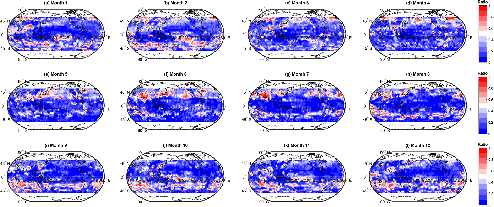
Figure 10Spatial and temporal variability in the ratio of the number of members in the second most populous cluster (cluster 2) to those in the most populous cluster (cluster 1).
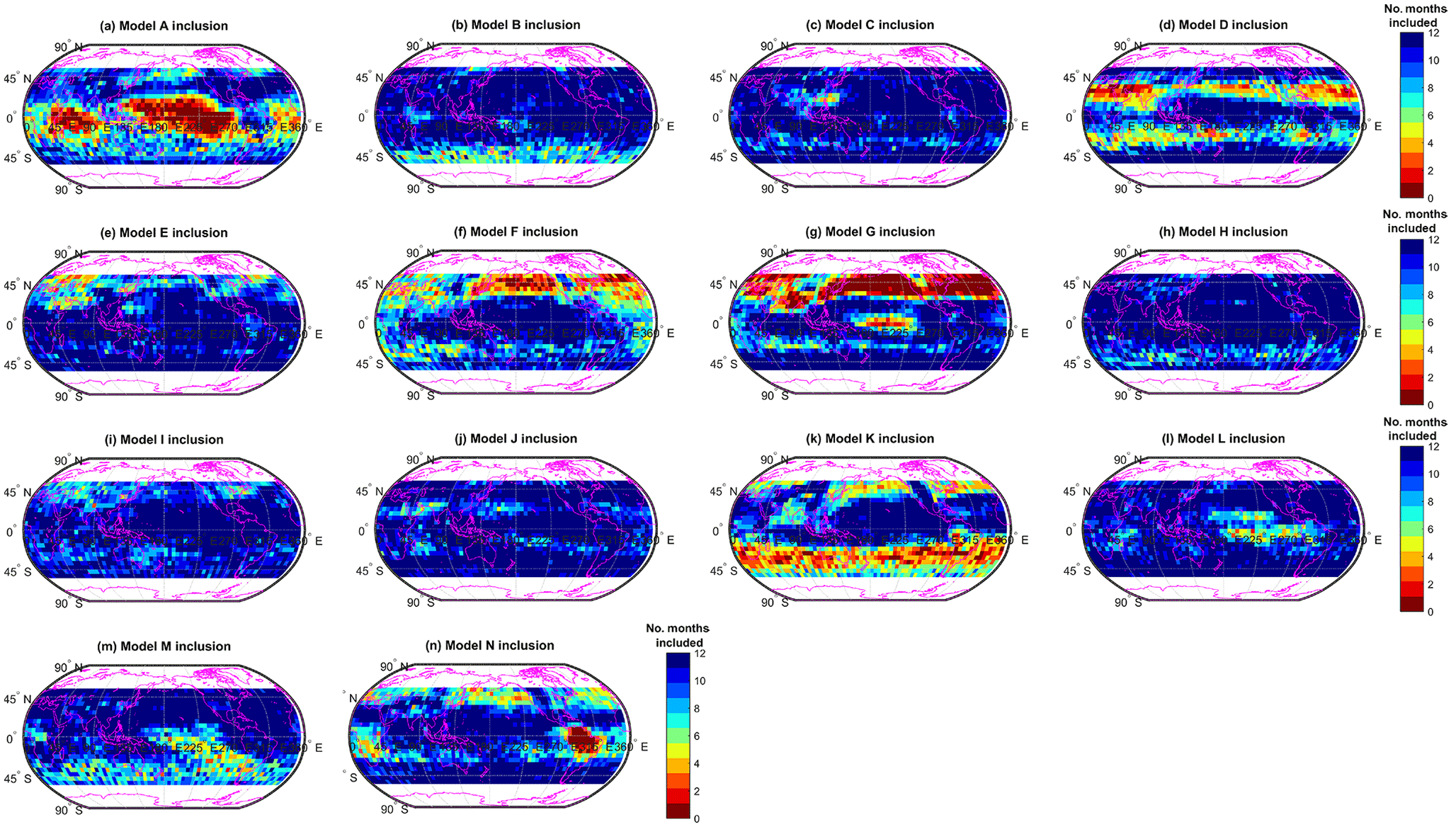
Figure 11Number of months each model (names removed, labelled A–N) is included in the primary cluster. For a given region, models that are seldom included (i.e. a low numbers of months) differ more from the ensemble pack.
5.4 Insights from cluster membership into model agreement and spread
We investigate the degree to which individual models are typically included or excluded from the primary cluster by counting the number of months when that model is included at each location, as shown in Fig. 11. This offers a simple mechanism to visualise model spread more generally; outlier models are more often excluded, and models which fall in the pack are more often included. This information can be used together with Fig. 6 as a means to identify which models are potentially driving ensemble mean model–observation biases, and so identify priorities for model development. We outline some examples here but do not intend this to be exhaustive, but rather more indicative of how this reasoning and approach potentially provides a useful framework to guide further investigation.
Model G, for example, differs significantly from the ensemble pack in the mid-latitude NH, over both land and ocean, as evidenced by the fact that it is virtually always excluded in this region. Similarly, model N is consistently different over South America in particular; this potentially points towards a spurious model feature concerning ozone – e.g. regional precursor emissions here. Model K is often not included in the primary cluster at SH locations, suggesting that it differs substantially from the other models in this region. However, this does not necessarily suggest that the model is in disagreement with observations in the SH, merely that model K differs from the others. In fact, as was noted earlier, the cluster-based MMM agrees less well with observations in the SH, compared to the simple MMM, meaning that model K – which will have been excluded during the clustering process – could be closer to reality (observations) in this region, relative to the other models. We note that all models are included at some locations, i.e. there is no blanket exclusion of certain models from the primary cluster. In fact, some models, e.g. models C, I, and J, are almost always included in the primary cluster at each location. This suggests that these models produce ozone fields that are somewhat typical and in broad agreement with the ensemble mean.
While the principles presented here are robust and proven to be beneficial, some areas of methodological development or refinement have been identified. Firstly, we intend to explore the application of clustering in time, in addition to the mainly spatial methods presented here. Further, at present clusters are allowed to form in three dimensions: latitude, longitude, and the predicted column ozone. In this way we allow for a degree of uncertainty in the model output. Future work will build on this by developing methods to incorporate estimates of standard deviation and range associated with the modelled mean values in our techniques, thus enabling a more sophisticated treatment of uncertainty. We have also identified areas of methodological development in terms of our method for calculating a cluster-based MMM. For example, we currently assign all model data from the ensemble to a cluster and then we use this information to include or exclude model data in an MMM. We have yet to consider the impact of weighting data within a cluster by (a) distance from cluster centre and (b) distance from the location of the simple MMM (as opposed to a simple include or exclude rule). Similarly, in future work we will look at the possibility of weighting ensemble members according to their cluster membership, i.e. members of the most populous cluster contributing more to the MMM than the less populous clusters and clear outliers. Finally, forthcoming model inter-comparison initiatives, e.g. CMIP6, will provide an excellent opportunity to apply our methods to consider parameters other than ozone that are of atmospheric interest (e.g. other short-lived climate forcing agents).
In this paper, we have investigated the applicability of an advanced data clustering method as an analytical–diagnostic tool with which to examine multi-model climate output. Relative to more rudimentary approaches, clustering offers a flexible method to evaluate inter-model differences. The technique operates by grouping data at a given location based on the density of data points. The flexibility arises as the clustering method examines surrounding data space (e.g. spatially) to account for small spatial and mismatch errors (e.g. arising due to differing coarse model grids), thus offering an advantage over more traditional inter-comparison methods. The clustering technique was applied to simulated fields of tropospheric column ozone from the 14 CCMs that took part in the ACCMIP model inter-comparison. We demonstrate that a cluster-based MMM tropospheric column ozone field, calculated using those data which are members of the most populous cluster at each location, exhibits a lower absolute bias with respect to observations, compared to a simple arithmetic MMM approach. On a global mean basis this reduction is observed in all months and, in some months, is as high as ∼ 20 %. However, we also note that at 28 % of places and times, the cluster-based MMM exhibits a higher absolute bias with respect to observations than a simple arithmetic MMM. We attribute this to apparent outlier model data, which are in closer agreement with observations, being excluded from the cluster-based MMM through cluster-based subsampling. Additionally, we show that clustering offers a useful framework in which to readily identify and visualise model spread and outliers. We suggest that such techniques could prove valuable in the identification of model development areas and provide insight surrounding regional strengths and deficiencies of specific models (or an ensemble as a whole), and to help characterise uncertainty. Finally, while we have focused on tropospheric ozone, we note that there is broad scope to develop the application of these techniques within the atmospheric sciences to examine other compounds relevant to climate.
The clustering code, including demo software (Hyde, 2017) and related data sets, used to generate the results in this paper is available via GitHub: https://rhyde67.github.io/CATaCoMB-Climate-Model-Ensemble/. The latest release is available via Zenodo, https://doi.org/10.5281/zenodo.1119038. The model data files are available at the Centre for Environmental Data Analysis (CEDA): http://www.ceda.ac.uk/. A summary of ACCMIP models and data sets used in this work can be found in Appendix A.
Table A1Summary and citations for the ACCMIP models and data sets used in this work.
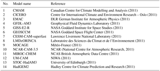
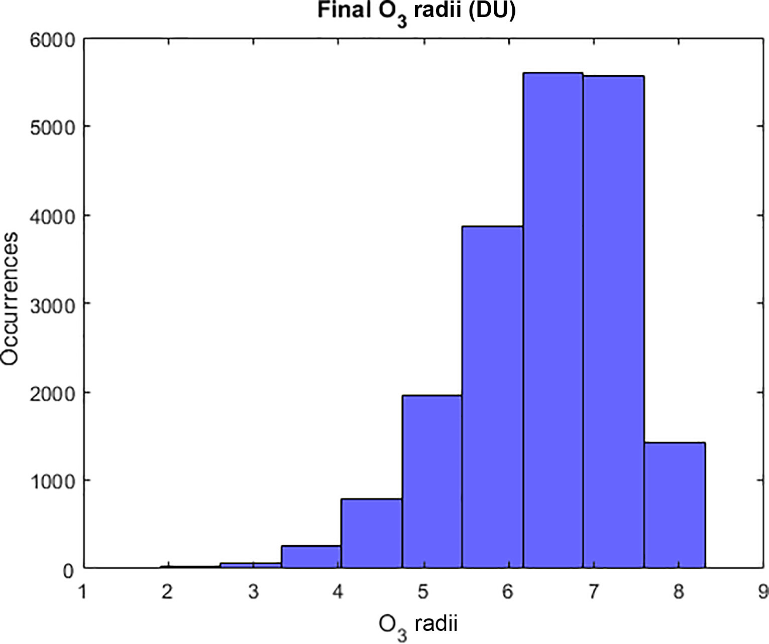
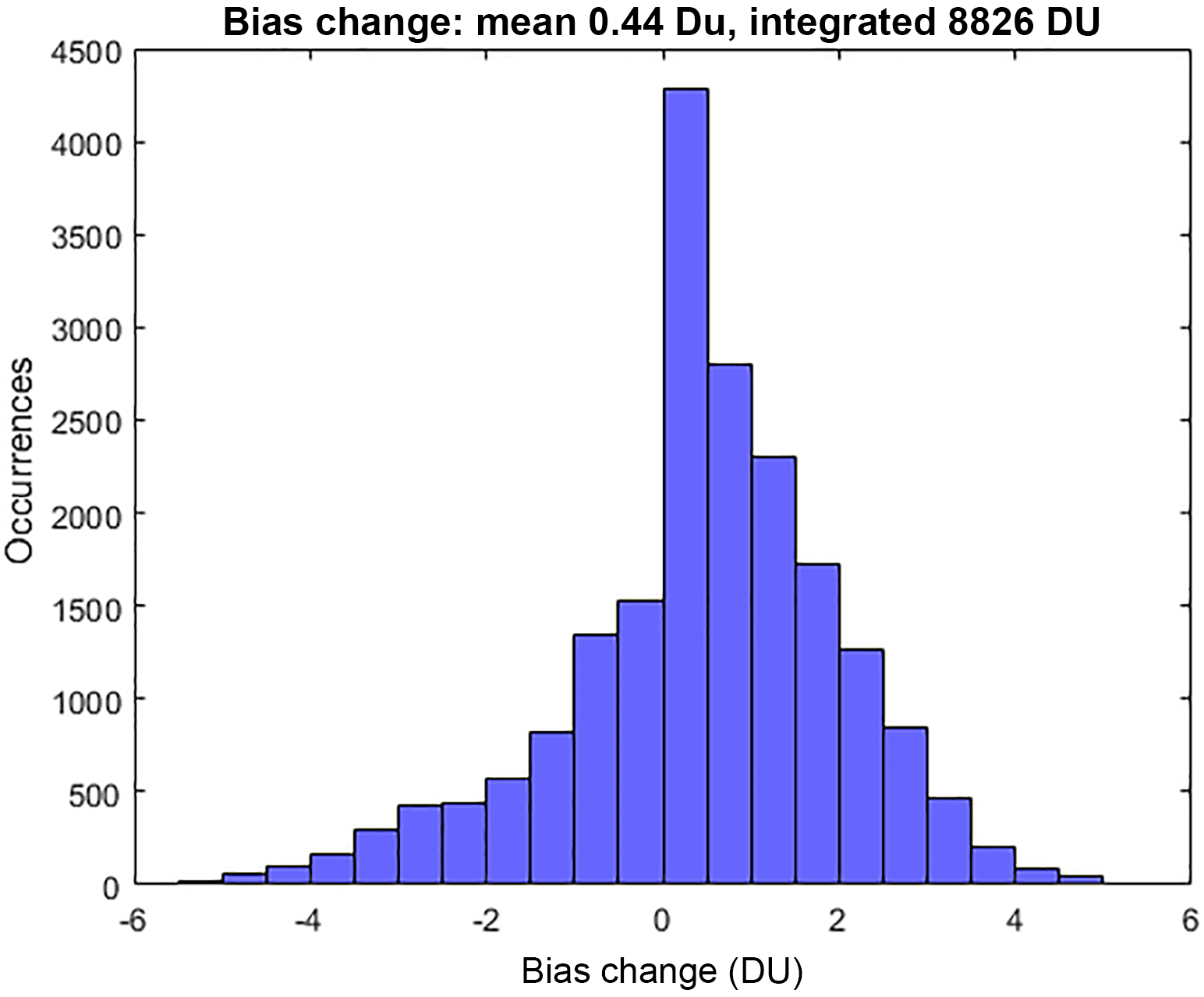
Figure A2Magnitude of the difference between annually integrated model–observation ozone biases (DU) calculated using a cluster-based MMM and a simple, all-model MMM (see Sect. 5.2).
The authors declare that they have no conflict of interest.
This work was supported by the EPSRC through a pilot study (Advanced Data
Clustering for Climate Science Applications, RFFLP027) as part of the
Research on Changes of Variability and Environmental Risk (ReCoVER) program.
R. Hossaini is also supported by an NERC Independent Research Fellowship
(NE/N014375/1). We thank Paul Young for data access and helpful discussions.
Edited by: Jeremy Fyke
Reviewed by: Martin Schultz and one anonymous referee
Aggarwal, C. C. and Reddy, C. K. (Eds.): DATA Clustering Algorithms and Applications, CRC Press, Boca Raton, available at: https://www.crcpress.com/Data-Clustering-Algorithms-and-Applications/Aggarwal-Reddy/p/book/9781466558212 (last access: 28 May 2018), 2014.
Arroyo, A., Tricio, V., Herrero, A., and Corchado, E.: Time Analysis of Air Pollution in a Spanish Region Through k-means, in: International Joint Conference SOCO'16- CISIS'16-ICEUTE'16, edited by: Grana, M., Lopez Guede, J. M., Etxaniz, O., Herrero, A., Quintian, H., and Corchado, E., Advances in Intelligent Systems and Computing, 527 63–72, https://doi.org/10.1007/978-3-319-47364-2, 2017.
Austin, E., Coull, B. A., Zanobetti, A., and Koutrakis, P.: A framework to spatially cluster air pollution monitoring sites in US based on the PM2.5 composition, Environ. Int., 59, 244–254, https://doi.org/10.1016/j.envint.2013.06.003, 2013.
Bador, M., Naveau, P., Gilleland, E., Castellà, M., and Arivelo, T.: Spatial clustering of summer temperature maxima from the CNRM-CM5 climate model ensembles and E-OBS over Europe, Weather Clim. Extrem., 9, 17–24, 2015.
Braconnot, P., Harrison, S. P., Kageyama, M., Bartlein, P. J., Masson-Delmotte, V., Abe-Ouchi, A., Otto-Bliesner, B., and Zhao, Y.: Evaluation of climate models using palaeoclimatic data, Nat. Clim. Change, 2, 417–424, https://doi.org/10.1038/NCLIMATE1456, 2012.
Canadian Centre for Climate Modelling and Analysis: ACCMIP: CCCma (Canadian Centre for Climate Modelling and Analysis) climate model output, available at: http://catalogue.ceda.ac.uk/uuid/933f1028b637a847a6f2e1729cc3237c (last access: 28 May 2018), 2011.
Centre for International Climate and Environment Research – Oslo: ACCMIP: CICERO (Centre for International Climate and Environment Research, Oslo) climate model output, available at: http://catalogue.ceda.ac.uk/uuid/798b90d6eec65e6436c34c329df8b9c4 (last access: 28 May 2018), 2011.
Chen, Y.-H. and Prinn, R. G.: Estimation of atmospheric methane emissions between 1996 and 2001 using a three-dimensional global chemical transport model, J. Geophys. Res.-Atmos., 111, D10307, https://doi.org/10.1029/2005JD006058, 2006.
DelSole, T., Yang, X., and Tippett, M. K.: Is unequal weighting significantly better than equal weighting for multi-model forecasting?, Q. J. Roy. Meteor. Soc., 139, 176–183, https://doi.org/10.1002/qj.1961, 2013.
DLR German Institute for Atmospheric Physics: ACCMIP: DLR (German Aerospace Centre) climate model output, available at: http://catalogue.ceda.ac.uk/uuid/4cbf297603e8fec86cbd81abe0591377 (last access: 28 May 2018), 2011.
Eyring, V., Cionni, I., Bodeker, G. E., Charlton-Perez, A. J., Kinnison, D. E., Scinocca, J. F., Waugh, D. W., Akiyoshi, H., Bekki, S., Chipperfield, M. P., Dameris, M., Dhomse, S., Frith, S. M., Garny, H., Gettelman, A., Kubin, A., Langematz, U., Mancini, E., Marchand, M., Nakamura, T., Oman, L. D., Pawson, S., Pitari, G., Plummer, D. A., Rozanov, E., Shepherd, T. G., Shibata, K., Tian, W., Braesicke, P., Hardiman, S. C., Lamarque, J. F., Morgenstern, O., Pyle, J. A., Smale, D., and Yamashita, Y.: Multi-model assessment of stratospheric ozone return dates and ozone recovery in CCMVal-2 models, Atmos. Chem. Phys., 10, 9451–9472, https://doi.org/10.5194/acp-10-9451-2010, 2010.
Geophysical Fluid Dynamics Laboratory: ACCMIP: GFDL (Geophysical Fluid Dynamics Laboratory) climate model output, available at: http://catalogue.ceda.ac.uk/uuid/4f766fc704885bd8abc2e8cf8da18074 (last access: 28 May 2018), 2011.
Hadley Centre for Climate Prediction and Research: ACCMIP: UKMO (UK Meteorological Office) climate model output, available at: http://catalogue.ceda.ac.uk/uuid/d425df86b1c93132f91fcb1712eb4231 (last access: 28 May 2018), 2011.
Haughton, N., Abramowitz, G., Pitman, A., and Phipps, S. J.: Weighting climate model ensembles for mean and variance estimates, Clim. Dynam., 45, 3169–3181, https://doi.org/10.1007/s00382-015-2531-3, 2015.
Hossaini, R., Patra, P. K., Leeson, A. A., Krysztofiak, G., Abraham, N. L., Andrews, S. J., Archibald, A. T., Aschmann, J., Atlas, E. L., Belikov, D. A., Bönisch, H., Carpenter, L. J., Dhomse, S., Dorf, M., Engel, A., Feng, W., Fuhlbrügge, S., Griffiths, P. T., Harris, N. R. P., Hommel, R., Keber, T., Krüger, K., Lennartz, S. T., Maksyutov, S., Mantle, H., Mills, G. P., Miller, B., Montzka, S. A., Moore, F., Navarro, M. A., Oram, D. E., Pfeilsticker, K., Pyle, J. A., Quack, B., Robinson, A. D., Saikawa, E., Saiz-Lopez, A., Sala, S., Sinnhuber, B.-M., Taguchi, S., Tegtmeier, S., Lidster, R. T., Wilson, C., and Ziska, F.: A multi-model intercomparison of halogenated very short-lived substances (TransCom-VSLS): linking oceanic emissions and tropospheric transport for a reconciled estimate of the stratospheric source gas injection of bromine, Atmos. Chem. Phys., 16, 9163–9187, https://doi.org/10.5194/acp-16-9163-2016, 2016.
Hyde, R.: RHyde67/CATaCoMB-Climate-Model-Ensemble: Initial Release (Version v0.1.1), Zenodo, https://doi.org/10.5281/ZENODO.1119039, 2017.
Hyde, R. and Angelov, P.: Data density based clustering, in: 2014 14th UK Workshop on Computational Intelligence (UKCI), 2014 14th UK Workshop on Computational Intelligence (UKCI), Bradford, UK, 8–10 September 2014, https://doi.org/10.1109/UKCI.2014.6930157, 2014.
Laboratoire des Sciences du Climat et de l'Environnement: ACCMIP: LSCE (Climate and Environment Sciences Laboratory) climate model output, available at: http://catalogue.ceda.ac.uk/uuid/76176d487a5757234d3075175675246a (last access: 28 May 2018), 2011.
Lamarque, J.-F., Shindell, D. T., Josse, B., Young, P. J., Cionni, I., Eyring, V., Bergmann, D., Cameron-Smith, P., Collins, W. J., Doherty, R., Dalsoren, S., Faluvegi, G., Folberth, G., Ghan, S. J., Horowitz, L. W., Lee, Y. H., MacKenzie, I. A., Nagashima, T., Naik, V., Plummer, D., Righi, M., Rumbold, S. T., Schulz, M., Skeie, R. B., Stevenson, D. S., Strode, S., Sudo, K., Szopa, S., Voulgarakis, A., and Zeng, G.: The Atmospheric Chemistry and Climate Model Intercomparison Project (ACCMIP): overview and description of models, simulations and climate diagnostics, Geosci. Model Dev., 6, 179–206, https://doi.org/10.5194/gmd-6-179-2013, 2013.
Lawrence Livermore National Laboratory: ACCMIP: LLNL (Lawrence Livermore National Laboratory) climate model output, available at: http://catalogue.ceda.ac.uk/uuid/81942748c9f4e15632d0082d9d84a37d (last access: 28 May 2018), 2011.
Lyapina, O., Schultz, M. G., and Hense, A.: Cluster analysis of European surface ozone observations for evaluation of MACC reanalysis data, Atmos. Chem. Phys., 16, 6863–6881, https://doi.org/10.5194/acp-16-6863-2016, 2016.
Mace, A., Sommariva, R., Fleming, Z., and Wang, W.: Adaptive K-Means for Clustering Air Mass Trajectories, in: IIntelligent Data Engineering and Automated Learning – IDEAL 2011., edited by: Yin, H., Wang, W., and Rayward Smith, V., Lecture Notes in Computer Science, vol. 6936, Springer, Berlin, Heidelberg, 2011.
MacQueen, J. B.: Some Methods for classification and analysis of multivariate observations, Procedings of the Fifth Berkeley Symposium on Math, Statistics, and Probability, 1, 281–297, 1967.
Météo-France: ACCMIP: MeteoFrance (French National Meteorological Service) climate model output, available at: http://catalogue.ceda.ac.uk/uuid/5fd4b24429ed256e0572ebf38f860343 (last access: 28 May 2018), 2011.
Muñoz-Díaz, D. and Rodrigo, F. S.: Spatio-temporal patterns of seasonal rainfall in Spain (1912–2000) using cluster and principal component analysis: comparison, Ann. Geophys., 22, 1435–1448, https://doi.org/10.5194/angeo-22-1435-2004, 2004.
NASA Goddard Institute for Space Studies: ACCMIP: GISS (Goddard Institute for Space Studies) climate model output, available at: http://catalogue.ceda.ac.uk/uuid/e6a0f9fa6e8a5cce53a2ce56c4eb0426 (last access: 28 May 2018), 2011.
NCAR (National Centre for Atmospheric Research), Lamarque, J., Shindell, D., Eyring, V., Collins, W., Nagashima, T., Szopa, S., and Zeng, G.: ACCMIP: NCAR (National Centre for Atmospheric Research) climate model output, available at: http://catalogue.ceda.ac.uk/uuid/6a1c68641c65075d2cd24eb899ec6c45 (last access: 28 May 2018), 2011.
NCAS British Atmospheric Data Centre: ACCMIP: NIES (National Institute for Environmental Studies) climate model output, available at: http://catalogue.ceda.ac.uk/uuid/d8fd67c8235a9935545da54534376ff8 (last access: 28 May 2018), 2011.
Nisha and Kaur, P. J.: A Survey of Clustering Techniques and Algorithms, 2nd International Conference on Computing for Sustainable Global Development (INDIACom), 304–307, https://doi.org/10.5120/1326-1808, 2015.
NIWA: ACCMIP: NIWA (National Institute of Water and Atmospheric Research, New Zealand) climate model output, available at: http://catalogue.ceda.ac.uk/uuid/3c5beadb79d969bcf4796b0a1db0bea6 (last access: 28 May 2018), 2011.
University of Edinburgh: ACCMIP: UEDI (University of Edinburgh) climate model output. NCAS British Atmospheric Data Centre, available at: http://catalogue.ceda.ac.uk/uuid/750818091eb772add8e9e0f7df735a7b (last access: 28 May 2018), 2011.
Qin, N., Kong, X.-Z., Zhu, Y., He, W., He, Q.-S., Yang, B., Ou-Yang, H.-L., Liu, W.-X., Wang, Q.-M., and Xu, F.-L.: Distributions, Sources, and Backward Trajectories of Atmospheric Polycyclic Aromatic Hydrocarbons at Lake Small Baiyangdian, Northern China, Sci. World J., 2012, 4163211, https://doi.org/10.1100/2012/416321, 2012.
Stevenson, D. S., Young, P. J., Naik, V., Lamarque, J.-F., Shindell, D. T., Voulgarakis, A., Skeie, R. B., Dalsoren, S. B., Myhre, G., Berntsen, T. K., Folberth, G. A., Rumbold, S. T., Collins, W. J., MacKenzie, I. A., Doherty, R. M., Zeng, G., van Noije, T. P. C., Strunk, A., Bergmann, D., Cameron-Smith, P., Plummer, D. A., Strode, S. A., Horowitz, L., Lee, Y. H., Szopa, S., Sudo, K., Nagashima, T., Josse, B., Cionni, I., Righi, M., Eyring, V., Conley, A., Bowman, K. W., Wild, O., and Archibald, A.: Tropospheric ozone changes, radiative forcing and attribution to emissions in the Atmospheric Chemistry and Climate Model Intercomparison Project (ACCMIP), Atmos. Chem. Phys., 13, 3063–3085, https://doi.org/10.5194/acp-13-3063-2013, 2013.
Viovy, N.: Automatic Classification of Time Series (ACTS): A new clustering method for remote sensing time series, Int. J. Remote Sens., 21, 1537–1560, https://doi.org/10.1080/014311600210308, 2000.
Voulgarakis, A., Naik, V., Lamarque, J.-F., Shindell, D. T., Young, P. J., Prather, M. J., Wild, O., Field, R. D., Bergmann, D., Cameron-Smith, P., Cionni, I., Collins, W. J., Dalsøren, S. B., Doherty, R. M., Eyring, V., Faluvegi, G., Folberth, G. A., Horowitz, L. W., Josse, B., MacKenzie, I. A., Nagashima, T., Plummer, D. A., Righi, M., Rumbold, S. T., Stevenson, D. S., Strode, S. A., Sudo, K., Szopa, S., and Zeng, G.: Analysis of present day and future OH and methane lifetime in the ACCMIP simulations, Atmos. Chem. Phys., 13, 2563–2587, https://doi.org/10.5194/acp-13-2563-2013, 2013.
Wanders, N. and Wood, E. F.: Improved sub-seasonal meteorological forecast skill using weighted multi-model ensemble simulations, Environ. Res. Lett., 11, 94007, https://doi.org/10.1088/1748-9326/11/9/094007, 2016.
Xu, D. and Tian, Y.: A Comprehensive Survey of Clustering Algorithms, Annals of Data Science, 2, 165–193, https://doi.org/10.1007/s40745015-0040-1, 2015.
Young, P. J., Archibald, A. T., Bowman, K. W., Lamarque, J.-F., Naik, V., Stevenson, D. S., Tilmes, S., Voulgarakis, A., Wild, O., Bergmann, D., Cameron-Smith, P., Cionni, I., Collins, W. J., Dalsøren, S. B., Doherty, R. M., Eyring, V., Faluvegi, G., Horowitz, L. W., Josse, B., Lee, Y. H., MacKenzie, I. A., Nagashima, T., Plummer, D. A., Righi, M., Rumbold, S. T., Skeie, R. B., Shindell, D. T., Strode, S. A., Sudo, K., Szopa, S., and Zeng, G.: Pre-industrial to end 21st century projections of tropospheric ozone from the Atmospheric Chemistry and Climate Model Intercomparison Project (ACCMIP), Atmos. Chem. Phys., 13, 2063–2090, https://doi.org/10.5194/acp-13-2063-2013, 2013.
Yuan, X. and Wood, E. F.: On the clustering of climate models in ensemble seasonal forecasting, Geophys. Res. Lett., 39, L18701, https://doi.org/10.1029/2012GL052735, 2012.
Ziemke, J. R., Chandra, S., Labow, G. J., Bhartia, P. K., Froidevaux, L., and Witte, J. C.: A global climatology of tropospheric and stratospheric ozone derived from Aura OMI and MLS measurements, Atmos. Chem. Phys., 11, 9237–9251, https://doi.org/10.5194/acp-11-9237-2011, 2011.
Zscheischler, J., Mahecha, M. D., and Harmeling, S.: Climate Classifications: the Value of Unsupervised Clustering, Procedia Comput. Sci., 9, 897–906, https://doi.org/10.1016/j.procs.2012.04.096, 2012.
- Abstract
- Introduction
- A brief overview of cluster-based classification
- The principles of cluster-based ensemble subsampling
- Specific application of clustering to ACCMIP model data
- Results and discussion
- Future work
- Concluding remarks
- Code and data availability
- Appendix A
- Competing interests
- Acknowledgements
- References