the Creative Commons Attribution 4.0 License.
the Creative Commons Attribution 4.0 License.
 | 08 Jun 2018
WRF and WRF-Chem v3.5.1 simulations of meteorology and black carbon concentrations in the Kathmandu Valley
Andrea Mues
Aurelia Lupascu
Maheswar Rupakheti
Friderike Kuik
Mark G. Lawrence
An evaluation of the meteorology simulated using the Weather Research and Forecast (WRF) model for the region of south Asia and Nepal with a focus on the Kathmandu Valley is presented. A particular focus of the model evaluation is placed on meteorological parameters that are highly relevant to air quality such as wind speed and direction, boundary layer height and precipitation. The same model setup is then used for simulations with WRF including chemistry and aerosols (WRF-Chem). A WRF-Chem simulation has been performed using the state-of-the-art emission database, EDGAR HTAP v2.2, which is the Emission Database for Global Atmospheric Research of the Joint Research Centre (JRC) of the European Commission, in cooperation with the Task Force on Hemispheric Transport of Air Pollution (TF HTAP) organized by the United Nations Economic Commission for Europe, along with a sensitivity simulation using observation-based black carbon emission fluxes for the Kathmandu Valley. The WRF-Chem simulations are analyzed in comparison to black carbon measurements in the valley and to each other.
The evaluation of the WRF simulation with a horizontal resolution of 3×3 km2 shows that the model is often able to capture important meteorological parameters inside the Kathmandu Valley and the results for most meteorological parameters are well within the range of biases found in other WRF studies especially in mountain areas. But the evaluation results also clearly highlight the difficulties of capturing meteorological parameters in such complex terrain and reproducing subgrid-scale processes with a horizontal resolution of 3×3 km2. The measured black carbon concentrations are typically systematically and strongly underestimated by WRF-Chem. A sensitivity study with improved emissions in the Kathmandu Valley shows significantly reduced biases but also underlines several limitations of such corrections. Further improvements of the model and of the emission data are needed before being able to use the model to robustly assess air pollution mitigation scenarios in the Kathmandu region.
- Article
(7554 KB) -
Supplement
(257 KB) - BibTeX
- EndNote


Severe air pollution has become an increasingly important problem in Nepal, in particular in the highly populated area of the Kathmandu Valley where about 12 % of the entire population of Nepal lives. Despite the air quality problems related to the rapid population growth and the associated additional anthropogenic emissions in the valley, extensive measurements of air pollutants in the Kathmandu Valley were not made until recently. In collaboration with scientists from nearly 20 different research institutions in different countries, an atmospheric characterization campaign (SusKat-ABC – a Sustainable Atmosphere for the Kathmandu Valley, endorsed by the Atmospheric Brown Cloud (ABC) program of the United Nations Environment Programme (UNEP)) measuring meteorological parameters and air pollutants in Nepal with a focus on the Kathmandu Valley was conducted from December 2012 to June 2013 (Rupakheti et al., 2018). The measurement results obtained during SusKat-ABC highlight the severe air pollution and the need for a better understanding of the emissions as well as of the meteorological and chemical processes resulting in such high pollution levels in the valley. Modeling studies using regional atmospheric chemistry models with sufficiently high spatial resolution (e.g., 3×3 km2 over the valley) to start resolving key features of the very complex topography in this region can support the analysis and interpretation of the measurement results. Here, first simulations covering the January to June 2013 period during the SusKat-ABC campaign with the Weather Research and Forecasting Model (WRF) (Skamarock et al., 2008) and a WRF version including chemistry and aerosols (WRF-Chem) (Fast et al., 2006; Grell et al., 2005) are performed in the framework of the projects SusKat and BERLiKUM (an assessment of the impact of black carbon on air quality and climate in the Kathmandu Valley and surroundings – a model study). Previous model studies on meteorology and air quality (e.g., related to the Indian Ocean Experiment, INDOEX) are mainly limited to the south Asian and Indian region (e.g., Kumar et al., 2012a, b; Lawrence and Lelieveld, 2010, and references therein) but only very few model studies have been conducted so far over Nepal or the Kathmandu Valley (e.g., Panday et al., 2009).
Meteorology as well as emissions, mixing and transport, chemistry and deposition of air pollutants are key processes for air quality. All of these processes are particularly challenging to simulate in the Nepal region because of the very complex topography of the Himalayas and the lack of a dense measurement network, translating into large uncertainties in the lateral boundary conditions from reanalysis data for this region as well as large uncertainties in the parameterized processes in the WRF-Chem model. It is therefore important to ensure a reasonable skill of the model in reproducing the observed meteorology as a precondition for using the model for air quality studies, e.g., assessments of different emission scenarios.
In a first step, a nested model simulation with the WRF model (meteorology only) is performed over south Asia and Nepal for the time period of January through June 2013. This model simulation is then evaluated against available meteorological observations, focusing on the Kathmandu Valley and on the temporal and spatial distributions of meteorological parameters that are particularly relevant to air quality such as, temperature, wind speed and direction, mixing layer height and precipitation. In a second step, two WRF-Chem simulations including chemistry and aerosols are analyzed with a particular focus on black carbon concentrations in the Kathmandu Valley. The first WRF-Chem simulation uses data from the readily available emission database, EDGAR HTAP v2.2, which is the Emission Database for Global Atmospheric Research of the Joint Research Centre (JRC) of the European Commission, in cooperation with the Task Force on Hemispheric Transport of Air Pollution (TF HTAP) organized by the United Nations Economic Commission for Europe; in the second simulation, the black carbon emission fluxes for the valley are modified to be consistent with a top-down emission estimate based on SusKat-ABC measurements of black carbon concentrations and mixing layer height in the valley (Mues et al., 2017). Both WRF-Chem simulations are performed for two different months (February and May 2013) representing different meteorological regimes, the dry winter season and the pre-monsoon season. The black carbon concentrations from both WRF-Chem simulations are evaluated against measurements and compared against each other in order to assess the skill of the model in reproducing observed black carbon levels and the possibility to improve available emission data that are known to have a large uncertainty in this region.
The WRF model and the WRF-Chem model have been widely used for a variety of different applications and have been evaluated against observations in different regions, including, for instance, Europe (e.g., Tuccella et al., 2012), North America (e.g., Yver et al., 2013) and east Asia (e.g., Gao et al., 2014). Kumar et al. (2012a) set up the WRF-Chem model over south Asia and evaluated the simulated meteorological fields for the year 2008 against observations. They found that the spatial and temporal variability in meteorological fields is simulated well by the model, with temperature and dew point temperature being typically overestimated during the summer monsoon and underestimated in winter. They also found that the spatiotemporal variability of precipitation is reproduced reasonably well in this region but with an overestimation of precipitation in summer and an underestimation during other seasons. In the literature reviewed for this study, black carbon concentrations are consistently underestimated by the WRF-Chem model, independent of the region (e.g., Europe, Tuccella et al., 2012; east Asia, Zhang et al., 2016; India, Govardhan et al., 2016 and south Africa, Kuik et al., 2015). Black carbon (BC) concentrations were also found to be systematically underestimated in a study with the regional climate model RegCM4 over the south Asian region by Nair et al. (2012). Consistent with these findings, aerosol optical density (AOD) was found to be underestimated in multiple global aerosol models in all of south Asia, particularly during the post-monsoon and winter season when agricultural waste burning and anthropogenic emissions play a dominant role (Pan et al., 2015). Similarly, the observed upward trend in observed AOD at stations in India is thought to be primarily linked to an increase in the anthropogenic fraction (Moorthy et al., 2013).
2.1 The WRF/WRF-Chem model and model simulations
The WRF model is a widely used three-dimensional atmospheric model that offers a large set of physical parameterizations including multiple dynamical cores. WRF is a community model and has been developed through a collaborative partnership of numerous agencies with main contributions from the National Center for Atmospheric Research (NCAR) and NOAA's National Centers for Environmental Prediction (NCEP). WRF can be applied at different horizontal and vertical resolutions and over different regions. The option of nested simulations allows for high-resolution simulations at, for instance, 3 km over a domain of particular interest. WRF-Chem is an extended version of WRF including atmospheric chemistry and aerosols. WRF-Chem can simulate trace gases and particles in an interactive way, allowing for feedbacks between the meteorology and radiatively active gases and particles.
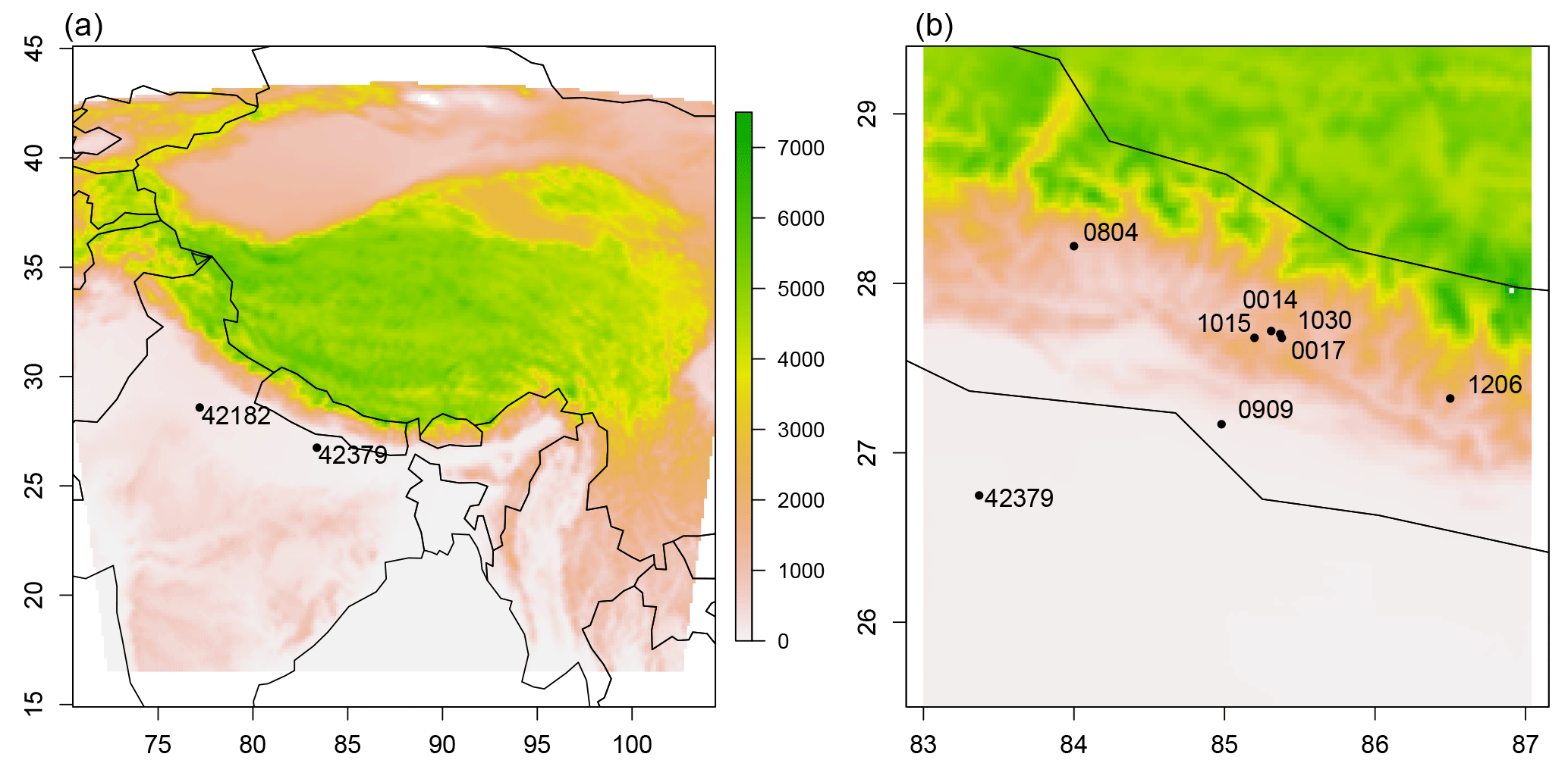
Figure 1Model domains D01 (a) and D02 (b) as used in the WRF and WRF-Chem simulations. Shown are the terrain heights (m) and the locations and station numbers of the measurement sites.
In this study, WRF and WRF-Chem version 3.5.1 are used. In WRF-Chem, we apply the Regional Acid Deposition Model 2 (RADM2) chemistry scheme with the Modal Aerosol Dynamics Model for Europe (MADE)/Secondary Organic Aerosol Model (SORGAM) aerosol module and aqueous-phase chemistry (Community Multi-scale Air Quality model – CMAQ). The combination of RADM2 and MADE has already been applied in many different studies (e.g., Grell et al., 2011). Aqueous-phase chemistry has been switched on as we expect this to be of relevance particularly when simulating aerosols and their wet deposition during the pre-monsoon season. The model domain (D01) covers large parts of the Himalayas, India and Nepal (68–107∘ E, 16–43∘ N, Fig. 1a) at a horizontal resolution of 15×15 km2. The central part of Nepal and the Kathmandu Valley are covered by an additional nested domain (D02) at a horizontal resolution of 3×3 km2 (Fig. 1b). WRF and WRF-Chem are configured with 31 vertical σ levels and with a model top at 10 hPa. The complete set of physics and chemistry options as well as the data used as initial and lateral boundary conditions and emissions used are summarized in Table 1.
Two modifications have been applied to WRF-Chem compared to the standard model version. Firstly, the online calculation of the sea salt emissions in the default WRF-Chem version does not distinguish between ocean and freshwater grid cells (lakes). The model code has been modified to prevent sea salt emissions from small inland lakes. Secondly, currently, there is no calculation of gravitational settling of aerosol particles in WRF-Chem for the chemical mechanism used in this study. Gravitational settling of particulate matter following the method implemented for aerosol particles in the Goddard Chemistry Aerosol Radiation and Transport (GOCART) model (Ginoux et al., 2001) but using the sedimentation velocities calculated by the aerosol module MADE has been implemented into the model code.
(Lin et al., 1983)(Iacono et al., 2008)(Chou and Suarez, 1994)(Hong et al., 2006)(Jiménez et al., 2012)(Grell, 1993; Grell and Dévényi, 2002)(Tewari et al., 2004)(Ackermann et al., 1998; Schell et al., 2001)(Guenther et al., 2006)Wiedinmyer et al. (2011)(Ginoux et al., 2001)(Reynolds et al., 2007)(Janssens-Maenhout et al., 2015)
The model configuration was tested in several sensitivity simulations to find the “best” combination for the study region and is chosen in such a way that allows for simulations over a time period of 6 months and over a relatively large area, and to use the same model setup for the WRF-Chem simulations. Certain aerosol and chemistry options in WRF-Chem are compatible with only specific physics options. Therefore, the physics options for the meteorology-only simulation (WRF) have been chosen in such a way that they are compatible with the chemistry and aerosol scheme in the WRF-Chem simulations.
The main characteristics and the acronyms of the WRF and WRF-Chem simulations analyzed in this study are summarized in Table 2. The reference WRF_ref simulation is a one-way nested meteorology-only (WRF) simulation with two domains (WRF_ref_D01, WRF_ref_D02) (Fig. 1). The time period of January through June 2013 has been chosen to cover the entire measurement period of the SusKat-ABC campaign providing a comprehensive set of meteorological and air pollutant measurements that are well suited for comparison with the model results. Two different nested model simulations have been performed with WRF-Chem (including chemistry and aerosols) for the months of February and May 2013. The month of February has been chosen as an example of a month in the dry season and because the brick kilns, which are in operation then, are thought to be major emitters of black carbon in the Kathmandu Valley. The brick kilns are typically active between December and April, and generally emit continuously throughout the entire day and night. In contrast, May represents a month in the transition phase to the monsoon season (summer) and other sources with more pronounced diurnal cycles become main emitters of black carbon. The first WRF-Chem simulation (WRFchem_ref) has been performed using the global EDGAR HTAP emission inventory v2.2 which is described in more detail in Sect. 2.2.1. For the second WRF-Chem simulation (WRFchem_BC), the EDGAR HTAP emission inventory v2.2 has also been used, but with the black carbon emission values inside the Kathmandu Valley modified to be consistent with estimates based on measurements of black carbon concentrations and mixing layer height (Mues et al., 2017). A detailed description of the emission flux estimates is presented in Sect. 2.2.2.
2.2 Black carbon emission data
2.2.1 EDGAR HTAP
The gridded EDGAR HTAP v2.2 air pollutant emission data (Janssens-Maenhout et al., 2015) combine the latest available regional information within a complete global data set. HTAP uses nationally reported emissions combined with regional inventories. The emission data are complemented with EDGAR v4.3 data for those regions with missing data. The global data set is a joint effort of the US Environmental Protection Agency (US-EPA), the MICS-Asia group, EMEP/TNO, the Regional Emission inventory in Asia (REAS) and the EDGAR group for scientific studies of hemispheric transport of air pollution. The EDGAR HTAP v2.2 data set provides emissions of CH4, CO, SO2, NOx, non-methane volatile organic compounds (NMVOCs), NH3, PM10, PM2.5, BC and organic carbon (OC) on a 0.1∘ × 0.1∘ grid for the years 2008 and 2010 with a monthly time resolution. In the region considered in this study, the emissions are based on data from REAS (Kurokawa et al., 2013) which have a resolution of 0.25∘ × 0.25∘.
Table 3Overview and description of the measurement stations (T indicates temperature, WS indicates wind speed and WD indicates wind direction). DHM indicates the Department of Hydrology and Meteorology of the Ministry of Population and Environment of the Government of Nepal, and IGRA indicates the Integrated Global Radiosonde Archive. MLH indicates mixing layer height.
2.2.2 Observation-based estimates of black carbon emission fluxes for the Kathmandu Valley
In Mues et al. (2017), a method is presented to estimate black carbon emission fluxes for the Kathmandu Valley from mixing layer height data, derived from ceilometer measurements, and black carbon concentrations measured during SusKat-ABC at the Bode station (number 0017) located within the valley (Table 3 and Fig. 1). These estimated emission fluxes are based on measurement data from March 2013 to February 2014 and calculated for each month. The emission estimates are based on the assumptions that (i) black carbon aerosols are horizontally and vertically well mixed within the mixing layer, (ii) the variation of the mixing layer height is only small at night (as frequently observed in the ceilometer measurements used in the study), (iii) the vertical mixing between the mixing layer and the free atmosphere is small (consistent with a stable mixing layer height), and (iv) the horizontal transport of air pollutants into and out of the valley is small (consistent with low nocturnal wind speeds).
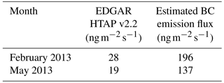
The use of these observationally based black carbon emission fluxes is motivated by the finding that the emission fluxes in the EDGAR HTAP inventory for the Kathmandu Valley are rather small compared to other big cities such as Delhi and Mumbai, where black carbon concentrations are measured that are similar to the black carbon measurements in the Kathmandu Valley. Table 4 summarizes the main differences between the two emission data sets for the Kathmandu Valley for February and May. In the WRFchem_BC simulation, these monthly means were used as black carbon emission fluxes for the grid cells representing the valley. For all other grid cells, the EDGAR HTAP emissions are used. For a more detailed description of the estimation of the black carbon emission fluxes, we refer to Mues et al. (2017).
2.3 Observational data
Measurements of several meteorological parameters and black carbon concentrations are used in this study to evaluate the model performance. These measurements were collected from different sources. An overview of the locations of the measurement stations is presented in Fig. 1 and Table 3; more details on the sources of the measurements are given below.
Table 4Black carbon emission fluxes per month used in the two simulations (WRFchem_ref and WRFchem_BC) for the area of the Kathmandu Valley.
2.3.1 SusKat-ABC field campaign
The SusKat project started with a 2-month long intensive measurement campaign (December 2012 to February 2013), which was extended until June 2013, providing detailed observations of a large number of chemical compounds and meteorological parameters. From December 2012 to June 2013, more than 40 scientists representing nine countries and 18 research groups deployed more than 160 measurement instruments for intensive ground-based monitoring at the urban supersite Bode and a network of 22 additional satellite and regional sites in the Kathmandu Valley and other parts of Nepal (Rupakheti et al., 2018). SusKat-ABC was so far the second largest international air pollution measurement campaign conducted in south Asia, following the Indian Ocean Experiment during 1998 to 1999 (Ramanathan et al., 2001; Lelieveld et al., 2001). SusKat-ABC provides the most detailed air pollution data for the foothills of the central Himalayan region available to date. Hourly data of the following meteorological parameters are available: near-surface temperature, wind direction and speed, relative humidity and precipitation. Furthermore, data on the mixing layer height derived from ceilometer measurements are available (Mues et al., 2017). Black carbon measurements at the Bode site are used in this study for comparison with the WRF-Chem simulations. The black carbon concentrations were measured with a dual-spot aethalometer (Aethalometer AE33, Magee Scientific, USA) (Drinovec et al., 2015) with a time resolution of 1 min. For the model evaluation, all data are used with a time resolution of 1 h calculated as means from the original data. In contrast to the densely built-up center of the Kathmandu Valley, the surroundings of the Bode site are characterized by a mixed residential and agricultural setting in a suburban location with only light traffic and scattered buildings.
Besides Bode, BC concentrations were also measured at Pakanajol, a site near the center of the Kathmandu metropolitan city about 9 km (aerial distance) to the northwest of the Bode site. The BC concentrations at both sites were found comparable in all seasons (Putero et al., 2015, 2018) and have therefore not been used in this study.
2.3.2 DHM measurement data
The Department of Hydrology and Meteorology (DHM) of the Ministry of Population and Environment of the Government of Nepal hosts a network of meteorological stations. Data from five stations within this network were used in order to compare the meteorology simulated with WRF to observations. Hourly data of 2 m temperature and 10 m wind speed and direction were used (Table 3).
2.3.3 ERA-Interim data set
ERA-Interim is a reanalysis data set compiled by the European Centre for Medium-Range Weather Forecasts (Dee et al., 2011). Zonal and meridional wind fields at 500 and 800 hPa are used for comparison with the modeled wind fields, as a general consistency check of the model results. As observations in this region are scarce, the reanalysis data for this region are expected to have larger uncertainties than in regions with a higher coverage of observations.
2.3.4 Radiosonde data
No radiosonde data are available for the Kathmandu Valley, but radiosonde data from the Integrated Global Radiosonde Archive (IGRA) at two locations (Table 3) within the modeling domain D01 can be used for comparison with the model results (Durre et al., 2006, 2008; Durre and Yin, 2008). Both of these two radiosonde stations are located in northern India (Fig. 1), and only one of the stations lies within the highly resolved model domain D02. For station 42182 (New Delhi/Safdarjung), observations are available at around 00:00 and 12:00 UTC between January and June 2013. As launch time of the radiosondes varied, observations for 00:00 UTC also include 23:00 and 01:00 UTC observations, and profiles for 12:00 UTC also include observations for 11:00, 13:00 and 14:00 UTC. In total, 174 profiles were available at around 12:00 UTC and 180 profiles were available at around 00:00 UTC. For station 42379 (Gorakhpur), observations are available only at around 00:00 UTC, which also includes observations at 01:00 and 02:00 UTC due to varying launch times. In total, 77 profiles were available. The processing of the radiosonde observations is further described in Sect. 2.4.
2.3.5 Tropical Rainfall Measuring Mission data
Tropical Rainfall Measuring Mission (TRMM)-based precipitation estimates are used to analyze the geographical distribution of the simulated precipitation fields (Adler et al., 2000). TRMM is a joint mission of NASA and the Japan Aerospace Exploration Agency (JAXA) to measure tropical rainfall for weather and climate research. The TRMM precipitation data are widely used and contributed to improving the understanding of, for instance, tropical cyclone structure and evolution, convective system properties, lightning–storm relationships, climate and weather modeling, and human impacts on rainfall. For the analysis in this study, daily precipitation rates with a spatial resolution of 0.25∘ × 0.25∘ were used (TRMM product 3B-42).
2.4 Evaluation metrics
The model setup chosen in this study is particularly aimed at performing air quality studies in the Kathmandu region. Therefore, a focus in the evaluation of the WRF simulation is on meteorological parameters which are particularly important for air quality. This includes the meteorological parameters temperature, wind speed and direction, the mixing layer height and precipitation. A special focus of the evaluation is on measurement stations in the valley because suitable air quality measurements are only available for this region. For this reason, in particular results for the nested second domain (D02) are shown and discussed. In order to analyze the performance of the WRF model over the target region, the WRF simulation is compared against measurements obtained at surface stations, from radiosondes, as well as satellite products (see Sect. 2.3). For the comparison with the gridded observational data (ERA-Interim), the model results were interpolated onto a regular longitude–latitude grid by applying a simple inverse distance square weighting method. In the case of the station measurements, a station-to-model-grid comparison is done, meaning that the simulation results from the grid cell in which the individual station is located are compared to the station measurements. The model results were saved every 3 h starting at 00:00 UTC. For the model evaluation, only hours with both model and measurement data available were taken into account when producing the figures and the statistics. Here, stations are only considered when they have a data availability of at least 70 % based on hourly data for the time period of interest (except for the mixing layer height) (Table 3).
Radiosonde data are compared to model results in order to evaluate the model's skill in reproducing the observed vertical structure of the atmosphere. Both the observations and model data are averaged over the same pressure bins as well as over the whole period of 6 months. The mean temperature and the median relative humidity over the whole time period and each pressure bin are compared here. The standard deviation indicates the variability over the whole time period within each bin. Model results have only been included in the comparison if observations exist for the respective times.
The statistical metrics used to evaluate the model performance are mean bias (MB) (Eq. 1), root mean square error (RMSE) (Eq. 2) and the Pearson (temporal) correlation coefficient (r) (Eq. 3). The metrics are defined as follows, with N being the number of model and observation pairs, M the model and O the observation values, and σM and σO the standard deviations of modeled and observed values, respectively:
Emery et al. (2001) proposed the idea to use benchmark values derived from several fifth-generation mesoscale regional weather model (MM5) simulations to assess whether model errors in simulating meteorological variables are considered acceptable or not. Specifically, they proposed benchmark values for the temperature MB of ±0.5 K and for the wind speed RMSE of 2 m s−1. Even though these benchmark values were derived from MM5 simulations, they have been also used as references in several studies that evaluate the performance of WRF such as Kumar et al. (2012a) and Zhang et al. (2014).
The precipitation simulated by the model is evaluated against measurements taken at the Bode site and against daily precipitation fields from TRMM (see Sect. 2.3.5). The TRMM data are averaged over domain D02 as an estimate for the precipitation particularly relevant to air pollutant concentrations in the Kathmandu Valley and its surroundings. In the context of air quality, a good hit rate of the occurrence of precipitation events by the model is especially important, rather than the exact representation of the amount of precipitation. The hit rate (H) (Eq. 4), the false-alarm ratio (FAR) (Eq. 5) and the critical success index (CSI) (Eq. 6) (Kang et al., 2007) have been calculated for precipitation at the Bode site and the time period of January to June 2013. These metrics are calculated as follows:
Here, a represents the number of forecast precipitation days (daily sum > 0.5 mm) that were not observed, b represents the number of correctly forecast precipitation days, and d represents the number of precipitation days which were not forecast. Metric H is the percentage of observed precipitation days that are correctly forecast by the model. CSI indicates how well precipitation days were predicted by the model by considering false alarms as well as missed forecasts of precipitation days. In order to compare the two different observations (station measurements and TRMM data), the metrics have also been calculated for the satellite data.
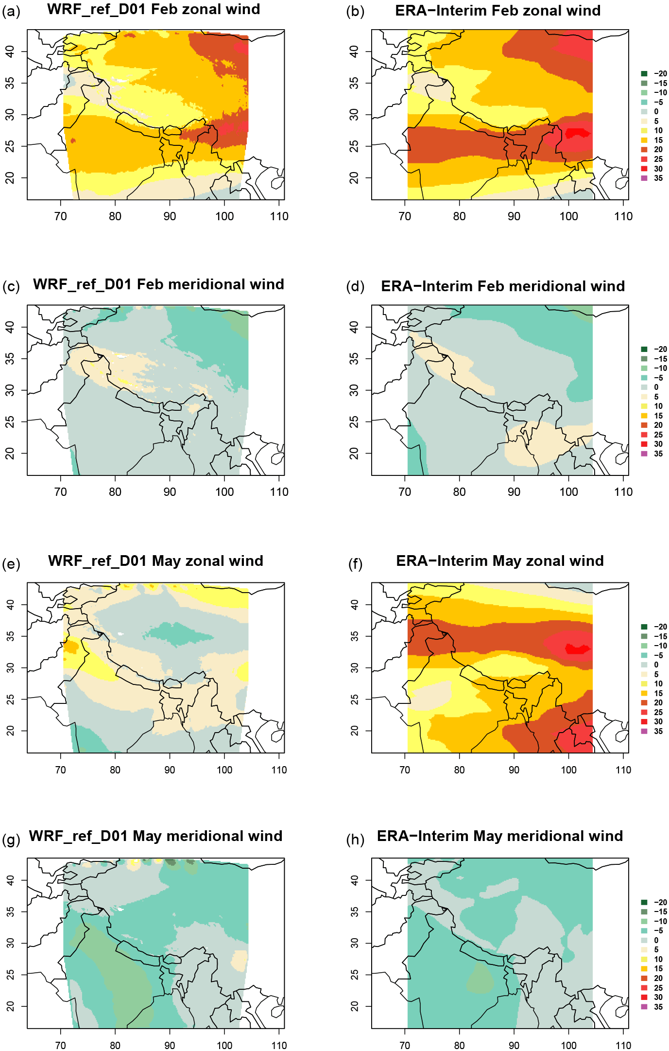
Figure 2Zonal and meridional wind fields in 500 hPa averaged over February and May 2013 for the WRF_ref_D01 simulation (a, c, e, g) and from the ERA-Interim reanalysis (b, d, f, h) in m s−1.
3.1 Evaluation of the WRF model simulation – meteorology
3.1.1 Zonal and meridional wind fields
As a first assessment of the model's performance in reproducing the large-scale wind pattern, the model results are compared to the 500 and 800 hPa wind fields from the ERA-Interim reanalysis. It should be kept in mind that because of the sparsity of available observations in this region, the reanalysis data for this region are expected to have larger uncertainties than in better observed regions. The spatial distributions of the zonal and meridional wind components at 500 and 800 hPa from WRF and the ERA-Interim reanalysis averaged over February and May 2013 are shown in Figs. 2 and S1 (in the Supplement), respectively. The overall pattern of the zonal wind component is qualitatively similar in both data sets for February, with lower values over India in the model simulation. Differences of up to 5 m s−1 are found in the 500 hPa zonal wind component in February, south of the Himalayas, extending in the east–west direction throughout the whole model domain. At 800 hPa, the zonal wind component exhibits differences up to 5 m s−1 in the north of Bangladesh. In May, the zonal wind speed at 500 hPa simulated with the model is much lower compared to ERA-Interim data as shown by the domain-averaged mean bias of 2.9 m s−1. ERA-Interim shows here a stronger westerly wind component. At 800 hPa, the zonal wind is up to 20 m s−1 higher at the bottom of the Himalayas in regards to ERA-Interim data, while the meridional wind is over most of Indian territory up to 5 m s−1 lower than ERA-Interim. The spatial distribution of the meridional wind component simulated by the model is also qualitatively similar to the ERA-Interim fields in both months, with some difference in the southeast of domain D01 in February and over India in May 2013. The domain-averaged mean bias of the monthly mean meridional (zonal) wind fields is 0.1 m s−1 (2.2 m s−1) for February and 0.3 m s−1 (2.9 m s−1) for May, and the spatial correlations of the meridional and zonal wind distributions are 0.9/0.8 and 0.9/0.8 for February and May, respectively.
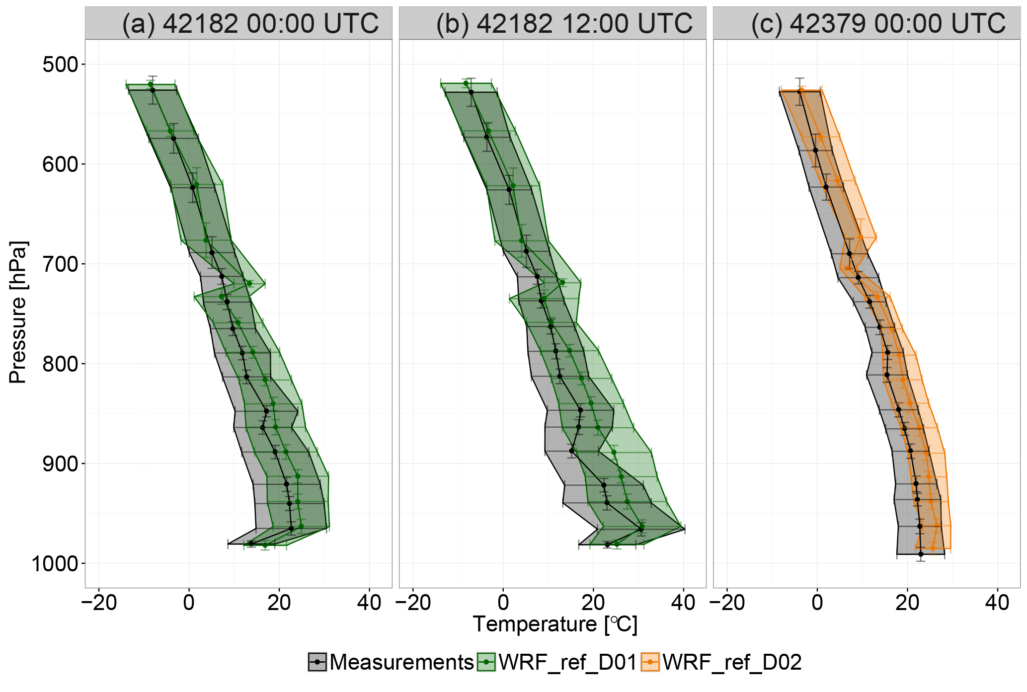
Figure 3Averaged vertical profiles derived from radiosonde data and WRF simulations for temperature (∘C) for the period of January–June 2013. The figures show the results for station 42182 at 00:00 (a) and 12:00 UTC (b) and station 42379 at 00:00 UTC (c). The shaded areas show the standard deviation, indicating the variability over the whole time period within each bin.

Figure 4Averaged vertical profiles derived from radiosonde data and WRF simulations for relative humidity (%) for the period of January–June 2013. The figures show the results for station 42182 at 00:00 UTC (a) and 12:00 UTC (b) and station 42379 at 00:00 UTC (c). The shaded areas show the standard deviation, indicating the variability over the whole time period within each bin.
3.1.2 Vertical profiles
In order to evaluate the ability of the model to correctly represent the vertical structure of the atmosphere, measurements from radiosondes for temperature and relative humidity are compared to the model results (Figs. 3 and 4). This comparison only provides a limited quality check of the model, since there is only a single radiosonde station available within D02. The comparison shows that WRF is able to capture the basic features of the vertical profiles of temperature and relative humidity with the modeled vertical profiles being within the variability estimated by the standard deviation (shaded areas), with the largest differences typically between about 900 and 700 hPa and near the surface.
The measured vertical profiles of temperature at station 42182 show an inversion layer that is also captured by the model. At 00:00 and 12:00 UTC, the observed mean near-surface temperatures are 15 and 24 ∘C; at 960 hPa, they are 22 and 31 ∘C, respectively. The modeled temperatures are about 3 ∘C higher at 00:00 UTC and about 1 ∘C lower at 12:00 UTC compared to the measurements. On average, the modeled mean temperature is overestimated by more than 1 ∘C over the entire column compared with the radiosonde data. The largest differences between model and measurements are up to 6.5 ∘C at 700 hPa (00:00 UTC) and up to 10 ∘C at 890 hPa (12:00 UTC). At 740 hPa, the model shows an underestimation of up to 3 ∘C. At station 42379, the modeled mean temperatures are overestimated by less than 2 ∘C compared with the observations. The standard deviation of the simulated temperature profiles in the lower half of the troposphere is typically around 6 ∘C, which is similar to observed one of around 7 ∘C.
Table 5Statistical overview of the model performance averaged over the time period of January–June 2013 and all available stations based on 3-hourly data. Station measurements are included in the statistics if the data availability is over 70 % (Table 3).
The measured vertical relative humidity profiles are well reproduced by the model within the first five vertical layers with the model bias at each model level ranging between −4 and 4 %. Between 900 and 740 hPa, the model overestimates relative humidity by up to 20 %. As for temperature, the model reproduces the observed standard deviation of relative humidity quite closely at all heights investigated, with the standard deviation ranging from 16 % at surface up to 25 % at about 570 hPa.

Figure 5Time series of measured, simulated (WRF_ref_D02) and simulated but height-corrected (WRF_ref_D02_corr) daily mean 2 m temperature (∘C) during January–June 2013 at stations 0804 (a), 1015 (b), 0014 (c), 0017 (d) and 1206 (e). The tables in the subfigures give the temporal correlation and the mean bias between simulated and measured values (∘C).
3.1.3 2 m temperature
The daily mean 2 m temperature increases during the simulation period at all stations shown in Fig. 5, from about 5–10 ∘C in January to 20–30 ∘C in June, which is also shown by the model (WRF_ref_D02). While the observed temporal evolution of the daily mean near-surface temperature is well reproduced by the model (correlation above 0.9; Fig. 5), the absolute values are systematically over- or underestimated at several stations. The mean bias for WRF_ref_D02 ranges between −1.9 and 2.2 K (Fig. 5). This MB is larger than the benchmark value of ±0.5 K from Emery et al. (2001). Here, it should be noted that at several stations the over- or underestimation of measured temperature is associated with a difference between the actual elevation of the measurement station and the elevation of the model grid cell the station is located in. For example, at station 1206, the elevation of the grid cell in the domain D02 is 149 m lower than the elevation of the measurement station (1720 m); given a typical atmospheric vertical temperature gradient of 6–7 K km−1, one would expect a bias of about 1 K, which is close to the actual mean temperature bias of 0.8 K. In order to correct for the temperature biases caused by differences in elevation, a height correction has been applied to the model data by linearly interpolating the modeled vertical temperature profile to the elevation of the measurement station. For the stations, the mean bias was reduced by 1 K (station 0014) to 0.2 K (station 1206) (Fig. 5) when considering this height correction. Table 5 summarizes the statistics averaged over all available stations and the whole simulated time period based on 3 h data. On average, the model overestimates the observed mean temperatures by 0.7 K, which is slightly larger than the benchmark value from Emery et al. (2001) but still suggesting that the model performance is acceptable given the challenging topography of the Himalayas. The mean daily minimum and maximum temperatures are overestimated by 1 K and underestimated by 0.5 K, respectively. The main features of the average diurnal cycle of the 2 m temperature (Fig. 6) are reproduced by the model but the daily temperature amplitudes (difference between the daily minimum and maximum temperature) are often smaller in the model simulation than in the measurements. This is mainly caused by a high bias in the simulated values in the morning hours. In contrast, the daily variability of the 2 m temperature shown by the 25th and 75th percentiles in Fig. 6 is reproduced quite well by the model.
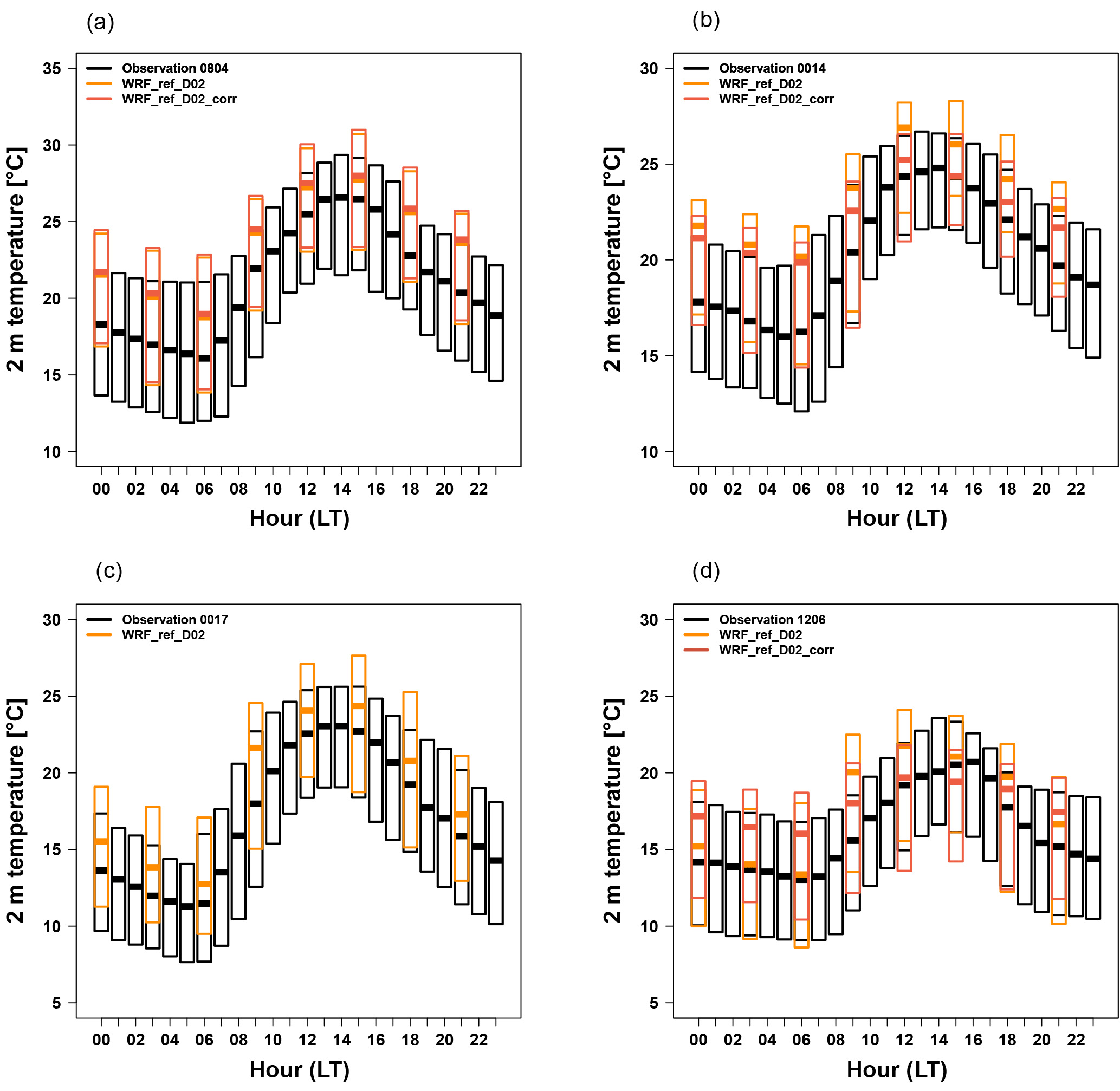
Figure 6Diurnal cycle of the measured, simulated (WRF_ref_D02) and simulated but height-corrected (WRF_ref_D02_corr) 2 m temperature (∘C) for the period of January–June 2013 as a boxplot (showing the median, the upper and lower quantiles) at stations 0804 (a), 0014 (b), 0017 (c) and 1206 (d).
The temperature biases found at stations in the present study are in the same range as the ones found in other regions with WRF (Zhang et al., 2013, 2016; Mar et al., 2016; Kuik et al., 2015), particularly when considering that the reported 2 m temperature biases in these studies tend to be higher in mountainous terrain than in other regions. For example, Zhang et al. (2016) found a mean bias in the 2 m temperature of −1.5 to 1 K at stations in east Asia, while at single stations the mean bias can range between −5 and +5 K in January and July 2005, respectively. Kuik et al. (2015) found a good agreement between WRF-Chem simulations for south Africa and ERA-Interim reanalysis data 2 m temperature in 2010 (mean bias 0.4 and −0.03 K, spatial correlation 0.93 and 0.91, for September and December, respectively). Mar et al. (2016) found that the spatial variability in measured 2 m temperature is well reproduced by WRF-Chem in all seasons in 2007 over Europe with values of the absolute mean bias of generally less than 1 K. Both Mar et al. (2016) and Zhang et al. (2013) found the largest biases in 2 m temperature in the Alps. Mar et al. (2016) describes an overprediction by more than 1 K in this region, whereas Zhang et al. (2013) found a cold bias of −5 to −2 K.
3.1.4 10 m wind speed and direction
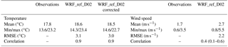
The wind speed has an essential impact on the horizontal transport of pollutants. For example, low wind speeds favor an accumulation of pollutants close to their sources, whereas higher wind speeds lead to the transport of pollutants away from their source. The average measured wind speed over all stations and over the 6 months based on hourly data is 1.7 m s−1 (Table 5), which is overestimated by the model by 1 m s−1. The averaged RMSE value over all stations of 2.2 m s−1 is close to the benchmark value of 2 m s−1 proposed by Emery et al. (2001). In fact, at most individual stations, the RMSE values are within the benchmark range. At individual stations where wind speed data are available, the biases range between 0 and 1.7 m s−1. The temporal correlation coefficient of hourly wind speed is on average 0.4 with a range of 0.1 to 0.6 at these individual stations (Table 5). The overestimation in wind speed in the WRF_ref_D02 simulation can probably be attributed to a large extent to an overestimation of the maximum wind speed during daytime, which is on average biased positively by 2 m s−1. In contrast, the daily minimum wind speed is close to the observation (MB of 0.2 m s−1) (Table 5). This is also clearly seen in the frequency distributions of the wind speeds (Fig. S1), which typically have a much broader distribution with higher wind speeds and a maximum shifted to larger values for the model compared to the observations.
This performance of WRF in reproducing the observed mean 10 m wind speed is consistent with biases reported in the literature, especially when considering stations in mountain regions. For example, Mar et al. (2016) found an overestimation of the modeled wind speed over Europe, especially during winter and fall with a bias of 2 m s−1 and more. Regions with a larger bias include the mountain region of the Alps, indicating the challenges of simulating wind accurately over complex terrain. The temporal correlation of the modeled 10 m wind speed in Europe is typically above 0.7 but lower (0.4–0.6) over the Alps and close to the Mediterranean (Mar et al., 2016), which is still higher than the correlation found at some stations in this study. Zhang et al. (2013) describe a significant overprediction at almost all sites investigated in Europe (MB of 2.1 m s−1) with the largest biases over several countries in low-lying coastal areas and over the Alps as well as the Carpathian Mountains. They argue that these results indicate the difficulty of the WRF model in simulating wind patterns and mesoscale circulation systems (such as sea breeze and bay breeze) and their interaction with land over complex terrain. Furthermore, they state that this high bias in 10 m wind speed can be mainly attributed to a poor representation of surface drag exerted by the unresolved topography in WRF. Yver et al. (2013) tested different planetary boundary layer (PBL) schemes in their model setup and also found an overestimation of wind speed at stations in California in all cases, although of different magnitude (about 0.5 to 3 m s−1). Zhang et al. (2016) found a significant overprediction of 10 m wind speed at stations in east Asia with a mean bias of 1.9–3.1 m s−1.
An evaluation of the 10 m wind speed and especially the wind direction at the individual measurement stations (not shown) strongly suggests that these parameters are highly dependent on the stations' locations and the topography of their surroundings, especially in mountain areas. The measurements at some of these sites are therefore probably only representative of a rather small area around the station. Because of the complex topography in this region, a horizontal resolution of 3×3 km2 is too coarse to represent the near-surface wind at sites strongly influenced by small-scale features such as individual mountains. Therefore, the main focus of the evaluation of the 10 m wind is on the Kathmandu Valley. The Kathmandu Valley, with a diameter of about 30 km, is starting to be large enough to be resolved at the model resolution of 3×3 km2. The relatively flat valley floor further facilitates a comparison of the 3×3 km2 model grid cells with observational data, as measurements inside the valley are expected to be less influenced by small-scale topography than at most stations outside the valley.
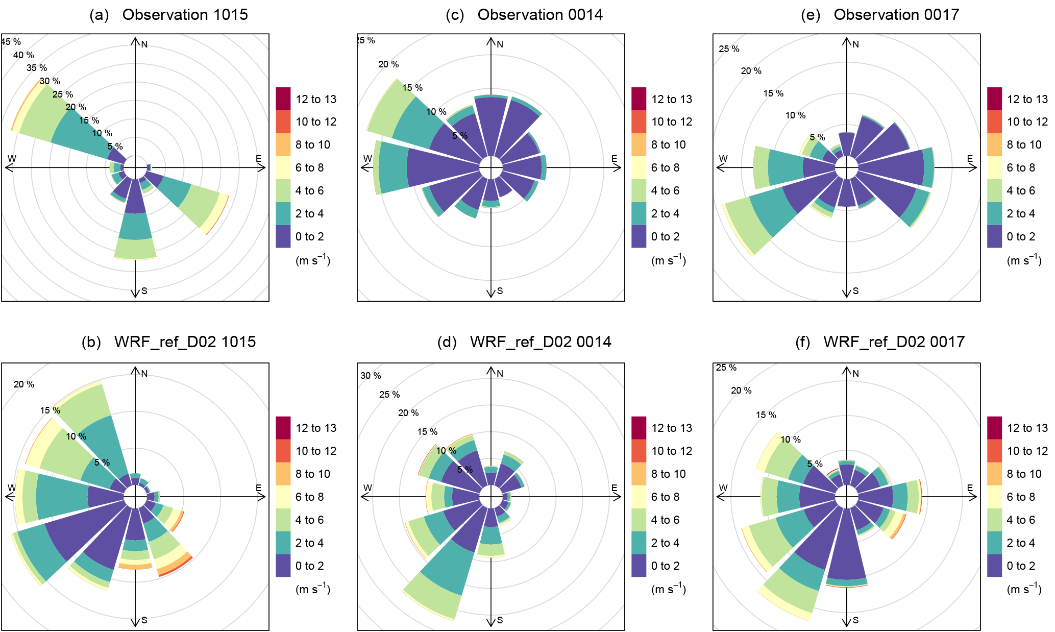
Figure 7Wind roses based on measured and simulated (WRF_ref_D02) wind speed and direction at four stations – 0018 (a, b), 1015 (c, d), 0014 (e, f) and 0017 (g, h) – in the Kathmandu Valley for the time period of January–June 2013 based on 3 h data. Shown are wind speed (color) (m s−1) and the frequency of counts by wind direction (%).
The frequency distribution of wind speed per wind direction based on 3-hourly data for the whole simulation period is shown in Fig. 7 as wind roses for all available stations in the valley. The main wind directions in the east of the valley (station 1015) are north–northwest, east–southeast and south, with wind speeds of typically up to 6 m s−1. In contrast to the observations, the model shows wind directions from north–northwest to south–southeast. Wind speeds are similar as observed. The main wind direction at stations in the west of the valley (0014 and 0017) is less clearly dominated by particular sectors more than that in the east of the valley but rather characterized by predominately westerly winds. This pattern is reproduced by the model, although the wind speed is generally overestimated. The observed diurnal cycle of wind speed at the Bode station (Fig. 8a) shows very low median values between 0 and 1 m s−1 during the night and a maximum median wind speed during daytime of about 4 m s−1. As discussed before, the low wind speed during night is well reproduced by the model but the maximum wind speed during daytime is overestimated. The main wind direction during nighttime is from the east–southeast (around 100∘) in the observations (Fig. 8b), while it is from around 180∘ in the model. For such low wind speeds, however, the measured wind direction is expected to be affected by small-scale dynamics such as turbulence and thus not expected to be directly comparable to a 3×3 km2 model grid cell. In the transition phase from low to high wind speed during morning hours (09:00–11:00 LT) and from high to low wind speed in the evening (19:00–21:00 LT), the model does not reproduce the wind direction correctly. In contrast, the main wind direction during daytime is west–southwest (around 250∘) which is reasonably well reproduced by the model.
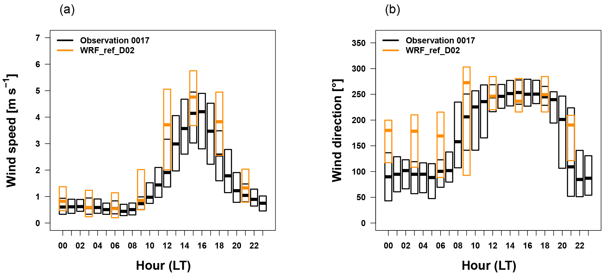
Figure 8Diurnal cycle of the measured and simulated (WRF_ref_D02) wind speed (m s−1) (a) and wind direction (∘) (b) for the period of January–June 2013 as a boxplot (showing the median, the upper and lower quantiles) at the Bode station.
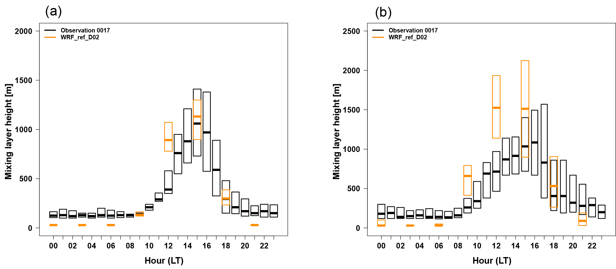
Figure 9Diurnal cycle of the mixing layer heights (m) as a boxplot (showing the median, the upper and lower quantiles) as diagnosed by the WRF model (WRF_ref_D02) and as determined from ceilometer measurement data at the Bode site for the period of January–February (a) and March–June 2013 (b).
3.1.5 Mixing layer height
A key parameter for air quality is the depth of the mixing layer which is a part of the planetary boundary layer and characterized by a strong gradient in parameters such as potential temperature and aerosol concentration, and by an unstable layer and strong mixing due to turbulence during daytime and a rather stable layer during nighttime. Thus, the mixing layer has an important impact on the dispersion or accumulation of pollutants at the ground level. In the WRF model, the mixing layer height is a diagnostic variable which is calculated based on the Richardson number (Hong et al., 2006). The model output is compared to the values derived from ceilometer measurements obtained during SusKat-ABC (Mues et al., 2017). In Fig. 9, the diurnal cycle of the mixing layer height calculated from data covering the two time periods (January–February and March–June 2013) is shown for the model (WRF_ref_D02) in comparison with the ceilometer data. Both model and observations show a distinct diurnal cycle with low mixing layer heights during the night and morning hours and higher values during the day. While the lowest measured nocturnal values are around 160 m in January–February and around 200 m in March–June, the modeled values typically go down to less than 50 m in all seasons. The maximum mixing layer height values are measured at around 16:00 LT in the afternoon with a median of 1060 m in winter and 1053 m in the pre-monsoon season. The simulated values are higher during the day, with a median of 1132 m at 15:00 LT in winter and of 1512 m during the pre-monsoon season. These over- and underestimations of the maximum and minimum in the diurnal cycle are also shown for individual months, for instance, a high/low bias for the maximum/minimum mixing layer height of +244/−76 m in February and +280/−122 m in June. The mean bias in the modeled maximum/minimum diurnal mixing layer height is +81/−32 m in January–February and +438/−372 m in March–June.
A similar pattern was also found by Kuik et al. (2016) for WRF-Chem simulations over Germany in summer, with a mean bias of −113 m for the daily minimum and 287 m for the daily maximum mixing layer height. This is also in agreement with Singh et al. (2016), who showed an overestimation up to 204 m in February 2012, and up to 584 m in March 2012 of the modeled boundary layer height predicted at a measurement site in the central Himalayas.
Furthermore, the simulated diurnal cycle of the increase in mixing layer height during daytime is shifted by about 2 h to earlier times compared to the measurements. During the day, convection is an important process for determining the mixing layer height. A premature onset of convection found in many models is a long-standing issue and has been identified in numerous previous modeling studies, including studies with WRF (e.g., Pohl et al., 2014).
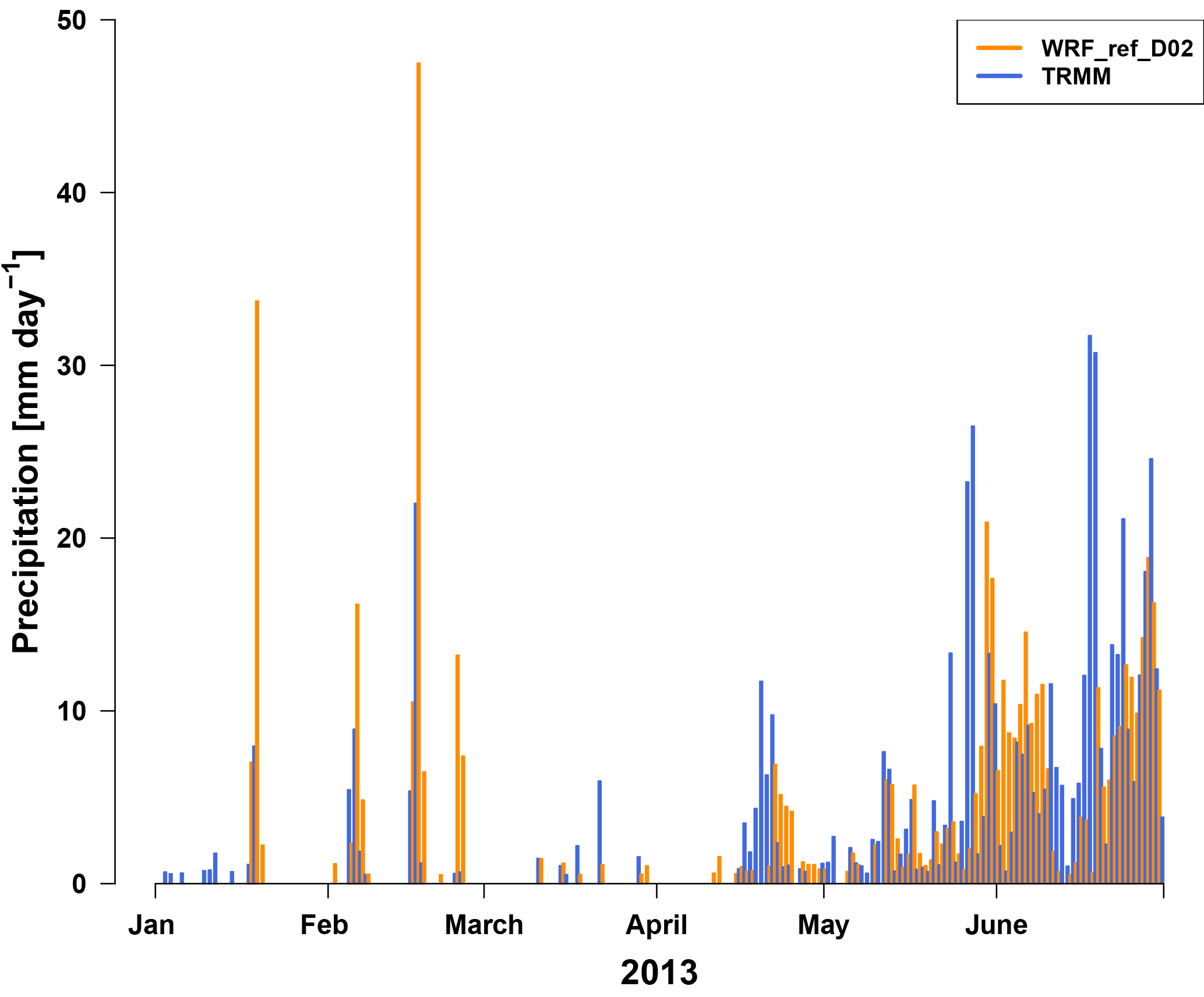
Figure 10Time series of precipitation (mm day−1) averaged over the domain D02 from WRF_ref_D02 and TRMM per day for January–June 2013 based on daily sums.
3.1.6 Precipitation
A good representation of the precipitation in the model is important for the calculation of wet deposition of air pollutants such as particulate matter including black carbon. The domain-averaged daily precipitation totals from the model (WRF_ref_D02) and TRMM are shown as a time series in Fig. 10. The near absence of strong rain events in the dry season (January through April) is reproduced well by the model, and also the timing of the single rain events between January and March is reproduced relatively well, although the total amount of precipitation is overestimated by the model. This overestimation is particularly strong during the dry season, as can also be seen for February in Fig. 11. Here, the strongest overestimation of precipitation by the model is seen in the northern part of Nepal and seems to be related to the particularly high and steep orography in this part of the country. The transition to and start of the rainy season in late April/early May as seen in the TRMM data are reproduced reasonably well by the WRF simulation. The geographic distribution of the observed average precipitation rates during the rainy season which is shown in Fig. 11 for May shows rain rates between 6 and 15 mm day−1 particularly over Nepal, and rain rates between 0 and 5 mm day−1 over northern India and the part of the Tibetan Plateau covered by model domain D02. This is qualitatively well reproduced by the model.
Table 6Number of observed and forecast precipitation days (days with sum of precipitation > 0.5 mm day−1) during the period of January–June 2013. Yes/yes – both data sets have a precipitation day at the same time; yes/no – first data set has a precipitation day, second does not; no/yes – first has no precipitation day, second does; no/no – both do not have a precipitation day. FAR – false-alarm ratio, CSI – critical success index, H – hit ratio.
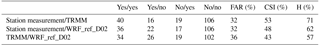
The statistics summarized in Table 6 represent the skill of the model (WRF_ref_D02) to reproduce precipitation events at a single station in the valley (Bode). It shows that 62/57 % (H) of the observed precipitation days are correctly captured by the model when using the Bode station measurements and the TRMM data, respectively, as reference data. The ratio of days when precipitation was present in the model data but not measured relative to all forecasted precipitation days (FAR) is relatively high: 32 % for the station measurements and 36 % for the TRMM data. Other than the hit rate, the CSI also considers false alarm and missed forecast, but it is not influenced by correctly forecast no-precipitation days. The CSI score indicates that 48 % of the forecast and observed precipitation days are correct. When using the TRMM data as observational reference, the score is a bit smaller (43 %). Hit rate and CSI are both lower for the model if considering TRMM as reference. Differences between the two observational data sets (station measurement and TRMM data) are shown in Table 6. The hit rate for the station measurements and the TRMM data (station measurement/TRMM) indicates that 71 % of the measured precipitation days at the Bode station are also visible in the TRMM data. The differences obtained when using the two different observational data sets also show the uncertainties and limitations particularly of the TRMM data for this kind of comparison. Since some of the precipitation events can be rather localized (e.g., convective rain) and can thus not be expected to be fully reproduced by a 3×3 km2 model simulation, they might also be missed in the rather coarse spatial and temporal (satellite overpass times) resolution satellite data.
3.1.7 Sensitivity of temperature and wind speed to nudging and land use data
In order to test that the simulated large-scale circulation does not drift or deviate from the observed synoptic condition, a sensitivity simulation in which a grid nudging technique was employed for horizontal winds, temperature and water vapor above boundary layer has been performed. In this simulation, we obtained similar results as in the reference simulation; for example, the RMSE of temperature is 3.0 K using the nudging approach compared to 3.1 K in the reference run. The model performance for wind speed does not change. In the upper troposphere, the differences in the simulated meteorological variables in the reference and the sensitivity runs were not statistically significant, suggesting that the WRF model results in this altitude range are mostly driven by the prescribed boundary conditions. In a second sensitivity simulation, we have analyzed the impact of using MODIS land use data instead of the default USGS data set. In this simulation, the impact of using the MODIS data together with applying the nudging technique on WRF results is tested for temperature and wind speed parameters. As in the first sensitivity simulation, the RMSE of temperature does not deviate much from the one obtained from the reference simulation, i.e., using USGS land use data and no nudging, leading to a RMSE of 2.9 K compared with 3.1 K in the WRF_ref_D02 simulation. In contrast to temperature, the model performance for wind speed worsens with a RMSE of 3.2 m s−1 and an average correlation coefficient of 0.21. Since the relatively small number of measurement stations in the evaluation domain might not be representative of the whole domain, we have also compared the results from the sensitivity simulations with the reference simulation. When applying the nudging technique, the domain-averaged mean bias between the sensitivity and the reference simulation is −0.03 K for temperature and 0.08 m s−1 for wind speed. For the MODIS land use sensitivity simulation, the domain-averaged mean bias when compared to the reference simulation is 0.08 K for temperature and 0.2 m s−1 for wind speed. This suggests that the changes in temperature and wind speed when applying the nudging technique and using the MODIS land use data set are rather small and not expected to be important factors in explaining the differences between the model results and observations found.

Figure 11Monthly mean precipitation rates in mm day−1 for domain D02 from WRF_ref_D02 (a, c) and TRMM (b, d) for February and May 2013.
3.2 WRF-Chem model simulations of black carbon
3.2.1 Results from the WRFchem_ref and WRFchem_BC model simulations
Two WRF-Chem simulations have been performed with an identical model configuration but using different black carbon emissions. The WRF-Chem reference simulation uses the EDGAR HTAP emissions (WRFchem_ref); the second simulation uses the same emission data but with black carbon emission fluxes over the Kathmandu Valley replaced by emission estimates based on SusKat-ABC measurements (WRFchem_BC) (see Sects. 2.2.1 and 2.2.2 for details on the emission data sets). The black carbon emission fluxes used in both WRF-Chem simulations are shown in Fig. 12.
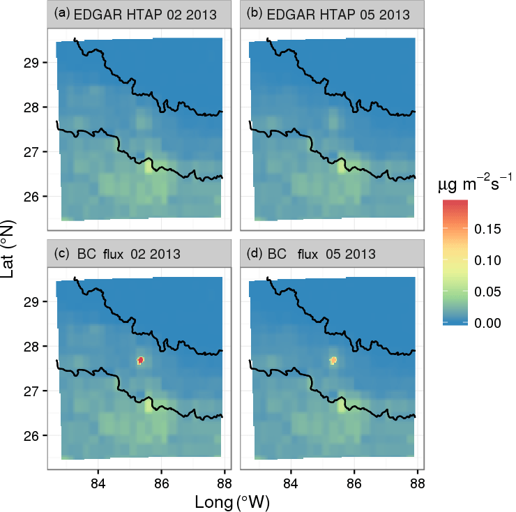
Figure 12Black carbon emission flux used for the WRFchem_ref_02/05_D02 (a, b) and WRFchem_BC_02/05_D02 (c, d) simulations for February (left) and May 2013 (right) in .
Monthly mean black carbon concentrations measured in the Kathmandu Valley at the Bode station are 27 µg m−3 in February 2013 and 11 µg m−3 in May 2013. These values are strongly underestimated in the reference simulation WRFchem_ref_D02 (using EDGAR HTAP emissions), which average only 3 µg m−3 (89 % underestimate) in February and 2 µg m−3 (82 % underestimate) in May. The WRF-Chem sensitivity simulation using the black carbon emission fluxes inside the Kathmandu Valley estimated from observations (WRFchem_BC_D02) shows significantly reduced biases, averaging 12.5 µg m−3 (54 % low bias) in February and 6 µg m−3 (45 % low bias) in May. These results from WRFchem_BC_D02 are in much better agreement with the measurements at the Bode site, even though black carbon is still underestimated by the model. The improvement of the simulated black carbon concentrations when using the observationally based estimated fluxes can also be seen in the time series of daily mean black carbon concentrations (Fig. 13). Measured daily black carbon concentrations reach values of up to 35 µg m−3 in February and up to 28 µg m−3 in May, with a pronounced variability within the same month (e.g., 2–5 May vs. 6–8 May). The daily mean black carbon concentrations from the reference simulation WRFchem_ref_D02 are below 5 µg m−3 in both months. The differences between the two months as well as the large daily variability are not reproduced by the reference simulation. In contrast, the time series of the WRFchem_BC_D02 sensitivity simulation shows values of up to 20 µg m−3 in February and up to 8 µg m−3 in May. In addition, the observed differences between February and May as well as the daily variability are better reproduced than in the reference simulation WRFchem_ref_D02. In order to compare the spatial variability of the simulated black carbon concentration in the valley, also the daily mean concentrations simulated in the grid cells with the highest and lowest values of all neighboring grid cells of the Bode grid cell are shown in Fig. 13. The spatial variability of the simulated black carbon concentration is higher (in absolute and in relative terms) in the WRFchem_BC_D02 simulation compared to WRFchem_ref_D02. This figure also shows that the grid cell with the Bode station is not an outlier but generally at the upper end of the range of minimum and maximum concentrations of its neighbors.
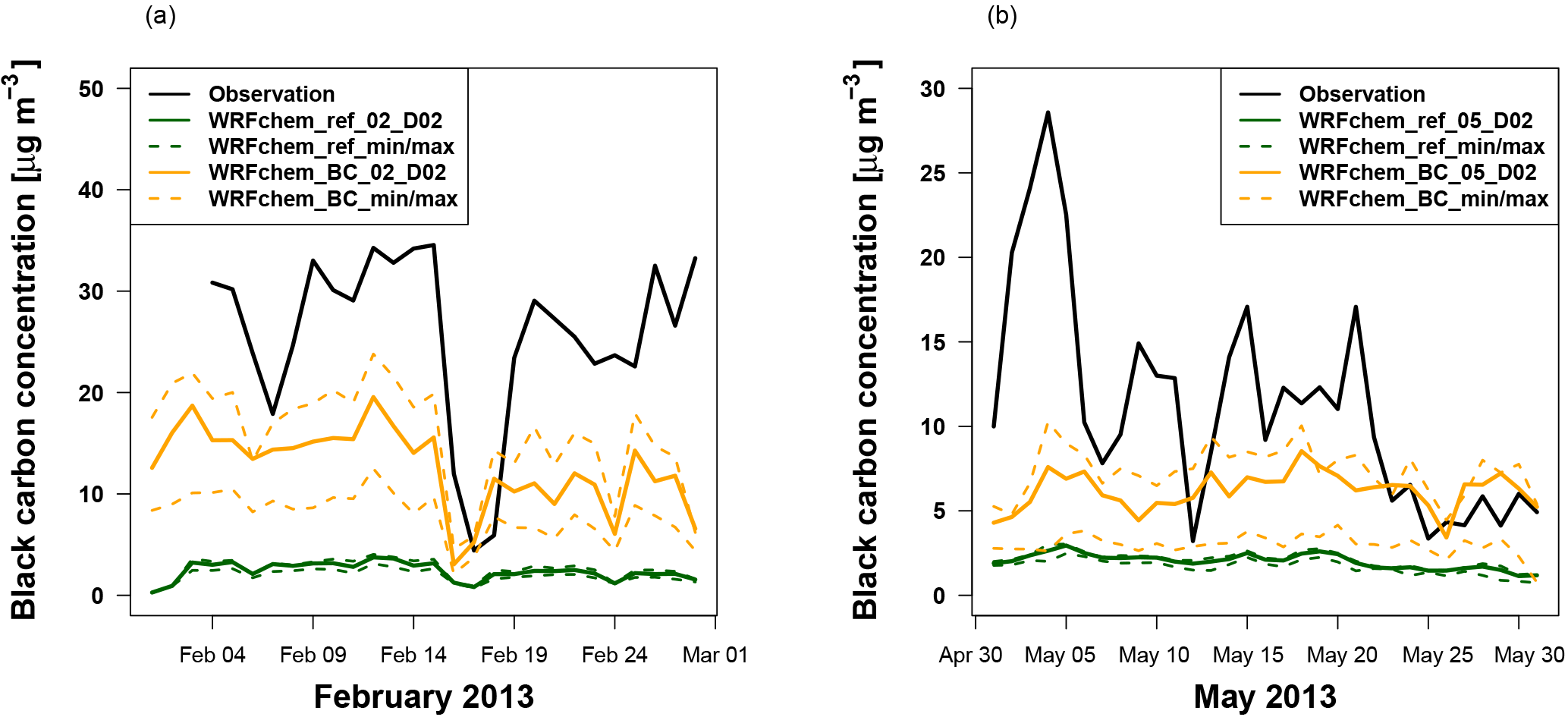
Figure 13Time series of daily mean measured and simulated (WRFchem_ref_02/05_D02, WRFchem_BC_02/05_D02) black carbon concentrations (µg m−3) at the Bode station for February (a) and May (b) 2013.
The histogram of the measured hourly black carbon concentrations (Fig. 14) shows values of up to 90 µg m−3 and a maximum of the distribution between 0 and 10 µg m−3. These values of the measured frequency distribution are not reproduced by the reference simulation WRFchem_ref_D02, in which the black carbon concentrations range only between 0 and 6 µg m−3 with a maximum frequency between 1 and 1.5 µg m−3. The histograms of the WRFchem_BC_D02 simulation for February and May show a wider frequency distribution compared to the reference simulation WRFchem_ref_D02 with maximum concentrations of up to 40 and 20 µg m−3, and maximum frequencies in the interval 0 to 10 µg m−3 and around 5 µg m−3 (in February and May, respectively).
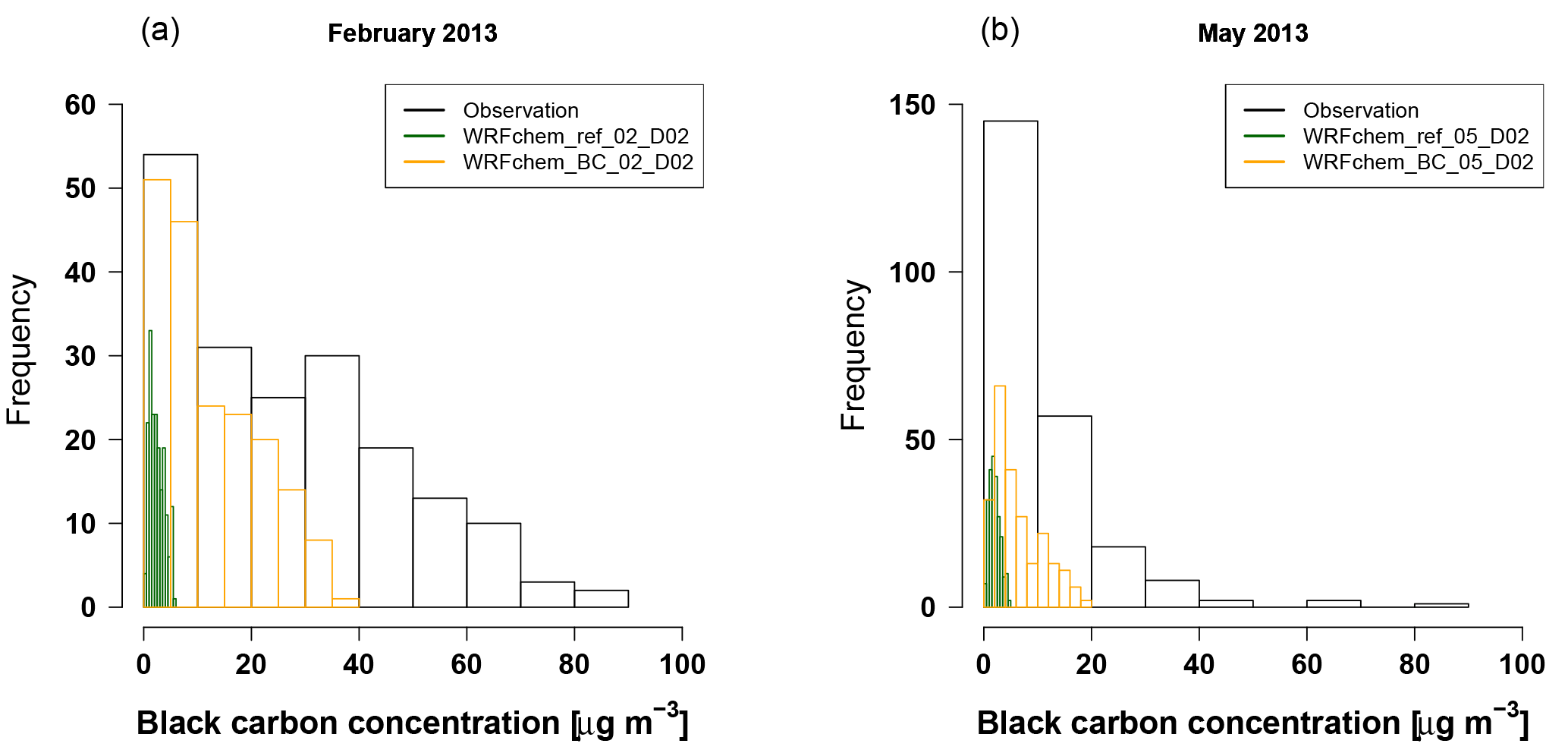
Figure 14Black carbon concentrations at the Bode site, measured and simulated with WRF-Chem for February 2013 WRFchem_ref_02/05_D02 (a) and for May 2013 WRFchem_ref_02/05_D02 (b) as a histogram calculated from the 3 h values.
The pollution roses in Fig. 15 show the measured and simulated black carbon concentrations coinciding with each specific wind direction at the Bode station and the frequency of the occurrence of the corresponding wind direction in percent. The figure shows that the observed main wind direction in February is from the west and west–southwest, but high black carbon concentrations are found for all wind directions. Simulated main wind directions span a wider range than in the observations (west–northwest, southwest and south) but the model reproduces the observation that high black carbon concentrations are found independent of the actual wind direction. In May, the observed main wind direction is from the west (and slightly north and south of west), and the highest concentrations are measured for winds from the north and east–southeast (Fig. 15d). Again, the model does not fully reproduce the main wind directions (here northwest to south) and underestimates black carbon concentrations in all wind directions.
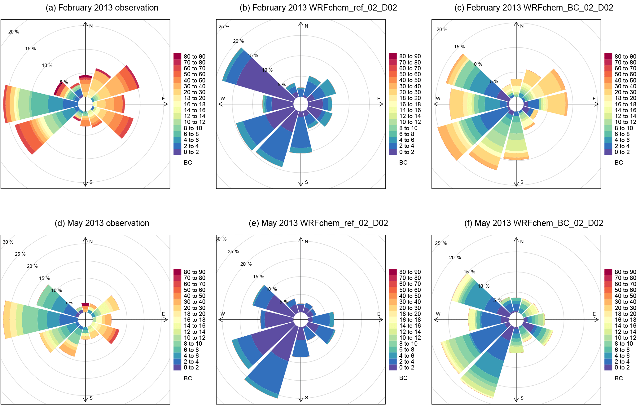
Figure 15Pollution rose for black carbon at the Bode site calculated from the measured and simulated (WRFchem_ref_02/05_D02 and WRFchem_BC_02/05_D02) 3 h values of black carbon, wind speed and direction in February (a, b, c) and May (d, e, f) 2013. The figures represent the black carbon concentrations which coincide with a certain wind direction at the station and the frequency of occurrence of the wind direction in percent.
These findings strongly suggest that the EDGAR HTAP emissions of black carbon in the valley are underestimated and that there is a need for further improvements of the local emissions in the Kathmandu Valley. Despite this improvement in the simulated black carbon concentrations in the Kathmandu Valley when using the black carbon emission fluxes estimated from observations, the measured concentrations are still significantly underestimated by the model.
3.2.2 Discussion of the observation-based emission estimates for black carbon
Two possible reasons for the abovementioned underestimation of the observed black carbon concentrations in the WRFchem_BC_D02 simulation are an overestimation of the dispersion of the black carbon aerosols away from the ground and too small observation-based black carbon emission estimates. Even though the model tends to overestimate the observed near-surface wind speed, the model bias of about 1 m s−1 is not expected to be large enough to explain the large differences in simulated and observed black carbon concentrations through an overestimated horizontal dispersion. The observed and simulated mixing layer heights (Fig. 9) are quite similar, suggesting that the model is able to produce a reasonable vertical dispersion. Furthermore, particularly at nighttime, the smaller-than-observed simulated mixing layer height would rather lead to an overestimation of the observed black carbon concentrations by the model. This suggests that biases in the modeled dispersion (horizontal and vertical) alone are unlikely to be able to explain the large differences in modeled and observed black carbon levels. This, in turn, suggests that the top-down emissions determined by Mues et al. (2017) based on the observed black carbon concentrations and mixing layer heights might be underestimated – despite the fact that they are several times as high as the values in the state-of-the-art EDGAR HTAP v2.2 data set (for further discussion of the observation-based emission estimates for BC in comparison with available emission inventories, we refer to Mues et al., 2017).
There are various possible reasons why the top-down emissions derived from measurements at the Bode station might be underestimated or not fully representative of the entire Kathmandu Valley as assumed in the sensitivity study WRFchem_BC. One main reason is that the Bode station is not located in the urban center. Thus, throughout most of the year, during the months when the brick kilns near Bode are not operating, several important urban emission sources such as traffic, cooking and open burning of trash might be underestimated due to applying the top-down method to determine the black carbon emission flux based on the semi-urban Bode site data. Future development of high-resolution (e.g., 1×1 km2) emission data sets (Sadavarte et al., 2018) may help to resolve this possible discrepancy. An important first step for such work is the measurements of various fuel-based emission factors obtained during the Nepal Ambient Monitoring and Source Testing Experiment (NAMaSTE, Jayarathne et al., 2018).
The other main possible reason for the top-down emissions to underestimate actual emissions is that the method currently only considers sources that are active at night, when the mixing layer height is stable and the increase in black carbon concentrations can be directly attributed to emissions during that time period. It is assumed that the average emissions during the rest of the day are the same as during this period. This can lead to either an over- or underestimation, depending especially on the extent to which the morning food preparation and rush hour traffic occur during the period of the stable nocturnal boundary layer. It is possible that the contribution of black carbon sources which are mainly active during daytime, after the nocturnal boundary layer begins to break up, exceeds the nighttime emissions. Since the daytime-specific emissions such as rush hours throughout much of the year and the generally heavier daytime traffic are not taken into account by the top-down computation, this could lead to an underestimation in the black carbon emission fluxes. This is consistent with the statement by Mues et al. (2017) that the top-down emission estimate is “likely a lower bound” and thus strongly supports the indication of an underestimation of the values in current emission data sets. Unfortunately, no technique has yet been found to apply the top-down method for the full diurnal cycle in the situation of the Kathmandu Valley, so it will be left to emission inventory developers to improve their estimates based on updated emission factors and activity data for the region, in order to hopefully determine what is missing according to the top-down analysis.
Despite that offset that is apparently due to the emissions, the temporal correlation coefficient between daily data of the WRFchem_BC_D02 results and the Bode observations is relatively high (0.7) in February, while it is much lower (0.2) in May 2013. There are likely two factors that contribute to this difference. Firstly, in May, the day-to-day variability of the emission strength from different sources can expected to be higher because brick kilns, which emit black carbon relatively constantly throughout the day and night, are no longer running, and emission sources with a much clearer diurnal cycle like cooking, traffic and trash burning take on a greater relative importance. Secondly, the meteorology in May is more difficult to simulate than that in February as convective precipitation becomes more frequent. The correct simulation of the occurrence of daily precipitation events is particularly important in this context. Although the transition from the dry season in winter to the wet season in summer is captured well by the model, there are several days when precipitation was observed and not simulated in the model and the other way around (Table 6), which has an important impact on the simulated day-to-day variability of black carbon. In addition to particles being removed by wet deposition, also certain emission sources such as burning of trash and biomass, can be affected by precipitation.
An evaluation of the simulated meteorology with the WRF model over south Asia and Nepal with a focus on the Kathmandu Valley for the time period of January to June 2013 is presented in this study. The model evaluation is done with a particular focus on meteorological parameters and conditions that are relevant to air quality. The same model setup is then used for simulations with the WRF model including chemistry and aerosols (WRF-Chem). Two WRF-Chem simulations have been performed: a reference simulation using emissions from the state-of-the-art EDGAR HTAP v2.2 database along with a sensitivity study using modified, observation-based estimates of black carbon emission fluxes for the Kathmandu Valley. The WRF-Chem simulations have been performed for February and May 2013 and are compared to black carbon measurements in the valley obtained during the SusKat-ABC campaign.
The ability of the model to reproduce the large-scale circulation is tested in this study by comparing the simulated zonal and meridional wind components on the 500 hPa level to ERA-Interim reanalysis data. The spatial distribution of the simulated wind fields is in good agreement with the ERA-Interim fields except for the zonal wind component in May when large differences between the two data sets are found over the whole domain. WRF is also able to capture the basic features of the vertical profiles of temperature and relative humidity, with the modeled vertical profiles being within the variability of the measurements from radiosondes in India, although differences are clearly seen in the profiles for relative humidity near the ground. At most of the stations, the modeled 2 m temperature is biased positively with an average bias of less than 1 K, which is well within the range of temperature biases found in other WRF studies. The average temporal correlation of the modeled 2 m temperature is 0.9. In the 2 m temperature diurnal cycles, the main features of the cycle are reproduced by the model, but the daily temperature amplitudes are often underestimated by the model. The measured 10 m wind speed and direction are typically highly dependent on the stations' locations and the topography of their surroundings and thus difficult to compare with a 3×3 km2 horizontal model resolution. For wind speed, especially the maxima during daytime are overestimated by the model, which is also found in other WRF studies particularly in mountain areas. The temporal correlation of wind speed is comparably low, highlighting again the difficulty to represent station measurements of 10 m wind speed with this model resolution. In contrast, the wind measurements taken inside the Kathmandu Valley are considered more representative of a larger area such as a model grid cell, as the topography inside the valley is more homogeneous than in the surroundings of the other measurement stations. The wind direction at stations in the Kathmandu Valley is in general reproduced reasonably well considering the generally quite complex topography in the whole model domain. The modeled mixing layer height is compared to ceilometer data obtained at the Bode station inside the valley and shows a good overall agreement, but with a 10 % overestimation in mixing layer height during daytime and a shift of the diurnal cycle by about 2–3 h earlier than observed. For precipitation, the transition from the dry to the rainy season is fairly well reproduced by the model, although the amount of precipitation per day is different than in the TRMM data. During the 6 months, about 62 % of observed precipitation days at the Bode station in the valley are correctly captured by the model. In general, the results for most meteorological parameters are well within the range of biases found in other WRF studies especially in mountain areas. But the evaluation results also clearly highlight the difficulties of capturing meteorological parameters in complex terrain and reproducing subgrid-scale processes. To address these issues, a higher horizontal resolution in the model would be necessary, which would then also require a higher resolution of the input data, which are currently not available for this region.
The simulated meteorology has an important impact on the skill of the model in correctly representing air pollutants in the WRF-Chem simulations. The focus here is on the Kathmandu Valley and black carbon concentrations as a pre-study of assessing different air pollution mitigation scenarios in the future. The overestimation of daytime wind speed and mixing layer height might lead to an overly rapid transport of black carbon away from its sources and out of the valley and thus to an enhanced effective vertical mixing and too strong dilution of black carbon near the surface. The low wind speeds in the valley during nighttime are reproduced well by the model, and thus the resulting accumulation of black carbon at night can in principle be captured by the model, although the underestimation of the nighttime mixing layer height by the model will tend to cause too much accumulation of black carbon at night. Most precipitation and dry days were correctly forecast by the model (a total of 142 days), while 22 precipitation days were not and 17 were incorrectly forecast. On individual days, the incorrect simulation of precipitation can lead to an over- or underestimation of wet deposition of black carbon.
In addition to the meteorology, also a good representation of the emissions is crucial in order to simulate air pollutants such as black carbon concentrations correctly. Using the state-of-the-art emission database EDGAR HTAP v2.2 in the WRF-Chem simulation leads to a very strong underestimation of the measured black carbon concentration at the Bode station, with a monthly mean bias of about 90 % in February and 80 % in May. Using top-down estimated emission fluxes for black carbon, this bias can be reduced to about 50 %. This confirms the strong need for an updated black carbon emission database for this region. However, it also became clear that a simple correction of the emission fluxes using the top-down method by Mues et al. (2017) also has several limitations. One of these limitations is an over-representation of emissions which are relatively constant throughout the day (e.g., from brick kilns) while underrepresenting emissions which are mainly occurring during the daytime (e.g., traffic). Compared to the WRFchem_BC_D02 simulation, we notice that the nighttime black carbon relative MBs are varying between −57 and −8 % in February and between −52 % and −25 % in May, while the daytime black carbon MBs are within a range of −69 to −45 % in February and −69 to −48 % in May. This is consistent with an underestimation of traffic emissions, as stated previously. In addition, the analysis showed that the monthly mean emissions currently used in the model cannot resolve short-term episodes with reduced or enhanced emission fluxes. The analysis of the observations further suggests that such episodes play an important role in explaining the observed variation in daily black carbon concentrations in the valley. In order to further improve the simulation of black carbon, an updated emission database for the Kathmandu Valley and its surroundings is essential. Emission time profiles, describing the diurnal cycle of emission per sector, especially for months when the continuously emitting brick kilns are not active, are expected to further improve the simulation results. Such improvements of the emission data seem urgently needed before being able to use the model to robustly assess air pollution mitigation scenarios in this region in a meaningful way.
WRF-Chem is an open-source community model. The source code is available at http://www2.mmm.ucar.edu/wrf/users/download/get_source.html (last access: January 2017). The two modifications described in Sect. 2 (Lauer and Mues, 2017) are available online via ZENODO at http://doi.org/10.5281/zenodo.1000750 (last access: October 2017).
The initial and lateral boundary conditions used for the model simulations in this study are publicly available. Meteorological fields were obtained from ECMWF at http://www.ecmwf.int/en/research/climate-reanalysis/era-interim/ (last access: January 2017) and chemical fields from MOZART-4/GEOS-5, provided by NCAR at http://www.acom.ucar.edu/wrf-chem/mozart.shtml (last access: January 2017). Anthropogenic emissions were obtained from EDGAR HTAP, available at http://edgar.jrc.ec.europa.eu/htap_v2/ (last access: January 2017). Observational data from TRMM are available from NASA at https://pmm.nasa.gov/data-access/downloads/trmm/ (last access: January 2017), radiosonde data from the Integrated Global Radiosonde Archive (IGRA) at https://www.ncdc.noaa.gov/data-access/weather-balloon/integrated-global-radiosonde-archive/ (last access: January 2017) and ERA-Interim reanalysis data from ECMWF at http://www.ecmwf.int/en/research/climate-reanalysis/era-interim/ (last access: January 2017). Meteorological data from stations maintained by the Department of Hydrology and Meteorology (DHM), Nepal, can be purchased from the DHM, Nepal. SusKat-ABC data will also be made publicly available through the IASS website. SusKat-ABC campaign data used in this study can also be obtained by emailing the first author.
The supplement related to this article is available online at: https://doi.org/10.5194/gmd-11-2067-2018-supplement.
The authors declare that they have no conflict of interest.
We would like to thank the WRF and WRF-Chem developers for their support in
setting up the model. We would furthermore like to acknowledge the Department
of Hydrology and Meteorology (DHM) of the Ministry of Population and
Environment of the Government of Nepal for providing station measurements of
meteorological parameters. We acknowledge the National Research Council of
Italy (Institute of Atmospheric Sciences and Climate) for elaborating
meteorological parameters recorded by Ev-K2-CNR at the Paknajol station. This
work was hosted by IASS Potsdam, with financial support provided by the
German Research Foundation (DFG), the Federal Ministry of Education and
Research of Germany (BMBF) and the Ministry for Science, Research and Culture
of the State of Brandenburg (MWFK).
Edited by: Simone Marras
Reviewed by: three anonymous referees
Ackermann, I., Hass, H., Memmesheimer, M., Ebel, A., Binkowski, F., and Shankar, U.: Modal Aerosol Dynamics model for Europe: Development and first applications, Atmos. Environ., 32, 2981–2999, https://doi.org/10.1016/S1352-2310(98)00006-5, 1998. a
Adler, R., Huffman, G., Bolvin, D., Curtis, S., and Nelkin, E.: Tropical rainfall distributions determined using TRMM combined with other satellite and rain gauge information, J. Appl. Meteorol., 39, 2007–2023, https://doi.org/10.1175/1520-0450(2001)040<2007:TRDDUT>2.0.CO;2, 2000. a
Chou, M.-D. and Suarez, M. J.: An Efficient Thermal Infrared Radiation Parameterization For Use In General Circulation Models, NASA Tech. Memo., 3, available at: https://ntrs.nasa.gov/search.jsp?R=19950009331 (last access: January 2017), 1994. a
Dee, D., Uppala, S., Simmons, A., Berrisford, P., Poli, P., Kobayashi, S., Andrae, U., Balmaseda, M., Balsamo, G., Bauer, P., Bechtold, P., Beljaars, A., van de Berg, L., Bidlot, J., Bormann, N., Delsol, C., Dragani, R., Fuentes, M., Geer, A., Haimberger, L., Healy, S., Hersbach, H., Hólm, E., Isaksen, L., Kållberg, P., Köhler, M., Matricardi, M., Mcnally, A., Monge-Sanz, B., Morcrette, J.-J., Park, B.-K., Peubey, C., de Rosnay, P., Tavolato, C., Thépaut, J.-N., and Vitart, F.: The ERA-Interim reanalysis: Configuration and performance of the data assimilation system, Q. J. Roy. Meteor. Soc., 137, 553–597, https://doi.org/10.1002/qj.828, 2011. a
Drinovec, L., Močnik, G., Zotter, P., Prévôt, A. S. H., Ruckstuhl, C., Coz, E., Rupakheti, M., Sciare, J., Müller, T., Wiedensohler, A., and Hansen, A. D. A.: The “dual-spot” Aethalometer: An improved measurement of aerosol black carbon with real-time loading compensation, Atmos. Meas. Tech., 8, 1965–1979, https://doi.org/10.5194/amt-8-1965-2015, 2015. a
Durre, I. and Yin, X.: Enhanced radiosonde data for studies of vertical structure, B. Am. Meterol. Soc., 89, 1257–1261, https://doi.org/10.1175/2008BAMS2603.1, 2008. a
Durre, I., Vose, R. S., and Wuertz, D. B.: Overview of the Integrated Global Radiosonde Archive, J. Climate, 19, 53–68, https://doi.org/10.1175/JCLI3594.1, 2006. a
Durre, I., Vose, R., and Wuertz, D.: Robust automated quality assurance of radiosonde temperatures, J. Appl. Meteorol. Clim., 47, 2081–2095, https://doi.org/10.1175/2008JAMC1809.1, 2008. a
Emery, C., Tai, E., and Yarwood, G.: Enhanced meteorological modeling and performance evaluation for two Texas ozone episodes, Tech. Rep. Prepared for The Texas Natural Resource Conservation Commission, ENVIRON International Corporation, 2001. a, b, c, d
Fast, J., Gustafson Jr., W., Easter, R., Zaveri, R., Barnard, J., Chapman, E., Grell, G., and Peckham, S.: Evolution of ozone, particulates, and aerosol direct radiative forcing in the vicinity of Houston using a fully coupled meteorology-chemistry-aerosol model, J. Geophys. Res.-Atmos., 111, D21305, https://doi.org/10.1029/2005JD006721, 2006. a
Gao, Y., Zhao, C., Liu, X., Zhang, M., and Leung, L.: WRF-Chem simulations of aerosols and anthropogenic aerosol radiative forcing in East Asia, Atmos. Environ., 92, 250–266, https://doi.org/10.1016/j.atmosenv.2014.04.038, 2014. a
Ginoux, P., Chin, M., Tegen, I., Prospero, J. M., Holben, B., Dubovik, O., and Lin, S.-J.: Sources and distributions of dust aerosols simulated with the GOCART model, J. Geophys. Res.-Atmos., 106, 20255–20273, https://doi.org/10.1029/2000JD000053, 2001. a, b
Govardhan, G., Nanjundiah, R. S., Satheesh, S. K., Krishnamoorthy, K., and Kotamarthi, V. R.: Performance of WRF-Chem over Indian region: Comparison with measurements, J. Earth Syst. Sci., 124, 875–896, 2016. a
Grell, G.: Prognostic evaluation of assumptions used by cumulus parameterizations, Mon. Weather Rev., 121, 764–787, https://doi.org/10.1175/1520-0493(1993)121<0764:PEOAUB>2.0.CO;2, 1993. a
Grell, G. and Dévényi, D.: A generalized approach to parameterizing convection combining ensemble and data assimilation techniques, Geophys. Res. Lett., 29, 38-1–38-4, https://doi.org/10.1029/2002GL015311, 2002. a
Grell, G., Peckham, S., Schmitz, R., McKeen, S., Frost, G., Skamarock, W. C., and Eder, B.: Fully coupled “online” chemistry within the WRF model, Atmos. Environ., 39, 6957–6975, 2005. a
Grell, G., Freitas, S., Stuefer, M., and Fast, J.: Inclusion of biomass burning in WRF-Chem: Impact of wildfires on weather forecasts, Atmos. Chem. Phys., 11, 5289–5303, https://doi.org/10.5194/acp-11-5289-2011, 2011. a
Guenther, A., Karl, T., Harley, P., Wiedinmyer, C., Palmer, P. I., and Geron, C.: Estimates of global terrestrial isoprene emissions using MEGAN (Model of Emissions of Gases and Aerosols from Nature), Atmos. Chem. Phys., 6, 3181–3210, https://doi.org/10.5194/acp-6-3181-2006, 2006. a
Hong, S.-Y., Noh, Y., and Dudhia, J.: A new vertical diffusion package with an explicit treatment of entrainment processes, Mon. Weather Rev., 134, 2318–2341, https://doi.org/10.1175/MWR3199.1, 2006. a, b
Iacono, M., Delamere, J., Mlawer, E., Shephard, M., Clough, S., and Collins, W.: Radiative forcing by long-lived greenhouse gases: Calculations with the AER radiative transfer models, J. Geophys. Res.-Atmos., 113, D13103, https://doi.org/10.1029/2008JD009944, 2008. a
Janssens-Maenhout, G., Crippa, M., Guizzardi, D., Dentener, F., Muntean, M., Pouliot, G., Keating, T., Zhang, Q., Kurokawa, J., Wankmüller, R., Denier Van Der Gon, H., Kuenen, J., Klimont, Z., Frost, G., Darras, S., Koffi, B., and Li, M.: HTAP-v2.2: A mosaic of regional and global emission grid maps for 2008 and 2010 to study hemispheric transport of air pollution, Atmos. Chem. Phys., 15, 11411–11432, https://doi.org/10.5194/acp-15-11411-2015, 2015. a, b
Jayarathne, T., Stockwell, C. E., Bhave, P. V., Praveen, P. S., Rathnayake, C. M., Islam, M. R., Panday, A. K., Adhikari, S., Maharjan, R., Goetz, J. D., DeCarlo, P. F., Saikawa, E., Yokelson, R. J., and Stone, E. A.: Nepal Ambient Monitoring and Source Testing Experiment (NAMaSTE): emissions of particulate matter from wood- and dung-fueled cooking fires, garbage and crop residue burning, brick kilns, and other sources, Atmos. Chem. Phys., 18, 2259–2286, https://doi.org/10.5194/acp-18-2259-2018, 2018. a
Jiménez, P., Dudhia, J., González-Rouco, J., Navarro, J., Montávez, J., and García-Bustamante, E.: A revised scheme for the WRF surface layer formulation, Mon. Weather Rev., 140, 898–918, https://doi.org/10.1175/MWR-D-11-00056.1, 2012. a
Kang, D., Mathur, R., Schere, K., Yu, S., and Eder, B.: New Categorical Metrics for Air Quality Model Evaluation, J. Appl. Meteorol. Clim., 46, 549–555, https://doi.org/10.1175/JAM2479.1, 2007. a
Kuik, F., Lauer, A., Beukes, J. P., Van Zyl, P. G., Josipovic, M., Vakkari, V., Laakso, L., and Feig, G. T.: The anthropogenic contribution to atmospheric black carbon concentrations in southern Africa: a WRF-Chem modeling study, Atmos. Chem. Phys., 15, 8809–8830, https://doi.org/10.5194/acp-15-8809-2015, 2015. a, b, c
Kuik, F., Lauer, A., Churkina, G., Denier van der Gon, H. A. C., Fenner, D., Mar, K. A., and Butler, T. M.: Air quality modelling in the Berlin-Brandenburg region using WRF-Chem v3.7.1: sensitivity to resolution of model grid and input data, Geosci. Model Dev., 9, 4339–4363, https://doi.org/10.5194/gmd-9-4339-2016, 2016. a
Kumar, R., Naja, M., Pfister, G. G., Barth, M. C., and Brasseur, G. P.: Simulations over South Asia using the Weather Research and Forecasting model with Chemistry (WRF-Chem): set-up and meteorological evaluation, Geosci. Model Dev., 5, 321–343, https://doi.org/10.5194/gmd-5-321-2012, 2012a. a, b, c
Kumar, R., Naja, M., Pfister, G. G., Barth, M. C., Wiedinmyer, C., and Brasseur, G. P.: Simulations over South Asia using the Weather Research and Forecasting model with Chemistry (WRF-Chem): chemistry evaluation and initial results, Geosci. Model Dev., 5, 619–648, https://doi.org/10.5194/gmd-5-619-2012, 2012b. a
Kurokawa, J., Ohara, T., Morikawa, T., Hanayama, S., Janssens-Maenhout, G., Fukui, T., Kawashima, K., and Akimoto, H.: Emissions of air pollutants and greenhouse gases over Asian regions during 2000–2008: Regional Emission inventory in ASia (REAS) version 2, Atmos. Chem. Phys., 13, 11019–11058, https://doi.org/10.5194/acp-13-11019-2013, 2013. a
Lauer, A. and Mues, A.: Modifications of WRF-Chem 3.5.1 described in Mues et al. (version 1.0.0), Zenodo, https://doi.org/10.5281/zenodo.1000750, available at: https://zenodo.org/record/1000750, last access: October 2017.
Lawrence, M. G. and Lelieveld, J.: Atmospheric pollutant outflow from southern Asia: a review, Atmos. Chem. Phys., 10, 11017–11096, https://doi.org/10.5194/acp-10-11017-2010, 2010. a
Lelieveld, J., Crutzen, P. J., Ramanathan, V., Andreae, M. O., Brenninkmeijer, C. A. M., Campos, T., Cass, G. R., Dickerson, R. R., Fischer, H., de Gouw, J. A., Hansel, A., Jefferson, A., Kley, D., de Laat, A. T. J., Lal, S., Lawrence, M. G., Lobert, J. M., Mayol-Bracero, O. L., Mitra, A. P., Novakov, T., Oltmans, S. J., Prather, K. A., Reiner, T., Rodhe, H., Scheeren, H. A., Sikka, D., and Williams, J.: The Indian Ocean Experiment: Widespread Air Pollution from South and Southeast Asia, Science, 291, 1031–1036, https://doi.org/10.1126/science.1057103, 2001. a
Lin, Y.-L., Farley, R. D., and Orville, H. D.: Bulk Parameterization of the Snow Field in a Cloud Model, J. Clim. Appl. Meteorol., 22, 1065–1092, https://doi.org/10.1175/1520-0450(1983)022<1065:BPOTSF>2.0.CO;2, 1983. a
Mar, K., Ojha, N., Pozzer, A., and Butler, T.: Ozone air quality simulations with WRF-Chem (v3.5.1) over Europe: Model evaluation and chemical mechanism comparison, Geosci. Model Dev., 9, 3699–3728, https://doi.org/10.5194/gmd-9-3699-2016, 2016. a, b, c, d, e, f
Moorthy, K. K., Babu, S. S., Manoj, M. R., and Satheesh, S. K.: Buildup of aerosols over the Indian Region, Geophys. Res. Lett., 40, 1011–1014, https://doi.org/10.1002/grl.50165, 2013. a
Mues, A., Rupakheti, M., Münkel, C., Lauer, A., Bozem, H., Hoor, P., Butler, T., and Lawrence, M. G.: Investigation of the mixing layer height derived from ceilometer measurements in the Kathmandu Valley and implications for local air quality, Atmos. Chem. Phys., 17, 8157–8176, https://doi.org/10.5194/acp-17-8157-2017, 2017. a, b, c, d, e, f, g, h, i, j
Nair, V. S., Solmon, F., Giorgi, F., Mariotti, L., Babu, S. S., and Moorthy, K. K.: Simulation of South Asian aerosols for regional climate studies, J. Geophys. Res.-Atmos., 117, D04209, https://doi.org/10.1029/2011JD016711, 2012. a
Pan, X., Chin, M., Gautam, R., Bian, H., Kim, D., Colarco, P. R., Diehl, T. L., Takemura, T., Pozzoli, L., Tsigaridis, K., Bauer, S., and Bellouin, N.: A multi-model evaluation of aerosols over South Asia: common problems and possible causes, Atmos. Chem. Phys., 15, 5903–5928, https://doi.org/10.5194/acp-15-5903-2015, 2015. a
Panday, A., Prinn, R., and Schär, C.: Diurnal cycle of air pollution in the Kathmandu Valley, Nepal: 2. Modeling results, J. Geophys. Res.-Atmos., 114, D21308, https://doi.org/10.1029/2008JD009808, 2009. a
Pohl, B., Rouault, M., and Roy, S.: Simulation of the annual and diurnal cycles of rainfall over South Africa by a regional climate model, Clim. Dynam., 43, 1–20, https://doi.org/10.1007/s00382-013-2046-8, 2014. a
Putero, D., Cristofanelli, P., Marinoni, A., Adhikary, B., Duchi, R., Shrestha, S., Verza, G., Landi, T., Calzolari, F., Busetto, M., Agrillo, G., Biancofiore, F., Di Carlo, P., Panday, A., Rupakheti, M., and Bonasoni, P.: Seasonal variations of ozone and black carbon observed at Pakanajol, an urban site in the Kathmandu Valley, Nepal, Atmos. Chem. Phys., 15, 13957–13971, https://doi.org/10.5194/acp-15-13957-2015, 2015. a
Putero, D., Marinoni, A., Bonasoni, P., Calzolari, F., Rupakheti, M., and Cristofanelli, P.: Black carbon and ozone variability at the Kathmandu Valley and at the southern Himalayas: a comparison between a “hot spot” and a downwind high-altitude site, Aerosol Air Qual. Res., 18, 623–635, https://doi.org/10.4209/aaqr.2017.04.0138, 2018. a
Ramanathan, V., Crutzen, P. J., Lelieveld, J., Mitra, A. P., Althausen, D., Anderson, J., Andreae, M. O., Cantrell, W., Cass, G. R., Chung, C. E., Clarke, A. D., Coakley, J. A., Collins, W. D., Conant, W. C., Dulac, F., Heintzenberg, J., Heymsfield, A. J., Holben, B., Howell, S., Hudson, J., Jayaraman, A., Kiehl, J. T., Krishnamurti, T. N., Lubin, D., McFarquhar, G., Novakov, T., Ogren, J. A., Podgorny, I. A., Prather, K., Priestley, K., Prospero, J. M., Quinn, P. K., Rajeev, K., Rasch, P., Rupert, S., Sadourny, R., Satheesh, S. K., Shaw, G. E., Sheridan, P., and Valero, F. P. J.: Indian Ocean Experiment: An integrated analysis of the climate forcing and effects of the great Indo-Asian haze, J. Geophys. Res.-Atmos., 106, 28371–28398, 2001. a
Reynolds, R., Smith, T., , Lin, C., Chelton, D., Casey, K., and Schlax, M.: Daily High-Resolution-Blended Analyses for Sea Surface Temperature, J. Climate, 20, 5473–5496, 2007. a
Rupakheti, M., Panday, A. K., Lawrence, M., Kim, S., Sinha, V., Kang, S., Naja, M., Park, J., Hoor, P., Holben, B., Sharma, R., Mues, A., Mahata, K., Bhardwaj, P., Sarkar, C., Rupakheti, D., Regmi, R., and Gustafsson, Ö.: Air pollution in the Himalayan foothills: overview of the SusKat-ABC international air pollution measurement campaign in Nepal, Atmos. Chem. Phys., in preparation, 2018. a, b
Sadavarte, P., Rupakheti, M., Bhave, P. V., Shakya, K., and Lawrence, M. G.: Nepal Emissions (NEEM): A High Resolution Technology-based Bottom-up Emissions Inventory for Nepal 2001–2016, Atmos. Chem. Phys., in preparation, 2018.
Schell, B., Ackermann, I., Hass, H., Binkowski, F., and Ebel, A.: Modeling the formation of secondary organic aerosol within a comprehensive air quality model system, J. Geophys. Res.-Atmos., 106, 28275–28293, 2001. a
Singh, N., Solanki, R., Ojha, N., Janssen, R., Pozzer, A., and Dhaka, S.: Boundary layer evolution over the central Himalayas from radio wind profiler and model simulations, Atmos. Chem. Phys., 16, 10559–10572, https://doi.org/10.5194/acp-16-10559-2016, 2016. a
Skamarock, W., Klemp, J., Dudhia, J., Gill, D., Barker, D., Duda, M., Huang, X.-Y., Wang, W., and Powers, J.: A Description of the Advanced Research WRF Version 3, NCAR Technical Note/TN-475+STR, https://doi.org/10.5065/D68S4MVH, 2008. a
Tewari, M., Chen, F., Wang, W., Dudhia, J., LeMone, M. A., Mitchell, K., Ek, M., Gayno, G., Wegiel, J., and Cuenca, R. H.: Implementation and verification of the unified Noah land surface model in the WRF model, 20th Conference on Weather Analysis and Forecasting/16th Conference on Numerical Weather Prediction, available at: https://ams.confex.com/ams/84Annual/techprogram/paper_69061.htm (last access: April 2017), 2004. a
Tuccella, P., Curci, G., Visconti, G., Bessagnet, B., Menut, L., and Park, R.: Modeling of gas and aerosol with WRF/Chem over Europe: Evaluation and sensitivity study, J. Geophys. Res.-Atmos., 117, D03303, https://doi.org/10.1029/2011JD016302, 2012. a, b
Wiedinmyer, C., Akagi, S., Yokelson, R., Emmons, L., Al-Saadi, J., Orlando, J., and Soja, A.: The Fire INventory from NCAR (FINN): a high resolution global model to estimate the emissions from open burning, Geosci. Model Dev., 4, 625–641, https://doi.org/10.5194/gmd-4-625-2011, 2011. a
Yver, C., Graven, H., Lucas, D., Cameron-Smith, P., Keeling, R., and Weiss, R.: Evaluating transport in the WRF model along the California coast, Atmos. Chem. Phys., 13, 1837–1852, https://doi.org/10.5194/acp-13-1837-2013, 2013. a, b
Zhang, H., Chen, G., Hu, J., Chen, S.-H., Wiedinmyer, C., Kleeman, M., and Ying, Q.: Evaluation of a seven-year air quality simulation using the Weather Research and Forecasting (WRF)/Community Multiscale Air Quality (CMAQ) models in the eastern United States, Sci. Total Environ., 473–474, 275–285, https://doi.org/10.1016/j.scitotenv.2013.11.121, 2014. a
Zhang, Y., Sartelet, K., Wu, S.-Y., and Seigneur, C.: Application of WRF/Chem-MADRID and WRF/Polyphemus in Europe – Part 1: Model description, evaluation of meteorological predictions, and aerosol-meteorology interactions, Atmos. Chem. Phys., 13, 6807–6843, https://doi.org/10.5194/acp-13-6807-2013, 2013. a, b, c, d
Zhang, Y., Zhang, X., Wang, L., Zhang, Q., Duan, F., and He, K.: Application of WRF/Chem over East Asia: Part I. Model evaluation and intercomparison with MM5/CMAQ, Atmos. Environ., 124, 285–300, https://doi.org/10.1016/j.atmosenv.2015.07.022, 2016. a, b, c, d