the Creative Commons Attribution 4.0 License.
the Creative Commons Attribution 4.0 License.
 | 21 Jun 2018
PIC v1.3: comprehensive R package for computing permafrost indices with daily weather observations and atmospheric forcing over the Qinghai–Tibet Plateau
Zhongqiong Zhang
Wei Ma
Shuhua Yi
Yanli Zhuang
An R package was developed for computing permafrost indices (PIC v1.3) that integrates meteorological observations, gridded meteorological datasets, soil databases, and field measurements to compute the factors or indices of permafrost and seasonal frozen soil. At present, 16 temperature- and depth-related indices are integrated into the PIC v1.3 R package to estimate the possible trends of frozen soil in the Qinghai–Tibet Plateau (QTP). These indices include the mean annual air temperature (MAAT), mean annual ground surface temperature (MAGST), mean annual ground temperature (MAGT), seasonal thawing–freezing n factor (nt∕nf), thawing–freezing degree-days for air and the ground surface (DDTa∕DDTs∕DDFa∕DDFs), temperature at the top of the permafrost (TTOP), active layer thickness (ALT), and maximum seasonal freeze depth. PIC v1.3 supports two computational modes, namely the stations and regional calculations that enable statistical analysis and intuitive visualization of the time series and spatial simulations. Datasets of 52 weather stations and a central region of the QTP were prepared and simulated to evaluate the temporal–spatial trends of permafrost with the climate. More than 10 statistical methods and a sequential Mann–Kendall trend test were adopted to evaluate these indices in stations, and spatial methods were adopted to assess the spatial trends. Multiple visual methods were used to display the temporal and spatial variability of the stations and region. Simulation results show extensive permafrost degradation in the QTP, and the temporal–spatial trends of the permafrost conditions in the QTP are close to those of previous studies. The transparency and repeatability of the PIC v1.3 package and its data can be used and extended to assess the impact of climate change on permafrost.
- Article
(4549 KB) -
Supplement
(37646 KB) - BibTeX
- EndNote


Permafrost, which is soil, rock, or sediment with temperatures that have remained at or below 0 ∘C for at least two consecutive years, is a key component of the cryosphere. The upper layer in permafrost regions is called the active layer, and it undergoes seasonal freezing and thawing. Below this layer lies permafrost, the upper surface of which is called the upper permafrost limit or the permafrost table. Changes in permafrost can affect water and heat exchange, the carbon budget, and natural hazards with climate change. Permafrost occurs mostly in high latitudes and altitudes with long, cold winters and thick winter snow, e.g., the Arctic, Antarctica, Alaska, the Alps, northern Russia, northern Canada, northern Mongolia, and the Qinghai–Tibet Plateau (QTP; Riseborough et al., 2008; Yi et al., 2014a; T. Zhang et al., 2008). Over half of the QTP is underlain by permafrost (Ran et al., 2012). The temperature in the QTP has increased by more than 0.25 ∘C per decade over the past 50 years (Li et al., 2010; Ran et al., 2018; Shen et al., 2015; Yao et al., 2007). Climate-induced warming of the near-surface atmospheric layer and a corresponding increase in ground temperatures will lead to substantial changes in the water and energy balance of regions underlain by permafrost (Hilbich et al., 2008). Such an increase in the temperature of the QTP can warm the ground through energy exchange at the surface and result in significant permafrost degradation. Understanding the distribution and changes in permafrost under the influence of climate change is necessary for infrastructure development, ecological and environmental assessment, and climate system modeling (Luo et al., 2017, 2012; Zhang et al., 2014).
Given the possibility of future climate warming, an evaluation of the magnitude of changes in the ground thermal regime has become desirable to assess the possible eco-environmental response and the impact on QTP infrastructure. Permafrost modeling maximizes quantitative analytical, numerical, or empirical methods to predict the thermal condition of the ground in environments where permafrost may be present (Harris et al., 2009; Lewkowicz and Bonnaventure, 2008; Riseborough, 2011; Riseborough et al., 2008; Yi et al., 2014b; Y. Zhang et al., 2008). At present, dozens of different factors or indices are used to evaluate the characteristics and dynamics of permafrost presence or absence (Riseborough, 2011; Riseborough et al., 2008), including the freezing–thawing index, mean annual air temperature (MAAT), mean annual ground temperature (MAGT), mean annual ground surface temperature (MAGST), temperature at the top of the permafrost (TTOP), and the active layer thickness (ALT). The type and distribution of frozen soil can be classified in a variety of manners depending on the range and magnitude of these indices. For example, frozen soil can be divided into highly stable, stable, substable, transitional, unstable, and extremely unstable permafrost, as well as seasonal frozen soil that depends on the magnitude of MAGT (Chen et al., 2012; Ran et al., 2012). These indices can be used to evaluate and predict the temporal and spatial variation in the thermal response of permafrost to the changing climatic conditions and properties of Earth's surface and subsurface in one, two, or three dimensions (Juliussen and Humlum, 2007; Nelson et al., 1997; Riseborough et al., 2008; Wu et al., 2010; Zhang et al., 2005). Accordingly, successfully summarizing and categorizing a variety of frozen-soil indices requires permafrost modeling that concerns analytical, numerical, and empirical methodologies to compute the past and present conditions. The Stefan solution (Nelson et al., 1997), Kudryavtsev's approach (Kudryavtsev et al., 1977), the TTOP model (Smith and Riseborough, 1996), and the Geophysical Institute Permafrost Lab model (Romanovsky and Osterkamp, 1997; Sazonova and Romanovsky, 2003) are several important developments for permafrost modeling in recent years. Permafrost is a subsurface feature that is difficult to directly observe and map. These methods integrate the effects of air and ground temperatures, topography, vegetation, and soil properties to map permafrost spatially and explicitly (Gisnås et al., 2013; Jafarov et al., 2012; Zhang et al., 2014). Weather observation data, including air and soil temperatures at different depths, are the main inputs for single-point simulation, whereas the spatial and temporal resolution of the atmospheric forcing dataset are the main input data of permafrost spatial modeling. These permafrost indices consist mainly of temperature-related and depth-related indices. The temperature-related indices depict the status of air or land surface temperature in frozen-soil environments, whereas the depth-related indices reveal the status of the active layer. Preparing atmospheric forcing, snow depth and density, vegetation types, and soil class datasets from multisource data fusion, particularly remote sensing and ground observation data, is generally required for multidimensional permafrost simulation.
The transparency and repeatability of data, parameters, model codes, computational processes, simulation output, visualization, and statistical analysis are fundamental principles of scientific research in Earth system modeling. At present, there is a lack of open source software and shared data and parameters for permafrost modeling in the QTP. Although many scientists in China have field data and models on hand, their integration into a new open source model can facilitate the deepening of the discussion and unfolding of permafrost research on the QTP. Given the current situation of permafrost modeling in the QTP, a comprehensive R package for computing permafrost indices (PIC v1.3, https://doi.org/10.5281/zenodo.1254848) was developed to compute permafrost and seasonal frozen-soil indices (Luo, 2018). The goal is to provide guidance for the future of highway and high-speed railway design and construction in the QTP, as well as to further understand the effects of climate change on permafrost dynamics. Therefore, the proposed software integrates meteorological observations, gridded meteorological datasets, soil databases, field measurements, and permafrost modeling.
2.1 Overview
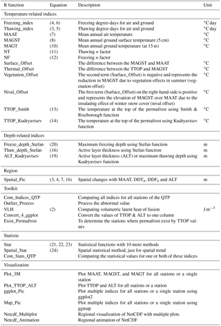
PIC v1.3 was developed in the R language and environment for statistical computing v3.3.3 and is distributed as open source software under the GNU-GPL 3.0 License (R Core Team, 2017). Therefore, the PIC v1.3 code can be modified as required to meet the needs of every user. The R package PIC v1.3 provides all the necessary functionality to perform the calculation, statistics, and drawing of permafrost indices with over 38 functions based on the user's specific requirements (see Fig. 2). The following packages are required to set up PIC v1.3 (type library(PIC)): ggplot2 (Wickham et al., 2009), ggmap (Kahle and Wickham, 2013), RNetCDF (Michna and Woods, 2013), and animation (Xie, 2013). These packages are automatically added to the R user's library during installation. A dataset that contains the daily weather observations, parameters, and information (i.e., from 1951 to 2010) of 52 weather stations in the QTP was bundled into this package. However, the regional data with the NetCDF format were placed in the GitHub repository. The dataset variables excluded in the calculation can also be used as a reference or provide support to further develop PIC. These variables include wind speed, precipitation, evaporation, humidity, and soil temperature at different depths. PIC v1.3 was primarily designed to compute indices of permafrost and seasonal frozen soil from observations and forcing data. Therefore, the current stable version of the program (v1.1) includes functionalities that cover temperature-related indices (i.e., MAAT, MAGST, and TTOP) and depth-related indices (i.e., ALT and freeze depth) that are commonly used in permafrost research. It is possible to better evaluate the changes in frozen soil by combining multiple indices for overall analysis.
2.2 Permafrost modeling
PIC v1.3 enables the calculation of the thawing–freezing degree-days for air and ground surface (DDTa∕DDTs∕DDFa∕DDFs), MAAT, MAGST, MAGT, the seasonal thawing–freezing n factor (nt∕nf), TTOP, ALT, and the maximum seasonal freeze depth (FD). The permafrost and seasonal frozen-soil indices employing the following functions are illustrated. Table 1 describes most of them.
Table 1Most important user functions in the R package PIC v1.3. The equation column of this table corresponds to the equation in Sect. 2.
As is the annual temperature amplitude at the ground surface, where Tmax and Tmin are the annual maximal and minimal temperatures, respectively. As can be calculated as follows:
L is the volumetric latent heat of fusion, ρ is the dry density of soil, and W is the water content of the soil in percentages.
DDTa and DDTs are the sums of mean daily air and ground surface above temperatures of 0 ∘C (Celsius degree-days), respectively. DDFa and DDFs are the sums of mean daily air and ground surface temperatures below 0 ∘C (Celsius degree-days), respectively. Degree-days are usually used to describe the air and ground surface temperature intensity, where Ta and Ts are the air and ground temperatures, respectively, and n is the number of days in a year (Juliussen and Humlum, 2007).
P is assigned a value of 365 days as a default value. Local variations in vegetation, topography, and snow cover may result in several differences between MAGST and MAAT. MAAT and MAGST can be computed as follows.
MAGT is defined as the soil temperature at the depth of zero annual temperature change. Tz,t is the ground temperature at any time t and depth z below a ground surface. MAGT is often found at depths from 10 to 15 m over the QTP (Wu and Zhang, 2010). Here, we take the z value of 15 m as the default value, but the user can change the depth z. MAGT can be computed (Juliussen and Humlum, 2007; Riseborough et al., 2008) as follows.
The seasonal thawing–freezing n factor (nt∕nf) relates thawing and freezing degree-days (DDTa∕DDTs∕DDFa∕DDFs) in seasonal air temperature to ground surface temperatures; nt and nf can be computed (Riseborough et al., 2008) as follows.
TTOP indicates average temperatures at the top of the permafrost. The active layer is defined as the layer of ground subject to annual thawing and freezing underlain by permafrost. ALT refers to the maximum thawing depth of the active layer. Two methods serve the same purpose when computing TTOP and ALT. The subscripts S and K stand for the Smith and Kudryavtsev functions (Kudryavtsev et al., 1977; Smith and Riseborough, 1996), respectively.
The maximum thawing depth or ALT uses the Stefan and Kudryavtsev functions (Kudryavtsev et al., 1977; Riseborough et al., 2008), where L is the latent heat of fusion for ice (3.34 × 10⁵ J kg−1).
Freeze_depths is the maximum seasonal freezing depth that uses the Stefan function, which can be computed as follows:
2.3 Statistical methods
Statistical analysis can facilitate evaluation of the trends and the overall modeling performance. In particular, each statistic has strengths and weaknesses. Thus, we adopted over 10 statistical methods to evaluate these indices in station computing for time series data. The quantitative statistics include the slope, y intercept, Pearson's correlation coefficient (R), coefficient of determination (R2), root mean square error (RMSE), standard deviation (SD), ratio of scatter (RS), normalized RMSE (NRMSE), Nash–Sutcliffe efficiency (NSE), RMSE observation standard deviation ratio (RSR), percent bias (PBIAS), normalized average error (NAE), variance ratio (VR), and index of agreement (D; Jafarov et al., 2012; Legates and McCabe, 1999). The sequential Mann–Kendall (MK) trend test was used to statistically assess whether there was a shift in trends of the climate factors and permafrost indices (Sneyers, 1990). The original MK trend test can be calculated as follows.
Two sequential series ui values can be calculated as follows:
The two series for the MK trend test, a progressive and a backward, were set up. If they cross each other and diverge beyond a specific threshold value and exceed the confidence level of 95 %, then there is a statistically significant trend shift point.
The spatial trend can also be calculated to evaluate regional computing for temporal–spatial data through the function below. The index represents one permafrost index, n represents the sequential years, and indexi is the index value in year i. Taking ALT as an example, a positive trend means that ALT was increasing, thereby indicating that permafrost degradation has intensified; a negative value means that ALT was decreasing, thereby indicating that permafrost degradation has a certain inhibition. A zero trend suggests a lack of change (Chen et al., 2014; Stow et al., 2003).
3.1 Daily weather observations
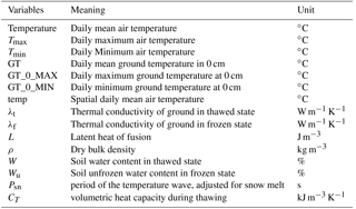
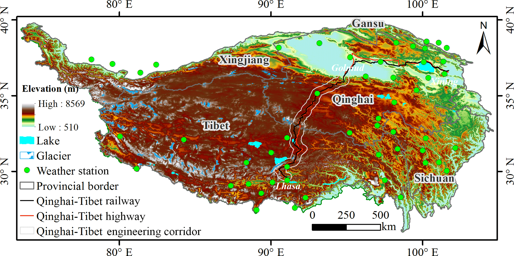
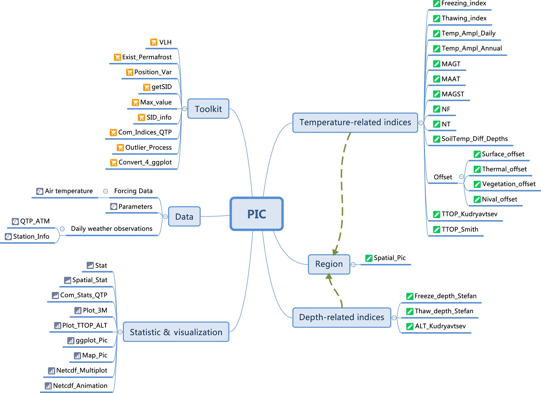
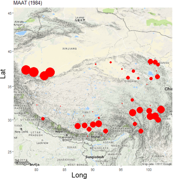
Table 2 shows detailed information of the data and parameters. Meteorological data were obtained from the China Meteorological Administration (CMA; http://www.cma.gov.cn/, last access: 18 June 2018), particularly from permanent meteorological stations across the QTP (Fig. 1). A total of 52 weather stations with daily meteorological records (i.e., from 1951 to 2010) were selected, including the daily mean, maximum (max), and minimum (min) air temperatures, wind speed, observed and corrected precipitation, evaporation, air humidity, atmospheric pressure, sunshine duration, daily mean, max, and min ground surface temperatures, and soil temperature at different depths (i.e., 5, 10, 15, 20, 40, 50, 80, 160, and 320 cm). These data have been corrected under specifications for surface meteorological observation and CMA quality control. Daily weather observations are used as the input data for the PIC v1.3 station calculation.
3.2 Atmospheric forcing dataset
Table 3Parameters of thermal conductivity in the thawed/frozen state. The UADS Code came from soil texture classification of United States Department of Agriculture (USDA). The Qinghai-Tibet Plateau does not have the 1 and 8 of soil classification codes. θ: soil water content; Kt: K value in thawed state; Kf: K value in frozen state; Cs: specific heat capacity in thawed stat (kJ kg−1 K−1).

The Qinghai–Tibet Engineering Corridor (QTEC), located at the center of the QTP, was selected in preparing the atmospheric forcing data. The Global Land Data Assimilation System (GLDAS; https://ldas.gsfc.nasa.gov, last access: 18 June 2018) and the weather station data of the surrounding QTEC were merged through spatial interpolation and offset correction to produce a new dataset for 1980 to 2010 with a daily 0.1∘ temporal–spatial resolution (Luo et al., 2018). An atmospheric forcing dataset was used as the input data for the PIC v1.3 regional calculation.
3.3 Parameters
The parameters for the ground conditions were based on soil property data and field observations. The parameter data have two sets: one for weather stations and another for the QTEC region. The Harmonized World Soil Database (HWSD, version 1.21) provides information on soil parameters that are available for evaluating soil thermal conductivity with field observations and can be used as input parameters to the PIC v1.3 package (Bicheron et al., 2008; FAO/IIASA/ISRIC/ISSCAS/JRC, 2009). The thermal conductivity of ground in a thawed or frozen state, λt and λf, can be computed through the joint parameterization scheme of the Johansen method (Johansen, 1977) and Luo parameterization (Luo et al., 2009).
The soil thermal conductivity of dry soil λdry depends on dry bulk density ρ, the thermal conductivity of soil solids λs varies with the gravel content q, λq is the thermal conductivity of quartz (7.7 W m−1 K−1), λo is the thermal conductivity of other minerals (2.0 W m−1 K−1), and q is the gravel content in the soil. The saturated soil thermal conductivity λsat depends on the thermal conductivity of soil solids λs, liquid water λw (0.594 W m−1 K−1), and the soil saturated water content θs. The degree of saturation Sr is a function of the soil water content, θ, and soil saturated water content, θs. The Kersten numbers in the thawed or frozen state, Ket and Kef, are two functions of the degree of saturation Sr and K values in the thawed or frozen state, Kt and Kf; ρ, q, and θs come from the T_BULK_DENSITY, T_GRAVEL, and T_BS fields of the HWSD.
The volumetric heat capacity during thawing, CT, is given as
where Cw is the specific heat of liquid water (4.18 kJ kg−3 K−1), and Cs is the soil specific heat capacity. θ, Cs, Kt, and Kf in different soil textures can be found in Table 3; these four parameters are empirical parameters used to explain different soil texture types based on soil texture, thermal conductivities, and specific heat capacity derived from soil sampling along the QTEC. Figure 3 shows these input spatial parameters over the QTP.
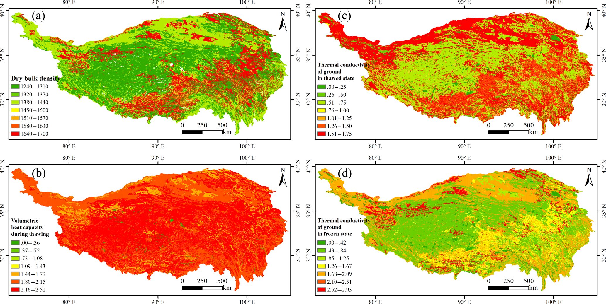
Figure 3Spatial parameters for PIC v1.3 over the Qinghai–Tibet Plateau. (a) Dry bulk density ρ; (b) volumetric heat capacity during thawing CT; (c) thermal conductivity of ground in thawed state λt; (d) thermal conductivity of ground in frozen state λf.
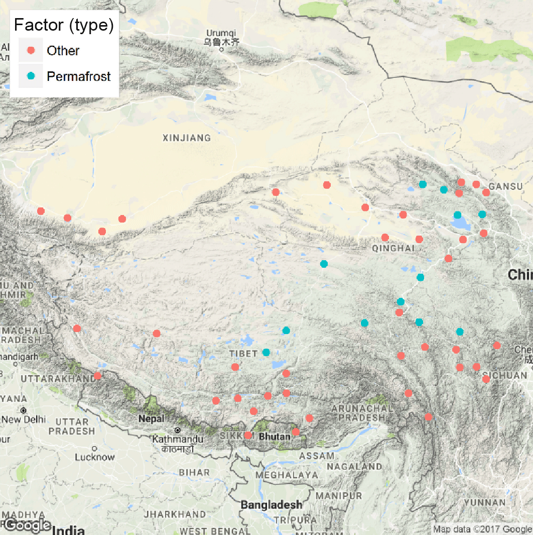
Figure 4Permafrost occurrence map. Google Maps is a base map that uses the Exist_Permaforst function. “Other” indicates seasonal frozen soil.


PIC v1.3 supports two computational modes: the station and regional calculations that enable statistical analysis and visual displays of the time series and spatial simulations. The regional calculation adopts GIS approaches to compute each spatial grid. PIC v1.3 was initially developed to address the immediate need for a reliable and easy-to-use program for estimating temporal–spatial changes in frozen QTP soil. Thus, the workflow is comprised of deliberately simplified steps throughout the entire process. Once PIC v1.3 is installed, the workflow of the weather observations is considerably straightforward: (1) an index of a weather station for one year or multiple years is calculated, (2) an index of 52 weather stations from 1951 to 2010 is calculated, and (3) an index of all stations or permafrost stations from 1951 to 2010 is drawn through a curve and spatial visualization. Step (1) is an optional step. The forcing data workflow has only two steps: (1) a total of four indices from 1980 to 2010 are calculated, including MAAT, DDTa, DDFa, and ALT, and (2) the spatial statistics and visualization of these four indices are drawn.
Several examples of PIC v1.3 use and application are presented here. This section highlights several significant features of the package in terms of specific functions, including station and regional calculation, statistics, and visualization. However, PIC v1.3 includes numerous illustrations from the literature and possible detailed analyses. PIC v1.3 has built-in station data. The dataset comprises two tables (data frame), namely QTP_ATM for daily weather observations and Station_Info for information and parameters from each station. Users can modify or adjust the parameters in the Station_Info and use the data and parameters. Additional examples can be referenced in the GitHub repository (https://github.com/iffylaw/PIC/blob/master/Examples.R, last access: 18 June 2018).
4.1 Station calculation
We can use different functions in the R console to perform the calculations based on the selected method. For example, if users want to obtain a MAAT value for a certain station year, they can enter the following command. TempName and data are optional in the MAAT function.
MAAT (Year = 1980, TempName = "Temperature",
data = QTP_ATM, SID = 52908)
A user can also obtain the MAAT values for a specified period of years in a station.
MAAT (Year = 1980:2010, TempName =
"Temperature", data = QTP_ATM, SID = 52908)
The “Year” option can be assigned to a number and sequence. The other temperature- and depth-related indices can also use the two inputs for the “Year” option. A user can obtain the values of all stations for an index. The “VarName” option can be equal to the function name in the Com_Indices_QTP function. The results can also be saved to a CSV file with column and row names. The case of the input VarName is supported.
Com_Indices_QTP (VarName = "MAAT")
Given that the freezing–thawing index can be divided into freezing–thawing degree-days of the air and ground surface, the VarName option should add “_air” or “_ground” at the ends of the Freezing_index and Thawing_index. However, the abbreviation can also be utilized as the option input. The “Thawing_index_air” and “ta” are the same.
Com_Indices_QTP (VarName =
 "Thawing_index_air")
Com_Indices_QTP (VarName = "ta")
After the TTOP indices are computed, the stations that may have permafrost should be determined. The Exist_Permafrost function can determine and map the stations where permafrost exists. The probability of permafrost occurrence and most likely permafrost conditions are determined from the computing results of the Exist_Permafrost function (see Fig. 4).
TTOP_S_QTP < - Com_Indices_QTP
 (VarName = "TTOP_Smith")
TTOP_K_QTP < - Com_Indices_QTP
 (VarName = "TTOP_Kudryavtsev")
Exist_Permafrost (plot = "yes")
The QTP measurements have consistently been difficult. The dataset has several null and anomalous values, leading to a few anomalous values in computing the indices. Accordingly, these outlier values should be processed. The Outlier_Process function seeks the outlier values and sets them to null thereafter, which is an option because abnormal values have been processed in the Com_Indices_QTP.
Outlier_Process (MAAT_QTP[,1:stations])
4.2 Regional calculation
A total of four indices, including MAAT, DDFa, DDTa, and ALT, can be computed with the atmospheric forcing dataset in PIC v1.3. This package supports NetCDF format data; thus, it reads and writes a NetCDF file to support regional computing. The input NetCDF files require a few forcing and parameter data. After the calculations, a user can compute the spatial statistics and draw the index changes through a GIF animation (see Sect. 4.3 and 4.4).
Spatial_Pic (NetCDFName = "PIC_indices.nc",
 StartYear = 1980, EndYear = 2010)
4.3 Statistics
The stat function contains all the statistical methods for station calculation. PIC v1.3 provides two calculations for computing the statistical values of all stations using Com_Stats_QTP: (1) the indices that vary with changing years and (2) the comparison of the same two indices for different computational methods. Options ind1 and ind2 were used; however, ind2 can be disregarded when computing the statistical values between a single datum and years.
Com_Stats_QTP (ind1 = MAAT_QTP)
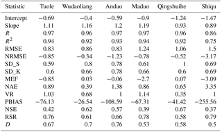
TTOP and ALT were calculated utilizing two different functions, so these two indices should be compared. For example, the two TTOP values for all QTP stations are compared. A user can assign ind1 and ind2 to compute the ALT statistical values between the Stefan and Kudryavtsev functions. Thereafter, the statistical values are saved to the CSV file when executing the Com_Stats_QTP function. Table 4 shows all the statistical values of the selected stations.
Com_Stats_QTP (ind1 = TTOP_S_QTP,
 ind2 = TTOP_K_QTP)
Com_Stats_QTP (ind1 = ALT_S_QTP,
 ind2 = ALT_K_QTP)
Table 4The statistical values of TTOP apply Com_ Stats_QTP for the stations where permafrost exists. Intercept: y-intercept; Slope: slope of regression line; R: Pearson's correlation coefficient, R2: coefficient of determination; RMSE: root mean squared error; NRMSE: normalized RMSE; SD_S: the standard deviation of TTOP using the Stefan function; SD_K: the standard deviation of TTOP using the Kudryavtsev function; MEF: modelling efficiency; NAE: normalized average error; VR: variance ratio; PBIAS: percent bias; NSE: Nash-Sutchliffe efficiency; RSR: RMSE-observations standard deviation ratio; and D: index of agreement.
A spatial trend can also be computed using the Spatial_Stat function after the regional calculation. The function simultaneously saves the spatial trend of the five indices into the NetCDF file. In addition, the function draws the animation of the spatial trend (see Sect. 4.4).
Spatial_Stat ("PIC_indices.nc", "ALT")
4.4 Visualization
Station visualization can be produced by Plot_ TTOP_ALT and Plot_3M. The Plot_TTOP_ALT function plots two TTOP or two ALT indices in a figure for all stations or stations with permafrost. VarName has the “TTOP” and “ALT” options, whereas SID has the “permafrost” and “all” options. The Plot_3M function draws the MAAT, MAGST, and MAGT indices. The two functions plot only the stations where permafrost exists when SID = “permafrost.”
Plot_TTOP_ALT (VarName = "TTOP",
 SID = "permafrost")
Plot_TTOP_ALT (VarName = "ALT",
 SID = "permafrost")
Plot_3M(SID = "permafrost")
The other approach of “ggplot2” was adopted to visualize the region (see Fig. 5).
ggplot_Pic (Type = "TTOP", SID = "permafrost")
The indices that change over time can also be plotted through a GIF animation that uses Map_Pic (Fig. 6).
Map_Pic (VarName = "TTOP_S")
Map_Pic (VarName = "TTOP_K")
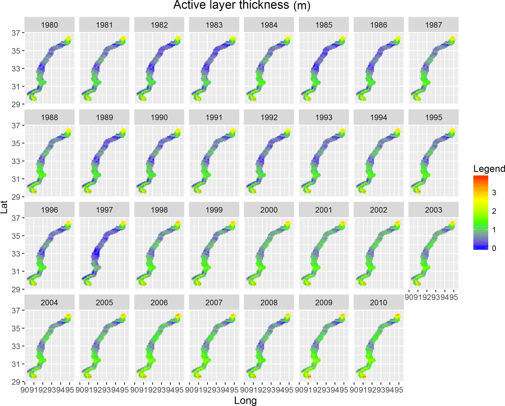
The input and output of the regional calculation can be drawn using the Netcdf_Multiplot function (see Fig. 7), which uses animation to display the values. The spatial trend can also be drawn in the Spatial_Stat apart from calculating the spatial statistics. This function draws all four indices when “VarName” has no input (see Fig. 8).
Netcdf_Multiplot (NetCDFName =
 "PIC_indices.nc", VarName = "ALT")
Netcdf_Animation (NetCDFName =
 "PIC_indices.nc", VarName = "ALT")
Spatial_Stat ("PIC_indices.nc")
5.1 PIC performance
This study proposes permafrost modeling to compute the changes in the active layer and permafrost with the climate, and this considers station and regional modeling over the QTP. We apply the two approaches to 52 weather stations and a central region of the QTP. The PIC v1.3 simulation results using the Exist_Permafrost function show that permafrost was detected at 12 of the 52 observation stations (Fig. 4). The permafrost areas began to shrink from the southern and northern parts to the central QTEC region (Fig. 7). The permafrost, whether in permafrost stations or QTEC, continued to thaw with increasing ALT, low surface offset, and thermal offset, as well as high MAAT, MAGST, MAGT, and TTOP for most areas of QTP.
PIC v1.3 computes and maps the temporal dynamics and spatial distribution of permafrost in the stations and region. There were more challenges in the regional modeling than the stations' input data and parameters. The station calculation can estimate the long-term temporal trend of permafrost dynamics, whereas the regional calculation can estimate the temporal–spatial trend. In addition, the simulated TTOP and ALT using the Stefan and Smith functions are higher than the Kudryavtsev function. Although the overall trend of TTOP and ALT are coincidental, the two different computational methods can be combined to simulate their variation. Furthermore, 16 indices can be collectively employed for a comprehensive analysis. The station and regional modeling can be integrated to evaluate the temporal–spatial evolution of permafrost in the QTP. In particular, the station modeling can be applied to validate the simulated results of the region. Moreover, the regional calculation can extend from QTEC to the entire QTP and even the other permafrost regions.
The “for” loop is discarded, whereas the “apply” functions are used extensively to significantly lower the computation time. PIC v1.3 was run natively as a single process in the Windows 7 Operating System. The calculations were performed independently through RStudio Desktop v1.1 software (RStudio, Inc., USA). The utilized processor is an Intel Core i7-2600 CPU 3.40 GHz, and the available memory is 32 GB. The current regional calculation takes only approximately 11 s. Apart from the Kudryavtsev model that requires considerable computation time (i.e., approximately 5 min), the station calculation also exhibited an improved efficiency. Therefore, PIC v1.3 can be considered an efficient R package.
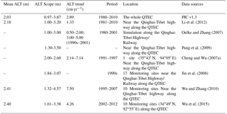
Climate change indicates a pronounced warming and permafrost degradation in the QTP with active layer deepening (Chen et al., 2013; Cheng and Wu, 2007; Wu and Zhang, 2010; Wu et al., 2010), and both the simulation of stations and the region in PIC v1.3 also show widespread permafrost degradation (Figs. 4–8). Meanwhile, as shown in Figs. 7 and 8, the permafrost in the QTEC also continued to thaw, with the ALT growing. The QTEC is the most accessible area of the QTP. Most boreholes were drilled in the QTEC to monitor changes in permafrost conditions, and these monitoring data provide support for model performance evaluation. Meanwhile, ALT was widely used, so we adopted the permafrost index to estimate PIC v1.3 simulation performance. The simulated PIC v1.3 ALT and previous literature in the QTEC are compared in Table 5. The increasing rate of ALT averaged 0.50–7.50 cm yr−1. The rate during the 1990s to 2010s was greater, at more than 4.00 cm yr−1, than during 1980 to the 1990s, at approximately 2.00 cm yr−1. Though both the observed and the simulated ALT values and their variation in different locations of the QTEC were still relatively large, the ALT trend in PIC v1.3 was close to the observations and simulation in the QTEC. In recent decades, the permafrost thaw rate has increased significantly. The majority of observed ALT and its trend along the QTH and QTR was greater than the simulated grid ALT of PIC v1.3, mainly because the observation sites are near these engineering facilities. These comparative analyses suggest that the temporal–spatial trends of permafrost conditions in the QTEC using PIC v1.3 were consistent with previous studies. More importantly, the difference between simulation results highlights the importance of the transparency and reusability of models, data, parameters, simulation results, and so on.
Table 5The active layer thickness (ALT) and its trend between the PIC v1.3 simulation and literature analysis in the Qinghai-Tibet Engineering Corridor (QTEC).
5.2 Advantages
Previous studies on the QTP (1) used one or two indices, such as MAAT and MAGST, to evaluate the permafrost changes (Yang et al., 2010), (2) constructed a regression analysis method through the relationship between MAGT and elevation, latitude, and slope aspects that presented a static permafrost distribution (Lu et al., 2013; Nan, 2005), and (3) did not share the model data and codes; hence, other researchers could not validate their results and conduct further research (McNutt, 2014). Compared with the previous permafrost modeling on the QTP, PIC v1.3 is considerably open, easy, intuitive, and reproducible for integrating data and most of the temperature- and depth-related indices. The PIC v1.3 function supports the computation of multiple indices and different time periods, and the encoding mode is reusable and universal. This package can also be easily adopted to intuitively display the changes in the active layer and permafrost, as well as assess the impact of climate change. The PIC v1.3 workflow is extremely simple and requires only one or two steps to obtain the simulated results and visual images. All running examples, data, and code can be obtained from the GitHub repository. However, the permafrost modeling integrates a gridded meteorological dataset, soil database, weather and field observations, parameters, and multiple functions and models supporting dynamic parameter changes such as vegetation and ground condition changes. Over 50 QTP weather stations were introduced, and they can partially resolve the spatial change in the permafrost area. The QTEC region is an example of spatial modeling that classifies land cover and topographic features to determine the spatial input parameters. Spatial modeling also uses the temporal–spatial data to provide spatially detailed information on the active layer and permafrost. The static–dynamic maps and statistical values of these indices can facilitate the understanding of the current condition of the near-surface permafrost and identify stations and ranges at high risk of permafrost thawing with the changing climate and human activities. Permafrost thawing causes significant changes in the environment and characteristics of frozen-soil engineering (Larsen et al., 2008; Niu et al., 2016). A comprehensive assessment of permafrost can provide guidance regarding the future of highways and high-speed railway systems in the QTP.
5.3 Limitations and uncertainties
PIC v1.3 was developed with numerous indices as well as support stations and regional simulations. PIC v1.3 can be used to estimate the frozen-soil status and possible changes over the QTP by calculating permafrost indices. This package has many engineering applications and can be used to assess the impact of climate change on permafrost. Moreover, it provides observational data and a comprehensive analysis ability for multiple indices. The probability of permafrost occurrence and the most likely permafrost conditions are determined by computing the 16 indices. Although PIC v1.3 quantitatively integrates most of them based on previous studies (Jafarov et al., 2012; Nelson et al., 1997; Riseborough et al., 2008; Smith and Riseborough, 2010; Wu et al., 2010; Zhang et al., 2005, 2014), it still has several limitations and uncertainties. First, the regional calculation is one-dimensional and assumes that each grid cell is uniform without water–heat exchange. Second, the heterogeneity in the ground conditions of the QTP also brings along uncertainties of parameter preparation. Third, soil moisture at different depths affects the thermal conductivity and thermal capacity of the soil (Shanley and Chalmers, 1999; Yi et al., 2007). Thus, the soil input parameters should be dynamically changed. Lastly, climate forcing has several uncertainties (Zhang et al., 2014), including input air and ground temperatures (i.e., the quality of the ground temperature in the QTP is currently unreliable). Thus, the regional calculation supports fewer indices than the station calculation. These deficiencies can be significant for the permafrost dynamics with environmental evolution.
An R package PIC v1.3 that computes the temperature- and depth-related permafrost indices with daily weather observations and atmospheric forcing has been developed. This package is open source software and can be easily used with input data and parameters that users can customize. A total of 16 permafrost indices for stations and the region are developed, and datasets of 52 weather stations and a central region of the QTP were prepared. Permafrost modeling and data are integrated into the PIC v1.3 R package to simulate the temporal–spatial trends of permafrost with the climate estimate and estimate the status of the active layer and permafrost in the QTP. The current functionalities also include time series statistics, spatial statistics, and visualization. Multiple visual methods display the temporal and spatial variability of the stations and the region. The package produces high-quality graphics that illustrate the status of frozen soil and may be used for subsequent publication in scientific journals and reports. The simulated PIC v1.3 results generally indicate that the temporal–spatial trends of permafrost conditions essentially agree with previously published studies. The transparency and repeatability of the PIC v1.3 package and its data can be used to assess the impact of climate change on permafrost. Additional features may be implemented in future releases of PIC to broaden its application range. In the future, the observational data of the active layer will be integrated into the PIC datasets, and the simulation results will be compared with it. PIC v1.3 will also be used to predict the future state of permafrost by utilizing projected climate forcing and scenarios. Additional functions and models will be absorbed into PIC to improve the simulation and perform comparative analyses with other functions and models. Parallel computation will be added to improve the computation efficiency. The key impact that PIC v1.3 is expected to provide to the open community is an increase in consistency within and comparability among studies. Furthermore, we encourage contributions from other scientists and developers, including suggestions and assistance, to modify and improve the proposed PIC v1.3.
The PIC v1.3 code that supports the findings of this study is stored in the GitHub repository (https://github.com/iffylaw/PIC; Luo, 2018).
The data are included in the Supplement files and/or the GitHub repository.
The supplement related to this article is available online at: https://doi.org/10.5194/gmd-11-2475-2018-supplement.
The authors declare that they have no conflict of interest.
This research was supported by the National Natural Science Foundation of
China (41301508, 41630636, 41771074). We would like to express our gratitude
to the editor and the two anonymous reviewers for their insightful comments
and suggestions that improved this paper.
Edited
by: David Lawrence
Reviewed by: two anonymous referees
Bicheron, P., Defourny, P., Brockmann, C., Schouten, L., Vancutsem, C., Huc, M., Bontemps, S., Leroy, M., Achard, F., and Herold, M.: GLOBCOVER: products description and validation report, Foro Mundial De La Salud, 17, 285–287, 2008.
Chen, B. X., Zhang, X. Z., Tao, J., Wu, J. S., Wang, J. S., Shi, P. L., Zhang, Y. J., and Yu, C. Q.: The impact of climate change and anthropogenic activities on alpine grassland over the Qinghai-Tibet Plateau, Agr. Forest Meteorol., 189, 11–18, 2014.
Chen, H., Zhu, Q. A., Peng, C. H., Wu, N., Wang, Y. F., Fang, X. Q., Gao, Y. H., Zhu, D., Yang, G., Tian, J. Q., Kang, X. M., Piao, S. L., Ouyang, H., Xiang, W. H., Luo, Z. B., Jiang, H., Song, X. Z., Zhang, Y., Yu, G. R., Zhao, X. Q., Gong, P., Yao, T. D., and Wu, J. H.: The impacts of climate change and human activities on biogeochemical cycles on the Qinghai-Tibetan Plateau, Glob. Change Biol., 19, 2940–2955, 2013.
Chen, S., Liu, W., Qin, X. Y., Liu, Y., Zhang, T., Chen, K., Hu, F., Ren, J., and Qin, D.: Response characteristics of vegetation and soil environment to permafrost degradation in the upstream regions of the Shule River Basin, Environ. Res. Lett., 7, 045406, https://doi.org/10.1016/j.agrformet.2014.01.002, 2012.
Cheng, G. and Wu, T.: Responses of permafrost to climate change and their environmental significance, Qinghai-Tibet Plateau, J. Geophys. Res.-Earth, 112, https://doi.org/10.1111/gcb.12277, 2007a.
Sneyers, R.: On the statistical analysis of series of observations, World Meteorological Organization, Geneva, Switzerland, Technical note No. 143, p. 192, 1990.
Gisnås, K., Etzelmüller, B., Farbrot, H., Schuler, T. V., and Westermann, S.: CryoGRID 1.0: Permafrost Distribution in Norway estimated by a Spatial Numerical Model, Permafrost Periglac., 24, 2–19, 2013.
Harris, C., Arenson, L. U., Christiansen, H. H., Etzemuller, B., Frauenfelder, R., Gruber, S., Haeberli, W., Hauck, C., Holzle, M., Humlum, O., Isaksen, K., Kaab, A., Kern-Lutschg, M. A., Lehning, M., Matsuoka, N., Murton, J. B., Nozli, J., Phillips, M., Ross, N., Seppala, M., Springman, S. M., and Muhll, D. V.: Permafrost and climate in Europe: Monitoring and modelling thermal, geomorphological and geotechnical responses, Earth-Sci. Rev., 92, 117–171, 2009.
Hilbich, C., Hauck, C., Hoelzle, M., Scherler, M., Schudel, L., Voelksch, I., Muehll, D. V., and Maeusbacher, R.: Monitoring mountain permafrost evolution using electrical resistivity tomography: A 7-year study of seasonal, annual, and long-term variations at Schilthorn, Swiss Alps, J. Geophys. Res.-Earth, 113, F01S90 https://doi.org/10.1029/2007JF000799, 2008.
Jafarov, E. E., Marchenko, S. S., and Romanovsky, V. E.: Numerical modeling of permafrost dynamics in Alaska using a high spatial resolution dataset, The Cryosphere, 6, 613–624, https://doi.org/10.5194/tc-6-613-2012, 2012.
Jin, H., Yu, Q., Wang, S., and Lü, L.: Changes in permafrost environments along the Qinghai–Tibet engineering corridor induced by anthropogenic activities and climate warming, Cold Reg. Sci. Technol., 53, 317–333, https://doi.org/10.1016/j.coldregions.2007.07.005, 2008.
Johansen, O.: Thermal Conductivity of Soils, 1977, University of Trondheim, Norway, 1977.
Juliussen, H. and Humlum, O.: Towards a TTOP ground temperature model for mountainous terrain in central-eastern Norway, Permafrost Periglac., 18, 161–184, 2007.
Kahle, D. and Wickham, H.: ggmap: Spatial Visualization with ggplot2, R. J., 5, 144–161, 2013.
Kudryavtsev, V. A., Garagulya, L. S., Yeva, K. A. K., and Melamed, V. G.: Fundamentals of Frost Forecasting in Geological Engineering Investigations, Hanover, New Hampshire, Cold Regions Research and Engineering Lab, 489, 1977.
Larsen, P. H., Goldsmith, S., Smith, O., Wilson, M. L., Strzepek, K., Chinowsky, P., and Saylor, B.: Estimating future costs for Alaska public infrastructure at risk from climate change, Global Environ. Chang., 18, 442–457, 2008.
Legates, D. R. and McCabe, G. J.: Evaluating the use of “goodness-of-fit” measures in hydrologic and hydroclimatic model validation, Water Resour. Res., 35, 233–241, 1999.
Lewkowicz, A. G. and Bonnaventure, P. R.: Interchangeability of mountain permafrost probability models, northwest Canada, Permafrost Periglac., 19, 49–62, 2008.
Li, L., Yang, S., Wang, Z. Y., Zhu, X. D., and Tang, H. Y.: Evidence of Warming and Wetting Climate over the Qinghai-Tibet Plateau, Arct. Antarct. Alp. Res., 42, 449–457, 2010.
Li, R., Zhao, L., Ding, Y., Wu, T., Xiao, Y., Du, E., Liu, G., and Qiao, Y.: Temporal and spatial variations of the active layer along the Qinghai-Tibet Highway in a permafrost region, Chinese Sci. Bull., 57, 4609–4616, https://doi.org/10.1657/1938-4246-42.4.449, 2012.
Lu, J., Niu, F., Cheng, H., Lin, Z., Liu, H., and Luo, J.: The Permafrost Distribution Model and Its Change Trend of Qinghai-Tibet Engineering Corridor, J. Mt. Sci.-Engl., 31, 226–233, 2013.
Luo, L.: PIC: Comprehensive R package for permafrost indices computing, Zenodo, https://doi.org/10.5281/zenodo.1254848, 2018.
Luo, L., Zhang, Y., and Zhu, W.: E-Science application of wireless sensor networks in eco-hydrological monitoring in the Heihe River basin, China, Iet Sci. Meas. Technol., 6, 1–8, https://doi.org/10.1049/iet-smt.2011.0211, 2012.
Luo, L., Ma, W., Zhang, Z., Zhuang, Y., Zhang, Y., Yang, J., Cao, X., Liang, S., and Mu, Y.: Freeze/Thaw-Induced Deformation Monitoring and Assessment of the Slope in Permafrost Based on Terrestrial Laser Scanner and GNSS, Remote Sens., 9, 198, https://doi.org/10.3390/rs9030198, 2017.
Luo, L., Ma, W., Zhuang, Y., Zhang, Y., Yi, S., Xu, J., Long, Y., Ma, D., and Zhang, Z.: The impacts of climate change and human activities on alpine vegetation and permafrost in the Qinghai-Tibet Engineering Corridor, Ecol. Indic., 93, 24–35, 2018.
Luo, S., Lü, S., and Zhang, Y.: Development and validation of the frozen soil parameterization scheme in Common Land Model, Cold Reg. Sci. Technol., 55, 130–140, 2009.
McNutt, M.: Journals unite for reproducibility, Science, 346, 679–679, 2014.
Michna, P. and Woods, M.: RNetCDF – A Package for Reading and Writing NetCDF Datasets, R. J., 5, 29–36, 2013.
FAO/IIASA/ISRIC/ISSCAS/JRC: Harmonized World Soil Database (version 1.2), FAO, Rome, Italy and IIASA, Laxenburg, Austria, available at: http://webarchive.iiasa.ac.at/Research/LUC/External-World-soil-database/HTML/, last access: 18 June 2018.
Nan, Z.: Prediction of permafrost distribution on the Qinghai-Tibet Plateau in the next 50 and 100 years, Sci. China Ser. D, 48, 797–804 https://doi.org/10.1360/03yd0258, 2005.
Nelson, F. E., Shiklomanov, N. I., Mueller, G. R., Hinkel, K. M., Walker, D. A., and Bockheim, J. G.: Estimating active-layer thickness over a large region: Kuparuk River Basin, Alaska, USA, Arct. Antarct. Alp. Res., 29, 367–378, 1997.
Niu, F., Luo, J., Lin, Z., Fang, J., and Liu, M.: Thaw-induced slope failures and stability analyses in permafrost regions of the Qinghai-Tibet Plateau, China, Landslides, 13, 55–65, 2016.
Oelke, C. and Zhang, T.: Modeling the Active-Layer Depth over the Tibetan Plateau, Arct. Antarct. Alp. Res., 39, 714–722, 2007.
Pang, Q., Cheng, G., Li, S., and Zhang, W.: Active layer thickness calculation over the Qinghai–Tibet Plateau, Cold. Reg. Sci. Technol., 57, 23–28, 2009.
Ran, Y., Li, X., and Cheng, G.: Climate warming over the past half century has led to thermal degradation of permafrost on the Qinghai–Tibet Plateau, The Cryosphere, 12, 595–608, https://doi.org/10.5194/tc-12-595-2018, 2018.
Ran, Y. H., Li, X., Cheng, G. D., Zhang, T. J., Wu, Q. B., Jin, H. J., and Jin, R.: Distribution of Permafrost in China: An Overview of Existing Permafrost Maps, Permafrost Periglac., 23, 322–333, 2012.
R Core Team: R: A language and environment for statistical computing, R Foundation for Statistical Computing, Vienna, Austria, 2017.
Riseborough, D.: Permafrost Modeling, in: Encyclopedia of Snow, Ice and Glaciers, edited by: Singh, V. P., Singh, P., and Haritashya, U. K., Springer Netherlands, Dordrecht, 2011.
Riseborough, D., Shiklomanov, N., Etzelmuller, B., Gruber, S., and Marchenko, S.: Recent advances in permafrost modelling, Permafrost Periglac., 19, 137–156, 2008.
Romanovsky, V. E. and Osterkamp, T. E.: Thawing of the active layer on the coastal plain of the Alaskan Arctic, Permafrost Periglac., 8, 1–22, 1997.
Sazonova, T. S. and Romanovsky, V. E.: A model for regional-scale estimation of temporal and spatial variability of active layer thickness and mean annual ground temperatures, Permafrost Periglac., 14, 125–139, 2003.
Shanley, J. B. and Chalmers, A.: The effect of frozen soil on snowmelt runoff at Sleepers River, Vermont, Hydrol. Process., 13, 1843–1857, 1999.
Shen, M. G., Piao, S. L., Jeong, S. J., Zhou, L. M., Zeng, Z. Z., Ciais, P., Chen, D. L., Huang, M. T., Jin, C. S., Li, L. Z. X., Li, Y., Myneni, R. B., Yang, K., Zhang, G. X., Zhang, Y. J., and Yao, T. D.: Evaporative cooling over the Tibetan Plateau induced by vegetation growth, P. Natl. Acad. Sci. USA, 112, 9299–9304, 2015.
Smith, M. W. and Riseborough, D. W.: Permafrost monitoring and detection of climate change, Permafrost Periglac., 7, 301–309, 1996.
Smith, S. L. and Riseborough, D. W.: Modelling the thermal response of permafrost terrain to right-of-way disturbance and climate warming, Cold. Reg. Sci. Technol., 60, 92–103, 2010.
Stow, D., Daeschner, S., Hope, A., Douglas, D., Petersen, A., Myneni, R., Zhou, L., and Oechel, W.: Variability of the seasonally integrated normalized difference vegetation index across the north slope of Alaska in the 1990s, Int. J. Remote Sens., 24, 1111–1117, 2003.
Wickham, H., Lawrence, M., Cook, D., Buja, A., Hofmann, H., and Swayne, D. F.: The plumbing of interactive graphics, Computation Stat., 24, 207–215, 2009.
Wu, Q., Hou, Y., Yun, H., and Liu, Y.: Changes in active-layer thickness and near-surface permafrost between 2002 and 2012 in alpine ecosystems, Qinghai–Xizang (Tibet) Plateau, China, Global Planet. Change, 124, 149–155, 2015.
Wu, Q. B. and Zhang, T. J.: Changes in active layer thickness over the Qinghai-Tibetan Plateau from 1995 to 2007, J. Geophys. Res.-Atmos., 115, D09107, https://doi.org/10.1029/2009jd012974, 2010.
Wu, Q. B., Zhang, T. J., and Liu, Y. Z.: Permafrost temperatures and thickness on the Qinghai-Tibet Plateau, Global Planet. Change, 72, 32–38, 2010.
Xie, Y. H.: animation: An R Package for Creating Animations and Demonstrating Statistical Methods, J. Stat. Softw., 53, 1–27, 2013.
Yang, M. X., Nelson, F. E., Shiklomanov, N. I., Guo, D. L., and Wan, G. N.: Permafrost degradation and its environmental effects on the Tibetan Plateau: A review of recent research, Earth-Sci. Rev., 103, 31–44, 2010.
Yao, T., Pu, J., Lu, A., Wang, Y., and Yu, W.: Recent glacial retreat and its impact on hydrological processes on the tibetan plateau, China, and sorrounding regions, Arct. Antarct. Alp. Res., 39, 642–650, 2007.
Yi, S., Wang, X., Qin, Y., Xiang, B., and Ding, Y.: Responses of alpine grassland on Qinghai-Tibetan plateau to climate warming and permafrost degradation: a modeling perspective, Environ. Res. Lett., 9, 074014, https://doi.org/10.1088/1748-9326/9/7/074014, 2014a.
Yi, S., Wischnewski, K., Langer, M., Muster, S., and Boike, J.: Freeze/thaw processes in complex permafrost landscapes of northern Siberia simulated using the TEM ecosystem model: impact of thermokarst ponds and lakes, Geosci. Model Dev., 7, 1671–1689, https://doi.org/10.5194/gmd-7-1671-2014, 2014b.
Yi, S., Woo, M. K., and Arain, M. A.: Impacts of peat and vegetation on permafrost degradation under climate warming, Geophys. Res. Lett., 34, L16504, https://doi.org/10.1029/2007GL030550, 2007.
Zhang, T., Barry, R. G., Knowles, K., Heginbottom, J. A., and Brown, J.: Statistics and characteristics of permafrost and ground-ice distribution in the Northern Hemisphere, Polar Geography, 31, 132–154, 2008.
Zhang, T., Frauenfeld, O. W., Serreze, M. C., Etringer, A., Oelke, C., McCreight, J., Barry, R. G., Gilichinsky, D., Yang, D., Ye, H., Ling, F., and Chudinova, S.: Spatial and temporal variability in active layer thickness over the Russian Arctic drainage basin, J. Geophys. Res.-Atmos., 110, D16101, https://doi.org/10.1029/2004JD005642, 2005.
Zhang, Y., Carey, S. K., and Quinton, W. L.: Evaluation of the algorithms and parameterizations for ground thawing and freezing simulation in permafrost regions, J. Geophys. Res.-Atmos., 113, D17116, https://doi.org/10.1029/2007JD009343, 2008.
Zhang, Y., Olthof, I., Fraser, R., and Wolfe, S. A.: A new approach to mapping permafrost and change incorporating uncertainties in ground conditions and climate projections, The Cryosphere, 8, 2177–2194, https://doi.org/10.5194/tc-8-2177-2014, 2014.