the Creative Commons Attribution 4.0 License.
the Creative Commons Attribution 4.0 License.
 | 06 Jul 2018
GEM-MACH-PAH (rev2488): a new high-resolution chemical transport model for North American polycyclic aromatic hydrocarbons and benzene
Cynthia H. Whaley
Elisabeth Galarneau
Paul A. Makar
Ayodeji Akingunola
Wanmin Gong
Sylvie Gravel
Michael D. Moran
Craig Stroud
Junhua Zhang
Qiong Zheng
Environment and Climate Change Canada's online air quality forecasting model, GEM-MACH, was extended to simulate atmospheric concentrations of benzene and seven polycyclic aromatic hydrocarbons (PAHs): phenanthrene, anthracene, fluoranthene, pyrene, benz(a)anthracene, chrysene, and benzo(a)pyrene. In the expanded model, benzene and PAHs are emitted from major point, area, and mobile sources, with emissions based on recent emission factors. Modelled PAHs undergo gas–particle partitioning (whereas benzene is only in the gas phase), atmospheric transport, oxidation, cloud processing, and dry and wet deposition. To represent PAH gas–particle partitioning, the Dachs–Eisenreich scheme was used, and we have improved gas–particle partitioning parameters based on an empirical analysis to get significantly better gas–particle partitioning results than the previous North American PAH model, AURAMS-PAH. Added process parametrizations include the particle phase benzo(a)pyrene reaction with ozone via the Kwamena scheme and gas-phase scavenging of PAHs by snow via vapour sorption to the snow surface.
The resulting GEM-MACH-PAH model was used to generate the first online model simulations of PAH emissions, transport, chemical transformation, and deposition for a high-resolution domain (2.5 km grid cell spacing) in North America, centred on the PAH data-rich region of southern Ontario, Canada and the northeastern US. Model output for two seasons was compared to measurements from three monitoring networks spanning Canada and the US Average spring–summertime model results were found to be statistically unbiased from measurements of benzene and all seven PAHs. The same was true for the fall–winter seasonal mean, except for benzo(a)pyrene, which had a statistically significant positive bias. We present evidence that the benzo(a)pyrene results may be ameliorated via further improvements to particulate matter and oxidant processes and transport. Our analysis focused on four key components to the prediction of atmospheric PAH levels: spatial variability, sensitivity to mobile emissions, gas–particle partitioning, and wet deposition. Spatial variability of PAHs ∕ PM2.5 at a 2.5 km resolution was found to be comparable to measurements. Predicted ambient surface concentrations of benzene and the PAHs were found to be critically dependent on mobile emission factors, indicating the mobile emissions sector has a significant influence on ambient PAH levels in the study region. PAH wet deposition was overestimated due to additive precipitation biases in the model and the measurements. Our overall performance evaluation suggests that GEM-MACH-PAH can provide seasonal estimates for benzene and PAHs and is suitable for emissions scenario simulations.
- Article
(5542 KB) -
Supplement
(1437 KB) - BibTeX
- EndNote


Polycyclic aromatic hydrocarbons (PAHs) are semi-volatile atmospheric pollutants that have numerous negative health effects (some are carcinogenic, mutagenic, and teratogenic) (Kim et al., 2013). Measurements of PAHs in North America are sparse in both time (typically 24 h averages, every 6 days) and space (limited surface measurement networks), yet show ambient concentrations that regularly exceed the Ontario provincial government's health-based threshold (Galarneau et al., 2016). Similarly, benzene is a gas-phase single-ring aromatic hydrocarbon, is a known carcinogen, and also exceeds atmospheric health-based guidelines (Galarneau et al., 2016). Accurate, 3-D modelling of PAHs and benzene can fill in the space–time gaps of the measurements, identify atmospheric processes that are responsible for the threshold exceedances, and simulate effects of emissions scenarios.
AURAMS (A Unified Regional Air-quality Modelling System) was an offline (meteorology from a weather forecast model used as an input), Eulerian 3-D chemical transport model (CTM) developed by Environment and Climate Change Canada (ECCC). In Galarneau et al. (2014), AURAMS was modified to include seven PAH species (phenanthrene, anthracene, fluoranthene, pyrene, benz(a)anthracene, chrysene, and benzo(a)pyrene – hereafter abbreviated to PHEN, ANTH, FLRT, PYR BaA, CHRY, and BaP, respectively). AURAMS-PAH included emissions, transport, gas–particle partitioning, oxidation of the gas-phase PAHs with OH, dry deposition, and wet deposition of the particle-phase PAHs. This model was able to accurately simulate the 2002 annual average PAH concentrations in North America when compared to 45 measurement sites, located in Ontario, the northeastern US, and California. However, the AURAMS-PAH gas–particle partitioning over-predicted the gas phase for the lighter PAH species, and was employed at relatively poor time and spatial resolutions. It was also missing two known PAH loss processes: the surface reaction of O3 on particulate BaP (Kwamena et al., 2004, 2007; Ringuet et al., 2012; Keyte et al., 2013; Liu et al., 2014), and snow scavenging of gas-phase PAHs (Franz and Eisenreich, 1998; Daly and Wania, 2004; Lei and Wania, 2004; Skrdlíková et al., 2011). These missing processes, along with the coarse (42 km) spatial resolution, may have contributed to the differences between model results and measurements. Also, this model used PAH emission factors for mobile emissions which are now out of date for representing the modern vehicle fleet.
Other PAH CTMs include the following: GEOS-Chem (Friedman and Selin, 2012; Thackray et al., 2015), which is a global model; CMAQ, which was run on the Europe continental domain in Aulinger et al. (2007) and in North America in Zhang et al. (2016, 2017); and FARM (Flexible Air quality Regional Model) (Gariazzo et al., 2007), which is a regional model, applied for the Rome region in Italy. The most relevant of these model studies to our own is that by Zhang et al. (2016, 2017), whereby they ran CMAQ with 16 PAH species added, at 36 km resolution in a mainly US domain (that included parts of Canada and Mexico), evaluated their model results against NATTS measurements, and used their results to determine the cancer risk to the US human populations from various sources.
Therefore, the goal of this study is to update and improve ECCC's PAH modelling capabilities by using a more advanced model framework, updating emission inventories, and utilizing better process representation of PAHs than were used in AURAMS-PAH to allow better exploration of PAH processes and scenarios. To achieve this goal, GEM-MACH (Global Environmental Multiscale model – Modelling Air quality and CHemistry), ECCC's next generation, online air quality forecasting model (meteorology and air quality are predicted in the same code) was modified to include the same seven PAH species, as well as benzene. The paramaterization of PAH processes was improved in the following ways: (1) on-road mobile PAH emissions were updated with more recent data, to better represent the modern vehicle fleet; (2) gas–particle partitioning parameters were improved based on empirical results and analysis of AURAMS model output; (3) process representation for the on-particle O3 – particulate BaP reaction was added to the model; and (4) process representation for in- and below-cloud wet scavenging (including scavenging by snow) were added for gas-phase PAHs and benzene. Simulations using GEM-MACH-PAH were then carried out at high (2.5 km) spatial resolution in a small, but densely populated North American domain including southern Ontario, and most of the northeastern US (Fig. 1) for summer and winter of 2009. We refer to this region as the “Pan Am” domain because it was created for high-resolution air quality modelling during the 2015 Pan American Games in Ontario (Joe et al., 2017). This domain contains approximately 109 million people, including about 38 % of the Canadian population and 30 % of the US population. The model results were evaluated using measurements from a high spatial resolution campaign in Hamilton, Ontario (Anastasopoulos et al., 2012), as well as the binational Integrated Atmospheric Deposition Network (IADN), the Canadian National Air Pollution Surveillance network (NAPS), and the US National Air Toxics Trends Stations network (NATTS). We focus our model evaluation on spatial variations at high resolution, estimating the level of model sensitivity to uncertainties in the PAH emission factors, gas–particle partitioning, and wet deposition, which are all related to novel aspects of the GEM-MACH-PAH model.
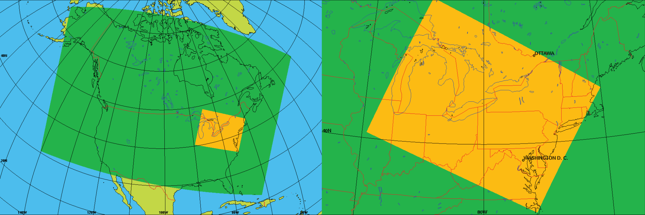
Figure 1North American model domain with 10 km horizontal grid spacing (green), and the nested “Pan Am” model domain with 2.5 km horizontal grid spacing (orange).
The following sections will further describe the GEM-MACH-PAH model (Sect. 2), the measurements used for evaluation (Sect. 3), the results of the model evaluation (Sect. 4), and the conclusions (Sect. 5).
In the present study, we have modified ECCC's high-resolution air quality forecasting model, GEM-MACH (hereafter called “GEM-MACH-PAH”), to include benzene and seven PAHs (in both gas and particle-phases) and have carried out 6 months of simulations in 2009 at the highest resolution (2.5 km grid cell size) in a North American domain yet reported for PAH simulations (to our knowledge). We have also tracked PAH wet deposition, and gas–particle partitioning, and have attempted to qualify model sensitivity to uncertainty in mobile emission factors, which has not been reported in other model studies.
2.1 GEM-MACH overview
GEM-MACH is an online, 3-D chemical transport model, which is embedded in GEM, ECCC's operational numerical weather prediction model (Côté et al., 1998b, a; Moran et al., 2010) (available online here: https://github.com/mfvalin?tab=repositories, last access: 3 July 2018). Online models such as GEM-MACH improve air-quality chemical prediction performance by reducing interpolation errors between different model coordinate systems and removing the input/output time and disk storage required for the transfer of meteorological input files to their offline CTM counterparts (e.g., Baklanov et al., 2014). The coupling to meteorology is a one-way process in this version, whereby chemistry does not influence the meteorology. More detailed description of the gas-, aqueous-, and particle-phase process representations of GEM-MACH, and an evaluation of its performance for common pollutants such as ozone, particulate matter (PM), and ammonia appears in Moran et al. (2013), Makar et al. (2015a, b), Gong et al. (2015), and Whaley et al. (2018b). Here we will focus on the model changes made to include PAH species and processes.
GEM-MACH is used to provide ECCC's twice daily, 48 h operational public forecasts of criteria air pollutants (ozone, nitrogen oxides, and PM), as well as the Air Quality Health Index (https://ec.gc.ca/cas-aqhi/, last access: 3 July 2018.). To reduce the computational burden for forecasting, the PM size distribution is represented using a simplified sectional treatment consisting of two size bins, a fine-fraction bin for particles with Stokes diameter from 0 to 2.5 µm and a coarse-fraction bin for particles with Stokes diameter from 2.5 to 10 µm (Moran et al., 2010), with sub-binning used for those particle processes requiring a finer particulate size distribution. Here, we utilize the research version of GEM-MACH version 2, revision 2476, with this two-size-bin representation as our starting point for PAH modifications. The model grid used corresponds to a rotated latitude–longitude map projection with 2.5 km horizontal grid spacing and a hybrid vertical coordinate with 80-level vertical discretization spanning the atmosphere from the surface to 0.1 hPa.
2.2 Model modifications for benzene and PAH species
Our modifications to GEM-MACH include adding benzene and 7 gas-phase and 14 particle-phase (7 species × 2 size bins) PAHs to the species arrays. The gas–particle partitioning subroutine described in Galarneau et al. (2014) was also added, but with updated partitioning parameters (see Sect. 2.2.1). Since PAHs have very small concentrations relative to criteria air contaminants, as in Galarneau et al. (2014), we assume they do not have a significant effect on oxidant concentrations (O3 and OH). Thus, the PAHs in GEM-MACH-PAH make use of the outcomes of the model's gas- and aqueous-phase chemistry in a diagnostic fashion for PAH oxidation. Processes in which the PAHs directly participate include advection, vertical diffusion, plume rise of major point source emissions, aerosol particle microphysics, in- and below-cloud scavenging, and dry and wet deposition of both gas and particle phases. Some of these processes and/or their controlling parameters were updated relative to Galarneau et al. (2014) and are described in the subsections below. Like AURAMS-PAH, the total (gas+particle) PAH emissions were treated as gas-phase emissions in GEM-MACH-PAH, since these quickly repartition between particles and gas phases following emission. The non-PAH and PAH emissions are described further below. The MACH part of the model code is available online (Whaley et al., 2018a; https://doi.org/10.5281/zenodo.116225), and the call sequence of the code is included in Sect. S5 of the Supplement.
2.2.1 Gas–particle partitioning
As PAHs are semi-volatile organic compounds that partition between the particulate and gaseous phases of the atmosphere, their partitioning is a major determinant of their atmospheric fate (Bidleman, 1988). Despite decades of study (Junge, 1977; Yamasaki et al., 1982; Bidleman and Foreman, 1987; Pankow, 1987; Smith and Harrison, 1996; Dachs and Eisenreich, 2000; Lohmann and Lammel, 2004; Keyte et al., 2013), the mechanisms responsible for PAH partitioning and its spatiotemporal variability are not well-understood. AURAMS-PAH included two parametrizations to calculate gas–particle partitioning: Junge–Pankow, JP (Junge, 1977; Pankow, 1987) and Dachs–Eisenreich, DE (Dachs and Eisenreich, 2000), both of which, when applied for partitioning in AURAMS-PAH, assigned too much PAH mass to the gas phase. The two schemes resulted in surprisingly similar gas–particle partitioning (Galarneau et al., 2014). We carried out post-processing and analysis on the AURAMS-PAH model output from both schemes as well as the observations of gas and particle PAHs from the Galarneau et al. (2014) study, in order to determine which scheme to proceed with in GEM-MACH-PAH, and how it could be improved.
Measured PAH partitioning typically takes the linear form of
where Kp,k is the partitioning coefficient for each PAH species, k:
and Cp, CTSP, and Cg are the concentrations of the particulate PAH, the total suspended particles, and the gas-phase PAH, respectively. is the sub-cooled liquid vapour pressure of the kth gas, and mk and bk are empirically derived coefficients. This linear relationship (where the logKp of all PAH species in any given measurement sample fall on a line relative to their logpL) is common among homologous compound groups such as PAHs, polychlorinated biphenyls (PCBs), and polychlorinated dioxins and furans. However, the JP formulation only allows for (see Sect. S2 in the Supplement for more detailed information and a derivation). Conversely, observation-based estimates show a wide variety of values that are usually less than 1 (e.g., Fig. S2a in the Supplement), and this could be the reason why the AURAMS-PAH JP model results under-predicted the particulate fraction.
Therefore, we proceeded with the Dachs–Eisenreich formulation in GEM-MACH, but with improved parameters. The Dachs–Eisenreich (DE) partitioning formulation was adapted from work examining water–sediment partitioning (Dachs and Eisenreich, 2000). The DE expression for Kp (Eq. S2.2.1) is related to the octanol–air and soot–air (KSA,k) partitioning coefficients, the latter depending on the soot–water (KSW,k) and air–water partitioning coefficients. The soot–water partitioning coefficients are highly uncertain. Their values in the literature span two orders of magnitude for the same compound (Dachs and Eisenreich, 2000; Bucheli and Gustafsson, 2000; Jonker and Koelmans, 2002; Xu et al., 2012). KSW,k from Jonker and Koelmans (2002), was used in AURAMS-PAH. However, using the 2002 measurement data and their average mK, we have determined new KSW,k values based on ambient observations that improve the DE particulate fraction representation (see Sect. S2.3 in the Supplement for this process, and Table 1 for the original and new values). The purple boxes in Fig. 2 represent the results of the AURAMS-PAH partitioning module, making use of our new KSW,k values instead of the originals.

Figure 2All-site ensemble of modelled/measured ratios of logKp (a) and particulate fraction (b) for each PAH. Shown are the “adjusted model” (purple, from Eq. S2.2.4) and the original AURAMS-PAH model (green). Box and whiskers: thick line is the median, boxes extend to the 25th and 75th percentiles, and whiskers extend to the minimum and maximum.
Table 1Original (from Galarneau et al., 2014, based on Jonker and Koelmans, 2002) and adjusted (based on AURAMS-PAH model–measurement analysis for North America) KSW values, along with other KSW cited in the literature. All values are × 105, and unitless.
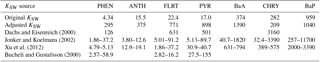
While the adjusted KSW values in Table 1 are significantly different from those in the original model (based on Jonker and Koelmans, 2002 as adjusted by the relative contributions of PM mass to the domain total in the inventory of Galarneau et al., 2007), particularly for lower molecular-weight species, they fall within the range of values found in the literature (e.g., Dachs and Eisenreich, 2000; Bucheli and Gustafsson, 2000; Jonker and Koelmans, 2002; Xu et al., 2012). The large correction and large range of published KSW,k values (which lack a temperature dependence) lends further support for the need to measure KSA,k directly on soots of atmospheric relevance so that they need not be estimated based on the highly uncertain/variable KSW,k.
2.2.2 Emissions
Chemical (non-PAH) emissions in GEM-MACH make use of data from the US Environmental Protection Agency (EPA)'s 2011 National Emissions Inventory (NEI), and Canada's 2010 Air Pollutant Emission Inventory (APEI), these being the closest available inventory years to the year in which our simulations take place (2009). PAH model emissions were created with the SMOKE emissions processing system (Sparse Matrix Operator Kernel Emissions, https://www.cmascenter.org/smoke/, last access: 3 July 2018), which utilized PAH-to-TOG (total organic gases) emission factors (originally compiled for AURAMS-PAH by Galarneau et al. (2007, 2014)). Below we outline the further modifications and updates that we made to this existing emissions database, in order to generate updated PAH emissions for modelling.
PAH stationary emissions. Most of the PAH emission factors (EFs) used for the 2002 AURAMS-PAH model were compiled from the US EPA's Locating and Estimating Series (US EPA, 1998), the AP-42 document (US EPA, 1995), and the 1999 National Emissions Inventory (NEI99), (Galarneau et al., 2007). PAH EFs for stationary sources that were published between 1999 and the present are not substantially different from those already being used in SMOKE. For example, recent literature on agricultural burning (e.g., Dhammapala et al., 2007; Hall et al., 2012) reported EFs that were close (within a factor of two) to those already in the inventory. Only emissions from iron and steel production were updated to those in Odabasi et al. (2009) for electric arc furnaces, as the values used in Galarneau et al. (2007) were derived from literature published before 1990, and were 1–2 orders of magnitude larger (hence likely represented outdated (or absent) pollution control equipment).
PAH mobile emissions. On-road mobile PAH emission factors in AURAMS-PAH were taken from NEI99 (Galarneau et al., 2007). The mobile emissions in this inventory may no longer be relevant as the values compiled were from an older (1990s) vehicle fleet. Therefore, we employed updated EFs for more current on-road mobile emissions in Canada and the US for 2009 modelling. Also, some off-road emissions, such as emissions from helicopters and marine sources (large ships) were not previously considered and were added to the inventory (from Chen et al., 2006 and Agrawal et al., 2008, respectively) in this study.
MOVES 2014, the latest version of the US EPA's motor vehicle emissions simulator (https://www.epa.gov/moves, last access: 3 July 2018) contains a more recent standard set of mobile EFs; these are separated into one set of factors for gasoline vehicles, based on one large study of vehicles in the US (Kishan et al., 2008), and one set of factors for diesel vehicles, based on another large study in the US (Khalek et al., 2009). In order to investigate whether these US values would be representative of conditions in Canada and whether only having these two fuel-type categories is adequate, when this would neglect studies that have reported different EFs for several different vehicle/fuel categories (e.g., cars, trucks, buses, motorcycles; light- or heavy-duty; gasoline or diesel), we compiled and researched PAH-to-TOG emission factors for these classes of mobile sources from over 30 recent (1999 to present) publications, as well as from the US EPA's SPECIATE v4.4 database (containing data from 1990 to 2012: https://www.epa.gov/air-emissions-modeling/speciate-version-45-through-40, last access: 3 July 2018). Please refer to Section C in the supplemental material for this mobile emission factor analysis. In this analysis, we found that the MOVES2014 EFs provided the best results in the model and they were selected for use in our simulations.
2.2.3 On-particle BaP-O3 reaction
The only PAH oxidation reactions included in AURAMS-PAH were temperature-independent OH reactions with each gas-phase PAH species (Galarneau et al., 2014), which were also added to the GEM-MACH-PAH model. Temperature-dependent OH reaction rates were not pursued because Brubaker and Hites (1998) determined that only kOH for fluoranthene has a slight temperature dependence, but the dependence was smaller than their error levels. Also, Friedman and Selin (2012) performed a phenanthrene sensitivity study with their model, and determined that including temperature dependence in kOH did not affect their mean non-urban mid-latitude concentrations.
The AURAMS-PAH model overestimated BaP concentrations compared to measurements (Galarneau et al., 2014). This could be due to two O3-related factors: (1) particulate BaP measurements are known to be affected by on-filter O3 degradation, causing measured particulate BaP measurements to be biased low (Menichini, 2009); (2) heterogeneous BaP degradation by O3 in ambient air (Keyte et al., 2013) was not simulated in AURAMS-PAH, thereby biasing modelled concentrations high. Therefore, we added a particle-phase BaP–O3 reaction in GEM-MACH-PAH to account for the latter atmospheric process as described next. For the former, on-filter O3 reaction, we have attempted to correct the measurements as described in Sect. 3.
In GEM-MACH-PAH we used the Kwamena scheme (Kwamena et al., 2004) for the atmospheric on-particle BaP-O3 reaction, as this scheme produced the best results in Friedman and Selin (2012)'s global model, and according to our sensitivity calculations, other schemes either overestimate (e.g., Pöschl et al., 2001) or underestimate (e.g., Kahan et al., 2006) the amount of BaP destroyed by this reaction. The Kwamena scheme was used because it produced BaP loss consistent with measurement studies (Ringuet et al., 2012; Jariyasopit et al., 2014; Liu et al., 2014). The reaction rate, k, is expressed as follows:
where, .018 −1 and cm3. The Kwamena scheme is expressed in the model as
where δt is the model time step in seconds. This formulation does not depend on the particle size, but rather on the overall bulk particulate concentration, and the concentration of O3.
2.2.4 Dry and wet removal of PAHs and benzene
Gas-phase dry deposition follows a multiple resistance approach and single-layer “big leaf” approach (Wesely, 1989; Zhang et al., 2002; Makar et al., 2018) with a temperature dependency for Henry's law constants and for water solubility (Sander, 1999; Ma et al., 2010). Dry deposition of benzene and PAHs is also output by the model; however, measurements of the deposition flux of these species were unavailable during the study period.
PAH particle-phase dry deposition is treated following Zhang et al. (2001), resulting in size-dependent particle deposition velocities.
Gas-phase benzene and PAHs undergo cloud and rain scavenging via Henry's law. Henry's law partition coefficients (KAW) for the seven PAHs are proportional to inverse temperature. The mass of benzene and PAHs in the gas-phase (as opposed to the aqueous phase in cloud droplets and raindrops) is derived from
and solving for mgas:
where, is the initial mass of the gas-phase PAH before the Henry's law partitioning, and the remaining PAH mass is scavenged to the liquid rain or cloud phases (maq). Once the gaseous PAHs are scavenged to cloud-water (which is recalculated at each time step), they are subject to rain-out (cloud-to-rain conversion) process. At the end of each chemistry step, the fraction of the dissolved tracers not removed by the rain-out process will be returned to gas phase. For the fraction that do go into rain water, there is a parametrization in the rain scavenging code for re-evaporation of the rain before it reaches the ground. That fraction of PAHs would also return to the atmosphere. The remaining fraction that is not re-evaporated is counted towards the wet deposition in the model, which is irreversible (i.e., no re-emission of PAHs from the ground after they are deposited).
Note that Okochi et al. (2004) reported that assuming Henry's law equilibrium for benzene under-predicts the extent of wet-deposition. In the absence of a suitable alternative parameterization, we used Henry's law partitioning and obtained a conservative estimate of wet deposition for benzene. Note that benzene wet deposition is not evaluated in this paper as no measurements are available.
Where temperatures are < 0 ∘C below-cloud, or 15 ∘C in-cloud, scavenging of gas-phase benzene and PAHs by snow and cloud-ice is done via surface adsorption following the formulation used in Franz and Eisenreich (1998), which was also used by Wania et al. (1999), Lei and Wania (2004) and Friedman and Selin (2012):
In Eq. (7), Wg is the gas scavenging ratio (equal to the concentration of PAH in snow over the concentration of PAH in air – both in moles m−3), Kia,k is the interfacial adsorption coefficient (equal to the mass adsorbed per surface area of snow to the atmospheric vapour phase concentration – both in ng m−3), SA is the specific surface area of the snow crystal, for which we use a constant 1 m2 g−1 based on literature values for fresh snow precipitation, which are highly variable, and for which no clear relationship with temperature or wind speed has been found (Hoff et al., 1998; Hanot and Dominé, 1999; Domine et al., 2007; Hachikubo et al., 2014), ρ is the density of ice (0.917 g cm−3), and Kia,k is calculated from the following (Franz and Eisenreich, 1998):
Eq. (7) is used to determine the fraction of PAH mass in the gas and snow/cloud-ice phases.
Particle-phase PAHs are treated as passive tracers that undergo wet removal along with the modelled aerosol particles (Gong et al., 2006; Wang et al., 2010). The cloud and precipitation processes above are applied sequentially in the model using operator splitting, and the amount of PAH deposited from wet deposition is output by the model. Table S4 in the Supplement provides all of the constants used in the model.
2.3 Model setup for two three-month simulations
GEM-MACH-PAH (rev2488) was run from 8 May to 13 August 2009 and from 18 October 2009 to 5 January 2010, where the first week from each period is treated as a spin-up period (for chemical concentrations to stabilize and for the initial condition effects to be negligible: e.g., Samaali et al., 2009), and were not used in our evaluation. The time periods were chosen to coincide with as many PAH concentration and deposition measurements as possible, while limiting simulation duration to reduce computational expenses.
The chemical initial and boundary conditions for the outer nest North American domain were taken from a 1-year MOZART simulation for all pollutants (Emmons et al., 2010; Pendlebury et al., 2017), except for benzene and PAHs. Initial and boundary conditions for PAHs and benzene were set to zero for the North American domain as its boundaries are generally away from PAH and benzene sources (e.g., over the ocean), and are also very distant from the Pan Am domain. The simulations for the nested Pan Am region were run using the chemical initial and boundary conditions from the 10 km North American model run.
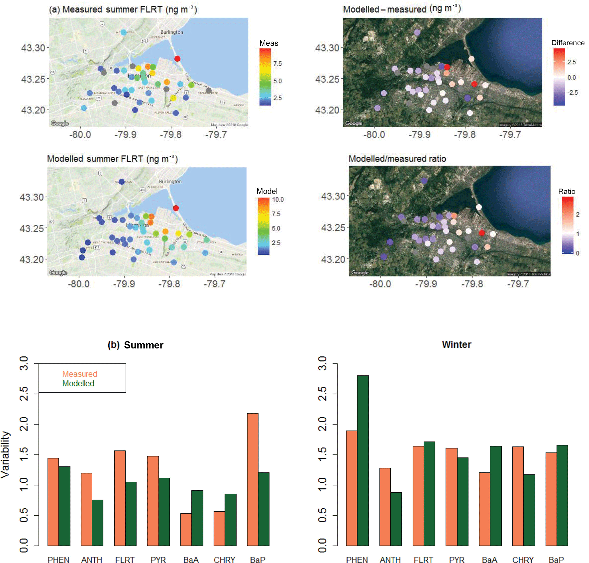
Figure 4(a) Map of 2-week summertime average fluoranthene concentrations in Hamilton, Ontario: (left) from measurements and GEM-MACH-PAH model, and (right) their differences and ratios. Note the grey dots are measurement sites that had missing data during this time period. (b) Spatial variability in the Hamilton data in (left) summer, and (right) winter.
The model simulation was carried out in sequence of 27 h staggered simulations starting at 00:00 UTC, in order to re-initialize meteorology with the analysis at 10 km resolution. The first 3 h in the 2.5 km domain were discarded as spin-up to reduce the dependency on the 10 km resolution meteorological initial conditions. Each 27 h simulation used the chemical concentrations from the end of the previous simulation as initial conditions for the next 27 h, and this sequence continued until each 3-month period was complete.
GEM-MACH-PAH was run in the two-size-bin mode to represent the PM size distribution, which means that particles fall in either fine mode (PM2.5 – diameter 2.5 µm or less) or coarse mode (PM10–PM2.5 – diameter 2.5–10 µm).
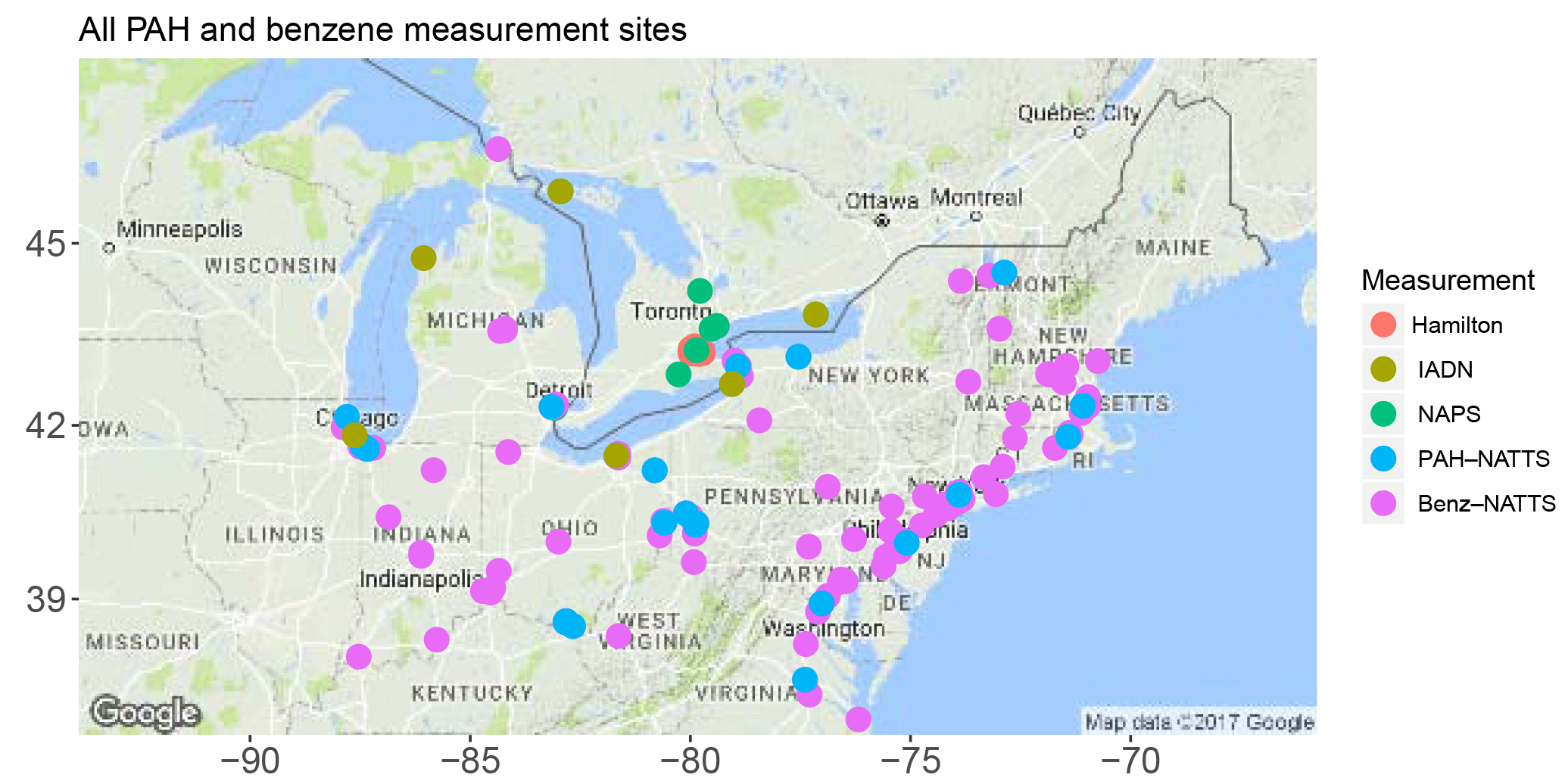
We compare the GEM-MACH-PAH predictions to all of the benzene and PAH measurements available in the Pan Am domain during the two time periods in 2009. These include a high spatial resolution urban measurement campaign in the Hamilton, Ontario region, as well as network monitoring stations from NAPS, NATTS, and IADN. Locations of PAH and benzene measurement stations are plotted in Figs. 3 and 4a. Note that all measurement stations were not equipped with oxidant removal technology; therefore, all measured PAHs, especially benzo(a)pyrene (which has the highest particulate fraction, and is the most reactive with O3), would have had losses due to reaction with ozone on the filters (Menichini, 2009; Liu et al., 2014); thus, measured PAHs would be biased low compared to concentrations in ambient air. Accordingly, we have applied an O3 correction to the BaP measurements in this study, as the literature suggests that the BaP sampling artifact is substantial, with around 20–72 % lost on average during sampling (Menichini, 2009; Liu et al., 2014). Note that our correction follows the linear method recommended by Schauer et al. (2003), which is dependent only on O3 concentrations. However, other studies state that the O3 degradation of BaP is more complex, with additional dependencies on the resident atmospheric lifetime of BaP (Goriaux et al., 2006), and relative humidity (Pitts Jr. et al., 1986; Umwelterhebungen and Gerätesichereit, 2002; Menichini, 2009). However, those studies did not provide an alternative correction equation. Therefore, in our results, we will present both the Schauer-corrected BaP measurements (for sites that had O3 monitors nearby), as well as the original reported BaP from the measurements, given the lack of a better correction for the sampling artifact.
3.1 Hamilton measurement campaign
Ambient measurements of PM2.5 and 16 PAH species were collected from a dense network of measurement sites in Hamilton, Ontario during June/July 2009 and December 2009. These measurements are described in Anastasopoulos et al. (2012), where they found a high level of intra-urban variability for the PAHs; 3–4 times more variable than PM2.5 concentrations.
There were 43 measurement sites operating during the summer period (see Fig. 4a), and 46 sites during the winter period. All measurements are from 2-week integrated time frames (24 June to 8 July and 2 to 16 December) taken with URG personal pesticide samplers, which collected gas and particle-phase PAHs less than 2.5 µm in diameter in 40 m3 of sample air. The PM2.5 measurements were made at the same sites using a three-stage Harvard cascade impactor. The particle-phase PAHs (up to 2.5 µm in diameter) were collected on a Teflon filter, gas-phase PAHs were collected in polyurethane foam (PUF), and total (gas+particle) PAHs concentrations were reported in ng m−3 as determined by gas chromatography/mass selective detection. PM sample filter masses were determined by gravimetric analysis (Anastasopoulos et al., 2012).
O3 measurements that were used to correct the Hamilton BaP measurements came from three monitoring sites in the Hamilton region (“Downtown”, “Mountain”, and “West”) from the Ontario Ministry of Environment and Climate Change (MOECC) website for historical air quality data (http://www.airqualityontario.com/history/, last access: 3 July 2018).
3.2 National Air Pollution Surveillance program
NAPS is a Canadian program to provide accurate and long-term air quality data of a uniform standard across the country. NAPS is managed under a cooperative agreement between ECCC and the provinces, territories, and some municipal governments. There are currently 286 NAPS measurement sites in 203 communities located in every province and territory (https://open.canada.ca/data/en/dataset/1b36a356-defd-4813-acea-47bc3abd859b, last access: 3 July 2018).
Under this program, PAH samples were collected over 24 h, beginning and ending at midnight (local time; LT), typically every 6 days, with a sample volume range of 600–800 m3 (Environment Canada, 2013). Benzene samples were collected in 6 L stainless steel canisters over 24 h, starting at midnight, every 3 days (Galarneau et al., 2016).
Within the Pan Am domain, total PAHs (gas+particle-phases combined) and benzene were measured at eight NAPS sites (listed in Table S1 in the Supplement; Fig. 3), and their 2009 data were downloaded from the following url: http://maps-cartes.ec.gc.ca/rnspa-naps/data.aspx (last access: 3 July 2018).
For BaP measurement corrections, the NAPS network also measures hourly O3 at four of these eight PAH/benzene sites (Windsor, Hamilton, Simcoe, and Egbert). Two of the missing sites (Toronto and Etobicoke) had nearby O3 measurements from MOECC, but the last two (Burnt Island, and Point Petre), which are rural sites, had no O3 measurements nearby. Therefore, BaP could only be corrected at six of the eight NAPS sites in the Pan Am domain.
3.3 National Air Toxics Trends Stations network
NATTS is a US program to monitor toxic air pollutants in accordance with the US Government Performance Results Act, which requires the US EPA to reduce the risk of cancer and other serious health effects associated with hazardous air pollutants (HAPS) by achieving a 75 % reduction in toxic chemical emissions in air, based on 1993 levels (US EPA, 2009). Regulated under the Clean Air Act are 188 HAPS species including benzene and the 7 PAHs in this study.
Every 6 days, 24 h ambient air samples are collected starting at midnight (00:00 LT). Analysis of the samples is done by high-resolution gas chromatography/mass spectrometry (GCMS) selective ion monitoring (SIM) mode to get total (gas+particle) PAH concentrations, and benzene concentrations (Eastern Research Group, Inc., 2009).
There are 115 NATTS sites within the model domain (Table S1 in the Supplement, Fig. 3), but only 21 sites measured PAHs, while 113 sites measured benzene. Those data were downloaded from the following url: https://www3.epa.gov/ttnamti1/toxdat.html#data (last access: 3 July 2018). Measurement methods in NATTS are very similar to those of NAPS.
Since O3 was not measured at the NATTS sites, NATTS BaP was corrected with the nearest O3 monitor data found at the US EPA and CASTNET websites: https://www.epa.gov/outdoor-air-quality-data/download-daily-data (last access: 3 July 2018) and https://java.epa.gov/castnet/reportPage.do (last access: 3 July 2018), respectively.
3.4 Integrated Atmospheric Deposition Network
IADN was mandated by the 1987 Great Lakes Water Quality Agreement, and was initiated in 1990 to measure atmospheric concentrations of persistent toxic pollutants in the Great Lakes basin. There are nine IADN sites total within our Pan Am model domain, and they are listed in Table S1 of the Supplement (see also Fig. 3). Six of the nine IADN sites report gas- and particle-phase PAH atmospheric concentrations separately (labelled “PAHs” in Table S1), and a different set of six sites report wet deposition of PAHs (labelled “PAH wet dep” in Table S1) using sampled precipitation concentrations (Blanchard et al., 2005). Thus, these data can be used to evaluate the model's gas–particle partitioning and deposition, respectively. Benzene was not measured by IADN, nor was CTSP or PM10 in 2009, with the unfortunate result that Kp can not be directly calculated from the IADN measurements. O3 was also not measured by IADN, necessitating the use of the nearest O3 monitors in order to carry out the BaP oxidation correction. This latter step was only possible for observation stations at Cleveland and Chicago. The other four IADN air sites were rural/background locations, and did not have any O3 measurements nearby.
PAHs were collected by a high-volume sampler for periods of 24 h beginning at 08:00 EST, every 12 days. At Canadian IADN sites, glass fiber filters and PUF sorbent collected the particulate and gaseous fractions, whereas the US stations collected PAHs with quartz fiber filters and XAD resin (Blanchard et al., 2005). Sample volume for the US method is about 800 m3, but is 400 m3 for the Canadian method to minimize the breakthrough of volatile species during warm summer months (Blanchard et al., 2005).
Wet deposition of PAHs are measured with MIC-B precipitation collectors. The US stations used XAD-2 resin column cartridges for accumulating the organics on a 28-day cumulative basis, while the Canadian stations use a dichloromethane solvent extraction system, also on a 28-day cumulative basis. Both countries collect samples on a monthly basis. Note that one of the six wet deposition sites, St Clair, Ontario (STC), only had valid measurements during February 2009, which was not a time period simulated here. Therefore, only five IADN sites appear in our wet deposition analysis in Sect. 4.4 below.
Note that Point Petre and Burnt Island are NAPS stations co-located with IADN. IADN data were downloaded from the following url: http://donnees.ec.gc.ca/data/air/monitor/monitoring-of-combined-atmospheric-gases-and-particles/anthropogenic-organic-pollutants-in-air/ (last access: 3 July 2018).
In this section we evaluate GEM-MACH-PAH's performance for benzene and PAH surface concentrations, their spatial variation, gas–particle partitioning, and wet deposition. We also assess the sensitivity of the model output to PAH emission factors for mobile sources.
4.1 PAH concentrations in the Hamilton region
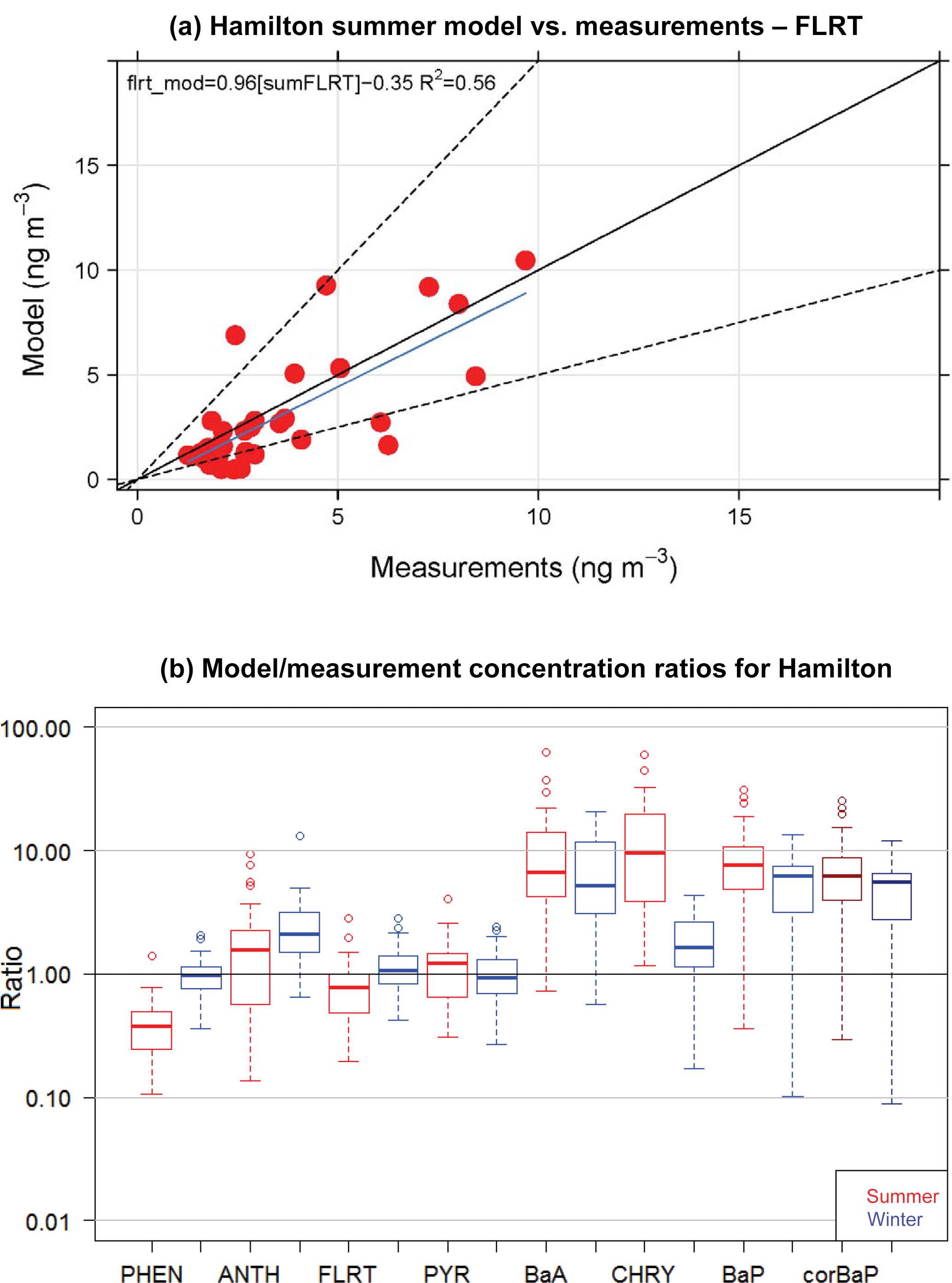
Figure 5(a) GEM-MACH-PAH model vs. measurement scatter plot of 2-week summertime fluoranthene concentrations at 40+ sites in Hamilton. (b) Frequency distributions of GEM-MACH-PAH model/measurement ratios of PAH concentrations for the Hamilton model–measurement pairs for all sites from both summer and winter. Darker-coloured boxes are results from O3-corrected BaP measurements.
GEM-MACH-PAH output for gas+fine-PM PAH were compared to measurements of same from the 2009 Hamilton campaign (Anastasopoulos et al., 2012). Figure 4a shows a map of measured and modelled fluoranthene concentrations (14-day average) in the summer time period, as well as their differences and ratios. Here we see that GEM-MACH-PAH has captured intra-city variability, and that the differences between observations and simulated values are, at a maximum, 2.8 times too high. The model is biased low in the upwind/background areas of the city, and a high in the eastern areas of the city (Fig. 4a); this pattern is seen across all seven PAHs. The spatial pattern in the PAH bias is less apparent when PAH ∕ PM2.5 ratios are plotted (in ng µg−1 – shown in Fig. S6.1 in the Supplement) – removing the dependency on modelling PM correctly (since fractions of the PAH are particulate). Therefore, the spatial pattern in the PAH bias is mainly due to the pattern in the model PM bias, which is shown in Fig. S6.2 in the Supplement.
When the spatial variability is represented by the standard deviation over the mean (σ/mean), the model achieves very similar spatial variability to the measurements (Fig. 4b). The scatter plot of model vs measurements for summertime fluoranthene concentrations (Fig. 5a, FLRT selected as a good example) has a correlation coefficient (R2) of 0.57, and the slope of the best-fit line is 0.96. The other PAH species had similar results, where, except for FLRT, the slopes and R2 values were better in the winter than in the summer.
The model bias (given as a model/measurement ratio) for all PAHs is shown as box and whiskers in Fig. 5b. Here we see that wintertime biases are smaller than those in the summertime for all PAHs except for ANTH. The four lightest PAHs (left side of Fig. 5b) have model/measurement ratios near one (except summertime PHEN), but the three heaviest PAHs, are biased high (except for wintertime CHRY). We will see this same pattern for the model bias (small for lighter PAHs, high for BaA and BaP) in the next sections as well.
BaA and BaP are the most reactive of the heavier species; thus, the lack of O3 correction to the BaA measurements may be partially responsible for the model–measurement differences. However, mean O3 for the three measurement stations in the Hamilton region was only 20–26 ppbv day−1, which meant that the O3-corrected BaP was approximately 20 % greater than the reported BaP concentrations. The median BaP bias was brought down to 6.2 from 7.6 in the summer, and 5.5 from 6.3 in the winter – these are shown as the purple boxes in Fig. 5b. Additional reactions with BaA and BaP (e.g., with NO3) are noted in the literature (Keyte et al., 2013), but were not included in GEM-MACH-PAH at this time, given larger uncertainties in those reactions. However, our model biases appear to indicate that those missing reactions may need to be considered for further model improvement. Indeed, a back-of-the-envelope calculation using a reaction rate reported in Liu et al. (2012) implied that the lifetime of particulate BaA with respect to a heterogeneous reaction with NO3 (using mean nighttime concentrations of NO3 from the model) was about 1 h. More research should be undertaken to determine the range of uncertainty for this reaction and whether it should go into PAH models. Additionally, Mu et al. (2018) suggest that the heterogeneous BaP–O3 reaction should be temperature-, humidity-, and organic aerosol phase state-dependent (none of which were taken into account in the Kwamena scheme used in our work). However, it has been shown that the Kwamena scheme and the Mu scheme produce similar results in mid-latitudes (where our study is located) (Mu et al., 2018). Spring/summertime BaP would be minimally affected, as outdoor temperatures at that time of year resemble the room temperature laboratory conditions that the Kwamena scheme was based on. Additionally, our positive model bias would likely increase in the fall–wintertime, when low temperatures and humidity would increase BaP lifetime in the Mu scheme.
In order to remove the impact of the model's PM predictions on the PAH comparison, we also plotted the PAH ∕ PM2.5 model-over-measurement ratios (shown in Fig. S6.3). There we see all of the ratios reduced – which improves results for the heavier PAHs, but increases the low bias for the lighter PAHs. The reason the bias decreases for all seven PAHs is that the model PM2.5 is overestimated by a factor of 2 in the summertime, and a factor of 1.4 in the wintertime (average across all sites in the Hamilton region).
4.2 PAH and benzene concentrations from the NAPS, NATTS, and IADN networks
Modelled 24 h-average total (gas+particle) PAH and benzene concentrations can be evaluated with measurements (taken every sixth day) from the NATTS, NAPS, and IADN surface measurement networks, which sample much of the model domain well (Fig. 3). As with the Hamilton evaluation, the model has very good agreement for seasonal averages at the monitoring network sites for benzene, phenanthrene, anthracene, fluoranthene, and pyrene, which all have model/measurement ratios (red and blue boxes) close to one, and their concentrations (green and orange boxes) overlapping in Fig. 6a. The 24 h average model (daily) and measurements (every sixth day) have been averaged over each of the 3-month time periods. BaA and CHRY are within a factor of 5 of the measurements in the summertime, but worse in the wintertime. BaP is overestimated by the model in both summer and winter by about a factor of 10, although the measurement-corrected BaP has a slightly reduced bias. We have not shown the O3-corrected BaP measurements in the plots because the changes are small, similar to the Hamilton plot (Fig. 5a).
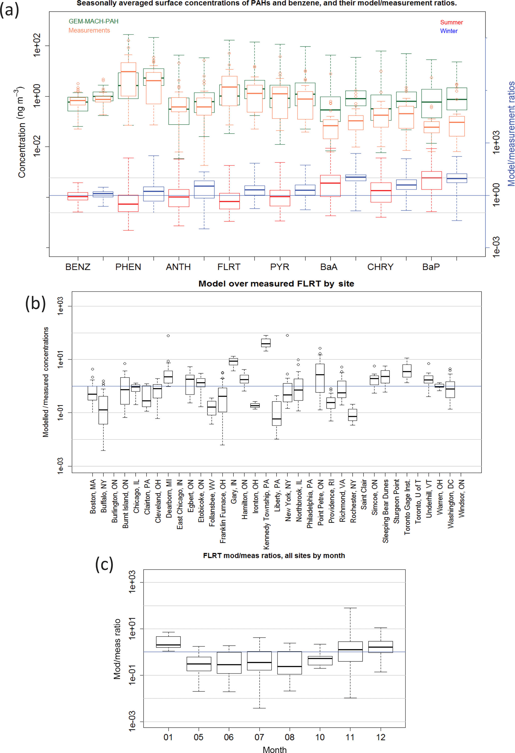
Figure 6(a) Frequency distributions of GEM-MACH-PAH (green) and measured (orange) benzene (gas) and PAH (gas+particle) seasonal average concentrations at all IADN, NAPS, and NATTS sites. Modelled/measured concentration ratios also shown for summer (red) and winter (blue), with grey lines indicating agreement within an order of magnitude. (b) Modelled/measured concentrations for each daily model–measurement pair, separated by site (FLRT given as example); (c) same as (b) but separated by month.
When the model biases are examined more closely we find a few patterns to determine the cause(s). The following list summarizes some observations from our evaluation of each model–measurement pair (24 h averages, not seasonal averages):
-
By site – overestimates: all PAHs are significantly overestimated at the Kennedy Township, Pennsylvania (northwest of Pittsburgh) NATTS site (Fig. 6b). There appears to be a major emissions point source near that station that is emitting too much PAH in our model compared to reality. There are in fact hundreds of point sources in the emissions inventory that are within 20 km of Kennedy Township, but one in particular emits a relatively large amount of VOCs, and is associated with the “Secondary Metal Production; Aluminum; Raw Material Charging” source category, which has very large PAH-to-TOG EFs in Galarneau et al. (2007) because aluminum smelter emissions are largely particulate; therefore, expressing EFs as a large fraction of TOG was somewhat artificial. However, our results indicate that the PAH EFs for that PAH speciation profile (1036b) should be reduced substantially compared to Galarneau et al. (2007). In order to ensure that this facility did not begin operation after 2009 – which is a risk when using a 2011 inventory to model the year 2009 and would result in a large overestimation – we have further verified that the facility existed and was emitting similar VOC amounts in the NEI2008 inventory as well.
PHEN (Fig. 7c) and ANTH (not shown) are also greatly overestimated in New York City, although none of the other PAHs are biased particularly high there. However, we note that the measurements for New York City appear erroneously low, as the reported PHEN concentrations there are around the same magnitude as those in Underhill, VT (Fig. 7c), which is a background site near a national park.
Most PAHs are also overestimated at the Gary, Indiana site (Fig. 6b), which may also have a nearby major point emissions source that is too high compared to reality. Furthermore. the heavier PAHs (BaA, CHRY, and BaP) are overestimated at the Toronto Gage Institute NAPS site, but are only slightly higher there than the average model/measurement ratio for those species (not shown).
-
By site – underestimates: all PAHs are markedly underestimated at the Liberty, Pennsylvania site (e.g., Figs. 6b, and 7c), implying that there may be industry emissions of PAHs here that are missing, misallocated, or misplaced in the NEI2011 inventory, or an improper PAH speciation profile applied. Similarly, PAHs are underestimated in Buffalo, New York, and at Franklin Furnace, Ohio. As these are not large cities, there may be industrial emissions that are not reported in the NEI2011 emissions inventory (or are reported at too low levels) – perhaps because those facilities shut down in 2010 (or installed emission control technology), which would mean the problem simply lies in using a 2011 inventory to model 2009.
However, when we further investigated stacks near Buffalo, NY, we found that the facility with the largest CO and VOC emissions had zero PAH emissions. This facility is associated with the generic process of “Primary metal production; By-product Coke Manufacturing”, which did not have an associated PAH-to-TOG profile in Galarneau et al. (2007), because the source category codes that follow it (such as flushing liquor circulation tank, excess-ammonia liquor tank, tar dehydrator, tar interceding sump, tar storage, and so on) are not expected to emit PAHs to air. However, our results imply that the PAH speciation profile for “By Product Coke Oven Stack Gas” (0011b) would have been more appropriate for this facility and its use might eliminate the model bias near Buffalo in future studies.
-
By month: all PAH species have lower mod/meas ratios in the summer than in the winter (shown in Fig. 6a by season for all PAHs and in Fig. 6c for FLRT by month) – implying that modelled hydroxyl radical (OH) and/or PM biases (which have strong seasonal cycles) are impacting modelled PAHs. For example, if model OH is too high in the summer, or too low in the winter, this would cause the U-shaped pattern that we see when plotting model/measurement ratio vs. month (Fig. 6c) and it would be particularly pronounced for the lighter, gas-phase PAHs, which it is. Another possibility is seasonal bias in the representation of atmospheric vertical stability: if the modelled stability is too low in the summer and too high in the winter, then winter emissions will tend to be trapped in inversions more than observed, and summer emissions will be diluted by excessive vertical mixing. However, evidence in Makar et al. (2010) and Stroud et al. (2012) suggest that model stability is too high (not too low) for the summer time period in those studies.
-
By season: for the four lightest PAHs, the model/measurement ratios are < 1 in the summer, and > 1 in the winter (Fig. 6a). As mentioned above, this is likely due to modelled OH being too high in the summer and too low in the winter. BaA and CHRY follow a similar seasonal difference but do not straddle the ratio = 1 mark.
BaP, in comparison, has a model/measurement ratio that is slightly higher in the summer than in the winter (Fig. 6a). For BaP, the OH bias could be offset by an opposite O3 bias in the model. Indeed, it has been shown (Makar et al., 2010; Stroud et al., 2012) that the processes in GEM-MACH cause urban surface O3 to be too low in the summertime, due to insufficient vertical mixing and excessive titration from NOx, and surface PM tends to be too high in the wintertime due to an overestimation of wintertime atmospheric stability (e.g., lack of an urban heat island parameterization in the driving meteorology). These factors, together with the BaP measurement bias due to on-filter reaction with O3, may explain the high model BaP bias.

Figure 7Phenanthrene time series for the summer 2009 period for the IADN (binational), NAPS (Canada), and NATTS (US) networks. Orange represents the measurements, dark green represents the base GEM-MACH-PAH model, light green represents GEM-MACH-PAH with 0.5× mobile emissions, and cyan represents GEM-MACH-PAH with 2.0× mobile emissions.
Thus, the generally high bias of modelled BaP may to be due to additive OH, O3, and PM model biases (plus the missing O3 denuder technology in the measurements), impacting BaP more than the other species because BaP has the highest O3 reactivity and the highest particulate fraction of the seven PAHs examined here.
When the five measurement sites mentioned in “By Site”, above (Kennedy Township, PA; Gary, IN; Liberty PA; Buffalo, NY; and Franklin Furnace, OH) are removed from the NATTS analysis (because errors in their nearby emissions were identified), model–measurement correlation (R) and slopes improve. For example, the model vs. measurement best-fit line slope for PHEN doubles from 0.3 to 0.6 when those sites are removed, and its R increases from 0.16 to 0.32. The slopes and R values of the four heaviest PAHs all move from negative to positive. PYR has the largest improvement, going from a slope of −0.049 and R of −0.028 to a slope of 0.26 and R of 0.35. To the extent that the model prediction errors at the other sites may reflect emissions inaccuracy, having an accurate major point emission inventory for the time period modelled, along with proper PAH speciation profiles are extremely important requirements for modelling PAHs well at high resolution. The cases with large discrepancies mentioned above highlight the need to be as specific as possible when assigning source category codes to facility processes (which is difficult given that there are tens of thousands of point sources in the inventories).
In addition to emissions errors (for which fine temporal information is lacking), transport errors can cause poorer agreement between model and measurements at high spatial- and time-scales. For example, PAH concentrations have sharp gradients and large dynamic range. Thus, if plume transport is off by a few kilometres, the result will be a very large difference between modelled and measured concentrations downwind of point sources.
That said, when doing a paired t test on all data in the model domain to examine whether the summertime and wintertime modelled averages are the same as the measured averages, we found that the model was indistinguishable from the measurements for all PAH species (t<1 and p>0.05), except for wintertime BaP (which has t>1, and p<0.05, even with the O3-corrected measurements). At finer time scales (e.g., daily model–measurement pairs) only modelled ANTH was statistically indistinguishable from measurements. Therefore, GEM-MACH-PAH can accurately model benzene and PAHs seasonally, but not daily.
4.2.1 Sensitivity of model to mobile emission factors
As discussed in the previous section, ensuring the accuracy of major point source emissions is important for model–measurement agreement near industrial locations. However, those major point source emissions tend to be located far from large population centres where human exposure is concentrated. In our inventory, mobile emissions make up 44, 45, 19, 32, 14, 21, and 30 % of total PAH emissions, for PHEN, ANTH, FLRT, PYR, BaA, CHRY, and BaP, respectively, in our continental model domain, and studies have shown that the bulk of emissions within population centres is likely to originate from on-road mobile sector emissions (Dunbar et al., 2001; Pachón et al., 2013; Kuoppamäki et al., 2014; Miao et al., 2015). Thus, in order to accurately model ambient PAHs in urban centres, the uncertainty in emission factors from on-road vehicles may play a more significant role than major point sources.
Therefore, we carried out 2-week sensitivity simulations (9–24 May and 18 October–2 November 2009) wherein the mobile emissions of PAHs were scaled by factors of 0.5 (halved) and 2.0 (doubled). This is approximately equivalent to the 25th and 75th percentiles in the range of emission factors found in the recent literature.
In Fig. 7, we show the surface PHEN time series from the measurements, base model run, and 0.5 and 2.0 scaled model runs at the IADN, NAPS, and NATTS sites. It is clear that – while a relatively small PAH source overall – changes to mobile emissions cause a large change in ambient PAH concentrations at certain urban locations, such as Philadephia (PA), New York (NY), and Burlington, Etobicoke, and Windsor (ON).
On average, there is about a 20–30 % increase in PAH concentrations when mobile emissions are doubled, and a 5–10 % decrease in PAH concentrations when mobile emissions are halved (Fig. 8, PHEN and BaP shown as examples) – with a larger sensitivity in the summer than the winter, and slightly larger sensitivity at NATTS (US) sites than at NAPS (Canada) sites. The predicted ambient concentrations generally follow the increase or decrease in on-road mobile emissions monotonically.
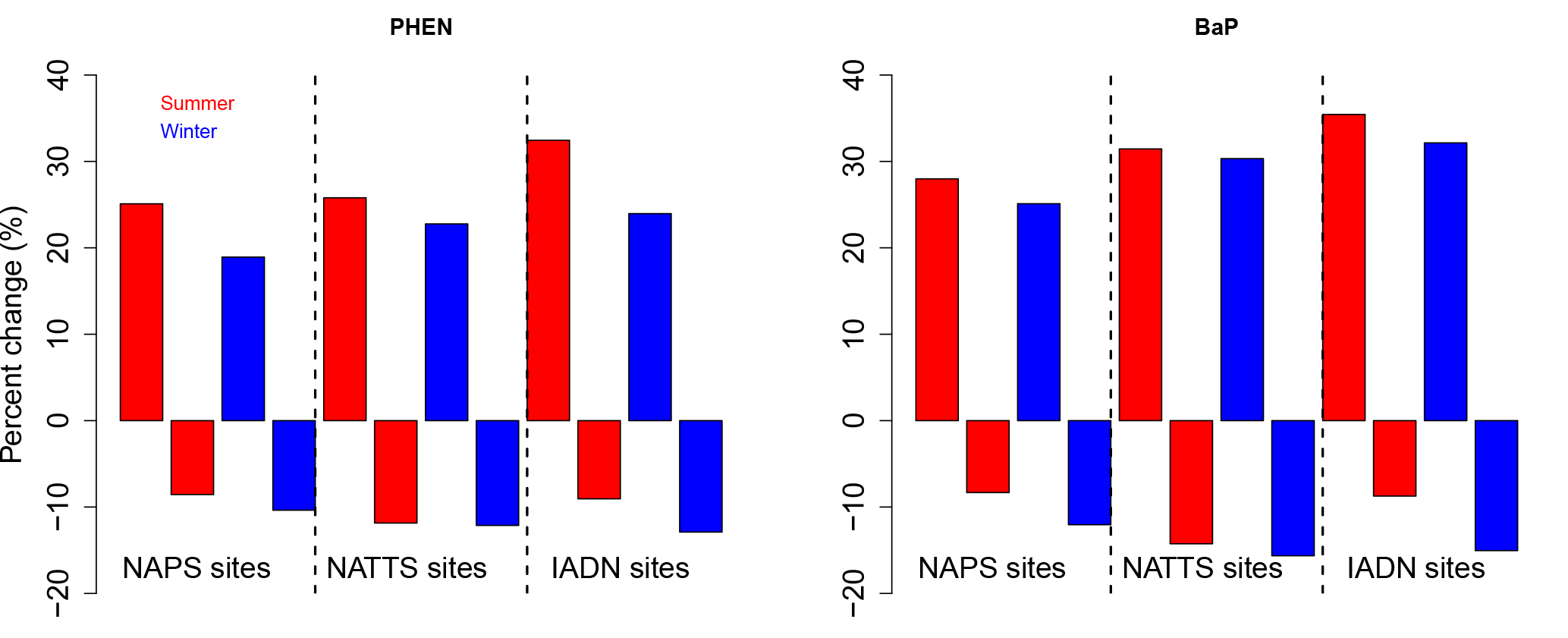
Figure 8Average percent change in surface PHEN and BaP concentrations by season when PAH on-road mobile emissions are scaled up or down by factors of 2.0 and 0.5, respectively.
4.3 Gas–particle partitioning of PAHs
The IADN network also allows us to assess model predictions of gas–particle partitioning of PAHs at six sites (24 h averages, every 6 days). Figure 9 shows a time series of pyrene particulate fraction (ϕk). Both model and measurements show higher ϕk in the wintertime, when there are higher PM concentrations for PAH adsorption, and lower temperatures. Generally, the model seems to underestimate ϕk at background sites (e.g., Burnt Island), and overestimate ϕk at urban sites (e.g, Chicago), and this is true for all PAH species. Thus, in Fig. 10, which shows the results for all PAHs at all sites, the model (green) has a larger range of ϕk than the measurements (orange). This is caused by the model overestimating and underestimating PM concentrations at urban and rural sites, respectively. For example, wind-blown dust is not included in the model; however, it is known to be a potentially significant contributor to total PM in rural areas. Also, due to an underestimate of vertical mixing in the model, PM tends to be biased high in urban areas, near emissions, due to a lack of a parameterization for urban heat islands (Stroud et al., 2012).
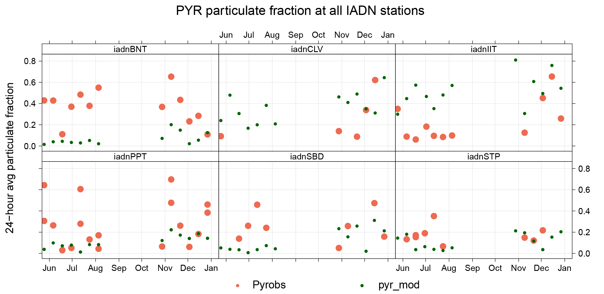
Figure 9Time series of pyrene particulate fraction at six IADN network sites (BNT represents Burnt Island, CLV represents Cleveland, IIT represents Chicago, PPT represents Point Petre, SBD represents Sleeping Bear Dunes, and STP represents Sturgeon Point). GEM-MACH-PAH values are denoted by (green dots) and IADN measurements by orange dots.
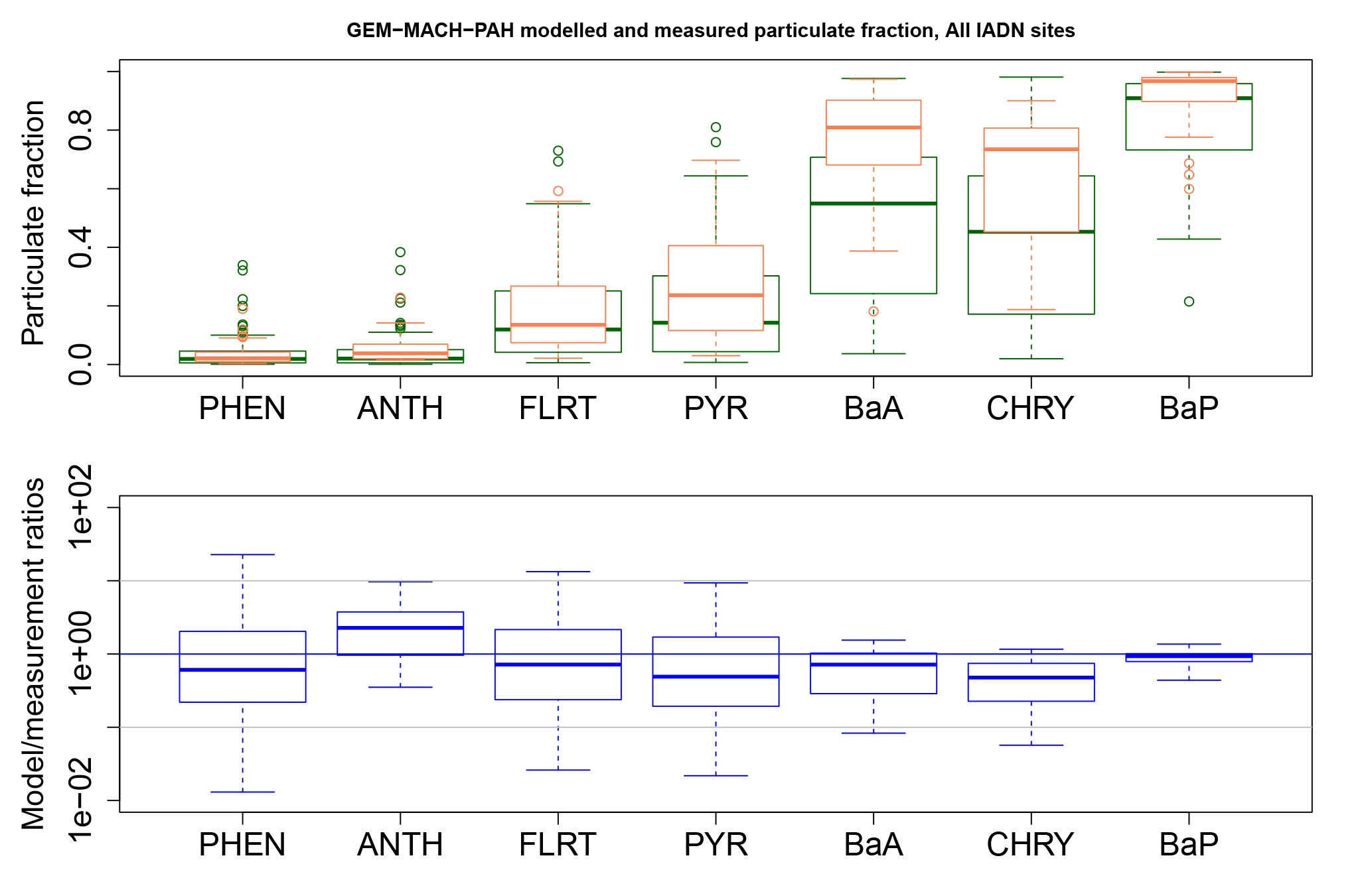
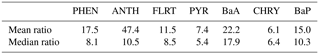
Figure 10GEM-MACH-PAH modelled (green) and measured (orange) particulate fraction (ϕ) of all PAHs at all IADN sites, and their model/measurement ratios (blue). The blue line indicates the one-to-one line, and the grey lines are for ratios of 10 and 0.1.
Comparing Fig. 10 (blue boxes) to Fig. 2b (green boxes), we see significant improvement over the original AURAMS-PAH partitioning due to the improved KSW parameters described in Sect. 2.2.1.
Generally, the gas–particle partitioning scheme in the model results in model/measurement ratios well within an order of magnitude, given by the gray lines in Fig. 10. ϕk for BaA and CHRY are still underestimated, but this may be related to modelled PM errors as noted earlier. We note that the addition of CTSP or even PM10 measurements at IADN sites (which existed in 2002, but not in 2009) would allow for the calculation of measured partitioning coefficients (logKp, Eq. 2), which could be used to validate the modelled logKp in future work. Since Kp takes total suspended particle into account, it removes the dependency on modelled PM; thus, it would increase confidence that the modelled partitioning is working properly, despite model errors in PM.
The fact that the GEM-MACH-PAH model partitioning of BaA and CHRY (and BaP to a lesser extent) puts too much concentration in the gas phase, may help explain why these species in particular are overestimated in the model. While in the gas phase, these species are less likely to be removed from the atmosphere, so their concentrations would erroneously build up in the model.
4.4 Wet deposition of PAHs
Table 2Mean and median GEM-MACH-PAH model/measurement ratios for PAH wet deposition.
When compared to the IADN 1-month wet deposition measurements, the model generally overestimates wet deposition for all PAHs, as is shown in Table 2 and Fig. 11. In Fig. 11, the blue lines show the ideal 1:1 model/measurement ratio, and most of the data lie well above these lines. By site (Fig. 11a), the modelled wet deposition was slightly better at urban locations (Toronto and Cleveland) than suburban and background sites (Burlington, Sturgeon Point, and Point Petre). By month (Fig. 11b), the wet deposition from the model is best represented in June and July, whereas, wet deposition is greatly overestimated in the winter, implying that the current snow adsorption parametrization may be too effective at removing PAHs in the model. This may be due to our simplification of a constant snow surface area, which may be set too high, or due to inaccuracies in the modelled or measured precipitation.
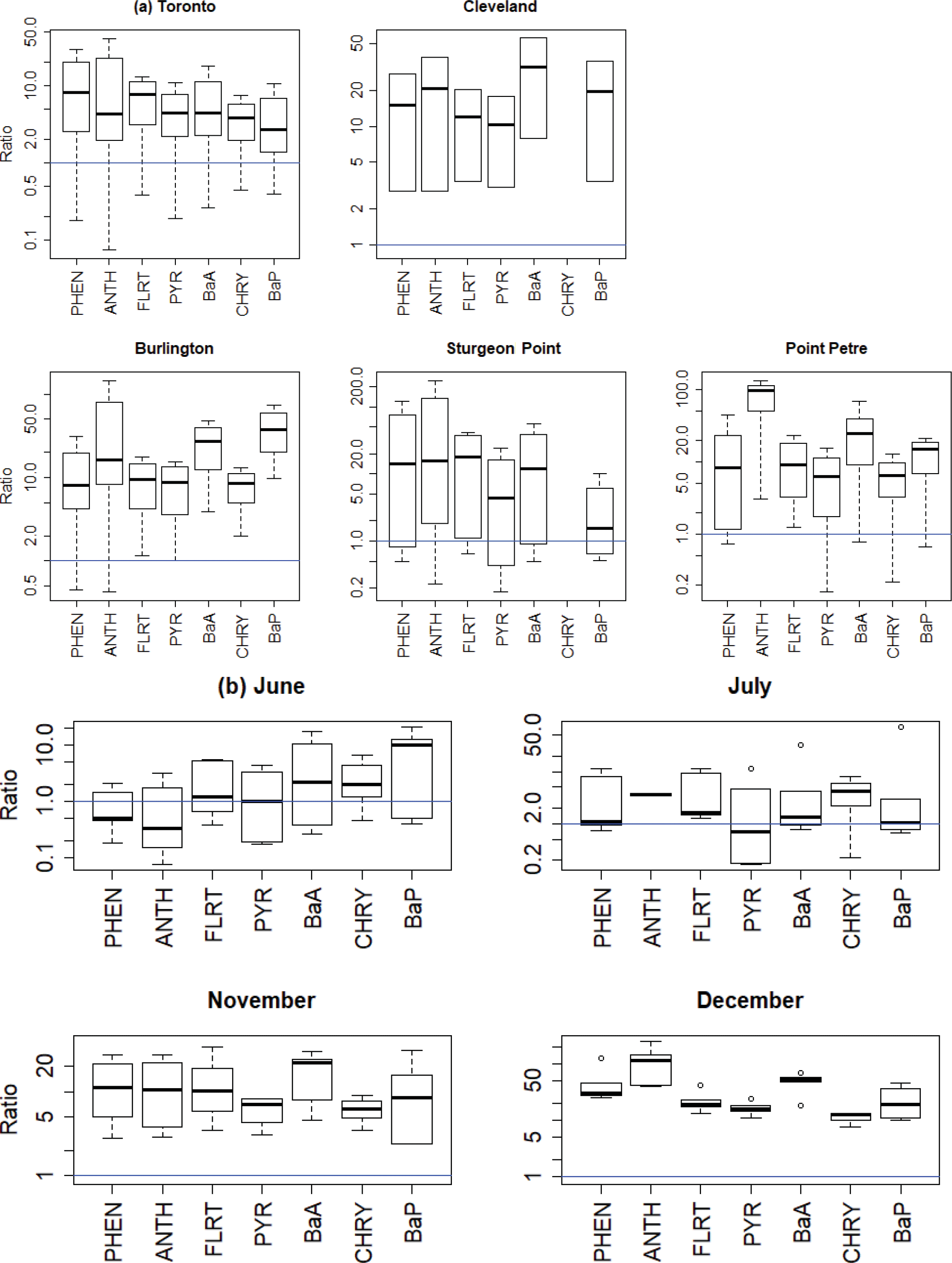
Figure 11GEM-MACH-PAH model/measurement wet deposition ratios for all PAHs (a) for five sites (all months) and (b) for four months (all IADN sites).
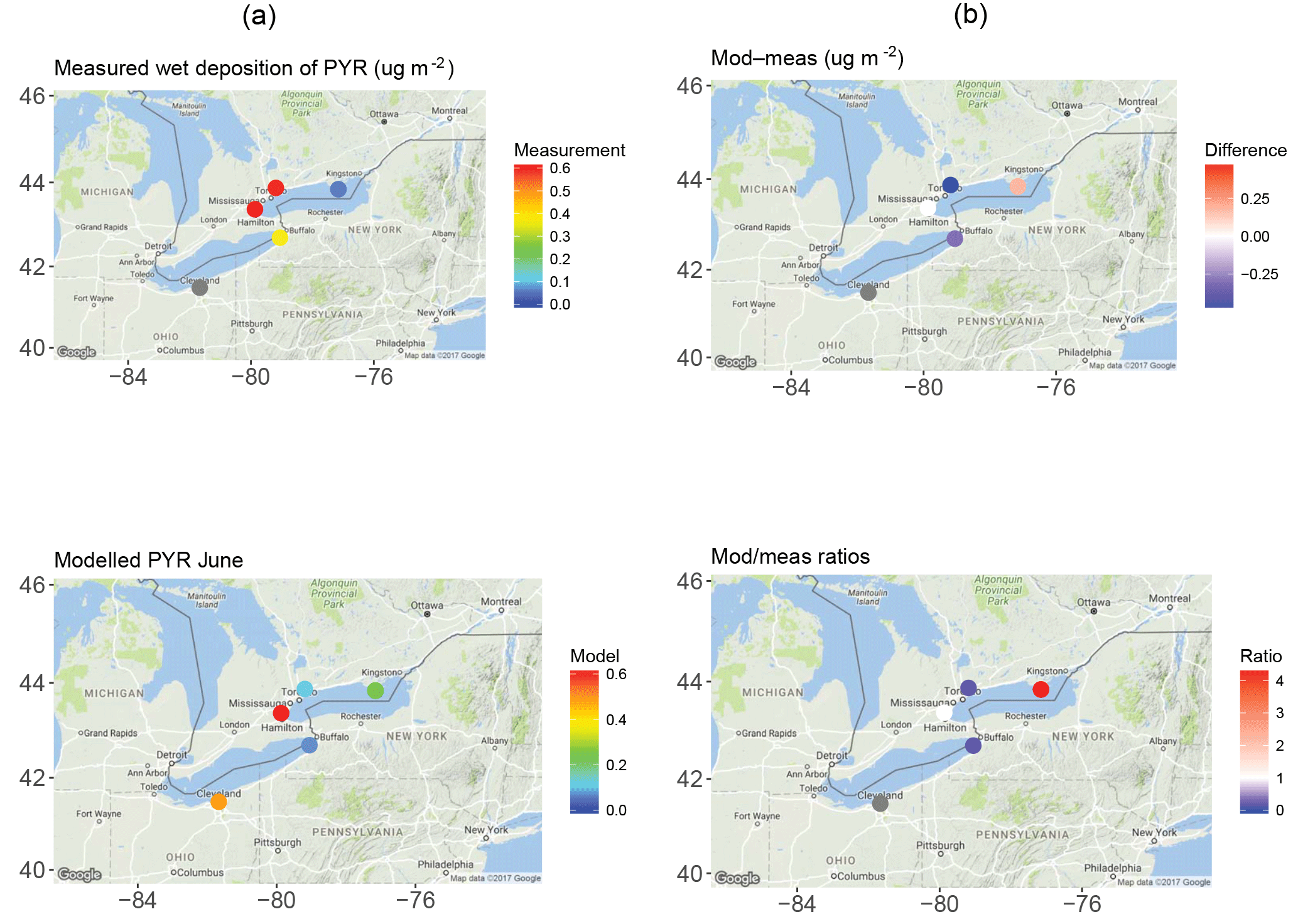
Figure 12One-month (June 2009) wet deposition of pyrene from the (a) measurements and GEM-MACH-PAH model and (b) their differences and ratios.
The IADN measurements, which report the concentration of PAHs in the collected precipitation (in pg L−1), were converted to pgPAH m−2 in order to compare to the wet deposition output of the model. However, this conversion assumes that the volume of precipitation reported by IADN was the total precipitation in the container's cross-sectional area, and in fact, it is not. The IADN wet deposition collectors are actually known to not sample all of the precipitation because the samplers are not in the correct configuration to get an accurate precipitation measurement (Dryfhout-Clark, personal communication, 2017). When we compared the actual precipitation amounts (from separate meteorological rain gauge data) to IADN precipitation volumes at the Point Petre location in January 2009, we found that only 68 % of the total precipitation was captured by the wet deposition sampler. Therefore, if that correction factor were applied to all IADN wet deposition measurements, they would increase by a factor of approximately 1.5, which would improve our comparison, but not eliminate the total bias. If IADN sites added separate, accurate rain gauges, then we could apply a “precipitation correction” to the IADN wet deposition measurements in a thorough, consistent way in future work.
Aside from the measurement bias, the modelled PAH wet deposition bias will also be dependent on the model's overall ability to predict accurate precipitation. We compared the modelled daily accumulated precipitation to the precipitation measured with the accurate gauges at Burnt Island and Point Petre, and found that, while the model's median precipitation bias was only about 0.2 mm, there was a large standard deviation, and there were some incidences where the model greatly over-predicted high precipitation events. Those incidences would result in greater modelled wet deposition of PAHs than was measured, and because we sum over a month, there is a significant likelihood of an over-prediction occurring in that long time frame. Indeed, the median ratios in Table 2, which are less sensitive to high outliers than the mean is, are substantially lower than the mean for most species.
Therefore, the model bias in wet deposition would appear to be caused by three additive factors: (1) measurements themselves having a negative bias relative to reality, due to insufficient capture of the net fluxes of precipitation; (2) modelled precipitation being biased high; and (3) a positive model bias in atmospheric PAH concentrations (which was highest for BaA and BaP in particular). Other PAH models have reported similar overestimates of PAH deposition (Matthias et al., 2009; Friedman and Selin, 2012).
The reverse reasoning can be applied, whereby we can see if high atmospheric concentrations of BaA and BaP were caused by too little wet deposition. In this case, since both of these species have correspondingly high wet deposition in the model (Fig. 11), it would appear that underestimation of wet deposition is probably not one of the causes.
Figure 12 shows results from a sample month (June 2009) for pyrene (PYR). The spatial distribution of wet deposition was not captured, with the model predicting lower PYR deposition in Toronto and Sturgeon Point than the measurements, higher at Point Petre, and about equal at Burlington. This spatial pattern is not the same for all PAHs, and even differs by month for the same PAH (e.g., PYR deposition in the next month, July, is low at Point Petre, high at Toronto, and highest in Burlington). The lack of spatial or temporal pattern in the sign and/or magnitude of wet deposition biases indicates that there is no major error with the PAH scavenging scheme itself. Given that wet deposition of PAHs relies on the correct simulation of many model factors (meteorology, scavenging parameters, atmospheric concentrations, etc.), our work suggests that more process studies aimed at quantifying wet deposition are needed. In fact, other PAH models also overestimate PAH deposition (Matthias et al., 2009; Friedman and Selin, 2012).
Through this work, a high-resolution chemical transport model for North American air toxics was created that allows us to see variations within a densely populated area. GEM-MACH-PAH was developed and run at a 2.5 km resolution for air quality forecasting and for simulating the impacts of emissions scenarios. Relative to AURAMS-PAH, on-road mobile emissions, gas–particle partitioning, and scavenging were all improved in this study. Mobile PAH emission factors from different sources were evaluated and the MOVES 2014 factors achieved the best model results compared to those in the recent literature and in the SPECIATE database. Parameters used in the gas–particle partitioning scheme (particularly KSW,k) were improved based on the observed relationship between logKp and logp, resulting in much better agreement between model and observations than was achieved with AURAMS-PAH. This is an important improvement because the gas–particle partitioning determines deposition and inhalation – both pathways of exposure in humans and ecosystems. Finally, we added snow scavenging, which was not a process included in AURAMS-PAH, and updated wet scavenging parameters. However, the modelled wet deposition was biased high – particularly in the wintertime – thus, further improvements to these parametrizations are required if the model is to be used for deposition studies.
Over the model domain, at seasonal timescales, the GEM-MACH-PAH simulation of benzene and six semi-volatile PAHs (PHEN, ANTH, FLRT, PYR, BaA, and CHRY) is statistically unbiased with respect to measurements (t<1 and p>0.05). For the seventh PAH species, BaP; its summertime average is simulated to a similar level of accuracy. However, it appears the model's OH, O3, and PM biases were additive, resulting in a wintertime average that is biased significantly high for BaP. Lack of removal of BaP via wet deposition was ruled out as a cause, but the lack of an O3 denuder system in the measurements contributes a small amount to the model–measurement differences as well. When we corrected BaP measurements using the Schauer et al. (2003) O3 relationship, we found reductions of about 20 % in the model/measurement ratios, improving the model performance.
Our results have shown that the major point source emissions play a large role in producing accurate model results near and downwind of industrial facilities, but also that the uncertainty associated with on-road mobile emission factors plays a large role in the accuracy of simulations near and within cities. In fact, we have determined from our sensitivity test that the GEM-MACH-PAH model has a linear response to a −50 to +100 % variation in mobile emission factors, simulating concentrations that vary up to 30 %. The spatial variability at high (2.5 km) resolution is modelled to within 50 % of Hamilton, Ontario measurements, although the model places higher concentrations in polluted areas, and lower concentrations in background areas than the measurements suggest, which is correlated to the spatial distribution of the model's PM bias. With this information, we can use the high-resolution GEM-MACH-PAH model for studying vehicle emissions scenarios in order to determine intra- and inter-city variations due to motor vehicles, with an understanding of the range of uncertainty that such a study would have.
Additional improvements to PAH modelling efforts could be achieved with general model improvements to its treatment of particulate matter (e.g., better parametrizations for wind-blown dust in rural areas, and better parametrizations for urban heat islands in urban areas). Also, additional reactions with particulate BaA and BaP in the model (e.g., with NO3 may reduce their bias further. It would also be beneficial to any future model/measurement studies, if the PAH measurement networks utilized ozone denuder technology so that particle-phase PAHs are not underestimated in the reported observations, as well as improved and consistent precipitation collection at wet deposition measurement sites. Partitioning could be better assessed if sites that measure PAH gas and particle phases separately (like IADN in this study) also measured CTSP or PM10. Finally, accurate emissions of PAHs at finer time and spatial resolutions could greatly improve model results.
Data availability: Please refer to Sect. 3 for the websites where the observations can be freely downloaded.
Model code availability: GEM-MACH – Atmospheric chemistry library for the GEM numerical atmospheric model Copyright © 2007–2013 – Air Quality Research Division and National Prediction Operations division, Environment and Climate Change Canada. This library is free software which can be redistributed and/or modified under the terms of the GNU Lesser General Public License as published by the Free Software Foundation; either version 2.1 of the License, or any later version. The MACH-PAH (chemistry) code can be downloaded from this Zenodo site: https://doi.org/10.5281/zenodo.1162252 (Whaley, 2018a), and the GEM (meteorology) code is available here: https://github.com/mfvalin?tab=repositories (Canadian Meteorological Centre, 2018). The executable for GEM-MACH-PAH is obtained by providing the chemistry library (MACH-PAH) to GEM when generating its executable.
The supplement related to this article is available online at: https://doi.org/10.5194/gmd-11-2609-2018-supplement.
CHW, EG, and PAM designed the experiments and CHW developed the model code with help from CS, WG, AA, and PAM. SG provided expertise on meteorological input and model simulation setup. EG and CS provided expertise on PAH and benzene subject matter. CHW carried out the simulations. JZ, QZ, and MDM developed the emissions input for the model and provided expertise about emissions. CHW prepared the manuscript with contributions from all co-authors.
The authors declare that they have no conflict of interest.
The authors gratefully acknowledge funding from ECCC's Climate Change and Air
Pollution program (CCAP, formerly called the Clean Air Regulatory Agenda).
Thank you to Angelos Anastasopolos and Amanda Wheeler for the Hamilton
measurement data, to Helena Dryfhout-Clark for consultation on IADN data
products, and Armaan Ladak for his help with the measurement data. Figures
were made using the R-based OpenAir package
(Carslaw and Ropkins, 2012; Carslaw, 2015).
Edited by: Astrid Kerkweg
Reviewed by: two anonymous referees
Agrawal, H., Welch, W. A., Miller, J. W., and Cocker, D. R.: Emissions Measurements from a Crude Oil Tanker at Sea, Environ. Sci. Technol., 42, 7098–7103, https://doi.org/10.1021/es703102y, 2008. a
Anastasopoulos, A. T., Wheeler, A. J., Karman, D., and Kulka, R. H.: Intraurban concentrations, spatial variability, and correlation of ambient polycyclic aromatic hydrocarbons (PAH) and PM2.5, Atmos. Environ., 59, 272–283, https://doi.org/10.1016/j.atmosenv.2012.05.004, 2012. a, b, c, d
Aulinger, A., Matthias, V., and Quante, M.: Introducing a partitioning mechanism for PAHs into the Community Multiscale Air Quality modeling system and its application to simulating the transport of benzo(a)pyrene over Europe, J. Appl. Meteorol. Clim., 46, 1718–1730, https://doi.org/10.1175/2007JAMC1395.1, 2007. a
Baklanov, A., Schlünzen, K., Suppan, P., Baldasano, J., Brunner, D., Aksoyoglu, S., Carmichael, G., Douros, J., Flemming, J., Forkel, R., Galmarini, S., Gauss, M., Grell, G., Hirtl, M., Joffre, S., Jorba, O., Kaas, E., Kaasik, M., Kallos, G., Kong, X., Korsholm, U., Kurganskiy, A., Kushta, J., Lohmann, U., Mahura, A., Manders-Groot, A., Maurizi, A., Moussiopoulos, N., Rao, S. T., Savage, N., Seigneur, C., Sokhi, R. S., Solazzo, E., Solomos, S., Sørensen, B., Tsegas, G., Vignati, E., Vogel, B., and Zhang, Y.: Online coupled regional meteorology chemistry models in Europe: current status and prospects, Atmos. Chem. Phys., 14, 317–398, https://doi.org/10.5194/acp-14-317-2014, 2014. a, b
Bidleman, T.: Atmospheric processes: wet and dry deposition of organic compounds are controlled by their vapor-particle partitioning, Environ. Sci. Technol., 22, 361–367, 1988. a
Bidleman, T. F. and Foreman, W. T.: Vapor-particle partitioning of semivolatile organic compounds, in: Sources and Fates of Aquatic Pollutants, American Chemical Society, 27–56, 1987. a
Blanchard, P., Audette, C. V., Hulting, M. L., Basu, I., Brice, K. A., Backus, S. M., Dryfhout-Clark, H., Froude, F., Hites, R. A., Neilson, M., and Wu, R.: Atmospheric deposition of toxic substances to the Great Lakes: IADN results through 2005, Report, Air Quality Research Division, Environment Canada; Great Lakes National Program Office, US EPA, 4905 Dufferin St., Toronto, ON, M3H 5T4, Canada, 77 West Jackson Blvd, Chicago, IL, 60604, USA, 2005. a, b, c
Brubaker, W. W. and Hites, R. A.: OH reaction kinetics of polycyclic aromatic hydrocarbons and polychlorinated dibenzo-p-dioxins and dibenzofurans, J. Phys. Chem., 102, 915–921, 1998. a
Bucheli, T. D. and Gustafsson, O.: Quantification of the soot-water distribution coefficient of PAHs provides mechanistic basis for enhanced sorption observations, Environ. Sci. Technol., 34, 5144–5151, https://doi.org/10.1021/es000092s, 2000. a, b, c, d
Canadian Meteorological Centre: gemdyn and rpnphy repositories, available at: https://github.com/mfvalin?tab=repositories, last access: 3 July 2018.
Carslaw, D. C.: The openair manual: open-source tools for analysing air pollution data, Technical report, available at: http://www.openair-project.org (last access: 3 July 2018), 2015. a
Carslaw, D. C. and Ropkins, K.: Openair: an R package for air quality data analysis, Environ. Modell. Softw., 27, 52–61, https://doi.org/10.1016/j.envsoft.2011.09.008, 2012. a
Chen, Y.-C., Lee, W.-J., Uang, S.-N., Lee, S.-H., and Tsai, P.-J.: Characteristics of polycyclic aromatic hydrocarbons (PAH) emissions from a UH-1H helicopter engine and its impact on the ambient environment, Atmos. Environ., 40, 7589–7597, https://doi.org/10.1016/j.atmosenv.2006.06.054, 2006. a
Côté, J., Desmarais, J.-G., Gravel, S., Méthot, A., Patoine, A., Roch, M., and Staniforth, A.: The Operational CMC–MRB Global Environmental Multiscale (GEM) Model. Part II: Results, Mon. Weather Rev., 126, 1397–1418, https://doi.org/10.1175/1520-0493(1998)126<1397:TOCMGE>2.0.CO;2, 1998a. a
Côté, J., Gravel, S., Méthot, A., Patoine, A., Roch, M., and Staniforth, A.: The Operational CMC–MRB Global Environmental Multiscale (GEM) Model. Part I: Design Considerations and Formulation, Mon. Weather Rev., 126, 1373–1395, https://doi.org/10.1175/1520-0493(1998)126<1373:TOCMGE>2.0.CO;2, 1998b. a
Dachs, J. and Eisenreich, S. J.: Adsorption onto aerosol soot carbon dominates gas-particle partitioning of polycyclic aromatic hydrocarbons, Environ. Sci. Technol., 34, 3690–3697, https://doi.org/10.1021/es991201, 2000. a, b, c, d, e, f, g
Daly, G. L. and Wania, F.: Simulating the influence of snow on the fate of organic compounds, Environ. Sci. Technol., 38, 4176–4186, https://doi.org/10.1021/es035105r, 2004. a
Dhammapala, R., Claiborn, C., Jimenez, J., Corkill, J., Gullett, B., Simpson, C., and Paulsen, M.: Emission factors of PAHs, methoxyphenols, levoglucosan, elemental carbon and organic carbon from simulated wheat and Kentucky bluegrass stubble burns, Atmos. Environ., 41, 2660–2669, https://doi.org/10.1016/j.atmosenv.2006.11.023, 2007. a, b
Domine, F., Taillandier, A.-S., and Simpson, W. R.: A parameterization of the specific surface area of seasonal snow for field use and for models of snowpack evolution, J. Geophys. Res., 112, F02031, https://doi.org/10.1029/2006JF000512, 2007. a
Dunbar, J. C., Lin, C. I., Vergucht, I., Wong, J., and Duran, J. L.: Estimating the contributions of mobile sources of PAH to urban air using real-time PAH monitoring, Sci. Total Environ., 279, 1–19, https://doi.org/10.1016/S0048-9697(01)00686-6, 2001. a
Eastern Research Group, Inc.: Technical Assistance document for the National Air Toxics Trends Stations Program – Revision 2, Report, Office of Air Quality Planning and Standards, US EPA, 601 Keystone Park Drive, Suite 700, Morrisville, NC 27560, 2009. a
Emmons, L. K., Walters, S., Hess, P. G., Lamarque, J.-F., Pfister, G. G., Fillmore, D., Granier, C., Guenther, A., Kinnison, D., Laepple, T., Orlando, J., Tie, X., Tyndall, G., Wiedinmyer, C., Baughcum, S. L., and Kloster, S.: Description and evaluation of the Model for Ozone and Related chemical Tracers, version 4 (MOZART-4), Geosci. Model Dev., 3, 43–67, https://doi.org/10.5194/gmd-3-43-2010, 2010. a
Environment Canada: 10 years of data from the National Air Pollution Surveillance (NAPS) network: DATA SUMMARY FROM 1999 to 2008, Report, Analysis and Air Quality Section, Air Quality Research Division, Science and Technology Branch, Toronto, ON, Canada, 2013. a
Franz, T. P. and Eisenreich, S. J.: Snow scavenging of polychlorinated biphenyls and polycyclic aromatic hydrocarbons in Minnesota, Environ. Sci. Technol., 32, 1771–1778, https://doi.org/10.1021/es970601z, 1998. a, b, c
Friedman, C. L. and Selin, N. E.: Long-range atmospheric transport of polycyclic aromatic hydrocarbons: a global 3-D model analysis including evaluation of Arctic sources, Environ. Sci. Technol., 46, 9501–9510, https://doi.org/10.1021/es301904d, 2012. a, b, c, d, e, f
Galarneau, E., Makar, P. A., Sassi, M., and Diamond, M. L.: Estimation of Atmospheric Emissions of Six Semivolatile Polycyclic Aromatic Hydrocarbons in Southern Canada and the United States by Use of an Emissions Processing System, Environ. Sci. Technol., 41, 4205–4213, https://doi.org/10.1021/es062303k, 2007. a, b, c, d, e, f, g, h
Galarneau, E., Makar, P. A., Zheng, Q., Narayan, J., Zhang, J., Moran, M. D., Bari, M. A., Pathela, S., Chen, A., and Chlumsky, R.: PAH concentrations simulated with the AURAMS-PAH chemical transport model over Canada and the USA, Atmos. Chem. Phys., 14, 4065–4077, https://doi.org/10.5194/acp-14-4065-2014, 2014. a, b, c, d, e, f, g, h, i, j
Galarneau, E., Wang, D., Dabek-Zlotorzynska, E., Siu, M., Celo, V., Tardif, M., Harnish, D., and Jiang, Y.: Air toxics in Canada measured by the National Air Pollution Surveillance (NAPS) Program and their relation to ambient air quality guidelines, JAPCA J. Air Waste Ma., 66, 184–200, https://doi.org/10.1080/10962247.2015.1096863, 2016. a, b, c
Gariazzo, C., Silibello, C., Finardi, S., Radice, P., Pieranti, A., Calori, G., Cecinato, A., Perrino, C., Nussio, F., Cagnoli, M., Pelliccioni, A., Gobbi, G. P., and Filippo, P. D.: A gas aerosol air pollutants study over the urban area of Rome using a comprehensive chemical transport model, Atmos. Environ., 41, 7286–7303, https://doi.org/10.1016/j.atmosenv.2007.05.018, 2007. a
Gong, W., Dastoor, A., Bouchet, V., Gong, S., Makar, P., Moran, M., Pabla, B., Ménard, S., Crevier, L.-P., Cousineau, S., and Venkatesh, S.: Cloud processing of gases and aerosols in a regional air quality model (AURAMS), Atmos. Res., 82, 248–275, 2006. a
Gong, W., Makar, P. A., Zhang, J., Milbrandt, J., Gravel, S., Hayden, K. L., Macdonald, A. M., and Leaitch, W. R.: Modelling aerosol cloud meteorology interaction: A case study with a fully coupled air quality model GEM-MACH, Atmos. Environ., 115, 695–715, https://doi.org/10.1016/j.atmosenv.2015.05.062, 2015. a
Goriaux, M., Jourdain, B., Temime, B., Besombes, J.-L., Marchand, N., Albinet, A., Leoz-Garziandia, E., and Wortham, H.: Field comparison of particulate PAH measurements using a low-flow denuder device and conventional sampling systems, Environ. Sci. Technol., 40, 6398–6404, https://doi.org/10.1021/es060544m, 2006. a
Hachikubo, A., Yamaguchi, S., Arakawa, H., Tanikawa, T., Hori, M., Sugiura, K., Matoba, S., Niwano, M., Kuchiki, K., and Aoki, T.: Effects of temperature and grain type on time variation of snow specific surface area, Bull. Glac. Res., 32, 47–53, https://doi.org/10.5331/bgr.32.47, 2014. a
Hall, D., Wu, C.-Y., Hsu, Y.-M., Stormer, J., Engling, G., Capeto, K., Wang, J., Brown, S., Li, H.-W., and Yu, K.-M.: PAHs, cabonyls, VOCs and PM2.5 emission factors for pre-harvest burning of Florida surgarcane, Atmos. Environ., 55, 164–172, https://doi.org/10.1016/j.atmosenv.2012.03.034, 2012. a, b
Hanot, L. and Dominé, F.: Evolution of the surface area of a snow layer, Environ. Sci. Technol., 33, 4250–4255, https://doi.org/10.1021/es9811288, 1999. a
Hoff, J. T., Gregor, D., Mackay, D., Wania, F., and Jia, C. Q.: Measurement of the specific surface area of snow with the nitrogen adsorption technique, Environ. Sci. Technol., 32, 58–62, https://doi.org/10.1021/es970225i, 1998. a
Jariyasopit, N., Zimmermann, K., Schrlau, J., Arey, J., Atkinson, R., Yu, T.-W., Dashwood, R. H., Tao, S., and Simonisch, S. L. M.: Heterogeneous reaction of particulate matter-bound PAHs and NPAHs with NO3∕N2O5, OH radicals and O3 under simulated long-range atmospheric transport conditions: reactivity and mutagenicity, Environ. Sci. Technol., 48, 10155–10164, https://doi.org/10.1021/es5015407, 2014. a
Joe, P., Belair, S., Bernier, N. B., Bouchet, V., Brook, J. R., Brunet, D., Burrows, W., Charland, J. P., Dehghan, A., Driedger, N., Duhaime, C., Evans, G., Filion, A.-B., Frenette, R., de Granpré, J., Guiltepe, I., Henderson, D., Herdt, A., Hilker, N., Huang, L., Hung, E., Isaac, G., Jeong, C.-H., Johnston, D., Klaassen, J., Leroyer, S., Lin, H., MacDonald, M., MacPhee, J., Mariani, Z., Munoz, T., Reid, J., Robichaud, A., Rochon, Y., Shairsingh, K., Sills, D., Spacek, L., Stroud, C., Su, Y., Taylor, N., Vanos, J., Voogt, J., Wang, J. M., Wiechers, T., Wren, S., Yang, H., and Yip, T.: The Environment Canada Pan and ParaPan American Science Showcase Project, B. Am. Meteorol. Soc., 921–953, https://doi.org/10.1175/BAMS-D-16-0162.1, 2017. a
Jonker, M. T. O. and Koelmans, A. A.: Sorption of polycyclic aromatic hydrocarbons and polychrorinated biphenyls to soot and soot-like materials in the aqueous environment: mechanistic considerations, Environ. Sci. Technol., 36, 3725–3734, https://doi.org/10.1021/es020019x, 2002. a, b, c, d, e, f, g
Junge, C. E.: Basic considerations about trace constituents in the atmosphere as related to the fate of global pollutants, in: Fate of pollutants in the air and water environments, edited by: Suffet, I. H., Wiley, New York, 7–25, 1977. a, b
Kahan, T. F., Kwamena, N.-O., and Donaldson, D. J.: Heterogeneous ozonation kinetics of polycyclic aromatic hydrocarbons on organic films, Atmos. Environ., 40, 3448–3459, 2006. a, b
Keyte, I. J., Harrison, R. M., and Lammel, G.: Chemical reactivity and long-range transport potential of polycyclic aromatic hydrocarbons - a review, Chem. Soc. Rev., 42, 9333–9392, https://doi.org/10.1039/c3cs60147a, 2013. a, b, c, d
Khalek, I. A., Bougher, T. L., and Merritt, P. M.: Phase 1 of the advanced collaborative emissions study, Report, Coordinating Research Council, INC., Mansell Rd, Alpharetta, GA, USA, 30022, 2009. a
Kim, K., Jahan, S., Kabir, E., and Brown, R. J.: A review of airborne polycyclic aromatic hydrocarbons (PAHs) and their human health effects, Environ. Int., 60, 71–80, https://doi.org/10.1016/j.envint.2013.07.019, 2013. a
Kishan, S., Crews, W., Zmud, M., Fujita, E., Burnette, A., Snow, R., Santos, R., Campbell, D., Fincher, S., Bricka, S., Arnott, P., and Sabisch, M.: Kansas City PM characterization study: Final Report, Report, Assessment and Standards Division, Office of Transportation and Air Quality, U.S. EPA, and the Eastern Research Group Inc., 5608 Parkcrest Drive Suite 100, Austin, TX, USA, 2008. a
Kuoppamäki, K., Setälä, H., Rantalainen, A.-L., and Kotze, D. J.: Urban snow indicates pollution originating from road traffic, Environ. Pollut., 195, 56–63, https://doi.org/10.1016/j.envpol.2014.08.019, 2014. a
Kwamena, N.-O., Thornton, J. A., and Abbatt, J. P. D.: Kinetics of surface-bound benzo(a)pyrene and ozone on solid organic and salt aerosols, J. Phys. Chem., 108, 11626–11634, https://doi.org/10.1021/jp046161x, 2004. a, b
Kwamena, N.-O. A., Staikova, M. G., Donaldson, D. J., George, I. J., and Abbatt, J. P. D.: Role of the Aerosol Substrate in the Heterogeneous Ozonation Reactions of Surface-Bound PAHs, J. Phys. Chem., 111, 11050–11058, https://doi.org/10.1021/jp075300i, 2007. a
Lei, Y. D. and Wania, F.: Is rain or snow a more efficient scavenger of organic chemicals?, Atmos. Environ., 38, 3557–3571, https://doi.org/10.1016/j.atmosenv.2004.03.039, 2004. a, b
Liu, C., Zhang, P., Yang, B., Wang, Y., and Shu, J.: Kinetic studies of heterogeneous reactions of polycyclic aromatic hydrocarbon aerosols with NO3 radicals, Environ. Sci. Technol., 46, 7575–7580, https://doi.org/10.1021/es301403d, 2012. a
Liu, K., Duan, F., He, K., Ma, Y., and Cheng, Y.: Investigation on sampling artefacts of particle associated PAHs using ozone denuder systems, Front. Environ. Sci. En., 8, 284–292, https://doi.org/10.1007/s11783-013-0555-7, 2014. a, b, c, d
Lohmann, R. and Lammel, G.: Adsorptive and Absorptive Contributions to the Gas-Particle Partitioning of Polycyclic Aromatic Hydrocarbons: State of Knowledge and Recommended Parametrization for Modeling, Environ. Sci. Technol., 38, 3793–3803, https://doi.org/10.1021/es035337q, 2004. a
Ma, Y.-G., Lei, Y. D., Xiao, H., Wania, F., and Wang, W.-H.: Critical review and recommended values for the physical-chemical property data of 15 polycyclic aromatic hydrocarbons at 25 ∘C, J. Chem. Eng. Data, 55, 819–825, https://doi.org/10.1021/je900477x, 2010. a
Makar, P. A., Zhang, J., Gong, W., Stroud, C., Sills, D., Hayden, K. L., Brook, J., Levy, I., Mihele, C., Moran, M. D., Tarasick, D. W., He, H., and Plummer, D.: Mass tracking for chemical analysis: the causes of ozone formation in southern Ontario during BAQS-Met 2007, Atmos. Chem. Phys., 10, 11151–11173, https://doi.org/10.5194/acp-10-11151-2010, 2010. a, b
Makar, P. A., Gong, W., Hogrefe, C., Zhang, Y., Curci, G., Zabkar, R. ., Milbrandt, J., Im, U., Balzarini, A., Baró, R., Bianconi, R., Cheung, P., Forkel, R., Gravel, S., Hirtl, M., Honzak, L., Hou, A., Jiménez-Guerrero, P., Langer, M., Moran, M., Pabla, B., Pérez, J., Pirovano, G., José, R. S., Tuccella, P., Werhahn, J., Zhang, J., and Galmarini, S.: Feedbacks between air pollution and weather, part 2: Effects on chemistry, Atmos. Environ., 115, 499–526, https://doi.org/10.1016/j.atmosenv.2014.10.021, 2015a. a
Makar, P. A., Gong, W., Milbrandt, J., Hogrefe, C., Zhang, Y., Curci, G., Zabkar, R. ., Im, U., Balzarini, A., Baró, R., Bianconi, R., Cheung, P., Forkel, R., Gravel, S., Hirtl, M., Honzak, L., Hou, A., Jiménez-Guerrero, P., Langer, M., Moran, M., Pabla, B., Pérez, J., Pirovano, G., José, R. S., Tuccella, P., Werhahn, J., Zhang, J., and Galmarini, S.: Feedbacks between air pollution and weather, part 1: Effects on weather, Atmos. Environ., 115, 442–469, https://doi.org/10.1016/j.atmosenv.2014.12.003, 2015b. a
Makar, P. A., Akingunola, A., Aherne, J., Cole, A. S., Aklilu, Y.-A., Zhang, J., Wong, I., Hayden, K., Li, S.-M., Kirk, J., Scott, K., Moran, M. D., Robichaud, A., Cathcart, H., Baratzedah, P., Pabla, B., Cheung, P., Zheng, Q., and Jeffries, D. S.: Estimates of Exceedances of Critical Loads for Acidifying Deposition in Alberta and Saskatchewan, Atmos. Chem. Phys. Discuss., https://doi.org/10.5194/acp-2017-1094, in review, 2018. a
Matthias, V., Aulinger, A., and Quante, M.: CMAQ simulations of the benzo(a)pyrene distribution over Europe for 2000 and 2001, Atmos. Environ., 43, 4078–4086, https://doi.org/10.1016/j.atmosenv.2009.04.058, 2009. a, b
Menichini, E.: On-filter degradation of particle-bound benzo(a)pyrene by ozone during air sampling: a review of the experimental evidence of an artefact, Chemosphere, 77, 1275–1284, https://doi.org/10.1016/j.chemosphere.2009.09.019, 2009. a, b, c, d
Miao, Q., Bouchard, M., Chen, D., Rosenberg, M. W., and Aronson, K. J.: Commuting behaviors and exposure to air pollution in Montreal, Canada, Sci. Total Environ., 508, 193–198, https://doi.org/10.1016/j.scitotenv.2014.11.078, 2015. a
Moran, M., Menard, S., Gravel, S., Pavlovic, R., and Anselmo, D.: RAQDPS Versions 1.5.0 and 1.5.1: Upgrades to the CMC Operational Regional Air Quality Deterministic Prediction System Released in October 2012 and February 2013, Technical report, Canadian Meteorological Centre, Canadian Meteorological Centre, Dorval, Quebec, 2013. a
Moran, M. D., Ménard, S., Talbot, D., Huang, P., Makar, P. A., Gong, W., Landry, H., Gravel, S., Gong, S., Crevier, L.-P., Kallaur, A., and Sassi, M.: Particulate-matter forecasting with GEM-MACH15, a new Canadian air-quality forecast model, in: Air pollution modelling and its application XX, edited by: Steyn, D. G. and Rao, S. T., Springer, Dordrecht, 289–292, 2010. a, b
Mu, Q., Shiraiwa, M., Octaviani, M., Ma, N., Ding, A., Su, H., Lammel, G., Pöschl, U., and Cheng, Y.: Temperature effect on phase state and reactivity controls atmospheric multiphase chemistry and transport of PAHs, Sci. Adv., 4, eaap7314, https://doi.org/10.1126/sciadv.aap7314, 2018. a, b
Odabasi, M., Bayram, A., Elbir, T., Seyfioglu, R., Dumanoglu, Y., Bozlaker, A., Demircioglu, H., Altiok, H., Yatkin, S., and Cetin, B.: Electric Arc Furnaces for Steel-Making: Hot Spots for Persistent Organic Pollutants, Environ. Sci. Technol., 43, 5205–5211, https://doi.org/10.1021/es900863s, 2009. a
Okochi, H., Sugimoto, D., and Igawa, M.: The enhanced dissolution of some chlorinated hydrocarbons and monocyclic aromatic hydrocarbons in rainwater collected in Yokohama, Japan, Atmos. Environ., 38, 4403–4414, https://doi.org/10.1016/j.atmosenv.2004.03.053, 2004. a
Pachón, J. E., Sarmiento, H., and Hoshiko, T.: Health risk represented by inhaling polycyclic aromatic hydrocarbons (PAH) during daily commuting involving using a high traffic flow route in Bogotá, Rev. Salud Publica (Bogota), 3, 198–407, 2013. a
Pankow, J. F.: Review and comparative analysis of the theories on partitioning between the gas and aerosol particulate phases in the atmosphere, Atmos. Environ., 21, 2275–2283, https://doi.org/10.1016/0004-6981(87)90363-5, 1987. a, b
Pendlebury, D., Gravel, S., Moran, M., and Lupu, A.: The impact of chemical lateral boundary conditions in a regional air quality forecast model on surface ozone predictions during stratospheric intrusions, Atmos. Environ., https://doi.org/10.1016/j.atmosenv.2017.10.052, 2017. a
Pitts Jr., J., Paur, H.-R., Zielinska, B., Arey, J., Winer, A., Ramdahl, T., and Mejia, V.: Factors influencing reactivity of polycyclic aromatic hydrocarbons adsorbed on filters and ambient POM with ozone, Chemosphere, 15, 675–685, https://doi.org/10.1016/0045-6535(86)90033-0, 1986. a
Pöschl, U., Letzel, T., Schauer, C., and Niessner, R.: Interaction of ozone and water vapor with spark discharge soot aerosol particles coated with benzo(a)pyrene: O3 and H2O adsportion, benzo(a)pyrene degradation, and atmospheric implications, J. Phys. Chem., 105, 4029–4041, 2001. a, b
Ringuet, J., Albinet, A., Leoz-Garzandia, E., Budzinski, H., and Villenava, E.: Reactivity of polycyclic aromatic compounds (PAHs, NPAHs, and OPAHs) adsorbed on natural aerosol particles exposed to atmospheric oxidants, Atmos. Environ., 61, 15–22, https://doi.org/10.1016/j.atmosenv.2012.07.025, 2012. a, b
Samaali, M., Moran, M., Bouchet, V., Pavlovic, R., Cousineau, S., and Sassi, M.: On the influence of chemical initial and boundary conditions on annual regional air quality model simulations for North America, Atmos. Environ., 43, 4873–4885, 2009. a, b
Sander, R.: Modeling atmospheric chemistry: interactions between gas-phase species and liquid cloud/aerosol particles, Surv. Geophys., 20, 1–31, 1999. a
Schauer, C., Neissner, R., and Pöschl, U.: Polycyclic aromatic hydrocarbons in urban air particulate matter: decadal and seasonal trends, chemical degradation, and sampling artifacts, Environ. Sci. Technol., 37, 2861–2868, https://doi.org/10.1021/es034059s, 2003. a, b
Skrdlíková, L., Landlová, L., Klánová, J., and Lammel, G.: Wet deposition and scavenging efficiency of gaseous and particulate phase polycyclic aromatic compounds at a central European suburban site, Atmos. Environ., 45, 4305–4312, https://doi.org/10.1016/j.atmosenv.2011.04.072, 2011. a
Smith, D. J. T. and Harrison, R. M.: Concentrations, trends and vehicle source profile of polynuclear aromatic hydrocarbons in the U.K. atmosphere, Atmos. Environ., 30, 2513–2525, https://doi.org/10.1080/10962247.2015.1096863, 1996. a
Stroud, C. A., Moran, M. D., Makar, P. A., Gong, S., Gong, W., Zhang, J., Slowik, J. G., Abbatt, J. P. D., Lu, G., Brook, J. R., Mihele, C., Li, Q., Sills, D., Strawbridge, K. B., McGuire, M. L., and Evans, G. J.: Evaluation of chemical transport model predictions of primary organic aerosol for air masses classified by particle component-based factor analysis, Atmos. Chem. Phys., 12, 8297–8321, https://doi.org/10.5194/acp-12-8297-2012, 2012. a, b, c
Thackray, C. P., Friedman, C. L., Zhang, Y., and Selin, N. E.: Quantitative Assessment of Parametric Uncertainty in Northern Hemisphere PAH Concentrations, Environ. Sci. Tech. Let., 49, 9185–9193, https://doi.org/10.1021/acs.est.5b01823, 2015. a
Umwelterhebungen and Gerätesichereit: Ozone Cross-sensitivity by the Emmission Measurements of Suspended-particles Accumulated Benzo(a)-pyrene, Umeg report no. 33-02-2002, english version, Assessment and Standards Division, Office of Transportation and Air Quality, U.S. EPA, and the Eastern Research Group Inc., Zentrum für Umweltmessungen, Umwelterhebungen und Gerätesicherheit, Karlsruhe, Germany, 2002. a
US EPA: AP 42, Fifth Edition, Compilation of Air Pollutant Emission Factors, Volume 1: Stationary Point and Area Sources, Report, Office of Air Quality Planning and Standards, Office of Air and Radiation, Research Triangle Park, NC, 27711, USA, 1995. a
US EPA: Locating and estimating air emissions from sources of polycyclic organic matter, Report epa-454/r-98-014, US EPA, OAQPS, Washington, DC, 1998. a
US EPA: National Air Toxics Trends Stations quality assurance annual report calendar year 2009 – Final, Report, Office of Air Quality Planning and Standards, Research Triangle Park, NC 27711, USA, 2009. a
Wang, X., Zhang, L., and Moran, M. D.: Uncertainty assessment of current size-resolved parameterizations for below-cloud particle scavenging by rain, Atmos. Chem. Phys., 10, 5685–5705, https://doi.org/10.5194/acp-10-5685-2010, 2010. a
Wania, R., Mackay, D., and Hoff, J. T.: The importance of snow scavenging of polychlorinated biphenyls and polycyclic aromatic hydrocarbon vapors, Environ. Sci. Technol., 33, 195–197, https://doi.org/10.1021/es980806n, 1999. a
Wesely, M. L.: Parameterization of surface resistances to gaseous dry deposition in regional-scale numerical models, Atmos. Environ., 23, 1293–1304, https://doi.org/10.1016/0004-6981(89)90153-4, 1989. a
Whaley, C., Galarneau, E., Makar, P. A., Moran, M. D., Stroud, C., Gong, W., and Gravel, S.: GEM-MACH-PAH, rev2488, https://doi.org/10.5281/zenodo.1162252, 2018a.
Whaley, C. H., Makar, P. A., Shephard, M. W., Zhang, L., Zhang, J., Zheng, Q., Akingunola, A., Wentworth, G. R., Murphy, J. G., Kharol, S. K., and Cady-Pereira, K. E.: Contributions of natural and anthropogenic sources to ambient ammonia in the Athabasca Oil Sands and north-western Canada, Atmos. Chem. Phys., 18, 2011–2034, https://doi.org/10.5194/acp-18-2011-2018, 2018b. a
Xu, H.-Y., Zou, J.-W., Min, J.-Q., and Wang, W.: A quantitative structure–property relationship analysis of soot–water partition coefficients for persistent organic pollutants, Ecotox. Environ. Safety, 80, 1–5, https://doi.org/10.1016/j.ecoenv.2012.02.002, 2012. a, b, c, d
Yamasaki, H., Kuwata, K., and Miyamoto, H.: Effects of ambient temperature on aspects of airborne polycyclic aromatic hydrocarbons, Environ. Sci. Technol., 16, 189–194, https://doi.org/10.1021/es00098a003, 1982. a
Zhang, J., Wang, P., Li, J., Mendola, P., Sherman, S., and Ying, Q.: Estimating population exposure to ambient polycyclic aromatic hydrocarbon in the United States – Part II: Source apportionment and cancer risk assessment, Environ. Int., 97, 163–170, https://doi.org/10.1016/j.envint.2016.08.024, 2016. a, b
Zhang, J., Li, J., Wang, P., Chen, G., Mendola, P., Sherman, S., and Ying, Q.: Estimating population exposure to ambient polycyclic aromatic hydrocarbon in the United States – Part I: Model development and evaluation, Environ. Int., 99, 263–274, https://doi.org/10.1016/j.envint.2016.12.002, 2017. a, b
Zhang, L., Gong, S., Padro, J., and Barrie, L.: A size-segregated particle dry deposition 270 scheme for an atmospheric aerosol module, Atmos. Environ., 35, 549–560, 2001. a
Zhang, L., Moran, M., Makar, P., Brook, J., and Gong, S.: Gaseous Dry Deposition in AURAMS A Unified Regional Air-quality Modelling System, Atmos. Environ., 36, 537–560, https://doi.org/10.1016/S1352-2310(01)00447-2, 2002. a