the Creative Commons Attribution 3.0 License.
the Creative Commons Attribution 3.0 License.
Plume-SPH 1.0: a three-dimensional, dusty-gas volcanic plume model based on smoothed particle hydrodynamics
Zhixuan Cao
Abani Patra
Marcus Bursik
E. Bruce Pitman
Matthew Jones
Plume-SPH provides the first particle-based simulation of volcanic plumes. Smoothed particle hydrodynamics (SPH) has several advantages over currently used mesh-based methods in modeling of multiphase free boundary flows like volcanic plumes. This tool will provide more accurate eruption source terms to users of volcanic ash transport and dispersion models (VATDs), greatly improving volcanic ash forecasts. The accuracy of these terms is crucial for forecasts from VATDs, and the 3-D SPH model presented here will provide better numerical accuracy. As an initial effort to exploit the feasibility and advantages of SPH in volcanic plume modeling, we adopt a relatively simple physics model (3-D dusty-gas dynamic model assuming well-mixed eruption material, dynamic equilibrium and thermodynamic equilibrium between erupted material and air that entrained into the plume, and minimal effect of winds) targeted at capturing the salient features of a volcanic plume. The documented open-source code is easily obtained and extended to incorporate other models of physics of interest to the large community of researchers investigating multiphase free boundary flows of volcanic or other origins.
The Plume-SPH code (https://doi.org/10.5281/zenodo. 572819) also incorporates several newly developed techniques in SPH needed to address numerical challenges in simulating multiphase compressible turbulent flow. The code should thus be also of general interest to the much larger community of researchers using and developing SPH-based tools. In particular, the SPH−ε turbulence model is used to capture mixing at unresolved scales. Heat exchange due to turbulence is calculated by a Reynolds analogy, and a corrected SPH is used to handle tensile instability and deficiency of particle distribution near the boundaries. We also developed methodology to impose velocity inlet and pressure outlet boundary conditions, both of which are scarce in traditional implementations of SPH.
The core solver of our model is parallelized with the message passing interface (MPI) obtaining good weak and strong scalability using novel techniques for data management using space-filling curves (SFCs), object creation time-based indexing and hash-table-based storage schemes. These techniques are of interest to researchers engaged in developing particles in cell-type methods. The code is first verified by 1-D shock tube tests, then by comparing velocity and concentration distribution along the central axis and on the transverse cross with experimental results of JPUE (jet or plume that is ejected from a nozzle into a uniform environment). Profiles of several integrated variables are compared with those calculated by existing 3-D plume models for an eruption with the same mass eruption rate (MER) estimated for the Mt. Pinatubo eruption of 15 June 1991. Our results are consistent with existing 3-D plume models. Analysis of the plume evolution process demonstrates that this model is able to reproduce the physics of plume development.


1.1 Volcanic ash hazards
Primary hazards associated with explosive volcanic eruptions include pyroclastic density currents (flows and surges), the widespread deposition of air fall tephra and the threats to aviation posed by volcanic ash in the atmosphere. Simulation of all possible hazards with one model is difficult due to the fact that different length scales dominate different hazards. Our focus here is the hazard that volcanic ash poses to aircraft.
During volcanic eruptions, volcanic ash transport and dispersion models (VATDs) are used to forecast the location and movement of ash clouds at timescales that range from hours to days. VATDs use eruption source parameters, such as plume height, mass eruption rate, duration and the mass fraction distribution of erupted particles finer than about 4Φ (or 62.5 µm), which can remain in the cloud for many hours or days. Observational data for such parameters are usually unavailable in the first minutes or hours after an eruption is detected. Moreover, these input parameters are subject to change during an eruption, requiring rapid reassignment of new parameters. Usually, plume models are used to provide these source terms for VATDs and the forecast accuracy is critically dependent on these models. This paper reports on a new three-dimensional (3-D) volcanic plume model designed to exploit the advantages of mesh-free methods for 3-D modeling of such plumes that involve multiphase free boundary flows.
1.2 Existing plume models
Several one-dimensional (1-D) volcanic plume models have been developed in the past few decades, ranging from the most basic 1-D model (Woods, 1988) which only accounts for mass conservation to more recently developed 1-D models (Bursik, 2001; Mastin, 2007; Degruyter and Bonadonna, 2012; Woodhouse et al., 2013; Devenish, 2013; de'Michieli Vitturi et al., 2015; Folch et al., 2016; Pouget et al., 2016) which tend to account for more comprehensive physics effects. For example, FPLUME-1.0 (Folch et al., 2016) accounts for wind effect, entrainment of moisture, water phase change, particle fallout and re-entrainment, and even wet aggregation of ash. However, in these 1-D models, the entrainment of air is evaluated based on two coefficients: entrainment coefficient due to turbulence in the rising buoyant jet and the crosswind field. Different 1-D models adopt different entrainment coefficients based on specific formulation or calibration against well-documented case studies. The feedback from plume to atmosphere is usually ignored in 1-D models. Even though determination of essential parameters such as the entrainment is not based on first principles, such simple models nevertheless allow us to investigate the importance of physical mechanisms in a volcanic plume. In addition, these simplified models require little computational resource and can run on standard personal computers or on websites in a very short time. As a result, 1-D software for volcanic plume development (such as Bursik, 2010; Mastin, 2011; de' Michieli Vitturi, 2015), combined with VATDs (such as Bursik et al., 2013; Draxler and Rolph, 2015) is widely used in research and practice. While these 1-D models can generate well-matched results with three-dimensional (3-D) models for weak plumes, much greater variability is observed for strong plume scenarios, especially for local variables (Costa et al., 2016). In addition, there is need for greater skill in hazard forecasts especially where the plume model is used to generate source conditions for complex 2-D (two-dimensional) and 3-D VATD models.
The development of 2-D and 3-D time-dependent and multiphase numerical models for volcanic plumes has provided new explanations for many features of explosive volcanism. For example, a recent study based on a 3-D fluid dynamical model (Costa et al., 2018) shows that simple extrapolations of integral models for Plinian columns to those of super-eruption plumes are not valid, and their dynamics diverge from current ideas of how volcanic plumes operate. One of the earliest of these is the 3-D model pyroclastic dispersion analysis code (PDAC) (Neri et al., 2003) which is a non-equilibrium, multiphase, 3-D compressible flow model. Conservation equations for each phase are solved separately with the finite volume method. A parallel computing version of PDAC was also developed (Esposti Ongaro et al., 2007). Advanced numerical techniques, such as a second-order scheme and semi-explicit time stepping, were also adopted afterwards to improve the accuracy of PDAC (Carcano et al., 2013).
Another 3-D model, SK-3D (Suzuki et al., 2005), is a 3-D time-dependent fluid dynamics model that attempts to reproduce the entrainment process of eruption clouds with relatively simple physics but with high-order numerical accuracy and high spatial resolution. A series of simulations based on SK-3D was reported, including establishment of the relationship between the observable quantities of the eruption clouds and the eruption conditions at the vent (Suzuki and Koyaguchi, 2009), investigation of the effect of the intensity of turbulence in the umbrella cloud on dispersion and sedimentation of tephra (Koyaguchi et al., 2009), determination of the entrainment coefficients of eruption columns as a function of height (Suzuki and Koyaguchi, 2010) and investigation of the effect of wind field on the entrainment coefficient (Suzuki and Koyaguchi, 2013).
While SK-3D focuses on accurately capturing the entrainment caused by turbulent mixture with higher resolution and numerical method of higher order, PDAC takes the disequilibrium between different phases into account and hence is a true multiphase model. Another 3-D model, the Active Tracer High-Resolution Atmospheric Model (ATHAM) (Oberhuber et al., 1998), focuses more on microphysics within the plume. As pyroclastic flow is not the initial concern of ATHAM; dynamic and thermodynamical equilibrium is assumed in ATHAM. The dynamic core of ATHAM solves the compressible Euler equations for momentum, pressure and temperature of the gas–particle mixture (Oberhuber et al., 1998). The subgrid-scale turbulence closure scheme that differentiates between the horizontal and vertical directions (Herzog et al., 2003) is adopted to capture turbulent mixing. The cloud microphysics predicts the mass of hydrometeors in liquid and ice phases (Herzog et al., 1998). Additional modules, including gas-phase chemistry (Trentmann et al., 2002) and gas scavenging by hydrometeors (Textor et al., 2003), were added lately. A further extension was made to include particle aggregation (Textor et al., 2006b, a). However, the resolution of ATHAM is still coarse compared with SK-3D and PDAC.
Besides adding to their special strengths (ATHAM has been adding more and more microphysics; PDAC was extended to consider more phases), these models are also adding core strengths. PDAC development has begun to include the effect of microphysics into the model, while ATHAM development has extended its ability to modeling pyroclastic flow. Both are using finer and finer resolution.
Recently, a first-order, non-equilibrium compressible 3-D model, ASHEE (Cerminara et al., 2016a), was introduced based on three-dimensional N-phase Eulerian transportation equations, which are a full set of mass, momentum and energy transport equations for a mixture of gas and dispersed particles. ASHEE is valid for low concentration and low Stokes number regions and much faster than the N-phase Eulerian model. The model is based on the open-source numerical solver OpenFOAM (Weller et al., 1998), adapting its unstructured finite volume solver.
To summarize, each 3-D model has its own focus based on the problem of interest and modeling/numerical choices made. Accuracy of simulation (depending on comprehensiveness of the model, resolution of discretization, numerical error and order of accuracy) and the simulation time (depending on number of governing equations, resolution, numerical methods and parallel techniques) are always conflicting considerations in 3-D plume simulations.
1.3 Features of SPH
To the best of our knowledge, all of the existing 3-D plume models use mesh-based Eulerian methods, and there are no 3-D plume models based on mesh-free Lagrangian methods. Lagrangian methods have several features that are suitable for volcanic plume simulation that we outline below. Among such Lagrangian methods, smoothed particle-hydrodynamics-based simulations (Gingold and Monaghan, 1977; Lucy, 1977) have shown good agreement with experiments for many applications in fluid dynamics. Currently, they are, by far, the most widely used mesh-free schemes. Our implementations of SPH in volcanology follow earlier efforts (Bursik et al., 2003; Hérault et al., 2010; Haddad et al., 2016). Specifically, we choose SPH as the numerical method for volcanic plume simulation to enable
-
better investigation of mixing phenomena;
-
accurate modeling of the development of the zone of flow establishment (ZFE), zone of established flow (ZEF) investigation and relation to column collapse and the questions relating to the development of entrainment; and
-
easy inclusion of particles of different sizes (phases) and investigation of detailed mechanics of sedimentation and drag force interaction in lower plume.
These are enabled by the following features of SPH:
-
The advection term in the Navier–Stokes equations does not appear explicitly in discretized formula of SPH (as illustrated in Eqs. 12–15).
-
It is easy to include various physics effects (like self gravity, radiative cooling and chemical reaction) in the model. It does not require a major overhaul and re-tooling every time new physics is introduced (Monaghan and Kocharyan, 1995). This implies that accounting for more physics is easier for the SPH model.
-
With more than one phase, each described by its own set of particles, interface problems between phases are often trivial for SPH but difficult for mesh-based schemes. Thus, multiphase flow can be easily handled by SPH. Adding new phases to the model also does not require a major overhaul and re-tooling. As will be shown in later paragraphs, adding new phases only leads to adding several lines into the source code for new phases and additional interaction terms between existing phases and newly added phases.
-
Interface tracking is explicit in SPH through capturing of the locations of the particles. Less numerical effort is required for interface construction when we attempt to include the effects of mixing by resolving the detailed interface structure and dynamics of turbulence.
As discussed in the previous paragraph, existing 3-D plume models focus on one or several specific aspects of the plume and have been extended to be more comprehensive by accounting for more physics or more phases. Easy extensibility and capability of handling multiple phase flow with less additional numerical effort greatly facilitate future extension of SPH models. As volcanic plumes are in nature multiphase and without predefined boundary in the atmosphere, SPH is a suitable numerical method for plume modeling. The core physics, such as entrainment of air and thermal expansion, are essential for all plume modeling, while some other physics, such as water condensation and aggregation, are important in specific scenarios. As an initial effort towards exploiting advantages of SPH in volcanic plume modeling, we focus on capturing basic features in plume development using a numerically robust and computationally efficient framework with support for scalable parallel computing.
Open-source availability and the relatively easy extensibility of SPH will facilitate development of a more comprehensive community-driven model.
1.4 Our contributions
Even though SPH has been known for several decades, implementations of SPH for compressible multiphase turbulent flows are few. Colagrossi and Landrini (2003) proposed a multiphase SPH model for numerical simulation of air entrapment in violent fluid-structure interactions. Hu and Adams (2007) and Adami et al. (2010) proposed weakly compressible and incompressible multiphase SPH solvers in their papers. Monaghan and Rafiee (2013) also proposed new formulations for weakly compressible fluid with the speed of sound sufficiently large to guarantee that the relative density variations are typically 1 %. Chen et al. (2015) recently presented a new SPH model for weakly compressible multiphase flows with complex interfaces and large density differences. All of them focus on incompressible or weakly compressible flow.
Several issues endemic to classical SPH, like tensile instabilities, compressible turbulence modeling and turbulent heat exchange, are fixed in our implementation. The most popular applications of SPH (and their original motivating application) have been in the simulation of free surface flow, such as breaking waves and floods. Less attention was paid to velocity inlet and pressure outlet boundary conditions which are required in plume modeling.
-
We develop methodology to impose pressure boundary conditions by adding extra layers of static ghost particles. Additional constraints on the time step are used to avoid the growth of numerical fluctuations near the pressure boundary. We impose a velocity inlet boundary condition by placing several layers of ghost particles moving with eruption velocity.
-
The turbulence model is crucial for reproducing the entrainment of air. There are several turbulence models proposed for the SPH method (Issa, 2005; Violeau and Issa, 2007). We adopt a Lagrangian-averaged Navier–Stokes (LANS) turbulence model (Monaghan, 2011), which was originally proposed for incompressible flow and is extended here for compressible flow accounting for turbulent heat exchange.
-
Corrected formulation of SPH (Chen et al., 1999) is adopted to bypass the well-known tensile instability issues of classical SPH.
-
Simulation of volcanic plumes with acceptable accuracy requires fine resolution (very high particle counts) that cannot be accomplished without parallel computing using large process counts. The core solver of our model is parallelized by distributed memory message passing interface (MPI) standard parallelism. In addition, a dynamic load balancing strategy is also developed.
-
Imposition of some types of boundary conditions (such as eruption boundary condition) requires dynamically adding and removing of particles during simulation. To address this issue, we adopt an efficient data management scheme based on a time-dependent space-filling curve (SFC) induced indexing and hash table. The computational cost is further reduced by adjusting the simulation domain adaptively.
The physical model of the plume is first presented in Sect. 2 and leads to a complete mathematical description of the volcanic plume (governing equations and boundary conditions). In Sect. 3, we briefly introduce the numerical tool – the SPH method. Both the fundamental discretization formulation and techniques that are used to handle specific issues involved in plume modeling are discussed. Verification and validation with numerical tests are presented in Sect. 4. In Sect. 5, a discussion on future work is given following a brief summary.
2.1 Description of the model
During an explosive eruption, a volcanic jet erupts out from a vent with a speed of several tens to more than 150 m s−1, driven by expanding gas. The jet is initially denser than the surrounding atmosphere and begins to decelerate through negative buoyancy and turbulent interaction with surrounding air. Cauliflower-like vortices are generated along jet margins, within which process, air is entrained and heated up, reducing the bulk density of the entire jet, in many cases, to less than that of the surrounding atmosphere. Once it becomes buoyant, such a jet develops into a Plinian or sub-Plinian plume, rising up to several kilometers to tens of kilometers until its heat is exhausted. Jets that lose their momentum before becoming buoyant collapse back onto the ground and transform into pyroclastic flows, surges and ignimbrites. During the process of plume rising up, relatively larger particles might separate from main stream of the plume, falling down onto the ground and possibly be re-entrained into the plume at a lower height (Ernst et al., 1996). Within this process, erupted vapor condenses to liquid (droplet) and even further to ice. Latent heat released from phase change of erupted vapor further heats up entrained air and further dilutes the bulk density. The entrained vapor might also experience a similar process and impact plume development. Particle aggregation processes (Carey and Sigurdsson, 1982; Taddeucci et al., 2011), either due to presence of liquid water, resulting from particle collision or driven by electrostatic forces, might occur inside plume and thereby affect the sedimentation.
All in all, the process of plume development is essentially a multiphase turbulent mixing process coupled with heat transfer and other microphysical and chemical reactions.
As an initial effort towards exploiting the feasibility and advantage of SPH in plume modeling, our model is designed to describe an injection of well-mixed solid and volcanic gas from a circular vent above a flat surface into a stratified stationary atmosphere following SK-3D (Suzuki et al., 2005). In this model, molecular viscosity and heat conduction are neglected since turbulent exchange coefficients are dominant. Erupted material consisting of solid materials with different size and mixture of gases is assumed to be well mixed and behave like a single-phase fluid (phase 2) which is valid for eruptions with fine particles and ash. Air (also a mixture of different gases) is assumed to be another phase (phase 1). Thermodynamic equilibrium is assumed so that no separate energy equation is needed for each phase. As a result, there is only one energy equation for both phases (heat exchange term between different phases does not show up under this assumption). Dynamic equilibrium is assumed so that no separate momentum equation is needed for each phase. As a result, there is only one vector momentum equation for both phases (drag force term does not show up with this assumption).
Because of the above assumptions, all other microphysical processes (such as the phase changes of H2O, aggregation, disaggregation, absorption of gas on the surface of solids, solution of gas into a liquid) and chemical processes are not considered in this model. These ignored microphysics factors would play critical roles under particular eruption conditions. Capturing of these processes needs a more comprehensive model. One critical element in plume development, the effect of wind, is also not yet considered in this model. Introducing wind effects in our model requires dynamic pressure boundary conditions, which requires more numerical effort and algorithm design. To summarize, our model is not valid for eruptions where wind effect plays a significant role in its development, usually referred to as a weak plume. Our model also lacks the ability in modeling plumes with large particles or eruptions in which microphysics plays non-ignorable roles, such as an eruption of the El Chichón volcano on 4 April 1982 (Sigurdsson et al., 1984; Folch et al., 2016). We are focused here on developing the SPH-based methodology in the context of the more basic (and more critical) aspects of the volcanic plume and therefore devote our effort to this relative simpler model. It is worthwhile to mention here that because SPH is adopted as our numerical method, adding these physics into our model would require much less work in terms of programming compared to mesh-based methods. Since our plan is an open-source distribution of the tool, we believe some of these enhancements will rapidly ensue with community participation.
2.2 Governing equations
Based on above assumptions, the governing equations of our model are given as (which is the same as the governing equations of SK-3D) (Suzuki et al., 2005)
where ρ is the density, v is the velocity, ξ is the mass fraction of ejected material, g is the gravitational acceleration, and I is a unit tensor. is the total energy which is a summation of kinetic energy K and internal energy e. An additional equation is required to close the system. In this model, the equation for closing the system is the following equation of state (EOS):
where
where Cv is the specific heat with constant volume, and R is the gas constant. ξ is the mass fraction of erupted material. The subscript “m” represents mixture of ejected material and air, “s” represents solid portion in the ejected material, “g” represents gas portion in the ejected material, “a” represents air, and 0 represents physical properties of erupted material. ξg0 is the mass fraction of vapor in the erupted material.
In mesh-based methods, governing equations in Eulerian form, Eqs. (1)–(4), are directly discretized. For SPH, governing equations in Lagrangian form are needed. By deducting kinetic energy from the energy equation, subtracting mass conservation from the momentum equation, combining the transient term and advection term into the material derivative term (for any function A, material derivative is defined as ), the governing equations are put into the final form, in which the advection term does not appear explicitly.
2.3 Boundary conditions
In the current model, the initial domain is a box. The boundaries are categorized as the velocity inlet (a circular area at the center of the bottom of the box), wall boundary (box bottom) and pressure outlet (other faces of the box).
2.3.1 Velocity inlet
At the vent, the temperature of erupted material T, eruption velocity v, mass fraction of vapor in erupted material ξg0 and mass discharge rate are given. The pressure of erupted material p is assumed to be the same as ambient pressure for pressure-balanced eruption. The radius of the vent is determined from ρ, and v. Equations (16)–(19) give the velocity inlet boundary condition written in terms of primitive variables:
where r is the radius of the vent, n is the direction normal to the boundary, and e0 is specific internal energy of erupted material which can be calculated based on temperature and specific heat of erupted material.
2.3.2 Non-slip wall boundary
Velocity is zero for the non-slip wall boundary. If we assume the boundary to be adiabatic, heat flux should be zero on the boundary. The flux of mass should also be zero. As a result, internal energy flux, which consists of heat flux and energy flux carried by mass flux, vanishes on the wall boundary. Equations (20)–(23) give the non-slip wall boundary condition written in terms of primitive variables:
2.3.3 Open outlet pressure boundary condition
The pressure of the surrounding atmosphere is given. Except for the pressure, boundary values for density, velocity and energy on the outlet should depend on the solution. As we ignore the viscosity, the shear stress is ignored and normal stress (whose magnitude equals its pressure) balances the ambient pressure.
SPH is a mesh-free Lagrangian method. In SPH, the domain is discretized by a set of particles or discretization points and the position of each particle is updated at every time step based on the motion computed. Approximation of all field variables (velocity, density and pressure, etc.) is obtained by interpolation based on discretization points. The physical laws (such as conservation laws of mass, momentum and energy) written in the form of partial differential equations (PDEs) or ordinary differential equations (ODEs) need to be transformed into the Lagrangian particle formalism of SPH. Using a kernel function that provides the weighted estimation of the field variables at any point, the integral equations are estimated as sums over particles in a compact subdomain defined by the support of the kernel function associated with the discretization points. Thus, field variables associated to the particle are updated based on its neighbors. Each kernel function has a compact support determined by the smoothing length of each particle. There are several review papers by Monaghan (1992), Monaghan (2005), Rosswog (2009), Price (2012) and Monaghan (2012), giving a pretty comprehensive view over SPH. We only refer here to the representation of the constitutive equations in SPH and put more focus on specific numerical techniques for plume modeling.
3.1 Fundamental principles
There are several procedures for discretizing governing equations (PDEs or ODEs) with SPH. We present here one of them following Monaghan (1992, 2005, 2012). The starting point of approximating a function with SPH is the translation property of the Dirac function δ(x), for an arbitrary function A(x), the following equation holds.
The Dirac function δ in Eq. (25) can be approximated by a weighting function (or which tends to a Dirac function when the smoothing length h→0:
The weighting function, as an approximate form of the Dirac function, should satisfy the normalization condition:
Besides normalization, the weighting function of particle a has to be symmetric with respect to a to ensure that neighbor particles located at the same distance away from a contribute equally to the SPH summation equation; see Eq. (28).
The weighting function also needs to satisfy conditions such as positivity and compact support. In addition, the kernel function must be monotonically decreasing with the distance between particles.
There is a wide variety of possible weighting functions that can satisfy these requirements, such as spline functions (with different orders) and Gaussian functions. Generally, the accuracy increases with the order of the polynomials of the kernel function, but the computational cost also increases as the number of interactions increases. We adopt a truncated Gaussian function as the weighting function in our simulation.
where d is the number of dimensions. The derivative of the weighting function is
By replacing the δ function in Eq. (26) with the kernel function w, an arbitrary function A(x) can then be approximated by
As the weighting function is symmetric (Eq. 28) and satisfies the normalization condition (Eq. 27), odd error terms in Eq. (31) vanish, leading to a second-order approximation. However, in practice, a second order of accuracy cannot be achieved because there is no guarantee of the symmetry of particle distribution in real simulation (Price, 2012). Recall that ; the integration equation, Eq. (31), can be approximated by summation and can lead to an approximation of the function A:
where the summation is over all the particles within the region of compact support (see Eq. 29) of the weighting function. Gradient terms may be straightforwardly calculated by taking the derivative of Eq. (32), giving
For vector quantities, the expressions are similar, simply replacing A with A in Eq. (32) and Eq. (33), giving
3.2 Artificial viscosity
In classical SPH, shock waves are handled by introducing artificial viscosity, a term that is defined based on second derivatives of velocity, to smear out discontinuities. As in the case of first-order derivatives, second-order derivatives can be estimated by differentiating a SPH interpolation twice. However, such a formulation has two disadvantages: first, it is very sensitive to irregular distribution of particles; second, the second derivative of the kernel can change sign and lead to unphysical representations (for example, viscous dissipation causes decrease of the entropy).
One of the most commonly used models of artificial viscosity (Monaghan and Gingold, 1983) is
The coefficient ν is defined as
where
The artificial viscosity term Πab is a Galilean invariant and vanishes for rigid rotation. It produces a repulsive force between two particles when they are approaching each other and an attractive force when they are receding from each other.
The SPH viscosity can be related to a continuum viscosity by converting the summation to integrals (Monaghan, 2005). It has been shown that shear viscosity coefficient and bulk viscosity coefficient are appropriate for two-dimensional flows. and are appropriate for three-dimensional flows. An extra term was added to ν considering aspects of the dissipative term in shock solutions based on Riemann solvers and led to a new formulation of artificial viscosity. We adopt this new formulation in our simulation:
where
α and β are two parameters that can be adjusted for different cases. α=1 and β=2 are recommended by Monaghan for best results. In our simulation, these two parameters are calibrated to α=0.3 and β=0.6. η is usually taken as 0.1 to prevent singularities.
3.3 Discretization of governing equations and extensibility
The basic interpolation given in Eqs. (32)–(37) provides a general way to obtain SPH expressions of governing equations. The problem is that using these expressions “as is” in general leads to quite poor gradient estimates. Various tricks can be used to conserve linear and angular momentum and thermal energy (Monaghan, 1992). Special treatments are also needed for second-order derivative terms (Monaghan, 2005). We only refer here to one of these possible discretizations of compressible Euler equations with SPH:
where a is the SPH particle index. Π is an artificial viscosity term, which is discussed in Sect. 3.2. wab(h) is a concise form of , and from here on, we will use this concise form. As a Lagrangian method, particle position is also updated at every time step.
We highlight an important feature of the SPH methodology. Adding new physics and new phases into the model is trivial in terms of discretization. For example, adding a new source (or sink) into Eq. (46), adding a drag force into Eq. (47) and adding a heat exchange term into Eq. (48) lead to the new discretization form:
where the source term can be a “sink” of erupted vapor due to its phase change. D is a drag force coefficient. κ is the heat conduction coefficient. T is the temperature. Other physics can be added easily in a similar way. Adding these new terms leads to modification of only a few lines in the source code. The drag force term should show up when dynamic disequilibrium between different phases is considered. In that case, each phase needs one set of governing equations of Navier–Stokes type. Adding a new phase into SPH code only requires adding a few new lines for the new phase besides interaction terms introduced by the new phase.
3.4 Time step
The physical quantities (velocity, density and pressure) and particle position change every time step. The Courant condition, which is in spirit similar to the Courant condition for the mesh-based methods, is used to determine the time step Δt.
where ca is sound speed at particle a and calculated based on heat-specific ration of the mixture γm (see Eq. 54).
First-order Euler integration, with CFL=0.2, is used to advance in time.
3.5 Tensile instability and corrected derivatives
The classical SPH method was known to suffer from tensile instability and boundary deficiency. Tests of the standard SPH method indicate an instability in the tensile regime, while the calculations are stable in compression. A simple example of such a test calculation exhibiting the instability involves a body which is subject to a uniform initial stress, either compressive or tensile. If the initial stress is tensile, a very small velocity perturbation on a single particle can lead to particles clumping together, forming large voids and seriously corrupting density distribution. But if the initial stress is compressive, the small velocity perturbation on a single particle cannot lead to any changes in particle distribution (Swegle et al., 1995). To address these difficulties, Chen et al. (1999) proposed a corrected SPH formulation. For the 1-D case, employing a Taylor expansion for A(x) about xa, multiplying both sides by kernel function and then doing an integration over the domain gives
Ignoring derivative terms higher than first order and writing the integral in particle approximation form leads to
Notice that the denominator in Eq. (56) is actually the summation approximation of the left side of Eq. (27). That is to say, Eqs. (56) and (32) are the same for particles far away from boundaries as the denominator in Eq. (56) becomes 1 in that case. The first-order derivative term can be obtained in a similar way:
For problems of higher dimension, the expressions for function approximation are exactly the same as Eq. (56), even though the derivation is different. The first-order derivative can be obtained by solving a system of equations explicitly or numerically (Chen et al., 1999).
3.6 Mass fraction update
Air and erupted material are represented by two different sets of SPH particles (or discretization points) in the model. Based on assumptions we made in Sect. 2, only density needs to be updated respectively for each phase. The updating of density is exactly the same as Eq. (46) in spirit. Particles of phase 1 are not counted while evaluating density of phase 2, and vice versa. Updating of density is then based on the following discretized equations.
where the subscripts a and b represent air particles (phase 1), while i and j represent particles of erupted material. β and α represent either erupted material particles or air particles. is density of phase 1 (air). is density of phase 2 (erupted material). is density of mixture of air and erupted material. By definition, the mass fraction is updated according to Eq. (60).
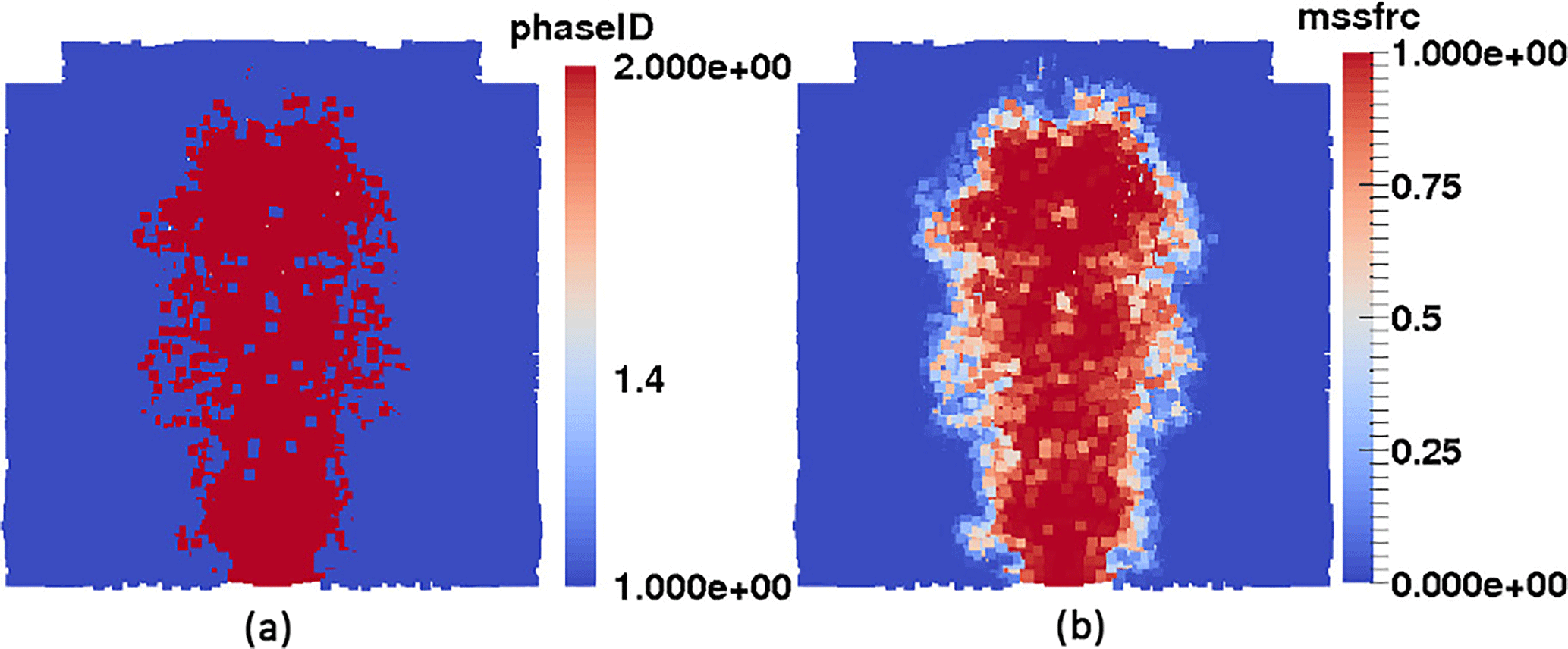
In areas far away from the interface, updating of density is exactly the same as that for single-phase flow. For example, on the right side and left side (or blue areas) in Fig. 1, where there are only air particles, Eq. (59) evaluates to zero, and total density is
which is a special case of Eq. (56). For these areas occupied by only particles of phase 2 and far away from the interface, similarly, the equation for the density update becomes
That is to say, the same density updating equation can be applied for both phases and no additional numerical treatment is needed to locate where the interface is.
Interface construction will become necessary and important when attempting to include the effects of mixing by resolving the detailed interface structure and dynamics of turbulence. As a Lagrangian method, interface tracking in SPH is explicit through capturing of the locations of the particles, much simpler than Eulerian methods. The existence of complex evolving interfaces between phases presents severe challenges to conventional Eulerian grid-based numerical methods. Either interface tracking (Lagrangian) (Harlow and Welch, 1965; Wrobel and Brebbia, 1991; Cheng and Armfield, 1995) or interface capturing (Eulerian) (Hirt and Nichols, 1981; Youngs, 1982; Gerlach et al., 2006; Gopala and van Wachem, 2008) methods are used to reconstruct the flow interface of free boundary flow. High computational cost, a tendency to form numerical instabilities and the inability to track complex topological changes are the significant drawbacks of tracking techniques (Hirt and Nichols, 1981; Unverdi and Tryggvason, 1992; Anderson et al., 1998). For the interface capturing (Eulerian) method, the surrendering of surface detail before the phase transport calculation means that interface reconstruction is required between time steps to recover the interface information, which needs additional numerical effort (Hirt and Nichols, 1981; Youngs, 1982). Since SPH is able to adaptively adjust the discretization and automatically construct the interface, SPH requires less additional numerical effort for interface construction and therefore is more suitable for volcanic plume simulation.
3.7 Turbulence modeling with SPH
For high-speed shearing flow, the momentum exchange and heat transfer are dominated by turbulent fluctuations as turbulent exchange coefficients are several magnitudes larger than corresponding physical coefficients (molecular viscosity and heat conduction coefficient). In addition to momentum and energy exchange, mixing between plume and air is important in plume modeling. Quantifying these mixing processes in real implementation is challenging because of the scale disparity between the large-scale fluid motion and the diffusion processes on interface that ultimately lead to mixing. Ideally, one would like to be able to include the effects of mixing on the large-scale dynamics without resolving the detailed interface structure and dynamics of turbulence to reduce computational cost. To resolve all turbulent exchange at all different scales and sub-particle-scale mixing with relative coarse resolution, a SPH sub-particle-scale (SPH-SPS) turbulence models should be included. Among existing SPH-SPS turbulence models (Holm, 1999; Monaghan, 2002; Violeau and Issa, 2007; Monaghan, 2011), we adopt a LANS-type turbulence model, the SPH−ε turbulence model (Monaghan, 2011). However, the SPH−ε turbulence model was proposed only for incompressible flow. In the following section, we will extend it for compressible flow. It is necessary to mention that all other existing SPH-SPS turbulence models (Holm, 1999; Monaghan, 2002; Violeau and Issa, 2007) also only focus on incompressible flow.
3.7.1 Lagrangian average in SPH−ε
Monaghan (2011) constructed SPH−ε turbulence model within the framework of SPH in such a way that general principles such as conservation of energy, momentum and circulation are satisfied using the ideas associated with the LANS turbulence modeling. The basic idea of SPH−ε is to determine a smoothed (averaged in space) velocity by a linear operation on the unsmoothed velocity v. The SPH particles move with this smoothed velocity, and hence the average motion of the fluid is determined by the averaged velocity :
The average of physical quantities over space introduces extra terms into the governing equations. Once the form of the smoothing (average) is chosen, these extra terms are determined. The typical LANS model uses a smoothed velocity defined in terms of the unsmoothed velocity v by
where G satisfies
and is a member of a sequence of functions which tends to the δ function in the limit when l→0. A typical example is Gaussian. The length scale l determines the characteristic width of the kernel and the distance over which the velocity is smoothed.
It is a common practice in LANS to use a differential equation for the smoothing rather than the integral form and finally reach a system of equations that need to be solved implicitly. In the SPH−ε method, a XSPH (Monaghan, 1989) smoothing is adopted which conserves linear and angular momentum. In this way, solving a system of equations is avoided, and it also makes the method simple to implement and cheap for computation. The discretized form of the momentum equation is obtained through lengthy derivation. Derivation and other discussions are available in the literature; see, e.g., Monaghan (2011). Here, we provide a brief summary of the key steps.
The smoothing adopted by Monaghan (2011) is
As function G has the same feature as kernel function w, SPH approximation of the integration leads to
By making the replacement,
where Kab=ldGab, M=ρ0ld in which ρ0 is initial density. The SPH−ε turbulence model is obtained after lengthy derivation:
Notice that, if l is constant,
The discretized momentum equation with the SPH−ε turbulence model can be written in terms of Gab instead of Kab:
where
which is the extra stress term induced by average. We take coefficient ε as 0.8 following Monaghan (2011).
For compressible flow, the energy equation is coupled with the momentum equation and mass conservation equation. Averaging of thermal energy over space introduces some additional terms besides the stress term induced by velocity average (Rumsey, 2014). The averaged momentum equation for compressible flow is in the same form as that for incompressible flow; all of the other additional terms, besides the corresponding velocity-average-induced stress term, show up in the energy equation. Most turbulence modeling focuses on the stress terms induced by the average of velocity. These stress terms are usually either solved directly (for example, LANS methods) or defined via a constitutive relation (for example, large eddy simulation method). Less attention is typically given to the other terms. Most commonly, a Reynolds analogy is used to model the turbulent exchange. Simulations of heat transfer, or other scalar transfer, in turbulent flow simply involve adding transport terms for thermal energy or species concentration, at the expense of greater storage and longer computing times but without other difficulties (Cebeci, 2013). We adopt this strategy. The additional terms associated with molecular diffusion and turbulent transport in the energy equation are either modeled in different ways or neglected sometimes (Rumsey, 2014). We neglect these terms in our simulation.
3.7.2 Turbulent heat transfer
We adopt the Reynolds analogy to get the heat transfer coefficient due to turbulence. The Prandtl number is defined as
where μ is the dynamic viscosity, and κ is the thermal conductivity. In addition, μ can be written in terms of the absolute viscosity (kinematic viscosity) as
Then,
The typical value of Prt for air is 0.7–0.9. We take Prt=0.85 for gases as recommended Kays (1994) from summarizing experimental results.
Monaghan (2005) summarized the simulation of viscosity and heat conduction in his review on SPH. We will refer to his summary in our following discussion. The additional term in the discretized momentum equation, Eq. (71), is the turbulent shear stress term. Recall that molecular viscosity can be discretized with SPH as shown in Eq. (38). It has been shown that the discretized molecular viscosity has both bulk viscosity and shear viscosity, where shear viscosity coefficient is (Monaghan, 2005)
with
The turbulent viscosity coefficient can be inferred from that formulation if we can reformulate the turbulent shear stress term in a form which is similar to the molecular shear term. Reformulating the turbulent shear stress term,
the turbulent viscosity coefficient can be inferred from Eq. (78).
Please note that the turbulent viscosity term has the opposite sign of the molecular viscosity term in the discretized momentum equation and there is a minus sign in the expression of Πab, and they cancel out.
However, the above equation is correct only for the 1-D situations. For 2-D or 3-D, it is not easy to get an explicit expression. We adopt an alternative way: obtaining a value for each pair of particles instead of persisting on getting an analytical expression. Choosing the smoothing function to be the same as the SPH kernel and the smoothing length scale l to be the same as the smoothing length h, the ratio between turbulent shear stress and physical shear stress is
Υab is essentially equivalent to the ratio between the turbulent viscous effect of particle b on particle a and molecular viscous effect of particle b on particle a. Turbulent viscosity can be easily obtained by
The corresponding turbulent thermal conductivity should be
and are simply the arithmetic means of specific heat and density. The term used to prevent singularity now can be removed.
We also need to prevent singularity, so
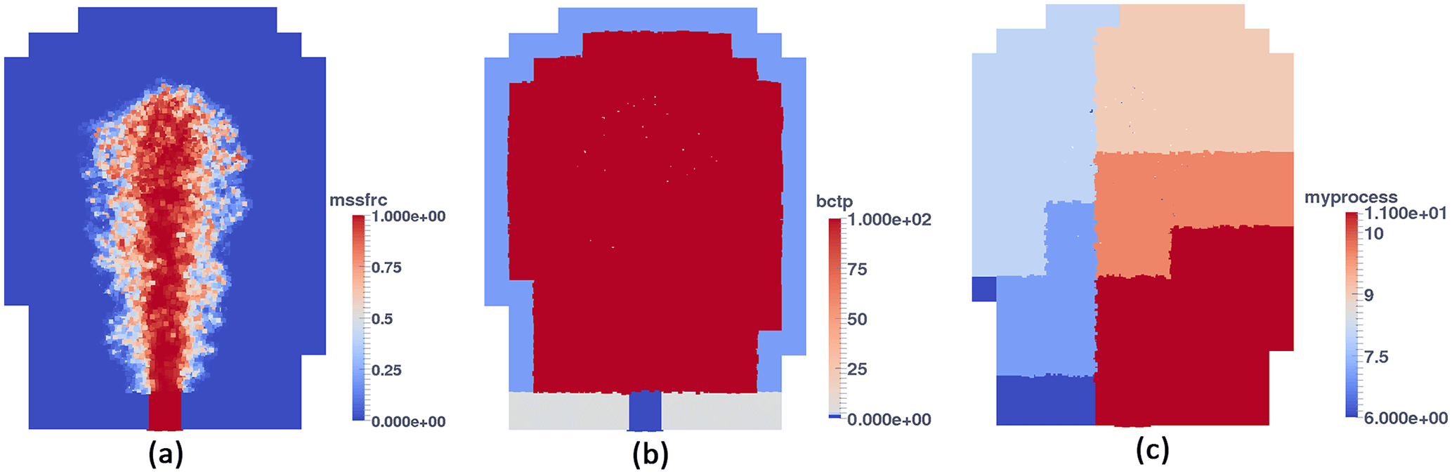
Figure 2A cross-section view of the simulation domain in the y−z plane at 66 s. Panel (a) shows the mass fraction. Panel (b) shows all boundary conditions: the dark blue region is occupied by eruption ghost particles with a “ghost particle ID” of 0; the light blue area is occupied by pressure ghost particles with a “ghost particle ID” of 1; the gray area is filled with wall ghost particles with a “ghost particle ID” of 2. The “ghost particle ID” of all real particles is set to 100; they occupy the major portion of the domain in panel (b). Panel (c) shows the cross-section view of domain decomposition based on SFC. The simulation is conducted on 12 processors, so there are 12 subdomains in total. The cross-section view shows a portion of them.
The heat conduction equation without the source term is
The second spatial derivative can be approximated with SPH by following Monaghan (2005):
where Fab(h) is short for , whose definition is
Fab is always non-positive, which guarantees that heat flux flows from hot to cold. Plug the turbulent thermal conductivity into the heat conduction equation:
Notice that the number “2” in the front of Eq. (88) comes from integration approximation of the second-order derivative (Cleary and Monaghan, 1999). By further simplification, we get
3.7.3 Discretized governing equations with SPH−ε turbulence model
Plugging in the discretized turbulent stress term and turbulent heat transfer term into the momentum and energy equation, we get new discretized governing equations:
with
with κt,αβ given by Eq. (84). As the particle-scale movement of flow is based on smoothed velocity, the velocity in the energy equation should also be smoothed. The filtering process is done according to Eq. (67). Position of particles is updated according to Eq. (63). Smoothed velocity is also used while computing artificial viscosity.
3.8 Boundary conditions
All boundary conditions are imposed by ghost particles. Figure 2b shows how boundaries are deployed.
3.8.1 Wall boundary condition
Traditionally, either ghost particles that mirror real particles across the boundary (Ferrari et al., 2009) or boundary forces (Monaghan and Kajtar, 2009) have been used to impose the wall boundary conditions. One disadvantage of the latter is that the boundary forces tend to corrupt the solution in the local neighborhood. In addition, a natural way of imposing the eruption boundary condition is using eruption ghost particles. To impose boundary conditions in a consistent way, we adopt a modified version of the ghost particle method (Kumar et al., 2013) for wall boundary conditions. Stationary wall ghost particles are deployed in the same way as real particles. Instead of enforcing symmetry particle by particle, a symmetric field across the boundary is explicitly enforced. Ghost particles are reflected into the domain and physical quantities are calculated at these reflected positions by SPH interpolations. It should be noted that wall ghost particles should not be counted when computing physical properties of these reflected positions. All properties, except for velocity, are assigned at the corresponding reflected position to the ghost particle. The velocity of each wall ghost particle is set to have the same value but opposite direction of the interpolated velocity at its corresponding reflection. This way, the non-slip wall boundary condition (Eq. 22) is imposed naturally. These wall ghost particles serve as neighbors in momentum and energy update. More implementation details about this method can be found in Kumar et al. (2013). As these wall ghost particles are stationary, there is no mass flux on the boundary (Eqs. 20 and 21). In addition, as temperature is also symmetric with respect to the boundary, the gradient of temperature vanishes, and hence there is no internal energy flux on the wall boundary (Eq. 23). In our current model, the ground is assumed to be flat. For more complicated topography, it has been shown in other work (Kumar et al., 2013) that this method works as well. We do have concern regarding potential limitation of this method of deployment of ghost particles for more complicated boundaries in three dimensions. Fortunately, the current model does not involve complicated wall boundary.
3.8.2 Eruption boundary condition
A natural way of imposing eruption boundary condition is using ghost particles that move with the eruption velocity and bear the temperature of the erupted material. A parabolic velocity profile that represents a fully developed Hagen–Poiseuille flow is used to determine the inlet particle velocity. The detailed shape of the parabolic profile is determined based on an averaged eruption velocity (Eq. 18). The mass of eruption ghost particles is set to a value so that evaluation of Eq. (46) can return a density that is consistent with the value given in Eq. (16). The internal energy associated with these particles is set to a value so that Eq. (19) is satisfied. The mass fraction of erupted material (Eq. 17) is automatically satisfied as all particles in the eruption conduit are of phase 2. The density, momentum and internal energy of these eruption ghost particles are not updated before they move aboveground. As soon as they move out from eruption conduit, these ghost particles will be shifted to real particles and their physical quantities and position will be updated based on discretized governing equations. New ghost particles need to be added at the bottom of the eruption conduit as these existing ghost particles move upwards.
3.8.3 Pressure boundary condition
Another boundary condition in our model is the pressure outlet boundary. For flow in a straight channel, it is possible to treat the exit the same as the entry with a prescribed velocity profile. For flow with a more complex channel, an exit far downstream of the flow disturbance is also feasible. However, the natural boundary condition (Eq. 24) is more suitable for plume simulation as the outlet is open atmosphere. The way we impose pressure boundary condition is by adding several layers of pressure ghost particles surrounding the real atmosphere particles. Pressure, density and temperature are determined based on the elevation of particles. Velocity is set to zero for static atmosphere. The physical quantities for pressure ghost particles are not updated while these for real particles are updated at every time step. As the position of all pressure ghost particles keeps constant, we essentially impose a static pressure boundary condition. Real particles are removed as soon as they move out of the pressure boundary.
As simulations progress, changes in position and physical quantities of real particles near pressure boundaries might corrupt the pressure boundary condition that was established initially. This shortcoming is relieved by choosing a larger computational domain so that boundaries that might be corrupted are far away from turbulent mixing area. In addition, to avoid enlarging fluctuations, we add another constraint on the time step:
where CFLp is a safety coefficient which has similar function to the normal Courant–Friedrichs–Lewy (CFL) number. Too small CFLp would slow down simulation, while too large CFLp would lose its ability of mitigate numerical fluctuation near the boundary. The proper CFLp is determined by a series of simulation tests.
3.9 Parallelism and performance
One disadvantage of the 3-D model is that it usually takes a much longer time than 1-D models to complete one simulation. This disadvantage further prevents simulation with finer resolution and accounting for more physics in one model. Non-intrusive uncertainty analysis, which is commonly adopted in hazard forecasting, requires finishing multiple simulations within a given time window. High-performance computing is therefore essential. Among existing CPU parallel SPH schemes, most of them focus on the neighbor search algorithm and dynamic load balancing (Ferrari et al., 2009; Crespo et al., 2015). Less attention has been paid to developing more flexible data management schemes for more complicated problems. Motivated by techniques developed for mesh-based methods, we develop a complete framework for parallelizing SPH with distributed memory parallelism (MPI) allowing flexible and efficient data access.
The time complexity for an SPH method is O(N2), where N is the total number of SPH particles. Efficient neighbor searches and compact-supported kernel functions can help to reduce computational cost. Of the many possible choices, we adopt a background grid which was proposed by Monaghan and Lattanzio (1985) and is quite popular in parallel SPH. Then, the time complexity is reduced to O(MN+mN), where m is the average of number of particles within the compact support of the kernel function, M is the average number of particles in subdomain within which neighbor searches are carried out. This background grid is also used for domain decomposition. We refer to the elements of the background grid, namely squares for two dimensions and cubes for three dimensions, as buckets. As for the actual storage of the physical quantities, different strategies have been adopted in existing implementations of SPH.
In DualSPHysics (Crespo et al., 2015), the physical quantities of each particle (position, velocity, density, etc.) are stored in arrays. The particles (and the arrays with particle data) are reordered following the order of the cells. This has two advantages: (1) the access pattern is more regular and more efficient; (2) it is easy to identify the particles that belong to a cell by using a range since the first particle of each cell is known. But adding, deleting and especially accessing particles are cumbersome. Ferrari et al. (2009) adopted linked lists using pointers so that particles can be deleted or added during the simulation. Storage problems caused by fixed-size arrays are thereby also eliminated. We define C++ classes which contain all data of particles and buckets. As for the management of data, we adopt hash tables to store pointers to particles and buckets, which gives us not only flexibility of deleting and adding elements but also quicker access compared with linked lists. Instead of using the “natural order” to number particles, we adopt a SFC-based index to give each particle and background bucket a unique identifier – a strategy known to preserve data locality at minimal cost. The SFC-based numbering strategy is further extended to include time step information so that particles added at the same position but different time have different identifiers.
The parallelization is achieved by splitting computational domain into subdomains. Each subdomain is computed by a single processor. For any subdomain, information from its neighboring subdomains is required when updating physical quantities. To guarantee consistency, data are synchronized if physical quantities are updated. Even though more complicated graph-based partitioning tools (Biswas and Oliker, 1999) might get higher quality decomposition, they require much more effort in programming and computation. So we adopt an easy programming scheme based on SFC (Patra and Kim, 1999) to decompose the computational domain. Figure 2c shows a cross-section view of domain decomposition.
More details about the data structure, domain decomposition, load balancing, domain adjusting and performance benchmarking have been published separately (Cao et al., 2017).
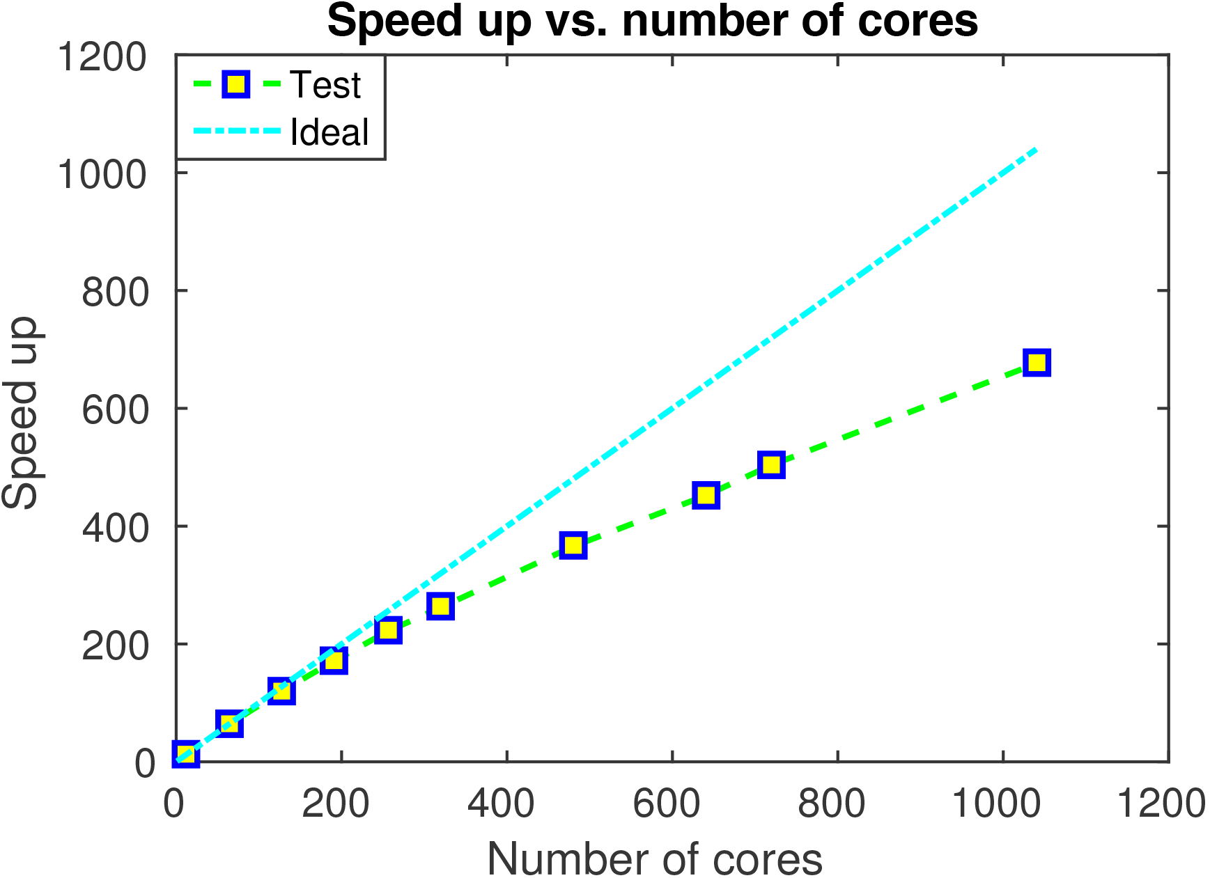

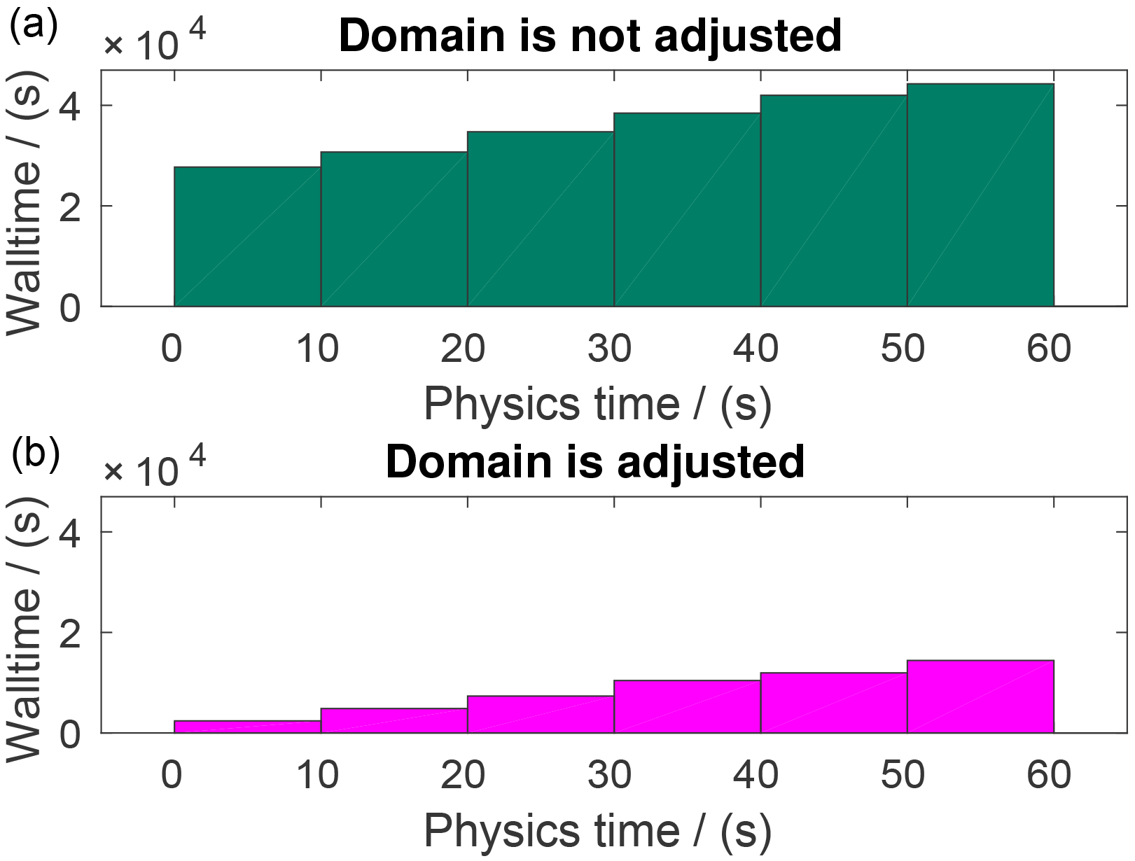
Figure 5The effect of domain adjusting on simulation time. Panel (a) shows execution time without domain adjusting; panel (b) shows execution time with domain adjusting. Different bins represent execution time up to specific physical time indicated by horizontal axis.
Performance tests have been carried out on the computational cluster of Center for Computational Research (CCR) at the University at Buffalo. Intel Xeon E5645 CPUs running at 2.40 GHz clock rate with 4 GB memory per core on a Q-Logic Infiniband are used in these tests. Each node is comprised of two sockets with six of these cores. Memory and level 3 cache are shared on each node. The initial domain is [−4.8 km, 4.8 km] × [−4.8 km, 4.8 km] × [0 km, 6 km]. Almost linear speed up is observed in our strong scalability test (Fig. 3).
The weak scalability test is conducted with the same initial domain and various smoothing lengths. Each simulation runs for 400 time steps. The average number of real particles of each process keeps constant at 25 900. As shown in Fig. 4, simulation times increase around one-third when the number of cores increases from 16 to 4208. For the test problem in this section, the volcanic plume finally reaches a region of [−30 km, 30 km] × [−30 km, 30 km] × [1.5 km, 40 km] after around 400 s of eruption. When numerical simulation goes up to 90 s, the plume is still within a region of [−10 km, 10 km] × [−10 km, 10 km] × [0 km, 25 km]. This implies that adjusting of domain can avoid computing a large number of uninfluenced air particles, especially for the beginning stage of simulation. A domain-adjusting algorithm (Cao et al., 2017) is designed and implemented in our code. Figure 5 shows that simulation time of the test problem is greatly reduced when we adopt the domain-adjusting strategy.
We present a series of numerical simulations to verify and validate our model in this section. Plume-SPH is first verified by 1-D shock tube tests, then by a JPUE (jet or plume that is ejected from a nozzle into a uniform environment) simulation. Velocity and mass fraction distribution both along the central axis and cross transverse are compared with experimental results. The pattern of ambient particle entrainment is also clearly shown. Then, a simulation of representative strong volcanic plume is conducted. Integrated local variable are comparable with simulation results from existing 3-D plume models.
4.1 1-D shock tube tests
1-D shock tube tests are first conducted to verify our code. Input parameter of each tests can be found in Table 1. These tests can represent typical cases in 1-D. Test 1 consists of a left rarefaction, a right traveling contact and a right shock. Density decreases downwind of the contact wave. Test 2 also consists of a left rarefaction, a right traveling contact and a right shock. Density increases downwind of the contact wave. Test 3 is a double expansion test with different initial density.
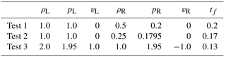
In Table 1, subscript “L” refers to the left side and “R” to the right side; tf is the total simulation time. The initial interval between two adjacent particles is 0.03. The computational domain is . The specific internal energy is compared against exact solutions. As shown in Fig. 6, the position and magnitude of the waves are correctly predicted. The fluctuations near the contact discontinuity are caused by sharp change of smoothing length.
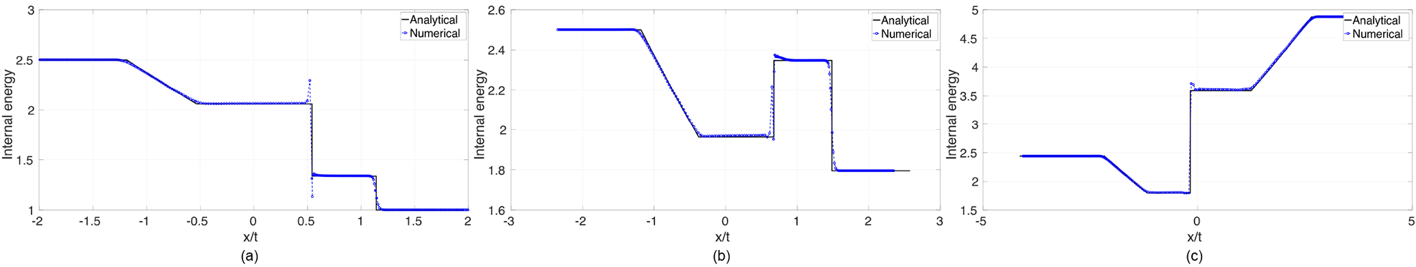
Figure 6Comparison of specific internal energy of simulation results against analytical results for shock tube tests. The plots from left to right correspond to test 1, test 2 and test 3, respectively.
4.2 Simulation of JPUE
JPUE can be considered as a simplified volcanic plume. While the effect of stratified atmosphere and the effect of expansion due to high temperature in volcanic plume are not represented, JPUE reproduces the entrainment due to turbulent mixing which is one of the key elements in the volcanic plume development. There exist consistently good experimental data (List, 1982; Dimotakis et al., 1983; Papanicolaou and List, 1988; Ezzamel et al., 2015) that describe the JPUE flow field giving insight into details of JPUE, such as transverse velocity and concentration profile. In this section, we verify that our code and the SPH−ε turbulence model is able to reproduce the features of turbulent entrainment by a JPUE simulation.
As many of these experiments were conducted with liquid, we replace the original equation of state (Eq. 5) with a weakly compressible Tait equation of state (Becker and Teschner, 2007) (see Eq. 94) to avoid solving the Poisson equation:
with γ=7 and B is evaluated by
where c is the speed of sound in the liquid. The energy equation is actually decoupled from the momentum conservation equation and the mass conservation equation by using this EOS. In addition, the “atmosphere” is assumed to be uniform and gravity is set to be zero. We set the temperature and density of ejected material the same as surrounding ambient. This further simplifies the scenario for the convenience of studying turbulent mixing.
One overall feature of JPUE is “self-similarity”, which means that the evolution of the JPUE is determined solely by the local scale of length and velocity, which theoretically account for the fact that the rate of entrainment at the edge of JPUE is proportional to a characteristic velocity at each height. As a result, physical and numerical experiments do not necessarily have exactly the same setups and are compared on a non-dimensional basis.
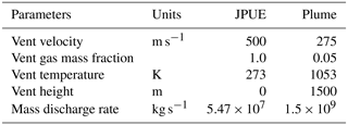
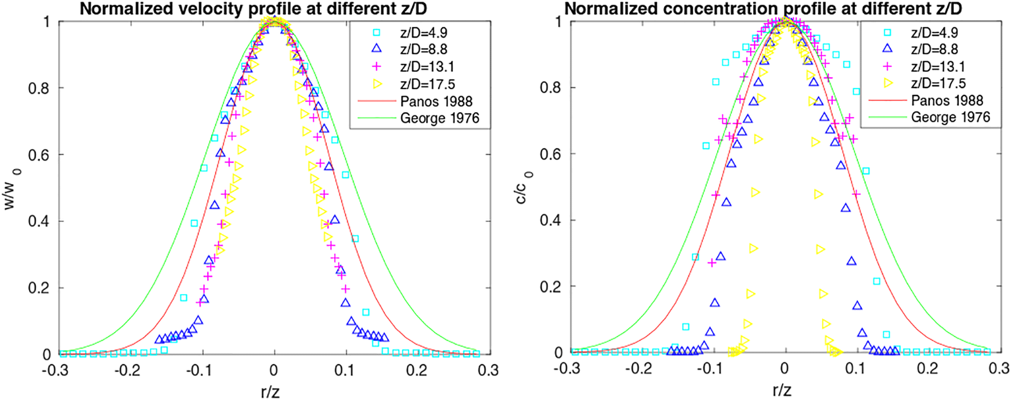
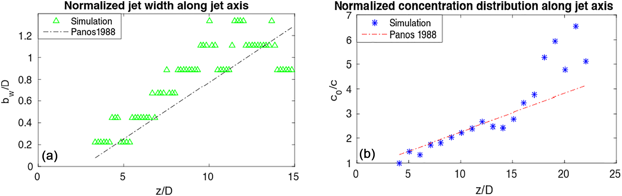
Figure 8Panel (a) shows normalized jet width (which determined based on velocity) along the centerline. Panel (b) shows normalized concentration along the centerline.
A three-dimensional axisymmetric JPUE which ejects from a round vent is simulated with eruption parameters listed in Table 2. Material properties of water are used as material properties for both phases. The results are compared with experiments (George et al., 1977; Papanicolaou and List, 1988) for verification purposes. Experimental data of concentration and velocity distribution across the cross section were fit into a Gaussian profile (see Eq. 96) by Papanicolaou and List (1988) and George et al. (1977) even though the actual profiles are slightly different from the Gaussian profile.
where φ is either velocity or concentration, the subscript “c” represents the centerline. r is the distance from the centerline on any cross section. z is the axial distance from the origin of the jet transverse section under consideration. The coefficient “coef” for concentration is 80 and 50, respectively, according to George et al. (1977) and Papanicolaou and List (1988). The “coef” for velocity is 90 and 55, respectively, according to George et al. (1977) and Papanicolaou and List (1988).
Papanicolaou and List (1988) also fit concentration distribution and jet width based on velocity along the centerline into a straight line (see Eq. 97).
where subscript 0 represents the cross-sectionally averaged exit value; D is the diameter of vent. The “slope” for jet width based on velocity is 0.104 and for concentration is 0.157. The “intercept” for jet width based on velocity is 2.58, while that for the concentration is 4.35.
Although both velocity and concentration are found to be well matched with experimental results, a small disparity in both velocity and concentration is observed near the boundary of the jet, which is possibly caused by overestimation of the drag effect by standard SPH (Ritchie and Thomas, 2001). Ritchie and Thomas (2001) also proposed an alternative way to update density which relieved the overestimating of the drag effect. However, how well this method conserves mass is not clear. There are several other factors that might also attribute to such disparity. The Reynolds number is not reported in many experiments assuming a high enough Reynolds number. In addition, some details of the experiments, such as exit velocity profile and viscosity of the experimental liquid, are not reported. These factors prevent us from numerically reproducing these experiments in an exact way as they were conducted. However, the features of JPUE are correctly reproduced with our code.
We also investigated the mixing due to turbulence in the JPUE simulation by checking the mixture of the two phases. It is shown in Fig. 9 that the ejected material and ambient fluids are mixed through eddies at the outer shear region. Also, the inner dense core dispersed gradually due to erosion of the outer shear region. Hence, our confidence in the numerical correctness of our code is greatly reinforced.

Figure 9Panel (a) shows particle distribution. Particles of phase 1 (blue) are gradually entrained and mixed with erupted particles (red) as jet flows downstream. Panel (b) shows the mass fraction of erupted material at the moment corresponding to panel (a).
4.3 Simulation of a volcanic plume
The development of a volcanic plume is more complicated than JPUE in several aspects. Besides turbulent entrainment of ambient fluids, development of the volcanic plume also involves heating of entrained air and expansion in a stratified atmosphere. A strong eruption column without wind is tested in this section for the purpose of further verification and validation. Both global variables and local variables are compared with existing models.
4.3.1 Input parameters
Eruption parameters, material properties and atmosphere are chosen to be the same as the strong plume no-wind case in a comparison study on eruptive column models by Costa et al. (2016). Eruption conditions are listed in Table 2. As our model does not distinguish solid particles of different sizes, only mass fraction of solids of all sizes is used in simulation even though two size classes were provided by Costa et al. (2016). The density of erupted material at the vent and radius of the vent can be computed from the given parameters. The eruption pressure is assumed to be the same as the ambient pressure at the vent and hence is not given in the table. The vertical profiles of atmospheric properties were obtained based on the reanalysis data from the European Centre for Medium-Range Weather Forecasts (ECMWF) for the period corresponding to the climactic phase of the Mt. Pinatubo eruption (Philippines, 15 June 1991). These conditions are more typical of a tropical atmosphere (see Fig. 1b in Costa et al., 2016). Vertical distribution of temperature, pressure and density is used to establish stratified atmosphere. Wind velocity and specific humidity are not used in our simulation even though they were also provided by Costa et al. (2016) (see Fig. 1b). Material properties, shown in Table 3, are selected based on properties of the Pinatubo and Shinmoedake eruptions. Other material properties not given in the table can be inferred from these given parameters based on their relationships.
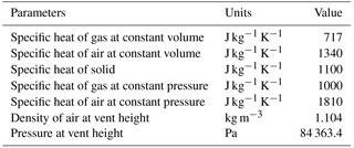
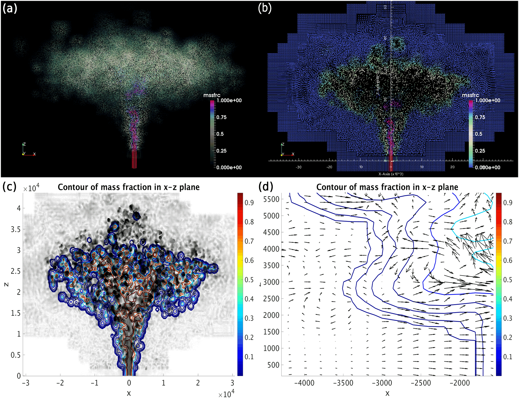
Figure 10Mass fraction for t=500 s after eruption. Panels (a, b) are visualizations of SPH simulation results. Panel (b) shows visualization of a slice of the computational simulation, whose thickness is around 10 000 m. The lowest portion of the plume represents erupted material in the eruption vent (the underground portion). Panels (c, d) show the contour of the mass fraction and velocity quiver on an x−z plane. These panels are plotted utilizing postprocessed data (see Appendix A). The contour levels in the plot are 0.00001, 0.0001, 0.001, 0.1, 0.3, 0.75 and 0.95. Panel (d) is a zoomed view of velocity quiver showing plume expansion and entrainment of air.
Figure 10 shows the mass fraction of the simulated volcanic plume at 500 s after eruption, at which time the plume starts spreading radially. A contour plot of the mass fraction on the vertical cross section (x−z plane) was also provided. The zoomed view of the quiver plot shows detailed entrainment of air at the margin of the plume.
4.3.2 Global and local variables
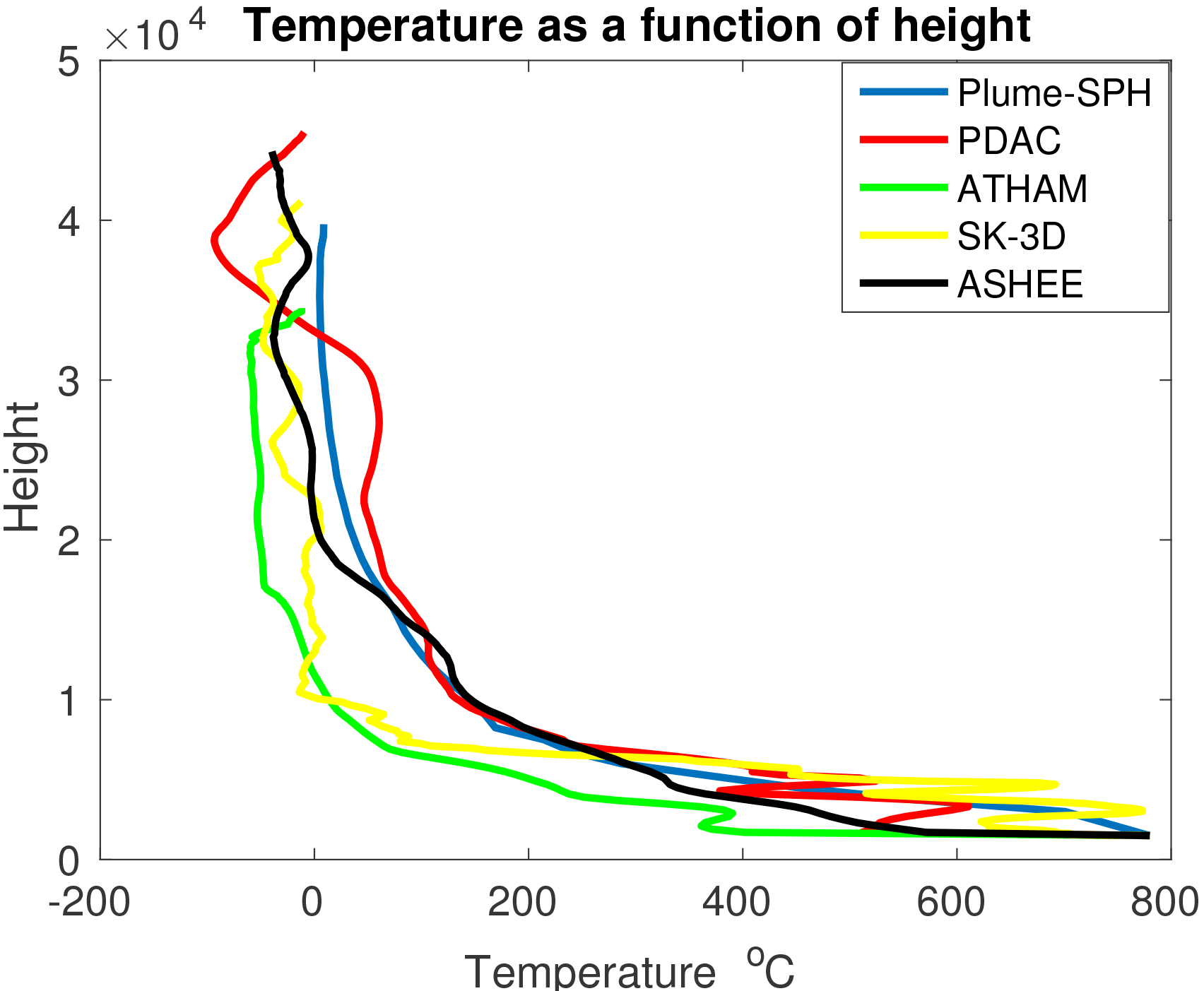
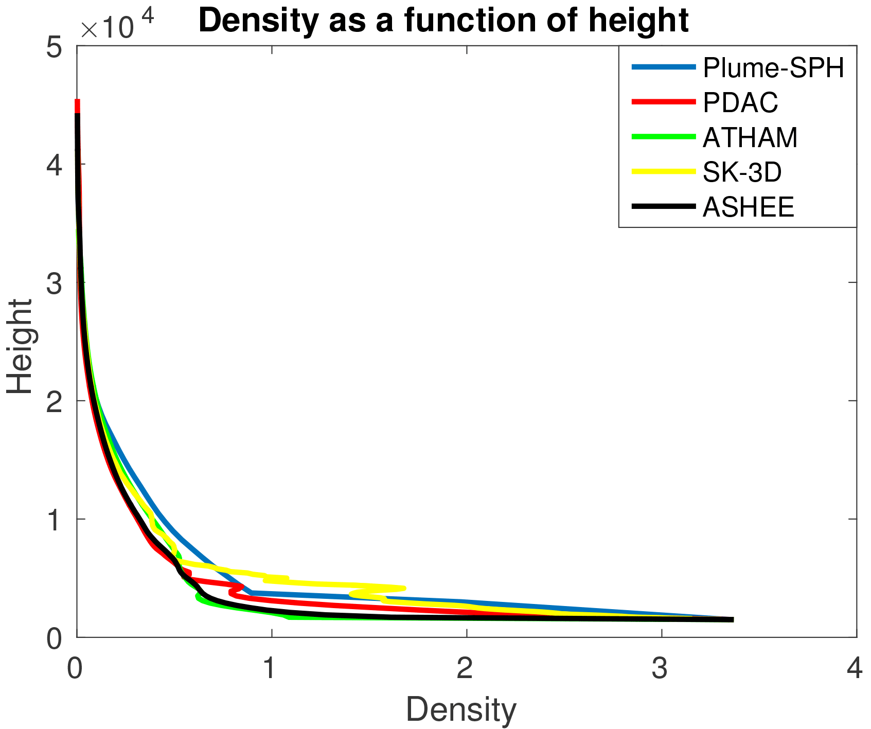
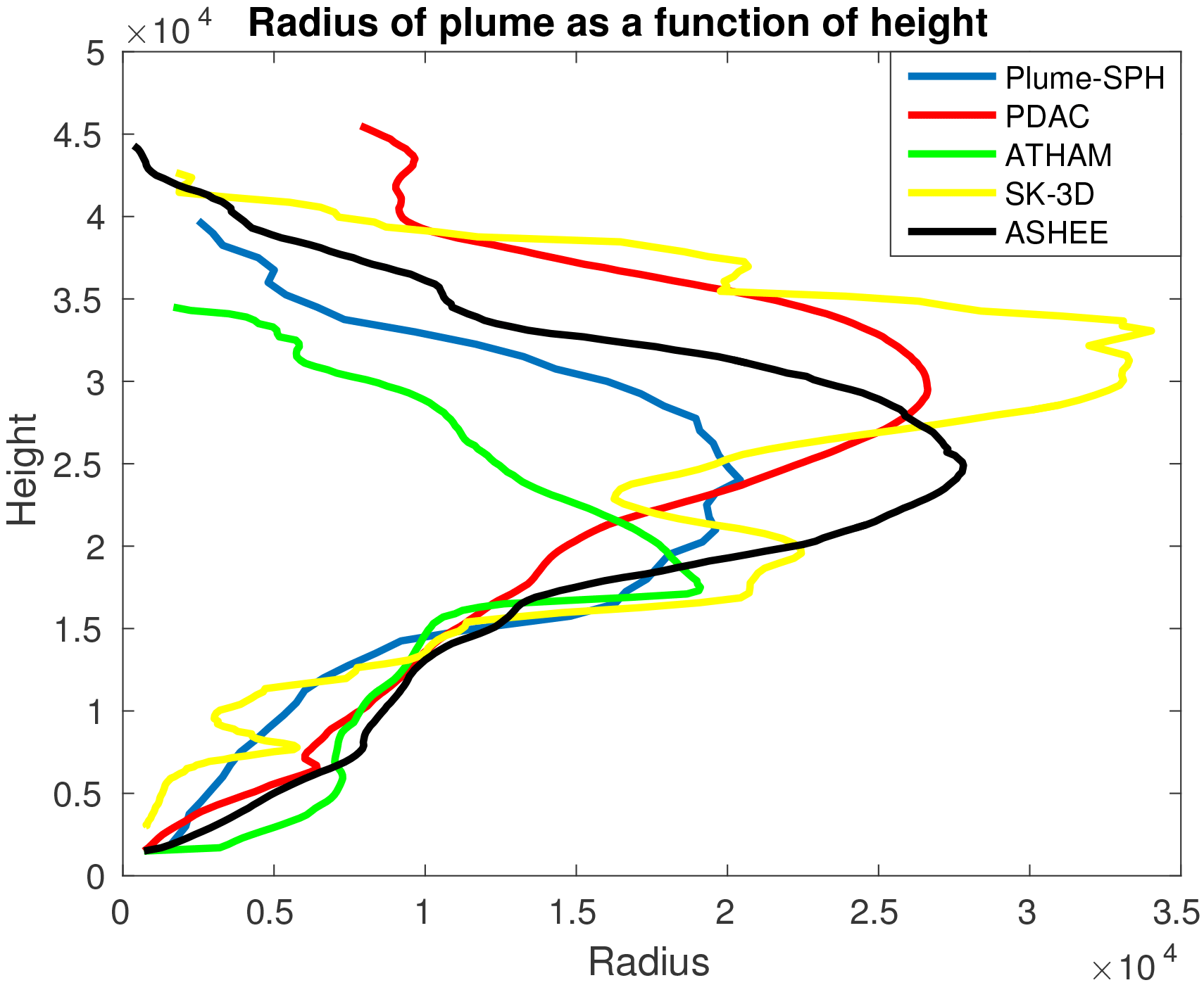
One of the key global quantities of great interest is the altitude to which the plume rises. The top height predicted by our model is around 40 km which agrees with other plume models. For example, the height predicted by PDAC is 42 500 m, by SK-3D is 39 920 m, by ATHAM is 33 392 m and by ASHEE is 36 700 m. As for local variables, the profiles of integrated temperature, density, mass fraction of entrained air, gas mass fraction, mass fraction of solid materials and the radius of the plume as a function of height are compared with existing 3-D models in Figs. 11–14. To get rid of significant fluctuations in time and space, we conducted a time-averaging and spatial integration of the dynamic 3-D flow fields by following Cerminara et al. (2016b).

As particles distribute irregularly in the space in SPH simulation results, we need to project simulation results (on irregular particles) onto a predefined grid before doing time-average and spatial integration. See Appendix A for more details of postprocessing.
The profiles of local variables match well with simulation results of existing 3-D models in a general sense. The basic phenomena in volcanic plume development are correctly captured by our model.
As the height increases, the amount of entrained air also increases. Around the neutral height, where the umbrella expands, the entrainment of air shows a slight decrease due to lack of air surrounding the column at that height. The profile for gas, which accounts for both air and vapor, shows a very similar tendency to that of entrained air. Recall that vapor condensation is not considered in our model. In addition, we assume that erupted material behaves like a single-phase fluid. So the mass fraction of gas is simply a function of entrained air (Eq. 98).
Among these 3-D models, ATHAM takes vapor condensation into account and Eq. (98) does not hold for ATHAM. However, the profile of entrained air and profile of gas predicted by ATHAM are still very close to each other, which implies that ignoring water phase change is a valid assumption for eruptions similar to this test case (strong plume with erupted water fraction in erupted material less than 5 %). This observation can be explained by the fact that air occupies a larger portion of the gas, and ignoring phase change of vapor (which is only a small portion of gas) has a slight influence on plume development. As for mass fraction of solids, similarly, Eqs. (99) and (100) hold for our model.
PDAC, which treats particles of two different sizes as two separate phases, predicted a similar mass fraction profile. That implies that assumption of dynamic equilibrium in our model is at least valid for eruptions similar to the test case.
With more cool air entrained into the plume and mixing with the hot erupted material, the temperature of the plume decreases as the height increases as shown in Fig. 11. Meanwhile, bulk density decreases due to entrainment and expansion (Fig. 13).
Our model adopts the same assumptions and governing equations as SK-3D. However, there is still an obvious disparity between the profiles of local variables of our model and SK-3D. One of the big differences between these two models is that we adopt a LANS type of turbulence model while SK-3D adopts a large eddy simulation (LES) turbulence model. This implies that choice of turbulence model might play a critical role in plume simulation.
A new plume model was developed based on the SPH method. Extensions necessary for Lagrangian methodology and compressible flow were made in the formulation of the equations of motion and turbulence models. Advanced numerical techniques in SPH were exploited and tailored for this model. High-performance computing was used to mitigate the tradeoff between accuracy (which depends on comprehensiveness of the model, resolution, order of accuracy of numerical methods, scheme for time upgrading) and simulation time (which depends on comprehensiveness of model, resolution, order of accuracy of numerical methods, scheme for time upgrading, etc. and computational techniques). The correctness of the code and model was verified and validated by a series of test simulations. Typical 1-D shock tube problems were simulated and compared against analytical results showing good agreement. Dimensionless velocity and concentration distribution across the cross section and along the jet axis match well with experimental results of JPUE. Top height and integrated local variables simulated by our model are consistent with simulation results of existing 3-D plume models. Comparison of our results with those of SK-3D implies that the turbulence model plays a significant role in plume modeling.
Currently existing 3-D models focus on certain aspects of the volcanic plume (PDAC on pyroclastic flow, ATHAM on microphysics and SK-3D on entrainment with higher resolution and higher order of accuracy), and hence, naturally, different assumptions were made in these models. However, these different aspects of volcanic plumes are not independent but are actually coupled. For example, it has been illustrated by Cerminara et al. (2016b) that gas–particle non-equilibrium would introduce a previously unrecognized jet-dragging effect, which has great influence on plume development, especially for weak plumes. In addition, there is no absolute boundary to determine which kind of hazard is dominant in certain eruptions. So it is necessary to simulate all associated hazards in one model. Actually, effort has already been put into developing more comprehensive plume models. For example, a large-particle module (LPM) was added to ATHAM to track the paths of rocky particles (pyroclastic or tephra) within the plume and predict where these particles fall (Kobs, 2009). We were also motivated by such an evolution of plume modeling to choose SPH as our numerical tool. Besides its ability to deal with interfaces for multiphase flows, as mentioned in the introduction section, the SPH method has good extensibility and adding new physics and phases requires much less modification of the code compared with mesh-based methods. Last but not least, the dramatic development of computational power makes it possible to establish a comprehensive model. While current computational capacity may not allow us to have a fully comprehensive model, the easy-extension feature of SPH makes it convenient to keep adding new physics into the model when necessary and computationally feasible.
We have presented in this paper an initial effort and results towards developing a first principle-based plume model with comprehensive physics, adopting proper numerical tools and high performance computing. More advanced numerical techniques, such as adaptive particle size, Godunov-SPH, semi-explicit time-advancing schemes and better data management strategies and algorithms are on our list to exploit in the future. In the near future, the effect of wind field will be taken into account. Our code will also be made available in the open-source form for the community to enhance. Besides improving the plume model, coupling the volcanic plume model with magma reservoir models (e.g., Terray et al., 2018), which could provide more accurate eruption conditions, might improve accuracy of the volcanic plume simulation.
The Plume-SPH code, together with a user manual providing instructions for installation, running and visualization, is archived at https://zenodo.org/record/572819#.WRCy7xiZORs (https://doi.org/10.5281/zenodo.572819).
The input data for all simulations presented in this work are archived in the same repository. The MIT license governs the distribution and use of the code and associated documentation files. Permission is granted, free of charge, to any person to deal with the software without restriction. The complete copyright statement can be found in the repository: https://github.com/Plume-SPH/plume-sph/blob/master-1.0/COPYING.
User manual and input data for test runs are also archived in the same repository.
Output data of simulations presented in the paper are around tens of gigabytes and are archived in UBbox. Access will be provided to all upon request.
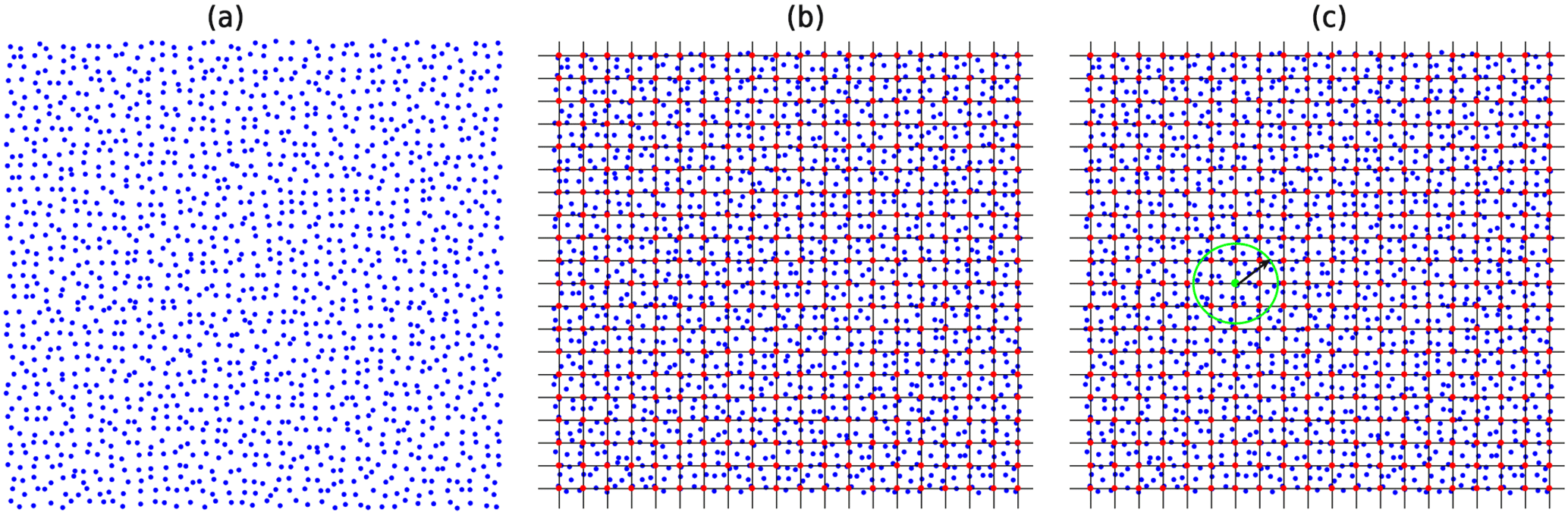
Figure A1Procedure of projection of simulation results carried by particles onto regular grids, as shown in these figures from left to right: (a) raw data of SPH simulation results (irregularly distributed in space), (b) addition of a regular mesh and (c) searching for neighbors of each node (the blue SPH particles within the green circle around the red dot). The last step is not shown in these pictures, which treats each node on the regular mesh as a SPH particle and projects data on particles onto nodes utilizing SPH interpolation (see Eq. 31).
Particles distribute irregularly in SPH simulation results. To adapt postprocessing originally proposed for the mesh-based method, we need to project simulation results onto a predefined regular mesh. As shown in Fig. A1, the basic steps for such projection are to
-
obtain raw simulation results carried by particles that irregularly distribute in the space,
-
create regular grids,
-
search for neighbor particles for each node of the regular grids and
-
interpolate physical quantities from neighbor particles onto the corresponding node of regular grids according to Eq. (31).
ZC was the primary developer of the Plume-SPH code. All co-authors contributed equally to the formulation, analysis and writing of this paper.
The authors declare that they have no conflict of interest.
All developers of Titan-2D, especially Dinesh Kumar who developed the GSPH
version of Titan-2D, are greatly appreciated as Plume-SPH is based on their
code. Advice and data (which are not shown in this paper) given by
Suzuki Yujiro gave us great help at the initial stage of model establishment
and therefore are greatly appreciated. We appreciate Tomaso Esposti Ongaro for
providing simulation data of PDAC (also provided by Antonio Costa later,
together with simulation results of other plume models) which helped us in
early verification and improvement. We appreciate Antonio Costa for
providing simulation results of existing 3-D models, which are used in the
verification and validation section of this paper. We thank Matteo Cerminara
for his help on postprocessing of plume simulation results and his careful
review of our manuscript and constructive remarks. Comments by another
anonymous reviewer are appreciated as well. Computational results reported
here were performed at the Center for Computational Research at the
University at Buffalo. This project is supported by grant no. NSF
ACI/1131074 from the National Science Foundation.
Edited by: Adrian Sandu
Reviewed by: Mattia
de' Michieli Vitturi and
one anonymous referee
Adami, S., Hu, X., and Adams, N.: A new surface-tension formulation for multi-phase SPH using a reproducing divergence approximation, J. Comput. Phys., 229, 5011–5021, 2010. a
Anderson, D., McFadden, G. B., and Wheeler, A.: Diffuse-interface methods in fluid mechanics, Annu. Rev. Fluid Mech., 30, 139–165, 1998. a
Becker, M. and Teschner, M.: Weakly compressible SPH for free surface flows, in: Proceedings of the 2007 ACM SIGGRAPH/Eurographics symposium on Computer animation, Eurographics Association, 209–217, 2007. a
Biswas, R. and Oliker, L.: Experiments with repartitioning and load balancing adaptive meshes, in: Grid Generation and Adaptive Algorithms, Springer, 89–111, 1999. a
Bursik, M.: Effect of wind on the rise height of volcanic plumes, Geophys. Res. Lett., 28, 3621–3624, 2001. a
Bursik, M., Martınez-Hackert, B., Delgado, H., and Gonzalez-Huesca, A.: A smoothed-particle hydrodynamic automaton of landform degradation by overland flow, Geomorphology, 53, 25–44, 2003. a
Bursik, M. I.: bent: A model of plumes in crossflow, available at: https://vhub.org/resources/267 (last access: 15 December 2015), 2010. a
Bursik, M. I., Carbonara, A. U., and Zawicki, S. M.: puffin, available at: https://vhub.org/resources/114 (last access: 15 December 2015), 2013. a
Cao, Z., Patra, A., and Jones, M.: Data Management and Volcano Plume Simulation with Parallel SPH Method and Dynamic Halo Domains, Procedia Comput. Sci., 108, 786–795, 2017. a, b
Carcano, S., Bonaventura, L., Esposti Ongaro, T., and Neri, A.: A semi-implicit, second-order-accurate numerical model for multiphase underexpanded volcanic jets, Geosci. Model Dev., 6, 1905–1924, https://doi.org/10.5194/gmd-6-1905-2013, 2013. a
Carey, S. N. and Sigurdsson, H.: Influence of particle aggregation on deposition of distal tephra from the May 18, 1980, eruption of Mount St. Helens volcano, J. Geophys. Res-Sol. Ea., 87, 7061–7072, 1982. a
Cebeci, T.: Analysis of turbulent flows with computer programs, Butterworth-Heinemann, 27–29, 2013. a
Cerminara, M., Esposti Ongaro, T., and Berselli, L. C.: ASHEE-1.0: a compressible, equilibrium–Eulerian model for volcanic ash plumes, Geosci. Model Dev., 9, 697–730, https://doi.org/10.5194/gmd-9-697-2016, 2016a. a
Cerminara, M., Esposti Ongaro, T., and Neri, A.: Large Eddy Simulation of gas–particle kinematic decoupling and turbulent entrainment in volcanic plumes, J. Volcanol Geoth. Res., 326, 143–171, 2016b. a, b
Chen, J., Beraun, J., and Jih, C.: An improvement for tensile instability in smoothed particle hydrodynamics, Comput. Mech., 23, 279–287, 1999. a, b, c
Chen, Z., Zong, Z., Liu, M., Zou, L., Li, H., and Shu, C.: An SPH model for multiphase flows with complex interfaces and large density differences, J. Comput. Phys., 283, 169–188, 2015. a
Cheng, L. and Armfield, S.: A simplified marker and cell method for unsteady flows on non-staggered grids, Int. J. Numer. Meth. Fl., 21, 15–34, 1995. a
Cleary, P. W. and Monaghan, J. J.: Conduction modelling using smoothed particle hydrodynamics, J. Comput. Phys., 148, 227–264, 1999. a
Colagrossi, A. and Landrini, M.: Numerical simulation of interfacial flows by smoothed particle hydrodynamics, J. Comput. Phys., 191, 448–475, 2003. a
Costa, A., Suzuki, Y., Cerminara, M., Devenish, B., Esposti Ongaro, T., Herzog, M., Van Eaton, A., Denby, L., Bursik, M., de' Michieli Vitturi, M., Engwell, S., Neri, A., Barsotti, S., Folch, A., Macedonio, G., Girault, F., Carazzo, G., Tait, S., Kaminski, E., Mastin, L. G., Woodhouse, M. J., Phillips, J. C., Hogg, A. J., Degruyter, W., and Bonadonna, C.: Results of the eruptive column model inter-comparison study, J. Volcanol Geoth. Res., 326, 2–25, 2016. a, b, c, d, e
Costa, A., Suzuki, Y., and Koyaguchi, T.: Understanding the plume dynamics of explosive super-eruptions, Nat. Commun., 9, 654, https://doi.org/10.1038/s41467-018-02901-0, 2018. a
Crespo, A., Domínguez, J., Rogers, B., Gómez-Gesteira, M., Longshaw, S., Canelas, R., Vacondio, R., Barreiro, A., and García-Feal, O.: DualSPHysics: Open-source parallel CFD solver based on Smoothed Particle Hydrodynamics (SPH), Comput. Phys. Commun., 187, 204–216, 2015. a, b
Degruyter, W. and Bonadonna, C.: Improving on mass flow rate estimates of volcanic eruptions, Geophys. Res. Lett., 39, L16308, https://doi.org/10.1029/2012GL052566, 2012. a
de' Michieli Vitturi, M.: PlumeMoM, available at: https://vhub.org/resources/3541 (last access: 15 December 2016), 2015. a
de' Michieli Vitturi, M., Neri, A., and Barsotti, S.: PLUME-MoM 1.0: A new integral model of volcanic plumes based on the method of moments, Geosci. Model Dev., 8, 2447–2463, https://doi.org/10.5194/gmd-8-2447-2015, 2015. a
Devenish, B.: Using simple plume models to refine the source mass flux of volcanic eruptions according to atmospheric conditions, J. Volcanol Geoth. Res., 256, 118–127, 2013. a
Dimotakis, P. E., Miake-Lye, R. C., and Papantoniou, D. A.: Structure and dynamics of round turbulent jets, Phys. Fluids, 26, 3185–3192, 1983. a
Draxler, R. and Rolph, G.: HYSPLIT (HYbrid Single-Particle Lagrangian Integrated Trajectory) Model access via NOAA ARL READY Website, NOAA Air Resources Laboratory, Silver Spring, available at: https://www.arl.noaa.gov/hysplit/hysplit/, last access: 15 December, 2015. a
Ernst, G. G., Sparks, R. S. J., Carey, S. N., and Bursik, M. I.: Sedimentation from turbulent jets and plumes, J. Geophys. Res-Sol. Ea., 101, 5575–5589, 1996. a
Esposti Ongaro, T., Cavazzoni, C., Erbacci, G., Neri, A., and Salvetti, M.-V.: A parallel multiphase flow code for the 3D simulation of explosive volcanic eruptions, Parallel Comput., 33, 541–560, 2007. a
Ezzamel, A., Salizzoni, P., and Hunt, G. R.: Dynamical variability of axisymmetric buoyant plumes, J. Fluid Mech., 765, 576–611, 2015. a
Ferrari, A., Dumbser, M., Toro, E. F., and Armanini, A.: A new 3D parallel SPH scheme for free surface flows, Comput. Fluids, 38, 1203–1217, 2009. a, b, c
Folch, A., Costa, A., and Macedonio, G.: FPLUME-1.0: An integral volcanic plume model accounting for ash aggregation, Geosci. Model Dev., 9, 431–450, https://doi.org/10.5194/gmd-9-431-2016, 2016. a, b, c
George, W. K., Alpert, R. L., and Tamanini, F.: Turbulence measurements in an axisymmetric buoyant plume, Int. J. Heat Mass Tran., 20, 1145–1154, 1977. a, b, c, d
Gerlach, D., Tomar, G., Biswas, G., and Durst, F.: Comparison of volume-of-fluid methods for surface tension-dominant two-phase flows, Int. J. Heat Mass Tran., 49, 740–754, 2006. a
Gingold, R. A. and Monaghan, J. J.: Smoothed particle hydrodynamics: theory and application to non-spherical stars, Mon. Not. R. Astron. Soc., 181, 375–389, 1977. a
Gopala, V. R. and van Wachem, B. G.: Volume of fluid methods for immiscible-fluid and free-surface flows, Chem. Eng. J., 141, 204–221, 2008. a
Haddad, B., Palacios, D., Pastor, M., and Zamorano, J. J.: Smoothed particle hydrodynamic modeling of volcanic debris flows: Application to Huiloac Gorge lahars (Popocatépetl volcano, Mexico), J. Volcanol Geoth. Res., 324, 73–87, 2016. a
Harlow, F. H. and Welch, J. E.: Numerical calculation of time-dependent viscous incompressible flow of fluid with free surface, Phys. Fluids, 8, 2182, https://doi.org/10.1063/1.1761178, 1965. a
Hérault, A., Bilotta, G., Del Negro, C., Russo, G., and Vicari, A.: SPH modeling of lava flows with GPU implementation, From physics to control through an emergent view, WSS Nonlin. Sci. Ser. B, 15, 183–188, 2010. a
Herzog, M., Graf, H.-F., Textor, C., and Oberhuber, J. M.: The effect of phase changes of water on the development of volcanic plumes, J. Volcanol Geoth. Res., 87, 55–74, 1998. a
Herzog, M., Oberhuber, J. M., and Graf, H.-F.: A prognostic turbulence scheme for the nonhydrostatic plume model ATHAM, J. Atmos. Sci., 60, 2783–2796, 2003. a
Hirt, C. W. and Nichols, B. D.: Volume of fluid (VOF) method for the dynamics of free boundaries, J. Comput. Phys., 39, 201–225, 1981. a, b, c
Holm, D. D.: Fluctuation effects on 3D Lagrangian mean and Eulerian mean fluid motion, Physica D, 133, 215–269, 1999. a, b
Hu, X. and Adams, N. A.: An incompressible multi-phase SPH method, J. Comput. Phys., 227, 264–278, 2007. a
Issa, R.: Numerical assessment of the Smoothed Particle Hydrodynamics gridless method for incompressible flows and its extension to turbulent flows, University of Manchester, 183 pp., 2005. a
Kays, W. M.: Turbulent Prandtl number – where are we?, J. Heat Transf., 116, 284–295, 1994. a
Kobs, S.: Modeling particle motion and near-vent deposition in explosive volcanic eruptions, State University of New York at Buffalo, 2009. a
Koyaguchi, T., Ochiai, K., and Suzuki, Y. J.: The effect of intensity of turbulence in umbrella cloud on tephra dispersion during explosive volcanic eruptions: Experimental and numerical approaches, J. Volcanol Geoth. Res., 186, 68–78, 2009. a
Kumar, D., Patra, A. K., Pitman, E. B., and Chi, H.: Parallel Godunov smoothed particle hydrodynamics (SPH) with improved treatment of Boundary Conditions and an application to granular flows, Comput. Phys. Commun., 184, 2277–2286, 2013. a, b, c
List, E.: Turbulent jets and plumes, Annu. Rev. Fluid Mech., 14, 189–212, 1982. a
Lucy, L. B.: A numerical approach to the testing of the fission hypothesis, Astron. J., 82, 1013–1024, 1977. a
Mastin, L. G.: A user-friendly one-dimensional model for wet volcanic plumes, Geochem. Geophy. Geosy., 8, https://doi.org/10.1029/2006GC001455, 2007. a
Mastin, L. G.: Plumeria 2.3.1, available at: https://vhub.org/resources/1194 (last access: 15 December 2015), 2011. a
Monaghan, J.: On the problem of penetration in particle methods, J. Comput. Phys., 82, 1–15, 1989. a
Monaghan, J.: SPH compressible turbulence, Mon. Not. R. Astron. Soc., 335, 843–852, 2002. a, b
Monaghan, J.: Smoothed particle hydrodynamics, Rep. Prog. Phys., 68, 1703–1759, 2005. a, b, c, d, e, f, g
Monaghan, J.: Smoothed particle hydrodynamics and its diverse applications, Annu. Rev. Fluid Mech., 44, 323–346, 2012. a, b
Monaghan, J. and Gingold, R.: Shock simulation by the particle method SPH, J. Comput. Phys., 52, 374–389, 1983. a
Monaghan, J. and Kocharyan, A.: SPH simulation of multi-phase flow, Comput. Phys. Commun., 87, 225–235, 1995. a
Monaghan, J. and Rafiee, A.: A simple SPH algorithm for multi-fluid flow with high density ratios, Int. J. Numer. Meth. Fl., 71, 537–561, 2013. a
Monaghan, J. J.: Smoothed particle hydrodynamics, Annu. Rev. Astron. Astr., 30, 543–574, 1992. a, b, c
Monaghan, J. J.: A turbulence model for Smoothed Particle Hydrodynamics, Eur. J. Mech. B-Fluid, 30, 360–370, 2011. a, b, c, d, e, f, g
Monaghan, J. J. and Kajtar, J. B.: SPH particle boundary forces for arbitrary boundaries, Comput. Phys. Commun., 180, 1811–1820, 2009. a
Monaghan, J. J. and Lattanzio, J. C.: A refined particle method for astrophysical problems, Astron. Astrophys., 149, 135–143, 1985. a
Neri, A., Esposti Ongaro, T., Macedonio, G., and Gidaspow, D.: Multiparticle simulation of collapsing volcanic columns and pyroclastic flow, J. Geophys. Res-Sol. Ea., 108, 2202, https://doi.org/10.1029/2001JB000508, 2003. a
Oberhuber, J. M., Herzog, M., Graf, H.-F., and Schwanke, K.: Volcanic plume simulation on large scales, J. Volcanol Geoth. Res., 87, 29–53, 1998. a, b
Papanicolaou, P. N. and List, E. J.: Investigations of round vertical turbulent buoyant jets, J. Fluid Mech., 195, 341–391, 1988. a, b, c, d, e, f
Patra, A. and Kim, D.: Efficient mesh partitioning for adaptive hp finite element meshes, in: 11th International Conference on Domain Decomposition Methods, edited by: Lai, C.-H., Bjørstad, P. E., Cross, M., and Widlund, O. B., Domain Decomposition Methods (DDM), 1999. a
Pouget, S., Bursik, M., Singla, P., and Singh, T.: Sensitivity analysis of a one-dimensional model of a volcanic plume with particle fallout and collapse behavior, J. Volcanol Geoth. Res., 326, 43–53, 2016. a
Price, D. J.: Smoothed particle hydrodynamics and magnetohydrodynamics, J. Comput. Phys., 231, 759–794, 2012. a, b
Ritchie, B. W. and Thomas, P. A.: Multiphase smoothed-particle hydrodynamics, Mon. Not. R. Astron. Soc., 323, 743–756, 2001. a, b
Rosswog, S.: Astrophysical smooth particle hydrodynamics, New Astron. Rev., 53, 78–104, 2009. a
Rumsey, C.: Implementing Turbulence Models into the Compressible RANS Equations, Langley research Center, available at: http://turbmodels.larc.nasa.gov/implementrans.html (last access: 15 December 2015), 2014. a, b
Sigurdsson, H., Carey, S., and Espindola, J.: The 1982 eruptions of El Chichón volcano, Mexico: stratigraphy of pyroclastic deposits, J. Volcanol Geoth. Res., 23, 11–37, 1984. a
Suzuki, Y. and Koyaguchi, T.: A three-dimensional numerical simulation of spreading umbrella clouds, J. Geophys. Res-Sol. Ea., 114, B03209, https://doi.org/10.1029/2007JB005369, 2009. a
Suzuki, Y. and Koyaguchi, T.: Numerical determination of the efficiency of entrainment in volcanic eruption columns, Geophys. Res. Lett., 37, L05302, https://doi.org/10.1029/2009GL042159, 2010. a
Suzuki, Y. J. and Koyaguchi, T.: 3D numerical simulation of volcanic eruption clouds during the 2011 Shinmoe-dake eruptions, Earth Planets Space, 65, 581–589, 2013. a
Suzuki, Y. J., Koyaguchi, T., Ogawa, M., and Hachisu, I.: A numerical study of turbulent mixing in eruption clouds using a three-dimensional fluid dynamics model, J. Geophys. Res-Sol. Ea., 110, B08201, https://doi.org/10.1029/2004JB003460, 2005. a, b, c
Swegle, J., Hicks, D., and Attaway, S.: Smoothed particle hydrodynamics stability analysis, J. Comput. Phys., 116, 123–134, 1995. a
Taddeucci, J., Scarlato, P., Montanaro, C., Cimarelli, C., Del Bello, E., Freda, C., Andronico, D., Gudmundsson, M., and Dingwell, D.: Aggregation-dominated ash settling from the Eyjafjallajökull volcanic cloud illuminated by field and laboratory high-speed imaging, Geology, 39, 891–894, 2011. a
Terray, L., Gauthier, P.-J., Salerno, G., Caltabiano, T., Spina, A. L., Sellitto, P., and Briole, P.: A New Degassing Model to Infer Magma Dynamics from Radioactive Disequilibria in Volcanic Plumes, Geosci. J., 8, 27, https://doi.org/10.3390/geosciences8010027, 2018. a
Textor, C., Graf, H.-F., Herzog, M., and Oberhuber, J.: Injection of gases into the stratosphere by explosive volcanic eruptions, J. Geophys. Res-Atmos., 108, 4606, https://doi.org/10.1029/2002JD002987 , 2003. a
Textor, C., Graf, H.-F., Herzog, M., Oberhuber, J. M., Rose, W. I., and Ernst, G.: Volcanic particle aggregation in explosive eruption columns. Part II: Numerical experiments, J. Volcanol Geoth. Res., 150, 378–394, 2006a. a
Textor, C., Graf, H.-F., Herzog, M., Oberhuber, J. M., Rose, W. I., and Ernst, G. G.: Volcanic particle aggregation in explosive eruption columns. Part I: Parameterization of the microphysics of hydrometeors and ash, J. Volcanol Geoth. Res., 150, 359–377, 2006b. a
Trentmann, J., Andreae, M., Graf, H.-F., Hobbs, P., Ottmar, R., and Trautmann, T.: Simulation of a biomass-burning plume: Comparison of model results with observations, J. Geophys. Res-Atmos., 107, 4013, https://doi.org/10.1029/2001JD000410, 2002. a
Unverdi, S. O. and Tryggvason, G.: A front-tracking method for viscous, incompressible, multi-fluid flows, J. Comput. Phys., 100, 25–37, 1992. a
Violeau, D. and Issa, R.: Numerical modelling of complex turbulent free-surface flows with the SPH method: an overview, Int. J. Numer. Meth. Fl., 53, 277–304, 2007. a, b, c
Weller, H. G., Tabor, G., Jasak, H., and Fureby, C.: A tensorial approach to computational continuum mechanics using object-oriented techniques, Comput. Phys., 12, 620–631, 1998. a
Woodhouse, M., Hogg, A., Phillips, J., and Sparks, R.: Interaction between volcanic plumes and wind during the 2010 Eyjafjallajökull eruption, Iceland, J. Geophys. Res-Sol. Ea., 118, 92–109, 2013. a
Woods, A.: The fluid dynamics and thermodynamics of eruption columns, B. Volcanol, 50, 169–193, 1988. a
Wrobel, L. C. and Brebbia, C.: Computational Modelling of Free and Moving Boundary Problems, Fluid flow, vol. 1, Walter de Gruyter, 1991. a
Youngs, D. L.: Time-dependent multi-material flow with large fluid distortion, Numer. Meth. Fluid Dynam,, 24, 273–285, 1982. a, b