faSavageHutterFOAM 1.0: depth-integrated simulation of dense snow avalanches on natural terrain with OpenFOAM

Rauter, Matthias; Kofler, Andreas; Huber, Andreas; Fellin, Wolfgang

doi:https://doi.org/10.5194/gmd-11-2923-2018

Articles | Volume 11, issue 7

https://doi.org/10.5194/gmd-11-2923-2018

Articles | Volume 11, issue 7

Model description paper

23 Jul 2018

Model description paper |

| 23 Jul 2018

faSavageHutterFOAM 1.0: depth-integrated simulation of dense snow avalanches on natural terrain with OpenFOAM

Matthias Rauter, Andreas Kofler, Andreas Huber, and Wolfgang Fellin

Abstract

Numerical models for dense snow avalanches have become central to hazard zone mapping and mitigation. Several commercial and free applications, which are used on a regular basis, implement such models. In this study we present a tool based on the open-source toolkit OpenFOAM^® as an alternative to the established solutions. The proposed tool implements a depth-integrated shallow flow model in accordance with current practice. The solver combines advantages of the extensive OpenFOAM infrastructure with popular models from the avalanche community. OpenFOAM allows assembling custom physical models with built-in primitives and implements the numerical solution at a high level. OpenFOAM supports an extendable solver structure, making the tool well-suited for future developments and rapid prototyping. We introduce the basic solver, implementing an incompressible, single-phase model for natural terrain, including entrainment. The respective workflow, consisting of meshing, pre-processing, numerical solution and post-processing, is presented. We demonstrate data transfer from and to a geographic information system (GIS) to allow a simple application in practice. The tool chain is based entirely on open-source applications and libraries and can be easily customised and extended. Simulation results for a well-documented avalanche event are presented and compared to previous numerical studies and historical data.

Download & links

Article (PDF, 7459 KB)

Supplement (1420 KB)

Download & links

Article (7459 KB)
Supplement (1420 KB)
BibTeX
EndNote

How to cite

How to cite.

Dates

Received: 06 Mar 2018 – Discussion started: 12 Mar 2018 – Revised: 13 Jun 2018 – Accepted: 02 Jul 2018 – Published: 23 Jul 2018

1 Introduction

Numerical avalanche modelling has become an important and well-accepted ingredient in hazard zone mapping. All popular tools rely on depth-integrated flow models (Pudasaini and Hutter, 2007) and only a few academic exceptions are known (Domnik et al., 2013; Kröner, 2013; von Boetticher et al., 2016, 2017; Barker and Gray, 2017). Depth-integrated flow models, widely known as shallow water equations, have a long tradition in hydraulic modelling (e.g. Vreugdenhil, 1994), dating back to Barré de Saint-Venant (1871). This approach is commonly applied in academia and in practice because it reduces the computational effort to a level at which physical simulations of realistic flows are feasible. The first application to gravitational mass flows is attributed to Grigorian et al. (1967) and the first formal derivation and analysis of the underlying model to Savage and Hutter (1989, 1991). Since then, the mechanical model has been continuously improved and extended to, for example, simple, two-dimensional surfaces (Greve et al., 1994), complex, shallow surfaces (Gray et al., 1999), or curved and twisted flow paths (Pudasaini et al., 2005 a, b). Finally, respective models have been adapted to natural, i.e. arbitrary but mildly curved, terrain making simulations of real case avalanches possible. The limitation to mildly curved terrain requires the flow thickness to be small in relation to the curvature radius of the surface. Denlinger and Iverson (2004) proposed a model embedded in an ordinary Cartesian coordinate system as an alternative to the complex curvilinear coordinate system used by Savage and Hutter (1989, 1991). Bouchut and Westdickenberg (2004), Hergarten and Robl (2015), and recently Rauter and Tuković (2018) follow a similar approach. Christen et al. (2010) apply a non-orthogonal local coordinate system (Fischer et al., 2012) but without incorporating the respective correction terms (Hergarten and Robl, 2015). A Lagrangian solution, which has some advantages for natural terrain, has been presented by Hungr (1995) and later on by Sampl and Zwinger (2004) and Sampl and Granig (2009).

Beside improvement of the underlying mechanical model, various physical processes have been added to governing equations, such as multiple phases (e.g. Pudasaini, 2012; Kowalski and McElwaine, 2013; Iverson and George, 2016), entrainment (e.g. Issler, 2014), improved basal friction relations (e.g. Voellmy, 1955; Norem et al., 1987; Pouliquen and Forterre, 2002; Bartelt et al., 2006; Issler and Gauer, 2008; Baker et al., 2016; Rauter et al., 2016), (for a review, see Ancey, 2007), compressibility (e.g. Iverson and George, 2014; Bartelt et al., 2016) or thermodynamic processes Vera Valero et al. (e.g. 2015).

In this work, we strictly distinguish between a mechanical model and process models. The mechanical model consists of basic conservation equations and their reformulation, e.g. in terms of depth integration. Process models, on the other hand, describe the closure of governing equations, for example with constitutive models. The combination of the mechanical model and all closures is called flow model or physical model throughout this work.

There are several numerical methods to solve the respective mathematical equations. Basically, most methods can be classified as finite-difference methods (e.g. Wang et al., 2004), finite-element methods (e.g. Hanert et al., 2005), finite-volume methods (e.g. Christen et al., 2010) or as Lagrangian particle methods (e.g. Sampl and Granig, 2009). Specialised differencing schemes (e.g. upwind, TVD, NVD) prevent oscillations (e.g. Jasak et al., 1999).

Shallow granular flow models have been carefully validated over the last few decades. This includes back-calculations of small-scale experiments (for a review, see Pudasaini and Hutter, 2007), large-scale experiments (e.g. Christen et al., 2010), historic snow avalanches (e.g. Fischer et al., 2015) and rock avalanches (e.g. Mergili et al., 2017). Shallow flow models have various weaknesses, such as the limitation to mildly curved terrain or the missing resolution in surface-normal direction. However, they have proven to be a good trade-off between accuracy and computing time and thus useful for many applications.

Shallow flow models gained popularity through commercial software packages: DAN (Hungr, 1995), SamosAT (Sampl and Zwinger, 2004), FLATModel (Medina et al., 2008) and RAMMS (Christen et al., 2010) implement such models and are used regularly in practice. Open-source alternatives include TITAN2D (Pitman et al., 2003; Patra et al., 2005), r.avaflow (Mergili et al., 2012, 2017) and an extension to the CFD toolkit (computation fluid dynamics) GERRIS (Hergarten and Robl, 2015). From an academic viewpoint, open-source applications have various advantages over their commercial counterparts; for example, users can view and modify the source code to gain a better understanding of the software and adapt the flow model without re-implementing basic models and numerical methods from scratch.

Geographic information systems (GISs) are commonly applied in hazard zone mapping. Therefore numerical simulation tools are usually incorporated or linked to these systems to streamline the respective workflow. GIS allows user-friendly data input, post-processing and the production of publication-quality maps.

Recently, Rauter and Tuković (2018) proposed a shallow granular flow model, expressed in terms of surface partial differential equations (Deckelnick et al., 2005; Tuković and Jasak, 2012) and presented an open-source implementation based on the CFD toolkit OpenFOAM^® (OpenCFD Ltd., 2004). The underlying mechanical model is widely similar to the classic Savage and Hutter (1989, 1991) model and its derivations.

One particular advantage of an OpenFOAM solver is the well-designed, object-oriented source code. This makes the code cleaner than comparable solutions as it hides implementation details, such as numerical schemes, input/output or inter-process communication, behind well-defined interfaces. The top-level solver mimics the tensorial notation of partial differential equations, and specific implementations of, for example, interpolation schemes, are exchangeable without changing the top-level source code. This enables the separation of physical models and numerical solution, which allows a streamlined interdisciplinary development process. Process models, e.g. of entrainment and basal friction, can be incorporated similarly, keeping the source code clean and easy to extend.

The OpenFOAM solver, presented here, implements an incompressible single-phase model including various basal friction and entrainment closures. The solver is called faSavageHutterFoam, indicating that the underlying mechanical model is similar to the one of Savage and Hutter (1989, 1991) but with exchangeable closure models. This model is, to some extent, suitable for dense snow avalanches and constitutes the baseline for complex flow models, as employed by, for example, Bartelt et al. (2016) or Mergili et al. (2017). Moreover, the underlying method has been developed to simplify coupling with three-dimensional ambient flows (Tuković and Jasak, 2012; Marschall et al., 2014; Dieter-Kissling et al., 2015 a, b; Pesci et al., 2015), which enables the development of models for mixed snow avalanches (e.g. Sampl and Zwinger, 2004) and turbidity currents (e.g. Huang et al., 2005).

The purpose of this paper is to present the capability of the new OpenFOAM solver and the Rauter and Tuković (2018) model. The solver is evaluated and validated for snow avalanches on natural terrain. We present the basic flow model, as well as methods and tools to incorporate natural terrain and GIS data in OpenFOAM simulations. Also, the export of OpenFOAM results to a GIS for post-processing and visualisation is demonstrated. Results for a well-documented avalanche event are presented and compared to historical records and results of SamosAT. All underlying source code (except SamosAT) and data are available free of charge to encourage reproduction, improvement and cross-validation.

2 Method

2.1 Flow model

Historically, shallow granular flow models have been set up in surface-aligned, curvilinear coordinates, leading to a two-dimensional system of partial differential equations (e.g. Savage and Hutter, 1989, 1991). Rauter and Tuković (2018) follow a different approach (see also Denlinger and Iverson, 2004; Bouchut and Westdickenberg, 2004; Hergarten and Robl, 2015) and formulate the mechanical model in terms of surface partial differential equations (SPDEs; e.g. Deckelnick et al., 2005). Respective SPDEs are defined on a surface Γ, embedded in three-dimensional space, which represents the mountain topography. This approach, popular in the thin liquid-film community (e.g. Craster and Matar, 2009), avoids transformations into the surface-aligned coordinate system and thus complex metric tensors. Considering the relative shallowness of the avalanche, it can be treated as a thin layer flowing along the mountain surface. The governing equations describe the motion of the avalanche in three-dimensional space along this surface. Consequently, velocity is a three-dimensional vector field and contains all information on flow direction and respective effects, such as centrifugal forces. Resulting SPDEs can be solved with various methods, e.g. the finite-element method (e.g. Olshanskii et al., 2009) or the finite-area method, a modified finite-volume method (Tuković and Jasak, 2012).

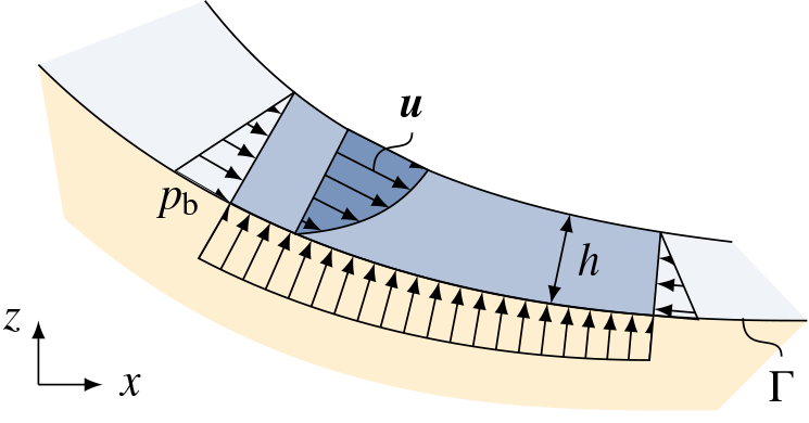
https://www.geosci-model-dev.net/11/2923/2018/gmd-11-2923-2018-f01

Figure 1Definition of velocity u, flow thickness h and basal pressure p_b on a control volume. A hydrostatic and linear pressure distribution is assumed. The shape of the velocity profile is commonly ignored in governing equations (Baker et al., 2016). Flow thickness h is measured normal to the basal surface Γ. The curvature radius of the surface Γ is assumed to be much bigger than the flow thickness.

Download

2.1.1 Mechanical model

A basic shallow granular flow model can be written in terms of surface partial differential equations as¹

\begin{array}{l} (1) & \frac{\partial h}{\partial t} + \nabla \cdot (h \overline{u}) = \frac{\dot{q}}{ρ}, \\ (2) & \frac{\partial (h \overline{u})}{\partial t} + \nabla_{s} \cdot (h \overline{u} \overline{u}) = - \frac{1}{ρ} τ_{b} + h g_{s} - \frac{1}{2 ρ} \nabla_{s} (h p_{b}), \\ (3) & \nabla_{n} \cdot (h \overline{u} \overline{u}) = h g_{n} - \frac{1}{2 ρ} \nabla_{n} (h p_{b}) - \frac{1}{ρ} n_{b} p_{b} . \end{array}

Equations (1) to (3) are equivalent to a Savage–Hutter-like system, consistently extended to complex but mildly curved terrain and entrainment. The notation as SPDE makes extension to complex terrain straightforward and implementation into SPDE environments, e.g. OpenFOAM, possible. A formal derivation is given by Rauter and Tuković (2018). Here, we aim to deliver a short and descriptive introduction.

Equation (1) represents the depth-integrated continuity equation, Eq. (2) the surface-tangential momentum conservation equation and Eq. (3) its surface-normal counterpart, defined at all points x_b on the surface Γ⊂ℝ³, representing the mountain surface. The time is denoted as t. The unknown fields are the surface-normal flow thickness h(x_b) (see Fig. 1), the depth-averaged flow velocity $\overline{u} (x_{b}) \in R^{3}$ , defined as

\begin{matrix} (4) & \overline{u} (x_{b}) = \frac{1}{h (x_{b})} \int_{0}^{h (x_{b})} u (x_{b} - n_{b} z^{'}) d z^{'}, \end{matrix}

and the basal pressure p_b(x_b). The density ρ is assumed to be constant. Note that the earth pressure theory (e.g. Savage and Hutter, 1989, 1991) has been replaced with the hydrostatic pressure assumption, as in most practical applications (e.g. Christen et al., 2010). Moreover, Eqs. (1) to (3) are written in conservative form. Therefore, there is no entrainment term in Eq. (2), which would show up in a non-conservative formulation. The first terms in Eqs. (1) and (2) represent the temporal derivative, i.e. the local change in mass and momentum, respectively. The second terms in Eqs. (1) and (2) are the respective advection terms. The right-hand side of Eq. (1) represents mass growth due to entrainment. The first, second and third terms on the right-hand side of Eq. (2) represent surface-tangential components of basal friction, gravitational acceleration and lateral pressure gradient, respectively. The surface-normal components of these terms appear in the surface-normal momentum conservation equation (Eq. 3). This equation is used to calculate the basal pressure, represented by the last term.

In the framework of SPDEs, the normal vector field n_b(x_b)∈ℝ³ of the surface Γ is sufficient to describe all major curvature effects. This is realised by calculating all contributions to conservation equations in the global coordinate system and projecting results onto the surface and the surface-normal vector. These projections are explained in detail in Appendix A. Surface-tangential and normal components contribute to local acceleration and basal pressure, respectively. This follows from the assumption that movement is constrained in surface-normal direction, which is enforced by a mechanical force, namely the basal pressure. The gravitational acceleration g, for example, is split into a surface-tangential component,

\begin{matrix} (5) & g_{s} = (I - n_{b} n_{b}) \cdot g, \end{matrix}

and a surface-normal component,

\begin{matrix} (6) & g_{n} = (n_{b} n_{b}) \cdot g . \end{matrix}

The gradient operator ∇ denotes the three-dimensional derivative along the surface (Deckelnick et al., 2005). If the responding result is a three-dimensional vector field (e.g. gradient of a scalar field or divergence of a tensor field), it can be split, similar to the gravitational acceleration, into a surface-tangential component,

\begin{matrix} (7) & \nabla_{s} = (I - n_{b} n_{b}) \cdot \nabla, \end{matrix}

and a surface-normal component,

\begin{matrix} (8) & \nabla_{n} = (n_{b} n_{b}) \cdot \nabla . \end{matrix}

For simply curved surfaces, the given relation matches the model of Greve et al. (1994), as shown by Rauter and Tuković (2018).

2.1.2 Process models

There are various user-selectable models, describing basal friction τ_b(x_b) and entrainment rate $\dot{q} (x_{b})$ , to close the system of equations. To reassemble the traditional model Christen et al. (often called Voellmy or Voellmy–Salm model; 2010), as applied, for example, by Fischer et al. (2015), the basal friction is described following Voellmy (1955),

\begin{matrix} (9) & τ_{b} = μ p_{b} \frac{\overline{u}}{| \overline{u} | + u_{0}} + \frac{ρ g}{ξ} | \overline{u} | \overline{u} . \end{matrix}

Therein, μ and ξ are constant parameters, although they may depend on avalanche size and surface roughness (Salm et al., 1990) or flow regime (Köhler et al., 2016). The small value u₀ ( $10^{- 7} m s^{- 1}$ here) avoids divisions by zero and regularises the relation near standstill, where the original function is discontinuous. This regularisation, combined with the employed time integration scheme (implicit three-level second-order; Ferziger and Peric, 2002), leads to well-defined behaviour in the runout zone, where the velocity is nearly zero (Rauter and Tuković, 2018). This allows the avalanche to reach very low velocities in the runout zone, which are lower than the tolerance of the solver and thus virtually zero. For characteristic avalanche velocities, i.e. $| \overline{u} | > 100 u_{0}$ , this value has no relevant effect on the dynamic behaviour. Previously, this issue has been addressed with operator splitting and explicit stress reduction (e.g. Mangeney-Castelnau et al., 2003; Zhai et al., 2014; Mergili et al., 2017), which is not required in the proposed scheme.

The entrainment rate is calculated, based on an empirical erosive entrainment model, as

\begin{matrix} (10) & \dot{q} = \{\begin{array}{cc} \frac{τ_{b} \cdot \overline{u}}{e_{b}} & for h_{msc} > 0, \\ 0 & for h_{msc} = 0, \end{array} \end{matrix}

where e_b is the specific erosion energy (Fischer et al., 2015). Entrainment is restricted by the available mountain snow cover thickness h_msc. The initial mountain snow cover thickness is calculated following Fischer et al. (2015), using a linear approach,

\begin{matrix} (11) & h_{msc} (z) = (H_{msc} (z_{0}) + \frac{\partial H_{msc}}{\partial z} (z - z_{0})) \cos (ζ), \end{matrix}

where z is the surface elevation (corresponding to the vertical coordinate in the numerical model) and z₀ is the elevation of a reference station, which has to be provided by the user, alongside with the base value H_msc(z₀) and the growth rate $\frac{\partial H_{msc}}{\partial z}$ . ζ is the angle between the gravitational acceleration and the surface-normal vector. Its further evolution is described by the conservation equation

\begin{matrix} (12) & \frac{\partial h_{msc}}{\partial t} = - \frac{\dot{q}}{ρ} . \end{matrix}

Undershoots, i.e. h_msc<0, are prevented with a regularisation similar to Eq. (9). This can be realised by multiplying the entrainment rate $\dot{q}$ with $\frac{h_{msc}}{h_{msc} + h_{0}}$ , where h₀ is a small value, similar to u₀.

2.1.3 Numerical solution

The governing equations are solved with an implicit, conservative, finite-area method (Rauter and Tuković, 2018), using the respective OpenFOAM library (Tuković and Jasak, 2012). The finite-area method is similar to the well-known finite-volume method Jasak (e.g. 1996) but with appropriate differential operators for SPDEs: Eqs. (7) and (8). We apply first- (upwind scheme) and second-order accurate spatial differencing schemes. First-order schemes converge more slowly in terms of mesh refinement due to their high numerical diffusivity. However, they effectively prevent oscillations and increase the stability of the solver. Oscillations in second-order accurate simulations are prevented with a normalised variable diagram (NVD) scheme for unstructured meshes, known as the Gamma scheme (Jasak et al., 1999). NVD schemes blend upwind and a higher-order scheme to combine advantages of both methods.

As mentioned before, OpenFOAM utilises capabilities of C++ to make top-level source code appear similar to the tensor notation of partial differential equations. The conservation equation (Eq. 1), for example, can be solved with the following lines of code using OpenFOAM:

faScalarMatrix hEqn (
    fam::ddt(h)
  + fam::div(phis, h)
 ==
    dqdt/rho
); hEqn.solve();

phis is the velocity edge field (see Rauter and Tuković, 2018, for details), and dqdt is the source term incorporating entrainment. Momentum conservation equations (Eqs. 2 and 3) look similar (see Rauter and Tuković, 2018), and conservation equations for arbitrary fields (e.g. random kinetic energy, Bartelt et al., 2016) can be added with the same syntax.

2.2 Simulation evaluation

We use an established implementation of the same flow model, SamosAT (version 2017_07_05) (Sampl and Zwinger, 2004; Sampl and Granig, 2009), for comparison. The main difference between SamosAT and the presented OpenFOAM solver is the solution method. SamosAT solves similar governing equations, slightly adapted to fit into the respective framework, with smoothed-particle hydrodynamics (SPH). This approach follows a Lagrangian description, making the handling of complex terrain simpler (Sampl and Zwinger, 2004). Therefore, SamosAT provides an excellent reference to validate avalanche models for complex terrain. The second term on the right-hand side of Eq. (3) was deactivated in OpenFOAM computations to reassemble the mechanical model as implemented in SamosAT. This term is usually small and can be safely neglected (Rauter and Tuković, 2018). However, it is shown in equations to preserve the similarity between Eqs. (2) and (3).

We compare simulations using the 1 kPa isoline of the dynamic peak pressure, defined as

\begin{matrix} (13) & p_{dyn} (x_{b}) = max_{t} (ρ | \overline{u} (x_{b}, t) |^{2}) . \end{matrix}

Definitions of hazard zones are based on this threshold in many European countries (Jóhannesson et al., 2009) and are therefore often used for the evaluation of relevant models (e.g. Fischer et al., 2015; Rauter et al., 2016).

In addition to the comparison with a reference implementation, we present a comparison with historical records from a catastrophic event. A common method to document avalanches is the delineation of deposition. This information is also available for the presented case study. Deposition processes are not explicitly included in the flow model due to depth integration. However, the general form and size of the deposition should be reproduced by the model to be useful for hazard zone mapping. This is problematic in some implementations, e.g. SamosAT, due to missing regularisation of the friction term, but it is possible with the proposed method.

We apply model parameters (μ, ξ, e_b) optimised for SamosAT (Fischer et al., 2015), and the comparison is conducted on a qualitative level.

Finally, we evaluate OpenFOAM simulations with regard to convergence during mesh refinement to give a quantitative estimation of numerical uncertainties as recommended by Roache (1997). The numerical solution should converge to the unknown analytical solution with increasing grid resolution, and the numerical uncertainty should decay with the order of the applied method. Richardson extrapolation allows us to estimate the numerical uncertainty, using results of three different meshes. This way, the expected convergence can be verified and the numerical uncertainty quantified.

2.3 Simulation set-up

The precondition to conduct simulations in OpenFOAM is a mesh, describing the geometry of the problem. For SPDEs, e.g. shallow flow models, a surface mesh, matching the slope topography, is sufficient and no volume mesh is required. In practice, however, three-dimensional meshing tools can be used to create a volume mesh, the boundary of which can be used as surface mesh.

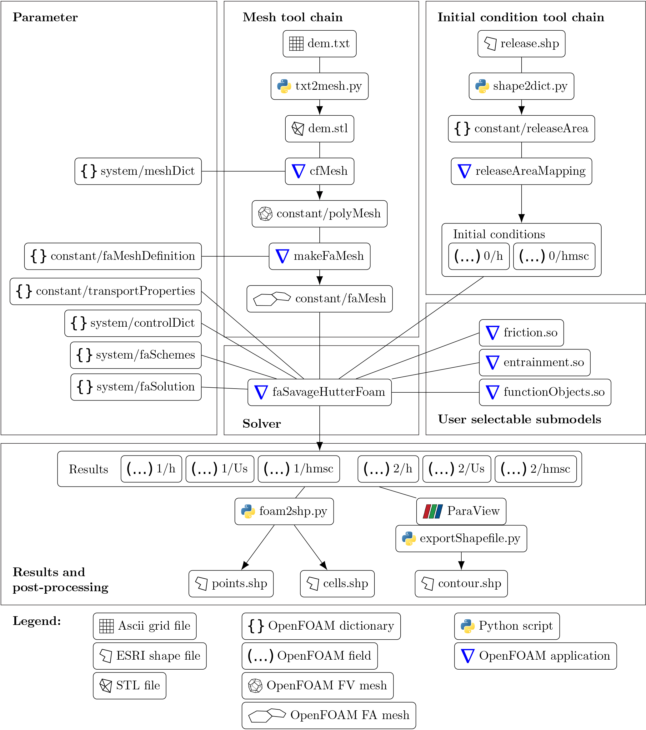
https://www.geosci-model-dev.net/11/2923/2018/gmd-11-2923-2018-f02

Figure 2Simulation set-up and tool chain. The tool chain consists exclusively of open-source applications. Individual applications and process models can be replaced with custom ones. Parameters for python scripts are provided via a command line interface. Parameters for OpenFOAM applications are provided through OpenFOAM dictionaries. Domain decomposition and reconstruction, which is handled by separate applications, is not shown. OpenFOAM reads initial conditions from the folder “0” and writes results to folders named after the corresponding time step (“1”, “2”, etc.). Details on OpenFOAM formats can be found in OpenCFD Ltd. (2004).

Download

Topography is usually available as a digital elevation model (DEM) in GIS formats, yielding elevation on a regular two-dimensional grid. The relevant part of the topography is re-sampled with cubic splines, triangulated and stored as an STL file (e.g. Kai et al., 1997) to prepare it for meshing. We chose the meshing application cfMesh (Juretić, 2015) because of its good integration in OpenFOAM and its clean boundary meshes. cfMesh requires a closed triangulated surface to create a volume mesh. This is the case for all general purpose meshing tools, and cfMesh can be replaced easily in our tool chain, for example with Netgen (Schöberl, 1997) (see Rauter and Tuković, 2018, for an application). Various other meshing tools can be applied and OpenFOAM provides a large range of mesh conversion tools. The closed surface can be assembled from a triangulation of the mountain surface, sidewalls and the respective top boundary. The resulting surface and volume mesh are presented in Fig. 3b and c. Refinement near the mountain surface reduces the amount of required volume cells, while keeping the number of surface cells high. The resulting mesh is also valid for three-dimensional simulations with, for example, Navier–Stokes equations, as conducted by, for example, Sampl and Zwinger (2004), Dutykh et al. (2011), Kröner (2013), von Boetticher et al. (2016), von Boetticher et al. (2017) and Huang et al. (2005). The boundary mesh, describing the mountain surface, is shown in Fig. 3d. The shallow flow model is solved on this surface mesh. We used polygonal-dominated (or volumetric polyhedral-dominated) meshes for simulations for stability and accuracy reasons (Juretić, 2005). Triangular (or volumetric tetrahedral) meshes have been evaluated as well. However, second-order accurate simulations on triangular meshes failed, while first-order accurate simulations are virtually identical to the respective simulations on polygonal-dominated meshes.

The release area, acting as an initial condition, is provided as a polygon in an ESRI shape file format (ESRI, 1998). To find all surface cells within the given polygon, the Hormann and Agathos (2001) algorithm as implemented in OpenFOAM is applied. The mountain snow cover h_msc of the corresponding cells is then transferred to the flow thickness h to create a suitable initial condition. The release area for our case study, taken from Fischer et al. (2015), is shown in Fig. 7a as a polygon and as a set of surface cells in Fig. 3d.

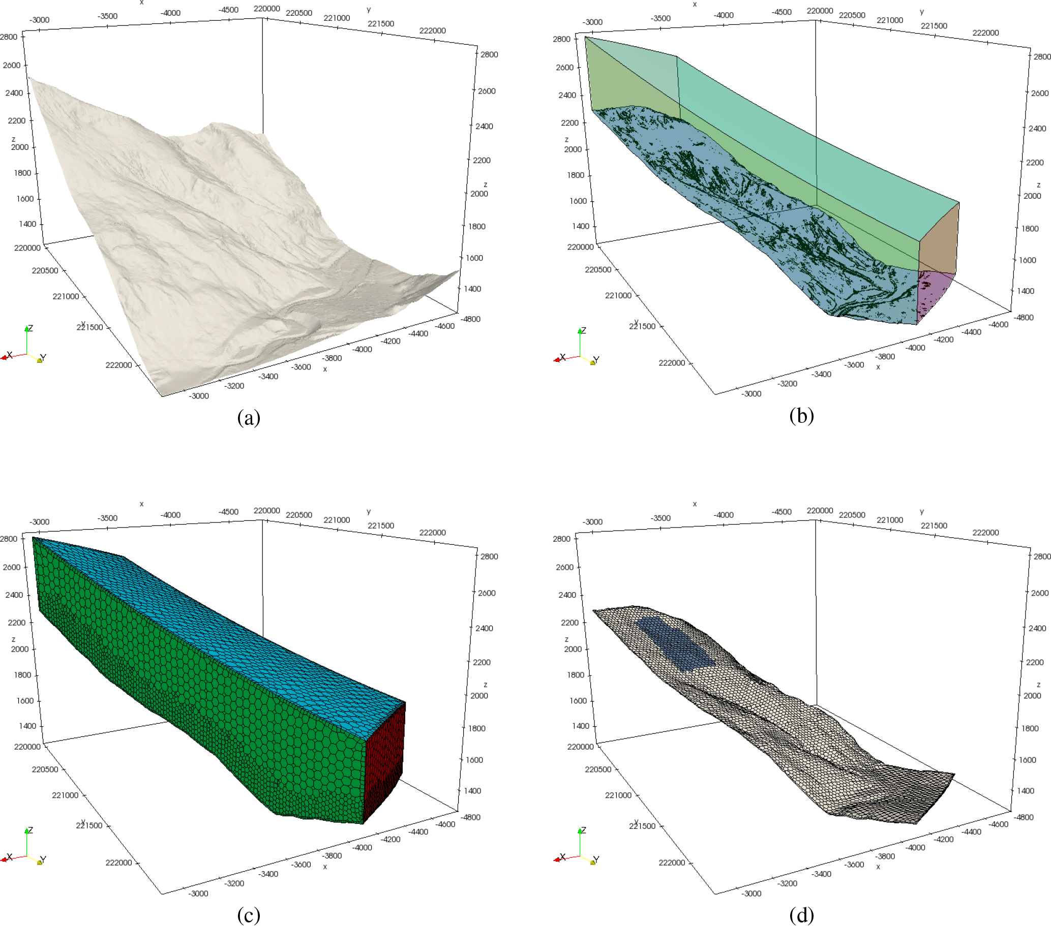
https://www.geosci-model-dev.net/11/2923/2018/gmd-11-2923-2018-f03

Figure 3Meshing tool chain: the terrain data are usually available as raster data (a). Triangulation of the relevant area and adding walls and a top boundary yields a closed triangulated surface (b; sharp edges are highlighted black). This surface can be processed by most meshing tools; here, we apply cfMesh to get a polyhedral-dominated finite-volume mesh (c). The bottom boundary surface of the finite-volume mesh builds the foundation for the finite-area mesh used for simulations (d). Note that we show a very coarse mesh for the sake of visibility of the edges. Terrain data: Amt der Tiroler Landesregierung (AdTLR). EPSG coordinate reference system: 31254.

Download

https://www.geosci-model-dev.net/11/2923/2018/gmd-11-2923-2018-f04

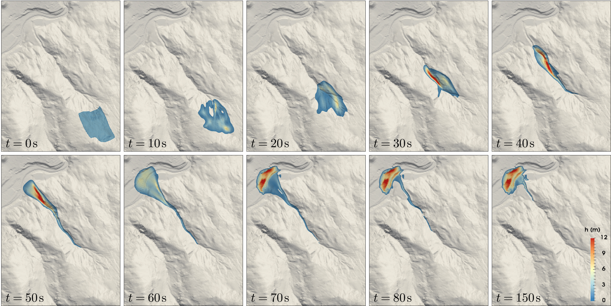
Figure 4Time series of an OpenFOAM simulation with mean cell size Δ=7.45 m and first-order interpolations in ParaView. The colour scale represents flow thickness, which is clipped at 0.5 m. Terrain data: AdTLR.

Download

The solver reads the surface mesh and initial conditions, as well as physical models, numerical schemes and constants to initialise the simulation (see Fig. 2). The respective entries can be found in the designated locations, according to the usual practice in OpenFOAM (OpenCFD Ltd., 2004). The solver can run on multiple processors using domain decomposition (Weller et al., 1998) and message passing interface (MPI).

User-defined friction and entrainment models can be loaded at run-time, meaning that the user does not have to recompile the solver to add a custom friction or entrainment model. The same is the case for general purpose functions which are triggered at the end of every time step. Here, we used this interface to calculate and record the dynamic peak pressure at run-time, without the necessity to save multiple time steps or to change solver source code. Similar functions can be used to check mass, momentum or energy conservation, record specific data (e.g. time line at a certain point), or to manipulate fields during run-time, e.g. to trigger secondary slabs.

Simulation results are written to hard disk in the usual OpenFOAM file format (OpenCFD Ltd., 2004) for post-processing, evaluation and simulation restart. The simulation set-up, all involved applications, and all intermediate and final files are presented in Fig. 2. The tool chain is modularly assembled from various open-source applications. Single modules, such as mesher, solver or friction model, can be replaced easily.

2.4 Post-processing and visualisation

Post-processing and visualisation of OpenFOAM simulations is commonly performed using ParaView^® (Ahrens et al., 2005; Ayachit, 2015) (see Figs. 3, 4 and 5). ParaView is an open-source data analysis and visualisation application. It can read and visualise OpenFOAM files, and they can be used for further operations, such as the calculation of contour lines. To integrate GIS applications in post-processing, results can be exported to common GIS file formats. Contour lines can be exported to ESRI shape file format with a custom python extension based on the library pyshp (Figs. 6c, 7 and 9). Alternatively, individual cells and respective field values can be exported as polygons (Fig. 6a) or points (Fig. 6b) to ESRI shape files.

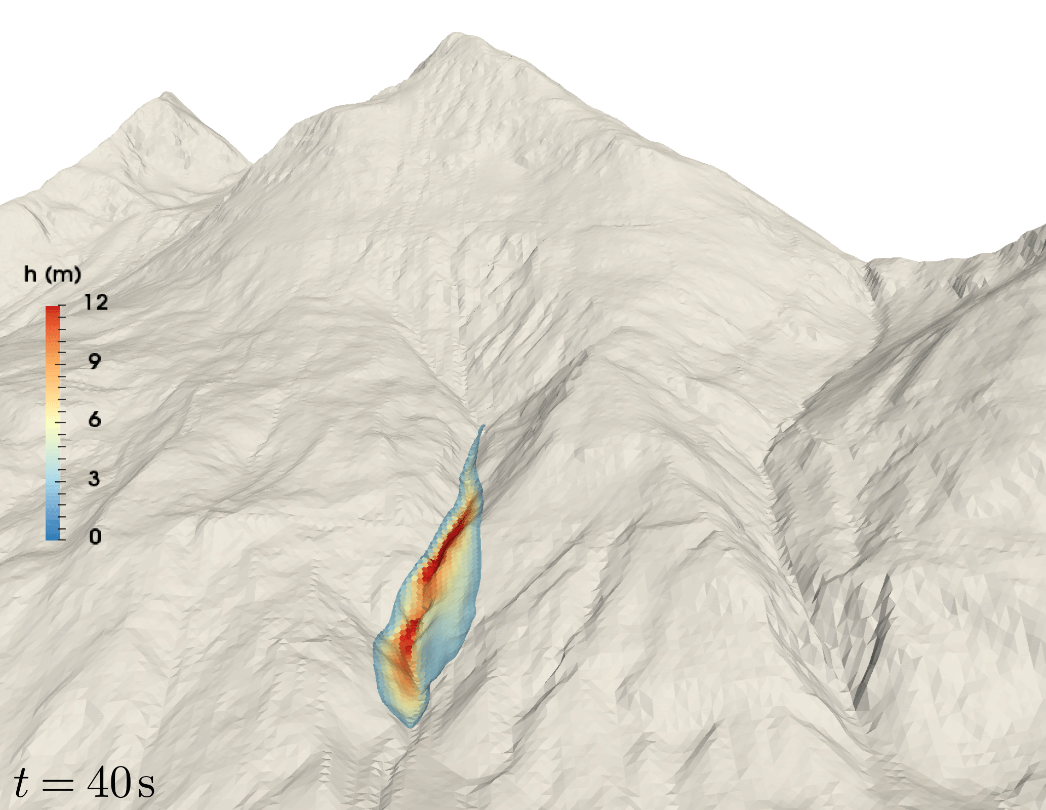
https://www.geosci-model-dev.net/11/2923/2018/gmd-11-2923-2018-f05

Figure 5Perspective view on the OpenFOAM simulation with mean cell size Δ=7.45 m and first-order interpolations in ParaView. The colour scale represents flow thickness, which is clipped at 0.5 m. Terrain data: AdTLR.

Download

https://www.geosci-model-dev.net/11/2923/2018/gmd-11-2923-2018-f06

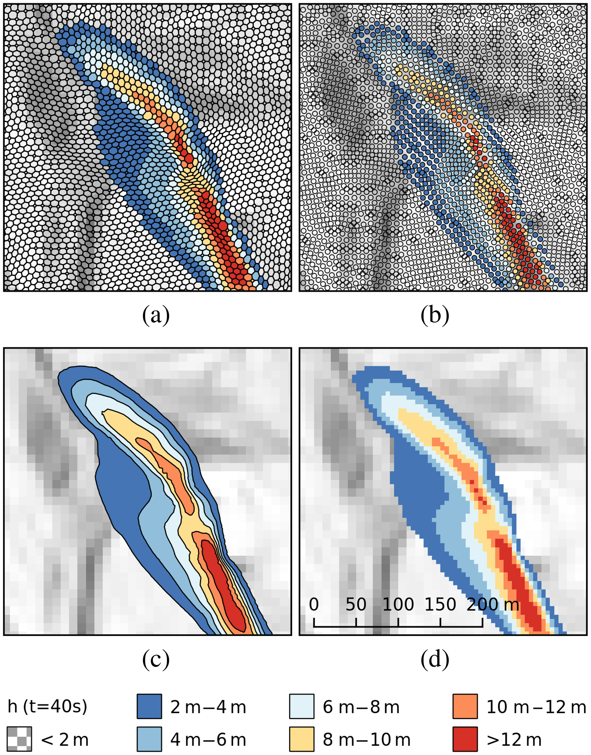
Figure 6The flow thickness field h at time t=40 s for a simulation with mean cell size Δ=7.45 m; first-order interpolations. The figure shows four methods to export and analyse results in GIS: export of cells as polygons (a); export of cell centres as points (b); export of contour lines as polygons (c); remapping of the unstructured finite-area mesh to a regular raster (d). The raster has been created by converting point data to a raster file in QGIS. The resolution of the DEM is 10 m, results have been mapped to a 5 m grid. Terrain data: AdTLR.

Download

To generate regular raster files, the unstructured OpenFOAM mesh and associated fields have to be mapped to a structured Cartesian grid (Figs. 6d and 9). These and other approaches allow an almost seamless integration into general purpose GIS applications, as shown in the following case study. Here, we utilise foam-extend-4.0 with a custom solver, python 2.7.12 with numpy 1.11.0, scipy 0.17.0 and pyshp 1.2.3 for shape file export, ParaView 5.0.1, and QGis 2.8.6.

3 Case study

In this work we focus on the Wolfsgruben avalanche. The event from 13 March 1988, when the avalanche struck inhabited areas, has been repeatedly used as benchmark for avalanche simulations, most recently by Fischer et al. (2015). We chose this example because the relevant data are freely available, making reproduction and cross-validation possible.

The mountain snow cover thickness for the specific event can be described with the parameters H_msc(z₀)=1.61 m, z₀=1289 m and $\frac{\partial H_{msc}}{\partial z} = 8 \times 10^{- 4}$ . Physical parameters to reassemble the runout properly are μ=0.26, ξ=8650 m s⁻² and $e_{b} = 11 500 J {kg}^{- 1}$ . These parameters were optimised in a previous study using SamosAT (Fischer et al., 2015).

Numerical parameters for OpenFOAM (see Rauter and Tuković, 2018) have been chosen such that they do not influence the results, while keeping the solver as stable as possible. The appropriate mesh resolution for OpenFOAM has been identified using a mesh refinement study, which is presented alongside the results. The simulation duration has been set to 150 s. This duration is sufficient to reach standstill (i.e. a velocity lower than the solver tolerance, $| \overline{u} | < 10^{- 5} m s^{- 1}$ ) in the runout zone and thus virtually unchanging deposition. We decomposed the simulation domain into four parts for OpenFOAM and all simulations have been conducted on a Quadcore Intel Core i7-7700K @ 4.20 GHz and 32 GB DDR4 Ram @ 2.667 GHz.

SamosAT utilises a grid with 5 m resolution, and we follow recommendations in terms of appropriate particle numbers and other numerical parameters. The interpolation method has been varied between interpolation on a grid (SPH-mode 0) and interpolation on particles (SPH-mode 1) to get an insight into the numerical uncertainty.

ParaView renderings are presented in Fig. 4 for multiple time steps, showing the dynamic behaviour of the avalanche. A perspective ParaView rendering is shown in Fig. 5. The avalanche follows the narrow channel directly beneath the release area. Small portions of the avalanche overflow the left and right humps in some simulations, which can be seen in the peak dynamic pressure (Fig. 7).

The results at time step t=40 s have been exported to QGIS using various methods; see Fig. 6. Affected areas (i.e. 1 kPa isolines), as predicted by OpenFOAM and SamosAT, are shown in Fig. 7. Variations due to different interpolation schemes are shown for both implementations to give an insight into the numerical uncertainty.

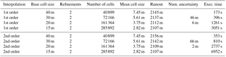
The influence of the mesh resolution on the affected area is shown in Fig. 8 for the OpenFOAM solver. Respective mean cell sizes, an estimation of the numerical uncertainty following Roache (1997) and execution times (excluding time for mesh generation, which may take several minutes) are presented in Table 1. Here, the runout is defined as the length of the central avalanche path (see Fig. 8) within the affected area. The central avalanche path has been taken from Fischer et al. (2015). The mean cell size is defined as the square root of the mean cell area. For comparison, execution times for SamosAT are 98 s (SPH-mode 0) and 368 s (SPH-mode 1). One should keep in mind that SamosAT only utilises a single processor core while OpenFOAM utilises all available cores. Moreover, execution times should be seen as rough estimates because they depend on various factors, such as the number of saved time steps, debug messages and compile options.

Table 1Mesh size, runout, error estimation and execution time for different OpenFOAM simulations. Base cell size and refinements refer to parameters of cfMesh.

Download Print Version | Download XLSX

Deposition (i.e. flow thickness field h in the last time step) of the OpenFOAM solution is shown in Fig. 9 alongside with the documentation.

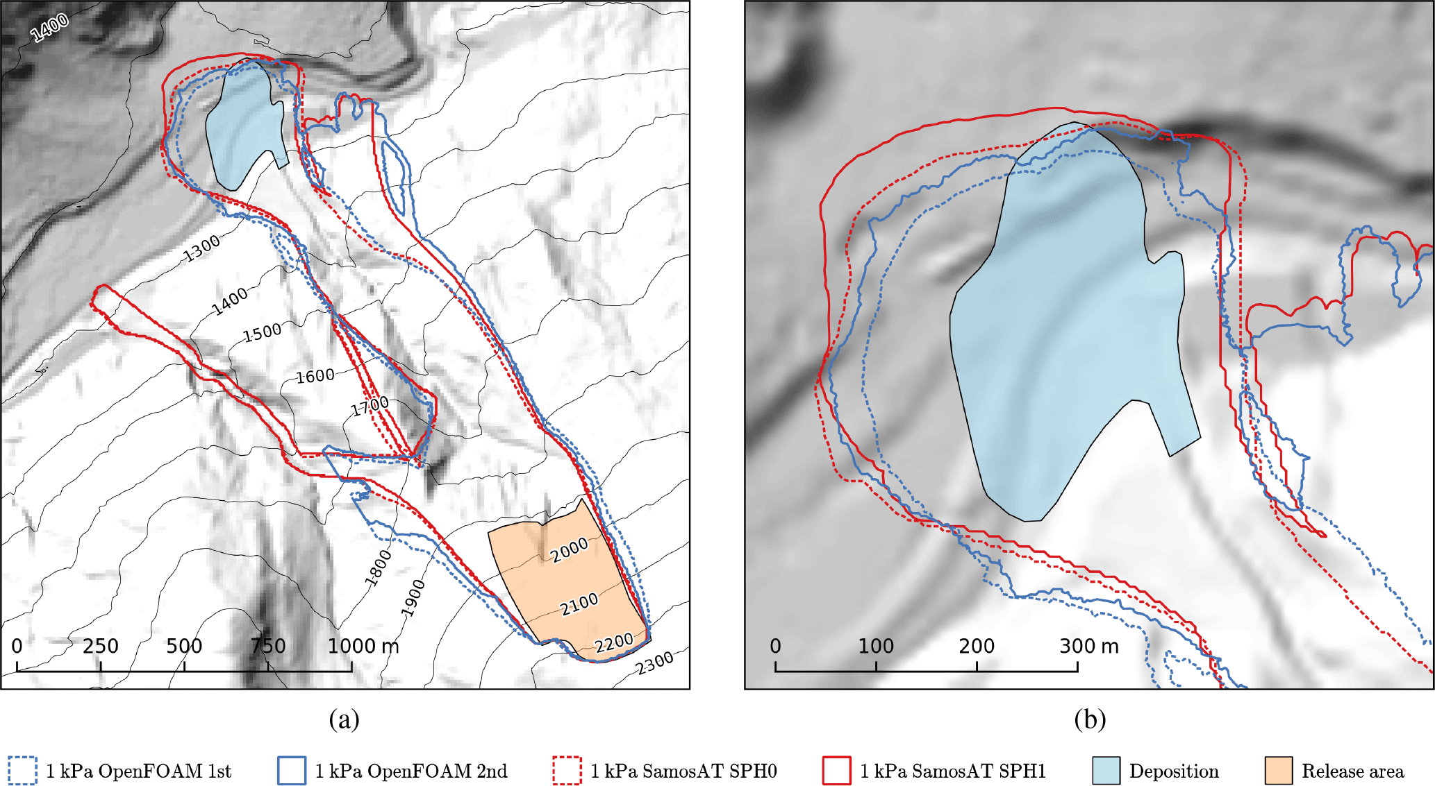
https://www.geosci-model-dev.net/11/2923/2018/gmd-11-2923-2018-f07

Figure 7Comparison of OpenFOAM first order (blue, dashed), OpenFOAM second order (blue), SamosAT SPH 0 (red, dashed) and SamosAT SPH 1 (red) in terms of 1 kPa isolines (affected area). OpenFOAM results are based on the mesh with cell size Δ=7.45 m. The documented release area (orange area) and documented deposition area (blue area) are shown for orientation. The shape and reach of the main avalanche branch are similar in all simulations; secondary branches differ to some extent. Overview (a) and focus on the runout zone (b). Terrain data: AdTLR.

Download

https://www.geosci-model-dev.net/11/2923/2018/gmd-11-2923-2018-f08

Figure 8Mesh refinement and convergence study for the OpenFOAM solver. Four mesh sizes and both interpolation schemes, first-order upwind (dashed line) and second-order Gamma (solid line) have been evaluated. The central avalanche path from Fischer et al. (2015) is shown in black. Terrain data: AdTLR.

Download

https://www.geosci-model-dev.net/11/2923/2018/gmd-11-2923-2018-f09

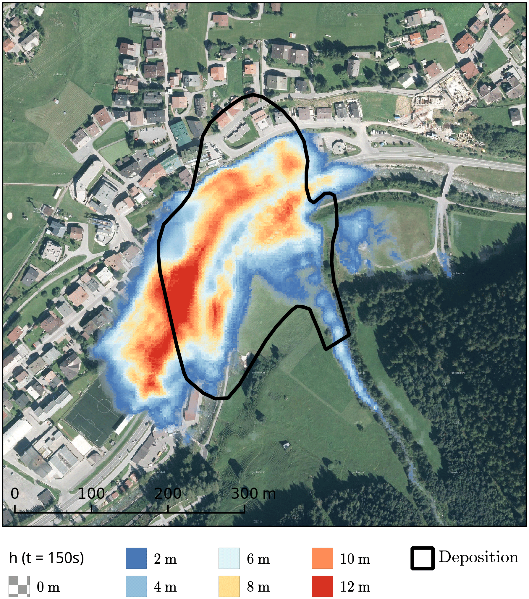
Figure 9Flow thickness field h at t=150 s of the second-order OpenFOAM simulation (Δ=3.75 m) and the documented deposition area. The flow thickness field in the last time step should roughly replicate the deposition. The bulge on the orographic right side of the deposition area is not matched by any simulation. However, some interesting details, such as the tail of the avalanche are represented well in OpenFOAM simulations. Map data: http://basemap.at (last access: 1 March 2018).

Download

4 Discussion and conclusion

Results of the new OpenFOAM solver are very similar to SamosAT. Differences between SamosAT and OpenFOAM are in the range of numerical uncertainty, and differences between interpolation methods are of a comparable size. This uncertainty has to be expected; in fact, it is well known in the CFD community that numerical schemes and implementation details influence results if they are not converged to the analytical solution (e.g. Ferziger and Peric, 2002). In the case of gravitational mass flows, numerical uncertainty plays a minor role, since underlying models, parameters, terrain and snow cover data are affected by substantially higher uncertainty. This is shown by a comparison of the documented deposition with the result of an OpenFOAM simulation in Fig. 9. Although parameters have been optimised to the specific event, all simulations differ significantly from documentation. In particular, the large bulge on the orographic right side of the deposition area is not matched by any simulation. However, some details, such as the form of the tail and the position where the deposition expands, are accurately simulated by the OpenFOAM solver. Significant differences between simulation and documentation are not limited to the presented case and have been observed before, for example, by Rauter et al. (2016). We deduce that numerical errors are much smaller than the expected model error. Under these circumstances, a quantitative comparison between implementations (as, for example, by Rauter et al., 2016, for basal friction models) is not appropriate.

The refinement study shows that in the presented case, the simulated runout reduces with increasing mesh refinement (Fig. 8). Simulations on fine meshes are stopped by the first embankment, simulations on coarser grids overflow it and reach the next embankment. This is reasonable, considering the higher diffusivity and lower curvature of coarser meshes. However, this trend should not be taken for granted for other cases and a refinement study should always be conducted to get an insight into the numerical uncertainty. Results indicate that a cell size of approximately 3.75 m is required in OpenFOAM to achieve convergence with respect to practical applications. The numerical uncertainty cannot be calculated for the coarsest and finest mesh, since three simulations are required to conduct a Richardson extrapolation. It has to be noted that all simulations are based on the same DEM with a grid size of 10 m. The influence of terrain model quality (see, e.g., Bühler et al., 2011) on simulation results is not investigated.

The execution time of the OpenFOAM solver is acceptable for coarse meshes but increases with the square of the number of cells because the time step duration has to be reduced similarly to cell size. The OpenFOAM solver is noticeably slower than SamosAT, especially when considering OpenFOAM's multiprocessing capabilities. For applications where fast execution is imperative, such as parameter studies, SamosAT may be the appropriate choice. There is potential for future optimisation in OpenFOAM; in particular, the implicit time integration scheme is expensive and should be replaced with a simpler explicit one. However, the implicit solution strategy, in combination with the regularised friction relation, leads to satisfying behaviour in the runout zone. In contrast, the simple explicit solution strategy, for example from SamosAT, leads to a continuous creeping of the deposition, meaning that the final flow thickness cannot be compared with the deposition, as noted by Fischer et al. (2015) and Rauter et al. (2016).

The stability of the OpenFOAM solver is strongly influenced by mesh quality. Simulations with polygonal-dominated surface meshes showed an acceptable stability for first- and second-order interpolations. The high influence of the three-dimensional mesh on stability and its computationally expensive creation is the main drawback of the proposed method. This is, however, also a big advantage, allowing simple coupling with three-dimensional ambient flows, as conducted by Sampl and Zwinger (2004).

5 Summary and outlook

This paper shows the application of a finite-area scheme for shallow granular flows (Rauter and Tuković, 2018) to snow avalanches on natural terrain. Specific processes, such as entrainment, have been added to the basic model to replicate the traditional model as implemented in SamosAT (Fischer et al., 2015).

Various simulations with the new OpenFOAM solver have been conducted. Methods and tools to incorporate the OpenFOAM solver in GIS have been presented. These tools allow the integration of OpenFOAM in hazard mapping workflows and thus the validation of the OpenFOAM solver with a reference implementation, herein SamosAT.

The application of three-dimensional Cartesian coordinates allows simple coupling with GIS applications because no coordinate transformations are required. Unstructured meshes, on the other hand, require re-sampling to structured meshes or data transfer in the form of polygons. This incorporates an additional effort compared to simulations on structured meshes, as conducted for example by Christen et al. (2010).

The OpenFOAM solver roughly reproduces the results of SamosAT. Differences are within the expected numerical uncertainty. A comparison of numerical results to a documented event suggests that model uncertainty is substantially higher than numerical uncertainties.

The major advantage of OpenFOAM is the object-oriented open-source code, which can be extended easily. The flexible code structure allows fast application of new models to real case examples. This especially qualifies the proposed method for model development and academic purposes. Moreover, the vast majority of source code is shared within the OpenFOAM community, leading to faster development of core features and higher code quality.

The finite-area scheme allows a description in terms of surface partial differential equations (Deckelnick et al., 2005), which leads to simple and expressive governing equations. However, this comes at the cost of a complex three-dimensional surface mesh. The projection of the governing equations on a plane surface following, for example, Bouchut and Westdickenberg (2004) may be beneficial for some applications. The three-dimensional surface mesh can also be an advantage, allowing a simple coupling with three-dimensional ambient two-phase models for powder clouds (Sampl and Zwinger, 2004). The presented meshing method, creating a finite-volume and the corresponding finite-area mesh, is viable for such simulations as well.

Future steps will incorporate the optimisation of the solver in terms of stability and execution time. Mesh generation and the integration of geographic information systems will be further streamlined. The limitation to mildly curved terrain should be eliminated, as this assumption is violated in many practical cases. We aim to implement more complex models, suitable for mixed snow avalanches (e.g. Bartelt et al., 2016; Issler et al., 2018) and debris flow (e.g. Iverson and George, 2014; Mergili et al., 2017) in the near future. Coupling of the dense flow model proposed here with three-dimensional two-phase models for the powder cloud regime (e.g. Cheng et al., 2017; Chauchat et al., 2017) is planned as well.

Code and data availability

The OpenFOAM solver, core utilities and the case study presented are available in the OpenFOAM community repository (https://develop.openfoam.com/Community/avalanche, last access: 1 March 2018) and integrated as a module within OpenFOAM-v1712. The complete code (based on foam-extend-4.0), including python scripts for GIS integration and the simulation set-up including the underlying raw data, is included in the Supplement and available at https://bitbucket.org/matti2/fasavagehutterfoam (last access: 1 March 2018).

Appendix A: Understanding projections in surface partial differential equations

Here we briefly explain the concept of projections within the framework of surface partial differential equations. These projections are widely used in computational fluid dynamics, usually when surfaces in three-dimensional space are considered. We do not focus on mathematical formalities and this section cannot replace the formal derivation of Rauter and Tuković (2018). We want to emphasise that no surface-aligned coordinate system is required throughout the whole process, and the reader is encouraged to adhere to global Cartesian coordinates. For simplicity we present a discretised finite-area cell, which has been extruded by flow thickness h to present the flowing mass; see Fig. A1.

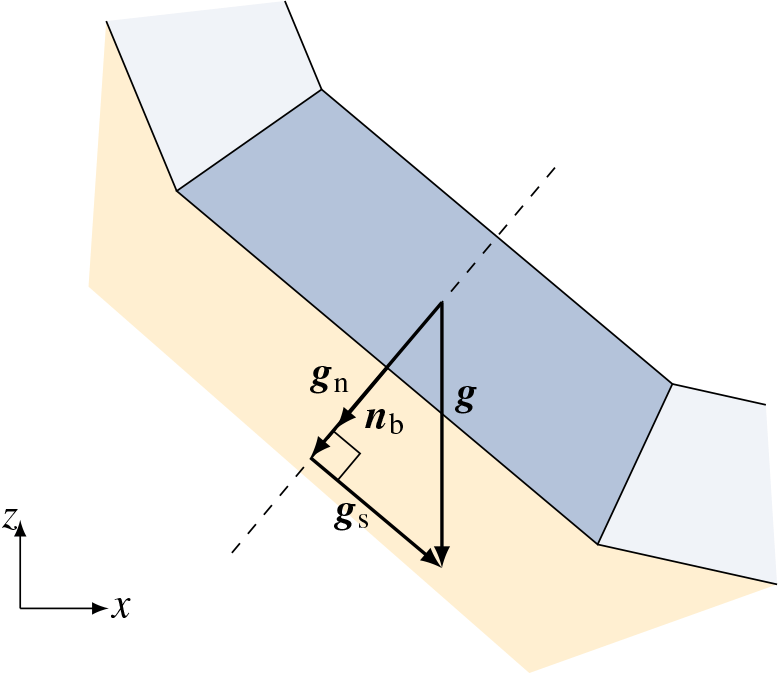
https://www.geosci-model-dev.net/11/2923/2018/gmd-11-2923-2018-f10

Figure A1Splitting gravitational acceleration into a surface-tangential and surface-normal part with simple projections to the surface-normal vector n_b.

Download

We begin by splitting a simple vectorial entity, the gravitational acceleration g∈ℝ³, into a surface-normal component, g_n∈ℝ³, and a surface-tangential component, g_s∈ℝ³, as shown in Fig. A1. The magnitude of the surface-normal component can be calculated using the scalar product and the surface-normal vector:

\begin{matrix} (A1) & ‖ g_{n} ‖ = n_{b} \cdot g, \end{matrix}

which corresponds to a projection of g on n_b. The surface-normal component points in the same direction as the surface-normal vector, which allows the calculation of the vectorial surface-normal component. Rearranging of vector multiplications yields the known form

\begin{matrix} (A2) & g_{n} = n_{b} ‖ g_{n} ‖ = n_{b} (n_{b} \cdot g) = (n_{b} n_{b}) \cdot g . \end{matrix}

The surface-tangential component follows by subtracting the surface-normal component from total gravitational acceleration:

\begin{matrix} (A3) & g_{s} = g - g_{n} = g - (n_{b} n_{b}) \cdot g = (I - n_{b} n_{b}) \cdot g . \end{matrix}

Movement in surface-normal direction is constrained by the basal topography, which yields the basal pressure. Therefore, the surface-normal component g_n has to contribute to basal pressure p_b (Eq. 3), and only the surface-tangential component contributes to local acceleration $\frac{\partial h \overline{u}}{\partial t}$ (Eq. 2). The total gravitational acceleration can be reconstructed by summing up both components:

\begin{matrix} (A4) & g = g_{n} + g_{s} = (n_{b} n_{b}) \cdot g + (I - n_{b} n_{b}) \cdot g = I \cdot g = g, \end{matrix}

ensuring perfect conservation of three-dimensional momentum.

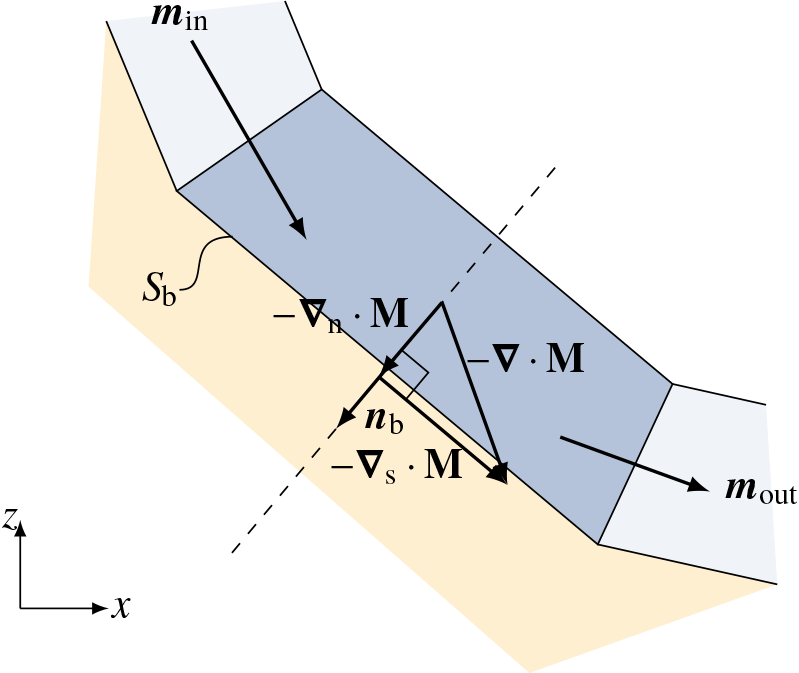
https://www.geosci-model-dev.net/11/2923/2018/gmd-11-2923-2018-f11

Figure A2Splitting the divergence of a flux tensor ∇⋅M into a surface-tangential and surface-normal part with simple projections to the surface-normal vector n_b.

Download

The same concept can be applied to fluxes through the boundary of the control volume, leading to the concept of surface partial differential operators (∇_s and ∇_n). Figure A2 shows the divergence of a tensor, ∇⋅M, which could represent convective momentum transport $\nabla \cdot (h \overline{u} \overline{u})$ or the lateral pressure gradient $\frac{1}{2 ρ} \nabla (p_{b} h) = \frac{1}{2 ρ} \nabla \cdot (I p_{b} h)$ . Using Gauss' theorem, the divergence can be reformulated in terms of the surface integral of face fluxes, which are defined as the scalar product of the flux tensor M with the normal vector on the face (Ferziger and Peric, 2002). In the discretised form, integrals are replaced with sums over faces and in the case of SPDEs, volumes collapse to surfaces, faces to edges and face fluxes to edge fluxes. For the simple case, as shown in Fig. A2, we can write

\begin{matrix} (A5) & \nabla \cdot M = \frac{1}{S_{b}} (m_{out} - m_{in}), \end{matrix}

with area of the cell S_b and edge fluxes m_in and m_out. For the exact formulation in terms of finite areas, the reader is refereed to Rauter and Tuković (2018). Note that ∇⋅M is a three-dimensional vector without any particular direction in relation to the basal surface. Hence, it has a surface-tangential and a surface-normal component which can be treated similarly to gravitational acceleration, yielding the surface-normal component

\begin{array}{l} (A6) & \nabla_{n} \cdot M = & n_{b} ‖ \nabla_{n} \cdot M ‖ = n_{b} (n_{b} \cdot \nabla \cdot M) \\ = & (n_{b} n_{b}) \cdot \nabla \cdot M, \end{array}

and the surface-tangential component

\begin{array}{l} (A7) & \nabla_{s} \cdot M = & \nabla \cdot M - \nabla_{n} \cdot M = \nabla \cdot M - (n_{b} n_{b}) \cdot \nabla \cdot M \\ = & (I - n_{b} n_{b}) \cdot \nabla \cdot M . \end{array}

Surface-normal and tangential components contribute to local acceleration and basal pressure for reasons discussed in terms of gravitational acceleration. Three-dimensional conservation is ensured for fluxes as well if ∇⋅M is calculated conservatively. Finally, we want to note that velocity is a three-dimensional vector field and its direction is not fixed a priori. However, velocity will always be aligned with the surface because only surface-tangential components are present in the respective conservation equation.

Supplement

The supplement related to this article is available online at: https://doi.org/10.5194/gmd-11-2923-2018-supplement.

Author contributions

MR developed the model and the respective code. Simulations have been conducted by MR and AK. AH covered GIS aspects and the production of respective figures. WF conceived the presented investigation, verified the underlying analytical models and supervised the project. All authors discussed the results and contributed to the final paper.

Competing interests

The authors declare that they have no conflict of interest.

Acknowledgements

We thank Mark Olesen and Andrew Heather (ESI-OpenCFD) for help regarding OpenFOAM and a review of our solver code. We thank Matthias Granig and Felix Oesterle (WLV) for support regarding SamosAT and for providing the respective software. We thank our colleges, Iman Bathaeian, Jan-Thomas Fischer and Fabian Schranz, for valuable comments on the manuscript. We thank the OpenFOAM, ParaView and QGIS communities for sharing their code and providing helpful advice. We further thank Stefan Hergarten, Julia Kowalski and one anonymous reviewer for their valuable comments, which helped to increase the clarity and quality of this paper. We gratefully acknowledge the financial support of the OEAW project “Beyond dense flow avalanches” and the Vice Rectorate for Research at the University of Innsbruck. The computational results presented have been achieved (in part) using the HPC infrastructure LEO of the University of Innsbruck.

Edited by: Simone Marras
Reviewed by: Julia Kowalski, Stefan Hergarten, and one anonymous referee

References

Ahrens, J., Geveci, B., Law, C., Hansen, C., and Johnson, C.: ParaView: An End-User Tool for Large Data Visualization, in: The Visualization Handbook, Elsevier, 717–731, 2005. a

Ancey, C.: Plasticity and geophysical flows: a review, J. Non-Newton. Fluid, 142, 4–35, https://doi.org/10.1016/j.jnnfm.2006.05.005, 2007. a

Ayachit, U.: The ParaView Guide: A Parallel Visualization Application, Kitware, Inc., 2015. a

Baker, J. L., Barker, T., and Gray, J. M. N. T.: A two-dimensional depth-averaged μ(I)-rheology for dense granular avalanches, J. Fluid Mech., 787, 367–395, https://doi.org/10.1017/jfm.2015.684, 2016. a, b

Barker, T. and Gray, J.: Partial regularisation of the incompressible μ(I)-rheology for granular flow, J. Fluid Mech., 828, 5–32, https://doi.org/10.1017/jfm.2017.428, 2017. a

Barré de Saint-Venant, A. J. C.: Théorie du mouvement non permanent des eaux, avec application aux crues des rivières et à l'introduction des marées dans leurs lits, Cr. Acad. Sci., 73, 237–240, 1871. a

Bartelt, P., Buser, O., and Platzer, K.: Fluctuation–dissipation relations for granular snow avalanches, J. Glaciol., 52, 631–643, https://doi.org/10.3189/172756506781828476, 2006. a

Bartelt, P., Buser, O., Vera Valero, C., and Bühler, Y.: Configurational energy and the formation of mixed flowing/powder snow and ice avalanches, Ann. Glaciol., 57, 179–188, https://doi.org/10.3189/2016AoG71A464, 2016. a, b, c, d

Bouchut, F. and Westdickenberg, M.: Gravity driven shallow water models for arbitrary topography, Commun. Math. Sci., 2, 359–389, 2004. a, b, c

Bühler, Y., Christen, M., Kowalski, J., and Bartelt, P.: Sensitivity of snow avalanche simulations to digital elevation model quality and resolution, Ann. Glaciol., 52, 72–80, https://doi.org/10.3189/172756411797252121, 2011. a

Chauchat, J., Cheng, Z., Nagel, T., Bonamy, C., and Hsu, T.-J.: SedFoam-2.0: a 3-D two-phase flow numerical model for sediment transport, Geosci. Model Dev., 10, 4367–4392, https://doi.org/10.5194/gmd-10-4367-2017, 2017. a

Cheng, Z., Hsu, T.-J., and Calantoni, J.: SedFoam: A multi-dimensional Eulerian two-phase model for sediment transport and its application to momentary bed failure, Coast. Eng., 119, 32–50, https://doi.org/10.1016/j.coastaleng.2016.08.007, 2017. a

Christen, M., Kowalski, J., and Bartelt, P.: RAMMS: Numerical simulation of dense snow avalanches in three-dimensional terrain, Cold Reg. Sci. Technol., 63, 1–14, https://doi.org/10.1016/j.coldregions.2010.04.005, 2010. a, b, c, d, e, f, g

Craster, R. V. and Matar, O. K.: Dynamics and stability of thin liquid films, Rev. Mod. Phys., 81, 1131–1198, https://doi.org/10.1103/RevModPhys.81.1131, 2009. a

Deckelnick, K., Dziuk, G., and Elliott, C. M.: Computation of geometric partial differential equations and mean curvature flow, Acta Numer., 14, 139–232, https://doi.org/10.1017/S0962492904000224, 2005. a, b, c, d

Denlinger, R. P. and Iverson, R. M.: Granular avalanches across irregular three-dimensional terrain: 1. Theory and computation, J. Geophys. Res.-Earth, 109, F01014, https://doi.org/10.1029/2003JF000085, 2004. a, b

Dieter-Kissling, K., Marschall, H., and Bothe, D.: Direct Numerical Simulation of droplet formation processes under the influence of soluble surfactant mixtures, Comput. Fluids, 113, 93–105, https://doi.org/10.1016/j.compfluid.2015.01.017, 2015a. a

Dieter-Kissling, K., Marschall, H., and Bothe, D.: Numerical method for coupled interfacial surfactant transport on dynamic surface meshes of general topology, Comput. Fluids, 109, 168–184, https://doi.org/10.1016/j.compfluid.2014.12.017, 2015b. a

Domnik, B., Pudasaini, S. P., Katzenbach, R., and Miller, S. A.: Coupling of full two-dimensional and depth-averaged models for granular flows, J. Non-Newton. Fluid, 201, 56–68, https://doi.org/10.1016/j.jnnfm.2013.07.005, 2013. a

Dutykh, D., Acary-Robert, C., and Bresch, D.: Mathematical Modeling of Powder-Snow Avalanche Flows, Stud. Appl. Math., 127, 38–66, https://doi.org/10.1111/j.1467-9590.2010.00511.x, 2011. a

ESRI: ESRI Shapefile Technical Description, available at: https://www.esri.com/library/whitepapers/pdfs/shapefile.pdf (last access: 17 December 2017), 1998. a

Ferziger, J. H. and Peric, M.: Computational methods for fluid dynamics, Springer, 3rd edn., 2002. a, b, c

Fischer, J.-T., Kowalski, J., and Pudasaini, S. P.: Topographic curvature effects in applied avalanche modeling, Cold Reg. Sci. Technol., 74, 21–30, https://doi.org/10.1016/j.coldregions.2012.01.005, 2012. a

Fischer, J.-T., Kofler, A., Wolfgang, F., Granig, M., and Kleemayr, K.: Multivariate parameter optimization for computational snow avalanche simulation in 3d terrain, J. Glaciol., 61, 875–888, https://doi.org/10.3189/2015JoG14J168, 2015. a, b, c, d, e, f, g, h, i, j, k, l, m

Gray, J. M. N. T., Wieland, M., and Hutter, K.: Gravity-driven free surface flow of granular avalanches over complex basal topography, P. Roy. Soc. Lond. A Mat., 455, 1841–1874, https://doi.org/10.1098/rspa.1999.0383, 1999. a

Greve, R., Koch, T., and Hutter, K.: Unconfined Flow of Granular Avalanches along a Partly Curved Surface. I. Theory, P. Roy. Soc. Lond. A Mat., 445, 399–413, https://doi.org/10.1098/rspa.1994.0068, 1994. a, b

Grigorian, S. S., Eglit, M. E., and Iakimov, Y. L.: A new formulation and solution of the problem of snow avalanche motion, Snow Avalanches Glaciers, 12, 104–113, 1967. a

Hanert, E., Le Roux, D. Y., Legat, V., and Deleersnijder, E.: An efficient Eulerian finite element method for the shallow water equations, Ocean Model., 10, 115–136, https://doi.org/10.1016/j.ocemod.2004.06.006, 2005. a

Hergarten, S. and Robl, J.: Modelling rapid mass movements using the shallow water equations in Cartesian coordinates, Nat. Hazards Earth Syst. Sci., 15, 671–685, https://doi.org/10.5194/nhess-15-671-2015, 2015. a, b, c, d

Hormann, K. and Agathos, A.: The point in polygon problem for arbitrary polygons, Comp. Geom., 20, 131–144, https://doi.org/10.1016/S0925-7721(01)00012-8, 2001. a

Huang, H., Imran, J., and Pirmez, C.: Numerical model of turbidity currents with a deforming bottom boundary, J. Hydraul. Eng., 131, 283–293, https://doi.org/10.1061/(ASCE)0733-9429(2005)131:4(283), 2005. a, b

Hungr, O.: A model for the runout analysis of rapid flow slides, debris flows, and avalanches, Can. Geotech. J., 32, 610–623, https://doi.org/10.1139/t95-063, 1995. a, b

Issler, D.: Dynamically consistent entrainment laws for depth-averaged avalanche models, J. Fluid Mech., 759, 701–738, https://doi.org/10.1017/jfm.2014.584, 2014. a

Issler, D. and Gauer, P.: Exploring the significance of the fluidized flow regime for avalanche hazard mapping, Ann. Glaciol., 49, 193–198, https://doi.org/10.3189/172756408787814997, 2008. a

Issler, D., Jenkins, J. T., and McElwaine, J. N.: Comments on avalanche flow models based on the concept of random kinetic energy, J. Glaciol., 64, 148–164, https://doi.org/10.1017/jog.2017.62, 2018. a

Iverson, R. M. and George, D. L.: A depth-averaged debris-flow model that includes the effects of evolving dilatancy. I. Physical basis, P. Roy. Soc. Lond. A Mat., 470, 20130819, https://doi.org/10.1098/rspa.2013.0819, 2014. a, b

Iverson, R. M. and George, D. L.: Modelling landslide liquefaction, mobility bifurcation and the dynamics of the 2014 Oso disaster, Géotechnique, 66, 175–187, https://doi.org/10.1680/jgeot.15.LM.004, 2016. a

Jasak, H.: Error analysis and estimation for the finite volume method with applications to fluid flows, PhD thesis, Imperial College, University of London, 1996. a

Jasak, H., Weller, H. G., and Gosman, A. D.: High resolution NVD differencing scheme for arbitrarily unstructured meshes, Int. J. Numer. Meth. Fluids, 31, 431–449, https://doi.org/10.1002/(SICI)1097-0363(19990930)31:2<431::AID-FLD884>3.0.CO;2-T, 1999. a, b

Jóhannesson, T., Gauer, P., Issler, P., and Lied, K.: The design of avalanche protection dams, Recent practical and theoretical developments, No. EUR 23339 in Climate Change and Natural Hazard Research Series 2, 978-92-79-08885-8, 2009. a

Juretić, F.: Error analysis in finite volume CFD, PhD thesis, Imperial College London, University of London, 2005. a

Juretić, F.: cfMesh User Guide, Creative Fields, Zagreb, available at: http://cfmesh.com/wp-content/uploads/2015/09/User_Guide-cfMesh_v1.1.pdf (last access: 16 June 2018), 2015. a

Kai, C. C., Jacob, G. G., and Mei, T.: Interface between CAD and rapid prototyping systems, Part 1: a study of existing interfaces, Int. J. Adv. Manuf. Tech., 13, 566–570, https://doi.org/10.1007/BF01176300, 1997. a

Köhler, A., McElwaine, J. N., Sovilla, B., Ash, M., and Brennan, P.: The dynamics of surges in the 3 February 2015 avalanches in Vallée de la Sionne, J. Geophys. Res.-Earth, 121, 2192–2210, https://doi.org/10.1002/2016JF003887, 2016. a

Kowalski, J. and McElwaine, J. N.: Shallow two-component gravity-driven flows with vertical variation, J. Fluid Mech., 714, 434–462, https://doi.org/10.1017/jfm.2012.489, 2013. a

Kröner, C.: Experimental and numerical description of rapid granular flows and some baseline constraints for simulating 3-dimensional granular flow dynamics, PhD thesis, Rheinische Friedrich-Wilhelms-Universität Bonn, available at: http://hss.ulb.uni-bonn.de/2014/3694/3694a.pdf (last access: 17 December 2017), 2013. a, b

Mangeney-Castelnau, A., Vilotte, J.-P., Bristeau, M.-O., Perthame, B., Bouchut, F., Simeoni, C., and Yerneni, S.: Numerical modeling of avalanches based on Saint Venant equations using a kinetic scheme, J. Geophys. Res.-Solid , 108, 2527, https://doi.org/10.1029/2002JB002024, 2003. a

Marschall, H., Boden, S., Lehrenfeld, C., Falconi D., C. J. Hampel, U., Reusken, A., Wörner, M., and Bothe, D.: Validation of interface capturing and tracking techniques with different surface tension treatments against a Taylor bubble benchmark problem, Comput. Fluids, 102, 336–352, https://doi.org/10.1016/j.compfluid.2014.06.030, 2014. a

Medina, V., Hürlimann, M., and Bateman, A.: Application of FLATModel, a 2D finite volume code, to debris flows in the northeastern part of the Iberian Peninsula, Landslides, 5, 127–142, https://doi.org/10.1007/s10346-007-0102-3, 2008. a

Mergili, M., Schratz, K., Ostermann, A., and Fellin, W.: Physically-based modelling of granular flows with Open Source GIS, Nat. Hazards Earth Syst. Sci., 12, 187–200, https://doi.org/10.5194/nhess-12-187-2012, 2012 a

Mergili, M., Fischer, J.-T., Krenn, J., and Pudasaini, S. P.: r.avaflow v1, an advanced open-source computational framework for the propagation and interaction of two-phase mass flows, Geosci. Model Dev., 10, 553–569, https://doi.org/10.5194/gmd-10-553-2017, 2017. a, b, c, d, e

Norem, H., Irgens, F., and Schieldrop, B.: A continuum model for calculating snow avalanche velocities, in: Proceedings of the Symposium on Avalanche Formation, Movement and Effects, Davos, Switzerland, IAHS Publication no. 162, 14–19, 1987. a

Olshanskii, M. A., Reusken, A., and Grande, J.: A Finite Element Method for Elliptic Equations on Surfaces, SIAM J. Numer. Anal., 47, 3339–3358, https://doi.org/10.1137/080717602, 2009. a

OpenCFD Ltd.: OpenFOAM – The Open Source CFD Toolbox – User Guide, available at: https://www.openfoam.com/documentation/user-guide/ (last access: 31 January 2018), 2004. a, b, c, d

Patra, A. K., Bauer, A. C., Nichita, C. C., Pitman, E. B., Sheridan, M. F., Bursik, M., Rupp, B., Webber, A., Stinton, A. J., Namikawa, L. M., and Renschler, C. S.: Parallel adaptive numerical simulation of dry avalanches over natural terrain, J. Volcanol. Geoth. Res., 139, 1–21, https://doi.org/10.1016/j.jvolgeores.2004.06.014, 2005. a

Pesci, C., Dieter-Kissling, K., Marschall, H., and Bothe, D.: Finite volume/finite area interface tracking method for two-phase flows with fluid interfaces influenced by surfactant, in: Computational Methods for Complex Liquid-Fluid Interfaces, CRC Press, Taylor & Francis Group, 373–409, https://doi.org/10.1201/b19337-22, 2015. a

Pitman, E. B., Nichita, C. C., Patra, A., Bauer, A., Sheridan, M., and Bursik, M.: Computing granular avalanches and landslides, Phys. Fluids, 15, 3638–3646, https://doi.org/10.1063/1.1614253, 2003. a

Pouliquen, O. and Forterre, Y.: Friction law for dense granular flows: application to the motion of a mass down a rough inclined plane, J. Fluid Mech., 453, 133–151, https://doi.org/10.1017/S0022112001006796, 2002. a

Pudasaini, S. P.: A general two-phase debris flow model, J. Geophys. Research.-Earth, 117, F03010, https://doi.org/10.1029/2011JF002186, 2012. a

Pudasaini, S. P. and Hutter, K.: Avalanche Dynamics: Dynamics of Rapid Flows of Dense Granular Avalanches, Springer, https://doi.org/10.1007/978-3-540-32687-8, 2007. a, b

Pudasaini, S. P., Wang, Y., and Hutter, K.: Modelling debris flows down general channels, Nat. Hazards Earth Syst. Sci., 5, 799–819, https://doi.org/10.5194/nhess-5-799-2005, 2005a. a

Pudasaini, S. P., Wang, Y., and Hutter, K.: Rapid motions of free-surface avalanches down curved and twisted channels and their numerical simulation, P. Roy. Soc. Lond. A Mat., 363, 1551–1571, https://doi.org/10.1098/rsta.2005.1595, 2005b. a

Rauter, M. and Tuković, Ž.: A finite area scheme for shallow granular flows on three-dimensional surfaces, Comput. Fluids, https://doi.org/10.1016/j.compfluid.2018.02.017, 2018. a, b, c, d, e, f, g, h, i, j, k, l, m, n, o, p

Rauter, M., Fischer, J.-T., Fellin, W., and Kofler, A.: Snow avalanche friction relation based on extended kinetic theory, Nat. Hazards Earth Syst. Sci., 16, 2325–2345, https://doi.org/10.5194/nhess-16-2325-2016, 2016. a, b, c, d, e

Roache, P. J.: Quantification of uncertainty in computational fluid dynamics, Annu. Rev. Fluid Mech., 29, 123–160, https://doi.org/10.1146/annurev.fluid.29.1.123, 1997. a, b

Salm, B., Gubler, H. U., and Burkard, A.: Berechnung von Fliesslawinen: eine Anleitung für Praktiker mit Beispielen, WSL Institut für Schnee-und Lawinenforschung SLF, Davos, 1990. a

Sampl, P. and Granig, M.: Avalanche Simulation with Samos-AT, in: Proceedings of the International Snow Science Workshop, Davos, 27 September–2 October 2009, 519–523, available at: http://2009.issw.net/pdf/ISSW09_Proceedings.pdf (last access: 16 June 2018), 2009. a, b, c

Sampl, P. and Zwinger, T.: Avalanche simulation with SAMOS, Ann. Glaciol., 38, 393–398, https://doi.org/10.3189/172756404781814780, 2004. a, b, c, d, e, f, g, h

Savage, S. B. and Hutter, K.: The motion of a finite mass of granular material down a rough incline, J. Fluid Mech., 199, 177–215, https://doi.org/10.1017/S0022112089000340, 1989. a, b, c, d, e, f

Savage, S. B. and Hutter, K.: The dynamics of avalanches of granular materials from initiation to runout. Part I: Analysis, Acta Mech., 86, 201–223, https://doi.org/10.1007/BF01175958, 1991. a, b, c, d, e, f

Schöberl, J.: NETGEN An advancing front 2D/3D-mesh generator based on abstract rules, Comput. Visualization Sci., 1, 41–52, https://doi.org/10.1007/s007910050004, 1997. a

Tuković, Ž. and Jasak, H.: A moving mesh finite volume interface tracking method for surface tension dominated interfacial fluid flow, Comput. Fluids, 55, 70–84, https://doi.org/10.1016/j.compfluid.2011.11.003, 2012. a, b, c, d

Vera Valero, C., Jones, K. W., Bühler, Y., and Bartelt, P.: Release temperature, snow-cover entrainment and the thermal flow regime of snow avalanches, J. Glaciol., 61, 173–184, https://doi.org/10.3189/2015JoG14J117, 2015. a

Voellmy, A.: Über die Zerstörungskraft von Lawinen, Schweizerische Bauzeitung, 73, 212–217, 1955. a, b

von Boetticher, A., Turowski, J. M., McArdell, B. W., Rickenmann, D., and Kirchner, J. W.: DebrisInterMixing-2.3: a finite volume solver for three-dimensional debris-flow simulations with two calibration parameters – Part 1: Model description, Geosci. Model Dev., 9, 2909–2923, https://doi.org/10.5194/gmd-9-2909-2016, 2016. a, b

von Boetticher, A., Turowski, J. M., McArdell, B. W., Rickenmann, D., Hürlimann, M., Scheidl, C., and Kirchner, J. W.: DebrisInterMixing-2.3: a finite volume solver for three-dimensional debris-flow simulations with two calibration parameters – Part 2: Model validation with experiments, Geosci. Model Dev., 10, 3963–3978, https://doi.org/10.5194/gmd-10-3963-2017, 2017. a, b

Vreugdenhil, C. B.: Numerical methods for shallow-water flow, Kluwer Academic Publishers, 262 pp., https://doi.org/10.1007/978-94-015-8354-1, 1994. a

Wang, Y., Hutter, K., and Pudasaini, S. P.: The Savage-Hutter theory: A system of partial differential equations for avalanche flows of snow, debris, and mud, ZAMM-Z. Angew. Math. Me., 84, 507–527, https://doi.org/10.1002/zamm.200310123, 2004. a

Weller, H. G., Tabor, G., Jasak, H., and Fureby, C.: A tensorial approach to computational continuum mechanics using object-oriented techniques, Comput. Phys., 12, 620–631, https://doi.org/10.1063/1.168744, 1998. a

Zhai, J., Yuan, L., Liu, W., and Zhang, X.: Solving the Savage–Hutter equations for granular avalanche flows with a second-order Godunov type method on GPU, Int. J. Numer. Meth. Fl., 77, 381–399, https://doi.org/10.1002/fld.3988, 2014. a

Multiplications between vectors represent the outer product $u v = u \otimes v$ .

Articles

Short summary

We present a physical model for the simulation of dense snow avalanches and other gravitational mass flows. The model is solved with OpenFOAM, a popular open-source toolkit for the numerical solution of partial differential equations. The solver has a modular design and is easy to extend. Therefore, it represents an ideal platform for implementing and testing new model approaches.