the Creative Commons Attribution 4.0 License.
the Creative Commons Attribution 4.0 License.
 | 25 Jul 2018
The NUIST Earth System Model (NESM) version 3: description and preliminary evaluation
Jian Cao
Bin Wang
Young-Min Yang
Libin Ma
Juan Li
Bo Sun
Yan Bao
Jie He
Xiao Zhou
Liguang Wu
The Nanjing University of Information Science and Technology Earth System Model version 3 (NESM v3) has been developed, aiming to provide a numerical modeling platform for cross-disciplinary Earth system studies, project future Earth climate and environment changes, and conduct subseasonal-to-seasonal prediction. While the previous model version NESM v1 simulates the internal modes of climate variability well, it has no vegetation dynamics and suffers considerable radiative energy imbalance at the top of the atmosphere and surface, resulting in large biases in the global mean surface air temperature, which limits its utility to simulate past and project future climate changes. The NESM v3 has upgraded atmospheric and land surface model components and improved physical parameterization and conservation of coupling variables. Here we describe the new version's basic features and how the major improvements were made. We demonstrate the v3 model's fidelity and suitability to address global climate variability and change issues. The 500-year preindustrial (PI) experiment shows negligible trends in the net heat flux at the top of atmosphere and the Earth surface. Consistently, the simulated global mean surface air temperature, land surface temperature, and sea surface temperature (SST) are all in a quasi-equilibrium state. The conservation of global water is demonstrated by the stable evolution of the global mean precipitation, sea surface salinity (SSS), and sea water salinity. The sea ice extents (SIEs), as a major indication of high-latitude climate, also maintain a balanced state. The simulated spatial patterns of the energy states, SST, precipitation, and SSS fields are realistic, but the model suffers from a cold bias in the North Atlantic, a warm bias in the Southern Ocean, and associated deficient Antarctic sea ice area, as well as a delicate sign of the double ITCZ syndrome. The estimated radiative forcing of quadrupling carbon dioxide is about 7.24 W m−2, yielding a climate sensitivity feedback parameter of −0.98 W m−2 K−1, and the equilibrium climate sensitivity is 3.69 K. The transient climate response from the 1 % yr−1 CO2 (1pctCO2) increase experiment is 2.16 K. The model's performance on internal modes and responses to external forcing during the historical period will be documented in an accompanying paper.


Large internal variability in the Earth climate system involves complex feedbacks among the atmosphere, hydrosphere, cryosphere, land surface, and biosphere. As an essential tool to reproduce the Earth's paleoclimate evolution, project future climate change, and understand the mechanisms governing climate variability and change, the climate system model (CSM) and Earth system model (ESM) have attracted the attention of the scientific community. Starting from 1995, the World Climate Research Programme (WCRP) established and regularly organized Coupled Model Intercomparison Projects (CMIPs; Meehl et al., 2000). The CMIP has not only stimulated the coupled model development, facilitated model output validation, and deepened our scientific understanding of the Earth climate change, but also provided scientific guidance for the Intergovernmental Panel on Climate Change (IPCC).
The first generation of the Nanjing University Information Science and Technology (NUIST) Earth System Model (NESM v1; Cao et al., 2015) was established with the atmospheric model ECHAM v5.3, ocean model NEMO v3.4, sea ice model CICE v4.1, and coupler version 3 of the Ocean–Atmosphere–Sea–Ice–Soil Model Coupling Toolkit (OASIS3.0-MCT). It was targeted to meet the demand of seamless climate prediction, simulate the past and project future climate change, and study climate variability in high-impact weather events. The performances of NESM v1 have been evaluated (Cao et al., 2015) and further developed into a seasonal prediction system (NESM v2) by modification and tuning of convective parameterization and cloud microphysics. The NESM v1 was also used to study the changes in Last Glacial Maximum climate and the global monsoon, demonstrating reasonable model response with external forcing (Cao and Wu, 2016). Numerical experiments with NESM v2 were conducted to confirm the sources of predictability of the Indian summer monsoon rainfall (Li et al., 2017) and the winter extreme cold days in East Asia (Luo and Wang, 2018).
However, the previous model versions have no vegetation dynamics in the land surface model and cannot be used to study the carbon cycle (Cao et al., 2015); the response of the coupled system to carbon dioxide forcing was also oversensitive. Meanwhile, the poorly resolved vertical layers prevented correct simulation of stratosphere phenomena and the high-level jet stream. They have large land surface temperature biases and a severe double ITCZ syndrome.
Facing the forthcoming CMIP6, a more comprehensive and improved Earth system model is needed to perform CMIP6 experiments and to address forcing-related scientific questions. For this purpose, we have developed a new version of NESM v3. The major changes include an updated land surface model with dynamic vegetation and carbon exchange, improved shortwave and longwave radiation schemes, new schemes for the description of aerosols and computation of surface albedo, and increased vertical resolution of the atmosphere model and horizontal resolution of the ocean and sea ice models.
As a registered model of CMIP6, NESM v3 is to be used to perform the DECK simulation, historical experiment, and some endorsed MIPs following the CMIP6 experiment design protocol (Eyring et al., 2016). The selected MIPs include Detection and Attribution Model Intercomparison Project (DAMIP), Scenario Model Intercomparison Project (ScenatioMIP), Decadal Climate Prediction Project (DCPP), Global Monsoons Model Intercomparison Project (GMMIP), Paleoclimate Modelling Intercomparison Project (PMIP), Volcanic Forcings Model Intercomparison Project (VolMIP), and Geoengineering Model Intercomparison Project (GeoMIP).

This paper documents the main features of the NESM v3, the major model improvement, and the preliminary evaluation of the model's long-term integration and climate sensitivity to carbon dioxide forcing. In the new version 3, the energy balance is substantially improved, including the net shortwave radiation and outgoing longwave radiation and their balance. The biases are in a few tenths of W m−2 and the trends are negligible. This is demonstrated by the PI experiment with perpetual unchanged forcing, and the climate sensitivity is tested through the abruptly quadrupling CO2 experiment and 1pctCO2 experiment.
The model description is presented in Sect. 2, which is followed by the coupled model tuning strategy (Sect. 3). In Sects. 4 and 5, the model long-term stability and the mean climate states are evaluated. Section 6 examines the model climate sensitivity in perturbing atmospheric carbon dioxide concentration. The last section presents a summary.
The NESM v3 consists of the ECHAM v6.3 atmospheric model, which is directly coupled with the JSBACH land surface model, the NEMO v3.4 ocean model, the CICE v4.1 sea ice model, and the OASIS3-MCT_3.0 coupler. The model structure is illustrated in Fig. 1, and brief description of each component model follows.
2.1 Atmosphere and land surface model
The ECHAM v6.3 and JSBACH are originally adopted from the Max Planck Institute ECHAM serial model. A brief introduction will be presented here; the detailed documentation can be found in Stevens et al. (2012) and Giorgetta et al. (2013). The ECHAM v6.3 employs a spectral and finite-difference dynamic core for adiabatic processes. Calculations of all parameterizations and nonlinear terms are transferred to Gaussian grids. A hybrid sigma–pressure coordinate system (Simmons and Burridge, 1981) is used in the vertical discretization. The shortwave and longwave radiation schemes are both from the Rapid Radiation Transfer Model for General Circulation (RRTM-G) scheme (Iacono et al., 2008), which takes the two-stream approach. The upward and downward irradiance are calculated over a predetermined number of pseudo-wavelengths, or g points, an approach usually referred to as the correlated k method, where k denotes absorption and g indexes the cumulative distribution of absorption within a band (Zdunkowski et al., 1980). The frequency of radiation calculation is 2 h. The turbulent transport employs the turbulent kinetic energy scheme (Brinkop and Roeckner, 1995), and the surface fluxes are calculated using the bulk exchange formula, which is based on Monin–Obukhov similarity theory. The model parameterizes shallow, deep, and midlevel convection separately. The deep convection is based on the mass flux framework developed by Tiedtke (1989) and further improved by Nordeng (1994). Currently, the shallow, deep, and midlevel convection are parameterized by the Tiedtke, Nordeng, and the Tiedtke scheme, respectively. The stratiform cloud scheme contains the prognostic equations for the vapor, liquid, and ice phase, respectively, a cloud microphysical scheme, and a diagnostic cloud cover scheme (Sundqvist et al., 1989). The ECHAM v6.3 implements the Subgrid Scale Orographic Parameterization scheme (Lott and Miller, 1997; Lott, 1999) to represent the momentum transport arising from subgrid orograph.
The JSBACH land surface model simulates fluxes of energy, momentum, moisture, and tracer gases between the land surface and atmosphere (Raddatz et al., 2007). The JSBACH model contains a five-layer soil, a dynamic vegetation scheme, and a land albedo scheme. The tiled structure of land surface is divided into eight natural plant functional types (PFTs), four anthropogenic PFTs, and two types of bare surface (Brovkin et al., 2013). The dynamic vegetation scheme is based on the assumption that the competition between different PFTs is determined by their relative competitiveness expressed in the annual net primary productivity and natural and disturbance-driven mortality. The surface albedo is calculated at each tile of the land surface for the near-infrared and visible range of solar radiation.
2.2 Ocean model
The ocean component model of NESM v3 is Ocean PArallelise (OPA), the ocean part of NEMO v3.4 (Nucleus of European Modelling of the Ocean). The primitive equation of the ocean model is numerically solved on an orthogonal curvilinear grid. It uses the isotropic Mercator projection south of 20∘ N and a stretched grid north of 20∘ N with two poles in Canada and Siberia, which removes the singularity of spherical coordinates in the Arctic Ocean and allows for the cross-polar flow (Madec and Imbard, 1996). The ORCA1 configuration of the ocean model corresponds to a resolution of 1∘ of longitude and a variable mesh of 1∕3 to 1∘ of latitude from the Equator to pole. It has 46 vertical layers, which adopts the z coordinate with partial steps (Adcroft et al., 1997; Barnier et al., 2006). At the ocean surface, the linear free surface method is used (Roullet and Madec, 2000). The advection of the tracer uses the total variance dissipation scheme (TVD; Zalesak, 1979). Horizontal momentum is diffused with a Laplacian operator and 2-D spatially varying kinematic viscosity coefficient. The vertical mixing of the tracer and momentum is parameterized using the turbulent kinetic energy scheme. The lateral diffusion is solved in the neutral direction (Redi, 1982) and includes eddy-induced advective processes (Gent and McWilliams, 1990). The incoming solar radiation is distributed in the surface layers of the ocean using simplified RGB and chlorophyll-dependent attenuation parameters (Lengaigne et al., 2009). The model uses a diffusive bottom boundary layer (Beckmann and Doscher, 1997).
2.3 Sea ice model
The sea ice model in the NESM v3 is CICE v4.1 (Hunke and Lipscomb, 2010), which is originally developed at the Los Alamos National Laboratory. The model solves dynamic and thermodynamic equations for five categories of ice thickness. The lower bounds for the five thickness categories are 0, 0.6, 1.4, 2.4, and 3.6 m, respectively. The sea ice deformation is computed based on the elastic–viscous–plastic scheme (Hunke and Dukowicz, 2002) with the ice strength determined by using the formulation of Rothrock (1975). The ice thermodynamics are calculated at five ice layers corresponding to each thickness category instead of the zero-layer thermodynamic option.
2.4 Coupling method with OASIS3-MCT
The coupling method is the same as the previous version, NESM v1, and detailed information is described in Cao et al. (2015). But the coupler has been upgraded from OASIS3-MCT to OASIS3-MCT_3.0 (Valcke and Coquart, 2015), which is a fully parallelized tool for a coupled model. The coupler is used to synchronize, interpolate, and exchange the coupling fields among the atmospheric, oceanic, and sea ice component models. To conserve the exchange coupling fields, the second-order conservation interpolation is used in remapping the energy, mass, momentum, and tracers to avoid energy, momentum loss, and spurious climate drift. The component models are coupled daily.
2.5 Configuration
Two subversions are included in the NESM v3, namely the standard-resolution version (sr) and low-resolution (lr) version. In the atmospheric model, the sr and lr versions have a horizontal resolution of T63 and T31, respectively. The T63 corresponds to about 1.9∘ in the meridional and zonal directions. The sr (lr) version has 47 (31) levels in the vertical, which extends from the surface up to 0.01 (1.0) hPa. The resolution of the land surface model is the same as the atmospheric model. The resolution of the ocean model is higher than the atmospheric model with a horizontal resolution of in the sr and in the lr version. The resolution in the meridional direction is refined to 1∕3∘ and 2∕3∘, respectively, over the tropical region. In the vertical direction, the sr (lr) version has 46 (31) vertical layers with the first 15 (9) layers at the top 100 m. In both the sr and lr versions, the sea ice model resolution is about in the meridional and zonal directions with four sea ice layers and one snow layer on the top of the ice surface.
2.6 Validation data
To validate the model performance, the following observational data are used: (1) the combined precipitation data of the Global Precipitation Climatology Project (GPCP) version 2.2 and Climate Prediction Center Merged Analysis of Precipitation (CMAP; Xie and Arkin, 1997; Lee and Wang, 2014); (2) Hadley Centre Global Sea Ice and Sea Surface Temperature (HadISST; Rayner et al., 2003); (3) the land surface temperature from CRU-TS-v3.22 (Harris et al., 2014); (4) the radiative fluxes from edition 2.8 of the Clouds and the Earth's Radiant Energy System–Energy Balanced and Filled (CERES-EBAF; Loeb et al., 2009); (5) the atmospheric zonal wind, temperature, and specific humidity from ERA-Interim (Dee et al., 2011); and (6) ocean temperature and salinity from the World Ocean Atlas 2009 (WOA09; Locarnini et al., 2010).
Model subgrid processes are represented by physical parameterizations. Improvement of physical parameterizations and calibration of the parameters within the parameterization schemes using constraints obtained from observations, physical understanding, or empirical estimation are an integral part of the model development cycle. Our strategy to improve model performance and tuning parameters includes three elements. First, our principle is that the final tuning of all parameters must be conducted using the fully coupled climate model. Second, to efficiently identify the model's weakness and the effects of the tuning, we designed a standard metric for evaluation of the model's climatology and major modes of variability, which includes a total of 160 fields covering the climatology of the atmosphere, ocean, land and sea ice, and internal and coupled modes of variability such as the Madden–Julian oscillation (MJO), Arctic oscillation (AO), Antarctic Oscillation (AAO), North Atlantic Oscillation (NAO), global monsoon, El Niño–Southern Oscillation (ENSO), Atlantic Meridional Overturning Circulation (AMOC), Atlantic multidecadal Oscillation (AMO), Pacific Decadal Oscillation (PDO), and major teleconnection patterns. The results from each tuning experiment are compared with the corresponding observations when they are available or CMIP5 multi-model ensemble means when observations are not available. This assessment process helps to identify the models' major problems and the consequences of the tuning and to understand how the tuning works. Third, a low-resolution version model, the NESM v3lr, is developed, which allows the integration to be about 4 times faster than the standard-resolution version so that the tuning experiments can produce results quickly. Once the tuning is successful in the low-resolution model, similar tuning is applied to the standard-resolution version with necessary resolution-dependent adjustment.
The early developmental version of the v3 model has considerable trends in surface air temperature and SST, which are associated with the reduced net solar radiation and outgoing longwave radiation (OLR), as well as a large energy imbalance at the top of the atmosphere (TOA). The global mean surface air temperature (TAS) and SST were about 1 K lower than the observed and suffered a continuing drift. Meanwhile, the sea ice extent and sea ice thickness in both hemispheres kept increasing in the long-term integration. Our first task was aimed at obtaining a nearly balanced global mean energy at the TOA and surface, as well as a reasonable global mean surface temperature with perpetual preindustrial forcing. This is critical for achieving a stable long-term integration in the preindustrial simulation, which acts as the benchmark experiment for entry cards for CMIP6 (DECK) and historical runs as well as some other MIPs. Another tuning consideration is the long-term climatology and internal modes of the Earth system under current climate conditions. Efforts are made to minimize the biases in the simulated SST, sea level pressure (SLP), precipitation, zonal mean temperature and wind, ocean mean state (sea surface salinity, mixed layer depth, etc.), ENSO, global monsoon, and MJO. In addition, the historical evolution of surface temperature is an important measurement of the model's fidelity. This is along with the abrupt quadrupling and gradually increased 1 % yr−1 CO2 experiments in estimating the model climate sensitivity.
The key tuning parameters in version 3 are related to stratiform cloud, cumulus convection, ocean mixing process, and sea ice albedos. Iterative tunings were conducted in the stand-alone component models with observed and/or reanalysis forcing and in the coupled model during the PI control run. To achieve a better global mean radiative energy level and a near-zero (within a few tenths W m−2) net global mean heat flux budget, the parameter calibrations are conducted on the relative humidity threshold that is related to cloud-forming process and the estimated cloud cover (Mauritsen et al., 2012). The parameters involved in the cloud microphysics are also tuned, including the accretion of cloud water (ice) to rain (snow), the auto-conversion rate of cloud water to rain, and ice crystal and raindrop fall speeds, which are recognized as effective parameters in affecting both shortwave and longwave radiation (Mauritsen et al., 2012; Hourdin et al., 2017).
Even with reasonable global mean SST, the model simulated excessive sea ice extent over the Arctic, especially over the Davis Strait, Fram Strait, and North Atlantic during winter (figure not shown). The export of sea ice from the Davis Strait significantly increases the SST and salinity biases. To mitigate the Northern Hemisphere sea ice extent bias, the sea ice albedo and ice-transport-related parameters were adjusted. Sea ice albedo is one of the most effective tunable parameters to adjust sea ice extent and thickness (Hunke, 2010). The default sea ice albedo parameterization takes into account the radiative spectral band, ice thickness, and others. The visible and near-infrared albedos are set to 0.73, 0.31 for ice greater than 0.3 m, and the corresponding cold snow albedos are 0.93 and 0.65, respectively. Those values are slightly smaller than the corresponding default configurations, which are 0.73, 0.31, 0.93, and 0.65, respectively. On the other hand, the sea ice motion is largely driven by the ocean currents, sea surface height gradients, and wind stress. The efficiencies of air–ice and ocean–ice drag are important for sea ice transport and sea ice extent during winter and spring (Urrego-Blanco et al., 2016). In this model, the ice surface roughness was decreased and the ocean–ice drag coefficient was increased to decrease the sea ice export over the Davis and Fram Strait. This is based on the understanding that the air–ice and ocean–ice drag parameterizations have large uncertainty in the current CICE model.
Concerning the internal modes, ENSO and intraseasonal oscillation (ISO) are recognized as the dominate modes on the interannual and intraseasonal timescale, respectively. They significantly influence the tropical and global climate through atmospheric teleconnections. Much attention was paid to improve the simulation of ENSO and ISO in v3.
The ENSO-related SST variability, ENSO phase locking to annual cycle, and the equatorial Pacific cold SST bias are closely related (Ham and Kug, 2014). CMIP5 model results suggested that the models having less cold-tongue SST bias reproduce more realistic ENSO phase locking owing to the models' simulation of more realistic coupled feedbacks. The change in cloud parameterization has an effect on the mitigation of the cold-tongue SST bias, which can lead to an improved ENSO phase locking (Wengel et al., 2018). In NESM v3, the parameters of deep convective entrainment and convective mass flux above the buoyancy layer have been increased, which resulted in a reduced cold-tongue bias and zonal wind stress over the equatorial Eastern Pacific, removal of the excessive SST variance over the central Pacific, and improved ENSO phase locking.
The entrainments in deep and shallow convections are associated with the moisture supply in the free atmosphere. Strong convection plumes can increase the water supply for the formation of stratiform clouds, leading to an increase in stratiform precipitation. The interaction between wave dynamics and precipitation heating is essential for the development and propagation of intraseasonal oscillation (Fu and Wang, 2009). The entrainment rates associated with convections are adjusted, which allow more stratiform precipitation to be formed in the coupled model. It strengthens the ISO signal and also significantly enhances the MJO eastward propagation.
The stand-alone spin-up of ocean and land states is an efficient method to accelerate the spin-up process in the coupled model, especially in the PI control simulation. The ocean component model is spun up with 2000s' atmospheric and sea ice climatological forcings, such as radiation, winds, precipitation, sea ice concentration, and so on. The offline integration length is 2000 (4000) model years for the ocean component of NESM v3sr (v3lr). The land surface initial condition is adopted from the MPI-ESM-LR, which has active dynamic vegetation and carbon cycle. The initial conditions of the atmospheric and sea ice model in the coupled system used modern observations. The preindustrial control simulation is performed following the CMIP6 protocol with forcings fixed at the year 1850 or the decadal mean of 1850s based on the characteristic of forcing agents. The choice of forcing in 1850 or of decadal mean in the 1850s is to achieve a near-equilibrium state of the Earth system and to minimize the initial shock of the ensuing historical simulation. The Earth orbital parameters, greenhouse gases, ozone concentration, and land surface conditions are fixed at their 1850 values. The solar constant used is the 11-year mean from 1850–1860. The natural tropospheric aerosol and 1850s mean stratospheric aerosol forcing were employed in the coupled system. During the whole PI simulation, there was no land use and/or land cover change. The coupled model was spun up for 400 years so that the model reached an equilibrium state. After that, a 500-year PI simulation is conducted and evaluated in this study.
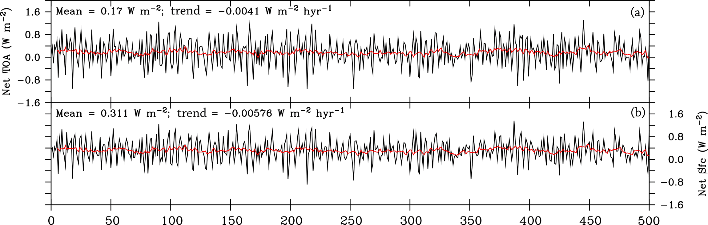
Figure 2Radiative energy balances in NESM v3. Time series of the net radiative energy fluxes at TOA (downward, W m−2, a) and the net heat flux at the Earth surface (W m−2, b) from year 0 to 500 in the preindustrial control experiment. The long-term mean value and trend are indicated in the upper left corner. The black lines indicate annual mean values and the red lines indicate their 9-year running mean values.
One of the major purposes of the PI control experiment is to verify the model's stability in the perpetual, unchanged forcing conditions. In this section, emphasis will put on evaluation of the equilibrium state of the top-of-atmosphere (TOA) atmosphere–ocean–sea ice interface to reveal the energy, water, and mass conservation of the whole system. The energy input at the TOA is the major energy source for the Earth system. It is vital to minimize the net energy imbalance at the TOA and surface, which can mitigate temperature drift in the system. At the air–sea interface, the major indicators are the land surface temperature and ocean surface temperature; they also work as a direct monitor of system energy conservation. Precipitation is the most important part of the global hydrological cycle, which involves energy exchange and mass exchange among the climate system components. Ocean salinity is sensitive to the state of the surface hydrological cycle, land runoff, and sea ice melting–formation process. Sea ice extent is a good indicator of sea ice amount in both the Arctic and Antarctic regions, and it is sensitive to ocean heat content drift and high-latitude energy transfer. To better quantify the climate drifts, linear trends were calculated for all evaluation variables.
The time evolution of the global mean energy budget at the TOA, Earth surface, and ocean surface is shown in Fig. 2. The global mean net shortwave radiation at the TOA averaged over the 500-year integration is 238.55 W m−2 and the corresponding outgoing longwave radiation (OLR) is −238.39 W m−2, resulting in a net atmospheric energy gain of 0.17 W m−2. The net heat budget at the TOA shows a negligible decreasing trend of −0.0041 W m−2 (100 yr)−1. At the Earth surface, the net energy imbalance is 0.31 W m−2 in the whole integration period with an insignificant decreasing trend of −0.00576 W m−2 (100 yr)−1. The negative trends are shown at both the TOA and surface, indicating the coupled system could lead to a more stable state when the integration extends. Note that there is a difference of 0.14 W m−2 between the surface and TOA net energy budget, which means the model atmosphere produces artificial energy. This problem is found also in the AMIP experiment and is probably due to the energy nonconservation in the model dynamical core.
The trends in the surface temperature indices, namely global mean surface air temperature, land surface temperature, and SST, reveal the energy conservation and stability as well as the stability of the sea, sea ice, air interaction in the coupled system (Fig. 3). The mean value of the near-surface air temperature (TAS) is 14.9 ∘C in the entire period, and the linear trend of TAS is 0.00214 ∘C (100 yr)−1. This trend is mainly attributed to the land surface temperature rather than SST. The linear trend of land surface temperature is −0.00984 ∘C (100 yr)−1. The slow balance of terrestrial (land) vegetation may be one of the reasons. The global time mean SST is 17.7 ∘C, which is consistent with the observation measured during the decade of 1870–1880. The negligible SST trend (0.00731 ∘C (100 yr)−1) indicates the global mean SST reached a quasi-equilibrium state. As the most important component of the global hydrological cycle, global mean precipitation has nearly no trend (Fig. 3). It is of interest that the global mean SST exhibits a long-term variability with a period of 50–100 years in this simulation. Possible mechanism and processes causing this variability will be discussed in a follow-up study.
To further verify the stability of the ocean component model, more variables are represented in Fig. 4. At the beginning of the PI experiment (coupled model spin-up), the sea surface salinity (SSS) has a quick adjustment process. The global mean SSS is decreased from 34.6 to 34.2 psu in 30 years. After the spin-up, the mean value of SSS is 34.2 psu, which is 0.5 psu fresher than the observed value. The long-term trend of SSS is −0.0077 psu (100 yr)−1, which indicates the ocean water flux is maintained at a relatively stable state. Meanwhile, the global mean sea water salinity (SWS) is 34.7 psu with a linear trend of −0.0038 psu (100 yr)−1. The total sea water temperature has an increasing trend of 0.032 ∘C (100 yr)−1, which is consistent with the surface energy budget showing a 0.43 W m−2 heating at the ocean surface. Furthermore, the linear trend in the last 100 years is smaller than the first 100 years. The decrease in the linear trend implies the model becomes more and more stable during the integration.
The Atlantic Meridional Overturning Circulation (AMOC) is a major source of decadal and multidecadal variability in the Earth system and influences the Arctic sea ice extent variability over the Atlantic sector (Mahajan et al., 2011). A time series of the maximum strength of the AMOC at 26.5∘ N is evaluated. The mean strength of the AMOC is 14.8 sv, which is underestimated compared to the modern observational value of 18.5 sv (Cunningham et al., 2007). The AMOC strength has a small linear trend and significant multidecadal variability.
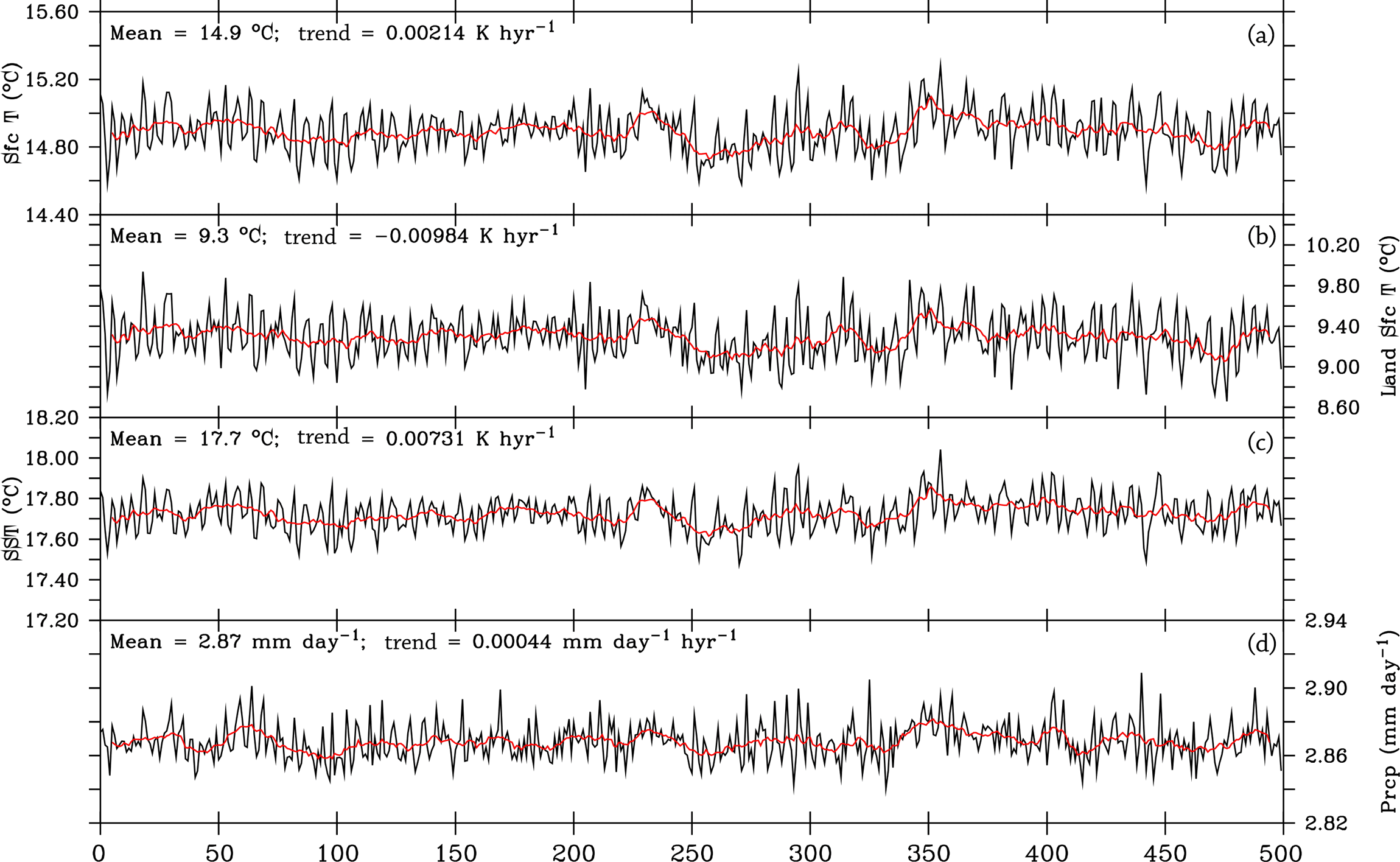
Figure 3Results from the preindustrial control experiment. Annual mean time series of surface temperature and precipitation from year 0 to 500 in the preindustrial control experiment; from top: near-surface air temperature (∘C), land surface temperature (∘C), sea surface temperature (∘C), and precipitation (mm day−1). The long-term mean value and trend are indicated in the upper left corners. The black lines are annual mean values and the red lines are their 9-year running mean values.
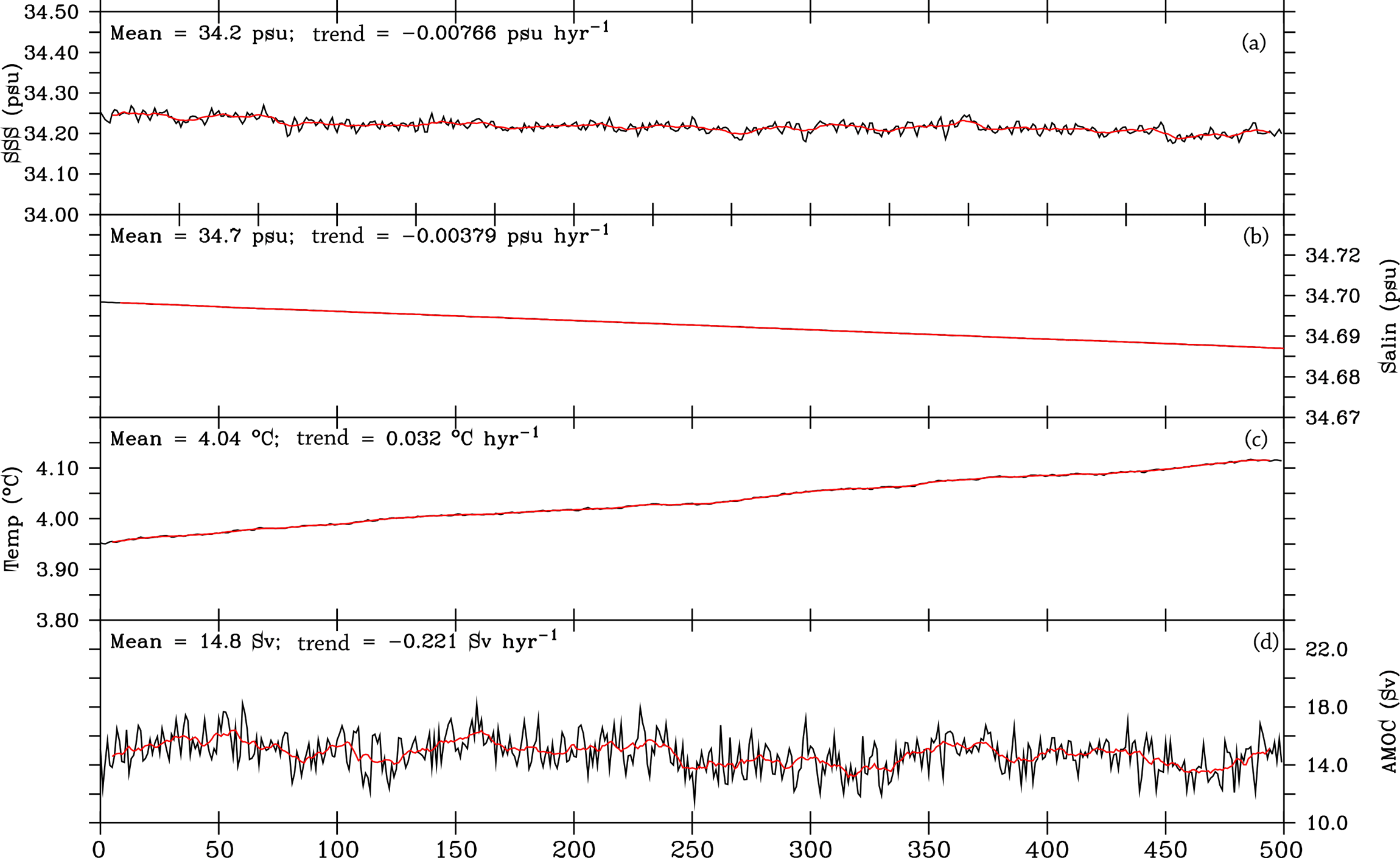
Figure 4Results from the preindustrial control experiment. Annual mean time series of the ocean variables from year 0 to 500; from top: sea surface salinity (psu), sea water salinity (psu), sea water temperature (∘C), and AMOC strength at 26.5∘ N (sv). The sea water salinity and sea water temperature are the volume mean values for the full-depth global ocean. The long-term mean value and trend are indicated in the upper left corner. The black lines are annual mean values and the red lines are their 9-year running mean values.
Table 1Summary of the global averaged annual mean values for radiation, temperature, and precipitation compared to observations. The observed energy estimations are from CERES ed2.8 for the period 2001–2014. The observed SST and LST data are derived from Hadley SST and CRU for the period 1870–1880 and 1901–1910, respectively. The combined CMAP and GPCP precipitation.
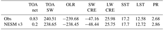
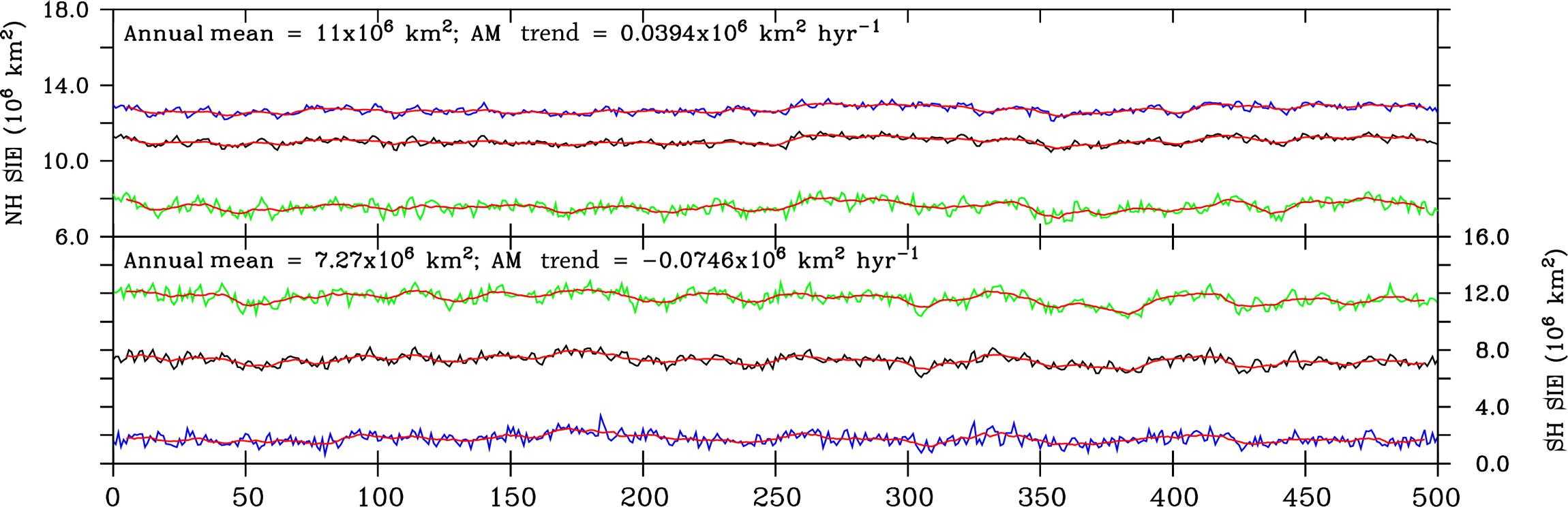
Figure 5Results from the preindustrial control experiment. The Northern Hemisphere (NH) and Southern Hemisphere (SH) sea ice extent (SIE; unit: 106 km2) time series from year 0 to 500 in the preindustrial control experiment. The black, blue, and green lines represent the annual mean, February, and September SIEs, and the red lines are the corresponding 9-year running mean. The long-term trends in annual mean SIEs are indicated in the upper left corner of each panel.
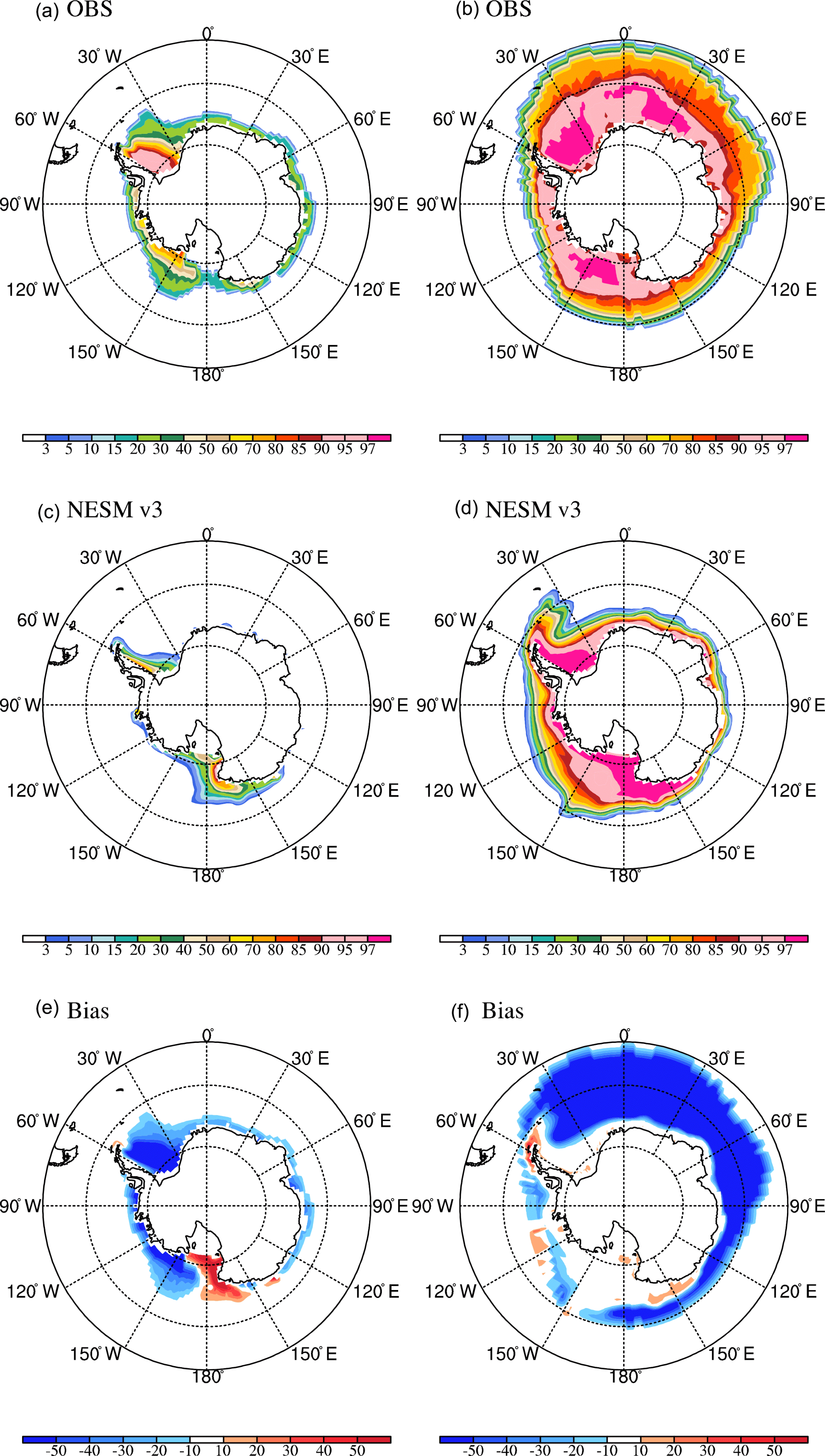
The middle and high-latitude climate, as well as the AMOC, is largely affected by sea ice state and its variability. Following the IPCC report, the February, September, and annual mean of Northern and Southern Hemisphere sea ice extents (SIEs) are diagnosed for the entire PI experiment period. The time evolutions of SIEs are plotted in Fig. 5. In the Northern Hemisphere (NH), the annual mean, February, and September mean SIE are 11×106, 12.7×10⁶, and 7.58×10⁶ km2, respectively. The trends of SIE over the NH in the annual mean, February, and September mean SIE are 0.039×10⁶, 0.06×10⁶, and 0.02×10⁶ km2 (100 yr)−1, respectively. These trends are small, suggesting that the Arctic SIE maintains a steady state. Over the SH, on the other hand, the trends in the annual mean, February, and September mean SIE are , , and km2 (100 yr)−1, respectively. This indicates that a significant trend exits in SH September only. The annual mean, February, and September mean SIEs are 7.27×10⁶, 1.73×10⁶, and 11.7×10⁶ km2, respectively. The bias of the SH sea ice extent is related to the extensive solar radiation over the Southern Ocean although the model overestimated cloud cover there (figure not shown). This is in part due to the thinner cloud optical depth in the simulated low-level cloud and shallow mixed layer depth over the Southern Ocean (Sterl et al., 2012).
The climatological mean states of some key fields for energy and water balance obtained from the average results for the last 100 years of the PI control run are compared with observations, including TOA energy fluxes, SST, land surface temperature, precipitation, atmospheric zonal mean zonal wind, temperature and specific humidity, and sea surface salinity. The observed energy flux data cover the period 2001–2014 and the observed SST is averaged over the period 1870–1880. The observational estimate of the land surface temperature is based on the 1901–1910 mean of CRU-TS-v3.22. The rest of the mean states are derived for the period 1979–2008.
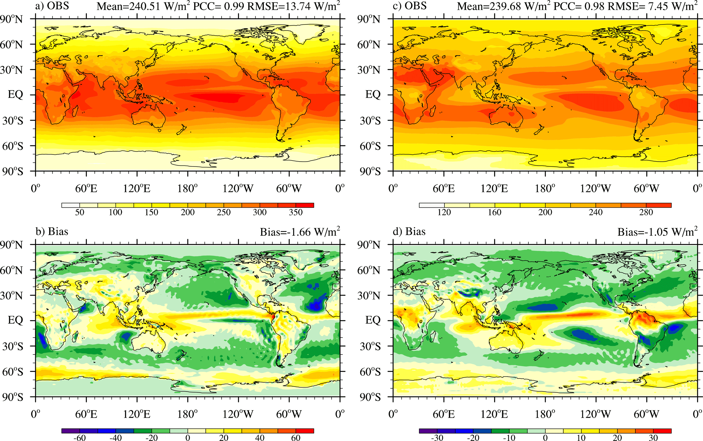
Figure 6Annual mean TOA net shortwave radiation (a, b) and OLR (c, d; unit: W m−2) derived from observations (a, c) and the model bias (b, d). The observed radiation fields were derived from the Clouds and the Earth's Radiant Energy System (CERES) dataset (Loeb et al., 2009).
The observed annual mean net shortwave (SW) radiation and OLR at the TOA and the model bias are shown in Fig. 6. The simulated global mean net solar radiation is 238.65 W m−2, which is smaller than the observation from CERES-EBAF data (Table 1). The model bias indicates excessive SW absorption over the ITCZ region and the Southern Ocean and less SW reflection over the middle-latitude oceans, which implies the planetary albedo is too high (Fig. 6b). Figure 6c shows the outgoing longwave radiation (OLR), which is balanced by the TOA net downward solar radiation and represents the atmospheric and cloud top temperature distribution. The global mean OLR is −238.45 W m−2 in the model, which is close to the counterpart from the CERES data and the differences are within the range of uncertainty among different observations (Loeb et al., 2009). The model simulates the vigorous deep-convection-related low OLR well over the Indo-Pacific warm pool and the high OLR in the desert and subtropical regions. However, the model overestimates the OLR over the majority of the ITCZ, the Indo-Pacific warm pool regions, and off the South American coast in the South Pacific. The model also underestimates the OLR in the North Atlantic storm track and western part of the Pacific subtropical high regions. These biases arise primarily from errors in simulated cloud fields.
The cloud radiative effect is defined as the difference between clear-sky and full-sky radiation. It indicates how cloud affects the radiation budget at the TOA. The simulated SW and LW cloud radiative effects (CREs) are compared with the CERES-EBAF ed2.8 in Fig. 7. NESM v3 simulates a global averaged annual mean SW CRE of −48.4 W m−2 compared to the observed value of −47.2 W m−2. The simulated LW CRE is 25.98 W m−2, which is close to the observed value of 25.75 W m−2. The total cloud radiative effect in the NESM v3 is −22.5 W m−2, which is comparable with the CERES-EBAF observation (−21.45 W m−2). The bias pattern of SW CRE is similar to that of the net SW radiation at TOA. The model produces positive SW CRE over the tropics although the simulated cloud cover bias is small (figure not shown). This suggests the importance of cloud vertical distribution and cloud properties in determining the CRE. In addition, the LW CRE bias is smaller than the SW CRE, indicating the model has a better representation of high cloud.
The climatological mean SST and land surface temperature (LST) are compared with the observational data in Fig. 8. SST is one of the most important variables in the coupled system, which reflects the quality of the model's simulation of atmosphere–ocean interaction processes. The model captures the global distribution of SST well with a warm pool in the Indo-Pacific region and the cold tongue over the eastern Pacific. There are warmer biases in the Southern Ocean and off the western coasts of America and Africa (Fig. 8b), which is linked to the excessive downward shortwave radiation induced by the negative bias in simulated stratiform clouds. Significant cold SST biases are found in the high-latitude North Atlantic around 50∘ N with a maximum negative bias of −4 K. Cold biases are also seen in the subtropical North Pacific and North Atlantic.
The land surface temperature is shown in comparison with CRU-TS-v3.22 (1901–1910). The model reproduces the basic patterns of the LST well, including warm continents in equatorial regions and cold continents close to polar regions. The simulated global averaged (70∘ S–90∘ N) LST is 12.72 ∘C, which is slightly warmer than the observed value of 12.58 ∘C (Table 1). The warm temperature bias is mainly found over central Asia, Canada, and Australia (Fig. 8d).
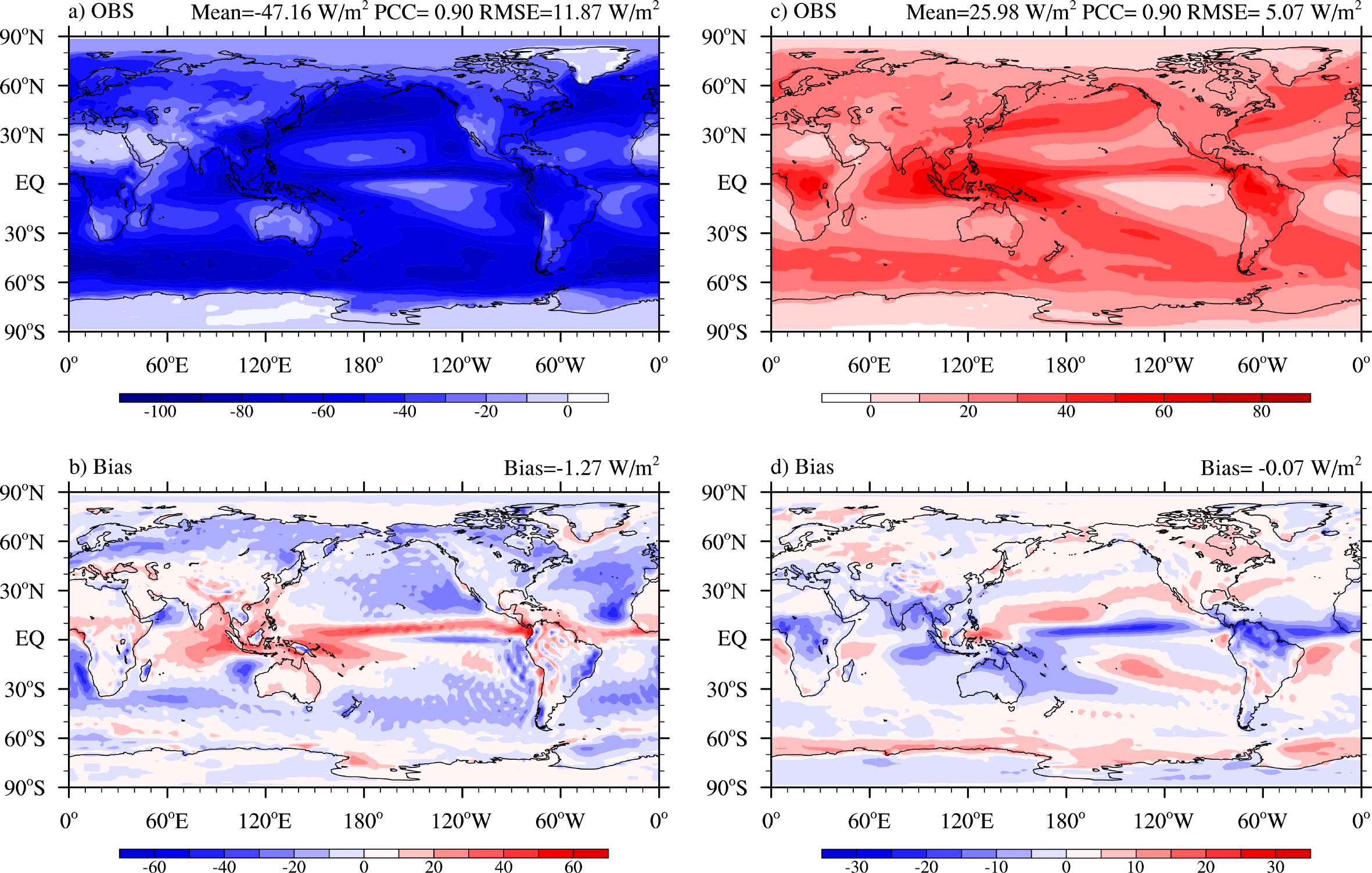
Figure 7Annual mean TOA shortwave (a, b) and longwave (c, d) cloud radiative effect (c, d; unit: W m−2) derived from observations (a, c) and the model bias (b, d). The observed radiation fields were derived from the Clouds and the Earth's Radiant Energy System (CERES) dataset (Loeb et al., 2009).
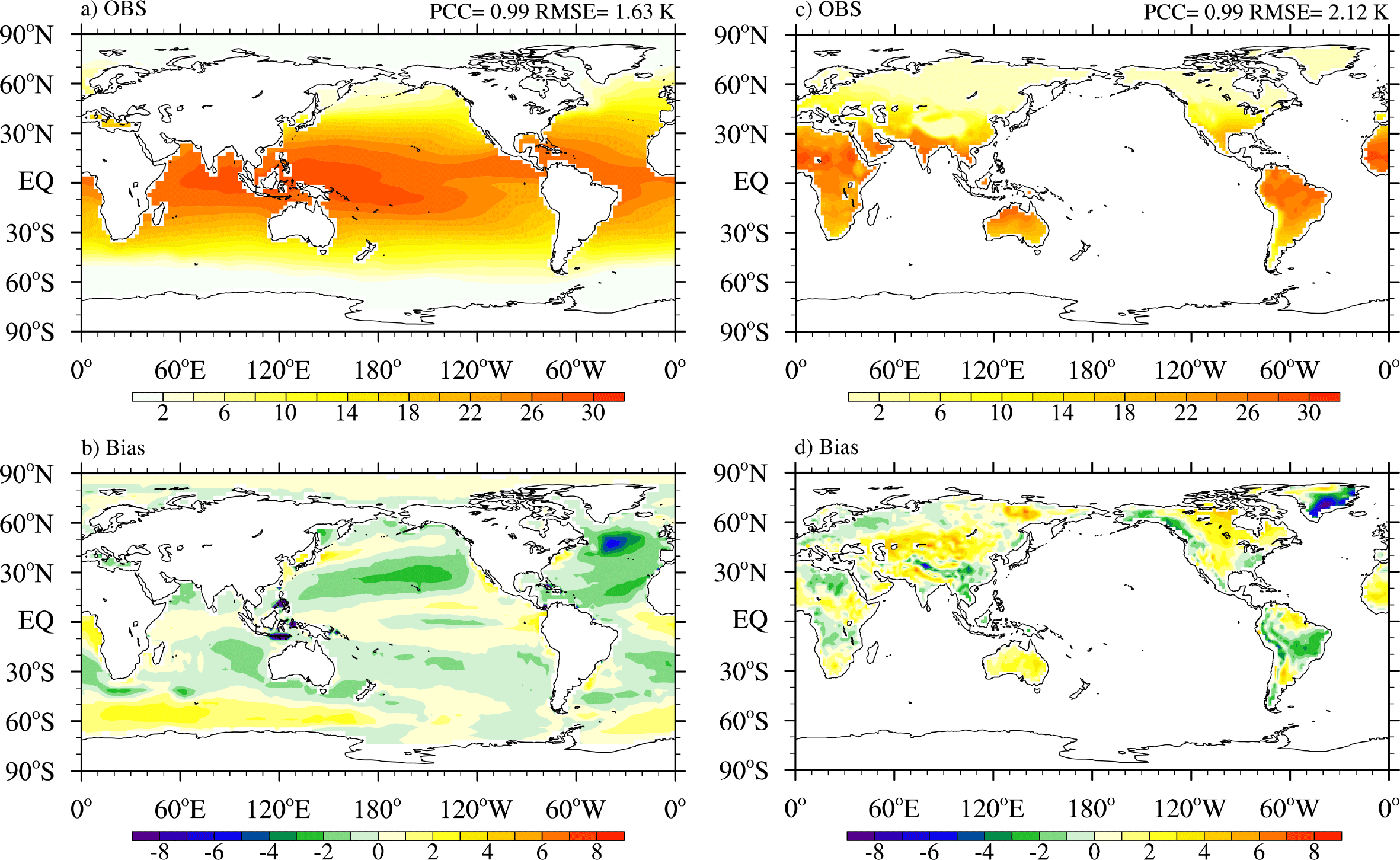
Figure 8The annual mean SST (a, b) and land surface temperature (c, d, ∘C) derived from observations (a, c) and the model bias (b, d). The observed SST climatology was derived from the Hadley Centre Sea Ice and Sea Surface Temperature (HadISST; Rayner et al., 2003) for the period 1870–1880. The observed land surface climatology was derived from the CRU-TS-v3.22 (Harris et al., 2014) for the period 1901–1910.
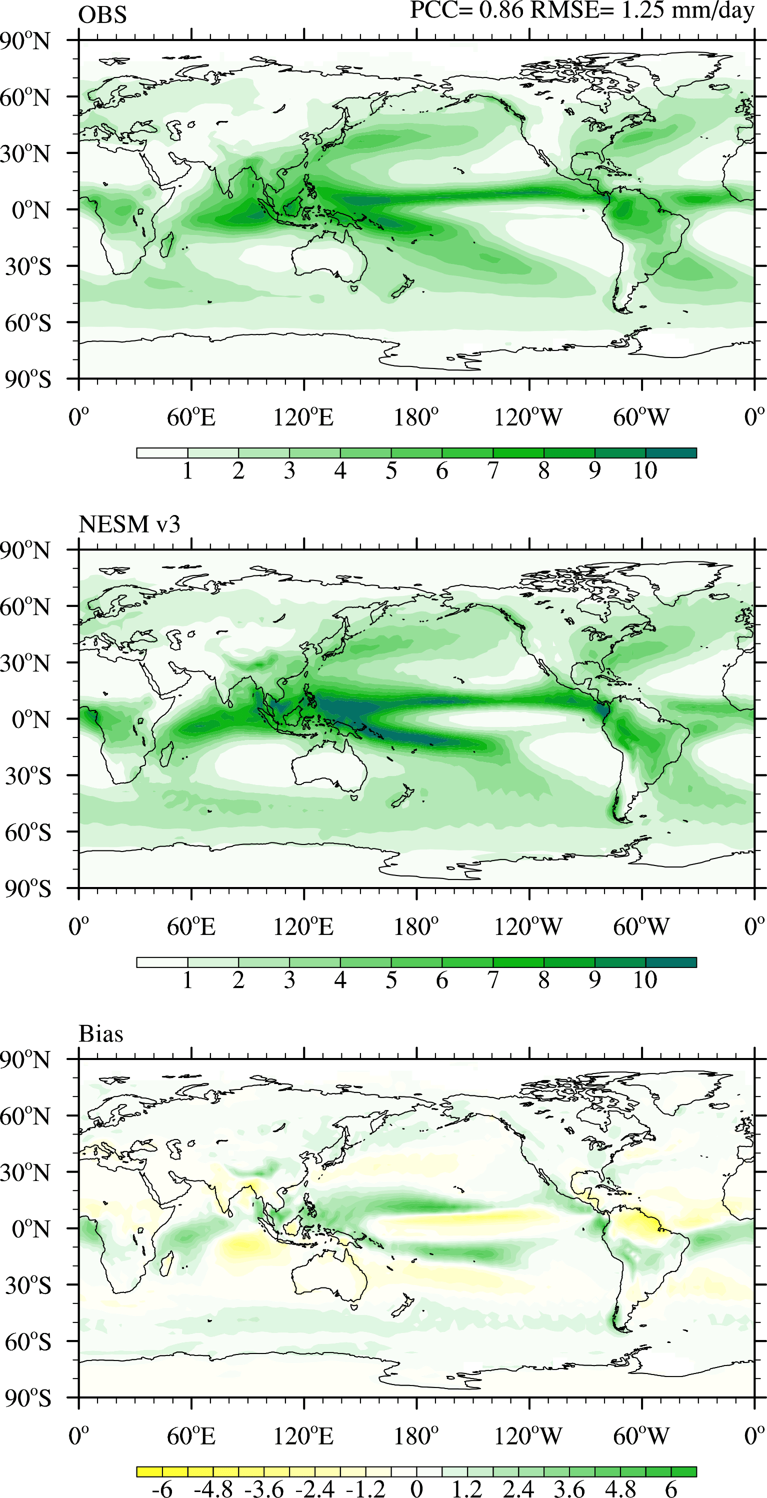
Figure 9The climatological mean precipitation (mm day−1) in observations, NESM v3, and model bias. The observed precipitation was derived from a merged precipitation dataset (Lee and Wang, 2014), which is the arithmetic mean of the monthly data from the Global Precipitation Climatology Project (GPCP) version 2.2 (Adler et al., 2003) and Climate Prediction Center Merged Analysis of Precipitation (CMAP; Xie and Arkin, 1997).
Figure 9 compares the spatial pattern of observed and simulated precipitation. The simulated precipitation pattern and intensity resemble the observations (pattern correlation coefficient, PCC=0.86), which capture the observed rain bands over the ITCZ, South Pacific Convergence Zone (SPCZ), tropical Indian Ocean, and the midlatitude storm-track regions. However, the so-called double ITCZ precipitation bias exists in the Pacific Ocean and Atlantic Ocean, which is partially linked to simulated TOA shortwave radiation bias (Xiang et al., 2017) and insufficient stratocumulus clouds over the eastern Pacific (Bacmeister et al., 2006; Song and Zhang, 2009). The precipitation bias shows a dipole pattern over the tropical Indian Ocean. From an atmospheric point of view, such a model deficiency is mainly attributed to the SST bias over the tropics, but it is essentially a coupled model bias.
The zonal mean climatological temperature, zonal wind, and specific humidity along with their biases with respect to ERA-Interim are presented in Fig. 10. Overall, the model captures the temperature, zonal wind, and specific humidity distribution reasonably well. The temperature and zonal wind biases are small over a majority of the region. However, there are 6 K cold biases at 200 hPa over high latitudes in both hemispheres (Fig. 10b). The biases increase the tropics-to-pole temperature gradient in the upper troposphere, which produces an enhanced subtropical jet. The westerly wind bias is about 6 m s−1 in the subtropical jet of both hemispheres and over the Equator in the upper troposphere (Fig. 10d). The model simulated less water vapor within the boundary layer, while it overestimated the specific humidity above the boundary layer (Fig. 10f).
The sea surface salinity (SSS) is an integrated indicator for the hydrological interaction among ocean, atmosphere, land runoff, and sea ice, as well as ocean circulation. Accurate simulation of ocean circulation in climate models is essential for correct estimation of the transient ocean heat uptake and climate response, sea level rise, and coupled modes of climate variability. Figure 11 shows the observed climatological SSS and the model bias. In general, the model realistically simulates the high SSS over the subtropics, where precipitation is low and evaporation is high, and the relatively low SSS over the ITCZ region where precipitation is heavy. The global mean SSS has a negative bias of 0.5 psu, which is mainly due to the fresh bias over the North Atlantic and the western equatorial Pacific. Over the western equatorial Pacific, extensive precipitation is the major cause. Over the North Atlantic, the excessive net input of fresh water is a primary cause, which is augmented by weak evaporation at high latitudes. The freshwater bias in the North Atlantic can also be attributed to the bias in simulated North Atlantic currents and excessive sea ice melt over the Labrador Sea. Previous studies pointed out that the freshwater bias over the high latitudes of North Atlantic can weaken ocean convection so that the AMOC is weakened (Rahmstorf, 1995).
The simulated February and September sea ice concentrations in both hemispheres are compared with observations in the period 1870–1880 (Figs. 12 and 13). In the NH, the spatial distribution of the summer and winter sea ice concentration is well captured by the NESM v3. Over the Southern Hemisphere, the model significantly underestimates sea ice concentration, especially during austral summer. As discussed in the previous section, there is an extensive solar radiation bias over the Southern Ocean that leads to a warm SST bias, especially during local summer when solar radiation is high.
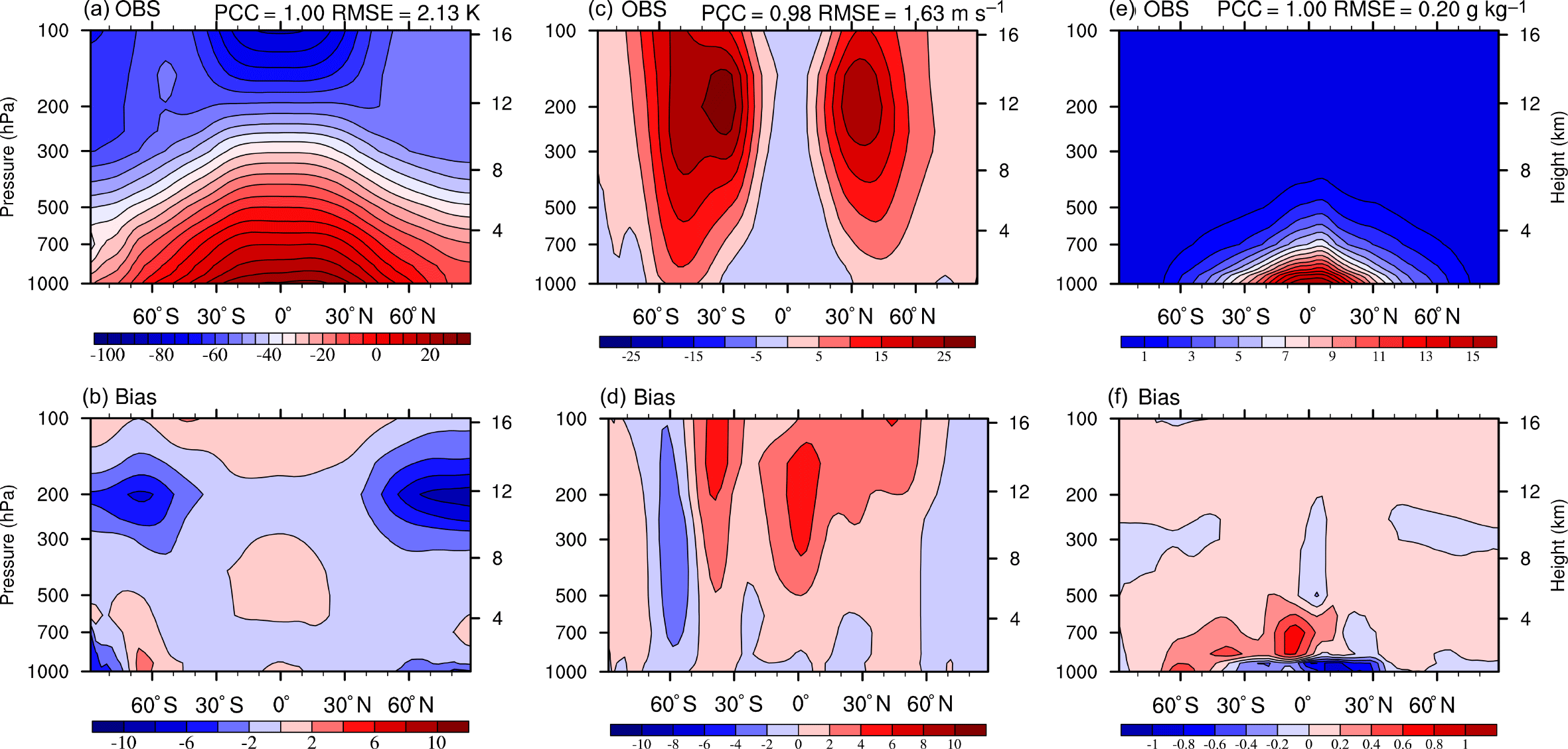
Figure 10The zonal and climatological mean of temperature (a, b; K), zonal wind (c, d; m s−1), and specific humidity (e, f; g kg−1) in observations (a, c, e) and model bias (b, d, f). The observational data were derived from ERA-Interim (1979–2008).
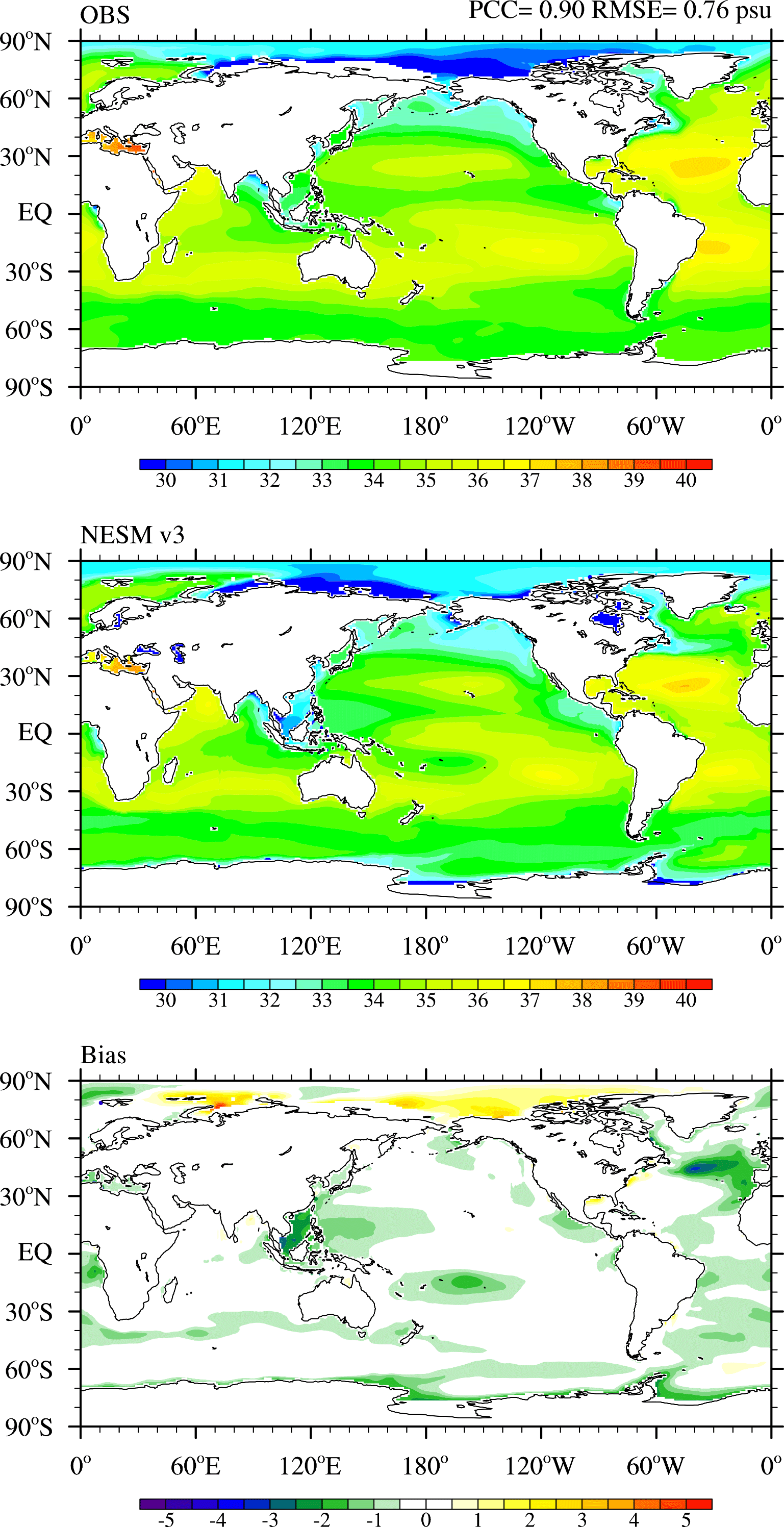
Figure 11Same as in Fig. 9 except for the annual mean sea surface salinity (psu). The observed SSS data are from the World Ocean Atlas 2009 (WOA09; Locarnini et al., 2010).
Quantification of climate response to different forcing and estimation of the associated radiative forcing can benefit from sensitive experiments with a single perturbation forcing, such as an abruptly quadrupling CO2 (abrupt4xCO2) simulation and a 1 % yr−1 CO2 increase (1pctCO2) experiment. Following the CMIP6 protocols, the two CO2 experiments are designed to document basic aspects of the NESM v3 response to greenhouse gas forcing. They are both branched from the PI simulation and the only difference is the imposed CO2 concentrations. In the abrupt4xCO2 experiment, the atmospheric CO2 concentration is abruptly quadrupled (1139 ppm) with respect to the PI condition (274.75 ppm) in the very beginning of the experiment. The 1pctCO2 is designed as gradually increasing the CO2 concentration at the rate of 1 % per year. Both experiments were initiated at the end of year 100 of the PI experiments, and each of them was integrated for 150 years.
Figure 14 shows the global annual mean surface air temperature (TAS) changes with respect to its mean value in the PI experiment. Once the atmospheric CO2 is instantaneously quadrupled, the radiative forcing defined by the net downward heat flux induced by the changing atmospheric carbon dioxide concentration forces the stratospheric and tropospheric circulations to adjust, thereby changing the surface temperature. The TAS rapidly increases by approximately 4.5 K in the first 20 years in response to the imposed radiative forcing. After the rapid initial increase, the TAS gradually increases, mitigating the energy imbalance at the TOA.
The abrupt4xCO2 experiment is used not only to diagnose the fast response of the Earth system, but also to quantify the radiative forcing and to estimate the equilibrium climate sensitivity (ECS). The ECS is regarded as the global equilibrium TAS change in response to the doubling atmospheric carbon dioxide concentration. It is also indicated by the ratio of the radiative forcing to the climate feedback parameter. The regression of TOA energy imbalance and global mean TAS change is an effective method to obtain those estimations (Gregory et al., 2004) since it does not require the equilibrium state of GCM. The intersection of the regression line and the y axis is recognized as the adjusted radiative forcing, and the intersection on the x axis is an indication of the equilibrium temperature. The slope of the regression line is the climate feedback parameter.
The relationship between the change in the net TOA energy imbalance and global mean TAS change is plotted in Fig. 15. It shows that the TOA radiative imbalance is around 7.24 W m−2 when the assumed global TAS is unchanged, although the radiative forcing is affected by the rapid adjustments of the stratosphere in the first year and therefore reduces the effective radiative forcing (Gregory and Webb, 2008). To balance the net TOA energy, the regression predicted an equilibrium temperature change of 7.38 K in this model, which yields a climate feedback parameter of −0.98 W m−2 K−1. Since the radiative forcing is logarithmically related to the carbon dioxide concentration if we approximate the climate feedback parameter as a constant (Hansen et al., 2005a, b), this gives an ECS of 3.69 K. Andrews et al. (2012) found that the CMIP5 ensemble mean of regressed 4×CO2 adjusted forcing is 6.89±1.12 W m−2 and the climate feedback parameter is W m−2 K−1, with an ECS of 3.37±0.29 K. The carbon-dioxide-induced radiative forcing and climate feedback parameter estimated by NESM v3 are comparable with the CMIP5 ensemble, although the estimated ECS is about 10 % higher.
The climate sensitivity parameter consists of longwave clear-sky, shortwave clear-sky, longwave cloud forcing, and shortwave cloud forcing terms. They are defined by the heat flux differences between the abrupt4xCO2 experiment and PI experiment. The sum of the longwave cloud forcing and shortwave cloud forcing is the total CRE. Here the downward fluxes are defined as positive. Figure 16 shows the relationships between the changes in the global mean heat fluxes and the change in the surface air temperature. The longwave clear-sky feedback strength is −1.63W m−2 K−1, which is partially offset by the shortwave clear-sky feedback (0.68 W m−2 K−1), resulting in a residual feedback strength of −0.95 W m−2 K−1, which is close to the climate sensitivity parameter estimated in this model (−0.98 W m−2 K−1). The slopes of the shortwave and longwave cloud forcing have nearly the same magnitude but with opposite signs, yielding a small positive cloud radiative effect (0.02 W m−2 K−1) in this model. It could be the reason for the slightly high ECS in NESM v3 since the CMIP5 results suggested that the GCM with higher sensitivity is associated with a positive CRE feedback (Andrews et al., 2012). And the CRE is a major contributor to the uncertainty in the climate sensitivity parameter in CMIP3 and CMIP5, although its magnitude is small compared to other flux terms (Webb et al., 2006; Andrews et al., 2012).
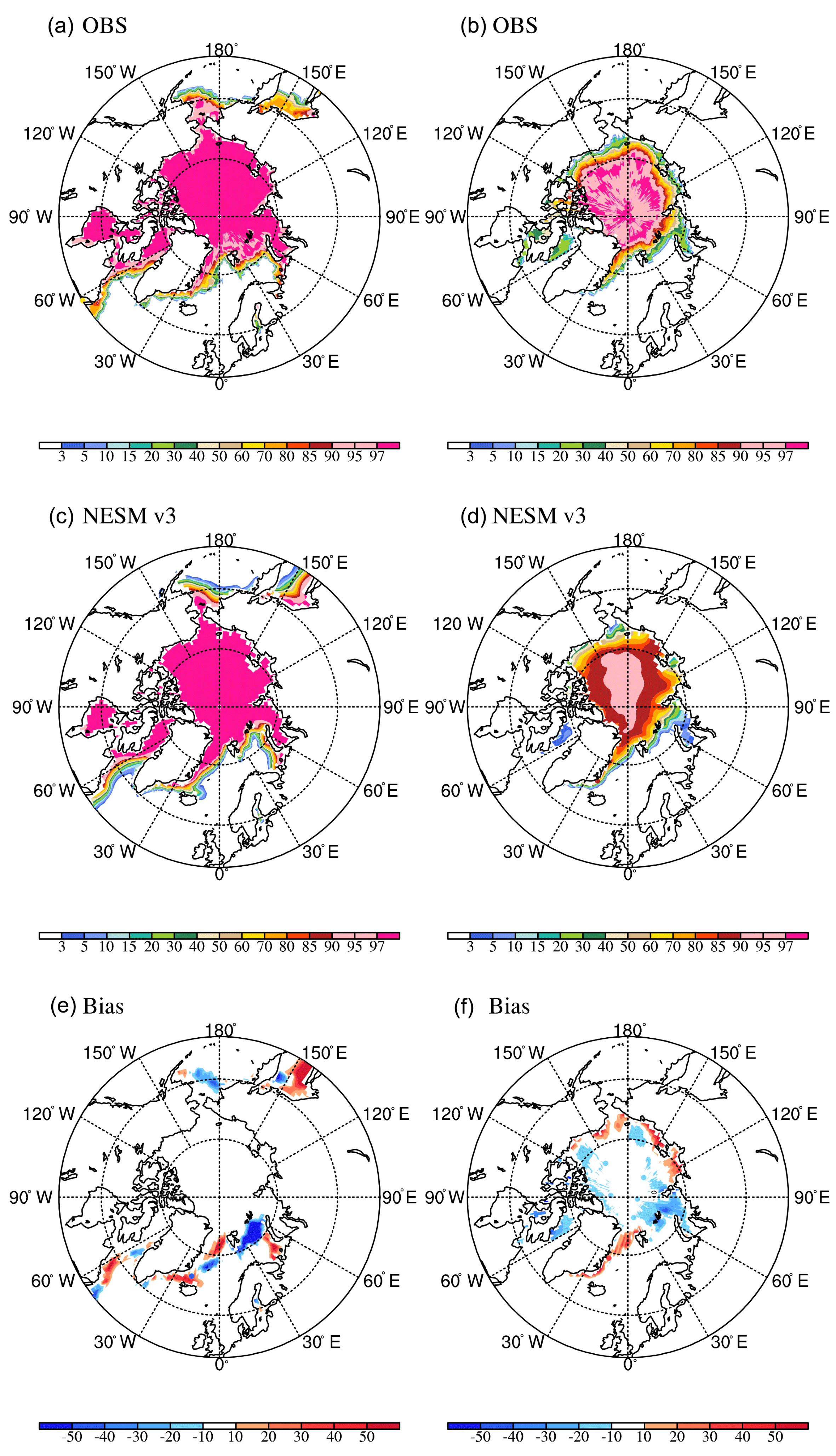
Figure 12Climatological Arctic sea ice concentration in HadISST (a, b), NESM v3 (c, d), and model bias (e, f) for February (a, c, e) and September (b, d, f). The observed sea ice concentration is averaged over the period 1870–1880.
Figure 17 displays the global distributions of temperature and precipitation in response to the quadruple CO2 forcing, which are defined by the departure of the last 30-year climatology from the corresponding climatology in the PI experiment. The most pronounced warming is seen over the Arctic region where sea ice albedo feedback dominates (Screen and Simmonds, 2010). The relative small temperature change is over the Southern Ocean and North Atlantic. The warming is more significant over land than ocean, especially in the Northern Hemisphere. The mean surface temperatures over land and ocean are 8.0 and 5.2 K, respectively. The equatorial Pacific shows an El Niño-like warming. The zonal mean surface temperature change shows an obvious polar amplification, especially over the Arctic Ocean, stronger warming over the NH high latitudes, and weak warming in the SH middle latitudes. The large NH temperature increase is attributed to the strong warming over the Arctic Ocean and the large land area in the NH.
A direct consequence of global warming is the rising atmospheric specific humidity and precipitation. The global mean precipitation has increased from 2.87 to 3.12 mm day−1, resulting in a precipitation increase of 1.4 % per Kelvin global warming. Significant precipitation increases are seen in the equatorial Pacific and northern Indian Ocean as well as along the Pacific storm track (Fig. 17). Decreased precipitation is evident in the subtropical descent zones. Note that precipitation is decreased over the Amazon region, where the model has a dry bias in climatology. The global distribution of precipitation change appears to be dominated by the wet-get-wetter pattern (Held and Soden, 2006).

Figure 14Results from the abrupt quadrupling of CO2 experiment. Global mean surface air temperature change relative to the counterpart in the PI experiment.
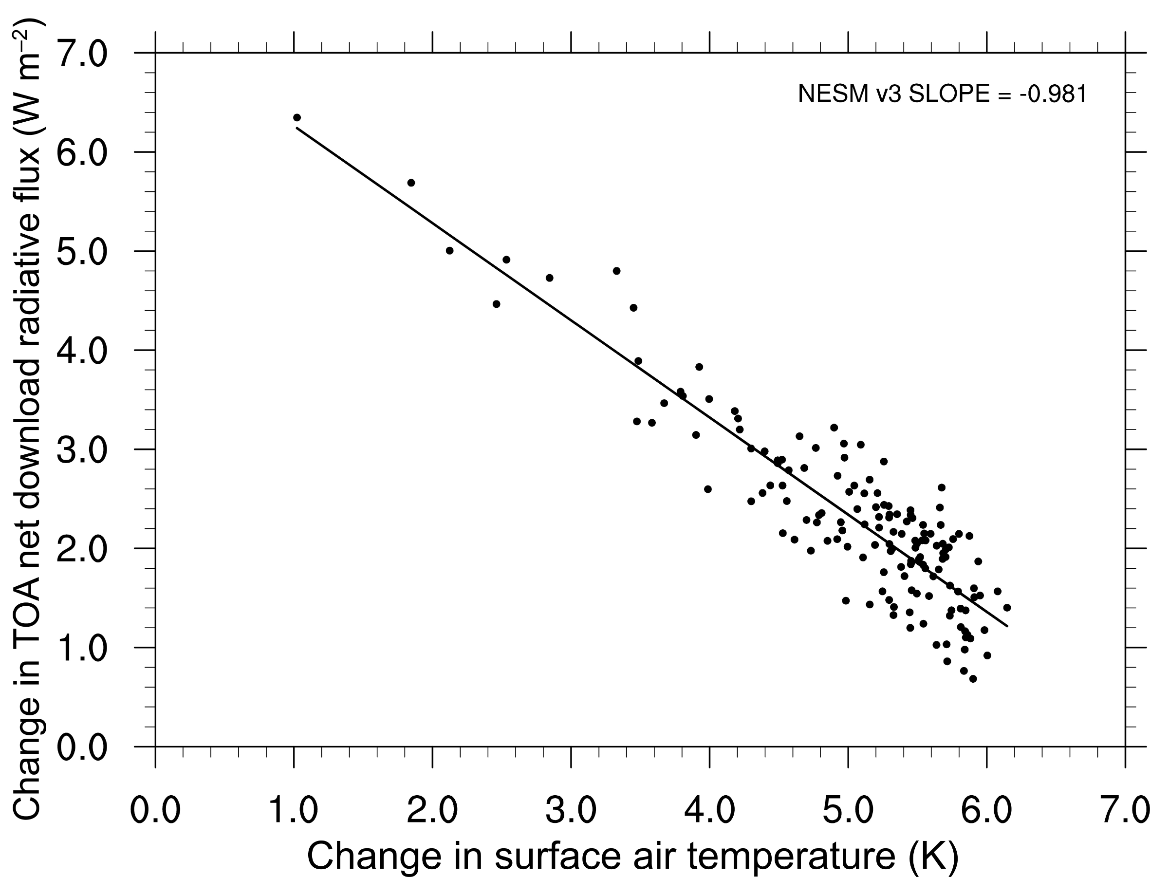
Figure 15Results from the abrupt quadrupling of CO2 experiment. The relationships between the change in the net TOA radiative flux and the global mean surface air temperature in NESM v3. The solid line represents a linear least squares regression fit to the 150 years of model output data. The interception at δT=0 indicates the adjusted radiative forcing (F=7.24 W m−2). The slope of the regression line measures the strength of the feedbacks in the climate system, which is the climate feedback parameter (−0.981 W m−2 K−1). The interception at the x axis gives the equilibrium δT (7.38 K).
In reality, the CO2 increase is gradual rather than abrupt. The 1pctCO2 experiment is designed to examine the transient climate response (TCR), which is calculated by using the global mean TAS change between the averaged 20-year period centered at the timing of CO2 doubling (years 60–80 in the 1pctCO2 experiment) and the PI experiment. The time evolution of the global mean TAS anomalies with respect to the PI experiment is shown in Fig. 18. A linear increase in temperature anomalies is presented in the gradual CO2-increasing experiment. The temperature anomalies averaged between year 60 and 80 are 2.16 K. This value of TCR is significantly smaller than the ECS, demonstrating that the ocean heat uptake delays surface warming. The estimation from CMIP5 shows that the mean TCR is 1.8±0.6 K (Flato et al., 2013), implying that NESM v3 is comparable to other CGCMs.
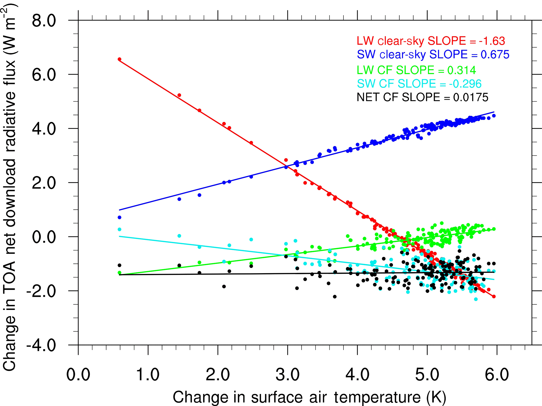
Figure 16Results from the abrupt quadrupling of CO2 experiment. The relationship between the change in the global mean radiative fluxes and global mean surface air temperature. The climate feedback parameters (W m−2 K−1) for the TOA longwave clear-sky (red), shortwave clear-sky (green), longwave cloud forcing (blue), shortwave cloud forcing (light blue), and net cloud radiative effect (black) are −1.63, 0.675, 0.31, −0.30, and 0.02 W m−2 K−1, respectively.

Figure 17Changes in the surface temperature (a) and precipitation (b) derived from the last 30-year climatology in the 150-year abrupt4xCO2 experiments. The changes are with reference to the corresponding climatological mean fields from the PI experiment. The right panels show the corresponding zonal mean changes.
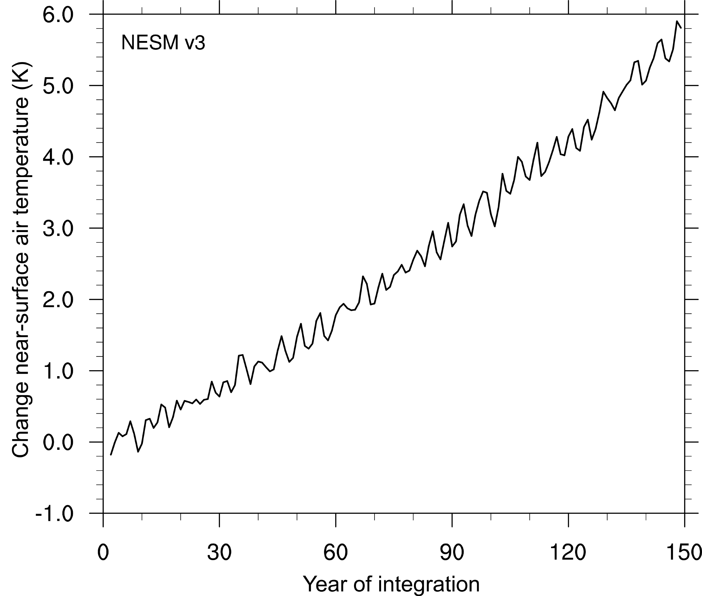
Figure 18Results from the 1 % per year CO2 increase experiment. Global mean annual surface air temperature change relative to the counterpart in the PI experiment. The average temperature anomaly between years 60 and 80 is defined as transit climate sensitivity, which is 2.16 K in NESM v3.
The development of version 3 of the Nanjing University of Information Science and Technology (NUIST) Earth System Model (NESM v3) aims at building up a comprehensive numerical modeling laboratory for multidisciplinary studies of the climate system and Earth system. As a subsequent version of NESM v1, it has upgraded atmospheric and land surface models, increased ocean model resolution, improved coupling conservation, and modified model physics.
The NESM v3 couples the ECHAM v6.3 atmospheric model, JSBACH land surface model, NEMO v3.4 ocean model, and CICE v4.1 sea ice model by using the OASIS3-MCT_3.0 coupler. The improvement of model physics mainly focuses on convective parameterizations, cloud macrophysics and microphysics, and ocean–sea ice coupling. The model physics modifications and parameter adjustments are targeted at (1) obtaining stable long-term integrations and reasonable global mean states under the preindustrial (PI) forcing, (2) mitigating the biases in the mean climatology and internal modes of climate variability with respect to the modern observations in the present-day forcing condition, and (3) simulating reasonable climate responses to transient and abrupt CO2 forcing.
A 500-year PI experiment is conducted and analyzed to test the model's computational stability. As shown in Sect. 4, the long-term climate drifts in NESM v3 are generally negligibly small, especially in global radiative energy and temperature. The simulated net downward energy fluxes at the TOA and surface are 0.17 and 0.35 W m−2, respectively. The near-equilibrium model long-term temperature evolution benefits from the near-zero energy imbalance and negligibly small trends in the energy balance. The global mean near-surface air temperature is 14.9 ∘C with a trend of 0.00214 ∘C (100 yr)−1. The linear trends of the land surface and sea surface temperature are −0.00984 and 0.00731 ∘C (100 yr)−1, respectively. However, the total sea water temperature has a warming trend of 0.03 ∘C (100 yr)−1, which can be explained by the small but persistent positive downward energy flux into the ocean. The stable long-term evolutions of precipitation, sea surface salinity (SSS), and sea water salinity (SWS) demonstrate the conservation of global water. At the beginning of PI experiment spin-up, there was a freshening trend in SSS, which is associated with the ocean adjustment. The fresher SSS has no significant influence on SWS. After the spin-up, the global mean SSS and SWS have no appreciable trends although the SSS is fresher than the observed counterpart. The northern hemispheric annual mean, February, and September mean SIEs maintain a steady value at 11.4×10⁶, 13.4×10⁶, and 7.78×10⁶ km2, respectively. However, the simulated Southern Hemisphere SIEs are less than the present-day observation. The conservation properties of NESM v3 are encouraging, fulfilling a highly desirable constraint for climate models aiming for multidecadal, centennial, and longer simulations.
The last 100-year results are compared with the available observations as presented in Table 1. The TOA energy budget and cloud radiative effect have attracted more attention because of their importance in understanding the climate change. The model results show a realistic global climate, although the bias of energy state still exists, especially over the Indo-Pacific region, which may be related to the treatment of cloud and convection parameterization. The annual mean SST and LST are well produced in the model, but there are large cold biases in the North Atlantic, significant warm biases in the Southern Ocean, and a warm temperature bias over central Asia. The simulated mean precipitation is reasonably realistic, but suffers from the double ITCZ syndrome. The fresh bias in SSS in the tropical western North Pacific can be attributed to extensive precipitation, and the fresh bias over the midlatitude North Atlantic is related to underestimated evaporation. The sea ice coverage is well reproduced by the model over the Arctic in February and September; however, it is underestimated over the Antarctic where SST has a warm bias.
The model produces a radiative forcing under the abrupt quadrupling of carbon dioxide of 7.24 W m−2 with a climate feedback parameter of −0.98 W m−2 K−1, yielding a warming of 7.38 K at the estimated equilibrium state. The transient climate sensitivity is 2.16 K, which is estimated from the 1 % yr−1 CO2 gradually increasing experiment. NESM v3 is amongst the more sensitive of the CMIP5 class of global climate models.
This paper is not aimed at providing a comprehensive evaluation of all model aspects. Its response to given SST forcing in AMIP, the historical forcing in the coupled model, the corresponding modern climatology, internal and coupled modes of climate variability, and regional climate variability will be discussed in detail in a later accompanying paper.
Please contact Jian Cao (jianc@nuist.edu.cn) to obtain the source code and data for NESM v3.
BW designed the model's overall structure and the strategy for the development of the model. BW and JC led the modeling group work. JC, Y-MY, and LM were responsible for code development and model improvement. BW, JL, JH, BS, YB, and XZ were responsible for diagnosis of the model results. JC and BW drafted the original paper and LM, JL, YB, Y-MY, and LW contributed to revising the paper.
The authors declare that they have no conflict of interest.
This work is supported by the Nanjing University of Information Science and
Technology through funding from the joint China–US Atmosphere–Ocean Research
Center at the University of Hawaii. Jian Cao is thankful for the support of
the
National Key R & D Program of China (2017YFA0603801), and Jian Cao and Liguang Wu
are thankful for the support of public science and technology ocean research
project funds (201505013). The IPRC publication number is 1327
and the ESMC publication number is 225.
Edited by: Olivier Marti
Reviewed by: two anonymous referees
Adcroft, A., Hill, C., and Marshall, J.: Representation of topography by shaved cells in a height coordinate ocean model, Mon. Weather Rev., 125, 2293–2315, 1997.
Adler, R. F., Huffman, G. J., Chang, A., Ferraro, R., Xie, P., Janowiak, J., Rudolf, B., Schneider, U., Curtis, S., Bolvin, D., Gruber, A. Susskind, J., Arkin, P., and Nelkin, E.: The version 2 Global Precipitation Climatology Project (GPCP) monthly precipitation analysis (1979–present), J. Hydrometeorol., 4, 1147–1167, 2003.
Andrews, T., Gregory, J. M., Webb, M. J., and Taylor, K. E.: Forcing, feedbacks and climate sensitivity in CMIP5 coupled atmosphere-ocean climate models, Geophys. Res. Lett., 39, L09712, https://doi.org/10.1029/2012GL051607, 2012.
Bacmeister, J. T., Suarez, M. J., and Robertson, F. R.: Rain reevaporation, boundary layer–convection interactions, and Pacific rainfall patterns in an AGCM, J. Atmos. Sci., 63, 3383–3403, 2006.
Barnier, B., Madec, G., Penduff, T., Molines, J.-M., Treguier, A.-M., Sommer, J. L., Beckmann, A., Biastoch, A., Boning, C., Dengg, J., Derval, C., Durand, E., Gulev, S., Remy, E., Talandier, C., Theetten, S., Maltrud, M., McClean, J., and Cuevas, B. D.: Impact of partial steps and momentum advection schemes in a global ocean circulation model at eddy-permitting resolution, Ocean Dynam., 56, 543–567, 2006.
Beckmann, A. and Doscher, R.: A method for improved representation of dense water spreading over topography in geopotential-coordinate models, J. Phys. Oceanogr., 27, 581–591, 1997.
Brinkop, S. and Roeckner, E.: Sensitivity of a general circulation model to parameterizations of cloud-turbulence interactions in the atmospheric boundary layer, Tellus A, 47, 197–220, 1995.
Brovkin, V., Boysen, L., Raddatz, T., Gayler, V., Loew, A., and Claussen, M.: Evaluation of vegetation cover and landsurface albedo in MPI-ESM CMIP5 simulations, J. Adv. Model. Earth Syst., 5, 48–57, https://doi.org/10.1029/2012MS000169, 2013.
Cao, J. and Wu, L.: Asymmetric impact of last glacial maximum ice sheets on global monsoon activity, J. Meteorol. Sci., 36, 425–435, 2016.
Cao, J., Wang, B., Xiang, B., Li, J., Wu, T., Fu, X., Wu, L., and Min, J.: Major modes of short-term climate variability in the newly developed NUIST Earth System Model (NESM), Adv. Atmos. Sci., 32, 585–600, https://doi.org/10.1007/s00376-014-4200-6, 2015.
Cunningham, S. A., Kanzow, T., Rayner, D., Baringer, M. O., Johns, W. E., Marotzke, J., Longworth, H. R., Grant, E. M., Hirschi, J. J.-M., Beal, L. M., Meinen, C. S., and Bryden, H. L.: Temporal variability of the Atlantic Meridional Overturning Circulation at 26∘ N, Science, 317, 935–938, 2007.
Dee, D. P., Uppala, S. M., Simmons, A. J., Berrisford, P., Poli, P., Kobayashi, S., Andrae, U., Balmaseda, M. A., Balsamo, G., Bauer, P., Bechtold, P., Beljaars, A. C. M., van de Berg, L., Bidlot, J., Bormann, N., Delsol, C., Dragani, R., Fuentes, M., Geer, A. J., Haimberger, L., Healy, S. B., Hersbach, H., Hólm, E. V., Isaksen, L., Kållberg, P., Köhler, M., Matricardi, M., McNally, A. P., Monge-Sanz, B. M., Morcrette, J.-J., Park, B.-K., Peubey, C., de Rosnay, P., Tavolato, C., Thépaut, J.-N., and Vitart, F.: The ERA-Interim reanalysis: configuration and performance of the data assimilation system, Q. J. Roy. Meteorol. Soc., 137, 553–597, https://doi.org/10.1002/qj.828, 2011.
Eyring, V., Bony, S., Meehl, G. A., Senior, C. A., Stevens, B., Stouffer, R. J., and Taylor, K. E.: Overview of the Coupled Model Intercomparison Project Phase 6 (CMIP6) experimental design and organization, Geosci. Model Dev., 9, 1937–1958, https://doi.org/10.5194/gmd-9-1937-2016, 2016.
Flato, G., Marotzke, J., Abiodun, B., Braconnot, P., Chou, S. C., Collins, W., Cox, P., Driouech, F., Emori, S., Eyring, V., Forest, C., Gleckler, P., Guilyardi, E., Jakob, C., Kattsov, V., Reason, C., and Rummukainen, M.: Evaluation of Climate Models, in: Climate Change 2013: The Physical Science Basis, Contribution of Working Group I to the Fifth Assessment Report of the Intergovernmental Panel on Climate Change, edited by: Stocker, T. F., Qin, D., Plattner, G.-K., Tignor, M., Allen, S. K., Boschung, J., Nauels, A., Xia, Y., Bex, V., and Midgley, P. M., Cambridge University Press, Cambridge, UK and New York, NY, USA, 2013.
Fu, X. and Wang, B.: Critical roles of the stratiform rainfall in sustaining the Madden-Julian Oscillation: GCM Experiments, J. Climate, 22, 3939–3959, 2009.
Gent, P. R. and McWilliams, J. C.: Isopycnal mixing in ocean circulation models, J. Phys. Oceanogr., 20, 150–155, 1990.
Giorgetta, M. A., Roeckner, E., Mauritsen, T., Bader, J., Crueger, T., Esch, M., Rast, S., Kornblueh, L., Schmidt, H., Kinne, S., Hohenegger, C., Möbis, B., Krismer, T., Wieners, K.-H., and Stevens, B.: The Atmospheric General Circulation Model ECHAM6: Model Description, Tech. rep., Max Planck Institute for Meteorology, Hamburg, Germany, 2013.
Gregory, J. M. and Webb, M. J.: Tropospheric adjustment induces a cloud component in CO2 forcing, J. Climate, 21, 58–71, https://doi.org/10.1175/2007JCLI1834.1, 2008.
Gregory, J. M., Ingram, W. J., Palmer, M. A., Jones, G. S., Stott, P. A., Thorpe, R. B., Lowe, J. A., Johns, T. C., and Williams, K. D.: A new method for diagnosing radiative forcing and climate sensitivity, Geophys. Res. Lett., 31, L03205, https://doi.org/10.1029/2003GL018747, 2004.
Ham, Y.-G. and Kug, J.-S.: ENSO phase-locking to the boreal winter in CMIP3 and CMIP5 models, Clim. Dynam., 43, 305–318, https://doi.org/10.1007/s00382-014-2064-1, 2014.
Hansen, J., Sato, M., Ruedy, R., Nazarenko, L., Lacis, A., Schmidt, G. A., Russell, G., Aleinov, I., Bauer, M., Bauer, S., Bell, N., Cairns, B., Canuto, V., Chandler, M., Cheng, Y., Del Genio, A., Faluvegi, G., Fleming, E., Friend, A., Hall, T., Jackman, C., Kelley, M., Kiang, N., Koch, D., Lean, J., Lerner, J., Lo, K., Menon, S., Miller, R., Minnis, P., Novakov, T., Oinas, V., Perlwitz, Ja., Perlwitz, Ju., Rind, D., Romanou, A., Shindell, D., Stone, P., Sun, S., Tausnev, N., Thresher, D., Wielicki, B., Wong, T., Yao, M., and Zhang, S.: Efficacy of climate forcings, J. Geophys. Res., 110, D18104, https://doi.org/10.1029/2005JD005776, 2005a.
Hansen, J., Nazarenko, L., Ruedy, R., Sato, M., Willis, J., DelGenio, A., Koch, D., Lacis, A., Lo, K., Menon, S., Novakov, T., Perlwitz, J., Russell, G., Schmidt, G. A., and Tausnev, N.: Earth's energy imbalance: Confirmation and implications, Science, 308, 1431–1435, https://doi.org/10.1126/science.1110252, 2005b.
Harris, I., Jones, P., Osborn, T., and Lister, D.: Updated high-resolution grids of monthly climatic observations – the CRU TS3.10 dataset, Int. J. Climatol., 34, 623–642, 2014.
Held, I. M. and Soden, B. J.: Robust response of the hydrological cycle to global warming, J. Climate, 19, 5686–5699, 2006.
Hourdin, F., Mauritsen, T., Gettelman, A., Golaz, J.-C., Balaji, V., Duan, Q., Folini, D., Ji, D., Klocke, D., Qian, Y., Rauser, F., Rio, C., Tomassini, L., Watanabe, M., and Williamson, D.: The art and science of climate model tuning, B. Am. Meteorol. Soc., 98, 589–602, https://doi.org/10.1175/bams-d-15-00135.1, 2017.
Hunke, E. C.: Thickness sensitivities in the CICE sea ice model, Ocean Model., 34, 137–149, https://doi.org/10.1016/j.ocemod.2010.05.004, 2010.
Hunke, E. C. and Dukowicz, J. K.: The elastic–viscous–plastic sea ice dynamics model in general orthogonal curvilinear coordinates on a sphere – Incorporation of metric terms, Mon. Weather Rev., 130, 1848–1865, 2002.
Hunke, E. C. and Lipscomb, W. H.: CICE: The Los Alamos Sea Ice Model Documentation and Software User's Manual Version 4.1, LA-CC-06-012, T-3 Fluid Dynamics Group, Los Alamos National Laboratory, Los Alamos, NM, 2010.
Iacono, M., Delamere, J. S., Mlawer, E. J., Shephard, M. W., Clough, S. A., and Collins, W. D.: Radiative forcing by long-lived greenhouse gases: Calculations with the AER radiative transfer models, J. Geophys. Res., 113, D13103, https://doi.org/10.1029/2008JD009944, 2008.
Lee, J. Y. and Wang, B.: Future change of global monsoon in the CMIP5, Clim. Dynam., 42, 101–119, 2014.
Lengaigne, M., Madec, G. Bopp, L. Menkes, C. Aumont, O., and Cadule, P.: Bio-physical feedbacks in the Arctic Ocean using an Earth system model, Geophys. Res. Lett., 36, L21602, https://doi.org/10.1029/2009GL040145, 2009.
Li, J., Wang, B., and Yang, Y. M.: Retrospective seasonal prediction of summer monsoon rainfall over West Central and Peninsular India in the past 142 years, Clim. Dynam., 48, 2581–2596, 2017.
Locarnini, R. A., Mishonov, A. V., Antonov, J. I., Boyer, T. P., Garcia, H. E., Baranova, O. K., Zweng, M. M., and Johnson, D. R.: World Ocean Atlas 2009, in: Volume 1: Temperature, NOAA Atlas NESDIS 68, edited by: Levitus, S., US Government Printing Office, Washington, D.C., 184 pp., 2010.
Loeb, N. G., Wielicki, B. A., Doelling, D. R., Smith, G. L., Keyes, D. F., Kato, S., Manalo-Smith, N., and Wong, T.: Toward Optimal Closure of the Earth's Top-of-Atmosphere Radiation Budget, J. Climate, 22, 748–766, https://doi.org/10.1175/2008JCLI2637.1, 2009.
Lott, F.: Alleviation of Stationary Biases in a GCM through a Mountain Drag Parameterization Scheme and a Simple Representation of Mountain Lift Forces, Mon. Weather Rev., 127, 788–801, 1999.
Lott, F. and Miller, M. J.: A new-subgrid-scale orographic drag parameterization: Its formulation and testing, Q. J. Roy. Meteorol. Soc., 123, 101–127, 1997.
Luo, X. and Wang, B.: Predictability and prediction of the total number of winter extremely cold days over China, Clim. Dynam., 50, 1769–1784, 2018.
Madec, G. and Imbard, M.: A global ocean mesh to overcome the North Pole singularity, Clim. Dynam., 12, 381–388, 1996.
Mahajan., S., Zhang, R., and Delworth, T. L.: Impact of the Atlantic Meridional Overturning circulation (AMOC) on Arctic surface air temperature and sea ice variability, J. Climate, 24, 6573–6581, 2011.
Mauritsen, T., Stevens, B., Roeckner, E., Crueger, T., Esch, M., Giorgetta, M., Haak, H., Jungclaus, J., Klocke, D., Matei, D., Mikolajewicz, U., Notz, D., Pincus, R., Schmidt, H., and Tomassini, L.: Tuning the climate of a global model, J. Adv. Model. Earth Syst., 4, M00A01, https://doi.org/10.1029/2012MS000154, 2012.
Meehl, G. A., Boer, G. J., Covey, C., Latif, M., and Stouffer, R. J.: The Coupled Model Intercomparison Project (CMIP), B. Am. Meterool. Soc., 81, 313–318, 2000.
Nordeng, T. E.: Extended versions of the convective parameterization scheme at ECMWF and their impact on the mean and transient activity of the model in the tropics, Tech. Rep. 206, ECMWF, Reading, 1994.
Raddatz, T. J., Reick, C. H., Knorr, W., Kattge, J., Roeckner, E., Schnur, R., Schnitzler, K.-G., Wetzel, P., and Jungclaus, J.: Will the tropical land biosphere dominate the climate-carbon cycle feedback during the twenty-first century?, Clim. Dynam., 29, 565–574, 2007.
Rahmstorf, S.: Bifurcations of the Atlantic thermohaline circulation in response to changes in the hydrological cycle, Nature, 378, 145–149, 1995.
Rayner, N. A., Parker, D. E., Horton, E. B., Folland, C. K., Alexander, L. V., Rowell, D. P., Kent, E. C., and Kaplan, A.: Global analyses of sea surface temperature, sea ice, and nightmarine air temperature since the late nineteenth century, J. Geophys. Res., 108, 4407, https://doi.org/10.1029/2002JD002670, 2003.
Redi, M. H.: Oceanic isopycnal mixing by coordinate rotation, J. Phys. Oceanogr., 12, 1154–1158, 1982.
Rothrock, D. A.: The energetics of the plastic deformation of pack ice by ridging, J. Geophys. Res., 80, 4514–4519, 1975.
Roullet, G. and Madec, G.: Salt conservation, free surface and varying volume: A new formulation for ocean GCMs, J. Geophys. Res., 105, 23927–23942, 2000.
Screen, J. A. and Simmonds, I.: The central role of diminishing sea ice in recent Arctic temperature amplification, Nature, 464, 1334–1337, https://doi.org/10.1038/nature09051, 2010.
Simmons, A. J. and Burridge, D. M.: An energy and angular-momentum conserving vertical finite difference scheme and hybrid vertical coordinates, Mon. Weather Rev., 109, 758–766, 1981.
Song, X. and Zhang, G.: Convection parameterization, tropical Pacific double ITCZ, and upper-ocean biases in the NCAR CCSM3. Part I: Climatology and atmospheric feedback, J. Climate, 22, 4299–4315, 2009.
Sterl., A., Bintanja, R., Brodean, L., Gleeson, E., Koenigk, T., Schmith, T., Semmler, T., Severijns, C., Wyser, K., and Yang, S.: A look at the ocean in the EC-Earth climate model, Clim. Dynam., 29, 2631–2657, 2012.
Stevens, B., Giorgetta, M., Esch, M., Mauritsen, T., Crueger, T., Rast, S., Salzmann, M., Schmidt, H., Bader, J., Block, K., Brokopf, R., Fast, I., Kinne, S., Kornblueh, L., Lohmann, U., Pincus, R., Reichler, T., and Roeckner, E.: The atmospheric component of the MPI-M Earth System Model: ECHAM6, J. Adv. Model. Earth Syst., 5, 46–172, https://doi.org/10.1002/jame.20015, 2012.
Sundqvist, H., Berge, E., and Kristjansson, J.: Condensation and cloud parameterization studies with a mesoscale numerical weather prediction model, Mon. Weather Rev., 117, 1641–1657, 1989.
Tiedtke, M.: A Comprehensive Mass Flux Scheme for Cumulus Parameterization in Large-Scale Models, Mon. Weather Rev., 117, 1779–1800, 1989.
Urrego-Blanco, J. R., Urban, N. M., Hunke, E. C., Turner, A. K., and Jeffery, N.: Uncertainty quantification and global sensitivity analysis of the Los Alamos sea ice model, J. Geophys. Res.-Oceans, 121, 2709–2732, https://doi.org/10.1002/2015JC011558, 2016.
Valcke, S. and Coquart, L.: OASIS3-MCT User Guide, OASIS3-MCT 3.0. CERFACS Technical Report, CERFACS TR/CMGC/15/38, Toulouse, France, available at: http://www.cerfacs.fr/oa4web/oasis3-mct_3.0/oasis3mct_UserGuide.pdf (last access: July 2018), 2015.
Webb, M. J., Senior, C. A., Sexton, D. M. H., Ingram, W. J., Williams, K. D., Ringer, M. A., McAvaney, B. J., Colman, R., Soden, B. J., Gudgel, R., Knutson, T., Emori, S., Ogura, T., Tsushima, Y., Andronova, N., Li, B., Musat, I., Bony, S., and Taylor, K. E.: On the contribution of local feedback mechanisms to the range of climate sensitivity in two GCM ensembles, Clim. Dynam., 27, 17–38, 2006.
Wengel, C., Latif, M., Park, W., Harlaß, J., and Bayr, T.: Seasonal ENSO phase locking in the Kiel Climate Model: The importance of the equatorial cold sea surface temperature bias, Clim. Dynam., 50, 901–919, https://doi.org/10.1007/s00382-017-3648-3, 2018.
Xiang, B., Zhao, M., Held, I. M., and Golaz, J.-C.: Predicting the severity of spurious `double ITCZ' problem in CMIP5 coupled models from AMIP simulations, Geophys. Res. Lett., 44, 1520–1527, 2017.
Xie, P. and Arkin, P. A.: Global precipitation: A 17-year monthly analysis based on gauge observations, satellite estimates, and numerical model outputs, B. Am. Meteorol. Soc., 78, 2539–2558, 1997.
Zalesak, S. T.: Fully multidimensional flux corrected transport algorithms for fluids, J. Comput. Phys., 31, 335–362, 1979.
Zdunkowski, W. G., Welch, R. M., and Korb, G. J.: An investigation of the structure of typical two-stream methods for the calculation of solar fluxes and heating rates in clouds, Beitr. Phys. Atmos., 53, 147–166, 1980.