the Creative Commons Attribution 3.0 License.
the Creative Commons Attribution 3.0 License.
An interactive ocean surface albedo scheme (OSAv1.0): formulation and evaluation in ARPEGE-Climat (V6.1) and LMDZ (V5A)
Sunghye Baek
Olivier Boucher
Jean-Louis Dufresne
Bertrand Decharme
David Saint-Martin
Romain Roehrig
Ocean surface represents roughly 70 % of the Earth's surface, playing a large role in the partitioning of the energy flow within the climate system. The ocean surface albedo (OSA) is an important parameter in this partitioning because it governs the amount of energy penetrating into the ocean or reflected towards space. The old OSA schemes in the ARPEGE-Climat and LMDZ models only resolve the latitudinal dependence in an ad hoc way without an accurate representation of the solar zenith angle dependence. Here, we propose a new interactive OSA scheme suited for Earth system models, which enables coupling between Earth system model components like surface ocean waves and marine biogeochemistry. This scheme resolves spectrally the various contributions of the surface for direct and diffuse solar radiation. The implementation of this scheme in two Earth system models leads to substantial improvements in simulated OSA. At the local scale, models using the interactive OSA scheme better replicate the day-to-day distribution of OSA derived from ground-based observations in contrast to old schemes. At global scale, the improved representation of OSA for diffuse radiation reduces model biases by up to 80 % over the tropical oceans, reducing annual-mean model–data error in surface upwelling shortwave radiation by up to 7 W m−2 over this domain. The spatial correlation coefficient between modeled and observed OSA at monthly resolution has been increased from 0.1 to 0.8. Despite its complexity, this interactive OSA scheme is computationally efficient for enabling precise OSA calculation without penalizing the elapsed model time.
- Article
(10096 KB) -
Supplement
(8539 KB) - BibTeX
- EndNote


The surface radiation budget has long been recognized as fundamental to our understanding of the climate system (IPCC, 2001, 2007, 2013). The flow of radiative energy through the Earth system and the radiative interactions between the atmosphere and the ocean remain one of the major sources of uncertainty in climate predictions (Allen et al., 2009; Frölicher, 2016; Gillett et al., 2013; Myhre et al., 2015; Otto et al., 2013).
In the atmosphere, the spatiotemporal variations in incoming solar radiation and its atmospheric absorption drive the hydrological cycle as well as the flow of air masses. In the oceans, the fraction of solar radiation penetrating the subsurface is controlled by the ocean surface albedo (OSA). The corresponding amount of heat stored into the ocean constitutes an important term in the ocean energy surface balance and affects in turn the whole climate system. On short (daily to seasonal) timescales, solar radiation absorbed into the upper-ocean layers affects the stability of the ocean mixed layer, the sea surface temperature and may, in turn, influence the geographic structure of large-scale atmospheric convection (Gupta et al., 1999). Over longer timescales, the fraction of energy entering the ocean contributes to increase the ocean heat content, which is a key term for determining climate sensitivity from observations (Otto et al., 2013).
OSA interacts with a multitude of biophysical processes occurring in the first meters of the ocean. In particular, it governs the amount of solar radiation entering the upper-most layer of the ocean which interacts with marine biological light-sensitive pigment like chlorophyll and other materials in suspension (e.g., Morel and Antoine, 1994; Murtugudde et al., 2002). OSA also influences a number of biogeochemical processes such as photosynthesis or photolysis, which respond to incoming solar radiation within the upper-most layer of the ocean. Conversely, penetrating ultraviolet solar radiation can also have detrimental impacts on the marine biota (e.g., Li et al., 2015; Smyth, 2011). Consequently, OSA influences marine primary productivity directly, and hence also ocean ecosystems and ocean carbon uptake (e.g., Behrenfeld and Falkowski, 1997; Nelson and Smith, 1991; Siegel et al., 2002).
Despite its importance, OSA is a parameter that receives insufficient attention from both an observational and modeling point of view. Most of the available data are indirectly retrieved from satellite observations of the top-of-atmosphere radiative budget (Wielicki et al., 1996), with relatively few direct observations of surface radiative fluxes. Nonetheless, the OSA processes are relatively well understood so OSA can be parameterized at the global scale.
Both empirical and theoretical approaches indicate that the solar zenith angle (SZA) is the single most prominent driving parameter for OSA. However a wide range of other parameters such as the partitioning of incoming solar radiation between its direct and diffuse components, the sea surface state (often approximated through the surface wind), the concentration of suspended matter and plankton light-sensitive pigment in the surface ocean and the extent and physical properties of whitecaps also affect OSA. All of these contributions vary spectrally and OSA thus depends on the spectral distribution of the incoming solar radiation at the surface (Jin et al., 2002, 2004).
Over recent decades, several schemes have been proposed to model OSA (e.g., Cox and Munk, 1954; Hansen et al., 1983; Kent et al., 1996; Larsen and Barkstrom, 1977; Preisendorfer and Mobley, 1986; Ohlman et al., 2000). Some schemes depend only on the solar zenith angle while others additionally depend on quantities like wind speed or cloud optical depth, inducing substantial differences in OSA patterns and variability. Li et al. (2006) investigated the impact of various OSA schemes in the Canadian atmosphere climate model, AGCM4. The authors show that the difference in clear-sky upwelling shortwave radiation between schemes can reach 20 W m−2 at the top of the atmosphere and more than 20 W m−2 at the surface.
Most of the schemes assessed in Li et al. (2006) do not resolve spectral variations in OSA, thus excluding the possibility of representing subtle processes and couplings in Earth system models as suggested by complex ocean radiative transfer models (e.g., Ohlman et al., 2000; Ohlman and Siegel, 2000). Indeed, changes in whitecaps and ocean color, whether due to climate variability or climate change, can modify the OSA, with potential impacts on photochemistry in the atmosphere and biological activity in the upper-most layer of the ocean (Hense et al., 2017).
In this study, we propose a new interactive OSA scheme well adapted to the current generation of Earth system models which may benefit from and provide benefits to the coupling between Earth system model components like surface ocean waves or marine biogeochemistry. This study provides details of its implementation into two atmospheric models and discusses its performance on daily to seasonal timescales.
The outline is as follows. In Sect. 2, we introduce the formulation of the interactive OSA scheme which is derived from old schemes published in literature over recent decades. In Sect. 3, we analyze the importance of the various components of this scheme using a stand-alone version of the OSA scheme. Section 4 describes the experimental design and the two state-of-the-art atmospheric models that are used in Sects. 5, 6 and 7 to evaluate the interactive OSA scheme against available observations. Section 8 concludes the present study.
Albedo is a measure of the reflectivity of a surface and is defined as the fraction of the incident solar radiation that is reflected by the surface. It depends not only on the properties of the surface but also on the properties of the solar radiation incident on that surface. Technically speaking albedo can be computed from the knowledge of the spectral and directional distribution of the incident solar radiation L (λ, θ, ϕ) and the bidirectional reflectance distribution function (BRDF), ρ (λ, θi, ϕi, θr, ϕr), which links the reflected radiation of direction (θr, ϕr) to that of incident radiation of direction (θi, ϕi). Here, λ represents the wavelength, and (θ, ϕ) the zenith and azimuthal angles.
While the atmospheric incident radiation, L (λ, θ, ϕ), can be solved using a radiative transfer model and the BRDF can be modeled from the knowledge of the surface ocean properties, the complexity and the computational cost of such models are prohibitive for climate applications. Thus, estimation of OSA in climate models has to rely on several simplifying assumptions. In particular, incident solar radiation is usually characterized by a downward direct flux (for which SZA is known) and a diffuse downward flux (for which a typical angular distribution can be assumed).
In the present work, most of the analytic formulations employed are derived from the azimuthally averaged radiative transfer equation (Chandrasekhar, 1960), enabling a straightforward estimation of the OSA for direct and diffuse radiation. This implies that zenith solar angle is the only directional parameter involved in the parametrization.
The suite of processes involved in our scheme is displayed in Fig. 1. The incident solar radiation (either direct and diffuse) is first influenced by the presence of foam (composing the whitecaps), which exhibits different reflective properties from seawater. Then, the reflective properties of the uncapped fraction of the sea surface are determined separately for direct and diffuse incident radiation. Finally, the subsurface – or ocean interior – reflectance of seawater is computed for both direct and diffuse incident radiation.
Hereafter, we describe the various components of OSA according to the nature of the incident solar radiation (direct or diffuse) and the processes involved in its reflection.
2.1 Treatment of whitecaps
The first contribution to the new interactive OSA scheme is the whitecap cover. Indeed, the whitecap albedo, αWC(λ), could significantly increase the OSA at high wind speeds (e.g., Frouin et al., 2001, 1996; Gordon and Wang, 1994; Stramska, 2003).
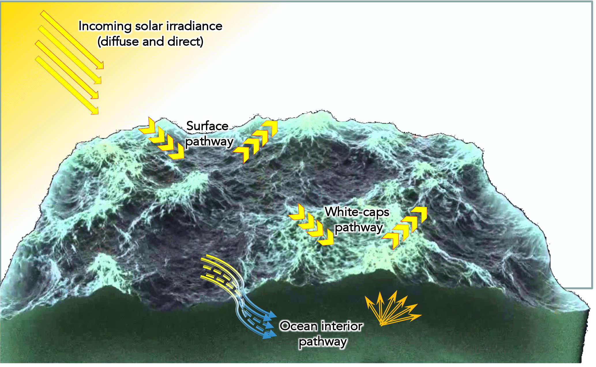
Figure 1Pathways of solar radiation over oceans as described in the new interactive scheme. Whitecaps, surface Fresnel, ocean interior influence of the reflection and the refraction of both direct and diffuse radiation.
The whitecaps originate from turbulence induced by the breaking of waves, which generates foam at the sea surface (Deane and Stokes, 2002; Melville and Matusov, 2002). In the absence of an ocean wave model such as WAM (e.g., Aouf et al., 2006; Ardhuin et al., 2010) which would provide more accurate whitecap coverage (WC) based on significant wave height (Bell et al., 2013; Woolf, 2005), we used the formulation of WC published in Salisbury et al. (2014). Their expression is based on recent spaceborne observations with a 37 GHz channel radar. It parametrizes WC as a function of the 10 m wind speed, w, in unit of m s−1:
As mentioned in Salisbury et al. (2014), this approximation of WC is valid for w ranging between 2 and 20 m s−1, which corresponds well to the range of w values simulated by the current generation of Earth system models. The formulation employed here does not account for the temperature dependence of wave breaking in agreement with other parameterizations for WC (Stramska, 2003) because its effect is weaker than that of surface winds on the whitecap coverage.
In order to solve the spectral dependence of the whitecap albedo, we use the relationship proposed by Whitlock et al. (1982). However, we rely on previous work indicating that the whitecap albedo of ordinary foam, αWC(λ), tends to be twice as small as that of fresh and dense foam (Koepke, 1984). We consequently apply a 1∕2 coefficient to the formulation proposed by Whitlock et al. (1982) for αWC(λ) from 400 to 2400 nm, as follows:
where rWC is the absorption coefficient of clear water in m−1. We use rWC(λ) as published in Whitlock et al. (1982) from 400 to 2400 nm. Outside the 400 to 2400 nm range, we chose to set rWC(λ) to zero due to the lack of available data in the literature. Tabulated values of αWC(λ) computed using this assumption are provided in Table S1 in the Supplement.
In the present scheme, we assume that whitecaps reflect equally direct and diffuse incoming solar radiation. We also assume that our formulation, which is based on observations, is not affected by the small contribution from the subsurface reflectance.
2.2 Treatment of the uncapped surface
2.2.1 Fresnel surface albedo for direct radiation
We describe the contribution of Fresnel reflection at the ocean surface, which is a major component of the OSA. Fresnel reflection is assumed to depend at a given wavelength (λ) on the solar zenith angle (θ), the refractive index of seawater (n) and the two-dimensional distribution of the ocean surface slopes (f). As mentioned earlier we neglect the dependence on the azimuthal angle of the incident radiation.
We follow Jin et al. (2011) and express the direct surface albedo ( as follows:
where μ=cos (θ), n is the spectral refractive index of seawater, rf is the Fresnel reflectance for a flat surface and f is a function that accounts for the distribution of multiple reflective facets at the ocean surface. Tabulated values for n(λ) are shown in Table S1. n0=1.34 corresponds to the refractive index of seawater averaged from 300 to 700 nm (i.e., visible spectrum) for which the f function is estimated.
The interaction of incident shortwave radiation with the multiple reflective facets of the ocean surface at various angles and directions is difficult to model. It is nonetheless possible to represent statistically the distribution of the slope of reflective ocean facets with a probabilistic function. The probabilistic function provided by Cox and Munk (1954) assumes a Gaussian distribution of mean slope facet as follows:
where ϑ is the facet angle, i.e., the angle between the normal to the facet and the normal to the horizontal ocean surface, and σ is the width the distribution of the facet angle. The parameter σ, also called the surface roughness, is modulated by the influence of surface (i.e., 10 m) wind speed (w) as . The formulation by Cox and Munk (1954) assume that (1) shading influence of ocean facets is neglected and (2) ocean surfaces never behave as a theoretical Fresnel surface (requiring σ=0). These approximations can impact calculation at high SZA and/or in absence of wind. In any case, this formulation (based on wind speed only) ignores the effect of the wind direction on the wind sea and the effect of swell, which both affect the distribution of slopes. This latter set of assumptions can also be revised in the foreseeable future when climate models include an interactive ocean wave model.
In order to account for various impacts of multiple ocean surface facets on including both multiple scattering (increasing surface reflection) and shading effect (reducing reflection), Jin et al. (2011) proposed expressing f as a polynomial function. This function intends to parameterize the mean contribution of multiple reflective facets at the ocean surface to using only the parameters μ and σ. This polynomial function is expressed as follows:
Coefficients of f have been fitted using several accurate calculations of using a radiative transfer model (Jin et al., 2006, 2005).
2.2.2 Fresnel surface albedo for diffuse radiation
The amount and distribution of incident diffuse radiation strongly depend on the amount and characteristics of cloud and aerosols. It is therefore difficult to derive an analytical formulation for from a BRDF that would be applicable to all atmospheric conditions. We therefore choose to use the simple expression for the diffuse surface albedo ( under cloudy sky proposed in Jin et al. (2011):
with σ and n defined as previously.
2.3 Contribution of the ocean interior reflectance to surface albedo
In this section, we describe the contribution of the ocean interior reflectance to the ocean surface albedo, αW. It is caused by solar radiation penetrating the ocean but eventually returning to the atmosphere after one or multiple reflections within the seawater volume. Below the ocean surface, solar radiation interacts not only with seawater but also with material in suspension in the water like the marine biological pigment or detrital organic materials (DOM). Previous studies show that DOM can influence radiative properties of the open ocean (e.g., Behrenfeld and Falkowski, 1997; Dutkiewicz et al., 2015; Kim et al., 2015). However, we chose to solely account for the influence of the marine biological pigment which is characterized by its chlorophyll content because the influence of DOM on ocean surface albedo is expected to be small compared to the surface chlorophyll. Furthermore the abundance of chlorophyll in seawater has been monitored from space for decades (e.g., Behrenfeld et al., 2001; Siegel et al., 2002; Yoder et al., 1993) by ocean color measurements. Such observations can provide a climatology to use in the climate model in absence of an ocean biogeochemical module.
Over the uncapped ocean surface, the fraction of direct radiation penetrating into the upper-most layer of the ocean interacts with the seawater, which has reflectance, R0. Upwelling radiation can be reflected downward at the air–sea interface with reflectance, rw. Therefore, the contribution of multiple reflections of penetrating radiation to the ocean albedo takes the form of the following Taylor series:
which can be arranged as follows:
We employ the formulation of rw and R0 proposed by Morel and Gentili (1991).
These authors express rw as a function of surface roughness σ, that is,
R0 represents an apparent optical property of seawater, which can be written as follows:
where aw(λ) and bw(λ) are the absorption and backscattering coefficients of seawater (in m−1); abp(λChl) and bbp(λChl) are absorption and backscattering coefficients of biological pigments (i.e., chlorophyll).
β(η,μ) is function of seawater and biological pigment backscattering and can be written as
where μ=cos (θ) and .
Backscattering of biological pigment, bbp, is computed using the formulation proposed in Morel and Maritorena (2001) which uses chlorophyll concentration, [Chl], as a surrogate of biological pigment concentration as follows:
with λ expressed here in nm and [Chl] in mg m−3. This formulation is valid for [Chl] ranging between 0.02 and 2 mg m−3.
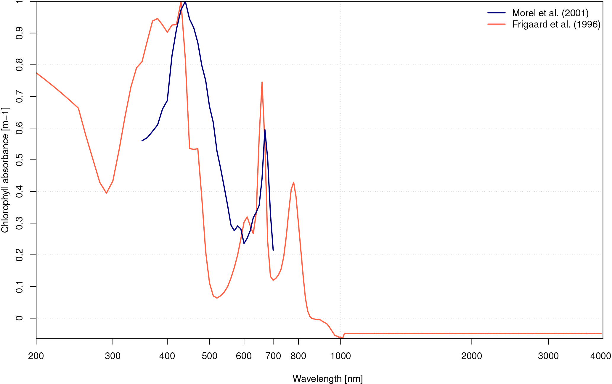
Figure 2Comparison of chlorophyll absorbance (m−1) as a function of wavelength (nanometers, in log scale) from Morel and Maritorena (2001) in blue and that of Frigaard et al. (1996) in red, which is used in the new interactive OSA scheme.
The absorption of biological pigment, abp(λChl), is also computed using Morel and Maritorena (2001) formalism:
where achl(λ) is the absorption of chlorophyll in m−1 and λ and [Chl] as previously defined.
Previous estimates of achl(λ), aw(λ) and bw(λ) used by Morel and Maritorena (2001) cover values for wavelengths ranging between 300 and 700 nm. Therefore, we have combined and interpolated several sets of tables of coefficients in order to solve consistently αW, and across the same range of wavelengths (i.e., from 200 to 4000 nm). aw(λ) has been derived from tables provided by Smith (1982) and Irvine and Pollack (1968), which span 200 to 800 and 800 to 4000 nm, respectively. achl(λ) has been derived from values published in Frigaard et al. (1996) which differ from those in Morel and Maritorena (2001; Fig. 2). bw(λ) is estimated from seawater backscattering coefficients published in Morel and Maritorena (2001) that have been interpolated from 300–700 to 200–4000 nm with polynomial splines. Tabulated values for achl(λ), aw(λ) and bw(λ) are given in Table S1.
The difference in the contribution of the ocean interior reflectance to the ocean surface albedo for direct and diffuse radiation essentially stems from the incident direction of incoming radiation. In the case of ocean interior reflectance for direct incoming radiation, , μ = cos (θ) whereas in the case of ocean interior reflectance for diffuse, , μ = 0.676. This value is considered an effective angle of incoming radiation of 47.47∘ according to Morel and Gentili (1991). Hence .
2.4 Computation of OSA
With the various components of OSA being now parameterized, the OSA for direct and diffuse radiation is estimated as follows:
Since detailed atmospheric radiative transfer (e.g., Clough et al., 2005; Mlawer et al., 1997) are now part of the current generation of Earth system models, most radiative codes resolve radiation from near-ultraviolet (∼ 200 nm) to near-infrared (∼ 4000 nm) wavelengths. Here, we design our scheme to compute both the spectral and broadband OSA. To this effect, the scheme computes the OSA from λ1=200 to λ2=4000 nm with a resolution of 10 nm. The contribution of each wavelength interval dλ to OSA is weighted by its amount of solar energy under the standard solar spectra ASTM E-490 AM0 (Shanmugam and Ahn, 2007), E(λ) assumption as follows.
Tabulated values for E(λ) are given in Table S1.
Finally for the total incoming radiation, the OSA can be written as follows:
where Fdir and Fdif are the downward surface fluxes of direct and diffuse radiation, respectively. OSA is then computed for each model ocean grid cell at each model time step. it should be noted that the SZA used in LMDZ is the average of the SZA during the daytime fraction of the time step.
In this section, we analyze the geographical structure of OSA which is decomposed as follows:
where Adir and Adif are the broadband ocean surface albedos for direct and diffuse radiation in the absence of whitecap albedo; AWC is the broadband albedo of whitecaps.
Adir, Adif and AWC have been estimated from offline calculations using ERA-Interim forcing fields from 2000 to 2009 at monthly frequency (Dee et al., 2011) and chlorophyll climatology from SeaWiFS (Siegel et al., 2002). Compared to Adir and Adif, AWC is constant in space; therefore its geographical structure arises from whitecap coverage (WC).
Figure 3a shows that Adir displays a strong meridional gradient with high values over high-latitude oceans and low values over the tropical oceans. It confirms that the solar zenith angle is the prominent driver of Adir. This albedo exhibits nonetheless geographical structures over the tropical oceans which are linked to the easterly wind regimes, suggesting that surface wind variability may have a small but noticeable influence on the ocean surface albedo for direct radiation.
Compared to Adir, Adif does not exhibit such a large meridional gradient (Fig. 3b). Adif shows values close to 0.06. It displays nonetheless values > 0.06 over the subtropical gyres and values < 0.06 over the North Atlantic and the Southern Ocean in response to the 10 m wind speeds. Those patterns are related to surface wind patterns but also to the geographical structure of oligotrophic gyres with low chlorophyll values which reinforce the contribution of the ocean interior reflectance to surface albedo for the diffuse incoming radiation.
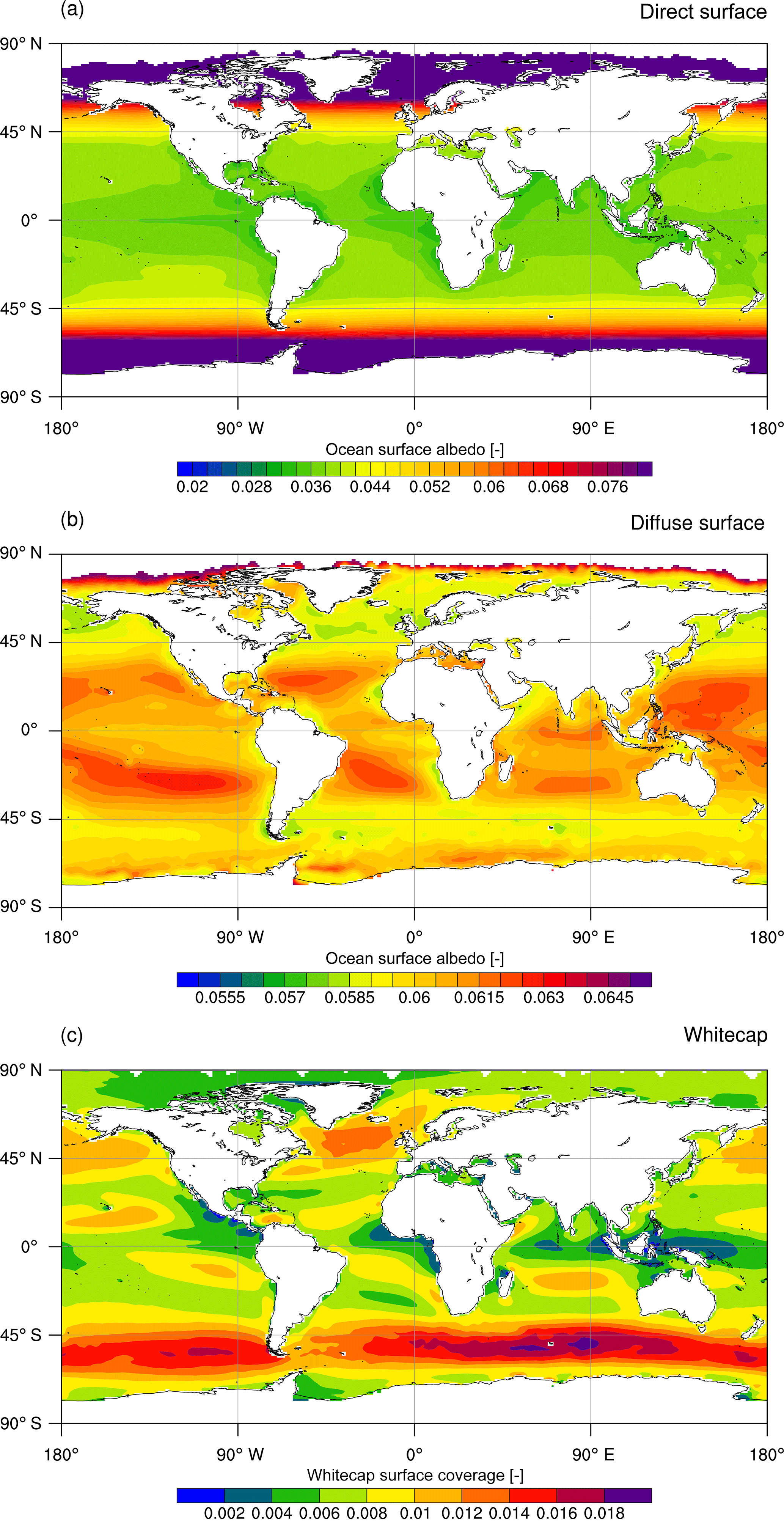
Figure 3Maps of ocean surface albedo for (a) direct and (b) diffuse radiation in the absence of whitecaps, and map of whitecaps surface coverage (c). Estimates are derived from offline calculation using ERA-Interim forcing fields (Dee et al., 2011) from years 2000 to 2012 and SeaWiFS chlorophyll climatology (Siegel et al., 2002) over years 1998–2007. Whitecap albedo is constant in space and is equal to 0.174.
Figure 3c provides further insight into the regional influence of WC which display a broadband albedo of 0.174. Offline calculation of WC shows that whitecaps influence albedo for direct and diffuse radiation where westerly winds blow regularly, for example, in the Southern Ocean, the North Atlantic and the North Pacific. A weaker but noticeable influence is also found over the tropical oceans.
While AWC is larger than Adir and Adif, the convolution of broadband albedo of the whitecaps and their coverage results in the maximum contribution of 0.003 to the broadband albedos for direct and diffuse radiation. However, its strong albedo makes the whitecaps an important factor at interannual and climate timescales. Indeed, this component of OSA for direct and diffuse radiation responds to the interannual variability of 10 m wind speed and also to climate change. Indeed, the contraction of Southern Ocean westerly winds (e.g., Böning et al., 2008) might induce subtle regional fluctuations in OSA that can feedback on the climate response.
4.1 Observations
To assess model reliability to simulate realistic OSA, we compare fields to available observations. For those observations, we estimate the time-averaged OSA from the ratio between the time-averaged upwelling and downwelling shortwave radiative fluxes provided in those data sets.
At local scale, we use the CERES Ocean Validation Experiment (COVE; Rutledge et al., 2006) ground-based measurements. This ocean platform instrument, located at Chesapeake Bay, has provided continuous measurements of several radiative fluxes since 2001. In this study, we use measurements of upwelling and downwelling global (i.e., direct and diffuse) shortwave radiation averaged across several instruments (https://cove.larc.nasa.gov/instruments.html).
At global scale, we perform model evaluation with retrievals from the CERES satellite radiation measurements (Wielicki et al., 1996). CERES data provides estimates of global shortwave radiation at top of the atmosphere and at the surface. In the present study, we focus on surface estimates since our analyses aims at assessing the representation of ocean surface albedo.
4.2 Models
4.2.1 LMDZ v5A
LMDZ is an atmospheric general circulation model developed at the Laboratoire de Météorologie Dynamique. The version of this atmosphere model, known as LMDZ v5A, is described in detail in Hourdin et al. (2013); it is part of the main IPSL climate model used for CMIP5 and described in Dufresne et al. (2013; IPSL-CM5A). The atmospheric resolution is 96 × 95 horizontally and 39 layers vertically. The old OSA scheme in this version of LMDZ is based on the formulation of Larsen and Barkstrom (1977). It is parameterized in terms of μ as follows:
Consequently, OSA varies between 0.0446 for a sun at zenith and 0.193 for a sun at the horizon. Direct and diffuse radiation are not distinguished, and only a broadband albedo is used in the visible spectrum (.
In LMDZ, the partitioning between direct and diffuse light is derived from the presence of clouds in the atmosphere model grid cell.
We assess simulated OSA using an atmosphere-only simulation with prescribed radiative forcing (greenhouse gases, aerosols, land-cover change) and fixed sea surface temperature as recommended by CMIP5 (Taylor et al., 2012). LMDZ has been integrated from 1979 up to 2012 under this protocol.
Similarly to the observations, simulated OSA at a given frequency is derived from the ratio between the time-averaged upwelling and downwelling shortwave radiative fluxes at that frequency.
4.2.2 ARPEGE-Climat v6.1
ARPEGE-Climat v6.1 derives from ARPEGE-Integrated Forecasting System (IFS), the operational numerical weather forecast models of Météo-France and the European Centre for Medium-range Weather Forecasts (ECMWF). Compared to the version used in Voldoire et al. (2013), several improvements in atmospheric physics have been implemented. They consist of a new vertical diffusion scheme which solves a prognostic turbulent kinetic energy equation following Cuxart et al. (2000), an updated prognostic microphysics representing the specific masses of cloud liquid and ice water, rain and snow, as detailed in Lopez (2002), and a new convection scheme known as the Prognostic Condensates Microphysics Transport (PCMT; Guérémy, 2011; Piriou et al., 2007). ARPEGE-Climat v6.1 is implicitly coupled to the surface model called SURFEX (Masson et al., 2013), which considers a diversity of surface formulations for the evolution of four types of surface: land, town, inland water and ocean. The old OSA formulation implemented in SURFEX follows Taylor et al. (1996). This scheme enables the computation of as a function of μ:
Since this schema does not enable computation of , it is set to a constant value of 0.066.
Like LMDZ, the partitioning of direct and diffuse radiation depends on the cloud cover in the atmospheric model grid cell.
Simulations performed with ARPEGE-Climat also consists of AMIP simulations as in LMDZ, except for sea surface temperature which relies on data recommended by CMIP6 (Eyring et al., 2016a). This simulation also spans 1979 to 2012.
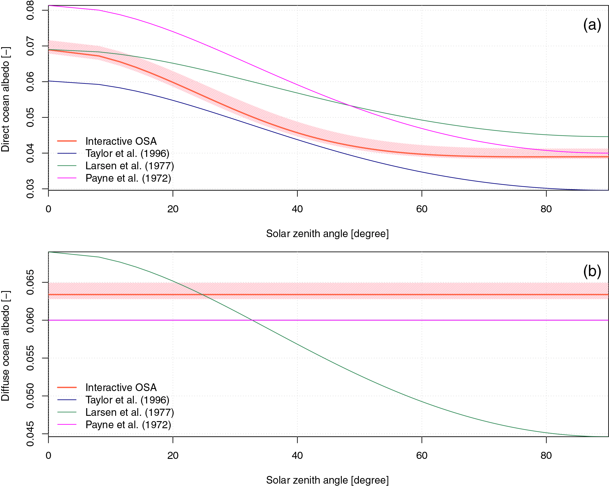
Figure 4Analytical solution for (a) direct and (b) diffuse ocean surface albedo as used in Taylor et al. (1996) and Larsen and Barkstrom (1977), and computed solution for the new interactive ocean surface albedo scheme, as a function of solar zenith angle. Analytical solution for direct and diffuse ocean surface albedo as derived from Payne (1972) formulation is also represented in both panels, because this parameterization is currently used in a number of state-of-the-art atmospheric and ocean models. Hatching depicts potential variations related to changes in 10 m wind speed and surface chlorophyll.
Analyses are complemented using another simulation of ARPEGE-Climat in which the resolved dynamics is nudged towards that of ERA-Interim. Nudging consists of restoring the model wind divergence and vorticity and the surface pressure towards those from ERA-Interim. The restoring timescale is 12 h for the wind divergence and surface pressure and 6 h for the wind vorticity. This simulation is employed hereafter as a kind of reference of what could be expected by the OSA parameterization if the wind spatiotemporal properties were “realistic”. In this case, only the direct-to-diffuse incident radiation partitioning remains tied to ARPEGE-Climat. This simulation replicates the chronology of the observed day-to-day variability of 10 m wind speed and hence is expected to be closer to the ground-based observations.
For those models simulations, simulated OSA at a given frequency is determined from the ratio between the time-averaged upwelling and downwelling shortwave radiative fluxes at that frequency.
In order to better understand changes in simulated OSA, we compare first the analytical solution of old and new interactive OSA schemes used in the two atmospheric models for both direct and diffuse radiation (Fig. 4). We also compare old and new interactive OSA schemes to Payne (1972) OSA scheme that is currently used in a number of atmospheric and ocean models such as NEMO (Madec, 2008).
Figure 4a shows that old OSA schemes for direct radiation differ in terms of response to solar zenith angle. Indeed, for a given solar zenith angle, the scheme used in LMDZ (Larsen and Barkstrom, 1977) leads to a greater OSA than that used in ARPEGE-Climat (Taylor et al., 1996). The shape of the response to variations in solar zenith angle suggests that the scheme used in ARPEGE-Climat leads to a slightly stronger meridional gradient in OSA than that used in LMDZ. Interestingly, the new scheme produces OSA values bracketed by those of old algorithms, except for small solar zenith angle. Under this condition, the effect of winds is to increase OSA up to 0.072. It also displays a greater response to variations in solar zenith angle which differs substantially from those given by the old schemes.
Compared to the Payne (1972) OSA scheme, old and new schemes used in the two atmosphere models exhibit a weaker meridional gradient in OSA (Fig. 4a). However, the meridional gradient as estimated by Payne (1972) is similar to that produced by Taylor et al. (1996) because their formulations solely differ by a coefficient; that is, 0.037 for Taylor et al. (1996) and 0.05 for Payne (1972).
Differences in OSA for diffuse radiation presented in Fig. 4b are noticeable. They clearly illustrate modeling assumptions in the old schemes. Indeed, old schemes have been built on ad hoc formulations. Neither Taylor et al. (1996) nor Larsen and Barkstrom (1977) have provided a differentiated OSA for direct and diffuse radiation. This is why OSA for diffuse radiation is set to 0.06 (corresponding to the angular average of the OSA for direct radiation) in ARPEGE-Climat, whereas that of LMDZ is equal to the OSA for direct radiation from Larsen and Barkstrom (1977).
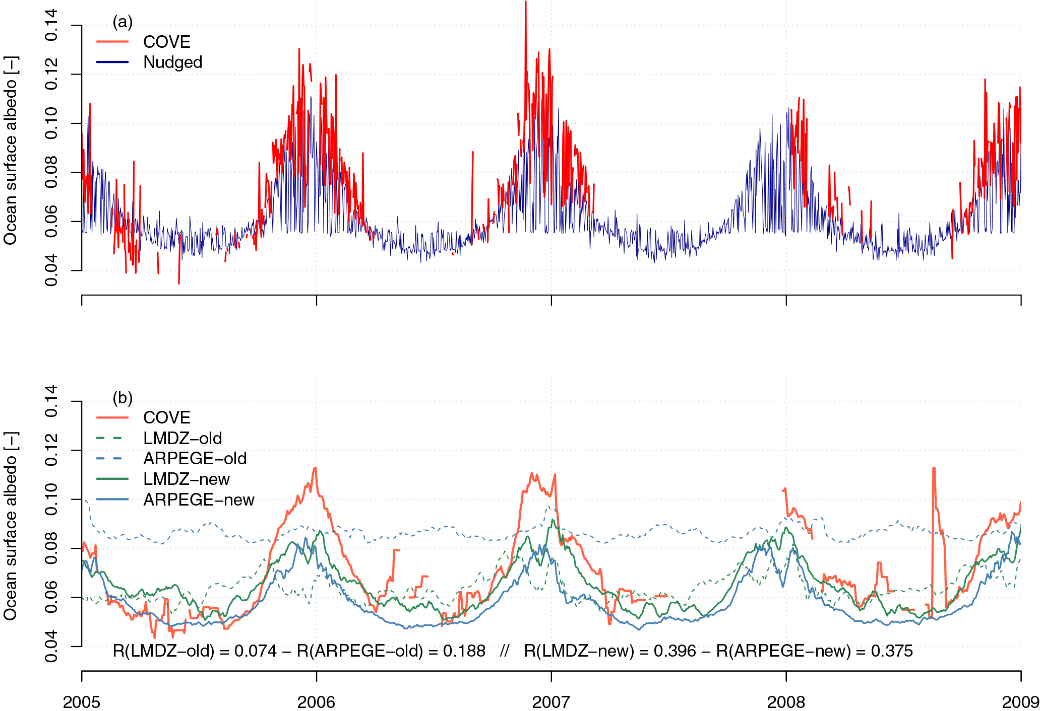
Figure 5Ocean surface albedo at COVE station (36.905∘ N, 75.713∘ W) from 2005 to 2009. Panel (a) compares daily mean time series of ocean surface albedo as derived from ground-based observations (in red) and as reconstructed with ARPEGE-Climat nudged toward ERA-Interim (dark blue). Panel (b) displays, for the sake of clarity, time series of daily mean ocean surface albedo smoothed using a 5-day moving average for both observations and model results. All daily mean time series from 2001 to 2015 are displayed in Fig. S1. Ocean surface albedo simulated by ARPEGE-Climat (in blue) and LMDZ (in green) using the old and new interactive scheme are indicated with dashed and solid lines, respectively.
Figure 4b shows that the new interactive scheme displays features similar to the diffuse OSA used in ARPEGE-Climat or that estimated from Payne (1972). This scheme produces nonetheless slightly larger values which can fluctuate in response to other drivers. The old OSA for diffuse radiation employed in LMDZ responds to variations in solar zenith angle although it should not. Errors related to this erroneous representation of OSA for diffuse radiation are also modulated by the partitioning between direct and diffuse radiation estimated by the atmospheric model.

Figure 6Probability density function of daily mean ocean surface albedo at COVE station (36.905∘ N, 75.713∘ W) derived from daily mean time series over years 2001 to 2013. Ocean surface albedo derived from ground-based observations and as reconstructed with ARPEGE-Climat nudged toward ERA-Interim are indicated in red and dark blue, respectively. Ocean surface albedo simulated by ARPEGE-Climat (in blue) and LMDZ (in green) using the old and new interactive scheme are indicated with dashed and solid lines, respectively.
In this section, we employ COVE daily data to assess the simulated OSA by both atmospheric models at local scale. OSA is computed here as the ratio of up-to-down radiation fluxes averaged at daily resolution for both ground-based observations and models. Such an evaluation is fundamental because it relies on direct ground-truth observations over the ocean surface and hence provides a more accurate assessment of the OSA scheme as compared to the global-scale satellite-derived estimates developed in the following sections.
Figure 5 shows how well the model using old and new interactive OSA scheme behaves at daily frequency compared to the ground-based observations at COVE station from 2001 to 2009. Figures 5 and S1a clearly show that both old OSA schemes of ARPEGE-Climat and LMDZ fail at replicating day-to-day OSA variations at the COVE station. Comparatively, Figs. 5 and S1b emphasize how much the new interactive scheme improves OSA as simulated by both atmospheric models. Indeed, the simulated OSA values are now consistent with observation at COVE station, with temporal correlation greater than 0.3. However, the models fail at replicating the large OSA values occurring during the winter in ground-based observations.
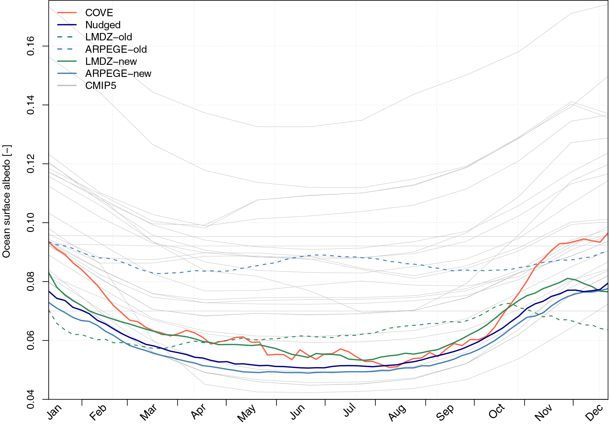
Figure 7Mean seasonal cycle of ocean surface albedo at COVE station (36.905∘ N, 75.713∘ W) derived from daily mean time series over years 2001 to 2013. Ocean surface albedo derived from ground-based observations and as reconstructed with ARPEGE-Climat nudged toward ERA-Interim are indicated in red and dark blue, respectively. Ocean surface albedo simulated by ARPEGE-Climat (in blue) and LMDZ (in green) using the old and new interactive scheme are indicated with dashed and solid lines, respectively. For comparison, the mean seasonal cycle of ocean surface albedo at COVE as simulated by available CMIP5 models is represented by thin grey lines.
Those findings are reinforced when we compare the probability density function (pdf) estimated from daily mean OSA as simulated by models against that derived from ground-based observations (Fig. 6). This analysis provides further insight into how old and new interactive OSA schemes behave at COVE station. Figure 6 confirms that old schemes fail at capturing the day-to-day variations in OSA. Indeed, day-to-day variations in OSA estimated from old schemes arise from day-to-day variations in SZA and to a lesser extent to variations in direct-to-diffuse ratio of incident radiation which is related to the cloud cover. As shown in Fig. 4, old OSA schemes crudely represent diffuse albedo. Therefore, errors in direct-to-diffuse ratio of incident radiation incurs errors in the simulated OSA. Consequently, day-to-day variations are better reproduced when the albedo for diffuse radiation is realistically simulated (Fig. 6). In particular, the new interactive scheme captures the minimum OSA values occurring during the summer which are lower than 0.06.
At seasonal scale, OSA estimated from averaged radiative fluxes agrees with the above-mentioned findings for ground-based observations and models. Figure 7 clearly shows that old OSA schemes do not capture seasonal variations of observed OSA. Correlation between observation-derived OSA and that simulated by both models is 0.32 for ARPEGE-Climat and 0.28 for LMDZ, which is very low, indicating an unrealistic representation of OSA. Comparison with CMIP5 atmosphere models shows that OSA as simulated by ARPEGE-Climat or LMDZ is in the range of CMIP5 models (0.04–0.17), confirming the large uncertainties related to simulated OSA in a state-of-the-art climate model. While several CMIP5 models replicate seasonal variation in OSA, most of them exhibit large biases in simulated OSA compared to the observation-based estimate. Only ACCESS1-3, BNU-ESM, HadCM3, MIROC-ESM and MIROC-ESM-CHEM display a mean seasonal cycle of OSA comparable to the observation-based estimate at COVE station. For ARPEGE-Climat, this erroneous representation of OSA at seasonal-scale leads, at least for this location, to a systematic bias in the surface energy budget of +3 W m−2 in winter and −1.5 W m−2 in summer. It is thus likely that large deviation in OSA as simulated by CMIP5 leads to substantial errors in energy flow at the air–sea interface.
Figure 7 shows significant improvements in the simulated OSA in both models using the new interactive scheme. In both models, the simulated seasonal cycle of OSA replicates the minimum observed during the summer, although with the new interactive OSA scheme, both models do not capture large values of OSA of 0.10 occurring during the winter. That said, model–data comparison shows that correlation with observations has been improved. Indeed, correlation between observed and simulated daily values over a mean yearly cycle has increased from 0.23 to 0.84 in LMDZ to 0.32 to 0.86 in ARPEGE-Climat.
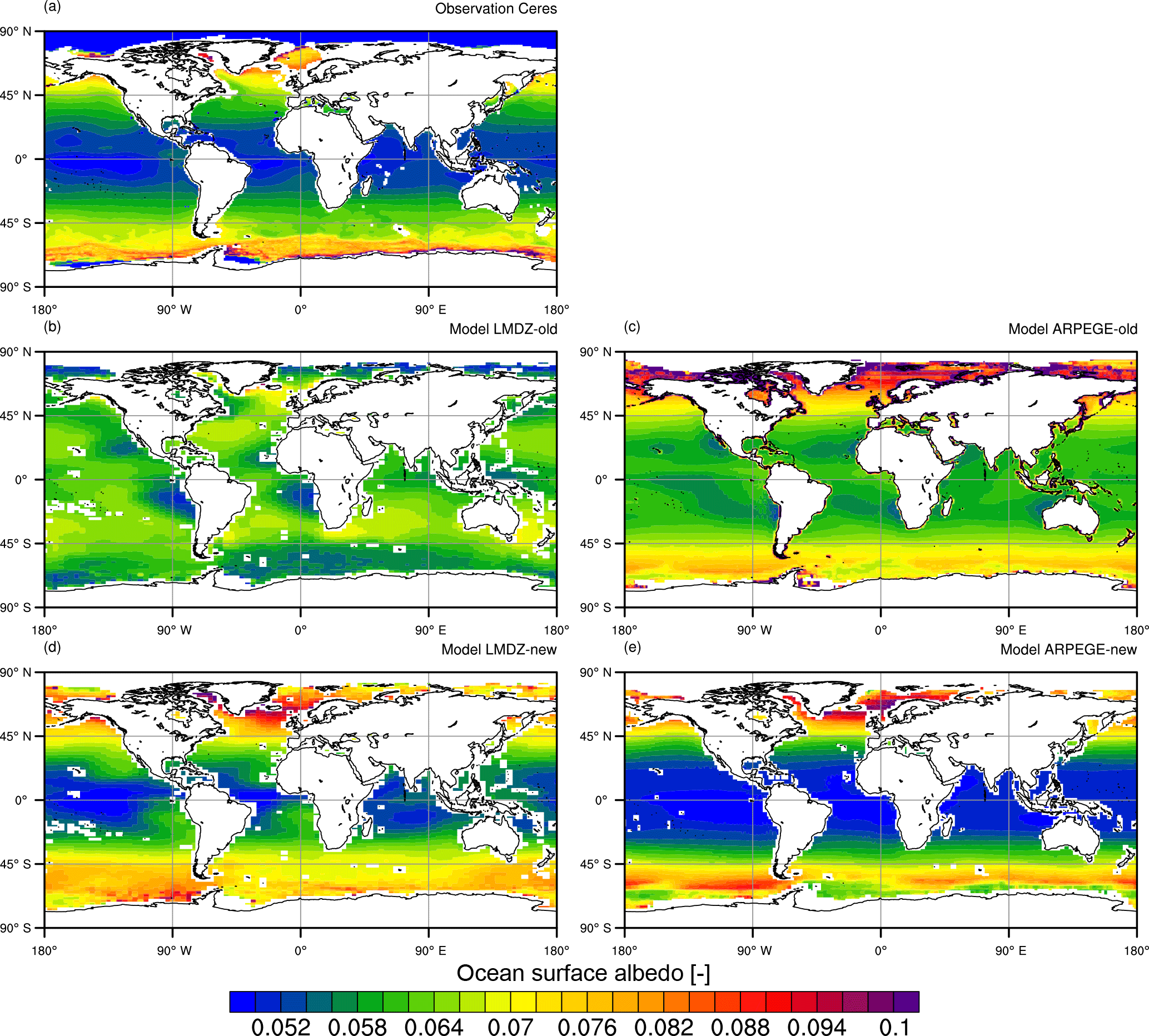
Figure 8Decadal-mean climatology ocean surface albedo as (a) estimated from CERES satellite observations (Wielicki et al., 1996) and as simulated by LMDZ (b, d) and ARPEGE-Climat (c, e). In panels (b) and (c), LMDZ and ARPEGE-Climat use old ocean albedo schemes, that is, Taylor et al. (1996) and Larsen and Barkstrom (1977), respectively. In panels (d) and (e), LMDZ and ARPEGE-Climat use employ the new interactive ocean surface albedo scheme. Decadal-mean climatology is derived from radiative fluxes averaged over years 2001 to 2014 for CERES estimates and 2000 to 2012 for both climates models.
Although improved, Figs. 5, 6 and 7 show that new interactive OSA scheme seems to suffer from a systematic bias in winter and miss OSA values greater than 0.10. This is supported by the fact that this systematic bias is displayed for all model estimates independently from the atmospheric physics and dynamics (i.e., LMDZ, ARPEGE-Climat and nudged OSA). That being said, some other possible reasons can explain such deviations between models and ground-based data. First, current atmosphere models suffer from systematic errors in the ratio of direct-to-diffuse radiation which could be related to bias in cloud cover or aerosol optical thickness (as shown in Fig. S2). A greater-than-observed atmospheric optical depth in winter may favor the diffuse path over the direct path, resulting in a lower-than-observed OSA. Second, coarse-resolution atmospheric models are not able to replicate the mesoscale meteorological and oceanic conditions at this very location. Differences in surface wind between the models and field conditions can increase the contribution of whitecap albedo with the respect to that of the Fresnel reflectance. Third, local ocean conditions and the presence of ocean waves resulting from remote wind (i.e., swells) are not simulated by the atmospheric models. This would lead to an underestimation of the contributions of both whitecaps and Fresnel reflectance.
7.1 Climatological mean
This section details the evaluation of OSA at the global scale using global satellite product that are routinely used in Earth system model evaluation (Eyring et al., 2016b; Gleckler et al., 2008). We thus use OSA retrieved from CERES surface product to assess the simulated OSA by ARPEGE-Climat and LMDZ.
Figure 8 presents geographical pattern of OSA as simulated by ARPEGE-Climat and LMDZ using Taylor et al. (1996) and Larsen and Barkstrom (1977) schemes, respectively. These old OSA schemes were used during CMIP5 and thus give an idea of the errors in the models' radiative budgets.
Globally, the simulated OSA overestimates the CERES-derived estimate (∼ 0.058) by about 0.007. However, the most striking feature is the substantial differences in the meridional structure. CERES-derived OSA shows maximum values over the high-latitude oceans and minimum values over the tropical oceans. None of the models using old schemes are able to capture this meridional structure. Deviations are particularly high for LMDZ, which only barely replicate maximum OSA over high-latitude oceans and minimum OSA over tropical oceans. Both models exhibit poor spatial correlation with −0.03 for LMDZ and 0.40 for ARPEGE-Climat. Model–data errors in OSA mirror model bias in surface upwelling shortwave radiation, which amounts to ∼ 7 W m−2 over the tropical oceans compared to CERES.
The new interactive scheme improves favorably the comparison with observations (Fig. 8). Indeed global mean OSA is equal to 0.062 for LMDZ and 0.057 for ARPEGE-Climat, which better matches the value derived from CERES data. As such, the model bias in surface upwelling shortwave radiation has been reduced by ∼ 1 W m−2 on average over the ocean and by up to ∼ 5 W m−2 over the tropical oceans.
Both models capture the meridional structure of the OSA with spatial correlations of about 0.82 for LMDZ and 0.86 for ARPEGE-Climat. Nonetheless, the simulated OSA displays some biases. In LMDZ and ARPEGE-Climat, the modeled OSA over the North Atlantic is slightly overestimated and shifted to the south. Major differences between simulated OSA are noticeable over the tropical oceans, where models differ in terms of zonal structure. LMDZ displays OSA of ∼ 0.06 over eastern boundary upwelling systems, which is slightly too high compared to CERES. Differences in the OSA geographical structure between ARPEGE-Climat and LMDZ arise from differences in 10 m wind speed (Fig. S3) and direct-to-diffuse incident radiation as determined from the simulated cloud cover (Fig. S4). Large-scale deviations between models and observations seem to be related to differences in 10 m wind fields (Fig. S3). Model–data deviations in OSA at the regional scale rather mirror biases in total cloud cover (Fig. S4). This is especially clear over low-latitude oceans where LMDZ overestimates OSA over the eastern boundary upwelling systems where LMDZ overestimates the cloud cover (Fig. S4). This result is expected since over the low-latitude oceans the contribution of diffuse OSA is stronger than that of direct OSA (Figs. 3 and 4).
7.2 Seasonal variability
Figure 9 compares the simulated and CERES-derived OSA on the seasonal scale. This timescale matters for accurately modeling the Earth's climate because the flow of incoming radiation fluctuates up to 1 order of magnitude between winter and summer at high latitudes.
Figure 9a, b and c show that both models using old OSA schemes only just reproduce the seasonal cycle of OSA derived from CERES. This is particularly the case for LMDZ, which produced an unrealistic seasonal cycle for OSA. LMDZ fails at simulating maximum OSA during the winter of both hemispheres. Instead, extreme values of simulated OSA occur at 50∘ N and 50∘ S during the summer. Simulated OSA in ARPEGE-Climat does not present these features but is biased high during all seasons.
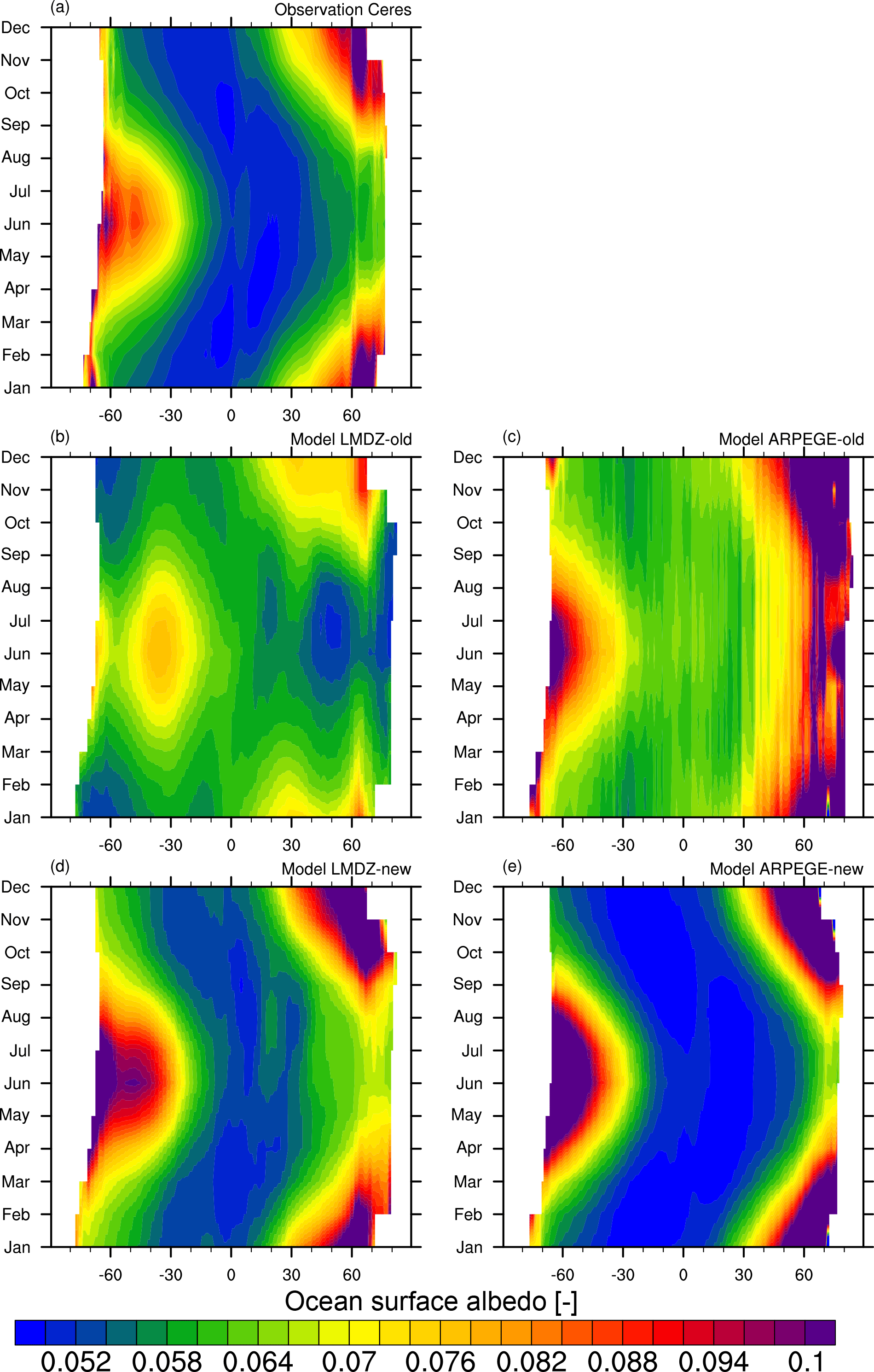
Figure 9Hovmöller diagram representing the zonally averaged ocean surface albedo as a function of month. The various panels display the ocean surface albedo as (a) estimated from CERES satellite observations (Wielicki et al., 1996) and as simulated by (b) LMDZ and (c) ARPEGE-Climat using old ocean albedo schemes, that is, Taylor et al. (1996) and Larsen and Barkstrom (1977), respectively. Panels (d) and (e) show OSA as simulated by the new interactive ocean surface albedo scheme for LMDZ and ARPEGE-Climat, respectively. Monthly means are derived from radiative fluxes averaged over years 2001 to 2014 for CERES estimates and from years 2000 to 2012 for both climates models.
With the new interactive scheme, the seasonal OSA is improved in both models (Fig. 9d, e). The simulated OSA matches that derived from CERES at seasonal scale, with high values during the winter and low values between 30∘ S and 30∘ N. Improvement is especially noticeable for LMDZ which captures the observed seasonal cycle of OSA.
However, a few errors remain in the simulated OSA. In LMDZ, OSA is slightly too high compared to CERES (∼ 0.002) in boreal and austral summer. Nonetheless, simulated OSA reproduces realistic OSA values in the tropics (∼ 0.052). In ARPEGE-Climat, instead, the simulated OSA seems slightly too low compared to CERES (∼ −0.002). This leads ARPEGE-Climat to overestimate the fraction of low-OSA ocean. Interestingly this bias solely concerns the tropical oceans. Indeed, simulated OSA over high-latitude oceans displays realistic features at the seasonal scale. The fact that errors in ARPEGE-Climat and LMDZ are of different signs tends to suggest that the new interactive scheme is not intrinsically biased. It rather points to biases in driving fields such as the surface wind speeds or the ratio between direct and diffuse shortwave radiation simulated by either ARPEGE-Climat or LMDZ (Fig. S2).
In this paper, we have detailed a new interactive scheme for ocean surface albedo suited for Earth system models. This scheme computes the ocean surface albedo accounting for the spectral dependence (across a range of wavelengths between 200 and 4000 nm), the characteristics of incident solar radiation (direct of diffuse), the effects of surface winds, chlorophyll content and whitecaps and the canonical solar zenith angle dependence. This scheme enables improved air–sea exchange of solar radiation. It thus provides a much more physical basis to resolve the radiative transfer at the interface between the atmosphere and the upper ocean and offer a suite of processes that are included in complex stand-alone ocean radiative transfer software such as HYDROLIGHT (Ohlman et al., 2000). This work can be extended to include coupling to an ocean wave model that would provide a more realistic distribution of ocean surface state.
Although direct and diffuse albedos were included in the old ocean albedo schemes of the two atmospheric models used here, our results demonstrate that their assumptions employed for diffuse albedo (i.e., fixed values or equal to the direct albedo) are not realistic. The new interactive scheme improves its representation which leads to substantially reduced model–data error in ocean surface albedo over the low-latitude oceans.
Comparison to available data set shows, for at least two state-of-the-art climate models, a noticeable improvement in terms of simulated ocean surface albedo compared to their old ocean surface albedo schemes. At the global scale, the geographical pattern of simulated ocean surface albedo has been improved in both models. The simulated seasonal cycle also shows a noticeable improvement, especially in LMDZ, with a better correlation to CERES data (up to 0.8). At the local scale, simulated ocean surface albedo also fits ocean surface albedo derived from ground-based radiative measurements at daily resolution with an improved correlation up to 0.8.
Compared to old schemes, the new interactive scheme is more complex and induces a small increase in elapsed model time of about 0.2 %. Although noticeable, this increase does not preclude centennial-long simulation or high-resolution model simulations.
Improved ocean surface albedo might lead to differences in the simulated climate or marine biogeochemistry dynamics which will be assessed in future work. Indeed, a difference of about 1 % of simulated ocean surface albedo for a global mean irradiance of ∼ 180 W m−2 can induce a deviation in the energy flow of the Earth system comparable to the impact of land-cover changes over land (Myhre et al., 2013).
The interactive ocean surface albedo code detailed in the paper is a part of the SURFEX (V8.0) ocean scheme and is available as open-source material via http://www.cnrm-game-meteo.fr/surfex/. SURFEX (V8.0) is updated at a relatively low frequency (every 3 to 6 months) and the developments presented in this paper are available starting from SURFEX (V8.0). If more frequent updates are needed, or if what is required is not in Open-SURFEX (DrHOOK, FA/LFI formats, GAUSSIAN grid), you are invited to set up an SVN account to access real-time modifications of the code (see the instructions at the previous link). In any case, all the tabulated values use for this algorithm are available in the Supplement.
The supplement related to this article is available online at: https://doi.org/10.5194/gmd-11-321-2018-supplement.
The authors declare that they have no conflict of interest.
This work was supported by the H2020 project CRESCENDO (Coordinated Research
in Earth Systems and Climate: Experiments, kNowledge, Dissemination and
Outreach), which received funding from the European Union's Horizon 2020
research and innovation programme under grant agreement no. 641816; the Labex
L-IPSL, which is funded by the ANR (grant no. ANR-10-LABX-0018); and by the
European FP7 IS-ENES2 project (grant no. 312979). The LMDZ simulations in
this work were performed using TGCC resources as part of the GENCI (Grand
Equipement National de Calcul Intensif) computer time allocation (grant 2016-t2014012201).
Edited by: Robert Marsh
Reviewed by: two anonymous referees
Allen, M. R., Frame, D. J., Huntingford, C., Jones, C. D., Lowe, J. A., Meinshausen, M., and Meinshausen, N.: Warming caused by cumulative carbon emissions towards the trillionth tonne, Nature, 458, 1163–1166, https://doi.org/10.1038/nature08019, 2009.
Aouf, L., Lefevre, J.-M., and Hauser, D.: Assimilation of Directional Wave Spectra in the Wave Model WAM: An Impact Study from Synthetic Observations in Preparation for the SWIMSAT Satellite Mission, J. Atmos. Ocean. Tech., 23, 448–463, https://doi.org/10.1175/JTECH1861.1, 2006.
Ardhuin, F., Rogers, E., Babanin, A. V., Filipot, J.-F., Magne, R., Roland, A., van der Westhuysen, A., Queffeulou, P., Lefevre, J.-M., Aouf, L., and Collard, F.: Semiempirical Dissipation Source Functions for Ocean Waves. Part I: Definition, Calibration, and Validation, J. Phys. Oceanogr., 40, 1917–1941, https://doi.org/10.1175/2010JPO4324.1, 2010.
Behrenfeld, M. J. and Falkowski, P. G.: Photosynthetic rates derived from satellite-based chlorophyll concentration, Limnol. Oceanogr., 42, 1–20, https://doi.org/10.4319/lo.1997.42.1.0001, 1997.
Behrenfeld, M. J., Randerson, J. T., McClain, C. R., Feldman, G. C., Los, S. O., Tucker, C. J., Falkowski, P. G., Field, C. B., Frouin, R., Esaias, W. E., Kolber, D. D., and Pollack, N. H.: Biospheric Primary Production During an ENSO Transition, Science, 291, 2594–2597, https://doi.org/10.1126/science.1055071, 2001.
Bell, T. G., De Bruyn, W., Miller, S. D., Ward, B., Christensen, K. H., and Saltzman, E. S.: Air–sea dimethylsulfide (DMS) gas transfer in the North Atlantic: evidence for limited interfacial gas exchange at high wind speed, Atmos. Chem. Phys., 13, 11073–11087, https://doi.org/10.5194/acp-13-11073-2013, 2013.
Böning, C. W., Dispert, A., Visbeck, M., Rintoul, S. R., and Schwarzkopf, F. U.: The response of the Antarctic Circumpolar Current to recent climate change, Nat. Geosci., 1, 864–869, https://doi.org/10.1038/ngeo362, 2008.
Chandrasekhar, S.: Radiative heat transfer, Dover Publications, New York, USA, 11, 11–12, 1960.
Clough, S. A., Shephard, M. W., Mlawer, E. J., Delamere, J. S., Iacono, M. J., Cady-Pereira, K., Boukabara, S., and Brown, P. D.: Atmospheric radiative transfer modeling: a summary of the AER codes, J. Quant. Spectrosc. Ra., 91, 233–244, 2005.
Cox, C. and Munk, W.: Measurement of the Roughness of the Sea Surface from Photographs of the Sun's Glitter, J. Opt. Soc. Am., 44, 838–850, 1954.
Cuxart, J., Bougeault, P., and Redelsperger, J. L.: A turbulence scheme allowing for mesoscale and large-eddy simulations, Q. J. Roy. Meteor. Soc., 126, 1–30, https://doi.org/10.1002/qj.49712656202, 2000.
Deane, G. B. and Stokes, M. D.: Scale dependence of bubble creation mechanisms in breaking waves, Nature, 418, 839–844, https://doi.org/10.1038/nature00967, 2002.
Dee, D. P., Uppala, S. M., Simmons, A. J., Berrisford, P., Poli, P., Kobayashi, S., Andrae, U., Balmaseda, M. A., Balsamo, G., Bauer, P., Bechtold, P., Beljaars, A. C. M., van de Berg, L., Bidlot, J., Bormann, N., Delsol, C., Dragani, R., Fuentes, M., Geer, A. J., Haimberger, L., Healy, S. B., Hersbach, H., Hólm, E. V., Isaksen, L., Kållberg, P., Köhler, M., Matricardi, M., McNally, A. P., Monge-Sanz, B. M., Morcrette, J. J., Park, B. K., Peubey, C., de Rosnay, P., Tavolato, C., Thépaut, J. N., and Vitart, F.: The ERA-Interim reanalysis: configuration and performance of the data assimilation system, Q. J. Roy. Meteor. Soc., 137, 553–597, 2011.
Dufresne, J.-L., Foujols, M. A., Denvil, S., Caubel, A., Marti, O., Aumont, O., Balkanski, Y., Bekki, S., Bellenger, H., Benshila, R., Bony, S., Bopp, L., Braconnot, P., Brockmann, P., Cadule, P., Cheruy, F., Codron, F., Cozic, A., Cugnet, D., Noblet, N., Duvel, J. P., Ethe, C., Fairhead, L., Fichefet, T., Flavoni, S., Friedlingstein, P., Grandpeix, J. Y., Guez, L., Guilyardi, E., Hauglustaine, D., Hourdin, F., Idelkadi, A., Ghattas, J., Joussaume, S., Kageyama, M., Krinner, G., Labetoulle, S., Lahellec, A., Lefebvre, M.-P., Lefèvre, F., Lévy, C., Li, Z. X., Lloyd, J., Lott, F., Madec, G., Mancip, M., Marchand, M., Masson, S., Meurdesoif, Y., Mignot, J., Musat, I., Parouty, S., Polcher, J., Rio, C., Schulz, M., Swingedouw, D., Szopa, S., Talandier, C., Terray, P., Viovy, N., and Vuichard, N.: Climate change projections using the IPSL-CM5 Earth System Model: from CMIP3 to CMIP5, Clim. Dynam., 40, 2123–2165, https://doi.org/10.1007/s00382-012-1636-1, 2013.
Dutkiewicz, S., Hickman, A. E., Jahn, O., Gregg, W. W., Mouw, C. B., and Follows, M. J.: Capturing optically important constituents and properties in a marine biogeochemical and ecosystem model, Biogeosciences, 12, 4447–4481, https://doi.org/10.5194/bg-12-4447-2015, 2015.
Eyring, V., Bony, S., Meehl, G. A., Senior, C. A., Stevens, B., Stouffer, R. J., and Taylor, K. E.: Overview of the Coupled Model Intercomparison Project Phase 6 (CMIP6) experimental design and organization, Geosci. Model Dev., 9, 1937–1958, https://doi.org/10.5194/gmd-9-1937-2016, 2016a.
Eyring, V., Gleckler, P. J., Heinze, C., Stouffer, R. J., Taylor, K. E., Balaji, V., Guilyardi, E., Joussaume, S., Kindermann, S., Lawrence, B. N., Meehl, G. A., Righi, M., and Williams, D. N.: Towards improved and more routine Earth system model evaluation in CMIP, Earth Syst. Dynam., 7, 813–830, https://doi.org/10.5194/esd-7-813-2016, 2016b.
Frigaard, N.-U., Larsen, K. L., and Cox, R. P. A.: Spectrochromatography of photosynthetic pigments as a fingerprinting technique for microbial phototrophs, FEMS Microbiol. Ecol., 20, 69–77, https://doi.org/10.1111/j.1574-6941.1996.tb00306.x, 1996.
Frölicher, T. L.: Climate response: Strong warming at high emissions, Nat. Clim. Change, 6, 823–824, https://doi.org/10.1038/nclimate3053, 2016.
Frouin, R., Schwindling, M., and Deschamps, P.-Y.: Spectral reflectance of sea foam in the visible and near-infrared: In situ measurements and remote sensing implications, J. Geophys. Res., 101, 14361–14371, https://doi.org/10.1029/96JC00629, 1996.
Frouin, R., Iacobellis, S. F., and Deschamps, P. Y.: Influence of oceanic whitecaps on the Global Radiation Budget, Geophys. Res. Lett., 28, 1523–1526, https://doi.org/10.1029/2000GL012657, 2001.
Gillett, N. P., Arora, V. K., Matthews, D., and Allen, M. R.: Constraining the Ratio of Global Warming to Cumulative CO2 Emissions Using CMIP5 Simulations, J. Climate, 26, 6844–6858, https://doi.org/10.1175/JCLI-D-12-00476.s1, 2013.
Gleckler, P. J., Taylor, K. E., and Doutriaux, C.: Performance metrics for climate models, J. Geophys. Res., 113, D06104, https://doi.org/10.1029/2007JD008972, 2008.
Gordon, H. R. and Wang, M.: Influence of oceanic whitecaps on atmospheric correction of ocean-color sensors, Appl. Optics, 33, 7754–7763, https://doi.org/10.1364/AO.33.007754, 1994.
Guérémy, J. F.: A continuous buoyancy based convection scheme: one- and three-dimensional validation, Tellus A, 63, 687–706, https://doi.org/10.1111/j.1600-0870.2011.00521.x, 2011.
Gupta, S., Ritchey, N., Wilber, A., and Whitlock, C.: A climatology of surface radiation budget derived from satellite data, J. Climate, 12, 2691–2710, https://doi.org/10.1175/1520-0442(1999)012<2691:ACOSRB>2.0.CO;2, 1999.
Hansen, J., Russell, G., Rind, D., Stone, P., Lacis, A., Lebedeff, S., Ruedy, R., and Travis, L.: Efficient Three-Dimensional Global Models for Climate Studies: Models I and II, Mon. Weather Rev., 111, 609–662, https://doi.org/10.1175/1520-0493(1983)111<0609:ETDGMF>2.0.CO;2, 1983.
Hense, I., Stemmler, I., and Sonntag, S.: Ideas and perspectives: climate-relevant marine biologically driven mechanisms in Earth system models, Biogeosciences, 14, 403–413, https://doi.org/10.5194/bg-14-403-2017, 2017.
Hourdin, F., Foujols, M.-A., Codron, F., Guemas, V., Dufresne, J.-L., Bony, S., Denvil, S., Guez, L., Lott, F., Ghattas, J., Braconnot, P., Marti, O., Meurdesoif, Y., and Bopp, L.: Impact of the LMDZ atmospheric grid configuration on the climate and sensitivity of the IPSL-CM5A coupled model, Clim. Dynam., 40, 2167–2192, https://doi.org/10.1007/s00382-012-1411-3, 2013.
IPCC: Climate Change 2001: The Scientific Basis, edited by: Houghton, T. J., Ding, Y., Griggs, D. J., Noguer, M., van der Linden, P. J., Dai, X., Maskell, K., and Johnson, C. A., Cambridge University Press, Cambridge, UK and New York, NY, USA, 2001.
IPCC: Climate Change 2007: The Physical Science Basis, edited by: Solomon, S., Qin, D., Manning, M., Chen, Z., Marquis, M., Averyt, K. B., Tignor, M., and Miller, H. L., Cambridge University Press, Cambridge, UK and New York, NY, USA, 2007.
IPCC: Climate Change 2013: The Physical Science Basis, edited by: Stoker, T. F., Qin, D., Plattner, G., Tignor, M., Allen, S. K., Boschung, J., Nauels, A., Xia, Y., Bex, V., and Midgley, P. M., Cambridge Univ Press, Cambridge, UK and New York, NY, USA, 2013.
Irvine, W. M. and Pollack, J. B.: Infrared optical properties of water and ice spheres, Icarus, 8, 324–360, 1968.
Jin, Z., Charlock, T. P., and Rutledge, K.: Analysis of Broadband Solar Radiation and Albedo over the Ocean Surface at COVE, J. Atmos. Ocean. Tech., 19, 1585–1601, https://doi.org/10.1175/1520-0426(2002)019<1585:AOBSRA>2.0.CO;2, 2002.
Jin, Z., Charlock, T. P., Smith Jr., W. L., and Rutledge, K.: A parameterization of ocean surface albedo, Geophys. Res. Lett., 31, L22301, https://doi.org/10.1029/2004GL021180, 2004.
Jin, Z., Charlock, T. P., Rutledge, K., Cota, G., Kahn, R., Redemann, J., Zhang, T., Rutan, D. A., and Rose, F.: Radiative transfer modeling for the CLAMS experiment, J. Atmos. Sci., 62, 1053–1071, 2005.
Jin, Z., Charlock, T. P., Rutledge, K., Stamnes, K., and Wang, Y.: Analytical solution of radiative transfer in the coupled atmosphere-ocean system with a rough surface, Appl. Optics, 45, 7443–7455, 2006.
Jin, Z., Qiao, Y., Wang, Y., Fang, Y., and Yi, W.: A new parameterization of spectral and broadband ocean surface albedo, Opt. Express, 19, 26429–26443, 2011.
Kent, E. C., Forrester, T. N., and Taylor, P. K.: A comparison of oceanic skin effect parameterizations using shipborne radiometer data, J. Geophys. Res., 101, 16649, https://doi.org/10.1029/96JC01054, 1996.
Kim, G. E., Pradal, M.-A., and Gnanadesikan, A.: Quantifying the biological impact of surface ocean light attenuation by colored detrital matter in an ESM using a new optical parameterization, Biogeosciences, 12, 5119–5132, https://doi.org/10.5194/bg-12-5119-2015, 2015.
Koepke, P.: Effective reflectance of oceanic whitecaps, Appl. Optics, 23, 1816–1824, https://doi.org/10.1364/AO.23.001816, 1984.
Larsen, J. C. and Barkstrom, B. R.: Effects of realistic angular reflection laws for the Earth's surface upon calculations of the Earth-atmosphere albedo, Radiation in the Atmosphere, Proceedings of an International Symposium, Princeton, USA, Science Press, p. 451, 1977.
Li, J., Scinocca, J., Lazare, M., McFarlane, N., von Salzen, K., and Solheim, L.: Ocean Surface Albedo and Its Impact on Radiation Balance in Climate Models, J. Climate, 19, 6314–6333, https://doi.org/10.1175/JCLI3973.1, 2006.
Li, T., Bai, Y., Li, G., He, X., Chen, C.-T., Gao, K., and Liu, D.: Effects of ultraviolet radiation on marine primary production with reference to satellite remote sensing, Front. Earth Sci., 9, 237–247, https://doi.org/10.1007/s11707-014-0477-0, 2015.
Lopez, P.: Implementation and validation of a new prognostic large-scale cloud and precipitation scheme for climate and data-assimilation purposes, Q. J. Roy. Meteor. Soc., 128, 229–257, https://doi.org/10.1256/00359000260498879, 2002.
Madec, G.: NEMO ocean engine, Note du Pôle de modélisation, Vol. 27, Institut Pierre-Simon Laplace (IPSL), Paris, France, No. 27, 2008.
Masson, V., Le Moigne, P., Martin, E., Faroux, S., Alias, A., Alkama, R., Belamari, S., Barbu, A., Boone, A., Bouyssel, F., Brousseau, P., Brun, E., Calvet, J.-C., Carrer, D., Decharme, B., Delire, C., Donier, S., Essaouini, K., Gibelin, A.-L., Giordani, H., Habets, F., Jidane, M., Kerdraon, G., Kourzeneva, E., Lafaysse, M., Lafont, S., Lebeaupin Brossier, C., Lemonsu, A., Mahfouf, J.-F., Marguinaud, P., Mokhtari, M., Morin, S., Pigeon, G., Salgado, R., Seity, Y., Taillefer, F., Tanguy, G., Tulet, P., Vincendon, B., Vionnet, V., and Voldoire, A.: The SURFEXv7.2 land and ocean surface platform for coupled or offline simulation of earth surface variables and fluxes, Geosci. Model Dev., 6, 929–960, https://doi.org/10.5194/gmd-6-929-2013, 2013.
Melville, W. K. and Matusov, P.: Distribution of breaking waves at the ocean surface, Nature, 417, 58–63, https://doi.org/10.1038/417058a, 2002.
Mlawer, E. J., Taubman, S. J., Brown, P. D., Iacono, M. J., and Clough, S. A.: Radiative transfer for inhomogeneous atmospheres: RRTM, a validated correlated-k model for the longwave, J. Geophys. Res., 102, 16663–16682, https://doi.org/10.1029/97JD00237, 1997.
Morel, A. and Antoine, D.: Heating rate within the upper ocean in relation to its bio-optical state, J. Phys. Oceanogr., 24, 1652–1665, https://doi.org/10.1175/1520-0485(1994)024<1652:HRWTUO>2.0.CO;2, 1994.
Morel, A. and Gentili, B.: Diffuse reflectance of oceanic waters: its dependence on Sun angle as influenced by the molecular scattering contribution, Appl. Optics, 30, 4427–4438, https://doi.org/10.1364/AO.30.004427, 1991.
Morel, A. and Maritorena, S.: Bio-optical properties of oceanic waters: A reappraisal, J. Geophys. Res.-Oceans, 1106, 7163–7180, https://doi.org/10.1029/2000JC000319, 2001.
Murtugudde, R., Beauchamp, J., and McClain, C. R.: Effects of penetrative radiation on the upper tropical ocean circulation, J. Climate, 15, 470–486, https://doi.org/10.1175/1520-0442(2002)015<0470:EOPROT>2.0.CO;2, 2002.
Myhre, G., Shindell, D., Bréon, F.-M., Collins, W., Fuglestvedt, J., Huang, J., Koch, D., Lamarque, J.-F., Lee, D., Mendoza, B., Nakajima, T., Robock, A., Stephens, G., Takemura, T., and Zhang, H.: Anthropogenic and Natural Radiative Forcing, in: Climate Change 2013: The Physical Science Basis. Contribution of Working Group I to the Fifth Assessment Report of the Intergovernmental Panel on Climate Change, edited by: Stocker, T. F., Qin, D., Plattner, G.-K., Tignor, M., Allen, S. K., Doschung, J., Nauels, A., Xia, Y., Bex, V., and Midgley, P. M., Cambridge University Press, 659–740, https://doi.org/10.1017/CBO9781107415324.018, 2013.
Myhre, G., Boucher, O., Breon, F.-M., Forster, P., and Shindell, D.: Declining uncertainty in transient climate response as CO2 forcing dominates future climate change, Nat. Geosci., 8, 181–185, https://doi.org/10.1038/ngeo2371, 2015.
Nelson, D. M. and Smith, W. O. J.: The role of light and major nutrients, Limnol. Oceanogr., 36, 1650–1661, 1991.
Ohlmann, J. C. and Siegel, D. A.: Ocean Radiant Heating. Part II: Parameterizing Solar Radiation Transmission through the Upper Ocean, J. Phys. Oceanogr., 30, 1849–1865, https://doi.org/10.1175/1520-0485(2000)030<1849:ORHPIP>2.0.CO;2, 2000.
Ohlmann, J. C., Siegel, D. A., and Mobley, C. D.: Ocean Radiant Heating. Part I: Optical Influences, J. Phys. Oceanogr., 30, 1833–1848, https://doi.org/10.1175/1520-0485(2000)030<1833:ORHPIO>2.0.CO;2, 2000.
Otto, A., Otto, F. E. L., Boucher, O., Church, J., Hegerl, G., Forster, P. M., Gillett, N. P., Gregory, J., Johnson, G. C., Knutti, R., Lewis, N., Lohmann, U., Marotzke, J., Myhre, G., Shindell, D., Stevens, B., and Allen, M. R.: Energy budget constraints on climate response, 6, 415–416, https://doi.org/10.1038/ngeo1836, 2013.
Payne, R. E.: Albedo of the Sea Surface, J. Atmos. Sci., 29, 959–970, https://doi.org/10.1175/1520-0469(1972)029<0959:AOTSS>2.0.CO;2, 1972.
Piriou, J.-M., Redelsperger, J.-L., Geleyn, J.-F., Lafore, J.-P., and Guichard, F.: An Approach for Convective Parameterization with Memory: Separating Microphysics and Transport in Grid-Scale Equations, J. Atmos. Sci., 64, 4127–4139, https://doi.org/10.1175/2007JAS2144.1, 2007.
Preisendorfer, R. W. and Mobley, C. D.: Albedos and Glitter Patterns of a Wind-Roughened Sea Surface, J. Phys. Oceanogr., 16, 1293–1316, https://doi.org/10.1175/1520-0485(1986)016<1293:AAGPOA>2.0.CO;2, 1986.
Rutledge, C. K., Schuster, G. L., Charlock, T. P., Denn, F. M., Smith Jr., W. L., Fabbri, B. E., Madigan Jr., J. J., and Knapp, R. J.: Offshore Radiation Observations for Climate Research at the CERES Ocean Validation Experiment: A New “Laboratory” for Retrieval Algorithm Testing, B. Am. Meteorol. Soc., 87, 1211–1222, https://doi.org/10.1175/BAMS-87-9-1211, 2006.
Salisbury, D. J., Anguelova, M. D., and Brooks, I. M.: Global Distribution and Seasonal Dependence of Satellite-based Whitecap Fraction, Geophys. Res. Lett., 41, 1616–1623, https://doi.org/10.1002/2014GL059246, 2014.
Shanmugam, P. and Ahn, Y. H.: Reference solar irradiance spectra and consequences of their disparities in remote sensing of the ocean colour, Ann. Geophys., 25, 1235–1252, https://doi.org/10.5194/angeo-25-1235-2007, 2007.
Siegel, D. A., Doney, S. C., and Yoder, J. A.: The North Atlantic spring phytoplancton bloom and the Sverdrup's critical depth hypothesis, Science, 296, 730–733, https://doi.org/10.1126/science.1069174, 2002.
Smith, E. D.: Water Characteristics, J. Water Pollut. Con. F., 54, 541–554, 1982.
Smyth, T. J.: Penetration of UV irradiance into the global ocean, J. Geophys. Res., 116, C11020, https://doi.org/10.1029/2011JC007183, 2011.
Stramska, M.: Observations of oceanic whitecaps in the north polar waters of the Atlantic, J. Geophys. Res., 108, 3086, https://doi.org/10.1029/2002JC001321, 2003.
Taylor, J. P., Edwards, J. M., Glew, M. D., Hignett, P., and Slingo, A.: Studies with a flexible new radiation code. II: Comparisons with aircraft short-wave observations, Q. J. Roy. Meteor. Soc., 122, 839–861, https://doi.org/10.1002/qj.49712253204, 1996.
Taylor, K. E., Stouffer, R. J., and Meehl, G. A.: An Overview of CMIP5 and the Experiment Design, B. Am. Meteorol. Soc., 93, 485–498, https://doi.org/10.1175/BAMS-D-11-00094.1, 2012.
Voldoire, A., Sanchez-Gomez, E., Salas y Mélia, D., Decharme, B., Cassou, C., Sénési, S., Valcke, S., Beau, I., Alias, A., Chevallier, M., Déqué, M., Deshayes, J., Douville, H., Fernandez, E., Madec, G., Maisonnave, E., Moine, M. P., Planton, S., Saint-Martin, D., Szopa, S., Tyteca, S., Alkama, R., Belamari, S., Braun, A., Coquart, L., and Chauvin, F.: The CNRM-CM5.1 global climate model: description and basic evaluation, Clim. Dynam., 40, 2091–2121, https://doi.org/10.1007/s00382-011-1259-y, 2013.
Whitlock, C. H., Bartlett, D. S., and Gurganus, E. A.: Sea foam reflectance and influence on optimum wavelength for remote sensing of ocean aerosols, Geophys. Res. Lett., 9, 719–722, https://doi.org/10.1029/GL009i006p00719, 1982.
Wielicki, B. A., Barkstrom, B. R., Harrison, E. F., Lee III, R. B., Louis Smith, G., and Cooper, J. E.: Clouds and the Earth's Radiant Energy System (CERES): An Earth Observing System Experiment, B. Am. Meteorol. Soc., 77, 853–868, https://doi.org/10.1175/1520-0477(1996)077<0853:CATERE>2.0.CO;2, 1996.
Woolf, D. K.: Effect of wind waves on air–sea gas exchange: proposal of an overall CO2 transfer velocity formula as a function of breaking-wave parameter, Tellus B, 57, 478–487, https://doi.org/10.1023/A:1021215904955, 2005.
Yoder, J., McClain, C., Feldman, G., and Esaias, W.: Annual Cycles of Phytoplankton Chlorophyll Concentrations in the Global Ocean – a Satellite View, Global Biogeochem. Cy., 7, 181–193, https://doi.org/10.1029/93GB02358, 1993.
- Abstract
- Introduction
- Interactive ocean surface albedo parameterization
- Contribution of various OSA components
- Materials and methods
- Comparison of analytical calculation
- Evaluation at COVE station (36.905∘ N, 75.713∘ W)
- Global-scale evaluation
- Conclusions
- Code availability
- Competing interests
- Acknowledgements
- References
- Supplement