Direct relation graph (DRG) is a method for generating subsets of detailed chemical mechanisms by removing species that have a negligible effect on a predefined set of target species. In the original version of the DRG method developed by Lu and Law (2005), the DIC r_T,B between a target species T and a non-target species B is defined as

where ${\dot{w}}_{i,T}$ is the net rate of species T from reaction i, and δ_i,B is an index specifying the existence of B in reaction i. The net rate of a species from a general reversible reaction is calculated using ${\dot{w}}_{i,T}={\mathit{\nu }}_{i,T}\cdot {\dot{w}}_i^r$, where ν_i,T is the difference in the stoichiometric coefficients of species T in reaction i, and ${\dot{w}}_i^r$ is the net rate of reaction i. The index δ_i,B is equal to 1 if B exists in reaction i, and 0 otherwise. Clearly, $\mathrm{0}\le r_{T,B}\le \mathrm{1}$, and r_T,B is generally not equal to r_B,T. A large value of r_T,B implies that species B is important in the evaluation of the rate of T, while a low value implies that it is not as important. A threshold (ϵ) is introduced, and provided $r_{T,B}>\mathit{ϵ}$, species B is added to the set of dependent species of T, otherwise it is deemed unimportant and removed. This relation is denoted as a direct path T→B. An example of a DRG involving four species A, B, C, and D, is given in Fig. 1 with the numbers indicating the values of the DICs for each pair. The process is repeated for all target species T_i, and the final set of species in the skeletal mechanism is constructed from the union of all target species sets. Species not included in the union set are eliminated, as are reactions involving any of the eliminated species.

Figure 1Example of a direct relation graph involving four species.

Download

DRG has been applied with good overall results in a number of studies in combustion research, yet the simple definition of the interaction coefficient in Eq. (1) has some important limitations. Consider the model situation depicted in Fig. 1. If A is the target species and C is the species in question, then with an example threshold value (ϵ) of 0.1, C would be added to the dependent set of A. However, it is clear that “stronger”, i.e., more important paths from A to C exist, for example, A → B → C. Thus, the notion of “path” becomes important, and a suitable DIC definition is required able to describe this. In addition, there are also alternative paths, e.g., A → D → C or A → D → B → C.

The DRGEP method aims to account for the above points by using an improved DIC definition and reduction strategy. In DRGEP (Niemeyer and Sung, 2011; Pepiot-Desjardins and Pitsch, 2008), the DIC is first defined using

where the production P_T and consumption terms C_T of T are defined as

and

The DIC, as defined above, is calculated for all species. The path interaction coefficient (PIC) $r_{T,B}^p$ for a given path p connecting target species T and B is then defined as

i.e., it is the product of all DICs along that path. The PIC is calculated for all possible paths connecting T to B, and an overall path interaction coefficient (OIC), $r_{T,B}^{\text{o}}$ is then calculated using

i.e., the strongest path from T to B is identified based on the product of the DICs of connected nodes across all paths linking T and B. In the example in Fig. 1, the strongest path is A → B → C. This is due to the fact that for this path $r_{\text{A–C}}^{\text{o}}=\mathrm{0.9}\cdot \mathrm{0.7}=\mathrm{0.63}$, which is the largest value, and both B and C are included in the set of A. The process is repeated for all target species of interest, and species with overall interaction coefficients less than a predefined threshold value are removed.

The identification of the strongest path is a common problem in computational science, and a number of different route-finding algorithms have been developed for this task. In this study, we employ a classic algorithm for searching through the connected nodes and obtaining $r_{T,B}^{\text{o}}$, which equates to the “strongest” path (Dijkstra, 1959). An in-house code, namely REDCHEM_ v0.0 was specifically developed for the DRGEP method, and for all associated functions including the route-finding subroutines.

Reduction methods require input data, and these data should be representative of the actual reaction scenario. This translates to using actual weather-forecast simulation data as input for the DRGEP method. However, this is hardly ever done in practice, as there is a large computational overload for conducting these kinds of simulations in the first place. As a result, a computationally more efficient initial-value problem (box model) is used as a model scenario for the reduction, which is common practice in chemical mechanism reduction studies (Dunker, 1986; Heard et al., 1998; Neophytou et al., 2004). The species mixing ratios C_i evolve according to

where G_i are non-linear functions of the species rates, with initial conditions $C_i^{\mathrm{0}}$ for the species mixing ratios, and T⁰ for temperature. The pressure is kept fixed at 1.0 atm, and the temperature at 298.0 K. The kinetic pre-processor library (KPP) (Daescu et al., 2003; Damian et al., 2002; Sandu et al., 2003) is used for the numerical integration of Eq. (7). The KPP library includes a number of different solvers, and in this study a 5-stage Runge–Kutta method (Hairer and Wanner, 1993; Hairer et al., 1993) was used from the package (Radau5). This method is stiffly accurate and robust, and is often used for benchmarking purposes.

Table 1Initial species mixing ratios (ppbv) for RACM as deduced from Heard et al. (1998). Water content is 10⁷ ppbv, CO content is 2310 ppbv. Pressure is fixed at 1 atm, and temperature at 298 K. VOC∕NO_x ratios (methane not included) for cases A–F are 4.2, 10.7, 19.1, 4.4, 11.1, and 19.8.

Download Print Version | Download XLSX

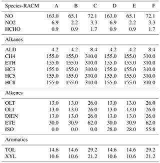
Six different initial scenarios are considered. The species mixing ratios for each model scenario are given in Table 1. These model scenarios were used by Heard et al. (1998) for reducing the CBMEX mechanism using sensitivity analysis. In this work, the same mixing ratios are used as per Table 1 of Heard et al. (1998), but are adapted for the chemical mechanism used in this study. In this paper we group important alkane, alkene, and aromatic species for each mechanism, and initialize their mixing ratios based on the relevant alkane, alkene, and aromatic species found in the study of Heard et al. (1998). Cases A–C correspond to increasing VOC∕NO_x ratios not including isoprene, while cases D–F correspond to about the same VOC∕NO_x ratios with isoprene included. The VOC∕NO_x ratios are relatively high, and this ensures that a large number of VOC-relevant reactions are activated; thus, in this process a relatively large region of the composition space is covered. At the same time we are interested in ozone production in relatively highly polluted areas where such conditions are typically found.

The J values for the photolysis rate coefficients are based on parameterizations as developed in the MCM (Derwent et al., 1998). These are given by

where θ is the solar azimuth angle, and I, M, and N are reaction-specific constants. A 48 h run is conducted for each scenario, which results in a total of 496 datasets. These scenarios are used as input for DRGEP and the reduction process is done on a dataset basis. Important species are retained for each dataset, and the process is repeated for the next dataset. Any new species not already included in the dataset is added. Once all datasets are considered, a species union set is formed, and any reactions involving species other than those included in the species union set are removed. The target species is set to be O₃, which is an important pollutant of interest. In addition, O₃ is eventually produced by the degradation of the VOCs through a large number of reaction pathways; therefore, it is a good target for the reduction.

Table 2Overall interaction coefficients (OICs) for target O₃ (top 35) for case A at t=12 and t=24 h.

Download Print Version | Download XLSX

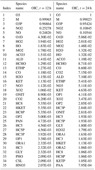
As an example, Table 2 lists the OIC values for target O₃ as obtained for scenario A at midday (t=12 h) and midnight (t=24 h). Clearly, there is a difference in the OIC values for each species since the rate constants depend on the solar azimuth angle which determines the rate constants of the photolytic reactions. Top scoring species for O₃ include third-body species M, and oxygen species such as O3P (ground-state oxygen atom) and O1D (excited state oxygen atom). This is expected since these species readily react to produce O₃ through the reactions $\mathrm{O}\mathrm{3}\mathrm{P}+\mathrm{M}\Rightarrow {\mathrm{O}}_{\mathrm{3}}$ and $\mathrm{O}\mathrm{1}\mathrm{D}+\mathrm{M}\Rightarrow {\mathrm{O}}_{\mathrm{3}}$. Nitrogen oxides NO and NO₂ also score high as they too react both directly and indirectly with ozone. Direct paths include the reactions ${\mathrm{O}}_{\mathrm{3}}+\mathrm{NO}\Rightarrow {\mathrm{NO}}_{\mathrm{2}}+{\mathrm{O}}_{\mathrm{2}}$ and ${\mathrm{O}}_{\mathrm{3}}+{\mathrm{NO}}_{\mathrm{2}}\Rightarrow {\mathrm{NO}}_{\mathrm{3}}+{\mathrm{O}}_{\mathrm{2}}$, while indirect paths include reactions with O3P. The methyl peroxy radical MO₂ ranks high as it is involved in numerous reactions with VOCs. The hydroxyl radical HO also scores high since it is the main oxidation path of the VOCs which eventually end up producing ozone. With a threshold of $\mathrm{9.0}\times {\mathrm{10}}^{-\mathrm{3}}$ (which results in a 54-species subset as explained later in the text), 18 species will be included in the set for t=12 h, and 11 species will be included for t=24 h. The process is then repeated for all other datasets to form the overall species union set for the target O₃.

In order to quantify the quality of the skeletal mechanisms generated using DRGEP, a percentage error is defined based on the target species of interest, i.e., ozone. For a mixing ratio obtained using the skeletal mechanism $C_i^{\text{s}}$, and a mixing ratio using the detailed mechanism $C_i^{\text{d}}$, this is defined as

where N is the total number of cases. Note that zero values are not taken into account for the error calculation.

Figure 2Ozone mixing ratio percentage error against the number of species in the skeletal RACM mechanism.

Download

Figure 2 shows this error against the number of species in the skeletal mechanism. As expected, the error increases as more species are removed. With about 10 species removed (75 to 65) the error is negligibly small. The error then increases once more than about 10 species are removed; however, the error remains small down to about 55 species (20 species removed) at less than 10 %. The huge spike in the error below about 55 species results from the removal of important intermediates.

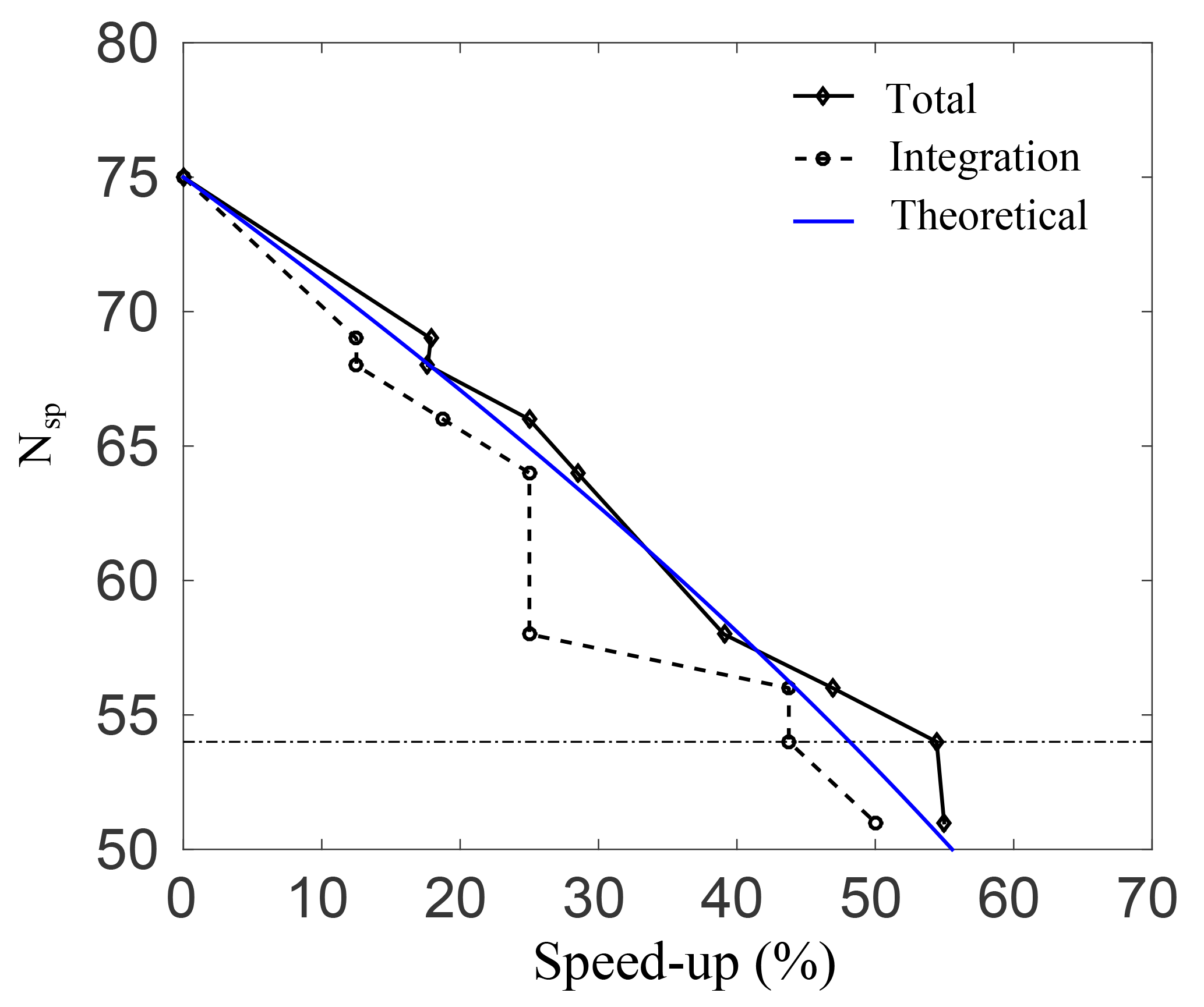
Figure 3Number of species plotted against the percentage speed-up for the total simulation time, and for integrating Eq. (7) alone.

Download

Figure 3 shows the percentage speed-up (CPU time) gained, against the number of species in the skeletal mechanisms. This is done for case A, and similar results were observed for the rest of the cases. The speed-up is calculated for both the total simulation time, and for integrating Eq. (3) alone. The threshold line where the error in O₃ prediction spikes as per the results in Fig. 2 is also shown. Clearly, as the number of species is reduced, the computational time drops and there is an increase in both speed-ups. It is interesting to note that for a decrease from 64 to 58 species there is no increase in integration speed-up. This implies that the stiffness of the remaining species and equations is unchanged. Nevertheless, there is an increase in the total speed-up of almost 10 % for a decrease from 64 to 58 species, which is due to simulation overheads alone and is quite significant. The average speed-up due to overhead computations is found to be 6.6 %. At the threshold error (e) of 10 %, the smallest possible skeletal mechanism contains 54 species and 150 reactions (the threshold for OIC at this point is $\mathrm{9.0}\times {\mathrm{10}}^{-\mathrm{3}}$), which is significantly smaller than the detailed mechanism.

For this mechanism, the total speed-ups and integration speed-ups are 54.4 % and 43.7 %, respectively. In general, the CPU time scales with the total number of species in the system due to the evaluation of the Jacobian when dealing with stiff systems. For integration of the system alone, the expected speed-up percentage scales as speed-up $\left(\mathit{\%}\right)=\mathrm{100}\cdot \left|\right(N_{\text{sp}}/N_{\text{sp,det}}{)}^{\mathrm{2}}-\mathrm{1}|$, and this is shown as a blue line in Fig. 3. Clearly, there is a good qualitative agreement with the theoretical result.

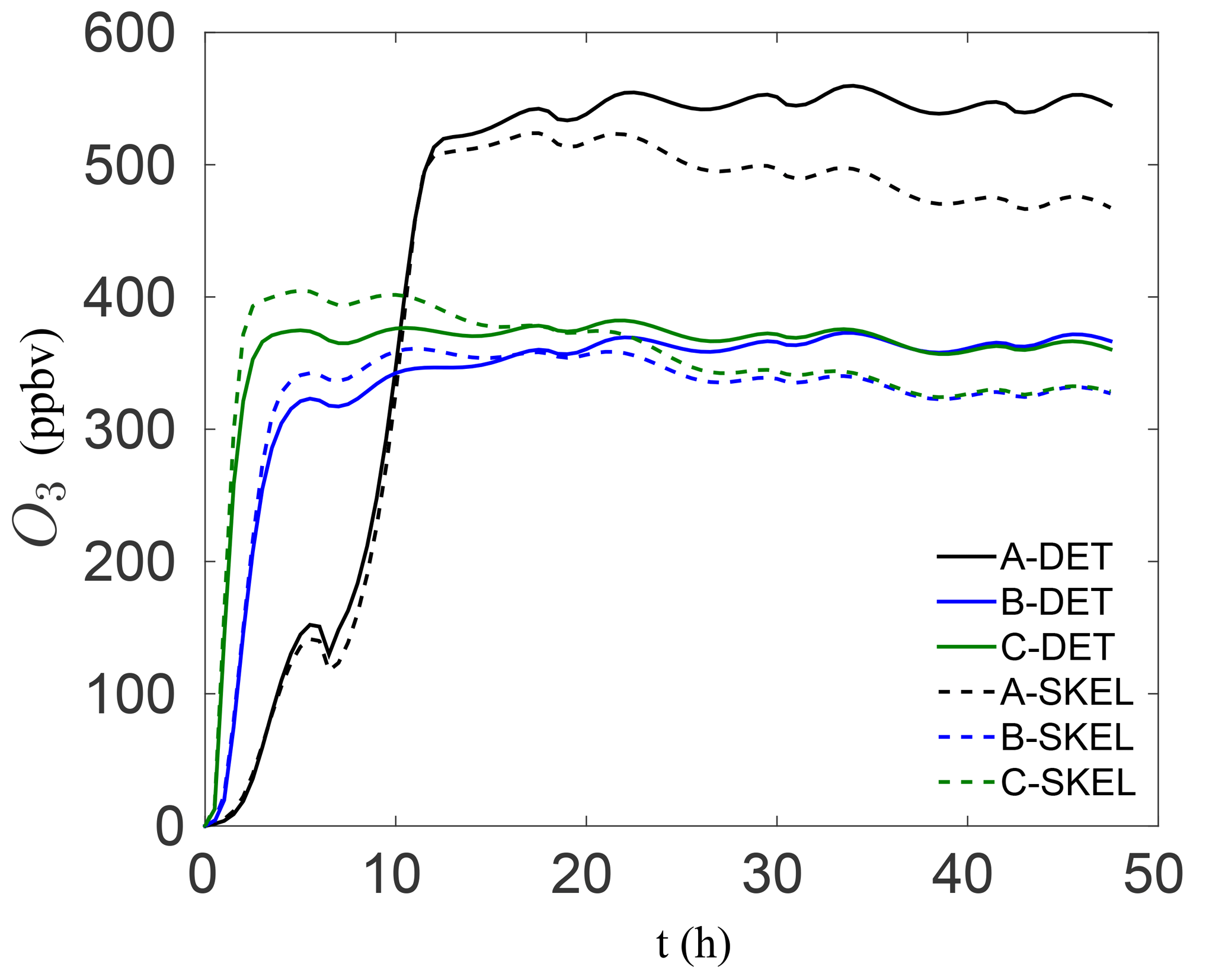
In order to visualize the errors in the ozone mixing ratio more clearly, Fig. 4 shows the solution profiles for scenarios A–C for the 48 h simulations, using the detailed and worst performing skeletal mechanism (which has 54 species). It is clear that the agreement with the detailed mechanism is very good for all six scenarios. In the isoprene scenarios D–F, similarly good results were obtained, although these results are not presented here. It is also important to note that the agreement is particularly good both early in the simulation and at later times for the box model problem. In a forecasting simulation, the situation is somewhat different. Typical time steps used in forecasting simulations are of the order of minutes, and a new initial-value problem is solved at every time step for the species mixing ratios, using the previous time step mixing ratios as the new initial condition. Furthermore, an operator splitting approach is used in the majority of codes for integrating the species mixing ratios, and this process is equivalent to filtering/smoothing the mixing ratio fields, which reduces the stiffness of the system. From this point of view, integration in forecasting codes is less stringent than integration in box model runs. In this sense, the skeletal mechanism need only be accurate enough over the integration time step, before the next initial-value problem is solved.

Figure 4Detailed and skeletal (N_sp=54) ozone profiles for cases A–C.

Download

It is also important to note that the skeletal mechanism was developed with relatively polluted conditions in mind, for predicting ozone, which explains the relatively large VOC∕NO_x ratios used for the reduction in Table 1. However, the method is general and can be tailored for modelling conditions of specific interest, e.g., low VOC∕NO_x conditions. In order to examine the performance of the smallest skeletal mechanism for such conditions, additional box model runs were conducted for significantly lower VOC∕NO_x ratios. In particular, the NO and NO₂ mixing ratios in Table 1 were increased by a factor of 6 for each species, leading to initial conditions with VOC∕NO_x ratios of 0.7, 1.8, and 3.2 for modified scenarios A^′–C^′, respectively. The results for the worst-performing skeletal mechanism (which has 54 species) are shown in Fig. 5. The agreement with the detailed chemical mechanism is particularly good for all three cases, both at early times and for longer times. Even though the chemistry for low VOC∕NO_x conditions is somewhat different, the results in Fig. 5 indicate that the reduction process is not as sensitive to the VOC∕NO_x ratio – the most important parameter was instead found to be variation in sunlight intensity due to the activation/deactivation of photosensitive reactions.

Figure 5Detailed and skeletal (N_sp=54) ozone profiles for modified high-NO_x (×6) cases A^′–C^′.

Download

The results of the previous section constitute an a priori validation. In an actual simulation, the photolysis rates and the species mixing ratios due to the effects of advection, diffusion, and so on, can be substantially different from the conditions in a box model. As a result, the species rates will also differ which affects the reduction process. The aim of this section is to examine the performance of the skeletal mechanism generated in the previous section, by implementing it in an actual atmospheric-chemistry simulation, and comparing it with results using the detailed chemical mechanism.

4.1 WRF-Chem simulation set-up

The Weather Research and Forecasting system with Chemistry (WRF-Chem/version 3.9.1.1) was employed in this work. WRF-Chem, which has been jointly developed by several research institutes (https://www2.acd.ucar.edu/wrf-chem, last access: 1 March 2018), is a state-of-the art, open source, limited-area atmospheric model, featuring a highly parallelized code. WRF-Chem is used for both research applications and for operational numerical weather and air-quality predictions, and is an online, fully coupled model, which integrates and calculates meteorology, gas-phase chemistry, and aerosols simultaneously (Grell et al., 2005). WRF-Chem utilizes the Advanced Research WRF (ARW) solver (Skamarock et al., 2005), where the transformation, mixing-phase, and transport of chemical species and aerosols, are calculated following the same prognostic equations, time step, and spatial configuration with the meteorology, physics, and other transport constituents of the ARW dynamical core.

In this study, the model is configured over a single domain using the lat–lon geographical projection, with about 0.15^∘ (∼16 km) horizontal grid spacing, and a domain of 165 (E–W) by 165 (N–S) grid points as shown in Fig. 6. Thirty vertical model levels were used, which correspond to a maximum height of about 20 km (∼50 hPa). Owing to its modular design, WRF-Chem provides several choices of chemical mechanisms and physics parameterizations. In this study, RACM is used for the gas-phase chemistry (Geiger et al., 2003; Stockwell et al., 1997b), and KPP is used for the integration of the species mixing ratios. The full RACM mechanism as implemented in WRF-Chem includes 75 species and 237 reactions. Table 3 summarizes the major model features and physical parameterizations as used in the simulations.

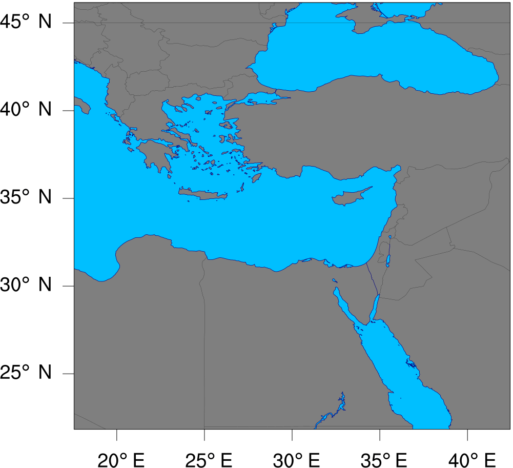
Figure 6The geographic domain utilized during the WRF-Chem simulations conducted in this study. The domain extends between 17.6 and 42.4^∘ E in the longitudinal direction, and between 21.9 and 46.1^∘ N in the latitudinal direction.

Download

(Tewari et al., 2004)(Hong et al., 2004)(Paulson, 1970; Webb, 1970)(Iacono et al., 2008)(Iacono et al., 2008)(Hong et al., 2006)(Grell and Dévényi, 2002)(Stockwell et al., 1997b)(Wild et al., 2000)

Table 3Settings and physical parameterization schemes selected during the WRF-Chem simulations.

Download Print Version | Download XLSX

The meteorological fields were forced by initial and lateral boundary conditions obtained from the National Centers for the Environmental Prediction/Global Forecast System (NCEP/GFS) at a spatial resolution of 0.25^∘, and updated at 3-hour intervals. MODIS-based geo-terrestrial data, including land categories, soil types, and terrain heights, were used. Our initial aim was to examine ozone mixing ratio predictions between the detailed mechanism and the skeletal mechanism using DRGEP, without the influence of any external source terms. Modelling emissions is a challenge on its own, and emissions inventories contain many uncertainties. Furthermore, these inventories always have inter-dependencies with the resolution of the mesh, the time step used, the chemical mechanism used, speciation profiling etc. This introduces uncertainties in evaluating the performance of the skeletal mechanism – including emissions would hinder the process of determining whether any errors are a result of the reduction process or a result of uncertainties in the emissions inventories. Thus, excluding emissions (at this stage) gives a clearer picture as to the effect of transport terms alone on the spatio-temporal distribution of ozone. In order to do that, anthropogenic/biogenic emissions were not utilized, and no chemical initial and boundary conditions were applied to the chemistry fields. For the latter, the model used idealized climatologically based values to initialize the chemical species instead. Further details of the initialization are given in the WRF-Chem user guide (WRF-Chem, 2017).

For the purposes of this study, two separate simulations were conducted for the period from 12 to 28 July 2017, a time of year during which ozone photochemistry is particularly active in this region. The first 5 days of the model output are considered as model spin-up time, and were excluded from our analysis. The model instantaneous, grid-cell averaged mixing ratios, were set to be written out (at the beginning of) every hour. The first simulation, used the complete (unmodified) RACM mechanism as implemented in the WRF-Chem package, while the second simulation utilized the skeletal (via DRGEP algorithm) mechanism. For a fair comparison between the two simulations, both set-ups shared the same namelist, which is included in the Supplement.

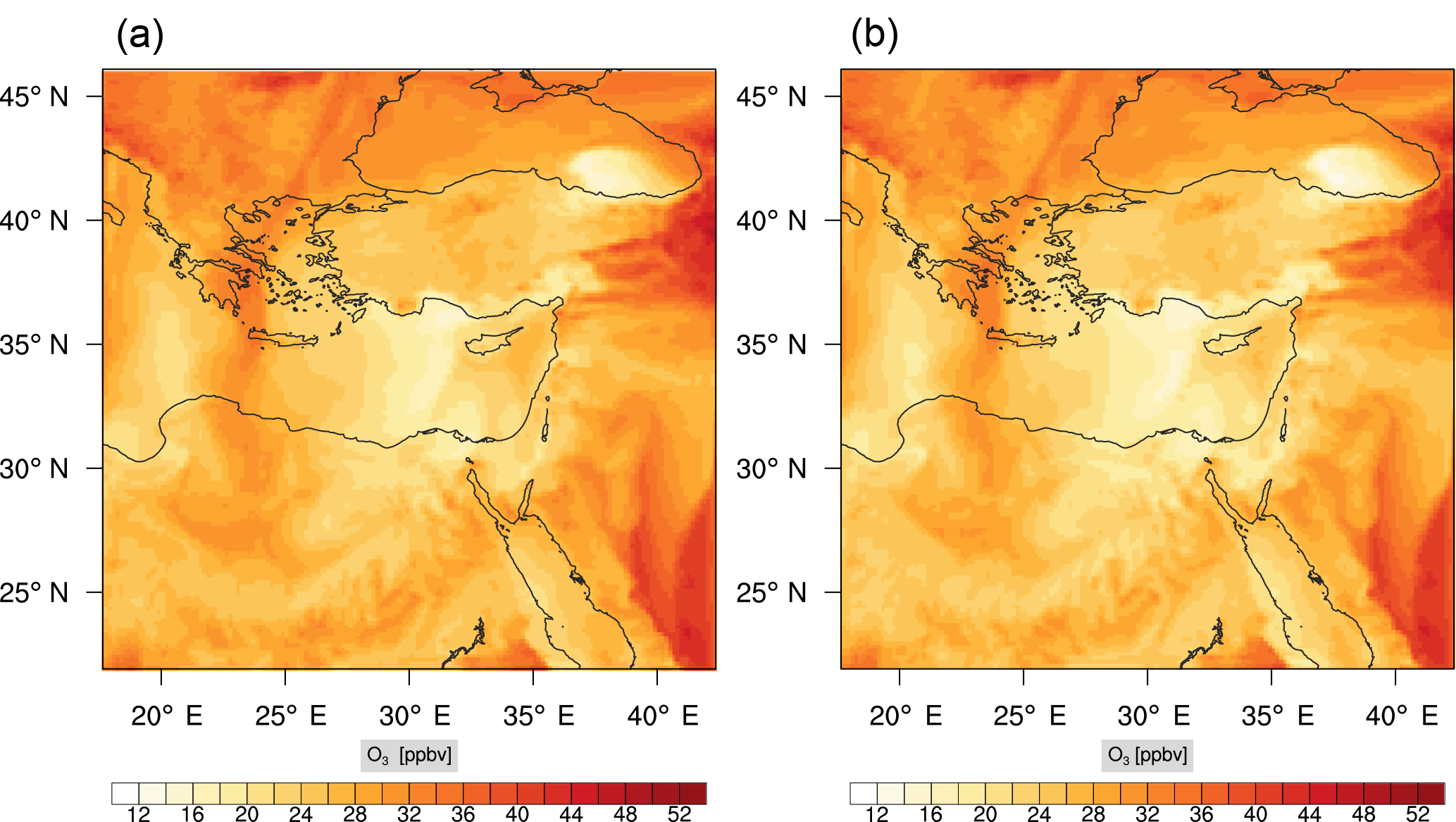
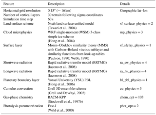
Figure 7Instantaneous comparison of the ozone spatial mixing ratio, averaged over the first nine vertical layers, using the full mechanism (a) and the skeletal mechanism (b).

Download

Figure 8(a) The volume-weighted average of the absolute percentage difference between the full and skeletal mechanisms, e^′(t), for the ozone mixing ratio. (b) The spatial distribution of the absolute percentage difference between the reduced and full mechanisms, with respect to the full mechanism, for the ozone mixing ratio when e^′(t) is maximum.

Download

The implementation of a new chemical mechanism in WRF-Chem is a rather tedious process. This includes creating new reaction and species files, compiling KPP with the new mechanism, and writing new mechanism-specific driver and initialization routines. A work-around, is to modify the existing chemical mechanism file (in this case RACM) instead, so that it accounts for the reduced chemistry. This simple method implies that driver routines do not need to be rewritten, calls to subroutines do not need to change to account for the reduction in species, and so on. This is achieved by setting dummy reactions for all species which are removed in the skeletal mechanism. The corresponding KPP reactions in the skeletal mechanism, are included in the Supplement. From a computational perspective, the skeletal mechanism was found to be more efficient than the detailed mechanism, as expected: on 40 MPI processes, the wall-clock times using the detailed and skeletal mechanisms were 959 and 730 min, respectively. This translates to an overall gain in CPU time of 24.6 %.

This speed-up is of the same order of magnitude as in the box model runs. However due to the implementation of the skeletal mechanism in WRF-Chem (all species kept), this speed-up does not include overheads. If a new mechanism were to be written (with fewer number of species), and all relevant subroutine calls suitably modified in order to include only the species in the skeletal mechanism, an even further gain in speed-up would be expected from simulation overheads (input/output, calls to subroutines etc.).

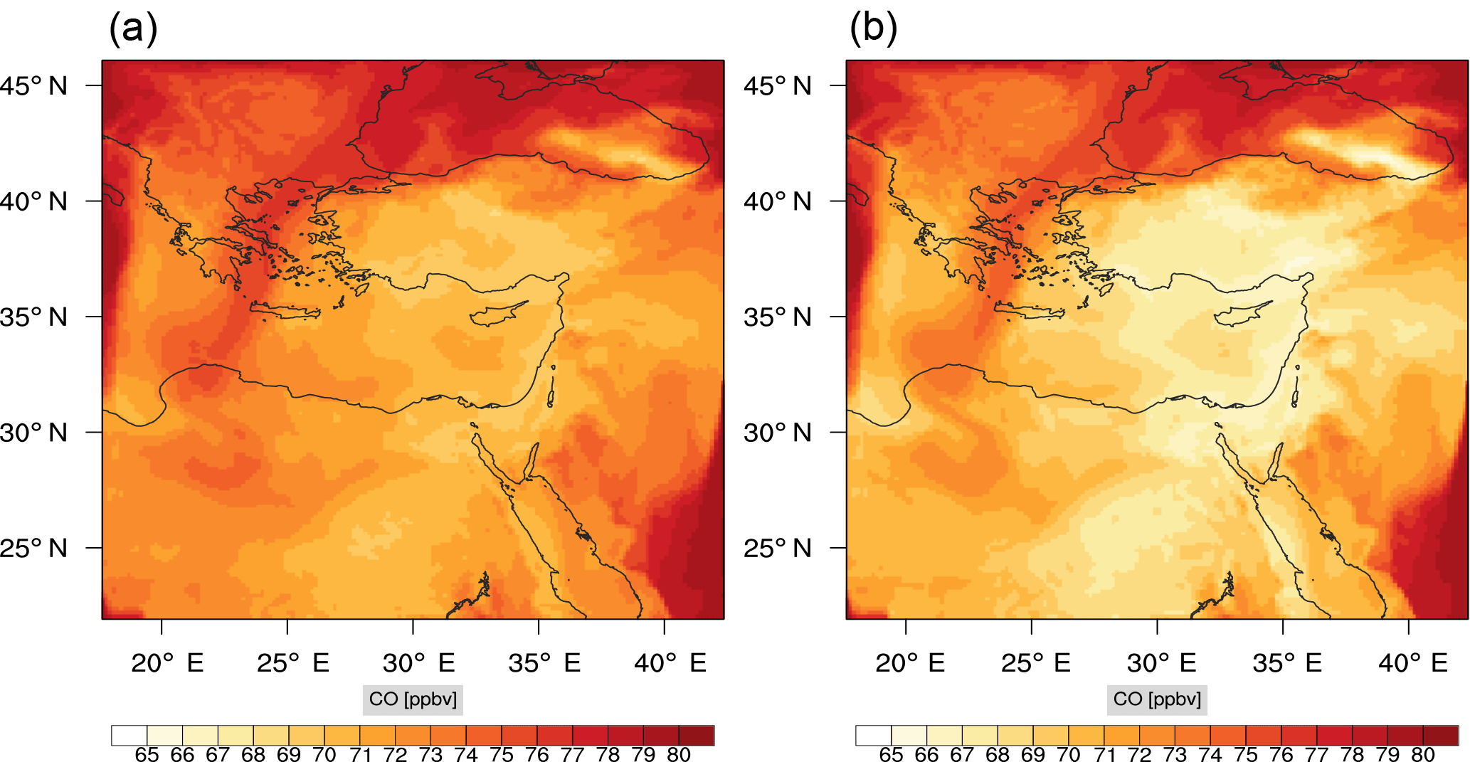
Figure 9Instantaneous comparison of the carbon monoxide spatial mixing ratio, averaged over the first nine vertical layers, using the full mechanism (a) and the skeletal mechanism (b).

Download

Figure 10(a) The volume-weighted average of the absolute percentage difference between the full and skeletal mechanisms, e^′(t), for the carbon monoxide mixing ratio. (b) The spatial distribution of the absolute percentage difference between the reduced and the full mechanisms, with respect to the full mechanism, for the CO mixing ratio when e^′(t) is maximum.

Download

4.3 Lower troposphere

Figure 7 shows a direct comparison between the ozone mixing ratios as predicted using the full mechanism (left) and the skeletal mechanism (right). The instance depicted, corresponds to the case of maximum error (e^′(t)). From visual inspection alone, it is clear that there is very good agreement for the spatial ozone concentration prediction using the skeletal mechanism.

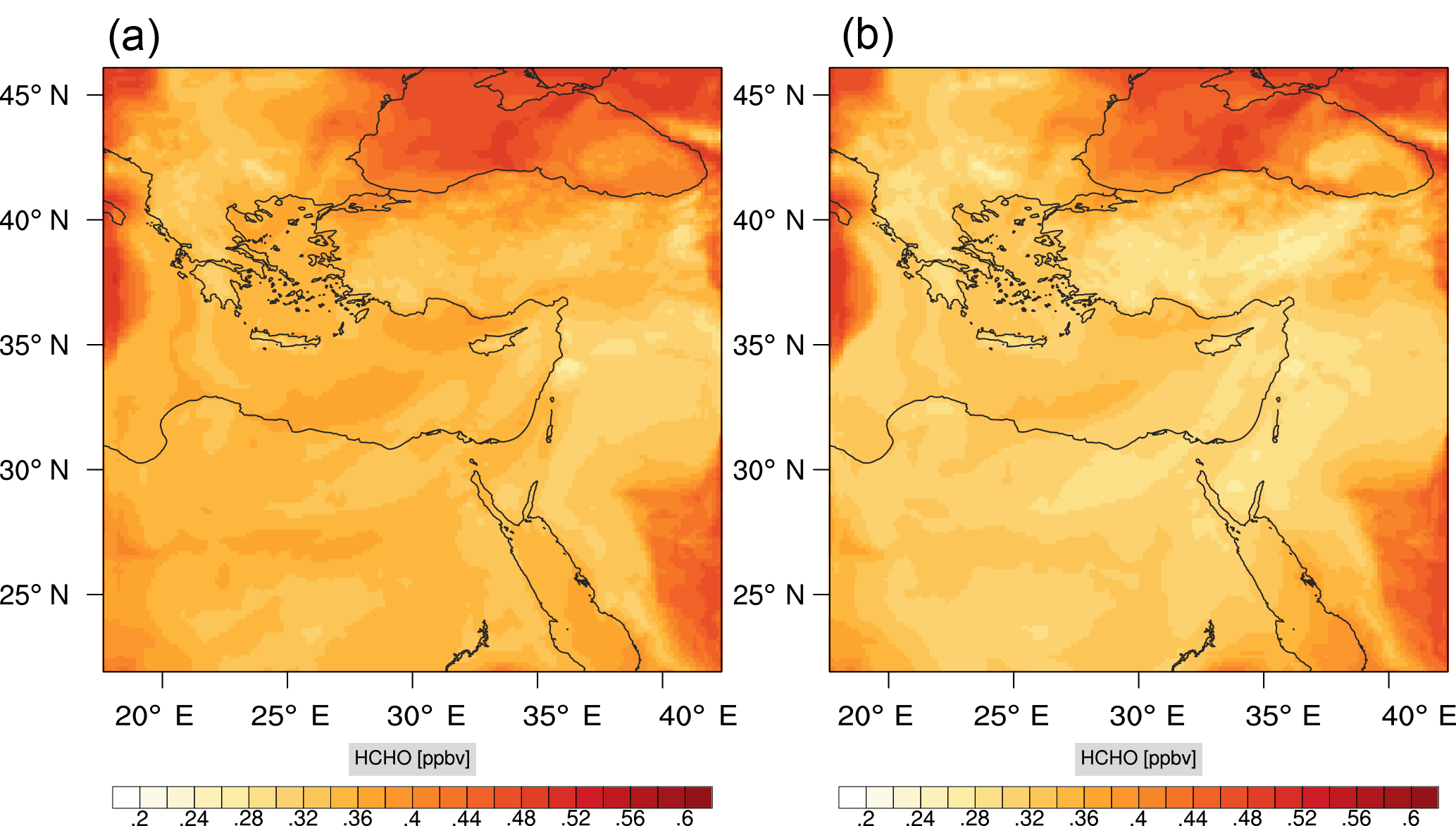
Figure 11Instantaneous comparison of the formaldehyde spatial mixing ratio, averaged over the first nine vertical layers, using the full mechanism (a) and the skeletal mechanism (b).

Download

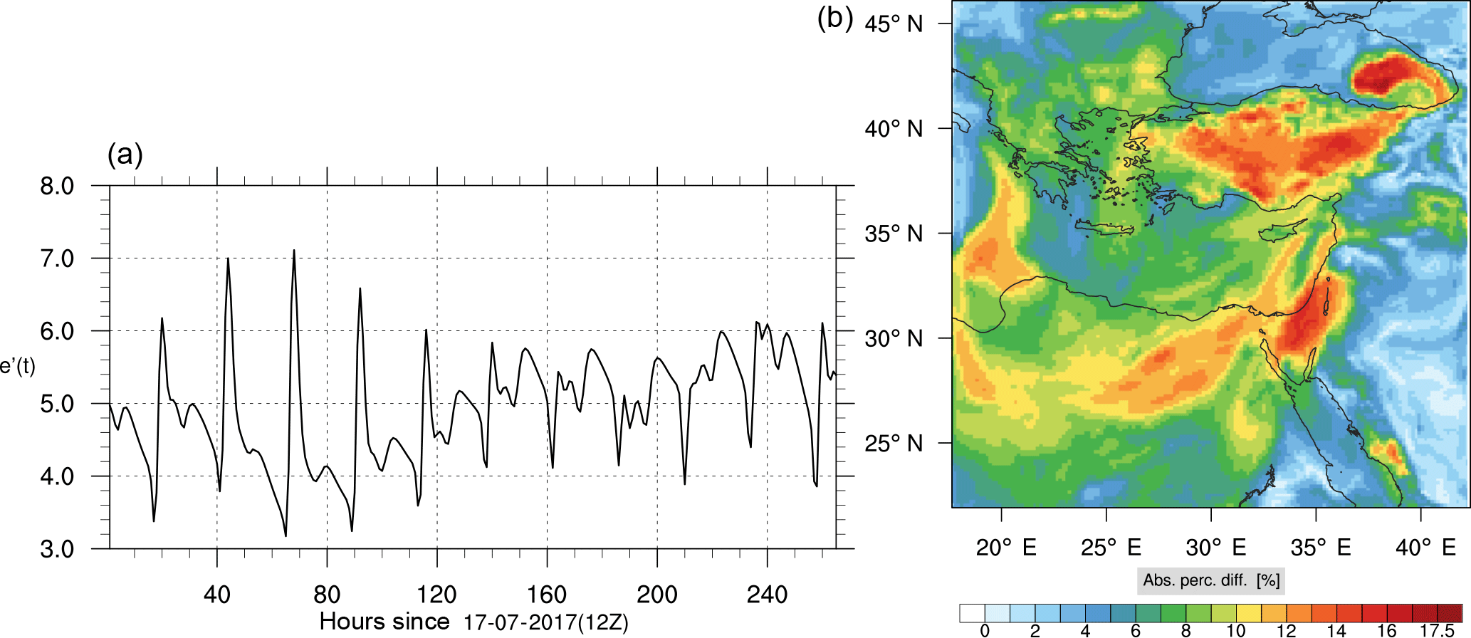
Figure 12(a) The volume-weighted average of the absolute percentage difference between the full and skeletal mechanisms, e^′(t), for the formaldehyde mixing ratio. (b) The spatial distribution of the absolute percentage difference between the reduced and the full mechanisms, with respect to the full mechanism, for the formaldehyde mixing ratio when e^′(t) is maximum.

Download

The corresponding error for the ozone mixing ratio field is depicted in Fig. 8a. Over the 265 time steps (hours) included in the analysis, it is found that e^′ varies between 2.52 % and 4.21 %. These small errors confirm the good agreement observed for the instantaneous ozone predictions shown in Fig. 7. Figure  8b shows the distribution of error, averaged in the vertical layers only, for the time instance of maximum, e^′, i.e., at 100 h. This helps to elucidate the actual spatial distribution of the error in terms of latitude and longitude. The error distribution is also within reasonable bounds at this instance, not exceeding 10 %. Note, that this distribution applies at the instance of maximum volume-averaged error as calculated using Eq. (10). This error is actually transported during the simulation, i.e., is not specific to a particular region.

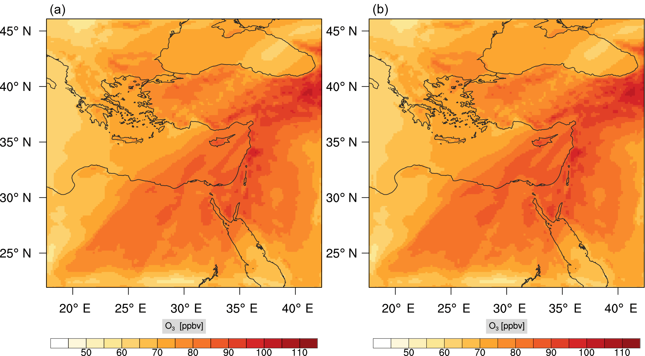
Figure 13Instantaneous comparison of the ozone spatial mixing ratio, averaged over the vertical layers 10–22, using the full mechanism (a) and the skeletal mechanism (b).

Download

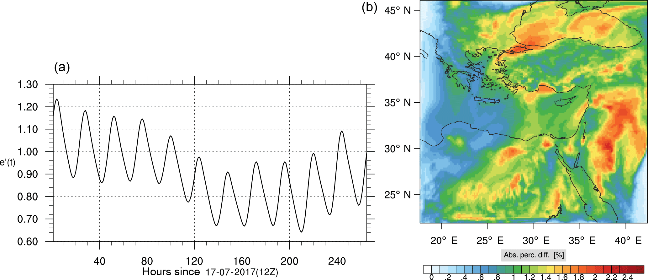
Figure 14(a) The volume-weighted average of the absolute percentage difference between the full and skeletal mechanisms, e^′(t), for the ozone mixing ratio. (b) The spatial distribution of the absolute percentage difference between the reduced and the full mechanisms, with respect to the full mechanism, for the ozone mixing ratio when e^′(t) is maximum.

Download

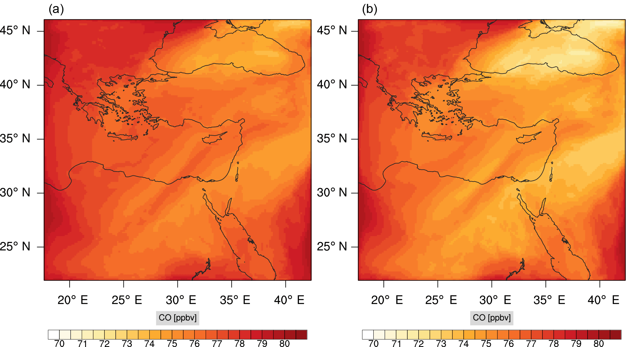
Figure 15Instantaneous comparison of the carbon monoxide spatial mixing ratio, averaged over the vertical layers 10–22, using the full mechanism (a) and skeletal mechanism (b).

Download

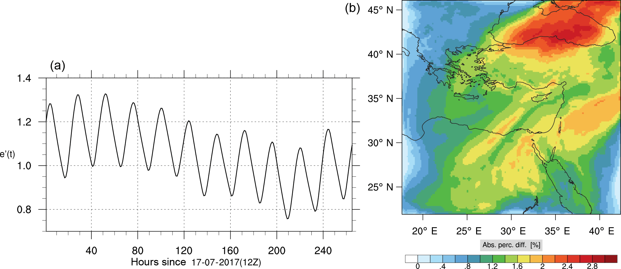
Figure 16(a) The volume-weighted average of the absolute percentage difference between the full and skeletal mechanisms, e^′(t), for the carbon monoxide mixing ratio. (b) The spatial distribution of the absolute percentage difference between the reduced and the full mechanisms, with respect to the full mechanism, for the CO mixing ratio when e^′(t) is maximum.

Download

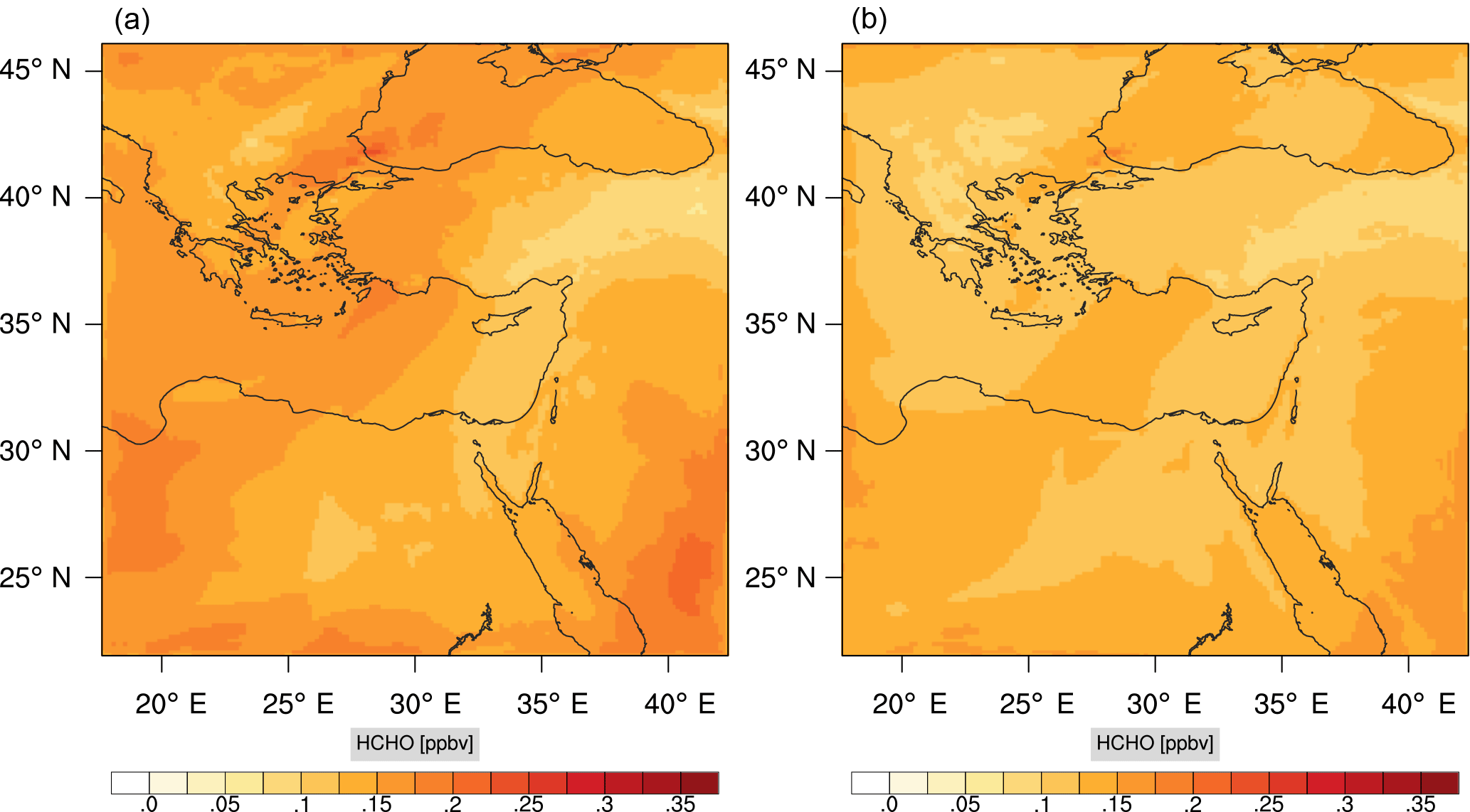
Figure 17Instantaneous comparison of the formaldehyde spatial mixing ratio, averaged over the vertical layers 10–22, using the full mechanism (a) and skeletal mechanism (b).

Download

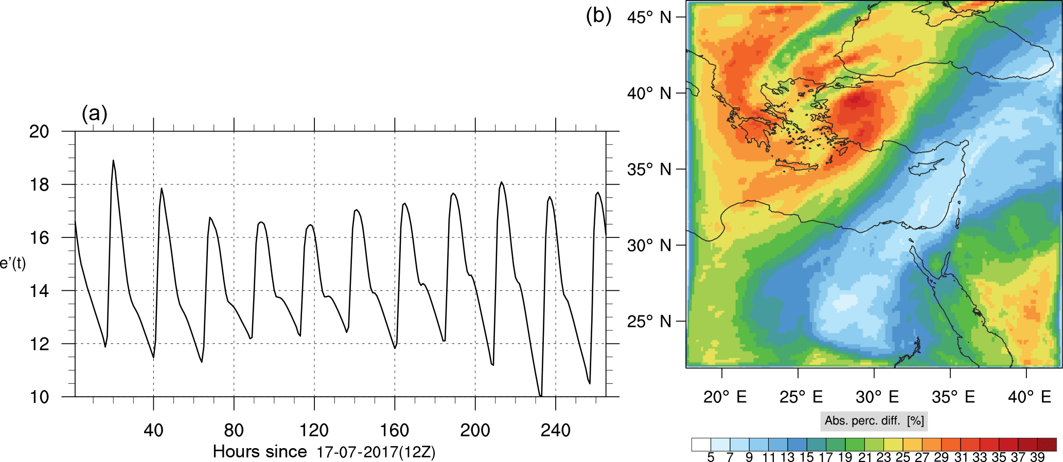
Figure 18(a) The volume-weighted average of the absolute percentage difference between the full and skeletal mechanisms, e^′(t), for the formaldehyde mixing ratio. (b) The spatial distribution of the absolute percentage difference between the reduced and the full mechanisms, with respect to the full mechanism, for the formaldehyde mixing ratio when e^′(t) is maximum.

Download

Figures 9, 10 and 11, 12 show the corresponding results for carbon monoxide which is a slow reacting species, and formaldehyde which is a relatively faster reacting species. Both of these species were not included as targets during the reduction; therefore, it is instructive to examine how their mixing ratio predictions compare to ozone which was the target species. Figures 9 and 10 show that the CO predictions are also in good agreement with relatively small percentage errors. The maximum volume-weighted error (e^′) for carbon monoxide during the simulation does not exceed 2.6 %. The instantaneous error averaged in the vertical layers only at the time of maximum e^′ also remains low as one may observed from Fig. 10b. The errors for formaldehyde in comparison are relatively large as one may observe from the results in Figs. 11 and 12. The maximum volume-weighted error is about 7 %, while the instantaneous error for the time of maximum e^′ is in the region of 20 % (Fig. 12b). Formaldehyde, which is an important intermediate species (Lelieveld et al., 2016), is involved in many oxidation reactions including a number of VOCs which explains the relatively larger errors. The same applies for the hydroxyl radical HO, which also displayed relatively large errors. In particular, for the subset mechanism including 54 species, higher alkanes such as HC3 and TOL (toluene) were identified as redundant species from the DRGEP. These species constitute an important HO consumption pathway, and excluding them leads to an overestimation of the HO mixing ratio. Much better results may be obtained by either reducing the OIC threshold (and including more species) or by including more targets during the reduction. However, both of these approaches lead to larger skeletal mechanisms and a reduction in speed-up; in other words, careful selection of the targets is required to obtain both an accurate and computationally fast mechanism.

The WRF-Chem package used for the numerical simulations is available from the National Center for Atmospheric Research (NCAR): https://www2.acom.ucar.edu/wrf-chem. The WRF-Chem namelist file, and the skeletal RACM mechanism are given as supplements. The code used for the DRGEP is attached as a Supplement and can also be obtained from the authors upon request.

The supplement related to this article is available online at: https://doi.org/10.5194/gmd-11-3391-2018-supplement.

ZN developed the DRGEP code, conducted the model-scenario (box model) simulations and developed the sub-set skeletal RACM. J-YC provided useful insight and guidance on the reduction process and code development. YP conducted the WRF-Chem simulations. JL and RS provided useful insight and comments. All authors co-wrote the manuscript.

The authors declare that they have no conflict of interest.