the Creative Commons Attribution 4.0 License.
the Creative Commons Attribution 4.0 License.
 | 24 Sep 2018
Verification of the mixed layer depth in the OceanMAPS operational forecast model for Austral autumn
Daniel Boettger
Robin Robertson
Gary B. Brassington
The ocean mixed layer depth is an important parameter describing the exchange of fluxes between the atmosphere and ocean. In ocean modelling a key factor in the accurate representation of the mixed layer is the parameterization of vertical mixing. An ideal opportunity to investigate the impact of different mixing schemes was provided when the Australian Bureau of Meteorology upgraded its operational ocean forecasting model, OceanMAPS to version 3.0. In terms of the mixed layer, the main difference between the old and new model versions was a change of vertical mixing scheme from that of Chen et al. (1994) to the General Ocean Turbulence Model.
The model estimates of the mixed layer depth were compared with those derived from Argo observations. Both versions of the model exhibited a deep bias in tropical latitudes and a shallow bias in the Southern Ocean, consistent with previous studies. The bias, however, was greatly reduced in version 3.0, and variance between model runs decreased. Additionally, model skill against climatology also improved significantly. Further analysis discounted changes to model resolution outside of the Australian region having a significant impact on these results, leaving the change in vertical mixing scheme as the main factor in the assessed improvements to mixed layer depth representation.


The mixed layer depth (MLD) is an important factor controlling the dynamics of air–sea interaction. As a proxy for the heat content of the ocean boundary layer, the MLD is critical in understanding the exchange of heat and moisture fluxes between the ocean and atmosphere. It also has biological consequences, with the depth of the mixed layer having a critical impact on primary productivity.
Because of its importance to air–sea interaction, an accurate representation of the MLD has been long considered a key dynamic of climate models. It is equally important in ocean general circulation models, particularly those used for operational ocean forecasting. The MLD plays a role in determining the likelihood of atmospheric convection over the ocean, has been linked to the development of severe weather in mid-latitude cyclones (Chambers et al., 2015), and is also a key factor in the development and intensity of tropical cyclones (Mao et al., 2000; Zhao and Chan, 2017).
The Ocean Modelling and Prediction System (OceanMAPS), the operational ocean forecasting system of the Australian Bureau of Meteorology (BoM), transitioned from version 2.2.1 to version 3.0 on 11 April 2016. While a number of changes were introduced in version 3.0, the most significant in terms of the MLD was a change in vertical mixing scheme from a modified version of Chen et al. (1994) scheme to the General Ocean Turbulence Model (GOTM; Burchard et al., 1999). During the transition period, both versions continued to run in parallel until July 2016, using the same observational data and atmospheric forcing. This provided an ideal opportunity to verify two versions of an operational forecasting system under essentially identical conditions. In this case, by isolating other factors, a verification of each model version also provided insights into the performance of each vertical mixing parameterization in an operational setting.
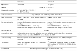
Table 1Details of the OceanMAPS versions compared in this study.
The purpose of this study is therefore (1) to quantify the impact of changes to the OceanMAPS forecasting system on the estimation of the MLD and (2) to assess the performance of the different vertical mixing parameterisations. These results will then inform the future development of OceanMAPS. Pertinent details of OceanMAPS, plus a description of the observational data used, are in Sect. 2. Section 3 details the method used for the calculation of the MLD, while the results of the analysis are reported in Sect. 4. Finally, the key results are discussed and expanded upon in Sect. 5.
2.1 The model
The BoM has run the OceanMAPS operational ocean forecasting system since 2007. The three main components of this system are the Ocean Forecasting Australian Model (OFAM), a data assimilation system, and atmospheric forcing from BoM's ACCESS-G model (Puri et al., 2013). While the atmospheric forcing remains unchanged between version 2.2.1 and version 3.0, changes to both OFAM and the data assimilation system that will impact the calculation of the MLD are highlighted below, with full details in Table 1.
The OFAM is a near-global (polar regions are excluded), eddy-resolving implementation of the Modular Ocean Model version 4p1 (MOM 4p1; Griffies, 2009). The latest version, OFAM3, is described in Oke et al. (2013). While the Chen et al. (1994) vertical mixing scheme had been used in OFAM2 (OceanMAPS version 2.2.1), the OFAM3 model implemented in OceanMAPS version 3.0 uses the General Ocean Turbulence Model (GOTM; Burchard et al., 1999). The Chen et al. (1994) scheme is a hybrid between a traditional bulk layer and the dynamical instability model of Price et al. (1986). It has been widely used in climate studies, particularly in tropical regions. Being initially formulated as an explicit MLD model, it was modified for use in the MOM by Power et al. (1995). The GOTM, conversely, is an attempt to unify many of the well-known turbulence closure schemes into a single model, with the characteristics of individual models replicated by changing the values of a number of constants.
In version 3.0, GOTM is configured as a k-ε scheme, with additional turbulent kinetic energy injection at the surface from wave breaking (Umlauf et al., 2003). While default parameters were used for most settings, the buoyancy production term was modified in order to stabilise turbulent kinetic energy advection. Following Rodi (1987), the rate of turbulent dissipation is calculated by
where 𝒟 is the sum of the viscous and turbulent transport terms, S and G are the rates of shear and buoyancy production, and cε∗ are model constants. The constant cε3 was defined such that if the buoyancy was positive (upwards), cε3 was equal to zero. This resulted in zero buoyancy production in cases where the buoyancy profile was convectively unstable. As G is generally 1 order of magnitude smaller than S, it only plays a significant role in turbulent mixing when G is relatively large and S relatively small. The impacts of these settings on the results are discussed further in Sect. 5.1.
While both versions of OFAM use a z* vertical coordinate system with identical resolution, the horizontal resolution does vary. OFAM2 employed a telescopic horizontal grid, with a 0.1∘ resolution around Australia (16∘ N to 75∘ S, 90 to 180∘ E) gradually decreasing outside of this region. In OFAM3, the horizontal resolution was fixed at 0.1∘ throughout the entire domain. While this can be expected to result in a marked improvement in the estimation of the MLD outside of the Australian region, within this region the impact on MLD will only be seen towards the boundaries, where the accuracy of incoming fluxes is improved. To isolate the effect of changing vertical mixing parameterisations, the analysis in this study is limited to the region where both models provided 0.1∘ resolution.
Version 2.2.1 ran four independent model cycles on consecutive days, with the spin-up period starting 9 days before the forecast start. Primarily designed to minimise over-fitting of the model fields to the available observations, this arrangement also enables the generation of a lagged time ensemble. In version 3.0, the number of model cycles was reduced to three, with the spin-up period extending to only 6 days. With initial verification of version 3.0 indicating a resultant significant decrease in sea surface temperature error (Bureau of Meteorology, 2017), it is probable that this will also have a positive impact on MLD estimation.
Other differences are listed in Table 1 and are expected to have a negligible impact on the relative skill of each model version to estimate the MLD. While the data assimilation software was upgraded in version 3.0, both versions still use the ensemble optimal interpolation method. The upgrade to the topography dataset has only made a significant difference for the continental shelf, over which the coverage of our observational dataset is negligible (Sect. 2.2). Furthermore, as neither version includes tidal forcing the impact of internal tide mixing is irrelevant for our comparison.
In summary, our interest is focussed on comparing the relative performance of the two versions to estimate the MLD, and in particular how the change in vertical mixing scheme has impacted this. While other changes between versions may also impact MLD estimation, the geographic constraints of our study minimise those influences, and the results that follow infer that the vertical mixing scheme accounts for the largest proportion of difference between model versions.
2.2 The dataset
Both the model and observational data were sourced from the Class 4 dataset (Ryan et al., 2015), developed through the GODAE OceanView programme in order to allow direct comparison of member organisation's ocean forecast model against a single Argo temperature and salinity dataset. While an Argo profile provides a near-instantaneous vertical profile, the standard OceanMAPS output consists of 24 h mean fields for all subsurface variables, hence any diurnal variation captured in the Argo observations will not be present in the model data. By limiting the analysis to depths where no diurnal variation can be expected, this limitation is overcome with minimal impact to the study (see Sect. 3).
Within the Class 4 dataset, the OceanMAPS temperature and salinity fields are interpolated (nearest-neighbour in the horizontal, linearly in the vertical) onto the Argo profiles out to +144 h, giving seven time steps for each model run. The dataset also includes a corresponding climatological temperature and salinity profile (Boyer et al., 2013), as well as a persistence forecast, where the model forecast is compared with a succession of the best estimate profiles from the previous six model runs.
Class 4 data for the period 11 April 2016 to 4 July 2016 were used, covering the operational overlap of OceanMAPS versions 2.2.1 and 3.0. Each profile was inspected to remove any unrealistic values or vertical gradients (Johnson et al., 2013), and profiles were only used in the analysis if a MLD was identified in the observed profile and in each model profile. The resultant quality controlled dataset provided 5316 individual profiles over the area of interest. Although the temporal extent of the dataset is relatively short, it covers an important transition period between the austral summer and winter seasons, during which the relative importance of heat and momentum fluxes in the ocean boundary layer is rapidly changing.
Conceptually, the MLD is well understood to represent the depth over which the mixing of surface fluxes has occurred. But the large variety of definitions used in the literature demonstrate the difficulty in accurately determining the MLD in all situations. Noting the relative paucity of in situ salinity observations, the majority of these identify the depth at which the temperature varies from the near-surface temperature by a certain amount, usually between 0.2 and 1.0 ∘C. As seawater density in the mid-latitudes and tropics is mostly proportional to temperature, this method generally provides a good estimate of the depth of the pycnocline and hence the depth to which surface mixing is limited. The minor dependence of density on salinity does, however, become important in some cases, particularly in the presence of a barrier layer or compensating layer.
Large amounts of precipitation, a common occurrence in equatorial regions, can result in a layer of cool, less saline water at the ocean surface overlaying a warmer, saltier layer. In this case, the surface isopycnal layer will be thicker than the isothermal layer, with the difference between the two termed the barrier layer (Lukas and Lindstrom, 1991). While a different mechanism is responsible, this type of vertical profile is also observed in high latitudes over winter months, where cool ocean surface temperatures overlay relatively warm, subsurface water (Kara et al., 2000). In the presence of a barrier layer, the temperature profile is a poor proxy for the depth of the mixed layer, and the density profile should be used.
Another surface mixed layer scenario is typified by a temperature and salinity profile that each have a negative gradient over the same depth, at such a rate that the density remains constant. Termed a compensating layer, this commonly occurs in regions with mean annual negative Ekman pumping (such as at the centre of subtropical gyres) and within subtropical convergence zones during winter (de Boyer Montégut et al., 2004). Although the density gradient is small in this instance, mixing is inhibited by the large temperature and salinity gradients present; consequently, the MLD is best defined as the top of the thermocline.
With salinity profiles available for both the model and observational datasets used here, the calculation of density is straightforward, and both a temperature and a density threshold can be used to account for the scenarios discussed above. Following de Boyer Montégut et al. (2004), the MLD is therefore defined as the first depth at which either of the following criteria are met:
Potential temperature, Θ, and potential density, ρΘ, are used to negate the depth dependence of the thermal expansion coefficient. The subscript “ref” denotes the value of each parameter at the reference depth, here set at a depth of 10 m in order to avoid diurnal variation that may be present in the observations but not reproduced in the daily mean model profiles. Temperature inversions are accounted for by using an absolute difference in Eq. (2). Using the shallowest depth derived by either the temperature or the density criterion ensures that the correct criteria is selected in both barrier layer and compensating layer scenarios.
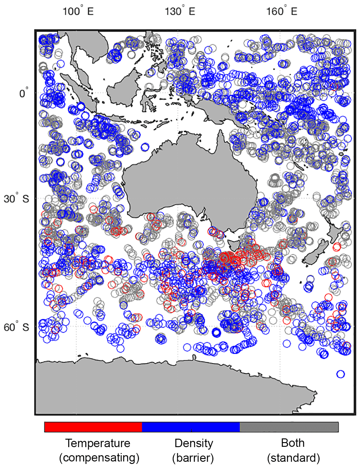
Figure 1Criteria used to identify the MLD for each Argo observation. Use of the density criterion implies the existence of a barrier layer, while use of the temperature criterion implies the existence of a compensated layer.
In 58 % of Argo profiles both the temperature and density criteria are met within 10 m or 5 % of the MLD (Fig. 1) and the locations where a single criterion has been used shows general agreement with previous studies. A compensating layer (i.e. where the temperature criterion is satisfied first) identified near Tasmania has been previously reported to exist during the winter months (de Boyer Montégut et al., 2004; Schiller and Ridgway, 2013), and locations of barrier layers (i.e. the density criterion is satisfied first) near the Equator and in the Southern Ocean correspond with regions of high precipitation and relatively cool sea surface temperatures, respectively. These results afford confidence that in most occasions the MLD is being correctly identified with this method.
4.1 Observed and forecast mixed layer depth
The MLD determined from the Argo observations (Fig. 2) matches the general trends for this season seen in previous studies (Carton et al., 2008; Kara et al., 2003; de Boyer Montégut et al., 2004; Schiller and Ridgway, 2013; Holte et al., 2016), and are in line with the conceptual model of seasonal mixed layer dynamics. In the tropics, the MLD is almost uniformly of the order of 20 m, with the small range of values indicated by the 5th and 95th percentiles shown at Fig. 2a. During the austral autumn, the Intertropical Convergence Zone shifts northwards from northern Australia towards the Equator, resulting in weak momentum and heat fluxes into the ocean. Deeper mixed layers are seen in the subtropical latitudes, particularly over the Coral Sea; here the south easterly trade wind regime generates increasingly strong winds and subsequently increases ocean mixing (Fig. 2b). Higher variability is also expected here due to the mesoscale structure of the coastal boundary currents. The deepest mixed layers are seen south of Australia, with values approaching 250 m around 50∘ S, where the Antarctic Circumpolar Current (ACC) is on average most active (Rintoul and Sokolov, 2001).
While the model results exhibit a similar spatial trend, the zonal mean of each model (Fig. 3a) identifies some distinct biases. Both models overpredict the depth of the mixed layer in the region 20–40∘ S, and under-predict the MLD around 45–65∘ S. A comparison between model versions shows that the magnitude of these biases has been reduced in version 3.0, while in the region 45–50∘ S the bias has disappeared. This can be attributed to a number of distinctly deeper estimations of the MLD in the region of the ACC to the south of Australia (Fig. 3b and c). In addition, the variability in the zonal mean between model forecast times (Fig. 3a) has decreased at all latitudes in version 3.0. This could be indicative of the changes to the forecast cycle implemented in version 3.0. By reducing the spin-up period and the number of individual ensemble members, the variability in the observational and atmospheric model forcing between each member is also reduced.

Figure 2(a) The zonal mean of the observed MLD (metres) derived from Class 4 Argo profiles over the study period; 90 % confidence intervals are shaded and the 5th and 95th percentiles are shown by the dotted lines. The number of profiles in each 5∘ bin is also indicated by the magenta line. (b) The individual MLD observations.
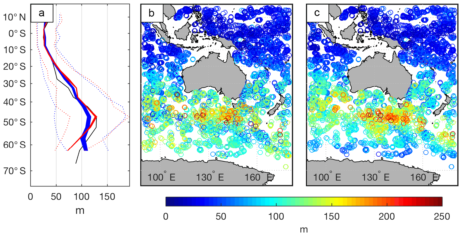
Figure 3(a) The zonal mean of the OceanMAPS versions 2.2.1 (blue) and 3.0 (red) MLD corresponding to Class 4 profiles over the study period. The range of values between forecast time steps (+0 h, +24 h, +48 h etc.) is indicated by the line thickness. The 5th and 95th percentiles for each model are shown by the dotted lines. The observed mean (from Fig. 2) is shown in black. The forecasts at model time +24 h are shown in (b) for version 2.2.1 and (c) for version 3.0.
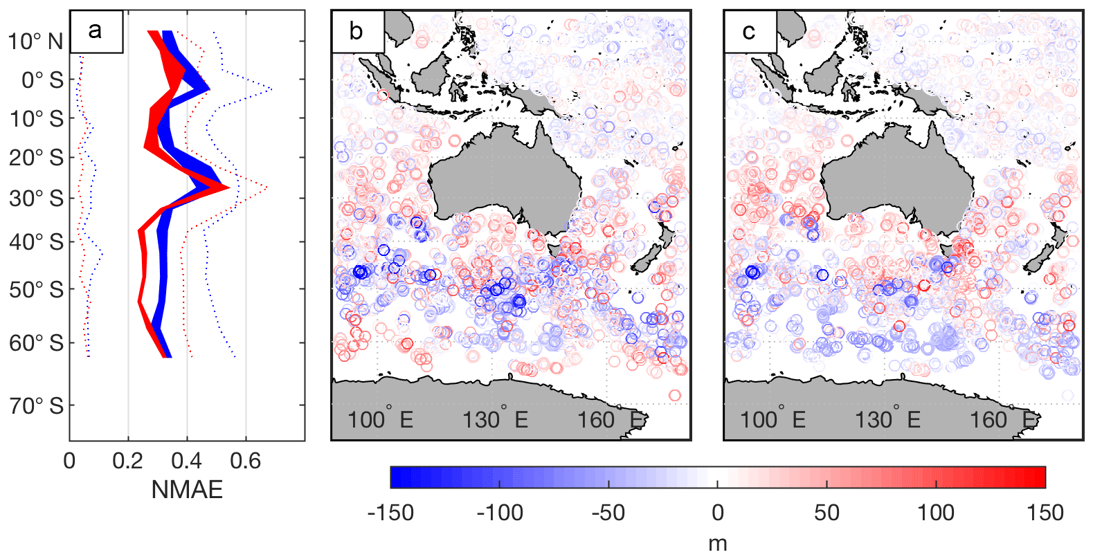
Figure 4(a) The normalised mean absolute error (NMAE) of the OceanMAPS 2.2.1 (blue) and 3.0 (red) MLD corresponding to Class 4 profiles over the study period. The range of values between forecast time steps (+0 h, +24 h, +48 h etc.) is indicated by the line thickness. The 5th and 95th percentiles for each model are shown by the dotted lines. The absolute error at model time +24 h are shown in (b) for version 2.2.1 and (c) for version 3.0.
4.2 Model error
To provide a more quantitative assessment of the differences between each model version, the magnitude of the difference between the observed and forecast MLD was calculated (Fig. 4). The regional bias previously discussed is again evident when the difference between each model and the Argo observations is plotted (Fig. 4b and c), with both models forecasting a deeper MLD in mid-latitudes and a shallower MLD south of Australia. As could be expected, the largest errors are seen in regions of high mesoscale activity, such as the East Australian Current, the Leeuwin Current, and the ACC.
The mean absolute error normalised by the meridional mean MLD (NMAE, Fig. 4a) highlights the differences between model versions, particularly in the Southern Ocean. Here, the NMAE has been reduced in version 3.0 by around 10 %, with a correspondingly large decrease in the spread of the error, indicated by the magnitude of the 95th percentile. North of 20∘ S the improvement in NMAE is more modest, but throughout the domain version 3.0 performs consistently better than version 2.2.1. The one exception to this trend, however, occurs around 30∘ S, where a spike in the NMAE of version 3.0 occurs. More in-depth analysis reveals that this can be attributed to the area between 90 and 100∘ E, where version 3.0 shows significantly larger errors than version 2.2.1 (Fig. 5, circled).
4.3 Model skill
A more quantitative measure of the forecasting ability of a model is the skill score (SS), here defined as the ratio of the root means square error (RMSE) of the model and a reference dataset (Ryan et al., 2015):
A positive skill score indicates that the model is a better predictor of the future state of the ocean then the reference dataset, while a negative skill score indicates the opposite. Commonly, climatology is used as a reference, with typical skill scores for operational ocean forecast models in the range 0.2 to 0.7 for parameters such as temperature, salinity and sea surface height (e.g. Divakaran et al., 2015; Ryan et al., 2015).

Figure 5The NMAE for OceanMAPS versions 2.2.1 (blue) and 3.0 (red), averaged over latitude and longitude bins. Each plot is scaled over 0–0.6. The number of profiles within each bin is indicated by the grey text. The area where version 2.2.1 performs better than version 3.0 discussed in Sect. 4.2 is circled.
The Class 4 dataset includes monthly temperature and salinity fields (Boyer et al., 2013) interpolated to the location and date of each Argo observation. Typically, the climatological skill score of a model decreases with forecast lead time (i.e. the model is less skilful looking further into the future), and this trend is seen in both versions of OceanMAPS (Fig. 6, light blue and red). To increase the number of profiles contained in each bin, here the data have been separated into tropical (16∘ N–20∘ S), mid-latitude (20–45∘ S) and high latitude (45–70∘ S) regions. Both models are more skilful than climatology within their data limits (+144 h), and within each region there is a distinct improvement in version 3.0 compared to 2.2.1.
The skill score also objectifies the relative difficulty of forecasting the state of the ocean in different regions. For example, in tropical waters there is relatively little spatial and temporal variation in the ocean boundary layer, and so it is more difficult for the model to make a significant improvement over the climatology. In the mid-latitudes, where mesoscale features unresolved by the climatology are dominant, larger skill scores are seen.
Model skill can also be measured against a persistence forecast, where each model time step is compared against the best estimate field for that model run. Persistence skill scores typically increase with increasing lead time; as time increases the current estimate of the ocean becomes a less useful estimate of its future state. Persistence skill scores for each version of OceanMAPS are difficult to interpret, with no clear trend for either model version (Fig. 6, dark blue and red). In the tropics for instance, the negative skill scores suggest that it is more often useful to rely on the persistence field then the actual forecast field. A possible cause for the irregular persistence results is the OceanMAPS forecast cycle, in which three (version 3.0) or four (version 2.2.1) independent model runs are initiated on consecutive days. Under this arrangement, the persistence scores are comparing forecast fields from different runs that have been forced with different observational datasets, introducing another layer of variability.
5.1 Southern Ocean response to model changes
The greatest improvements from version 2.2.1 to version 3.0, in terms of absolute error, occurred in the Southern Ocean and in particular around the ACC. One possible cause for this is the adoption of a global 0.1∘ horizontal grid in version 3.0 – in version 2.2.1 a telescopic grid was used, with 0.1∘ resolution around Australia and an expanding resolution elsewhere.
While our analysis has been constrained to the region where both model versions share a 0.1∘ horizontal grid, a strong zonal flow (such as the ACC) can advect any errors downstream. In this case, one may expect the version 2.2.1 results to show a relatively large error at the boundary of the highly resolved region (90∘ E) that gradually decreases downstream as the flow is resolved. Conversely, with a uniform horizontal resolution version 3.0 should exhibit a zonally uniform NMAE.
Examining Fig. 5, however, the zonal NMAE in the region of the ACC is generally uniform for both model versions, with the magnitude of the improvement between versions also uniform. This suggests that the change in global resolution has not had a significant effect on the estimation MLD. In the absence of other factors, it is likely that changing the mixing scheme to GOTM is primarily responsible for the improved results in this region.
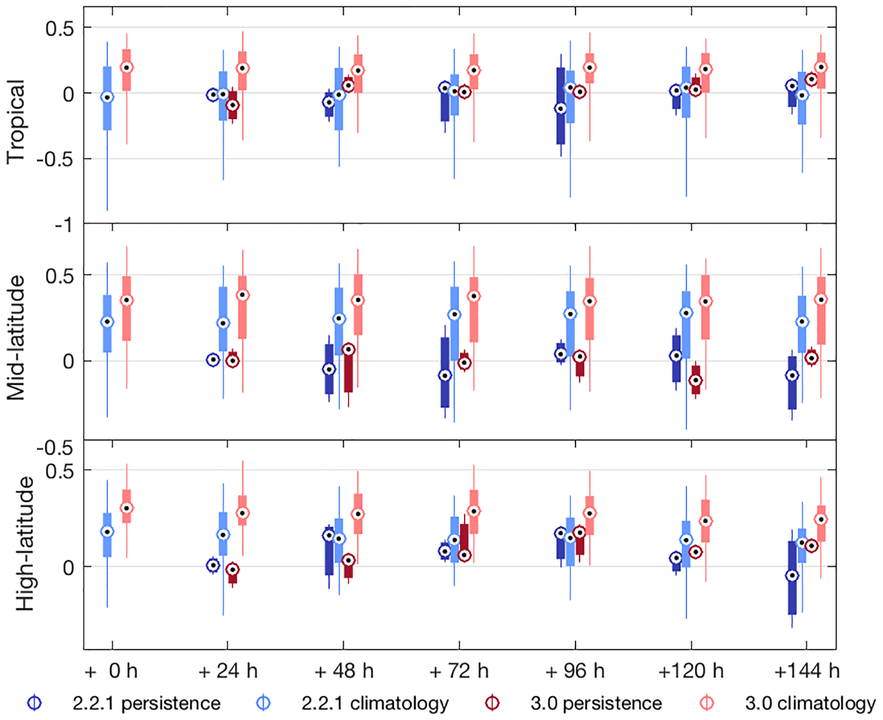
Figure 6Model climatology skill and persistence skill for OceanMAPS 2.2.1 (blue) and OceanMAPS 3.0 (red). The 5th and 95th percentiles are shown by the whiskers, while the middle quartiles are shown by the boxes. Data have been binned into tropical (16∘ N to 20∘ S), mid-latitude (20 to 45∘ S) and high-latitude (45 to 75∘ S) regions.
South of the ACC, in the region 55 to 65∘ S, the improvements seen in version 3.0 are less apparent. Here the zonal mean NMAE is of a similar magnitude for each model version (Fig. 4), with version 2.2.1 outperforming version 3.0 in some areas (Fig. 5). If a change of mixing scheme is responsible for the significant improvements seen elsewhere, then the reason that improvements are not seen here may lay in the distinct stratification profile common in high latitudes.
In version 3.0, buoyant production of turbulent kinetic energy, G, was limited to zero in instances where the buoyancy was positive (Sect. 2.1). The impacts of this on the MLD can be determined by examining the net surface fluxes of both buoyancy FG and shear FS. These are defined by
In Eq. (5), α and β are the thermal expansion and haline contraction coefficients, respectively; Q0 is the net surface heat flux; E and P the total evaporation and precipitation, respectively; and S0 the sea surface salinity. In Eq. (6), τ is the surface wind stress, κ the von Kármán constant and z set to the upper-most layer of the model (2.5 m).
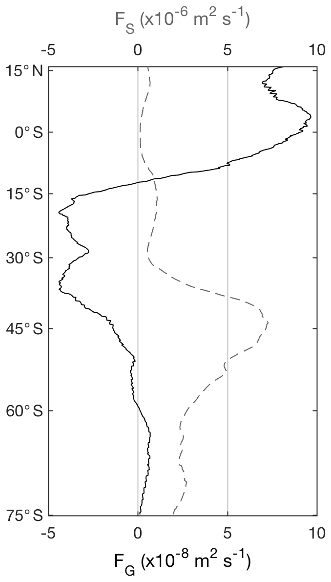
Figure 7The zonal mean surface buoyancy (FG, solid line) and shear (FS, dashed line) fluxes from OceanMAPS version 3.0. A positive (upwards) buoyancy flux tends to make the mixed layer unstable and promote mixing.
The zonal mean of the FG and FS from OceanMAPS version 3.0 are shown in Fig. 7. In the region of the ACC, FG is negative and stabilises the mixed layer, while the surface wind stress generates a large FS that drives turbulent mixing and generates a deep mixed layer. Conversely, south of 60∘ S, FG is positive and FS relatively small. Here, the G term in Eq. (1) would be significant, and the fact that this has been set to zero within version 3.0 will have a large impact on MLD estimates. This is the likely cause for the relatively poor performance of version 3.0 compared to version 2.2.1 seen in Fig. 5. A further conclusion that can be drawn from the Southern Ocean results is that version 3.0 significantly outperforms version 2.2.1 in shear-dominated mixing regions, whereas this improvement is negated in those regions where convective overturning is a significant factor.
5.2 Impact of the MLD definition on results
While the criteria used to identify the MLD are identical for both observation and model profiles, the individual characteristics of these datasets can result in varying levels of sensitivity to the same thresholds. For example, as the much greater vertical resolution of the Argo profiles allow finer features to be captured, it is possible that there will be some cases where a shallow temperature or density gradient unresolved in the model results in an apparent over-forecasting of the MLD. While a MLD definition based on simple temperature and density thresholds is effective for a typical mixed layer profile consisting of a single isothermal layer above the thermocline, more complex profiles can be incorrectly characterised.
To investigate what impact the magnitude of the temperature and salinity thresholds may have on results, a sensitivity study was conducted in which the thresholds were varied by up to ±50 % (Fig. 8). The impact is intuitive: an increase (decrease) in the magnitude of the thresholds increases (decreases) the estimated MLD. However, the effect is non-linear, with the observed MLD 12 % shallower when the threshold is 50 % smaller, but only 7 % deeper when the threshold is 50 % larger. Interestingly, OceanMAPS version 2.2.1 is more sensitive, and version 3.0 less sensitive, to threshold changes than the observations.
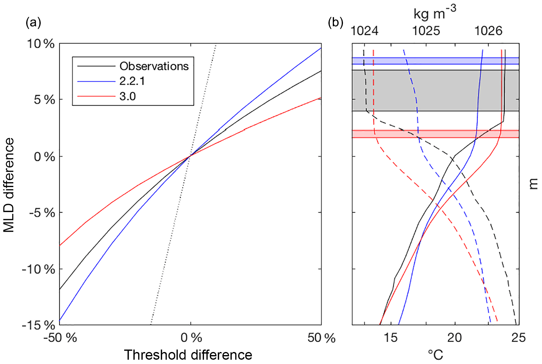
Figure 8(a) Mean difference in the calculated MLD as a result of varying the magnitude of the temperature and density thresholds. The dotted line indicates a slope of unity. (b) A typical Argo temperature (solid) and density (dashed) profile (location 28∘ S, 96∘ E), with the corresponding model estimates. The relative sensitivity of each dataset is indicated by the range of MLD estimates (shaded).

Figure 9The mean standard deviation of the potential temperature (top row) and potential density (bottom row) above the MLD, for observations (left column), OceanMAPS version 2.2.1 (centre column) and version 3.0 (right column).
This disparity between model versions can be explained by examining individual profiles, with a typical example shown in Fig. 8b. Here, the version 3.0 profile appears to capture the shape of the observed profile better than version 2.2.1. Critically, the version 3.0 profile is very well-mixed above the MLD, whereas the observations and the version 2.2.1 profile exhibit slight temperature and density gradients in this region, which have triggered the MLD thresholds. It is these gradients that control the sensitivity of the dataset to changes in the threshold magnitude.
The stratification of the layer above the MLD can be quantified using the standard deviation of the potential temperature and potential density (Fig. 9); a low value indicates a well-mixed layer while a high value indicates stratification. The observations reveal that the greatest amount of stratification above the MLD exists in the tropical regions north of 15∘ S, and that density exhibits a higher degree of spatial variability than temperature. A comparison with the model results explains the biases present in OceanMAPS; both versions produced a more well-mixed layer than observed in the mid-latitudes (where Fig. 3 indicated a deep bias) and a more stratified layer in the Southern Ocean (where Fig. 3 indicated a shallow bias). The differences in mixing between model versions is also evident here; while the GOTM mixing scheme used in version 3.0 generally produces a uniformly isothermal surface layer, the Chen et al. (1994) scheme used in version 2.2.1 often produces a more stratified layer that is more susceptible to changes in threshold magnitudes.
The difference between the sensitivity of the observations and each model version then raises the question: how does the choice of threshold affect the measurement of error in each model? The answer to this exhibits a strong spatial dependence. Decreasing (increasing) the magnitude of the thresholds decreases (increases) the NMAE north of 15∘ S, but increases (decreases) the NMAE south of this point (Fig. 10a, for threshold changes of ±50 %). While a more complex MLD definition incorporating spatially varying thresholds could better accommodate the observed meridional variation in mixed layer stratification, it may introduce other errors unless carefully implemented. Instead, this information is best used as a measure of the robustness of the error assessment of each model version. For example, increasing the thresholds would reduce the relative error between versions by approximately 5 % in the Southern Ocean, but would not change the relative performance of either version elsewhere. Overall, we conclude that the use of thresholds common to the existing literature offers the best compromise between accuracy and comparability with other studies.
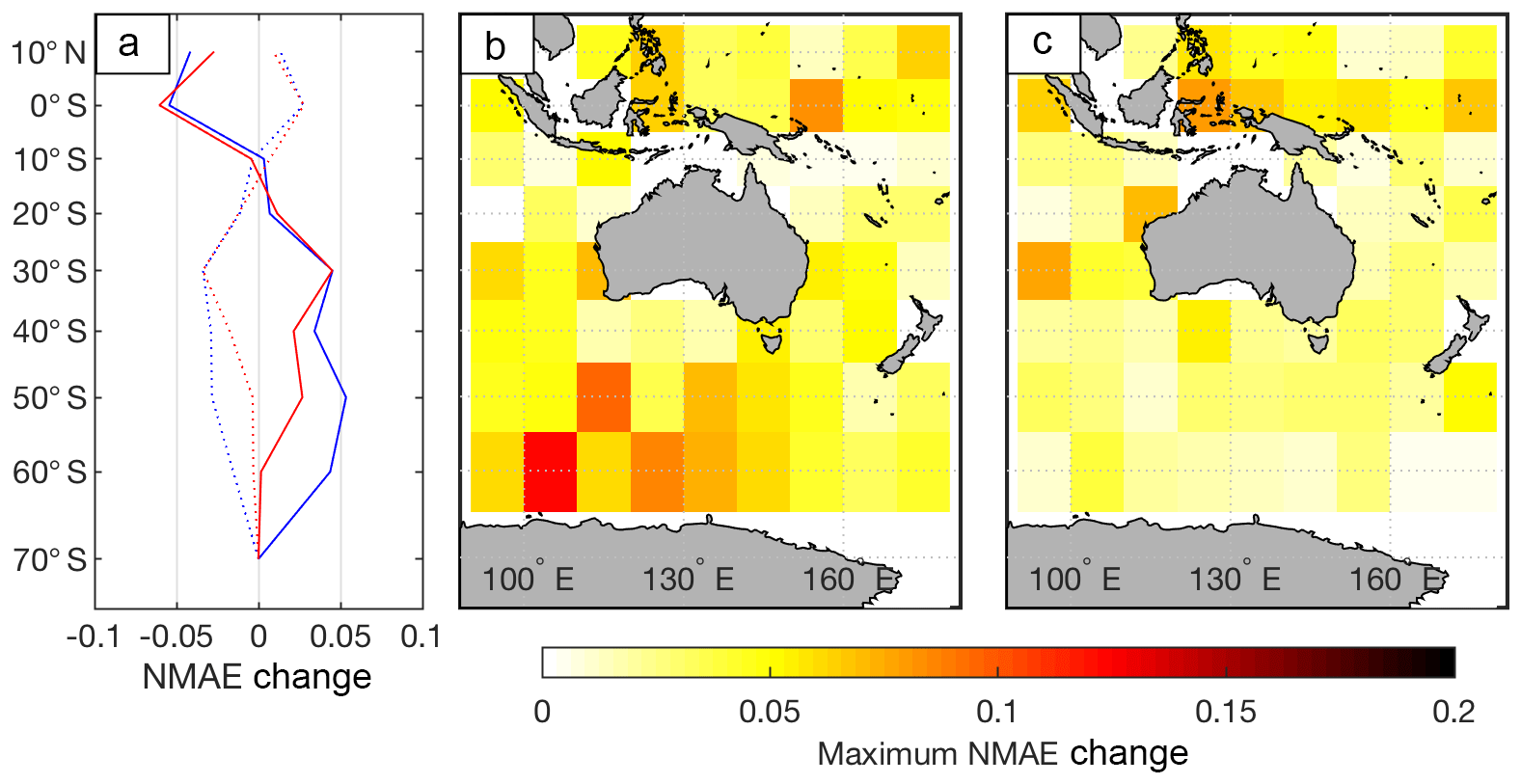
Figure 10(a) The change of the NMAE in MLD when the temperature and salinity thresholds are varied by +50 % (dotted) and −50 % (solid), for OceanMAPS version 2.2.1 (blue) and 3.0 (red). The maximum absolute change in NMAE recorded for a ±50 % change in thresholds is shown in latitude and longitude bins for version 2.2.1 (b) and 3.0 (c) are also shown.
One region where this general trend is not followed is the box 20–30 ∘ S, 90–100 ∘ E, where the version 3.0 NMAE is more sensitive to threshold changes than version 2.2.1. This is the same region that was highlighted in Sect. 4.2, where version 3.0 had a larger NMAE than version 2.2.1. Analysis of individual profiles in this region (e.g. Fig. 8) reveal a number of instances where the Argo and OceanMAPS version 2.2.1 profiles exhibit weak temperature and density gradients that trigger the MLD thresholds, whereas the OceanMAPS version 3.0 profile is well-mixed. In this case, the higher sensitivity shown in Fig. 10 for version 3.0 exists because, while changing the threshold has a small impact on the version 3.0 MLD, it has a large impact on the observed MLD that is subsequently expressed as “error”. Finally, some inferences may be drawn on the vertical mixing schemes in each model version; in areas where weak stratification is present within the mixed layer, the GOTM scheme in version 3.0 produces a deeper mixed layer than the Chen et al. (1994) scheme in version 2.2.1. This also suggests that the simplification of the buoyancy term in the GOTM implementation is not producing sufficient negative buoyancy to stabilise and stratify the mixed layer. However, in most cases the improvements to the shear-generated mixing still result in version 3.0 outperforming version 2.2.1.
The ability of version 2.2.1 and version 3.0 of the OceanMAPS operational ocean forecast model to accurately resolve the mixed layer depth (MLD) was quantified against a dataset of Argo temperature and salinity profiles. The analysis was limited to a region around Australia, where the major difference between model versions was a change in vertical mixing scheme.
In both model versions, a deep bias existed in the region 20–40∘ S and a shallow bias around 45–65∘ S. The magnitude of the bias was decreased in version 3.0 and was nearly erased in the region 45–50∘ S. A significant decrease in the variability of MLD estimates between model forecast runs was attributed to a shorter hindcast cycle in version 3.0. Version 3.0 also outperformed version 2.2.1 in all regions in terms of skill versus climatology. Skill versus persistence was also investigated but results were inconclusive; it is likely that additional sources of error are introduced into the persistence forecast included in the dataset by combining independent model cycles.
In nearly all areas, the magnitude of the normalised mean absolute error (NMAE) was reduced in version 3.0. The only exceptions were seen in the region 20–30∘ S, 90–100∘ E, where a weakly stratified mixed layer is common, and south of 55∘ S, where convective overturning is a significant mixing mechanism. These results suggest that while in most instances version 3.0 outperformed version 2.2.1, in situations where a positive (negative) buoyancy flux is a significant factor in making the mixed layer more (less) stable, the GOTM mixing scheme may generate excessive (insufficient) vertical mixing.
Having discounted other factors, it is most likely that significant improvements in the estimation of the MLD are mostly due to the change from the Chen et al. (1994) mixing scheme in version 2.2.1 to the GOTM in version 3.0. While limitations in the calculation of buoyancy production have been noted in version 3.0, the rectification of this issue is expected to deliver further improvements in mixed layer representation for future iterations of the OceanMAPS forecast system.
The Class 4 dataset and the analysis code used in this study are available at https://doi.org/10.4225/53/5ac71c59a5f49 (Boettger et al., 2018).
GBB suggested the study and provided the Class 4 dataset. DB implemented the methods and drafted the manuscript. GBB and RR supported the method development. All authors were involved in discussions throughout the project, and all authors commented on the paper.
The authors declare that they have no conflict of interest.
The authors thank the members of the BlueLink science team for their helpful
advice on the configuration of the OceanMAPS model.
This research was supported by an Australian Government Research Training Program (RTP) scholarship.
Edited by: Claire Levy
Reviewed by: two anonymous referees
Andreu-Burillo, I., Brassington, G., Oke, P., and Beggs, H.: Including a new data stream in the BLUElink Ocean Data Assimilation System, Aust. Meteorol. Ocean., 59, 77–96, 2010.
BODC: General Bathymetric Chart of the Oceans 2008 30 arcsecond topography, British Oceanographic Data Centre, 2008.
Boyer, T. P., Antonov, J. I., Baranova, O. K., Coleman, C., Garcia, H. E., Grodsky, A., Johnson, D. R., Locarnini, R. A., Mishonov, A. V., O'Brien, T. D., Paver, C. R., Reagan, J. R., Seidov, D., Smolyar, I. V., and Zweng, M. M.: World Ocean Database 2013, in: NOAA Atlas NESDIS 72, edited by: Levitus, S. and Mishonov, A., NODC, NOAA Printing Office, Silver Spring, MD, 2013.
Boettger, D., Robertson, R., and Brassington, G.: Class 4 Dataset – OceanMAPS version 2.2.1 and version 3.0, University of New South Wales, https://doi.org/10.4225/53/5ac71c59a5f49, 2018.
Burchard, H., Bolding, K., and Villarreal, M. R.: GOTM: a general ocean turbulence model. Theory, applications and test cases, European CommissionTech. Rep. EUR 18745 EN, 104, 1999.
Bureau of Meteorology: Operational Upgrade to OceanMAPS version 3 (BLUElink>Ocean Forecast System) – global ocean forecasting, 34, 2017.
Carton, J. A., Grodsky, S. A., and Liu, H.: Variability of the Oceanic Mixed Layer, 1960–2004, J. Climate, 21, 1029–1047, 2008.
Chambers, C., Brassington, G., Walsh, K., and Simmonds, I.: Sensitivity of the distribution of thunderstorms to sea surface temperatures in four Australian east coast lows, Meteorol. Atmos. Phys., 127, 499–517, 2015.
Chen, D., Rothstein, L., and Busalacchi, A.: A hybrid vertical mixing scheme and its application to tropical ocean models, J. Phys. Oceanogr., 24, 2156–2179, https://doi.org/10.1175/1520-0485(1994)024<2156:AHVMSA>2.0.CO, 1994.
Dai, A. and Trenberth, K.: Estimates of freshwater discharge from continents: Latitudinal and seasonal variations, J. Hydrometeorol., 3, 660–687, 2002.
de Boyer Montégut, C., Madec, G., Fischer, A. S., Lazar, A., and Iudicone, D.: Mixed layer depth over the global ocean: An examination of profile data and a profile-based climatology, J. Geophys. Res.-Oceans, 109, 1–20, 2004.
Griffies, S.: Elements of MOM 4p1, GFDL Ocean Group Technical Report No. 6, 32, 2009.
Holte, J., Gilson, J., Talley, L., and Roemmich, D.: Argo Mixed Layers, Oceanography/UCSD, S. I. o., Scripps Institution of Oceanography/UCSD 2016.
Divakaran, P., Brassington, G. B., Ryan, A. G., Regnier, C., Spindler, T., Mehra, A., Hernandez, F., Smith, G. C., Liu, Y., and Davidson, F.: GODAE OceanView Inter-comparison for the Australian Region, J. Oper. Oceanogr., 8, 112–126, 2015.
Johnson, D. R., Boyer, T. P., Garcia, H. E., Locarnini, R. A., Baranova, O. K., and Zweng, M. M.: World Ocean Database 2013 User's Manual, NODC, Silver Spring, MD, 172, 2013.
Kara, A. B., Rochford, P. A., and Hurlburt, H.: Mixed layer depth variability and barrier layer formation over the North Pacific Ocean, J. Geophys. Res.-Oceans, 105, 16783–16801, 2000.
Kara, A. B., Rochford, P. A., and Hurlburt, H. E.: Mixed layer depth variability over the global ocean, J. Geophys. Res.-Oceans, 108, https://doi.org/10.1029/2000JC000736, 2003.
Lukas, R. and Lindstrom, E.: The mixed layer of the western equatorial Pacific Ocean, J. Geophys. Res.-Oceans, 96, 3343–3357, 1991.
Mao, Q., Chang, S. W., and Pfeffer, R. L.: Influence of large-scale initial oceanic mixed layer depth on tropical cyclones, Mon. Weather Rev., 128, 4058–4070, 2000.
Oke, P. R., Brassington, G. B., Griffin, D. A., and Schiller, A.: The Bluelink ocean data assimilation system (BODAS), Ocean Modell., 21, 46–70, 2008.
Oke, P. R., Griffin, D. A., Schiller, A., Matear, R. J., Fiedler, R., Mansbridge, J., Lenton, A., Cahill, M., Chamberlain, M. A., and Ridgway, K.: Evaluation of a near-global eddy-resolving ocean model, Geosci. Model Dev., 6, 591–615, https://doi.org/10.5194/gmd-6-591-2013, 2013.
Power, S., Kleeman, R., Tseitkin, F., and Smith, N. R.: On a global version of the GFDL modular ocean model for ENSO studies, Melbourne, 18, 1995.
Price, J. F., Weller, R. A., and Pinkel, R.: Diurnal cycling: Observations and models of the upper ocean response to diurnal heating, cooling, and wind mixing, J. Geophys. Res.-Oceans, 91, 8411–8427, 1986.
Puri, K., Dietachmayer, G., Steinle, P., Dix, M., Rikus, L., Logan, L., Naughton, M., Tingwell, C., Xiao, Y., Barras, V., Bermous, I., Bowen, R., Deschamps, L., Franklin, C., Fraser, J., Glowacki, T., Harris, B., Lee, J., Le, T., Roff, G., Sulaiman, A., Sims, H., Sun, X., Sun, Z., Zhu, H., Chattopadhyay, M., and Engel, C.: Implementation of the initial ACCESS numerical weather prediction system, Aust. Meteorol. Ocean., 63, 265–284, 2013.
Rintoul, S. R. and Sokolov, S.: Baroclinic transport variability of the Antarctic Circumpolar Current south of Australia (WOCE repeat section SR3), J. Geophys. Res.-Oceans, 106, 2815–2832, 2001.
Rodi, W.: Examples of calculation methods for flow and mixing in stratified fluids, J. Geophys. Res.-Oceans, 92, 5305–5328, 1987.
Ryan, A. G., Regnier, C., Divakaran, P., Spindler, T., Mehra, A., Smith, G. C., Davidson, F., Hernandez, F., Maksymczuk, J., and Liu, Y.: GODAE OceanView Class 4 forecast verification framework: global ocean inter-comparison, J. Oper. Oceanogr., 8, s98–s111, 2015.
Sakov, P.: EnKF-C user guide. arXiv:1410.1233., arXiv preprint, 2014.
Schiller, A. and Ridgway, K. R.: Seasonal mixed-layer dynamics in an eddy-resolving ocean circulation model, J. Geophys. Res.-Oceans, 118, 3387–3405, 2013.
Smith, W. H. F. and Sandwell, D. T.: Global sea floor topography from satellite altimetry and ship depth soundings, Science, 277, 1956–1962, 1997.
Umlauf, L., Burchard, H., and Hutter, K.: Extending the k-omega turbulence model towards oceanic applications, Ocean Model., 5, 195–218, 2003.
Whiteway, T. G.: Australian bathymetry and topography grid, June 2009, Canberra, A.C.T., Australia: Geoscience Australia, Canberra, A.C.T., 2009.
Zhao, X. and Chan, J. C. L.: Changes in tropical cyclone intensity with translation speed and mixed-layer depth: idealized WRF-ROMS coupled model simulations, Q. J. Roy. Meteorol. Soc., 143, 152–163, 2017.