the Creative Commons Attribution 4.0 License.
the Creative Commons Attribution 4.0 License.
 | 27 Sep 2018
LCice 1.0 – a generalized Ice Sheet System Model coupler for LOVECLIM version 1.3: description, sensitivities, and validation with the Glacial Systems Model (GSM version D2017.aug17)
Taimaz Bahadory
Lev Tarasov
We have coupled an Earth system model of intermediate complexity (LOVECLIM) to the Glacial Systems Model (GSM) using the LCice 1.0 coupler. The coupling scheme is flexible enough to enable asynchronous coupling between any glacial cycle ice sheet model and (with some code work) any Earth system model of intermediate complexity (EMIC). This coupling includes a number of interactions between ice sheets and climate that are often neglected: dynamic meltwater runoff routing, novel downscaling for precipitation that corrects orographic forcing to the higher resolution ice sheet grid (“advective precipitation”), dynamic vertical temperature gradient, and ocean temperatures for sub-shelf melt. The sensitivity of the coupled model with respect to the selected parameterizations and coupling schemes is investigated. Each new coupling feature is shown to have a significant impact on ice sheet evolution.
An ensemble of runs is used to explore the behaviour of the coupled model over a set of 2000 parameter vectors using present-day (PD) initial and boundary conditions. The ensemble of coupled model runs is compared against PD reanalysis data for atmosphere (2 m temperature, precipitation, jet stream, and Rossby number of jet), ocean (sea ice and Atlantic Meridional Overturning Circulation – AMOC), and Northern Hemisphere ice sheet thickness and extent. The parameter vectors are then narrowed by rejecting model runs (1700 CE to present) with regional land ice volume changes beyond an acceptance range. The selected subset forms the basis for ongoing work to explore the spatial–temporal phase space of the last two glacial cycles.
- Article
(3517 KB) -
Supplement
(249 KB) - BibTeX
- EndNote


Transitions between glacial and interglacial states have been a periodic feature of the Earth's climate for the last few million years. The driver of these transitions is understood to be orbital forcing (Berger, 2014; Birch et al., 2016, 2017; Rind et al., 1989), with an important role for CO2 variations (Elison Timm et al., 2015; Ganopolski et al., 2016). Nevertheless, the role that climate feedbacks play in amplifying or inhibiting the responses to these forcings is not clear. Given available proxy data, how well do we know the progression of these glacial cycles? Is there more than one way each transition could have occurred? How sensitive were these glacial cycles to small perturbations in the external forcings (e.g., volcanic eruptions)? In order to address these questions, we need to understand the relative importance of different feedbacks between ice sheets and other aspects of the climate system. We can build such understanding by probing this phase space with physically based models that include the pertinent feedbacks on glacial timescales.
Temperature and net precipitation (the solid/liquid fraction thereof) encompass the main atmospheric impacts on ice sheets. Marginal ice sheet surface mass balance is very sensitive to the vertical temperature gradient. As indicated by the observations presented by Gardner et al. (2009), the vertical surface temperature gradient (“slope lapse rate”) can be significantly different from the free-air temperature lapse rate over the Greenland ice sheet. Furthermore, neither of these vertical temperature gradients are a priori appropriate for downscaling near surface temperatures to a higher horizontal resolution grid. The actual vertical gradient required is the one due to changing the surface topography in the climate model. However, most coupled model studies use a fixed vertical temperature gradient set to an approximate mean free-air lapse rate (usually between 5 and 7 K km−1) to downscale surface temperatures from coarse climate model grids (Glover, 1999; Flowers and Clarke, 2002; Thomas et al., 2003; Arnold et al., 2006; Bassford et al., 2006b, a; De Woul et al., 2006; Raper and Braithwaite, 2006). A somewhat more self-consistent approach regarding the atmospheric component of the climate model is provided by Roche et al. (2014). Their coupler extracts the vertical “along-slope surface temperature gradient” from the atmospheric model and uses it to downscale temperatures to the ice sheet model. They find this dynamic approach has significant impacts, especially over mountainous regions and Greenland.
Coarse grid climate models used in long time integrations can not resolve surface slopes on the generally much higher resolution ice sheet grids to which they are coupled. Given the strong impact of orographic forcing on precipitation, this can potentially introduce large errors in surface mass balance, especially near ice sheet margins and over rough topography. Therefore, standard bilinear interpolation schemes for downscaling precipitation to the ice sheet grid preserve these errors.
Ice sheets directly affect the atmosphere via changing land surface type (affecting albedo, surface roughness, and moisture fluxes) and changing topography. Upscaling of topography from the relatively high-resolution grids of ice sheet models to the course-resolution atmospheric grids (especially for fast glacial cycle context models) has a range of options between conserving peak heights and mean heights. There is no clear criteria for a “best” choice and the sensitivity to this choice is generally unclear.
Ice sheets primarily affect oceans directly through meltwater runoff, and changing ocean bathymetry and land mask (especially gateways). The effect of ice sheet runoff on the ocean, especially on the AMOC (Atlantic Meridional Overturning Circulation), has been the focus of many studies, such as Timmermann et al. (2003), Rahmstorf et al. (2005), Stouffer et al. (2006), Krebs and Timmermann (2007), Hu et al. (2008), Otto-Bliesner and Brady (2010), Kageyama et al. (2013), Xun et al. (2013), and Roberts et al. (2014). Their findings show that the modelled AMOC is a function of the models and the coupling procedures used, in addition to the initial and boundary conditions of the experiments. These experiments generally include prescribed freshwater discharge fluxes into the ocean, in part to isolate AMOC sensitivity to freshwater forcing. Therefore, the feedback of the resulting climate response on ice sheet discharge is absent.
The strongest direct impact of the oceans on ice sheets is submarine melt of tide water glaciers and sub-ice shelf melt. However, for continental scale coupled models, sub-shelf melt is either completely ignored (Ridley et al., 2005), or parameterized in a highly simplified way (e.g., Roche et al., 2014).
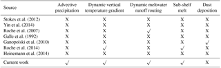
Stokes et al. (2012)Yin et al. (2014)Roche et al. (2007)Galle et al. (1992)Ganopolski et al. (2010)Roche et al. (2014)Heinemann et al. (2014)Table 1Feedbacks/interactions sporadically included in previous studies between the ice sheet model and the rest of the climate system, compared to the current study. None of these feedbacks/interactions include changes to land mask and bathymetry except for parameterized Bering Strait throughflow. Tick indicates included and cross indicates not included.
In this study, our objective is to develop a coupled ice sheet–climate model which encompasses most relevant feedbacks/interactions between the cryosphere and the atmosphere and ocean for continental glacial cycle scale contexts. Through a selection of ensemble parameters, we are also working towards bracketing the strength of these feedbacks across model ensembles. We also examined sensitivity to coupling time steps by setting up three similar simulations with different coupling time steps (100 years, 20 years, and 10 years). Features of note in the coupling and described in this paper include the following:
-
A dynamic vertical 2 m temperature gradient to improve the temperature downscaling from the atmosphere model to the ice sheet model.
-
An advective precipitation downscaling scheme which accounts for wind velocity and topographic slopes.
-
Dynamic meltwater routing.
-
An efficient scheme to extract approximate lat/long gridded ocean temperature fields from LOVECLIM ocean temperature profiles for sub-ice shelf melt computation.
Table 1 compares the interactions between ice sheets and climate models only infrequently included in previous coupled modelling studies to this study. There are two main interactions yet to be implemented. First, the dust cycle and its impact on atmospheric radiative balance and ice surface albedo (and therefore surface mass balance) awaits future work. Second, the LOVECLIM ocean component does not handle changing bathymetry and land mask over a transient run. It does have a parameterized Bering Strait throughflow which permits shutdown of throughflow when the local water depth approaches zero.
Climate models used for glacial cycle contexts need to be fast enough to simulate tens of thousands of years in a reasonable time interval, while also being complex enough to include all of the important climate dynamics. We tested every freely available fast model that included ocean, atmosphere, and dynamical sea ice components, and found a number of published models to be numerically unstable or otherwise unable to run or port. The only stable model with all these components was LOVECLIM. The other models tested and associated porting failures are as follows:
- SPEEDO –
-
compilation error using PGI and Intel compilers.
- FOAM (v. 1.5) –
-
no dynamic sea ice model; compilation error using PGI and Intel compilers.
- OSUVic (v. 2.8) –
-
compilation error.
- CSIRO-Mk3L (v. 1.2) –
-
compilation error using PGI, Intel, and GCC compilers; problem accessing fftw library.
This paper is structured as follows. We first introduce the models in Sect. 2. Next, we describe the coupling schemes between the ice sheet model and the atmosphere and the ocean models in Sect. 3. In this section, we use the last glacial inception time frame (120–110 ka) to show that the inclusion of each process coupling scheme can have significant impact on the evolution of major Northern Hemisphere (NH) ice sheets. In Sect. 4, we introduce our chosen set of ensemble parameters for the coupled model. In order to justify this choice of ensemble parameters, we examine the sensitivity of the coupled model to changes in each parameter for PD climate. We then sieve the ensemble parameter set using our coupled model with historical/PD initial and boundary conditions via a comparison against observational/reanalysis data.
2.1 LOVECLIM
LOVECLIM (version 1.3) is a coupled Earth systems model of intermediate complexity (EMIC), which consists of atmosphere (ECBilt), ocean with dynamic sea ice (CLIO) and vegetation (VECODE) modules. It is fast enough to simulate the last glacial inception (120 to 100 ka) in less than 3 weeks using a single computer core. Therefore, it has been used to simulate a wide range of different climates from the last glacial maximum (Roche et al., 2007) through the Holocene (Renssen et al., 2009) and the last millennium (Goosse et al., 2005) to the future (Goosse et al., 2007).
- Atmosphere
-
The atmospheric component (ECBilt, Opsteegh et al., 1998) is a spectral global quasi-geostrophic model, with T21 truncation, three vertical layers at 800, 500, and 200 hPa, and a time step of 4 h. The quasi-geostrophic structure of the model limits its ability to simulate equatorial variability and, hence, atmospheric interactions between the tropics and higher latitudes. To partially compensate for this, it has additional ageostrophic terms to improve the representation of Hadley cell dynamics (Opsteegh et al., 1998). Precipitation is computed from the precipitable water of the first layer according to a precipitation threshold for relative humidity (default 85%). The model contains simple schemes for short-wave and long-wave radiation, with radiative cloud cover prescribed by default (Haarsma et al., 1996).
- Ocean
-
The oceanic component (CLIO – Coupled Large-scale Ice Ocean) is a 3-D primitive equation model with Boussinesq and hydrostatic approximations. The model is discretized horizontally on a 3∘ × 3∘ Arakawa B-grid, with 20 vertical levels on a z coordinate. This coarse-resolution enables CLIO to run fast enough for glacial cycle simulations. A free surface and a parameterization of down-sloping currents (Campin and Goosse, 1999) enables CLIO to receive freshwater fluxes and capture some of their impacts on dense water flows off continental shelves. Goosse et al. (2001) describe the model in detail. A major limitation of this model (and challenge for many GCMs) for paleoclimate studies is that the bathymetry and land mask can not be changed during a transient run (specifically, there is no available nor described implementation that can do so).
- Sea ice
-
The sea ice component of CLIO is an updated version of the Fichefet and Maqueda (1997) dynamic–thermodynamic sea ice model. A visco-plastic rheology (Hibler, 1979) is used for horizontal stress balance. The thermodynamic component of the sea ice model considers sub-grid sea ice and snow cover thickness distribution, in addition to ice and snow sensible and latent heat storage.
- Vegetation
-
VECODE is a dynamic terrestrial vegetation model with a simplified terrestrial carbon cycle (Brovkin et al., 2002). The model simulates the dynamics of two plant functional types (trees and grasses), in addition to deserts, and evolves their grid-cell fractions. These fractions are determined by the contemporaneous climate state and terrestrial carbon pool. More details about the model can be found in Brovkin et al. (1997, 2002).
LOVECLIM has been tested for both interglacial and glacial contexts. Nikolova et al. (2013) found that the large-scale changes in climate simulated by LOVECLIM for the last interglacial were in approximate agreement with those indicated by available proxies (differences in the ±2.5 ∘C range for summer, and the −5 to 0 ∘C range for winter). These changes were also similar to that from a full complexity atmosphere–ocean general circulation model (CCSM3). However, due to stronger polar amplification in LOVECLIM, smaller sea ice extent and higher surface temperatures are simulated in LOVECLIM compared to CCSM3 for the interglacial.
During the Last Glacial Maximum, LOVECLIM overestimates both the minimum and maximum Southern Hemisphere sea ice cover compared to paleo-proxy data, while CCSM only overestimates the minimum sea ice extent (Roche et al., 2012). Roche et al. (2007) also found a reasonable agreement between the atmospheric and oceanic estimates of LOVECLIM and proxy data during the LGM (e.g., disappearance of much of the PD Siberian boreal forest, seasonal sea-ice extent, sea surface temperature). However, the Atlantic deep ocean circulation is stronger in their simulation, which opposes the general inference of weaker AMOC during the LGM.
2.2 GSM
The GSM is built around a thermo-mechanically coupled ice sheet model. It includes a 4 km deep permafrost-resolving bed thermal model (Tarasov and Peltier, 2007), fast surface drainage and lake solver (Tarasov and Peltier, 2006), visco-elastic bedrock deformation (Tarasov and Peltier, 1997), positive degree day surface mass balance with temperature dependent degree-day coefficients derived from energy balance modelling results (Tarasov and Peltier, 2002), sub-grid ice flow and surface mass balance for grid cells with incomplete ice cover (Morzadec and Tarasov, 2015), and various ice calving schemes for both marine and proglacial lake contexts (Tarasov et al., 2012). For the results herein, ice shelves are treated using a crude shallow ice approximation with fast sliding. The GSM is run at a 0.5∘ longitude by 0.25∘ latitude grid resolution.
The GSM has three new features that have not been previously documented. First, ice calving has been upgraded to the more physically based scheme from DeConto and Pollard (2016). However, our implementation imposes the additional condition that the ice cliff failure mechanism is only imposed at ice marginal grid cells. Second, a temperature-dependent sub-shelf melt scheme that also depends on adjacent subglacial meltwater discharge from the grounded ice sheet has been added. The melt is proportional to the water temperature to the power 1.6 and to proximal subglacial meltwater discharge following the Greenland fjord modelling results of Xu et al. (2013). We also impose a quadratic dependence on ice thickness to concentrate sub-shelf melt near deep grounding lines in accord with the results of process modelling (e.g., Jacobs et al., 1992). Finally, a first-order approximation to geoidal deflection is now included. Details of these schemes will be in an upcoming submission that fully describes the revised GSM.
2.3 Model initialization
For the results herein, PD and glacial inception model runs are initiated with PD ice sheet thickness. The initial bed-thermal temperature field is set to the PD resultant field from a mix of best-fit past calibrated and ongoing calibration model runs (i.e., without LOVECLIM as in Tarasov et al., 2012 for North America).
To initialize the temperature field of existing ice sheets, results from previous transient runs are usually used in the GSM. However, this does not work for a cold start from PD fields, as the PD ice thickness fields will not line up fully with model results. As such, the ice temperature field is initially linearly interpolated from surface temperature to a basal temperature of −3 ∘C. This enforces a frozen base to ensure a smooth spin-up and also provides warm enough ice to generate significant ice velocities. Ice velocity fields are then computed. The ice thermodynamics are subsequently partially spun-up over 5000 years (with fully coupled bed-thermal evolution). When the results of pre-Eemian Greenland and Antarctic calibrations become available, this will be used to initialize the respective Eemian ice sheet temperature and ice thickness fields.
Glacial inception surface topography is also offset from PD by the amount required to remove PD topographic discrepancies (to observed) from some past best fit calibration model runs.
As detailed below, the climate model is spun-up over an ensemble parameter dependent time interval prior to onset of the coupled model run.
The coupler is designed to regrid and exchange data between the ice sheet model (GSM) and LOVECLIM (ECBilt and CLIO) in both directions with minimal adjustment to the model code. Figure 1 displays all the fields the coupler transfers between different component models and the processes involved.
Due to the computational costs of coupling and trivial variations of ice sheets over small timescales, the ice model and the climate model run for a certain number of years before receiving updated fields from the other model. However, using large coupling time steps can also introduce errors into the results. To test the effect of the coupling time step on ice sheet evolution, we used three different coupling steps (100 years, 20 years, and 10 years) to simulate the last glacial inception starting at 120 ka. With identical boundary and initial conditions for all three simulations, runs with 10-year and 20-year coupling steps have less than a maximum of 3 % difference in ice volume (Fig. 2). However, the 100-year coupling-step run (red line in Fig. 2) strongly diverges from the other two during the retreat phase. This ice volume divergence is mostly due to a thinner ice in North America (NA) and Eurasia (EA), and a less southern extent of the NA ice sheet. A weaker response with longer coupling time steps is expected given the delay in updating climate and ice boundary conditions for the GSM and LOVECLIM, respectively. Given these results, we choose 20 years as the coupling step for all of our ensemble simulations (due in part to the not insignificant overhead with the coupler as currently coded/scripted).

Figure 1Components of the climate system and the interactions between them included in the coupled model. The section numbers denote the section of this paper in which each process is described in detail. Atmospheric fields passed from ECBilt to the GSM are monthly climatologies.
The ice sheet model exchanges data with both the atmosphere and the ocean models at the end of each coupling step. The fields that are passed are described in detail below.
3.1 Atmosphere to ice
At the end of each coupling time step, the coupler receives climate fields averaged over the last 10 years from ECBilt and converts them to monthly-mean values. These fields include the following:
-
2 m near surface air temperature and standard deviation;
-
vertical 2 m temperature gradient;
-
precipitation;
-
evaporation;
-
and latitudinal and longitudinal components of wind and the standard deviation of each.
LOVECLIM computes both 2 m near surface air temperatures (T2m) and surface (or skin) temperatures. We note at least one previous study has indicated the usage of LOVECLIM surface temperature for ice sheet modelling contexts (Roche et al., 2014), which we find problematic. Surface melt determination using positive degree days requires the T2m, and rain/snow fraction determination will be more accurately estimated with the T2m than the surface temperature. Ice thermodynamics would properly use the surface temperature, but this can be alleviated in part if the ice sheet model limits surface temperatures to 0 ∘C over ice and snow for the ice thermodynamics.
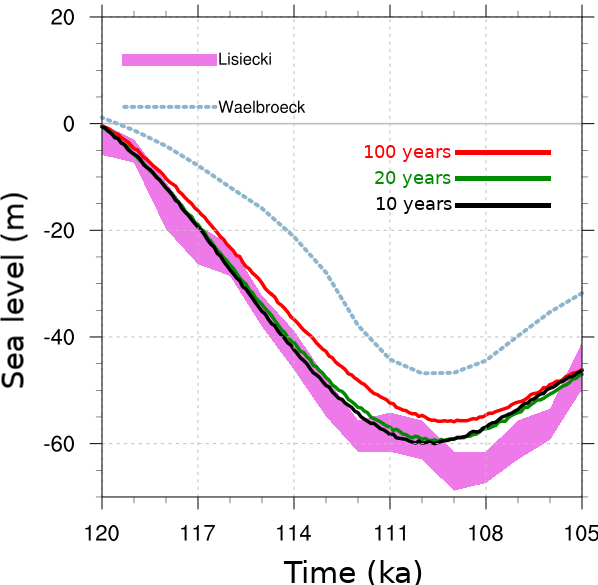
Figure 2Total ice volume in sea level equivalent (m) at last glacial inception, synchronously coupled with 100-year, 20-year, and 10-year time steps.
Given the simplified boundary layer physics of LOVECLIM, it may be that some weighted average of its T2m and surface temperature is a more appropriate estimate of “true” 2 m temperature. As shown in the Supplement, a raw average gives somewhat better overall fits to ERA40 2 m temperatures over Greenland and Antarctica but worse fits for July over North America and especially Eurasia using the default LOVECLIM tuning. Given these mixed results (and the possibility that after retuning the average of T2m and surface temperature would give better fits), we provide an option in the coupler to extract this average temperature from LOVECLIM instead of T2m.
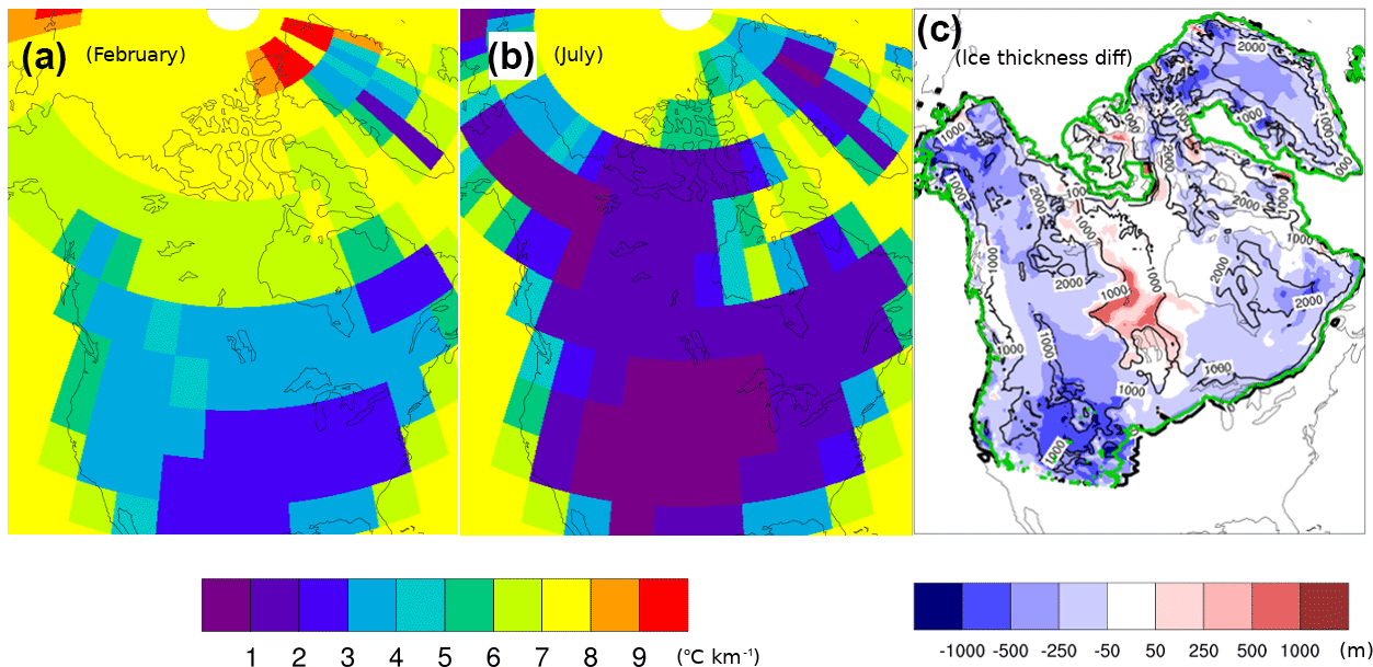
Figure 3Vertical temperature lapse rate calculated by the coupler at PD over NA in (a) February and (b) July. (c) Shows the ice thickness difference between dynamic and constant 6.5 K km−1 lapse rate (control) runs after running for 2 kyr, starting from the same 110 ka configuration. Black contours show the ice thickness in the control run. Thick black and green contours show the ice margin in the control and dynamic lapse rate run, respectively.
The large difference in spatial resolution of the two models necessitates horizontal and vertical downscaling of the climatic fields. The GSM receives climatic fields on the LOVECLIM grid, and downscales them to its own grid resolution using bilinear interpolation.
The downscaled standard deviation of temperature (using 4-hourly ECBilt data for each month averaged over the last 10 years of each coupling time step) is used to compute monthly positive degree days, with the usual assumption of a Gaussian distribution around the monthly mean. This is opposed to the traditional practice of assuming a constant value, usually between 5 and 7 ∘C.
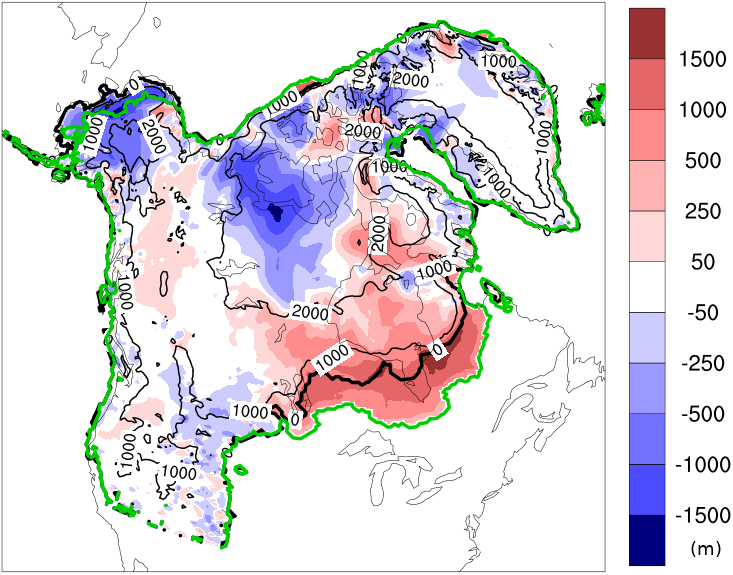
Figure 4Impact of advective precipitation downscaling inclusion in the coupled model; NA ice thickness difference at 110 ka between simulations with and without the advective precipitation method. Contours show the ice thickness in the control run. Thick black and green contours show the ice margin in the control and advective precipitation run, respectively. LOVECLIM parameters are set to default values.
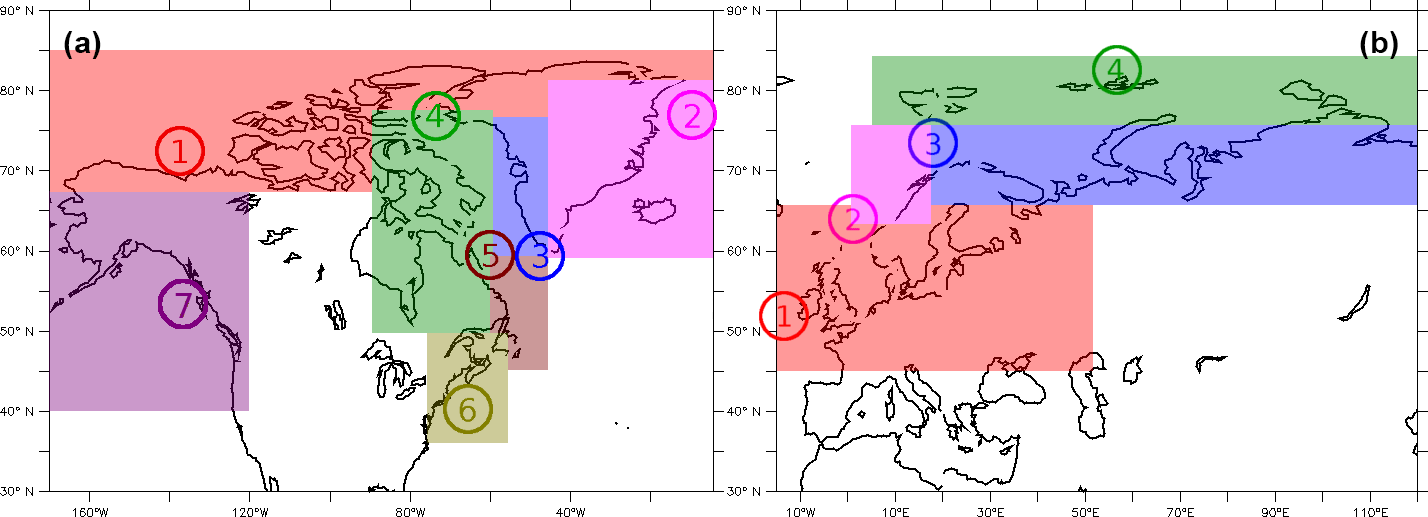
Figure 5The upstream ocean temperature profile sites and corresponding downstream sectors assigned to these profiles for ocean–ice coupling in (a) NA and Greenland and (b) EA.
3.1.1 Vertical temperature gradient
Large grid resolution differences between ECBilt and the GSM result in surface elevation differences between the two models, especially in places with steep topography. The altitude dependence of temperature in such regions can drastically affect the type of precipitation and surface mass balance of the ice sheet. Therefore, in addition to horizontally downscaling the temperature from LOVECLIM to the GSM, a vertical correction of temperature is required.
By monitoring 25 sites spread over a 15 650 km2 area and with an altitude range from 130 to 2010 m on the Prince of Wales Icefield for 2 years, Marshall et al. (2007) found a mean daily vertical surface temperature gradient of −4.1 K km−1, with an average summer gradient of −4.3 K km−1. These values are less than the standard mean free-air temperature lapse rate that is often used for extrapolations of sea level temperature to higher altitudes (−6.5 K km−1) (e.g., Glover, 1999; Arnold et al., 2006; Raper and Braithwaite, 2006). Marshall et al. (2007) also find a vertical surface temperature gradient of −6 to −7 K km−1 on steep regions in summer, and around −2 K km−1 in regions where northerly anticyclonic flow is more common. In addition, Gardner et al. (2009) find significant spatio-temporal variations in vertical temperature gradients across four glaciers in the Canadian High Arctic.
The GSM uses the near-surface vertical T2m gradient calculated by the coupler at the end of each time step to downscale the temperature field over its high-resolution grid. In each LOVECLIM grid cell, the coupler first determines the highest and lowest elevations from the GSM topography constrained by the cell's boundary. Next, the T2m for these two elevations is calculated using the inherited scheme from the LOVECLIM atmospheric model (as detailed in Roche et al., 2014). The resulting temperature and elevation difference between the two points is then used to calculate the temperature lapse rate in that LOVECLIM grid cell.
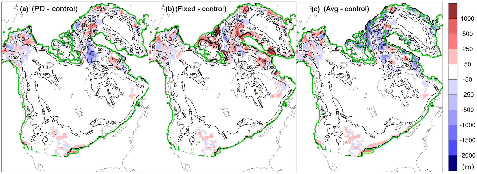
Figure 6Ice thickness difference from the control run (dynamic ocean temperature) at 108 ka for three test runs starting from the same 110 ka control run restart. The three test runs are as follows: (a) PD ocean temperature run, (b) the fixed ocean temperature at −2 ∘C run, and (c) the temperature averaged over ocean layers run. Contours show the ice thickness in the control run. Thick black and green contours show the ice margin in the control and the other run in each of the panels, respectively.
Figure 3a and b show the present-day vertical T2m lapse rate calculated by the coupler for summer and winter. The derived lapse rate has strong spatial and temporal variation over NA and Greenland. The impact of this variation is shown in Fig. 3c. Starting from the same 110 ka configuration, the difference in ice thickness after 2 kyr between a dynamic temperature lapse rate run and a control run (default LOVECLIM parameters) with a 6.5 K km−1 lapse rate can reach over 1 km.
Evaluating the appropriateness of our vertical temperature downscaling approach is difficult, especially when considering glacial/interglacial changes. Using a global climate model (CCSM3), Erokhina et al. (2017) found significantly larger surface slope lapse rate values over the Greenland ice sheet during the LGM compared to pre-industrial values (February mean increase of about 3.7 K km−1 and about 0.9 K km−1 for July). In contrast, our T2m mean LGM lapse rate over Greenland is 0.8 K km−1 stronger for February and 0.2 K km−1 weaker for July compared to that of the PD. However, neither lapse rate is an accurate a priori choice for vertical downscaling. A need remains for a multi-resolution modelling study to compare a “true” downscaling vertical temperature gradient with the various possible lapse rates that can be derived from a single resolution model.
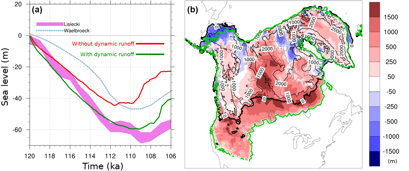
Figure 7The impact of meltwater runoff inclusion in the coupled model; (a) total ice volume evolution at glacial inception with (green) and without (red) dynamic meltwater routing, and (b) NA ice thickness difference at 110 ka with and without dynamic runoff routing. Contours show the ice thickness in the simulation without dynamic runoff routing. Thick black and green contours show the ice margin in the control and dynamic runoff routing run, respectively.
3.1.2 Advective precipitation downscaling
LOVECLIM calculates evaporation, rain, and snow for each grid cell based on its coarse-resolution surface topography and temperature fields. These fields require downscaling to the higher resolution GSM grid. A common approach is to linearly interpolate both precipitation and evaporation fields onto the high-resolution ice sheet model grid, calculate the net precipitation amount, and finally determine the amount of rain and snow for each grid cell using the downscaled temperature. However, linear interpolation does not correct the damped orographic forcing due to a coarse-resolution climate model grid. Here, we apply a new approach to precipitation downscaling that also accounts for orographic forcing at the ice sheet grid resolution.
The scheme assumes that orographic precipitation effects for upslope winds will be proportional to the vertical velocity induced by the surface slope and, therefore, to the dot product of the horizontal wind velocity and surface slope (SGSM and SATM) with the latter given by
The k in the above equations indexes a representative range of wind vectors for each month. To simplify the coupling and still capture wind variation, we use monthly climatologies of mean wind velocity and its standard deviation in the determination of SGSM and SATM. We compute the advective precipitation correction factor (fkp) using the S's as a function of mean and mean ± one standard deviation. We then sum over these factors with appropriate weights (W(k)) for a Gaussian distribution. This correction is based either on the ratio of the S terms for SATM>0 (i.e., upslope winds) or on their difference (to transition into precipitation shadowing). In detail, with the inclusion of a regularization term (μ, that governs the transition to precipitation shadowing) and bounds (fpmin and fpmax), this takes the following form:
The loop is carried out for each point on the GSM grid. The net correction for each corresponding point on the lower resolution atmospheric grid is then accumulated to generate a rescaling coefficient that is mapped back to each on the GSM grid to ensure mass conservation. The scheme is currently implemented with μ=0.005 and fpmin=0.2 and fpmax=5.0.
The new advective precipitation downscaling results in increased ice sheet volume and southern extent for the North American ice sheet during the inception phase. This increase is largest for the southeastern sector of the ice sheet (Fig. 4). Ice thickness also decreases in some regions due to precipitation shadowing.
3.1.3 No bias correction
Studies from Goosse et al. (2007), Mairesse et al. (2013), Renssen et al. (2009), Widmann et al. (2010), Roche et al. (2007), van Meerbeeck et al. (2009), and Otto-Bliesner and Brady (2010) demonstrate LOVECLIM's overall ability to simulate the last millennium, the Holocene, and the Last Glacial Maximum (LGM) climates in agreement with observed and proxy records. However, the model still suffers from a high temperature bias at low latitudes, an overly symmetric distribution of precipitation between the two hemispheres, an overestimation of precipitation and vegetation cover in the subtropics, weak atmospheric circulation, and an overestimation of the ocean heat uptake over the last decades (Goosse et al., 2010).
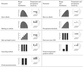
Table 2Ensemble parameters that are varied in the historical transient simulation ensemble. Column 2: the distribution of parameter values versus their range for each parameter. Column 3: change in 1950–1980 CE mean summer 2 m temperature and winter precipitation over four selected regions when each parameter is varied independently from its minimum to its maximum value. In each sensitivity run, all the other parameters are fixed to LOVECLIM default values, with a spin-up length of 4000 years, simple upscaling method, default LOVECLIM cloud radiative forcing, a start year of 1500 CE, and a dynamic vertical temperature lapse rate.
The extent to which these biases are due to the tuning of LOVECLIM parameters and missing couplings with the rest of the Earth/climate system is unclear. Therefore, we do not apply a bias correction to atmospheric fields and instead examine the extent to which an ensemble parameter sweep can reduce the bias. As detailed below, a reduction in the PD regional temperature and precipitation bias occurs for various members of our perturbed parameter ensemble.
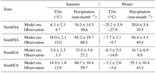
The control run (with all LOVECLIM parameters set to their default values, and other coupling parameters as described in the caption of Table 2) shows the highest temperature bias in the “South NA” region (∼5 ∘C), with slightly colder temperatures in the “North NA” (∼1 ∘C). The temperature bias over EA is less significant, and is also less latitude dependent (both “North EA” and “South EA” are biased by <2 ∘C). A reduction in the regional temperature and precipitation bias is observed in various members of our ensemble of simulations for the PD, as introduced below. The regional temperature and precipitation bias relative to observed (Table 3) over NA and EA can reach zero for some ensemble members for both summer and winter. Although there is no individual run with zero bias in all the regions, a number of selected runs show reduced temperature biases (between −1 and 1 ∘C) in all four regions compared to that of the control run.
Table 3The sieved sub-ensemble and observed mean summer and winter 2 m temperature and precipitation averaged over four latitudinal bands for the 1950–1980 CE interval.
3.2 Ocean to ice: sub-shelf melt
Sub-ice shelf melt is a challenge for paleo coupled ice sheet climate modelling given the dependence on unresolved basin-scale circulation. As a first-order approximation, we assume that upstream ocean temperature at the same depth corresponds to the local sub-shelf temperature. To facilitate fast and simplified coupling, given the complexity of ocean grids in most ocean general circulation models, we only extract upstream ocean temperature vertical profiles from LOVECLIM at the end of each coupling time step for a number of chosen index sites as indicated in Fig. 5 and use these for downstream marine sectors. We selected these sites (seven over NA + Greenland and four over EA) by examining the PD ocean temperature climatologies from CLIO (at various depths) while taking ocean currents into account. Our site selection was predicated on the constant bathymetry and land mask of CLIO and would need updating for a model with dynamic land mask/bathymetry. The downstream masks for the profile sites extend onto land where applicable when grounding line retreat beyond the fixed ocean mask of CLIO (i.e., onto the land mask) is possible.
To test the impact of this regional disaggregation of ocean temperatures, we generated three test cases: ocean temperature forcing set to PD value, to −2 ∘C, and to the contemporaneous average across the above index sites. Starting from a 110 ka restart, all three options have local ice thickness differences greater than 1 km after 2 kyr compared to that with the standard coupling (Fig. 6).
3.3 Ice to atmosphere
Changes in both the topography and the ice mask can affect the global circulation patterns by influencing the stationary waves and the jet stream. At the end of each coupling time step, the coupler receives the updated topography and ice thickness fields from the GSM. The topography field is upscaled to the ECBilt grid and then used for the next LOVECLIM run step. Given the large difference in grid resolution, the choice of upscaling scheme is not clear a priori. Therefore, we have implemented three different schemes to upscale the topography from the GSM high-resolution grid to the ECBilt low-resolution grid.
3.3.1 Topography upscaling and ice mask
- The simple average method
-
In this method, the coupler simply calculates a weight for each high-resolution grid cell based on the fraction of the cell located inside the coarse grid cell. These weights are then used to calculate the average altitude of each ECBilt cell from the GSM orography.
- The envelope method
-
In the envelope method, a weighted standard deviation of the altitude of all the GSM cells inside the ECBilt cell is added to the simple average altitude from the previous method. The envelope method works reasonably well to preserve the overall topographic peaks, but it can introduce a phase shift in the terrain field, broaden ridges, and raise the height of even relatively broad valleys:
Here, Hi,j is the model terrain height, ω is a predefined weighting factor (in our experiments 0.5), and σi,j is the standard deviation at the model grid point.
- The silhouette method
-
The silhouette method combines the simple average altitude with a silhouette height. The silhouette height is defined as follows:
where Hmax is the maximum height of all GSM grid cells inside the ECBilt cell, Hsx and Hsy are the average peak heights obtained in each row and column of nested cells, and ω1 is the predefined weight. The silhouette height is then used to calculate the ECBilt cell altitude using:
Different combinations of the weighting factors ω1 and ω2 will draw the gridded terrain analysis toward preserving the peaks (ω2=1) or preserving the mean topographic height (ω2=0), which allows a greater degree of freedom to determine the model terrain analysis.
3.3.2 Ice mask
Another important consideration in the ice sheet–atmospheric coupling is the variation in ice extent, which changes the albedo calculated by ECBilt; this affects the temperature field over the region and globally. We used the ice thickness field generated by the GSM to create the ice mask needed by ECBilt. To do so, the high-resolution ice thickness field is first regridded to the ECBilt coarse-resolution grid using one of the methods mentioned above. Any cell in the resulting grid with more than 30 % ice coverage is then assumed to be ice covered.
Our choice of a 30 % threshold (as opposed to say 50 %) was motivated by the following logic. For any atmospheric grid cell covering an ice margin segment, the temperature passed to the GSM should most importantly reflect ice covered boundary conditions local to the ablations zone of the ice sheet. Allowance for subgrid advection of warmer air masses from adjacent ice-free land somewhat tempers this logic. Given potentially significant impacts on critical ablation temperatures and therefore ice sheet mass balance, this ice-fraction threshold deserves a sensitivity analysis (in future work).
3.4 Ice to ocean
3.4.1 Topographically self-consistent and mass conserving freshwater discharge
The melting of continental ice sheets provides a freshwater source to the ocean that affects global sea level and the AMOC. Dynamical ocean models indicate that the strength of the AMOC in the North Atlantic is sensitive to the freshwater budget at the sites of the formation of North Atlantic Deep Water (Rahmstorf, 1995).

Figure 8Selected north and south zones over North America and Eurasia for PD sensitivity analysis.
As the GSM self-consistently computes surface drainage (while conserving mass) for the evolving topography while LOVECLIM surface drainage is hard-coded for PD topography, precipitation within LOVECLIM is masked out where covered by the GSM grid. The coupler then distributes GSM freshwater ocean discharge to corresponding LOVECLIM ocean discharge grid cells. In areas where the GSM grid edge is terrestrial, the GSM discharge is added to the corresponding LOVECLIM grid cell for internal runoff routing. As topographic gradient changes from glacial isostatic adjustment (GIA) are small outside of the GSM grid, this scheme should give results close to what would be achieved with a drainage solver using a topography globally subject to GIA.
We describe the runoff routing in the coupler and the connection between the GSM and LOVECLIM drainage basins in more detail in the Supplement.
Figure 7a provides an example of how the inclusion of meltwater runoff in the coupled model improves ice sheet growth at glacial inception. Although the impact is small at the first stages of ice formation due to small ice volumes with negligible runoff rate changes, ice in the simulation including runoff grows faster as it gains more volume. The difference reaches its maximum at 110 ka, with about 50 % more ice in the run with dynamic drainage routing, including much thicker and more extensive ice over North America (Fig. 7b). Compared to the control run (no dynamic drainage routing), the AMOC strength drops by 15 %, and the sea ice extent shows an increase of 5 % in winter and ∼15 % in summer (not shown). The combination of these AMOC and sea ice changes yields a cooler summer in the run with dynamic drainage routing, which results in less ice sheet melt.
3.4.2 Bering Strait
The Bering Strait is a narrow strait with a present depth of approximately 50 m between Siberia and Alaska, through which relatively fresh North Pacific water is transported to the Arctic. From there, the North Pacific water is transported to the Greenland Sea and the North Atlantic. This less-saline water affects the upper ocean stratification and thus the strength of deep ocean convection and the AMOC, which in turn, has impacts on the global climate (Shaffer and Bendtsen, 1994; De Boer and Nof, 2004; Hu et al., 2008).
Due to the ice sheet growth and associated sea level lowering, the Bering Strait was often closed during glacial cycles, limiting the freshwater flow from the Pacific Ocean to the Arctic. LOVECLIM does not explicitly compute the direct connection between the Pacific and the Arctic through the Bering Strait, so the transport is parameterized by a linear function of the cross-strait sea level difference in accordance with geostrophic control theory (Goosse et al., 1997). The coupler interpolates the Bering Strait scaling at each coupling step between the PD value (0.3, 50 m depth) and a closed strait (0.0, 0 m depth) using the relative sea level at the Bering Strait as computed by the GSM. Given the shallowness of the strait, the accuracy of the GSM in representing sea level changes (based on its viscoelastic bedrock response and first-order Geoidal correction) plays a potentially important role here.
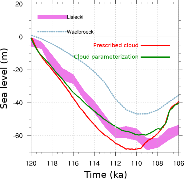
Figure 9Total ice volume at the last glacial inception with the cloud parameterization (green) and the PD cloud cover forcing (red).
Ensemble parameters were initially chosen by judgement of their control of a physical aspect of ice sheet–climate interaction (e.g., albedo) or by their potential impact on the coupling between the ice sheet and the climate (e.g., upscaling method) (Table 2). This choice was then validated by the following sensitivity analysis.
As the context of the model development is glacial inception and deglaciation, we are interested in the ensemble performance for climate metrics which control the growth and decay of the NH ice sheets during these two stages. Therefore, we use summer 2 m temperature and winter precipitation over land. To enable comparison against observations, our sensitivity analysis is based on transient runs over the historical interval (up to 1980 CE).
Since glacial inception and deglaciation are triggered at different latitudes in NA and EA, we have divided each continent into diagnostic north and south zones (called “NorthNA”, “SouthNA”, “NorthEA”, and “SouthEA”). The sensitivity of the coupled model is tracked for each individual zone. The “NorthNA” and “SouthNA” zones cover latitude ranges of 65–75 and 40–60∘ N over NA, respectively. “NorthEA” and “SouthEA” are defined over 70–80 and 55–70∘ N latitude bands, respectively. The regional boundaries are illustrated in Fig. 8.
The third column in Table 2 shows the sensitivity of T2m and precipitation in the coupled model to changes in each parameter through its range for four different latitudinal bands over NA and EA averaged over the 1950–1980 interval. For easier comparison, all figures use the same temperature and precipitation scales. The sensitivity to each parameter for the four regions is different for temperature and precipitation. For instance, switching between PD radiative cloud forcing and cloud parameterization strongly affects both temperature and precipitation over all regions, while changing the snow albedo has its strongest impact on EA temperatures and precipitation (Table 2). Each of the ensemble parameters has an impact of at least 4 ∘C on temperature and/or 1 cm month−1 on precipitation over the given parameter ranges. We take this as justification for their continued use as ensemble parameters.
In the following subsections, we further describe the parameters used in the ensemble simulation. Later, we will show that the chosen set of ensemble parameters is adequate for bracketing the relevant (temperature and precipitation) fields of the climate system.
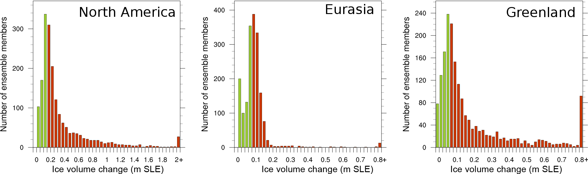
Figure 10The distribution of ice volume change over NA, EA, and Greenland, between 1700 and 1980 CE in 2000 ensemble runs. Green bars represent the selected 500 ensemble members, and red bars represent the rest. SLE stands for sea level equivalent.
4.1 Snow and ice albedo
Changes in the snow and ice area and type have an amplifying effect on climate by modifying the surface albedo. During summer, the balance between absorbed and reflected solar energy at the ice sheet surface is the dominant factor controlling surface melt variability in the ablation zone (van den Broeke et al., 2008). The parameterization of the surface albedo in LOVECLIM takes the state of the surface (frozen or melting) and the thickness of the snow and ice covers into account (Goosse et al., 2010). We include all types of snow and ice albedo (i.e., snow, melting snow, and bare ice) in our ensemble parameter set.
The snow albedo, bare ice albedo, and melting ice albedo rows in Table 2 show the range of albedo values for each type and their climate sensitivity. Increasing snow albedo results in a reduction of winter precipitation over all four regions with an extended effect over summer temperatures, as expected. However, the same feedback is not as straightforward for bare ice albedo and melting ice albedo. Although the increase in bare ice albedo shows an expected cooling effect over all regions with a smaller influence on precipitation, an increase in melting ice albedo causes all regions to get between 4 and 6 ∘C warmer and increases the winter precipitation.
4.2 Climate initialization/spin-up
Before starting a coupled transient climate simulation, it is necessary to allow the atmosphere and ocean to adjust to the initial boundary conditions and external forcings. Model spin-up, and therefore the initial state of the climate system, can be a major source of uncertainty in climate modelling especially given the millennial timescale of deep ocean circulation.
The general approach to spin-up the ocean is to run the ocean to an equilibrium state under fixed external forcings (e.g., Manabe et al., 1991; Johns et al., 1997). However, as the climate system is unlikely to ever be in equilibrium, this choice lacks justification. We include two parameters to control the initial state of the system: LOVECLIM spin-up start year, and LOVECLIM spin-up length. All spin-ups are performed using transient orbital and CO2 forcings ranging from 3000 to 5000 years but without the GSM coupling. The combination of these two spin-up control parameters results in slightly different coupled transient start times, each with different initial ocean and atmosphere states. For the runs herein, we constrain the spin-up to end between 1400 and 1600 CE. Increasing the spin-up length has a cooling and drying effect in the coupled model with PD boundary and initial conditions, while starting the transient coupled run from earlier years results in slightly warmer and wetter conditions (Table 2).
4.3 Upscaling
The three different upscaling methods described in Sect. 3.3.1 are evenly distributed between ensemble members as shown in Table 2. By switching between three methods, we calculate the highest temperature and precipitation changes over four regions and plot them in the last column of Table 2. The highest temperature sensitivity to the upscaling method is recorded in NorthNA followed by the NorthEA zones, and the highest precipitation sensitivity is seen in the SouthEA zone.
4.4 Precipitation threshold
ECBilt only accounts for humidity, and thus precipitable water, between the surface and the 500 hPa layer. Above 500 hPa, the atmosphere is assumed to be dry, meaning that all the water transported by atmospheric flows into this region precipitates. Below the 500 hPa layer, ECBilt precipitates all the excess water above a fixed threshold (default 0.83) multiplied by the vertically integrated saturation specific humidity (Goosse et al., 2010). This parameter has the largest relative impact for NorthEA temperature (4 ∘C over the parameter range equivalent to 60 % of mean).
4.5 Cloud radiation parameterization
The representation of clouds is one of the largest sources of uncertainty in models. They play an important role in regulating the surface energy balance of ice sheets, with competing warming and cooling effects at the surface through changes to short-wave and long-wave radiative fluxes. The effect of ice sheets on cloud formation is also significant. The growth of ice sheets results in tropospheric cooling and a reduction in humidity. This colder and drier troposphere displaces the upper tropospheric stratiform clouds downward, and reduces the low level stratiform cloud cover around the ice sheets (Hewitt and Mitchell, 1997).
The total downward and upward long-wave radiative scheme in ECBilt is a function of the vertical profile of the temperature, the concentration of various GHGs, and the humidity, and is computed for both clear sky and cloudy conditions. The radiation computed for each grid cell is then the weighted average of these two conditions based on the cloud coverage. The default ECBilt configuration prescribes radiative cloud coverage to the PD ISCCP D2 dataset (Rossow, 1996). The total downward and upward short-wave radiative fluxes depend on the transmissivity of the atmosphere, which also relies on the prescribed cloud cover (Goosse et al., 2010).
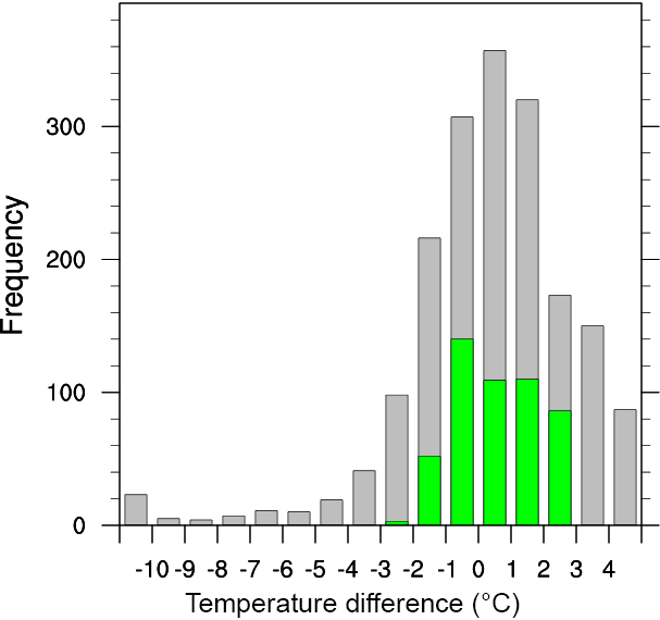
Figure 12The distribution of global annual mean 2 m temperature difference between ensemble members and observations averaged from 1950 to 1980 CE. Grey and green bars represent the 2000 ensemble members and the top-performing 500 ensemble members, respectively.
Given the importance of cloud radiative feedbacks on ice sheet evolution, the use of a prescribed PD cloud cover for paleoclimate modelling lacks justification. Therefore, we have added a simple cloud parameterization scheme similar to the precipitation parameterization scheme described in Sect. 4.4. The only difference here is the humidity threshold for cloud formation, which is assumed to be 10 % less than the precipitation threshold, allowing cloud cover without precipitation. Including the dynamic cloud cover radiation feedback in the coupled model slightly decreases the total ice volume at glacial inception (Fig. 9) through reduced humidity during glacial conditions reducing the cloud cover.
As evident in the “Temperature and precipitation sensitivity” column in Table 2, regional temperature and precipitation are sensitive to each of our ensemble parameters in the coupled model. However, due to the non-linearity of the climate system, the combined effect can be significantly different. In the next section, we explore the coupled model response to all these parameters in an ensemble of simulations.
The fast runtime of the coupled model permitted an initial ensemble of 2000 PD simulations using the fully coupled GSM-LOVECLIM and varying the model parameters described above. We chose the PD interval to permit a comparison of the coupled model output against observational data and to select a better fit sub-ensemble for transient glacial inception runs. All simulations are spun-up using transient forcings (orbital, Berger, 1978; Law Dome for recent CO2, Etheridge et al., 1998; and Dome C for pre-industrial to 5 ka CO2, Monnin et al., 2001) for 3000 to 5000 years without the GSM coupled, followed by a transient coupled run ending at year 1980. The ensemble parameter values were generated via a Latin hypercube scheme with increased weighting near LOVECLIM default values.
Given a priority to “bracket reality” and limitations of the component models, we chose to not use climate characteristics for the sub-ensemble filter. Our focus on coupled ice and climate and our choice to avoid bias corrections led to a trial criteria based on ice volume changes (between 1700 and 1980 CE). Therefore, we used the PD simulated NH ice sheet growth to sieve out parameter vectors with major surface mass balance biases. We first considered a less than 0.1 m SLE change in the ice volume requirement for each of the three northern ice sheet regions. However, this already fell below our target size of 500 simulations with NA being the problematic region (Fig. 10). Therefore, we changed the criterion to be the 500 runs with the least amount of ice volume change over each ice sheet. The sub-ensemble NA simulations have an ice volume less than 0.15 m SLE (sea level equivalent) and ice volume changes for the other two ice sheets are well below 0.1 m SLE (Fig. 10). Crucial to our “reality bracketing”, there are about 80 sub-ensemble members with ice loss over the given time interval.
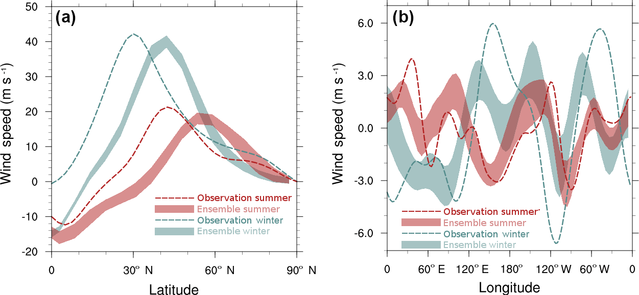
Figure 13(a) The zonal average of the zonal component of the 200 hPa wind velocity, and (b) the meridional average of the meridional component of the 200 hPa wind velocity over the NH. Filled areas show the model ensemble mean and the two standard deviation range. Dashed lines represent observational data. Blue is for winter, and red is for summer.
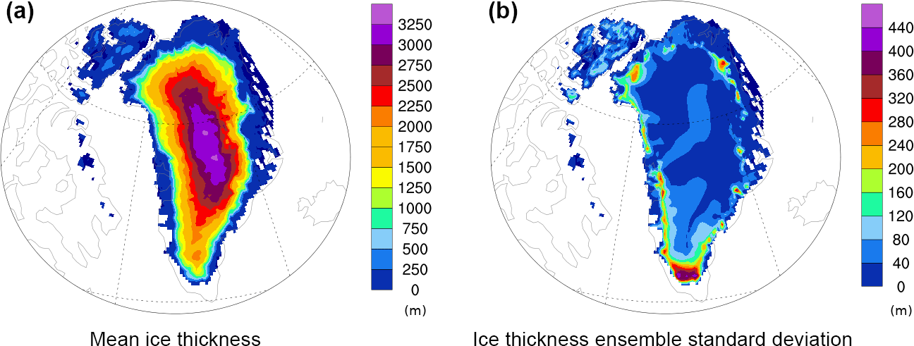
From here on, we focus on the 500 member sub-ensemble results. Figure 11 shows the Greenland region ensemble mean thickness and standard deviation at PD. The largest ice thickness changes occur at the southern margins of the Greenland ice sheet. Eastern NA ice expansion is concentrated in the high Arctic (Ellesmere Island and adjacent) where PD ice caps exist.
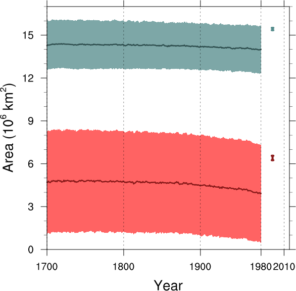
Figure 14Maximum (March – blue) and minimum (September – red) sea ice area ensemble mean ± one standard deviation. The vertical lines represent observational 1981–2010 March and September mean sea ice area within one standard deviation (Walsh et al., 2015).
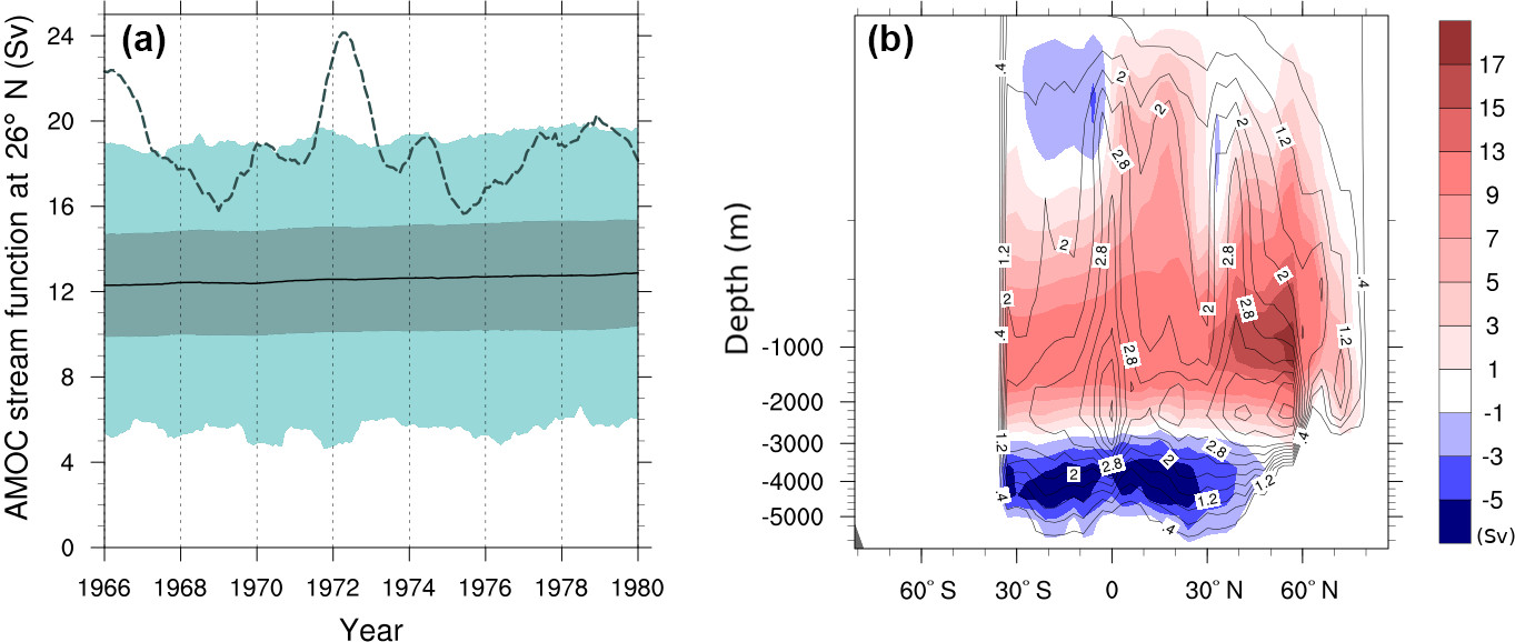
Figure 15(a) Maximum AMOC strength at 26∘ N between 1966 and 1980 CE. The black solid line represents the ensemble mean; the dark blue area represents the ensemble mean ± one standard deviation; the light blue area is bounded by the simulations with the maximum and minimum AMOC strength (time averaged); and the dashed line represents ORA-S3 (Balmaseda et al., 2008). (b), AMOC stream-function mean (filled colours) and ensemble standard deviation (contour lines).
5.1 The 2 m temperature and precipitation
The ensemble distribution of the annual mean global T2m anomaly with respect to observations shows that the majority of the ensemble members fall within ±3 ∘C of observations (grey bars in Fig. 12). However, as ice sheet build up is a function of both temperature and precipitation, most of the warm biased simulations fail to maintain ice-free conditions over NA and EA during PD due to a high winter precipitation bias (Table 3).
Our four latitudinal bands defined in Sect. 4 (Table 3) provide more relevant temperature metrics for NH ice sheet contexts. All four regions have higher ensemble mean seasonal T2m and precipitation compared to observations. However, the observations are covered well within two standard deviations for all regions, and temperature is covered within one standard deviation for most regions.
The seasonal cycle provides a partial test of a model's response to orbital forcing on Milankovitch scales. The ensemble mean seasonal cycle (difference between mean summer and mean winter) is within one standard deviation of the reanalysis data for all regions and for both temperature and precipitation (Table 3). Furthermore, aside from NorthEA, the diagnostic regions have a mean difference between summer and winter ensemble temperatures within a degree Celsius of that of the reanalysis climatology.
5.2 Northern Hemisphere jet stream
Jet stream latitude and oscillations have a strong control over storm tracks and the boundary between polar and subtropical air masses. Therefore, they are critical factors in controlling where and when an ice sheet margin advances or retreats. Due to the low vertical resolution of ECBilt, we compare the ensemble zonal mean of the 200 hPa zonal wind (as opposed to the more usual 300 hPa diagnostic level) with observations in winter and summer over NA and EA (Fig. 13a). The ensemble shows good agreement in capturing the maximum zonal velocity, but there is a 10 to 15∘ shift northward in the latitude of the jet in both seasons. This is likely due to the reduced temperature gradient between low and high latitude.
We also compare the 30–80∘ N meridionally averaged meridional wind at 200 hPa of the ensemble mean and the observations to diagnose the Rossby waves. In the summer, the longitudes of the troughs and ridges from the Pacific Ocean to the Atlantic Ocean largely match the reanalysis output within ensemble range (red line in Fig. 13b) with the largest discrepancies over the Eurasian region. During the winter, although the general pattern of the jet stream oscillations still agrees between the model and the observations (troughs over Eurasia and North America), the mismatch between ensemble members and observations becomes more significant given the higher Rossby wave number of the model ensemble.
5.3 Sea ice
High latitude sea ice acts as an insulator for both heat and moisture between the atmosphere and ocean, which are the two controlling factors for terrestrial ice sheet surface mass balance. We use the area and minimum latitude extent of the NH sea ice as relevant diagnostics. The general warm bias of the ensemble is reflected in the reduced ice area of the ensemble for both seasons, barely capturing the observed area within the one standard deviation range of the ensemble (Fig. 14). Both March (maximum) and September (minimum) NH sea ice areas show gradual decreases in the ensemble mean as the greenhouse gas concentration increases in the model.
Our filter condition for our sub-ensemble still permits a wide response of modelled components. For instance, averaging from 1950 to 1980 CE, the Pacific Ocean sea ice shows higher sensitivity to ensemble parameters during its maximum seasonal extent than the Atlantic. The sea ice minimum latitude in the Pacific ranges from 60 to 45∘ N (not shown), in comparison to the observed value of 60∘ N (Walsh et al., 2015).
5.4 AMOC
The AMOC transports large amounts of heat and salinity between high and low latitudes. Both paleoclimate proxy records (McManus et al., 2004) and climate model simulations (Liu et al., 2009) show that the AMOC experiences significant changes over a glacial cycle.
Our “bounding reality” criteria is not met for at least two AMOC features of the sub-ensemble. The PD ensemble mean AMOC strength is weaker than the reanalysis data from European Centre of Medium-Range Weather Forecasts (ECMWF ORA-S3, Balmaseda et al., 2008). The temporal mean of the reanalysis data is only captured by the maximum ensemble range (Fig. 15a). The ensemble mean shows a slight increase in the AMOC strength from 1965 to 1980 CE, which is not seen in ORA-S3. Furthermore, the temporal variability of the CLIO AMOC lacks the strong amplitude of the low frequency component of observations (as displayed by the maximum and minimum – time averaged – AMOC strength runs in Fig. 15a).
The maximum AMOC stream function strength is seen around 50∘ N at 1 km depth. The ensemble variance is also highest in the same region, in addition to 0∘ latitude at the same depth (Fig. 15b).
We have coupled an Earth system model of intermediate complexity (LOVECLIM) with a 3-D thermomechanical coupled ice sheet systems model (GSM) using LCice 1.0. The coupling efficiently captures most of the relevant feedbacks/interactions between the ice sheet and the atmosphere and ocean models. Our coupled model includes a parameterized sub-shelf melt using upstream ocean vertical temperature profiles, a simple cloud parameterization scheme to improve the radiative forcing representation in the atmosphere model, a dynamical vertical temperature gradient, and a dynamic meltwater runoff routing. We also introduce a new precipitation downscaling scheme that accounts for the change in surface slopes between the coarse-resolution climate model grid and the higher resolution ice sheet model grid. Each of the above features has significant impact on modelled ice thickness (shown directly or via changes in temperature and/or precipitation).
We have presented a set of ensemble parameters to generate an ensemble of runs that “bracket reality” and have shown that each ensemble parameter has a significant impact on modelled PD regional temperatures and/or precipitation. The new coupled model was subject to a Latin hypercube parameter sweep of 2000 ensemble simulations for PD boundary and initial conditions. We extracted a sub-ensemble of 500 model runs according to modelled PD NH ice volume changes. The mean of the sub-ensemble is warm- and wet-biased for the NH ice sheet region. However, the model ensemble still brackets reanalysis precipitation and temperature fields within two (ensemble) standard deviations for all regions and within one standard deviation for half of the regions for the case of temperature.
The ensemble's performance at capturing the seasonal cycle is much better. The ensemble mean difference between summer and winter for all four regions is well within one standard deviation of reanalysis values for both temperature and precipitation (and within one degree Celsius for three of the four regions). This provides some confidence that the model responds adequately to orbital forcing (at least for components that operate on sub-annual timescales).
The “reality bracketing” criterion is not met for certain features of atmospheric circulation (especially the wintertime Rossby wave number) and AMOC strength and variance. Another key limitation of LOVECLIM is the inability to change bathymetry and land mask (aside from the parameterized Bering Strait throughflow). The paleoclimate and ice sheet modelling communities would be well served by a modern successor to LOVECLIM for large ensemble glacial cycle timescale contexts that permitted transient changes to bathymetry and land mask.
The coupled model runs at about 1 kyr day−1 on one core; therefore, it enables large ensembles of full glacial cycle integrations. As a step towards this, our subset of 500 ensemble members is being used for inception and deglaciation ensemble experiments with the coupled model.
LOVECLIM is freely available from http://www.climate.be/modx/index.php?id=81 (Goosse et al., 2010). The GSM will be made publicly available in 1–2 years (as detailed code documentation and further upgrades progress) as a community model. The LCice 1.0 coupling routines/scripts, the modified version of LOVECLIM 1.3, and the GSM modules for reading LCice output and computing advective precipitation corrections are freely available at http://doi.org/10.5281/zenodo.1409282 (Bahadory and Tarasov, 2018).
The supplement related to this article is available online at: https://doi.org/10.5194/gmd-11-3883-2018-supplement.
TB did most of the writing and coding, was responsible for all of the model runs and undertook all of the data analysis/plotting. LT provided major editorial and project design contributions, and was responsible for all GSM related codework including the design and implementation of the advective precipitation scheme.
The authors declare that they have no conflict of interest.
The authors thank Heather Andres for editorial help. This paper benefitted from reviews by Irina Rogozhina and an anonymous reviewer.
This work was supported by a NSERC Discovery Grant (LT), the Canadian
Foundation for Innovation (LT), the Atlantic Computational Excellence
Network (ACEnet), CREATE, InnovateNL(LT), and the Canada Research Chairs program (LT).
Edited by: Dan Goldberg
Reviewed by: Irina Rogozhina and one anonymous referee
Arnold, N. S., Rees, W. G., Hodson, A. J., and Kohler, J.: Topographic controls on the surface energy balance of a high Arctic valley glacier, J. Geophys. Res.-Earth Surf., 111, F02011, https://doi.org/10.1029/2005JF000426, 2006. a, b
Bahadory, T. and Tarasov, L.: LCice 1.0: A generalized Ice Sheet Systems Model coupler for LOVECLIM version 1.3, Zenodo, available at: http://doi.org/10.5281/zenodo.1409282, last access: 21 September 2018.
Balmaseda, M. A., Vidard, A., and Anderson, D. L. T.: The ECMWF Ocean Analysis System: ORA-S3, Mon. Weather Rev., 136, 3018–3034, https://doi.org/10.1175/2008MWR2433.1, 2008. a, b
Bassford, R., Siegert, M., and Dowdeswell, J.: Quantifying the mass balance of ice caps on Severnaya Zemlya, Russian High Arctic. II: Modeling the flow of the Vavilov Ice Cap under the present climate, Arct. Antarct. Alpine Res., 38, 13–20, 2006a. a
Bassford, R., Siegert, M., Dowdeswell, J., Oerlemans, J., Glazovsky, A., and Macheret, Y.: Quantifying the mass balance of ice caps on Severnaya Zemlya, Russian High Arctic. I: Climate and mass balance of the Vavilov Ice Cap, Arct. Antarct. Alpine Res., 38, 1–12, 2006b. a
Berger, A.: Milankovitch and astronomical theories of paleoclimates, in: Milankovitch Anniversary UNESCO Symposium-Water Management in Transition Countries as Impacted by Climate Change and Other Global Changes, Lessons from Paleoclimate, and Regional Issues, Jaroslav Černi Institute for the Development of Water Resources, Belgrade (Serbia), 2014. a
Berger, A. L.: Long-Term Variations of Caloric Insolation Resulting from the Earth's Orbital Elements 1, Quaternary Res., 9, 139–167, 1978.
Birch, L., Tziperman, E., and Cronin, T.: Glacial Inception in north-east Canada: The Role of Topography and Clouds, in: EGU General Assembly Conference Abstracts, Vol. 18 of EGU General Assembly Conference Abstracts, EPSC2016–948, 2016. a
Birch, L., Cronin, T., and Tziperman, E.: Glacial Inception on Baffin Island: The Role of Insolation, Meteorology, and Topography, J. Climate, 30, 4047–4064, https://doi.org/10.1175/JCLI-D-16-0576.1, 2017. a
Brovkin, V., Ganopolski, A., and Svirezhev, Y.: A continuous climate-vegetation classification for use in climate-biosphere studies, Ecol. Modell., 101, 251–261, https://doi.org/10.1016/S0304-3800(97)00049-5, 1997. a
Brovkin, V., Bendtsen, J., Claussen, M., Ganopolski, A., Kubatzki, C., Petoukhov, V., and Andreev, A.: Carbon cycle, vegetation, and climate dynamics in the Holocene: Experiments with the CLIMBER-2 model, Global Biogeochem. Cy., 16, 861–8620, https://doi.org/10.1029/2001GB001662, 2002. a, b
Campin, J.-M. and Goosse, H.: Parameterization of density-driven downsloping flow for a coarse-resolution ocean model in z-coordinate, Tellus A, 51, 412–430, 1999. a
De Boer, A. M. and Nof, D.: The exhaust valve of the North Atlantic, J. Climate, 17, 417–422, 2004. a
DeConto, R. M. and Pollard, D.: Contribution of Antarctica to past and future sea-level rise, Nature, 531, 591–597, 2016. a
De Woul, M., Hock, R., Braun, M., Thorsteinsson, T., Jóhannesson, T., and Halldórsdóttir, S.: Firn layer impact on glacial runoff: a case study at Hofsjökull, Iceland, Hydrol. Process., 20, 2171–2185, 2006. a
Elison Timm, O., Friedrich, T., Timmermann, A., and Ganopolski, A.: Separating the Effects of Northern Hemisphere Ice-Sheets, CO2 Concentrations and Orbital Parameters on Global Precipitation During the Late Pleistocene Glacial Cycles, AGU Fall Meeting Abstracts, 2015. a
Erokhina, O., Rogozhina, I., Prange, M., Bakker, P., Bernales, J., Paul, A., and Schulz, M.: Dependence of slope lapse rate over the Greenland ice sheet on background climate, J. Glaciol., 63, 568–572, 2017. a
Etheridge, D., Barnola, J., and Morgan, V.: Historical CO2 records from the Law Dome DE08, DE08-2, and DSS ice cores, Tech. rep., ESS-DIVE (Environmental System Science Data Infrastructure for a Virtual Ecosystem); Oak Ridge National Lab.(ORNL), Oak Ridge, TN (United States), 1998.
Fichefet, T. and Maqueda, M. A. M.: Sensitivity of a global sea ice model to the treatment of ice thermodynamics and dynamics, J. Geophys. Res.-Oceans, 102, 12609–12646, https://doi.org/10.1029/97JC00480, 1997. a
Flowers, G. E. and Clarke, G. K.: A multicomponent coupled model of glacier hydrology 1. Theory and synthetic examples, J. Geophys. Res.-Solid Earth, 107, ECV9-1–ECV9-17, https://doi.org/10.1029/2001JB001122, 2002. a
Galle, H., Van Yperselb, J. P., Fichefet, T., Marsiat, I., Tricot, C., and Berger, A.: Simulation of the last glacial cycle by a coupled, sectorially averaged climate-ice sheet model: 2. Response to insolation and CO2 variations, J. Geophys. Res.-Atmos., 97, 15713–15740, https://doi.org/10.1029/92JD01256, 1992. a
Ganopolski, A., Calov, R., and Claussen, M.: Simulation of the last glacial cycle with a coupled climate ice-sheet model of intermediate complexity, Clim. Past, 6, 229–244, https://doi.org/10.5194/cp-6-229-2010, 2010. a
Ganopolski, A., Winkelmann, R., and Schellnhuber, H. J.: Critical insolation–CO2 relation for diagnosing past and future glacial inception, Nature, 529, 200–203, 2016. a
Gardner, A. S., Sharp, M. J., Koerner, R. M., Labine, C., Boon, S., Marshall, S. J., Burgess, D. O., and Lewis, D.: Near-Surface Temperature Lapse Rates over Arctic Glaciers and Their Implications for Temperature Downscaling, J. Climate, 22, 4281–4298, https://doi.org/10.1175/2009JCLI2845.1, 2009. a, b
Glover, R. W.: Influence of spatial resolution and treatment of orography on GCM estimates of the surface mass balance of the Greenland Ice Sheet, J. Climate, 12, 551–563, 1999. a, b
Goosse, H., Campin, J., Fichefet, T., and Deleersnijder, E.: Sensitivity of a global ice–ocean model to the Bering Strait throughflow, Clim. Dynam., 13, 349–358, 1997. a
Goosse, H., Campin, J.-M., Deleersnijder, E., Fichefet, T., Mathieu, P.-P., Maqueda, M. M., and Tartinville, B.: Description of the CLIO model version 3.0, Institut d'Astronomie et de Géophysique Georges Lemaitre, Catholic University of Louvain, Belgium, 2001. a
Goosse, H., Renssen, H., Timmermann, A., and Bradley, R. S.: Internal and forced climate variability during the last millennium: a model-data comparison using ensemble simulations, Quaternary Sci. Rev., 24, 1345–1360, 2005. a
Goosse, H., Driesschaert, E., Fichefet, T., and Loutre, M.-F.: Information on the early Holocene climate constrains the summer sea ice projections for the 21st century, Clim. Past, 3, 683–692, https://doi.org/10.5194/cp-3-683-2007, 2007. a, b
Goosse, H., Brovkin, V., Fichefet, T., Haarsma, R., Huybrechts, P., Jongma, J., Mouchet, A., Selten, F., Barriat, P.-Y., Campin, J.-M., Deleersnijder, E., Driesschaert, E., Goelzer, H., Janssens, I., Loutre, M.-F., Morales Maqueda, M. A., Opsteegh, T., Mathieu, P.-P., Munhoven, G., Pettersson, E. J., Renssen, H., Roche, D. M., Schaeffer, M., Tartinville, B., Timmermann, A., and Weber, S. L.: Description of the Earth system model of intermediate complexity LOVECLIM version 1.2, Geosci. Model Dev., 3, 603–633, https://doi.org/10.5194/gmd-3-603-2010, 2010. a, b, c, d
Haarsma, R., Selten, F., Opsteegh, J., Lenderink, G., and Liu, Q.: ECBILT, a coupled atmosphere ocean sea-ice model for climate predictability studies, KNMI, De Bilt, The Netherlands, 31, 1996. a
Hahn, J., Walsh, J., Widiasih, E., and McGehee, R.: Periodicity in a Conceptual Model of Glacial Cycles in the Absence of Milankovitch Forcing, AGU Fall Meeting Abstracts, 2015.
Heinemann, M., Timmermann, A., Elison Timm, O., Saito, F., and Abe-Ouchi, A.: Deglacial ice sheet meltdown: orbital pacemaking and CO2 effects, Clim. Past, 10, 1567–1579, https://doi.org/10.5194/cp-10-1567-2014, 2014. a
Hewitt, C. D. and Mitchell, J. F. B.: Radiative forcing and response of a GCM to ice age boundary conditions: cloud feedback and climate sensitivity, Clim. Dynam., 13, 821–834, 1997. a
Hibler, W. D.: A Dynamic Thermodynamic Sea Ice Model, J. Phys. Oceanogr., 9, 815–846, https://doi.org/10.1175/1520-0485(1979)009<0815:ADTSIM>2.0.CO;2, 1979. a
Hu, A., Otto-Bliesner, B. L., Meehl, G. A., Han, W., Morrill, C., Brady, E. C., and Briegleb, B.: Response of Thermohaline Circulation to Freshwater Forcing under Present-Day and LGM Conditions, J. Climate, 21, 2239–2258, https://doi.org/10.1175/2007JCLI1985.1, 2008. a, b
Jacobs, S., Hellmer, H., Doake, C., Jenkins, A., and Frolich, R.: Melting of ice shelves and the mass balance of Antarctica, J. Glaciol., 38, 375–387, 1992. a
Johns, T. C., Carnell, R. E., Crossley, J. F., Gregory, J. M., Mitchell, J. F. B., Senior, C. A., Tett, S. F. B., and Wood, R. A.: The second Hadley Centre coupled ocean-atmosphere GCM: model description, spinup and validation, Clim. Dynam., 13, 103–134, 1997. a
Kageyama, M., Merkel, U., Otto-Bliesner, B., Prange, M., Abe-Ouchi, A., Lohmann, G., Ohgaito, R., Roche, D. M., Singarayer, J., Swingedouw, D., and X Zhang: Climatic impacts of fresh water hosing under Last Glacial Maximum conditions: a multi-model study, Clim. Past, 9, 935–953, https://doi.org/10.5194/cp-9-935-2013, 2013. a
Krebs, U. and Timmermann, A.: Tropical air–sea interactions accelerate the recovery of the Atlantic meridional overturning circulation after a major shutdown, J. Climate, 20, 4940–4956, 2007. a
Liu, Z., Otto-Bliesner, B. L., He, F., Brady, E. C., Tomas, R., Clark, P. U., Carlson, A. E., Lynch-Stieglitz, J., Curry, W., Brook, E., Erickson, D., Jacob, R., Kutzbach, J., and Cheng, J.: Transient Simulation of Last Deglaciation with a New Mechanism for Bølling-Allerød Warming, Science, 325, 310–314, https://doi.org/10.1126/science.1171041, 2009. a
Mairesse, A., Goosse, H., Mathiot, P., Wanner, H., and Dubinkina, S.: Investigating the consistency between proxy-based reconstructions and climate models using data assimilation: a mid-Holocene case study, Clim. Past, 9, 2741–2757, https://doi.org/10.5194/cp-9-2741-2013, 2013. a
Manabe, S., Stouffer, R., Spelman, M., and Bryan, K.: Transient responses of a coupled ocean–atmosphere model to gradual changes of atmospheric CO2. Part I. Annual mean response, J. Climate, 4, 785–818, 1991. a
Marshall, S. J., Sharp, M. J., Burgess, D. O., and Anslow, F. S.: Near-surface-temperature lapse rates on the Prince of Wales Icefield, Ellesmere Island, Canada: implications for regional downscaling of temperature, Int. J. Climatol., 27, 385–398, https://doi.org/10.1002/joc.1396, 2007. a, b
McManus, J. F., Francois, R., Gherardi, J.-M., Keigwin, L. D., and Brown-Leger, S.: Collapse and rapid resumption of Atlantic meridional circulation linked to deglacial climate changes, Nature, 428, 834–837, 2004. a
Monnin, E., Indermühle, A., Dällenbach, A., Flückiger, J., Stauffer, B., Stocker, T. F., Raynaud, D., and Barnola, J.-M.: Atmospheric CO2 concentrations over the last glacial termination, Science, 291, 112–114, 2001.
Le Morzadec, K., Tarasov, L., Morlighem, M., and Seroussi, H.: A new sub-grid surface mass balance and flux model for continental-scale ice sheet modelling: testing and last glacial cycle, Geosci. Model Dev., 8, 3199–3213, https://doi.org/https://doi.org/10.5194/gmd-8-3199-2015, 2015. a
Nikolova, I., Yin, Q., Berger, A., Singh, U. K., and Karami, M. P.: The last interglacial (Eemian) climate simulated by LOVECLIM and CCSM3, Clim. Past, 9, 1789–1806, https://doi.org/10.5194/cp-9-1789-2013, 2013. a
Opsteegh, J. D., Haarsma, R. J., Selten, F. M., and Kattenberg, A.: ECBILT: a dynamic alternative to mixed boundary conditions in ocean models, Tellus A, 50, 348–367, https://doi.org/10.1034/j.1600-0870.1998.t01-1-00007.x, 1998. a, b
Otto-Bliesner, B. L. and Brady, E. C.: The sensitivity of the climate response to the magnitude and location of freshwater forcing: last glacial maximum experiments, Quaternary Sci. Rev., 29, 56–73, https://doi.org/10.1016/j.quascirev.2009.07.004, 2010. a, b
Rahmstorf, S.: Bifurcations of the Atlantic thermohaline circulation in response to changes in the hydrological cycle, Nature, 378, 145–149, 1995. a
Rahmstorf, S., Crucifix, M., Ganopolski, A., Goosse, H., Kamenkovich, I., Knutti, R., Lohmann, G., Marsh, R., Mysak, L. A. and Wang, Z., and Weaver, A.J.: Thermohaline circulation hysteresis: A model intercomparison, Geophys. Res. Lett., 32, 23, https://doi.org/10.1029/2005GL023655, 2005. a
Raper, S. C. and Braithwaite, R. J.: Low sea level rise projections from mountain glaciers and icecaps under global warming, Nature, 439, 311–313, 2006. a, b
Renssen, H., Seppä, H., Heiri, O., Roche, D., Goosse, H., and Fichefet, T.: The spatial and temporal complexity of the Holocene thermal maximum, Nat. Geosci., 2, 411–414, 2009. a, b
Ridley, J. K., Huybrechts, P., Gregory, J. M., and Lowe, J. A.: Elimination of the Greenland Ice Sheet in a High CO2 Climate, J. Climate, 18, 3409–3427, https://doi.org/10.1175/JCLI3482.1, 2005. a
Rind, D., Peteet, D., and Kukla, G.: Can Milankovitch orbital variations initiate the growth of ice sheets in a general circulation model?, J. Geophys. Res.-Atmos., 94, 12851–12871, https://doi.org/10.1029/JD094iD10p12851, 1989. a
Roberts, W. H. G., Valdes, P. J., and Payne, A. J.: Topography's crucial role in Heinrich Events, P. Natl. Acad. Sci. USA, 47, 16688–16693, https://doi.org/10.1073/pnas.1414882111, 2014. a
Roche, D. M., Dokken, T. M., Goosse, H., Renssen, H., and Weber, S. L.: Climate of the Last Glacial Maximum: sensitivity studies and model-data comparison with the LOVECLIM coupled model, Clim. Past, 3, 205–224, https://doi.org/10.5194/cp-3-205-2007, 2007. a, b, c, d
Roche, D. M., Crosta, X., and Renssen, H.: Evaluating Southern Ocean sea-ice for the Last Glacial Maximum and pre-industrial climates: PMIP-2 models and data evidence, Quaternary Sci. Rev., 56, 99–106, 2012. a
Roche, D. M., Dumas, C., Bügelmayer, M., Charbit, S., and Ritz, C.: Adding a dynamical cryosphere to iLOVECLIM (version 1.0): coupling with the GRISLI ice-sheet model, Geosci. Model Dev., 7, 1377–1394, https://doi.org/10.5194/gmd-7-1377-2014, 2014. a, b, c, d
Rossow, W. B.: International Satellite Cloud Climatology Project (ISCCP): New radiance calibrations, World Meteorological Organization, 1996. a
Shaffer, G. and Bendtsen, J.: Role of the Bering Strait in controlling North Atlantic ocean circulation and climate, Nature, 367, 354–357, 1994. a
Stokes, C. R., Tarasov, L., and Dyke, A. S.: Dynamics of the North American Ice Sheet Complex during its inception and build-up to the Last Glacial Maximum, Quaternary Sci. Rev., 50, 86–104, 2012. a
Stouffer, R. J., Yin, J., Gregory, J. M., Dixon, K. W., Spelman, M. J., Hurlin, W., Weaver, A. J., Eby, M., Flato, G. M., Hasumi, H., Hu, A., Jungclaus, J. H., Kamenkovich, I. V., Levermann, A., Montoya, M., Murakami, S., Nawrath, S., Oka, A., Peltier, W. R., Robitaille, D. Y., Sokolov, A., Vettoretti, G., and Weber, S. L.: Investigating the Causes of the Response of the Thermohaline Circulation to Past and Future Climate Changes, J. Climate, 19, 1365–1387, https://doi.org/10.1175/JCLI3689.1, 2006. a
Tarasov, L. and Peltier, W. R.: A high-resolution model of the 100 kyr Ice Age cycle, Ann. Glaciol., 25, 58–65, 1997. a
Tarasov, L. and Peltier, W. R.: Greenland glacial history and local geodynamic consequences, Geophys. J. Int., 150, 198–229, 2002. a
Tarasov, L. and Peltier, W. R.: A calibrated deglacial drainage chronology for the North American continent: Evidence of an Arctic trigger for the Younger Dryas, Quaternary Sci. Rev., 25, 659–688, 2006. a
Tarasov, L. and Peltier, W. R.: The Co-evolution of continental ice cover and permafrost extent over the last glacial-interglacial cycle in North America, J. Geophys. Res.-Earth Surf., 112, F02S08, https://doi.org/10.1029/2006JF000661, 2007. a
Tarasov, L., Dyke, A. S., Neal, R. M., and Peltier, W. R.: A data-calibrated distribution of deglacial chronologies for the North American ice complex from glaciological modeling, Earth Planet. Sci. Lett., 315–316, 30–40, 2012. a, b
Thomas, R. H., Abdalati, W., Frederick, E., Krabill, W. B., Manizade, S., and Steffen, K.: Investigation of surface melting and dynamic thinning on Jakobshavn Isbræ, Greenland, J. Glaciol., 49, 231–239, https://doi.org/10.3189/172756503781830764, 2003. a
Timmermann, A., Gildor, H., Schulz, M., and Tziperman, E.: Coherent Resonant Millennial-Scale Climate Oscillations Triggered by Massive Meltwater Pulses, J. Climate, 16, 2569–2585, https://doi.org/10.1175/1520-0442(2003)016<2569:CRMCOT>2.0.CO;2, 2003. a
van den Broeke, M., Smeets, P., Ettema, J., and Munneke, P. K.: Surface radiation balance in the ablation zone of the west Greenland ice sheet, J. Geophys. Res.-Atmos., 113, D13105, https://doi.org/10.1029/2007JD009283, 2008. a
Van Meerbeeck, C. J., Renssen, H., and Roche, D. M.: How did Marine Isotope Stage 3 and Last Glacial Maximum climates differ? – Perspectives from equilibrium simulations, Clim. Past, 5, 33–51, https://doi.org/10.5194/cp-5-33-2009, 2009. a
Walsh, J., Chapman, W., and Fetterer, F.: Gridded Monthly Sea Ice Extent and Concentration, 1850 Onward, Version 1, Tech. rep., NSIDC: National Snow and Ice Data Center, Boulder, Colorado USA, https://doi.org/10.7265/N5833PZ5, 2015. a, b
Widmann, M., Goosse, H., van der Schrier, G., Schnur, R., and Barkmeijer, J.: Using data assimilation to study extratropical Northern Hemisphere climate over the last millennium, Clim. Past, 6, 627–644, https://doi.org/10.5194/cp-6-627-2010, 2010. a
Xu, Y., Rignot, E., Fenty, I., Menemenlis, D., and Flexas, M. M.: Subaqueous melting of Store Glacier, west Greenland from three-dimensional, high-resolution numerical modeling and ocean observations, Geophys. Res. Lett., 40, 4648–4653, https://doi.org/10.1002/grl.50825, 2013. a
Xun, G., Gregor, K., Gerrit, L., and Xu, Z.: Dependence of abrupt Atlantic meridional ocean circulation changes on climate background states, Geophys. Res. Lett., 40, 3698–3704, https://doi.org/10.1002/grl.50701, 2013. a
Yin, Q., Berger, A., Ganopolski, A., Goelzer, H., Guo, Z., and Huybrechts, P.: Ice sheets, insolation and CO2 during the interglacial MIS-13, in: EGU General Assembly Conference Abstracts, Vol. 16, EGU General Assembly Conference Abstracts, p. 2910, 2014. a