the Creative Commons Attribution 4.0 License.
the Creative Commons Attribution 4.0 License.
 | 28 Sep 2018
Improving collisional growth in Lagrangian cloud models: development and verification of a new splitting algorithm
Johannes Schwenkel
Fabian Hoffmann
Siegfried Raasch
Lagrangian cloud models (LCMs) are increasingly used in the cloud physics community. They not only enable a very detailed representation of cloud microphysics but also lack numerical errors typical for most other models. However, insufficient statistics, caused by an inadequate number of Lagrangian particles to represent cloud microphysical processes, can limit the applicability and validity of this approach. This study presents the first use of a splitting and merging algorithm designed to improve the warm cloud precipitation process by deliberately increasing or decreasing the number of Lagrangian particles under appropriate conditions. This new approach and the details of how splitting is executed are evaluated in box and single-cloud simulations, as well as a shallow cumulus test case. The results indicate that splitting is essential for a proper representation of the precipitation process. Moreover, the details of the splitting method (i.e., identifying the appropriate conditions) become insignificant for larger model domains as long as a sufficiently large number of Lagrangian particles is produced by the algorithm. The accompanying merging algorithm is essential to constrict the number of Lagrangian particles in order to maintain the computational performance of the model. Overall, splitting and merging do not affect the life cycle and domain-averaged macroscopic properties of the simulated clouds. This new approach is a useful addition to all LCMs since it is able to significantly increase the number of Lagrangian particles in appropriate regions of the clouds, while maintaining a computationally feasible total number of Lagrangian particles in the entire model domain.


Lagrangian cloud models (LCMs) are a recently developed approach to simulate cloud microphysics (Shima et al., 2009; Sölch and Kärcher, 2010; Andrejczuk et al., 2010; Riechelmann et al., 2012; Arabas et al., 2015; Naumann and Seifert, 2015; Grabowski et al., 2018; Sardina et al., 2018). These models represent microphysics by individually simulated particles, so-called superdroplets, each representing a certain number of identical real droplets. This number is called the multiplicity or weighting factor. These models have been successfully used to investigate various aspects of aerosol–cloud interactions (e.g., Andrejczuk et al., 2010; Hoffmann et al., 2015; Hoffmann, 2017) or precipitation processes (e.g., Naumann and Seifert, 2016; Hoffmann et al., 2017; Dziekan and Pawlowska, 2017).
Unterstrasser et al. (2017) have reviewed all three currently available LCM approaches for representing collection, from which the so-called all-or-nothing algorithm (based on Shima et al., 2009, and Sölch and Kärcher, 2010, and used by Arabas et al., 2015; Dziekan and Pawlowska, 2017; and Hoffmann et al., 2017) exhibits the best performance, i.e., it agrees well with analytical solutions or other modeling approaches used to represent collection. When using an unfortunate initialization of superdroplets with equal weighting factors, however, even the all-or-nothing algorithm struggles to represent the precipitation process correctly. The reason for that is easily explained. Cloud droplets cover a wide range of radii from micrometers to centimeters and a similarly wide range of abundances across this spectrum (e.g., Rogers and Yau, 1989). This system cannot be simplified to a couple of superdroplets (with accordingly large weighting factors, approximately 109 for typical LES-LCM applications). In fact, a large number of superdroplets (in the magnitude of 10–100 per grid box with accordingly small weighting factors) is needed to represent this range adequately. Since this is usually not the case, a few of the largest superdroplets may unrealistically contain the majority of all liquid water. In order to improve the statistics of these particles, Unterstrasser et al. (2017) suggested that the splitting of these particles can help to improve the representation of the precipitation process as it is already done for other microphysical processes (e.g., nucleation in ice clouds; Unterstrasser and Sölch, 2014).
The present study introduces and verifies a splitting algorithm designed to improve the precipitation process. Additionally, an accompanying merging algorithm is proposed that is able to unite superdroplets that are not required for an adequate representation of the precipitation process. Thus, the merging algorithm is essential to improve the computational performance of the LCM. Both algorithms are tested in zero-dimensional box simulations, a three-dimensional simulation of a single cumulus cloud, and an established shallow cumulus test case. This paper is structured as follows. The next section briefly summarizes the collection algorithm and the basic framework of the applied LCM. Section 3 introduces the splitting and merging algorithms, and Sect. 4 shows results in which splitting and merging are applied. Finally, Sect. 5 concludes the paper.
This section gives a short overview of the LCM basic equations. The applied LCM was initially developed by Riechelmann et al. (2012) and its current version is documented in Hoffmann et al. (2017). Besides collection, the LCM calculates diffusional growth as well as the transport of the superdroplets. These processes are coupled to the PALM large-eddy simulation (LES) model (Maronga et al., 2015), which solves the non-hydrostatic incompressible Boussinesq-approximated Navier–Stokes equations, and prognostic equations for the water vapor mixing ratio and potential temperature. In addition to these coupled simulations, we use a zero-dimensional box model, in which the process of collision and coalescence is considered as the only microphysical process.
In the following, the applied collection algorithm will be summarized to show how collection affects a superdroplet's weighting factor, and to understand how collection and splitting interact. The reader is referred to Unterstrasser et al. (2017) for a more rigorous description of this all-or-nothing approach and for comparisons with other LCM collection algorithms. For the following, it is assumed that all superdroplets are sorted by their weighting factor such that (the case of will be discussed further below). For all superdroplet combinations with , where Np is the number of superdroplets located in a grid box, the probability that one droplet of superdroplet m collects an arbitrary droplet of superdroplet n is given by
where Δt is the length of the collection time step, ΔV the volume of the grid box, rn the radius of a droplet represented by superdroplet n, and K is the collection kernel (based on Hall, 1980, for this study). Since pmn is usually smaller than 1, collections only occur if pmn>ξ, where ξ is a random number uniformly chosen from the interval [0,1]. This probabilistic approach ensures that the number of collections calculated in the model is identical to the number of collections resulting from Eq. (1) if averaged over a sufficiently long period of time.
If a collection takes place, each droplet of superdroplet m will collect one droplet of superdroplet n. This results in commensurate changes in the weighting factor An and the individual droplet mass with the liquid water density ρl, while Am and mn remain unchanged:
where marks the variable after collection.
If Am=An, the above-described collection would result in one superdroplet with a zero weighting factor. To avoid deleting this superdroplet, the droplets of the superdroplet that has grown by collection are distributed equally among the involved superdroplets m and n:
Diffusional growth is described by
The ventilation effect f(rn) describes the accelerated evaporation of large drops. S is the supersaturation (calculated in the LES), and Fk and Fd are coefficients considering the effects of heat conduction and the diffusion of water vapor, respectively (e.g., see Rogers and Yau, 1989). Note that curvature and aerosol solute effects, as well as gas-kinetic effects, are neglected in Eq. (6), but this equation is appropriate for the purpose of this study which focuses on the precipitation process, i.e., larger droplets for which these processes are irrelevant.
Transport of each superdroplet is described by
where Xn is the location of the superdroplet, u the LES-resolved velocity interpolated to the superdroplet's location, and is a stochastic velocity component to parameterize subgrid-scale fluctuations unresolved in the LES (e.g., see Sölch and Kärcher, 2010).
The following subsections will introduce techniques for the interactive modification of the number of superdroplets by splitting and merging. This is different from most previous LCM approaches, in which the number of superdroplets is set at the beginning of the simulation and remains constant thereafter (unless precipitation scavenges superdroplets). Note that the splitting and merging algorithms will be tested for the all-or-nothing collection approach, but they are similarly applicable to the average-impact approach introduced by Riechelmann et al. (2012).
3.1 Splitting
Splitting takes place if a superdroplet fulfills certain criteria. First, the radius of the superdroplet needs to be greater than or equal to a threshold rspl. This is necessary to limit splitting to the region of interest, i.e., coalescing droplets for which an improved statistical representation is required. Second, the weighting factor of the superdroplet needs to be greater than or equal to a threshold Aspl to avoid excessive and potentially useless splitting. And finally, Aspl is required to be at least larger than ηspl, which is the number of superdroplets in which the superdroplet is split. This ensures that no superdroplets with an unrealistic weighting factor of less than 1 are created.
The numerical implementation of the splitting can be understood as cloning of the superdroplet that has been determined to be split. In addition to the already existing superdroplet, ηspl−1 new superdroplets are created. To conserve the total amount of represented droplets, the weighting factor of these ηspl superdroplets is reduced to
Note that all ηspl superdroplets have identical properties immediately after splitting, including their location. However, each superdroplet will develop an individual trajectory independent from the others due to the stochastic velocity component in Eq. (7), which is determined individually for each superdroplet.
In a first straightforward approach, the thresholds rspl, Aspl, and the splitting factor ηspl are explicitly prescribed. In the following this method is abbreviated as S mode, where the S stands for simple.
In a more advanced method (abbreviated G, standing for gamma distribution), the threshold Aspl and the splitting factor ηspl are estimated from an idealized gamma distribution, which is assumed to describe the distribution of droplets larger than rspl in each grid box of the simulated model domain (e.g., Ulbrich, 1983):
where n(r)⋅dr states the number of particles per unit volume in the size range . Here N0 is the intercept, μ is the shape, and λ is the slope parameter of the gamma distribution. These parameters are calculated as
and
where Nr is the number concentration of droplets with r≥rspl, Γ is the gamma function, ρl is the density of liquid water, is the mean geometric radius, and ζ is a factor calculated as
where Mk is the kth moment of the mass density distribution (see Seifert, 2008). The calculation of these moments in the LCM framework will be described in Sect. 4.1.1.
The assumed drop size distribution (DSD) is calculated from nbin=100 logarithmically spaced bins. (Larger values for nbin did not alter the results.) The center of bin i is calculated as
where
The minimum and maximum radius of the discretized spectra are denoted with rmin and rmax, respectively. Here these values are set to rmin=rspl and rmax=5 mm, which ensures that the whole spectrum of droplet sizes is included. Furthermore, the boundaries of bin i are given by and rbb,i+1. Hence, the width of bin i is .
It is assumed that the weighting factor of a superdroplet should be smaller than or equal to the approximated number of droplets in the corresponding bin of the discretized gamma distribution. Thus, the weighting factor threshold is determined by
Accordingly, the number of newly generated superdroplets depends on the ratio of the initial weighting factor to the estimated number of droplets using the gamma distribution:
Since only a positive integer of superdroplets can be generated, the splitting factor is rounded down to the nearest whole number.
No matter which splitting mode is chosen, the splitting operations are executed at each time step of the LCM. Due to limited computational resources, the generation of new superdroplets must be restricted to a feasible amount. Hence, two limitations are introduced. The first restriction is the maximum splitting factor ηmax, i.e., the maximum number of clones produced per splitting. This parameter is used for the G mode, in which Eq. (17) might not be well-defined in the case of large droplets for which Aspl,i approaches zero. The second limitation ensures a computationally feasible number of superdroplets in every grid box by introducing a fixed maximum NP,max. Accordingly, splitting operations are only executed if the number of superdroplets in one grid box is smaller than NP,max. The latter threshold is applied for the G and the S mode. A suitable choice of these limits will be presented in Sect. 4.1.2.
3.2 Merging
As a consequence of the potentially massive generation of new superdroplets due to splitting, the total number of superdroplets may increase sharply, which makes simulations computationally very expensive. For this reason, a merging algorithm was developed to decrease the number of superdroplets in order to reduce the required computational resources.
To avoid an impact of merging on micro- or macrophysical properties of the cloud, the algorithm is only executed in non-cloudy grid boxes (liquid water is lower than ql<0.01 g kg−1). Accordingly, cloudy regions, in which a high number of superdroplets are necessary for the correct representation of potential collisional growth, are left unaffected. Furthermore, it is required that the merged superdroplets are smaller or equal to rmer=0.1 µm, which ensures that only evaporated superdroplets are affected, and not raindrops that precipitate from the cloud. Additionally, merging is only executed in grid boxes in which the initial superdroplet concentration is exceeded and superdroplets exhibit a weighting factor that is smaller than a certain threshold Amer, rationally chosen to be smaller or equal to the initial weighting factor. This is done to avoid decreasing the LCM's baseline capability to represent DSDs set during initialization.
The algorithm is designed as follows. Based on the thresholds rmer and Amer, each superdroplet with rm≤rmer and Am≤Amer in a non-cloudy grid box is merged with the next superdroplet of the same grid box. Here the next superdroplet is the superdroplet located next in the memory, which enables an efficient execution of the merging algorithm. The new weighting factor of the remaining superdroplet (index n) is mass-weighted and given by , while the other superdroplet (index m) is deleted. Accordingly, this leads to a new integral mass , guaranteeing mass conservation. An averaging of other superdroplet properties (e.g., velocity components, radius, and location) is not implemented and probably not necessary for the correct representation of the cloud since merging is restricted to a cloud-free environment. Moreover, a more advanced method was tested, in which the most similar droplets (within one grid box) concerning their mass are merged. These simulations show similar results. However, due to sorting processes the computing time is increased in comparison to the simple method.
The use of the merging algorithm inside certain regions of the cloud where collection plays only a subordinate role is also conceivable. However, the (probably sophisticated) determination of necessary thresholds is not within the scope of this study. Furthermore, it must be mentioned that the merging algorithm does not conserve size and chemical composition of the aerosol. Therefore, for studies that explicitly consider aerosols, the merging algorithm needs to be adapted.
4.1 Box model simulations
In the following box simulations, the sensitivity of the LCM collection process to the number of simulated superdroplets, different splitting approaches, and the approaches' specific parameters is investigated. Therefore, the box model simulation considers collection as the only microphysical process.
4.1.1 Setup
Although zero-dimensional simulations do not have a spatial extent, allocating a certain weighting factor requires a reference volume to represent a defined droplet concentration. Therefore, the volume of a grid box is 8×10³ m3, which corresponds to an isotropically spaced grid with . The simulation time is 3600 s with a constant time step of 1 s. To ensure adequate statistics, 25 344 boxes are calculated, and results are averaged over this ensemble. (The number of ensemble members represents the maximum amount of grid boxes which can be calculated on four computing nodes in an appropriate time.) In the following this method is referred to as a single-box model.
Besides the traditional single-box approach, a new multi-box approach is introduced. In contrast to the calculation of independent grid boxes, the multi-box approach allows superdroplets to move from one grid box to the next by prescribing a stochastic velocity (but no mean motion) in Eq. (7), using 25 344 grid boxes, as in the single-box ensemble above, with cyclic boundary conditions among which the superdroplets are allowed to move. The stochastic velocity component is chosen in such a way that it corresponds to a kinetic energy dissipation rate of ϵbox=0.01 m2s−3, which is typical for shallow cumulus clouds (e.g., Shaw et al., 1998).
This multi-box approach has one distinct advantage over the ensemble mean of the same amount of individual box model simulations (single-box model), which results from the difficulties to initialize a DSD with superdroplets of a constant weighting factor, as it is done in many applications of LCMs in the literature (e.g., Shima et al., 2009; Riechelmann et al., 2012; Naumann and Seifert, 2015; Hoffmann et al., 2017; Sardina et al., 2018). A single-box model simulation suffers crucially from this initialization method due to a wrong representation of the largest and rarest superdroplets (Unterstrasser et al., 2017, their Fig. 17). In doing so, the rarest and largest, and therefore most important superdroplets for the collection process, are a priori over- or underestimated. An exchange of superdroplets between the collection boxes helps to mitigate this problem. Moreover, this new approach is closer to the representation of collection in three-dimensional simulations, in which a superdroplet is not bound to a single grid box.
The impact of different numbers of superdroplets per grid box and the use of splitting for the traditional single-box approach will be discussed first; then, the new introduced multi-box approach will be presented for both splitting and non-splitting cases. Box model simulations will be compared to the results of Wang et al. (2007), who used a high-resolution bin model. The purpose of this study is, however, not the exact reproduction of these results but a computationally efficient approximation to them using splitting. Accordingly, the initialization of the box simulation follows Wang et al. (2007), using an exponential initial DSD:
where Ninit=300 cm−3 is the droplet number concentration. The initial mean radius is r0=9.3 µm, which leads to a liquid water content of L0=1 g m−3. Following Wang et al. (2007), we set the minimum droplet radius to rmin=1.5 µm. Superdroplet radii are then selected by a random generator which follows the distribution given by Eq. (18). All superdroplets receive the same initial weighting factor:
which ensures the number concentration of 300 cm−3. This method is also described as νconst-init in Unterstrasser et al. (2017), which has been chosen in this study to resemble the initialization of superdroplets in less-idealized applications but also significantly hinders collisional growth.
As reference, the “singleSIP” initialization of Unterstrasser et al. (2017) is also used for the single-box model. In contrast to the previously described initialization, the initial DSD is discretized using logarithmically spaced bins. The number of bins corresponds to the number of superdroplets. To each bin, a superdroplet with a corresponding mean radius and weighting factor is assigned. The maximum radius of the initial distribution is approximately 33 µm, which corresponds to a number of concentrations of 1∕ΔV. This avoids superdroplets with a weighting factor less than 1. Note that this (not always applicable) initialization technique represents the inherent variability in droplet radii and their abundance across the initial spectrum much more accurately than the previously described method, and therefore results in a much better agreement with literature references.
In addition to analyzing the DSD directly, the temporal development of the zeroth and second moment of the mass density distributions is examined. Due to mass conservation in all applied approaches, the first moment is constant in time and will not be shown. The moments of the mass distribution fm are defined as
where m is the mass and fm(m) denotes the number concentration distribution. Note that the zeroth moment M0 is the number concentration and the second moment M2 is proportionate to the radar reflectivity, and thus highly sensitive to the largest droplets in the DSD.
For a given superdroplet ensemble the moments for each grid box are calculated with
where mn is the single droplet mass () of a superdroplet.
4.1.2 Box model results
First, the sensitivity of the collision algorithm to the number of superdroplets is examined using the LCM as a single-box model. Second, the improvements by the splitting method on collisional growth is evaluated. Subsequently, those investigations are repeated for the multi-box approach.
Single-box approach
Figures 1 and 2 show the mass density distribution after 3600 s and the temporal development of the moments for the LCM applied as a single-box model using the singleSIP initialization by Unterstrasser et al. (2017). Each grid box is initialized with a different number of superdroplets (colored lines). The reference solution of Wang et al. (2007) is shown as a black solid line. Figure 1 shows that even with 87 superdroplets the solution of Wang et al. (2007) can be reproduced well and a further increase in the number of superdroplets only leads to minor improvements. The small deviations between the bin model solution and the LCM can be traced back to the different solution of the collection equation (e.g., Dziekan and Pawlowska, 2017). Overall, it can be seen that the solution of the LCM converges with an increasing number of superdroplets. The moments of mass distribution (Fig. 2) also show convergence with an increasing number of superdroplets. This good representation of collision growth is in line with the results with Unterstrasser et al. (2017).
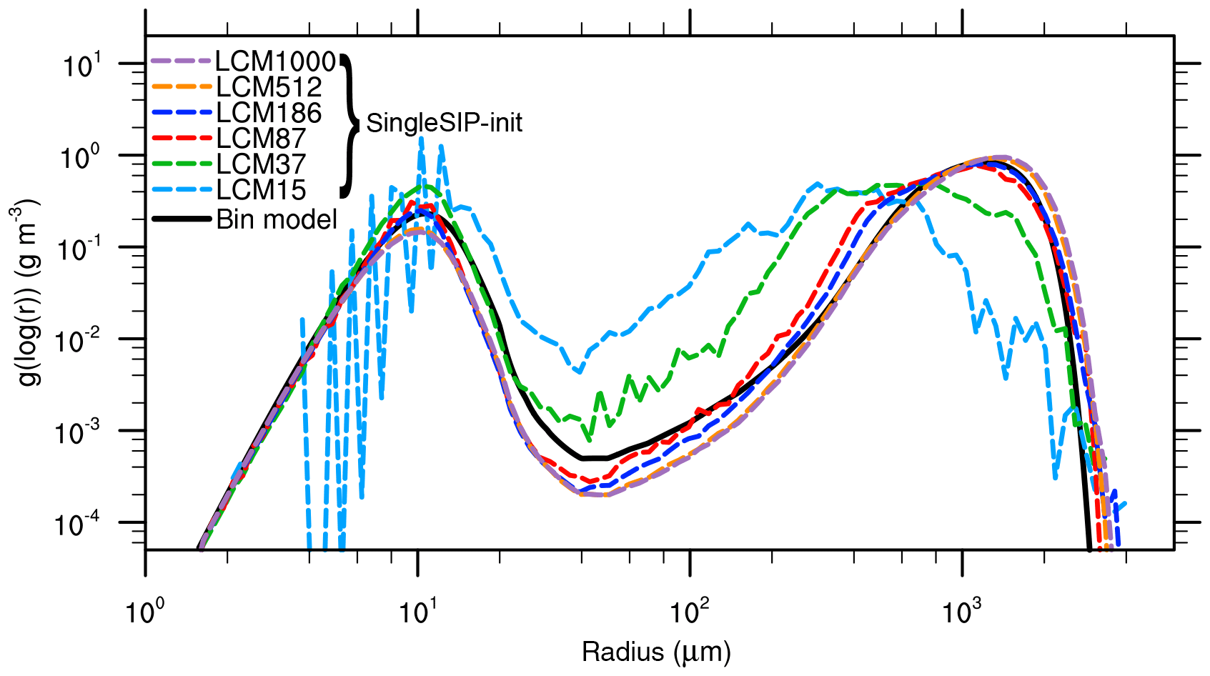
Figure 1Mass density distribution for the single-box approach after 3600 s for the “singleSIP” initialization. The black solid line denotes the solution of Wang et al. (2007). The colored dashed curves show the solution of the LCM with different numbers of superdroplets per grid box.
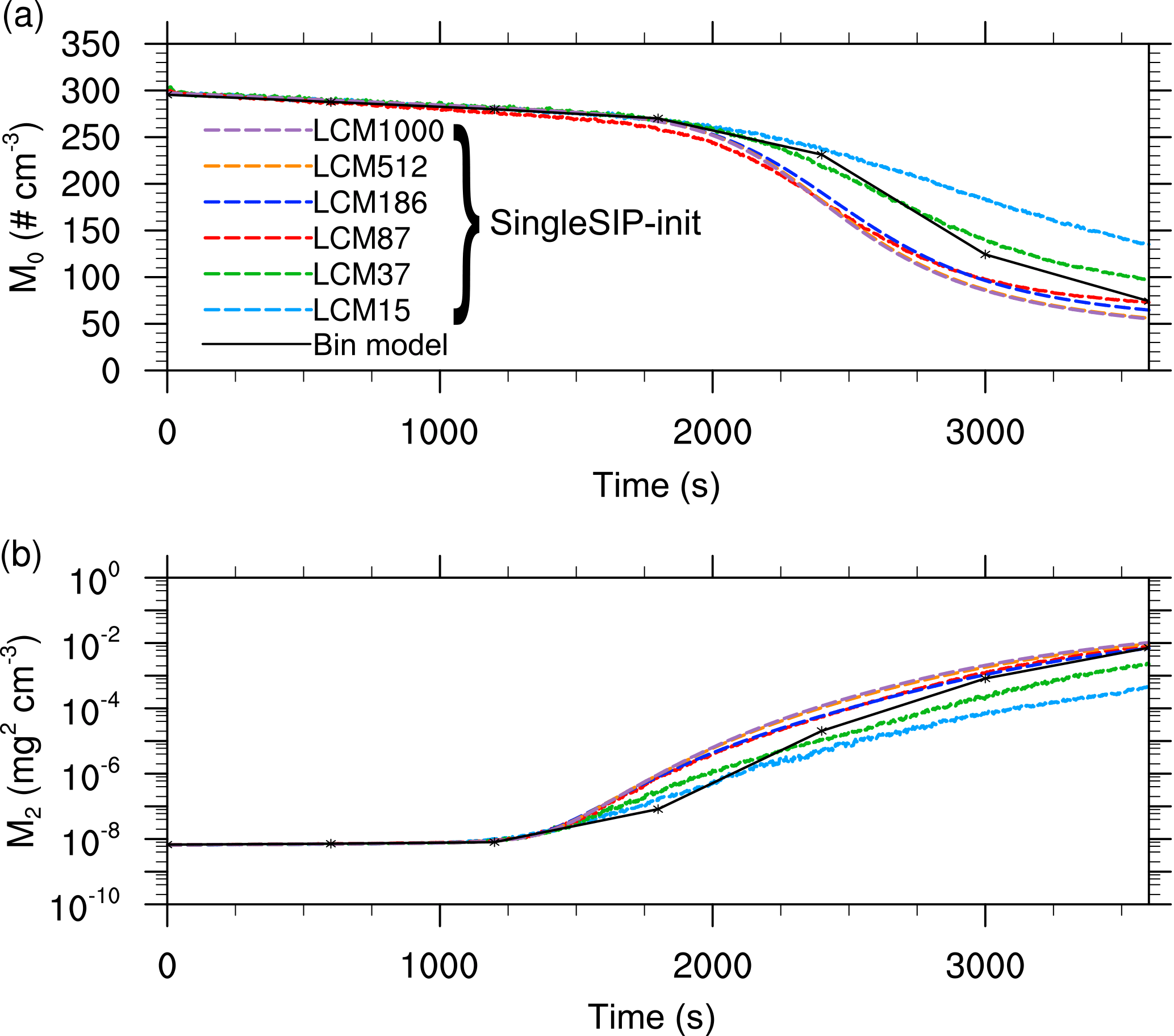
Figure 2Moments of the mass density distribution as a function of time obtained from the single-box simulations for the “singleSIP” initialization. The black solid line denotes the solution of Wang et al. (2007). The colored dashed curves show the solution of the LCM with different numbers of superdroplets per grid box.
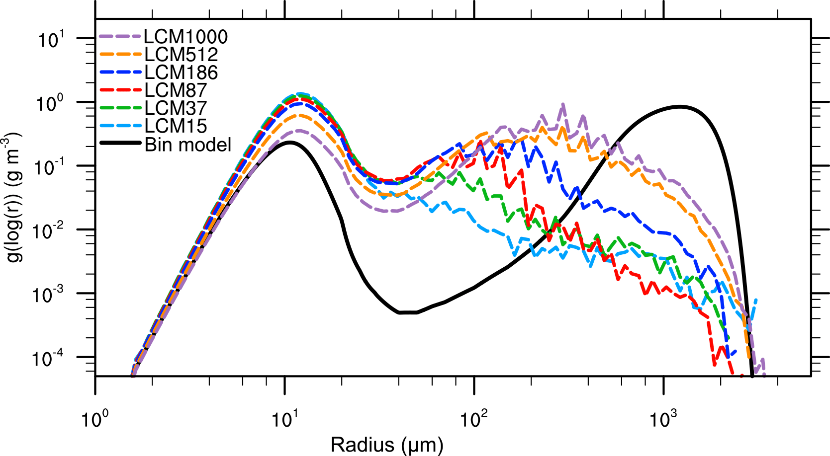
Figure 3Mass density distribution for the single-box approach after 3600 s. The black solid line denotes the solution of Wang et al. (2007). The colored dashed curves show the solution of the LCM with different numbers of superdroplets per grid box.
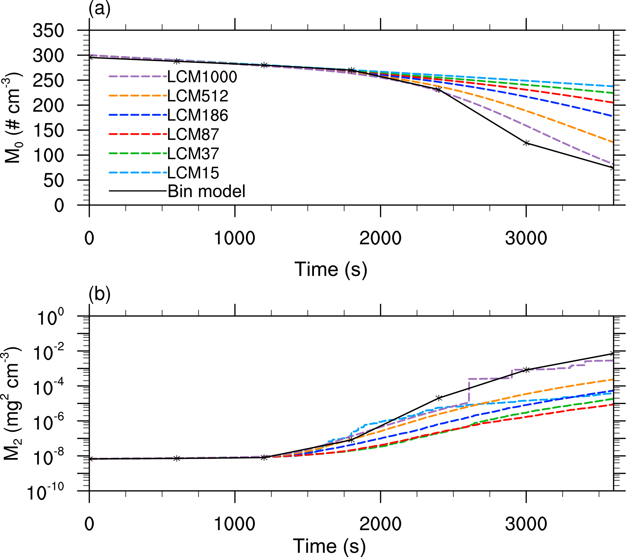
Figure 4Moments of the mass density distribution as a function of time obtained from the single-box simulations. The black solid line denotes the solution of Wang et al. (2007). The colored dashed curves show the solution of the LCM with different numbers of superdroplets per grid box.
Now, Figs. 3 and 4 show the same quantities but for the initialization with identical weighting factors. In Fig. 3, a significant deviation of the mass density distribution of the reference solution can be seen for all configurations. An excessively pronounced first maximum is found for all superdroplet concentrations, while the second maximum is at too small droplet sizes. Also, fluctuations occur for radii larger than 100 µm, resulting from insufficient superdroplet statistics in this range. However, as the initial number of superdroplets increases, the depletion of the first maximum and the development of the second maximum is reproduced better. Figure 4a shows that in all cases the decrease in the number concentration is underestimated. Also for the second moment (Fig. 4b), values are predicted too low in nearly all cases. All in all, it can be observed that an increase in the number of superdroplets leads to a better agreement of the results with the bin model even though difference are still significant for 1000 superdroplets per grid box.

Figure 5Mass density distribution for the single-box approach after 3600 s. The black solid line denotes the solution of Wang et al. (2007), the black dashed curve the reference case (without splitting). The colored dashed curves show solution for splitting simulation with different configurations.
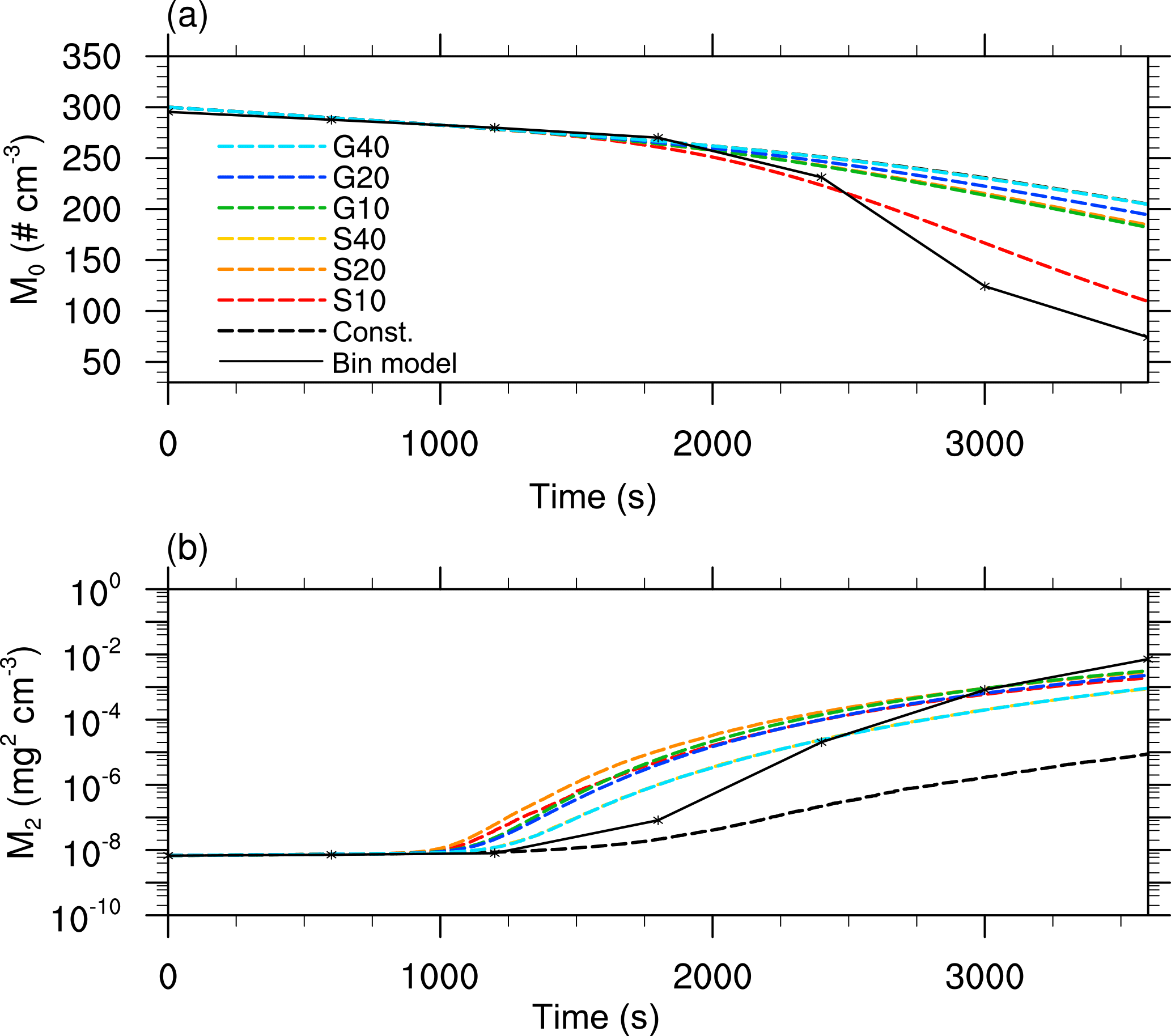
Figure 6Moments of the mass density distribution as a function of time obtained from single-box simulations. The black solid line denotes the solution of Wang et al. (2007), the black dashed curve for the reference simulation (without splitting). The colored dashed curves show the solutions for different splitting configurations.
In Figs. 5 and 6 the mass density distribution after 3600 s and the temporal development of the moments applying the splitting algorithm in different configurations are shown. Again, the splitting modes are abbreviated with S for the simple splitting method and G for using the splitting method based on a gamma distribution. The number following S or G indicates the splitting radius in microns. For all simulations, the maximum permissible number of superdroplets per grid box is limited to NP,max=1000. The maximum splitting factor is ηmax=20. By selecting these limits, which are chosen to represent the upper limit of computationally feasible three-dimensional simulations, it is possible to obtain an estimate of the quality of the individual splitting methods. The influence of the choice of these parameters is discussed below. All simulations are initialized with NP=87 superdroplets per grid box.
The black dashed line (Const.) shows the reference LCM case in which no splitting is applied. Comparing the non-splitting case to splitting cases, the results are significantly improved with respect to the reference solution. More precisely, the fluctuations that occur for large droplet radii are successfully removed by splitting. Furthermore, a better representation of the second maximum is also achieved by splitting. Independent of the splitting mode, simulations with the same splitting radius provide similar results. The only exception is between the simulations G10 and S10, in which the assumed gamma distribution enables effective splitting at slightly larger radii in G10 compared to S10. This results in a better agreement of S10 with the bin reference. In general, a reduction of the splitting radius leads to an improved representation of the mass density distribution. However, for all splitting simulations the reduction of the first maximum is underestimated, while the second maximum is only inadequately represented.
Similar conclusions are possible from Fig. 6, in which the time series of the zeroth and second moment of the DSD are shown. The best agreement for the number concentration is achieved by S10, where many superdroplets are cloned at a very early stage. For all splitting configurations, the second moment shows a strong improvement in comparison to the LCM reference case without splitting (Const.) where this value is largely underestimated. Accordingly, splitting leads to an improved representation of the collisional growth in LCMs but there are still very large deviations from the bin reference.
These results exhibit how strongly collisional growth suffers from the initialization with a constant weighting factor, consistent with Unterstrasser et al. (2017). Since large superdroplets are initialized only in a few grid boxes, collisional growth is subject to a great variability in the different realizations among the ensemble. Due to that, the following subsection will repeat this investigations using the multi-box approach, which reflects the collisional growth in 3-D applications more appropriately.

Figure 7Same as Fig. 3 but for the multi-box approach, i.e., interactions between the grid boxes are possible.
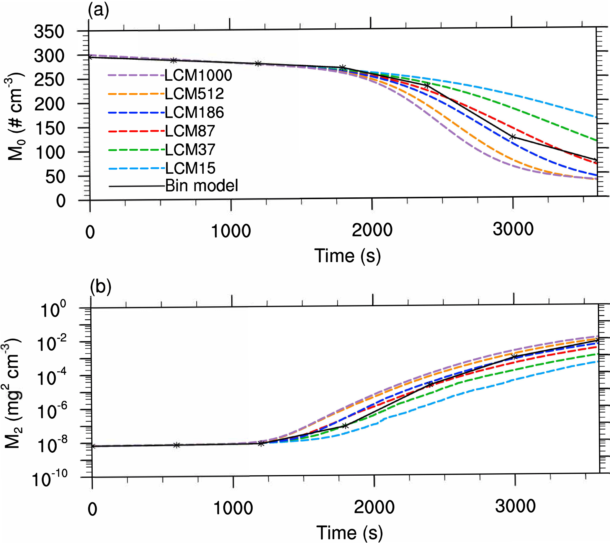
Figure 8Same as Fig. 4 but for the multi-box approach, i.e., interactions between the grid boxes are possible.
Multi-box approach
Figure 7 shows the mass density distribution after 3600 s time for different numbers of superdroplets (colored lines) using the multi-box approach without splitting. One can see that as the number of superdroplets increases, a better agreement with the bin model is achieved. Especially the simulations with 512 and 1000 superdroplets per grid box can reproduce the mass density distribution well. However, for these cases, a stronger decrease in the first maximum is observed. This can be attributed to accelerated accretion, which is favored by the combination of a few large droplets with an overestimated weighting factor and a large number of superdroplets with radii of about 10 µm. In contrast, a decelerated depletion of the first maximum and a weaker second peak are detected for simulations with a lower number of superdroplets. This results from the insufficient representation of the initial DSD, especially that of large droplets, which are crucial for effective collisional growth.
In Fig. 8, the temporal evolution of the number concentration and the second moment are shown. In simulations with a high number of superdroplets, a too strong reduction of the number concentration is predicted; and contrarily, the decrease in the zeroth moment is underestimated in cases with only 15 and 37 superdroplets. This tendency is also observed for the second moment. Simulations with a high number of superdroplets overestimate the reference, whereas simulations with only a few superdroplets result in too low values. However, comparing the results of the non-splitting cases (Const.) in the single- and multi-box simulations, the latter already provides improved results with respect to the bin model. The results show that this initialization artifact can be successfully mitigated by the newly introduced stochastic exchange between the grid boxes. For typical applications, however, the required amount of at least 512 superdroplets per grid box, necessary to derive satisfying results without splitting, is computationally unfeasible.
To maintain a reasonable amount of superdroplets, these box simulations will be repeated now, using the splitting approach. Here all parameters (initializing all simulations with 87 superdroplets per grid box) and splitting thresholds are identical as for the single-box approach described above but the superdroplets are now allowed to move between grid boxes.
Figure 9 shows the mass density distribution after 3600 s for different splitting configurations. Clear differences in the consistency with the bin reference solution can be seen. In particular, the simulations S10 and G10 show a good agreement with the results of Wang et al. (2007). In both cases, the bimodal shape of the spectrum is represented well. However, for the other simulations, the deviation from the reference solution increases with increasing splitting radius, but less with the splitting mode. Both simulations with a splitting radius of 40 µm show no improvements in comparison to a simulation without splitting (Const., black dashed line), except in the right tail of the distribution. Figure 10 shows the moments for the different splitting configurations. The two plots indicate a slightly faster precipitation process than in the bin model, but the general agreement with the reference is much higher than without splitting (Fig. 8). Again, general differences between the bin model and the LCM are caused by the initialization, which cannot be fixed by splitting. The initialization with constant weighting factors will always deviate from the exponential initialization used by Wang et al. (2007). Therefore, subsequent collisions, which are improved by splitting, cannot agree with the bin solution by Wang et al. (2007) whatsoever. In general, the decreasing difference among the different LCM simulations, as it is occurring due to splitting, needs to be seen as a proof of concept, and not the comparison with the bin results.
All in all, it is shown that collisional growth is better represented by using the splitting method in both the single- and multi-box simulations. Furthermore, the choice of the splitting mode is secondary, but the splitting radius is identified as the most crucial parameter. The multi-box simulations exhibit a distinct advantage over the single-box simulations. Due to the presence or absence of sufficiently large droplets that might initiate collision and coalescence, as a result of the initialization, collisional growth can be overestimated in certain grid boxes while it is underestimated in others. Splitting and the subsequent stochastic exchange are able to distribute these so-called precipitation embryos among the entire ensemble where they are able to initiate collision and coalescence as sketched in Fig. 11, which would not be possible in the single-box approach.
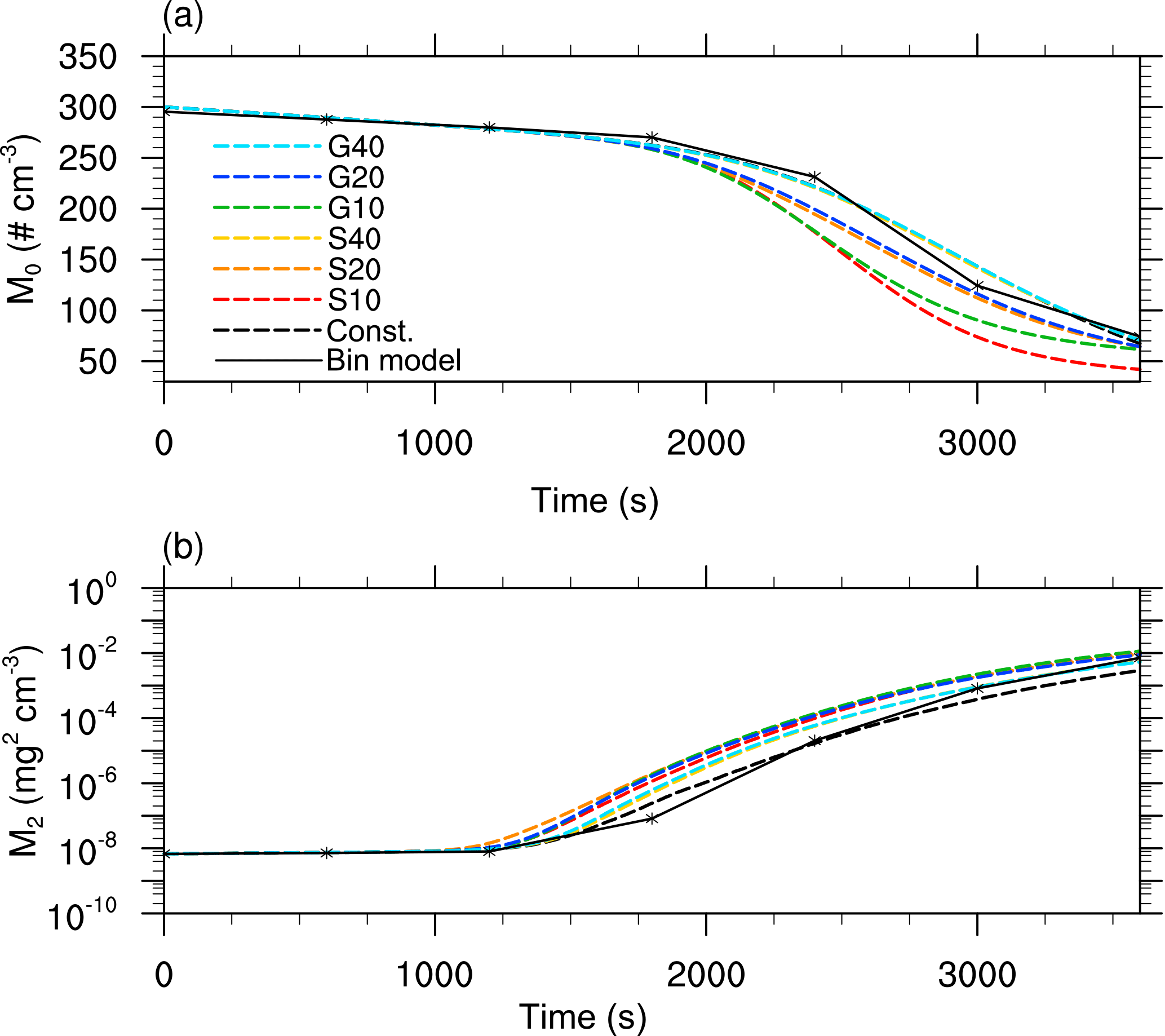
Figure 10Same as Fig. 6 but for the multi-box approach, i.e., interactions between the grid boxes are possible.
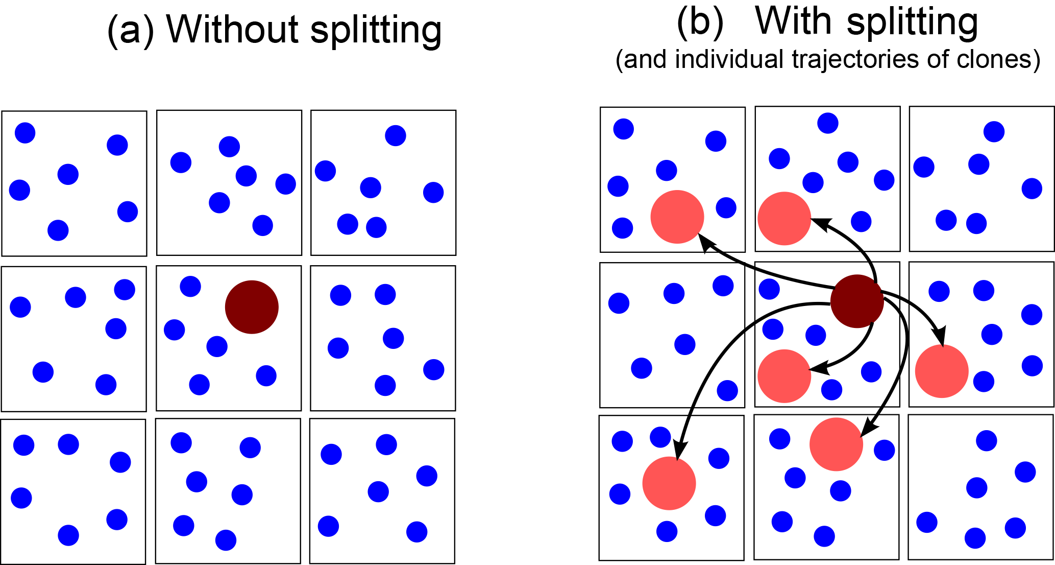
Figure 11Schematic representation on how splitting affects the spatial distribution of large superdroplets. The squares outline the different grid boxes with superdroplets of the size of cloud droplets (blue) and superdroplets representing rain drops (dark red). Without splitting (a), the rain drop is represented by only one superdroplet. In the splitting case with the multi-box approach (b), this superdroplet is cloned into several superdroplets, which are able to move in other grid boxes (due to their individual subgrid-scale velocities) where they initiate or affect collisional growth.
Sensitivity to splitting thresholds
The limiting parameters of the splitting algorithm are now examined in sensitivity studies using the multi-box approach. For this purpose, the parameters of the maximum possible number of superdroplets per grid box NP,max, the maximum splitting factor ηmax, and the splitting radius rspl are varied for the splitting mode G; the base state of this mode is defined as rspl=10 µm, ηmax=20, and NP,max=1000. This base state is varied by individually changing the parameters rspl, ηmax, and NP,max. Furthermore, all simulation are identically initialized with Ninit=87 superdroplets per grid box.
Figure 12a shows the mass density distributions after 3600 s for different values for NP,max. We find that a value of NP,max=150 is sufficient to reach convergence for this setup. Since the initial superdroplet concentration is Ninit=87 for all configurations of NP,max, it can be concluded that NP,max is a necessary but not crucial parameter as long as NP,max ⩾ 150. This reduction of the maximum number of superdroplets per grid box results in a reduction of the computational time by a factor of 15 compared to the simulation with NP,max=1000.
The sensitivity studies for the maximum splitting factor show that this has no influence on the results (Fig. 12b). An explanation for this is that the algorithm is executed at every time step and thus only the clone rate but not the absolute number of the clones is affected. More precisely, a low value of ηmax may reduce how many clones are produced at a time step. However, results show that this effect is negligible since a superdroplet will be cloned sufficiently fast at the subsequent time steps as long as NP≤NP,max.
As shown before, the development of the spectrum is highly sensitive to the choice of the splitting radius. Figure 12c shows that the results converge with decreasing splitting radius, with no significant deviations for configurations with rspl≤15 µm. This can be attributed to the fact that especially the largest droplets (in this case with radii of approximately 15 µm) are crucial for initiating the collisional growth. Accordingly, an improved representation of these droplets leads to an improved representation of the whole collisional growth process.
4.2 Single cloud
4.2.1 Setup
In this case, we are simulating an idealized shallow cumulus cloud in the form of a rising warm air bubble as in Hoffmann et al. (2017). The model domain is in the x-, y-, and z-direction, respectively. An isotropic grid spacing of 20 m is used. The simulation time is 3000 s using a constant time step of 0.1 s. The warm air bubble is triggered by a Gaussian-shaped potential temperature perturbation θ*
where θ0=0.4 K is the maximum temperature difference, which decreases with a standard deviation of σy=200 m and σz=150 m in the y- and z-direction, respectively. The center of the bubble is set to yc=3840 m and zc=170 m. Due to the two-dimensional character of the temperature excess, the initial temperature perturbation is elongated homogeneously along the x axis.

Figure 12Mass density distribution for the box simulation after 3600 s. The black solid line denotes the solution of Wang et al. (2007). In (a), sensitivity studies for different values of NP,max are presented. In (b), simulations for different values of ηmax are shown. In (c), results for different splitting radii are displayed. All sensitivity studies are conducted using the splitting mode G.
The initial profiles for temperature and specific humidity are based on the shallow cumulus case by vanZanten et al. (2011). Note that no background winds, large-scale forcings, or surface fluxes are considered. The superdroplets are released at the beginning of the simulation and are uniformly distributed in the entire model domain. For all three directions in space, the average distance of the superdroplets is initially 4.5 m. This results in a superdroplet concentration of approximately 87 superdroplets per grid box and roughly 4.55×10⁸ superdroplets in total. Using a weighting factor of , an initial cloud condensation nuclei (CCN) concentration of 100 cm−3 is represented. Additionally, simulations with 15 and 186 superdroplets per grid box are carried out, in which the weighting factor is adjusted such that the CCN concentration of 100 cm−3 is retained. If merging is applied, only superdroplets with a radius smaller than rmer=0.1 µm and with a weighting factor smaller than are allowed to merge.
At the surface, superdroplets are absorbed if their radius is larger than 1.0 µm. For smaller particles, a reflection boundary condition is assumed to avoid the change that the surface acts as a CCN sink. Horizontal boundaries are prescribed with cyclic conditions. Moreover, for collision and coalescence, the kernel by Hall (1980) is used. An overview of all conducted simulations is given in Table 1.
Table 1Summary of the main parameters for the single-cloud simulations.

4.2.2 Single-cloud results
Microphysical properties
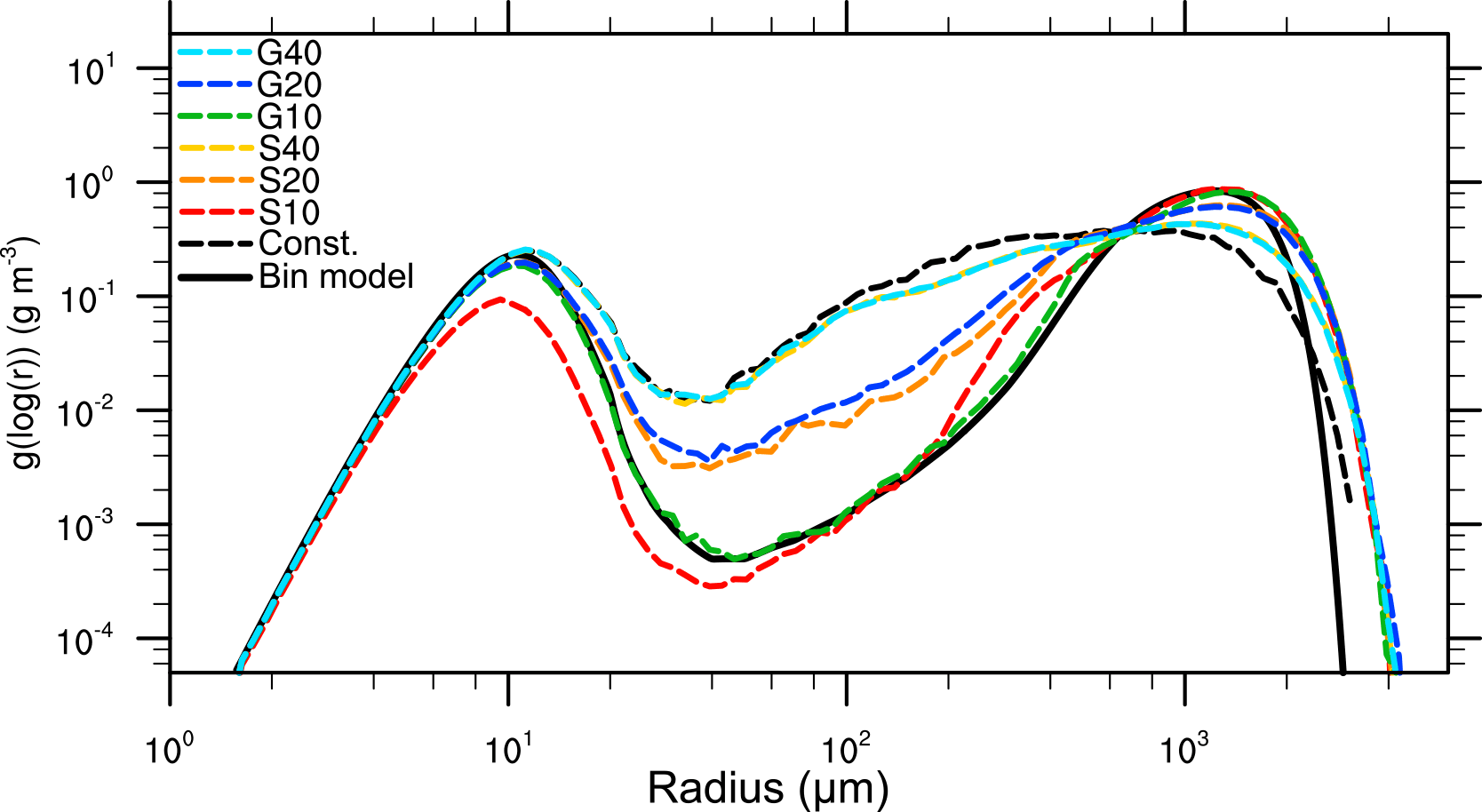
Figure 13 shows the cloud-averaged mass density distribution at t=1800 s for the configurations listed in Table 1. The left part of the spectrum is reproduced quantitatively consistent in all cases. This implies that both the splitting and the merging processes have no artificial impact on the diffusional growth process, which prevails in this region of the spectrum. However, the right tail of the DSDs differs significantly when the splitting algorithm is applied. The biggest drops are almost 350 µm smaller for the reference case (black lines) compared to simulations with splitting. Furthermore, splitting effectively reduces the fluctuations which occur in the reference cases for radii above 100 µm. The mass density distributions imply that the choice of the splitting mode does not affect cloud microphysical results. Likewise, the simulation S10, in which the splitting radius is reduced to rspl=10 µm, shows almost no difference in the mass density distribution compared to cases with rspl=20 µm. Thus, it can be deduced that a splitting radius of rspl=20 µm is sufficient for this cloud. Further investigations (not shown) in which rspl is successively increased to 30 µm show that a larger splitting radius leads to strong deviations from simulations with smaller splitting radii. This indicates that droplets with radii larger than 20 µm need to be represented in a statistically sufficient way to initiate the precipitation process correctly. It should be emphasized, however, that these results are only valid for a cloud with a relatively strong diffusional radius growth. A reduction of the splitting radius might be required for settings in which collisions dominate the droplet's growth at smaller radii as it is the case in the previously presented box simulations.
This behavior can be ascribed to different requirements on the superdroplet number for the convergence of different growth processes. The left part of the spectrum is dominated by diffusional growth which can be sufficiently represented by just a couple of superdroplets per grid box. By contrast, collisional growth is highly sensitive to the superdroplet number and the correct representation of large droplets. An improved representation of these droplets is ensured by the splitting algorithm, no matter what splitting mode is used.
The improved statistics of large superdroplets are also shown in Fig. 14, where the absolute number of superdroplets per logarithmic radius (log (r)) bin is presented. It is noticeable that in the reference simulations, this number decreases significantly for larger droplets (starting from a radius of approximately r=20 µm). In simulations in which no splitting operations are carried out, the largest droplets are represented by only a few tens of superdroplets in the whole model domain. For the S mode, the superdroplet concentration is kept almost constant (except in the right tail) for all splitting cases. For the G mode, a second maximum at 100 µm can be observed. This can be related to the calculation of the splitting criterion. The approximation of the mass density distribution by a gamma distribution results in a somewhat lower splitting factor for superdroplets close to the splitting radius in comparison to the S mode, which shifts the superdroplet production to larger radii in the G mode.
Macrophysical properties
In Fig. 15, the development of the cloud is shown in a time series of several macroscopic properties. The behavior of the different splitting configurations can be clearly seen in Fig. 15a, which depicts the ratio of the current superdroplet number to its initial value. In simulations without splitting, the superdroplet number remains nearly constant. A clear increase in the superdroplet number can be observed when splitting is used, with maximum increase of about 15 % for S10. In all other splitting cases, the increase in superdroplet number is notably lower and starts approximately 500 s later, which corresponds to the larger splitting radius of rspl=20 µm. The lowest increase in superdroplet number is observed in the merging cases in which the maximum number of superdroplets is reached during the growing phase of the cloud and decreases in the dissipation stage.

Figure 14Total number of superdroplets per logarithmic radius bin after t=1800 s for the idealized single-cloud simulations using parameters described in Table 1.
Figure 15b and c show the temporal evolution of the liquid water path (LWP) and the rain water path (RWP). The RWP is defined as the integral mass of all droplets with r≥40 µm. It is notable that the LWP is the same for all simulations, which emphasizes the mass-conserving character of the splitting algorithm and its negligible impact on the general development of the cloud. In the reference simulations (represented as a mean of five ensembles for each case) of Figs. 15c and d, one can see an increase in the precipitation parameters (RWP, radar reflectivity, and precipitation sum) for an increased number of superdroplets. However, the differences among the ensemble members are quite large, which is shown by the range (gray area) and the band of plus–minus one standard deviation from the mean (light blue area) derived from all 15 ensemble members. Overall, the splitting simulations have a slight tendency to compare better with the reference cases using 87 and 186 superdroplets. Admittedly, since the results are (for the most part) within one standard deviation, it can be concluded that splitting has no significant influence on the global precipitation parameters.
Figure 15e and f display the precipitation rate and the total precipitation reaching the ground. The precipitation rate in the reference simulations without splitting exhibit high temporal variances (black lines). Those variances are successfully reduced in all splitting simulations. This can be explained by the better representation of precipitation in the splitting simulations by a larger number of superdroplets, resulting in a more uniform removal of liquid water by precipitation. As expected from the RWP, splitting slightly increases the total precipitation.
Figure 16 shows the effect of splitting on the spatial distribution of rain after 2100 s simulated time for the NP87 simulation (Fig. 16a) and the S20 splitting simulation (Fig. 16b). Similar to the reduced temporal variance in the time series of the precipitation rate (Fig. 15e), the spatial variance is also significantly reduced using splitting. Again, the precipitation is represented by only a few superdroplets in the simulation without splitting, which leads to very high, localized precipitation rates. Due to splitting, raindrops with large weighting factors are split into several superdroplets with smaller weighting factors, resulting in the more realistic spatial representation of the precipitation.
All in all, the splitting of large droplets, which results in an improved representation of the collision process and thus the DSD, also partly influences the macroscopic properties of the cloud. In particular, rain water content, radar reflectivity, and precipitation rate are represented in a more realistic manner. Due to the improved statistics, the temporal and spatial variance of these parameters is significantly reduced. However, the whole cloud life cycle, which is driven by the general dynamics and thermodynamics, is largely unaffected by splitting. Additionally, the merging shows no influence on the physical outcomes.
To estimate the increase in computing time due to splitting, we conducted three simulations (Const. NP87, S20, and S20 merging) with comparable time measurements. Here we observe that the splitting simulation S20 requires 19.2 % more computing time than the reference simulation Const. NP87. If applied, merging allows a massive reduction of the number of superdroplets, reducing the computing time by 18 % and the storage demand (which is proportional to the number of superdroplets) by at least 7 % compared to simulations applying only splitting (Fig. 15a). All in all, the simulation applying both splitting and merging is only 1.2% slower than the reference simulation Const. NP87.
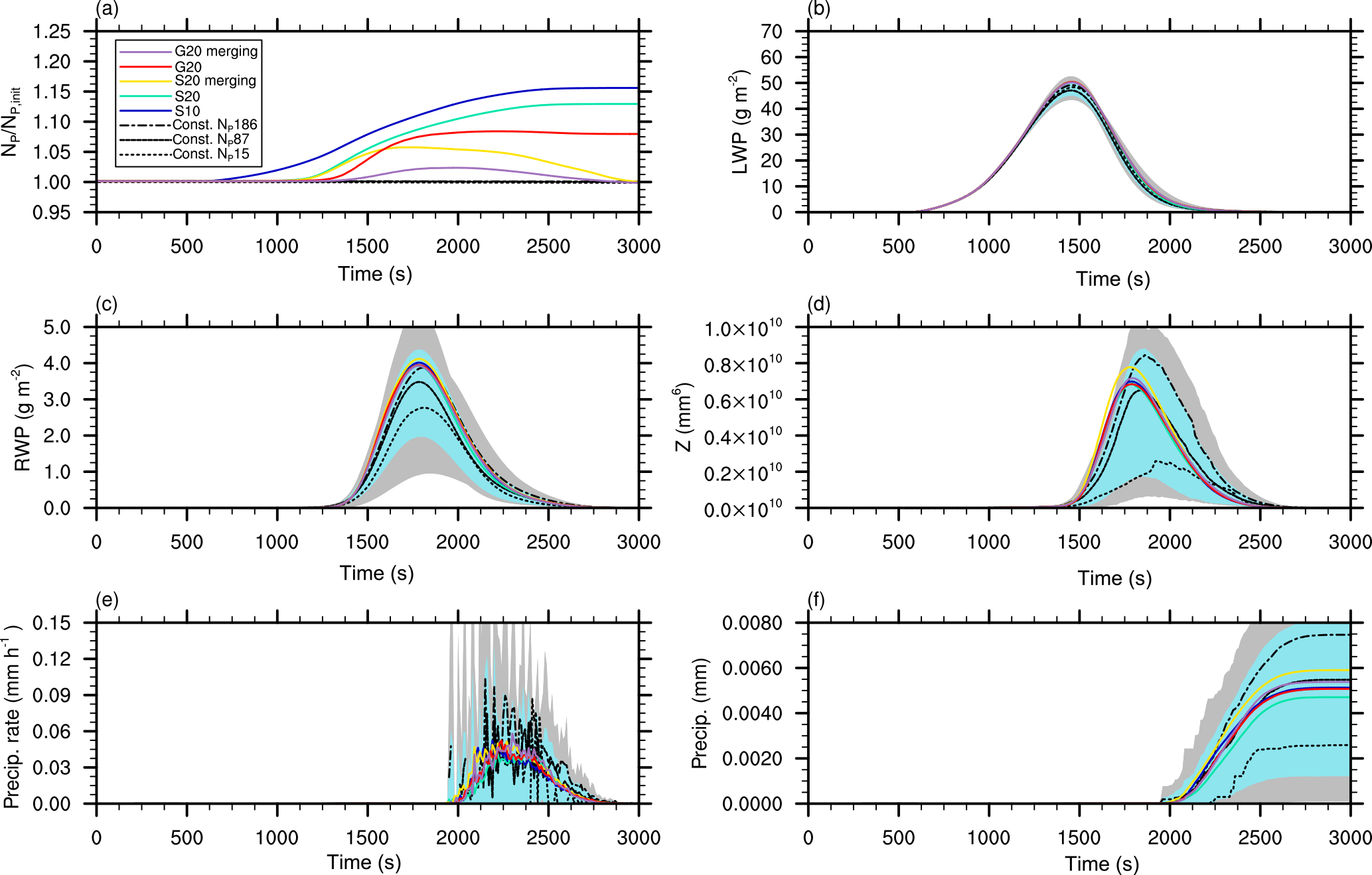
Figure 15Time series of different variables for the idealized single-cloud simulation for different initial numbers of superdroplets and splitting configurations. In (a), the ratio of the actual and initialized number of superdroplets in the whole model domain is shown. The liquid water path (LWP) and rainwater path (RWP) are displayed in panels (b) and (c), respectively. In (d), the total radar reflectivity is shown. Panels (e) and (f) show the precipitation rate and total precipitation, respectively. The reference simulations (runs without splitting) are presented as a mean of five ensembles for each case. Moreover, the light blue areas show the mean plus–minus one standard deviation and the gray areas show the range derived from all 15 ensemble members.
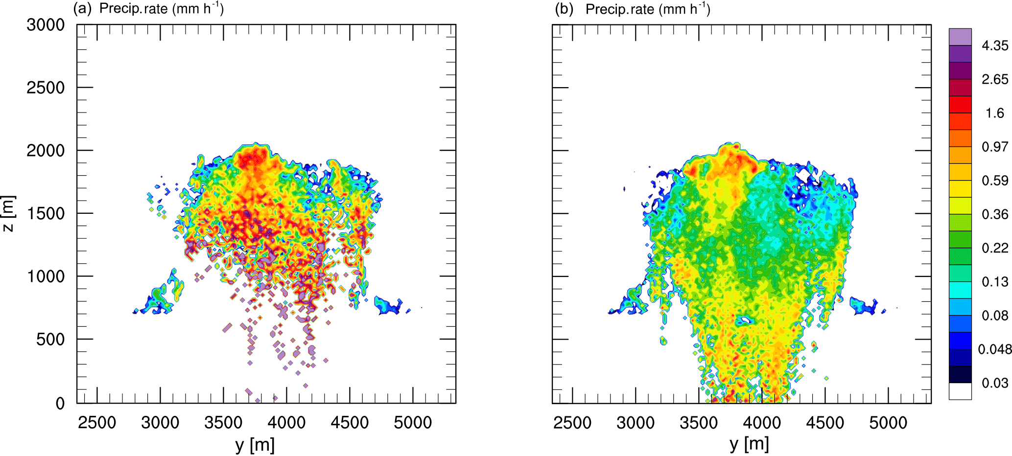
Figure 16Vertical cross sections of the precipitation rate for the reference case (a) and the splitting case S20 (b).
4.3 Cloud field
4.3.1 Setup
The setup for simulating a shallow cumulus field is based on the LES intercomparison study by vanZanten et al. (2011), using their initial profiles for potential temperature, water vapor mixing ratio, large-scale forcings, and surface fluxes. As in the original, the model domain covers an area of about in the x-, y-, and z-direction, respectively. The grid spacing is in the horizontal, and Δz=40 m in the vertical. Moreover, the calculation of the domain-averaged quantities follows the descriptions given in the original case.
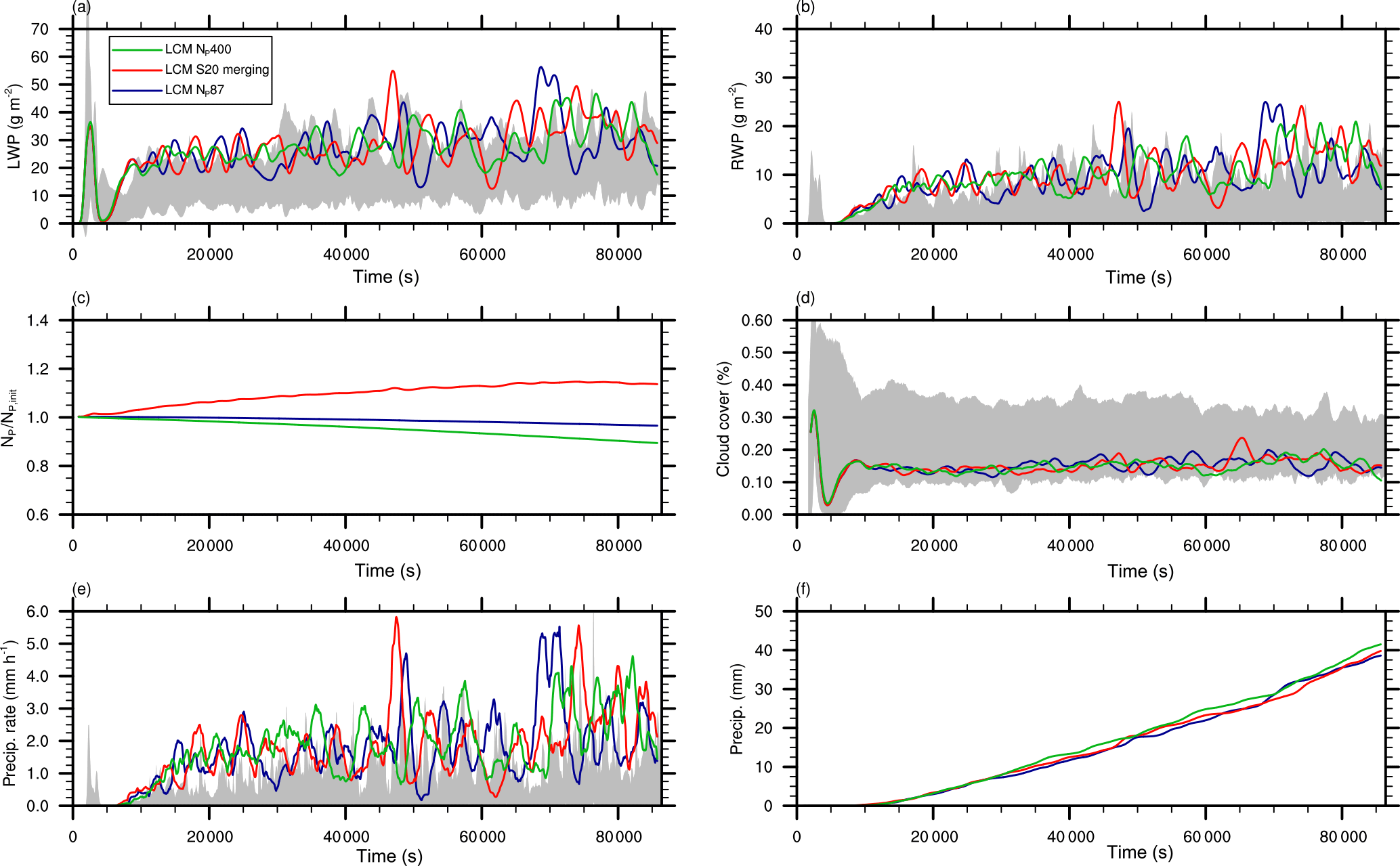
Figure 17Time series of (a) the liquid water path (LWP), (b) rainwater path (RWP), (c) ratio of the actual number of superdroplets to the initial number of superdroplets, (d) cloud cover, (e) precipitation rate, and (f) total precipitation for different initial numbers of superdroplets and splitting configurations. The gray areas in (a), (b), and (d) indicate the documented model variability in the simulated shallow cumulus case (vanZanten et al., 2011).
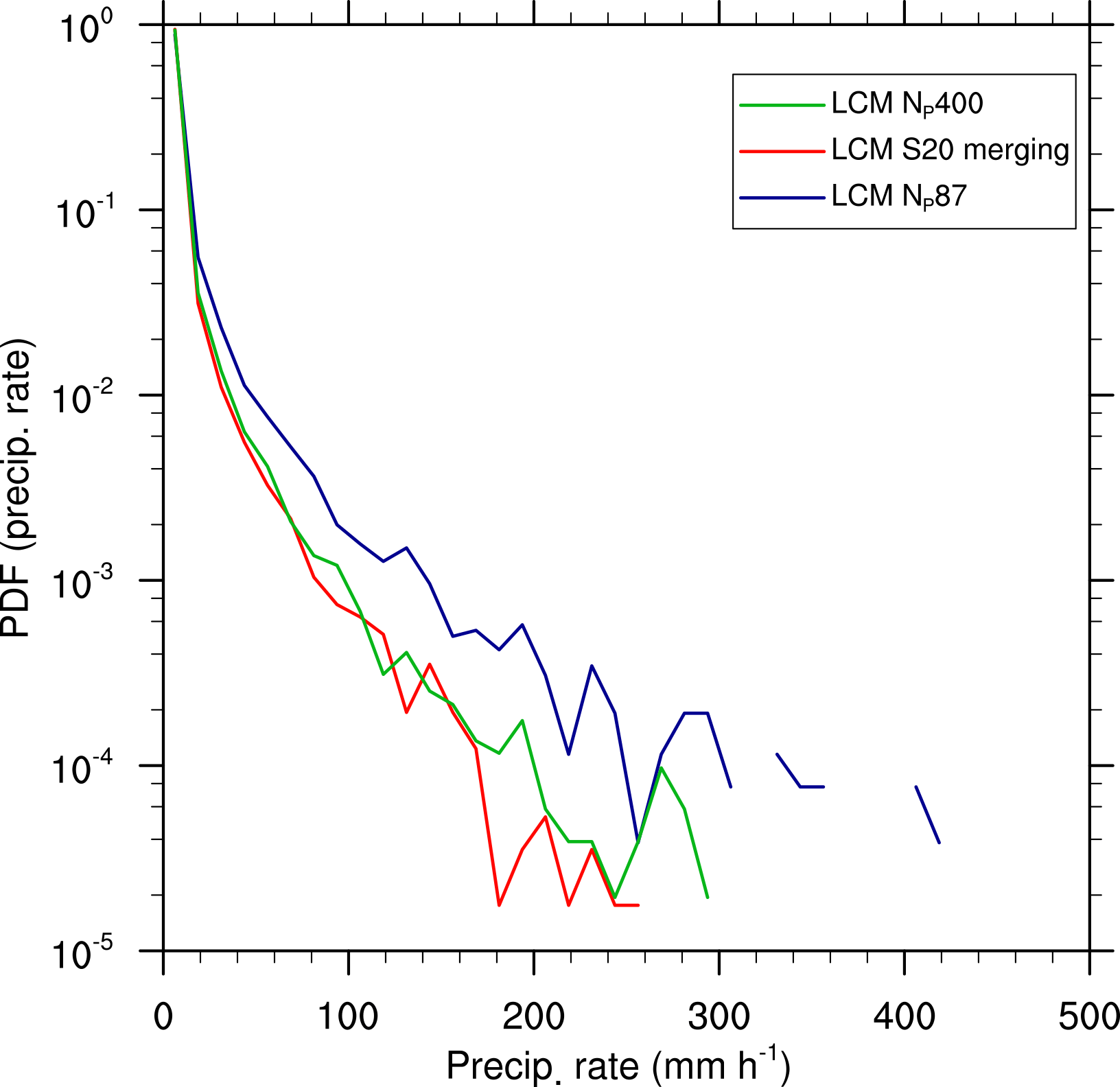
Figure 18Probability density function of precipitation rates for different initial numbers of superdroplets and splitting configurations.
Three different simulations will be presented. In the cases LCM NP87 and LCM NP400, the number of superdroplets per grid box are 87 and 400, respectively. With initial weighting factors of and , respectively; these represent a CCN concentration of 100 cm−3 in each case. Moreover, one more simulation with splitting and merging is carried out. For this configuration, in which the general settings of LCM NP87 are adopted, the splitting mode S with rspl=20 µm, ηspl=20, and is used. Aspl is chosen to allow number concentrations as small as 1 m−3 to be represent by a single superdroplet.
Based on the previously presented results, the maximum number of particles per grid box is set to NP,max=150. Merging is applied in non-cloudy grid boxes for superdroplets with a radius smaller than rmer=0.1 µm and a weighting factor smaller than .
4.3.2 Cloud field results
The analysis is focused on the influence of splitting on the macroscopic properties of the shallow cumulus field. Figure 17 shows time series of (a) the LWP, (b) RWP, (c) ratio of the current superdroplet number to its initial value, (d) cloud cover, (e) precipitation rate, and (f) total precipitation. Despite the superdroplet number, all these parameters agree in a statistical sense. In the cases without splitting, the total superdroplet number decreases slightly in the course of the simulation due to precipitation (Fig. 17c), while the simulation with splitting increases the total superdroplet number by about 15 %. Note, however, that both LWP and RWP are at the top of model variability documented in vanZanten et al. (2011) (gray areas), which is in line with the results of Arabas and Shima (2013), who also used an LCM for the simulation of this shallow cumulus case.
Considering the temporal variability in the precipitation rate and total precipitation (Fig. 17e and f), no significant changes are detectable using splitting or a very high number of superdroplets. Nonetheless, a positive impact of splitting on the representation of precipitation can be seen in the probability density function of the surface precipitation rate (Fig. 18). For the simulation with 400 superdroplets per grid box and the splitting simulation, the probability for very high precipitation rates is smaller by about 1 order of magnitude compared to the simulation LCM NP87. This clearly shows that extremely high precipitation rates, resulting from individual superdroplets with large weighting factors, are mitigated when splitting is applied. Accordingly, splitting is important for a statistically appropriate representation of individual rain events and necessary for the process-level understanding of the precipitation process, but the general features of the cloud field, as it was the case for the single cloud, are largely unaffected.
The main objective of this paper was the development and verification of a splitting algorithm to improve collisional growth in Lagrangian cloud models (LCMs). These models are able to represent collision and coalescence well (Unterstrasser et al., 2017; Dziekan and Pawlowska, 2017). Under certain conditions, however, they are known to insufficiently represent this process. These conditions occur when the number of superdroplets is low and, accordingly, the number of real droplets represented by each superdroplet (the so-called weighting factor) is high, leading to an oversimplified representation of the droplet size distribution (DSD; Riechelmann et al., 2012; Unterstrasser et al., 2017). The introduced approach for splitting is carried out by cloning superdroplets of interest (large radius and high weighting factor) into a large number of identical superdroplets with commensurately reduced weighting factors, which improves the representation of the DSD in the desired areas. An accompanying merging algorithm has been also introduced. It is designed to merge two superdroplets into one, counteracting the (potentially) massive production of superdroplets due to splitting and hence a significant increase in computational cost.
The splitting and merging algorithms have been validated using box simulations, a simulation of a single cumulus cloud, and an established shallow cumulus test case. The box simulations confirmed that the capability of an LCM to represent the temporal evolution of a DSD due to collision and coalescence depends crucially on the number of simulated superdroplets (Shima et al., 2009; Riechelmann et al., 2012; Unterstrasser et al., 2017; Dziekan and Pawlowska, 2017). Without splitting, only simulations with more than 500 to 1000 superdroplets per grid box were acceptably reproducing literature references. By applying the new splitting algorithm, the results improved significantly using only up to 150 superdroplets per grid box. Furthermore, the box simulations revealed that the radius from which splitting is applied is the most important parameter of the splitting algorithm. A value of 15 µm, which corresponds to the typical radii of the first colliding droplets in clouds, was found to be appropriate. Other investigated parameters have shown only a minor impact on the results as long as a sufficiently large maximum number of superdroplets is allowed to be produced by splitting (≥150).
In the idealized single-cloud simulation, splitting improved the representation of collisional growth with up to 70 % larger maximum radii. Moreover, splitting improves the spatial and temporal representation of precipitation by distributing the precipitable water on more superdroplets with an accordingly smaller weighting factor. It is important to note, however, that the life cycle and domain-averaged macroscopic properties are almost not affected by the splitting process. If applied, the merging algorithm has been shown to reduce the computing time by 18 % and the storage demand by at least 7 % in comparison to simulations with splitting alone. Since merging is restricted to cloud-free regions, its application did not alter the simulated physics. Similar findings on the effect of splitting on the production of rain have been made for the shallow cumulus test case.
In light of the fact that LCMs become increasingly important in the field of modeling cloud microphysics, it is necessary to minimize the (typically) large demand of memory and computing time required for their application. Thus, a fixed number of superdroplets needs to be replaced by a dynamic number, which adapts interactively to the given physical and numerical requirements. In this regard, the presented methods follow the approaches by Grabowski et al. (2018), in which superdroplets are only created after activation, or Naumann and Seifert (2015), who restricted the superdroplet approach to the representation of raindrops. Of course, all these approaches have their specific advantages and disadvantages, but they are necessary steps to apply LCMs in a wider range of future applications.
The LES model used in this study (revision 2263) is publicly available at https://palm.muk.uni-hannover.de/trac/browser/palm?rev=2263 (last access: 25 September 2018, PALM group, 2018). For analysis, the model has been extended and additional analysis tools have been developed. The extended code is available from the authors on request.
JS carried out the analysis. JS, FH, and SR developed the basic ideas, discussed the results, and wrote the manuscript.
The authors declare that they have no conflict of interest.
All simulations have been carried out on the Cray XC40 systems of the
North-German Supercomputing Alliance (HLRN, https://www.hlrn.de/, last
access: 25 September 2018).
The publication of
this article was funded by the open-access
fund of Leibniz
Universität Hannover.
Edited by: Holger
Tost
Reviewed by: two anonymous referees
Andrejczuk, M., Grabowski, W., Reisner, J., and Gadian, A.: Cloud-aerosol interactions for boundary layer stratocumulus in the Lagrangian Cloud Model, J. Geophys. Res., 115, D22214, https://doi.org/10.1029/2010JD014248, 2010. a, b
Arabas, S. and Shima, S.-I.: Large-eddy simulations of trade wind cumuli using particle-based microphysics with Monte Carlo coalescence, J. Atmos. Sci., 70, 2768–2777, 2013. a
Arabas, S., Jaruga, A., Pawlowska, H., and Grabowski, W. W.: libcloudph++ 1.0: a single-moment bulk, double-moment bulk, and particle-based warm-rain microphysics library in C++, Geosci. Model Dev., 8, 1677–1707, https://doi.org/10.5194/gmd-8-1677-2015, 2015. a, b
Dziekan, P. and Pawlowska, H.: Stochastic coalescence in Lagrangian cloud microphysics, Atmos. Chem. Phys., 17, 13509–13520, https://doi.org/10.5194/acp-17-13509-2017, 2017. a, b, c, d, e
Grabowski, W. W., Dziekan, P., and Pawlowska, H.: Lagrangian condensation microphysics with Twomey CCN activation, Geosci. Model Dev., 11, 103–120, https://doi.org/10.5194/gmd-11-103-2018, 2018. a, b
Hall, W. D.: A detailed microphysical model within a two-dimensional dynamic framework: Model description and preliminary results, J. Atmos. Sci., 37, 2486–2507, 1980. a, b
Hoffmann, F.: On the limits of Köhler activation theory: how do collision and coalescence affect the activation of aerosols?, Atmos. Chem. Phys., 17, 8343–8356, https://doi.org/10.5194/acp-17-8343-2017, 2017. a
Hoffmann, F., Raasch, S., and Noh, Y.: Entrainment of aerosols and their activation in a shallow cumulus cloud studied with a coupled LCM-LES approach, Atmos. Res., 156, 43–57, 2015. a
Hoffmann, F., Noh, Y., and Raasch, S.: The route to raindrop formation in a shallow cumulus cloud simulated by a Lagrangian cloud model, J. Atmos. Sci., 74, 2125–2142, 2017. a, b, c, d, e
Maronga, B., Gryschka, M., Heinze, R., Hoffmann, F., Kanani-Sühring, F., Keck, M., Ketelsen, K., Letzel, M. O., Sühring, M., and Raasch, S.: The Parallelized Large-Eddy Simulation Model (PALM) version 4.0 for atmospheric and oceanic flows: model formulation, recent developments, and future perspectives, Geosci. Model Dev., 8, 2515–2551, https://doi.org/10.5194/gmd-8-2515-2015, 2015. a
Naumann, A. K. and Seifert, A.: A Lagrangian drop model to study warm rain microphysical processes in shallow cumulus, J. Adv. Model. Earth Syst., 7, 1136–1154, 2015. a, b, c
Naumann, A. K. and Seifert, A.: Recirculation and growth of raindrops in simulated shallow cumulus, J. Adv. Model. Earth Syst., 8, 520–537, 2016. a
PALM group: The Parallelized Large-Eddy Simulation Model (PALM) –revision 2263, https://doi.org/10.25835/0044820, 2018. a
Riechelmann, T., Noh, Y., and Raasch, S.: A new method for large-eddy simulations of clouds with Lagrangian droplets including the effects of turbulent collision, New J. Phys., 14, 065008, https://doi.org/10.1088/1367-2630/14/6/065008, 2012. a, b, c, d, e, f
Rogers, R. R. and Yau, M. K.: A Short Course in Cloud Physics, Pergamon Press, New York, 1989. a, b
Sardina, G., Poulain, S., Brandt, L., and Caballero, R.: Broadening of Cloud Droplet Size Spectra by Stochastic Condensation: Effects of Mean Updraft Velocity and CCN Activation, J. Atmos. Sci., 75, 451–467, 2018. a, b
Seifert, A.: On the parameterization of evaporation of raindrops as simulated by a one-dimensional rainshaft model, J. Atmos. Sci., 65, 3608–3619, 2008. a
Shaw, R. A., Reade, W. C., Collins, L. R., and Verlinde, J.: Preferential concentration of cloud droplets by turbulence: Effects on the early evolution of cumulus cloud droplet spectra, J. Atmos. Sci., 55, 1965–1976, 1998. a
Shima, S., Kusano, K., Kawano, A., Sugiyama, T., and Kawahara, S.: The super-droplet method for the numerical simulation of clouds and precipitation: A particle-based and probabilistic microphysics model coupled with a non-hydrostatic model, Q. J. Roy. Meteor. Soc., 135, 1307–1320, 2009. a, b, c, d
Sölch, I. and Kärcher, B.: A large-eddy model for cirrus clouds with explicit aerosol and ice microphysics and Lagrangian ice particle tracking, Q. J. Roy. Meteor. Soc., 136, 2074–2093, 2010. a, b, c
Ulbrich, C. W.: Natural variations in the analytical form of the raindrop size distribution, J. Climate Appl. Meteor., 22, 1764–1775, 1983. a
Unterstrasser, S. and Sölch, I.: Optimisation of the simulation particle number in a Lagrangian ice microphysical model, Geosci. Model Dev., 7, 695–709, https://doi.org/10.5194/gmd-7-695-2014, 2014. a
Unterstrasser, S., Hoffmann, F., and Lerch, M.: Collection/aggregation algorithms in Lagrangian cloud microphysical models: rigorous evaluation in box model simulations, Geosci. Model Dev., 10, 1521–1548, https://doi.org/10.5194/gmd-10-1521-2017, 2017. a, b, c, d, e, f, g, h, i, j, k, l
vanZanten, M. C., Stevens, B., Nuijens, L., Siebesma, A. P., Ackerman, A. S., Burnet, F., Cheng, A., Couvreux, F., Jiang, H., Khairoutdinov, M., Kogan, Y., Lewellen, D. C., Mechem, D., Nakamura, K., Noda, A., Shipway, B. J., Slawinska, J., Wang, S., and Wyszogrodzki, A.: Controls on precipitation and cloudiness in simulations of trade-wind cumulus as observed during RICO, J. Adv. Model. Earth Syst., 3, M06001, https://doi.org/10.1029/2011MS000056, 2011. a, b, c, d
Wang, L.-P., Xue, Y., and Grabowski, W. W.: A bin integral method for solving the kinetic collection equation, J. Comput. Phys., 226, 59–88, 2007. a, b, c, d, e, f, g, h, i, j, k, l, m, n, o