the Creative Commons Attribution 4.0 License.
the Creative Commons Attribution 4.0 License.
 | 16 Oct 2018
Evaluating simplified chemical mechanisms within present-day simulations of the Community Earth System Model version 1.2 with CAM4 (CESM1.2 CAM-chem): MOZART-4 vs. Reduced Hydrocarbon vs. Super-Fast chemistry
Benjamin Brown-Steiner
Noelle E. Selin
Ronald Prinn
Simone Tilmes
Louisa Emmons
Jean-François Lamarque
Philip Cameron-Smith
While state-of-the-art complex chemical mechanisms expand our understanding of atmospheric chemistry, their sheer size and computational requirements often limit simulations to short lengths or ensembles to only a few members. Here we present and compare three 25-year present-day offline simulations with chemical mechanisms of different levels of complexity using the Community Earth System Model (CESM) Version 1.2 CAM-chem (CAM4): the Model for Ozone and Related Chemical Tracers, version 4 (MOZART-4) mechanism, the Reduced Hydrocarbon mechanism, and the Super-Fast mechanism. We show that, for most regions and time periods, differences in simulated ozone chemistry between these three mechanisms are smaller than the model–observation differences themselves. The MOZART-4 mechanism and the Reduced Hydrocarbon are in close agreement in their representation of ozone throughout the troposphere during all time periods (annual, seasonal, and diurnal). While the Super-Fast mechanism tends to have higher simulated ozone variability and differs from the MOZART-4 mechanism over regions of high biogenic emissions, it is surprisingly capable of simulating ozone adequately given its simplicity. We explore the trade-offs between chemical mechanism complexity and computational cost by identifying regions where the simpler mechanisms are comparable to the MOZART-4 mechanism and regions where they are not. The Super-Fast mechanism is 3 times as fast as the MOZART-4 mechanism, which allows for longer simulations or ensembles with more members that may not be feasible with the MOZART-4 mechanism given limited computational resources.
- Article
(6909 KB) -
Supplement
(696 KB) - BibTeX
- EndNote


The anthropogenic influence on atmospheric chemistry is apparent at all spatial and temporal scales: human emissions have impacted local and very short-lived species (e.g., OH; see Prinn et al., 2001), very long-lived greenhouse gases (e.g., Collins et al., 2006), and everything in between (e.g., Baker et al., 2015; Solomon et al., 2016). Over the past decades, all three branches of modern atmospheric chemistry research (Abbatt et al., 2014) – observations, laboratory analysis, and modeling – have increased in both their sophistication and their capability to explain the chemistry of our atmosphere. However, while observational networks have significant growth potential (e.g., Sofen et al., 2016) and laboratory analysis still has significant challenges to overcome (Bocquet et al., 2015; Burkholder et al., 2017), chemistry modeling efforts are finding their growth potential limited by the level of chemical complexity that can be included in models due to the constraint of the computational capabilities of even state-of-the-art supercomputers (Stockwell et al., 2012). Simulations that attempt to include all known species and reactions, such as the National Center for Atmospheric Research (NCAR) Master Mechanism (Madronich and Calvert, 1989; Aumont et al., 2000) or the Leeds Master Chemical Mechanism (Jenkin et al., 1997; Saunders et al., 2003) and even some species and reactions that have not been tested in any laboratory (e.g., Aumont et al., 2005; Szopa et al., 2005), are often limited to box-model-level analysis (e.g., Emmerson and Evans, 2009; Squire et al., 2015). Modeling efforts that simulate regional- and global-scale atmospheric chemistry are forced, out of practical necessity, to utilize simplified, reduced-form, and parameterized chemistry in order to address the large spatial and long temporal scales needed for policy-relevant research.
Historically, as computational capacity has increased, modeling efforts have tended to maximize model resolution and complexity. This limits the capability to perform multi-scenario or multi-model ensembles to institutions with access to significant computational capabilities and storage. One way to increase the number of scenarios or members in an ensemble is to reduce the complexity of the chemical mechanism. This selection of a reduced-form chemical mechanism for different applications and the advantages of the increased computational efficiency of a simplified mechanism are the main focus of this paper. While there is a long history of publications (see Dodge, 2000) that compare different photochemical mechanisms within box models (e.g., Milford et al., 1992; Jimenez et al., 2003; Emmerson and Evans, 2009; Knote et al., 2015), studies that compare multiple mechanisms within a single 3-D global model are rare (e.g., Squire et al., 2015). This study examines three chemical mechanisms within the Community Earth System Model Community Atmosphere Model with Chemistry Version 1.2 (CESM1.2 CAM-chem; Lamarque et al., 2012) framework: the Model for Ozone and Related Chemical Tracers, version 4 (MOZART-4) mechanism, the Reduced Hydrocarbon mechanism, and the Super-Fast chemical mechanism (described in Sect. 2), which is one of the simplest representations of atmospheric chemistry used within climate–chemistry model intercomparison projects, such as the Atmospheric Chemistry and Climate Model Intercomparison Project (ACCMIP; Lamarque et al., 2013).
This study examines the trade-offs and possibilities that arise from the selection of a chemical mechanism that is simple enough to be computationally efficient – and thus capable of long simulations or large ensembles at the global scale – as well as sophisticated enough to simulate the major features of tropospheric chemistry at the local and regional scale. Many climate studies include little to no chemistry or prescribed chemistry, even though chemistry–climate feedbacks are well established to impact global and regional climate (e.g., Marsh et al., 2013; Fiore et al., 2015). Indeed, coarse-grid () chemistry–climate studies which conduct 1000 or more years of simulations using complex chemistry are notable in their rarity (see Barnes et al., 2016, and Garcia-Menendez et al., 2015, 2017). This paper focuses on three primary lines of inquiry focusing on tropospheric ozone. First, what is lost or gained with the selection of a simplified chemical mechanism within a global model? Second, what is the nature of the uncertainties that arise with the selection of a particular chemical mechanism? And third, what are the trade-offs that researchers make, either intentionally or tacitly, when they apply a specific mechanism within a particular modeling framework? We focus this study on the short-lived gaseous species, in particular ozone and its precursors, that influence both the daily exposure of humans to pollutants as well as the decadal-scale global climate system. We focus primarily on a computationally efficient simulation of tropospheric gaseous chemistry within a single modeling framework and leave further analysis of other aspects of atmospheric chemistry to future studies.
In Sect. 2, we describe the modeling framework and describe each of the three aforementioned chemical mechanisms, including a detailed description and history of the Super-Fast mechanism, as it is not reported elsewhere in the literature, and the simulations and observations we use for comparison. In Sect. 3 we present spatial and temporal results and compare various metrics of chemical accuracy. In Sect. 4, we explore the nature and the morphology of the chemical uncertainties and the particular trade-offs that are made by the selection of a single mechanism when faced with limited computational resources. We draw conclusions in Sect. 5.
Our analysis focuses on characterizing the ozone chemical uncertainties within a global chemistry model. We examine the morphology of the chemistry system, focusing specifically on the means, standard deviations, and variability (defined here as the standard deviation divided by the mean). We also include characterizations of the correlation of the ozone time series with the observations and of the extreme values (in particular the 90th and 99th percentiles) of the ozone distribution.
2.1 CESM1.2 CAM4-chem simulations
The CESM1.2 CAM4-chem model (Tilmes et al., 2015, 2016) is a chemistry–climate model developed at the National Center for Atmospheric Research (NCAR) with other collaborators, including the U.S. Department of Energy. It has been utilized extensively in the ACCMIP (Lamarque et al., 2013, and references therein), the Chemistry Climate Model Initiate (CCMI) (Morgenstern et al., 2017) and for a wide range of atmospheric chemistry research. We conduct our simulations using CESM CAM4-chem version 1.2 with the MOZART-4 chemical mechanism based on Emmons et al. (2010) with updates described in Tilmes et al. (2015), the Reduced Hydrocarbon mechanism (Houweling et al., 1998) as adapted to the CESM CAM-chem framework by Lamarque et al. (2008, 2010), which has a reduced-form representation of hydrocarbon chemistry, and the Super-Fast mechanism (Cameron-Smith et al., 2006; Lamarque et al., 2013). Hereafter we will refer to these three mechanisms as MO, RH, and SF, respectively.
For meteorology we used the Modern-Era Retrospective analysis for Research and Applications (MERRA) reanalysis product (Rienecker et al., 2011) for 26 years (1990—2015), with a 50 h Newtonian relaxation timing (roughly 1 % nudging every 30 min). The year 1990 is dropped to allow for spin-up. All simulations are at resolution. Aerosols were represented by the bulk aerosol model (BAM) in the MO and RH mechanisms and are optional for the SF mechanism. The results presented here are without BAM aerosols. We keep anthropogenic emissions constant at year 2000 from the CCMI database (Lamarque et al., 2012) and include linearized chemistry for ozone in the stratosphere (McLinden et al., 2000; Hsu and Prather, 2009) and prescribe the concentration of other tracers above 50 hPa. We use an online biogenic emissions model (MEGAN; Guenther et al., 2012) and prescribed sea ice and sea surface temperatures. With the exception of a remapping of the MOZART species to the Reduced Hydrocarbon species (Table S1 in Supplement), all parameterizations other than the chemical mechanism are identical between the three simulations, and thus any differences are due to differences among the mechanisms themselves. Ozone dry deposition was done as described in Val Martin et al. (2015). Because we run with prescribed meteorology, we do not include internal chemical feedback to the weather and climate other than that incorporated into the MERRA meteorology itself. All of these mechanisms can also be run with meteorology calculated internally by the CESM model, but since such simulations utilize a different number of vertical levels than simulations with prescribed meteorology, comparing them to simulated meteorology runs is not straightforward and so is omitted from the present study.
2.2 Mechanisms
Table 1 summarizes the characteristics of the three chosen mechanisms. The chemical mechanism input files for MO is available in the standard CESM release (http://www.cesm.ucar.edu/models/cesm1.2/), and the chemical mechanism input files used for RH and SF are archived (see “Code availability” section).
Table 1Summary and comparison of the MOZART-4 (MO), Reduced Hydrocarbon (RH), and Super-Fast (SF) mechanisms included in this paper. All runs were conducted on the NCAR Cheyenne system with 64 CPUs on two nodes without any load optimization, and the values in this table represent the cost of the entire CESM CAM-chem model, not just the chemistry component. In this study, we removed many stratospheric species (see text), so we include both the modified and unmodified (in parentheses) RH mechanisms. The MO and RH mechanism include BAM.
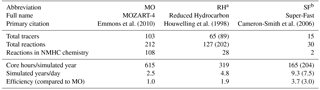
a Unmodified RH listed in the parentheses. b SF + Bulk Aerosol Model (BAM) included in parentheses.
2.2.1 MOZART-4
The MOZART-4 mechanism (Emmons et al., 2010; Lamarque et al., 2012; Tilmes et al., 2015) is the standard tropospheric chemical mechanism used within the CESM CAM-chem framework (Tilmes et al., 2015, 2016). It has been used in many model intercomparison projects (e.g., Lamarque et al., 2013; Emmons et al., 2015) and extended to tagged tracer chemistry (Emmons et al., 2012). As described in detail in Emmons et al. (2010), the MOZART-4 mechanism is a tropospheric mechanism that contains 85 gas-phase species and 12 bulk aerosol species, with 39 photolysis and 157 gas-phase reactions. Large alkanes, alkene, and aromatics are lumped together (BIGALK, BIGENE, and TOLUENE, respectively), and monoterpenes are lumped together as C10H16 and treated as α-pinene. We use the FMOZSOA compset (see http://www.cesm.ucar.edu/models/cesm1.2/cesm/doc/modelnl/compsets.html, last access: 10 October 2018) and make modifications to the chemical mechanism input files (see “Code availability” section) and emission files for the following mechanisms.
2.2.2 Reduced hydrocarbon
The RH chemical mechanism (Houweling et al., 1998; Lamarque et al., 2010) is a reduced-form mechanism based on the Carbon Bond Mechanism 4 (CBM-4) (Gery et al., 1989). The CBM-4 was developed to simulate polluted regional chemistry, and the RH mechanism updated and expanded this mechanism to also be capable of simulating background low-NOx conditions (Houweling et al., 1998). As described in Houweling et al. (1998), the original RH mechanism has 30 tracers and 68 total reactions. It has been used extensively in model intercomparisons (e.g., Pöschl et al., 2000) and is generally considered a satisfactory reduced hydrocarbon mechanism (e.g., Hauglustaine et al., 1998; Wang and Prinn, 1999; Granier et al., 2000; Pfister et al., 2014). Lamarque et al. (2008) incorporated the RH mechanism into the CESM CAM-chem framework with a few updates, and Lamarque et al. (2010) expanded it to 89 (to include the bulk aerosol model species) tracers and 202 total reactions. As the lumping of alkanes and alkenes in RH differs from the MO mechanism, a mapping between the differently aggregated species is necessary (see Table S1).
For this work, we modified the RH mechanism to remove many of the tracers and reactions that are pertinent primarily to stratospheric chemistry (as introduced in Lamarque et al., 2008) since these simulations include specified long-lived stratospheric species (O3, NOx, HNO3, N2O, N2O5) as in MOZART-4 (Emmons et al., 2010). However, the unmodified RH mechanism can be run with the more complex stratospheric chemistry but at a significant additional cost. This is not considered in this paper to allow a better comparison between the tropospheric-only mechanisms. The modified RH mechanism, which shows only minor differences in the simulated surface ozone concentration from the complete mechanism (not shown), contains 65 tracers and 127 reactions. This RH mechanism runs approximately twice as fast as the MO mechanism under our current configuration (Table 1).
2.2.3 Super-Fast
The SF mechanism is a highly simplified chemical mechanism designed to efficiently simulate background tropospheric ozone chemistry (Cameron-Smith et al., 2006, and the Supplement of Lamarque et al., 2013) and has been included in many model intercomparison projects, including ACCMIP (Lamarque et al., 2013). These intercomparisons included studies which examined the following: historical simulations to simulations to the end of the 21st century (1850–2100) (Young et al., 2013), historical tropospheric O3 changes and radiative forcing (Stephenson et al., 2013), and CH4 and OH lifetimes under present-day and future conditions (Voulgarakis et al., 2013). Generally, the SF mechanism falls within the range of ACCMIP results, with some exceptions that we briefly describe here and in more detail in the Supplement. In general, the SF mechanism has performed reasonably well for those species included in the mechanism.
The SF mechanism only simulates sulfate aerosol, so comparisons with the aerosol simulations of the other ACCMIP members were not possible (Lamarque et al., 2013). The SF simulations within ACCMIP demonstrated lower rates of ozone chemistry and deposition resulting in a low ozone burden bias (−10 %) and a high ozone lifetime bias (+14 %) (Young et al., 2013); however, historical and projected changes in ozone tropospheric column and radiative forcing fell within the ACCMIP range (Stevenson et al., 2013). Human health analysis with the SF simulations fell within the range of the other ACCMIP members (Silva et al., 2013, 2016, 2017). Squire et al. (2015) compared SF to more complicated isoprene schemes and concluded that including the SF mechanisms is preferable to neglecting chemistry entirely, although there are biases in regions of high biogenic chemistry. Schnell et al. (2015) conclude that the SF mechanism responds differently than other more complex mechanisms, particular under different Ox production regimes (e.g., SF shows a net increase in Ox production when isoprene emissions increase in NOx-limited regions, whereas the other mechanisms show a net decrease or little change). Finally, Schnell et al. (2015) compare seasonal and diurnal cycles to other mechanisms, and the SF mechanism simulates high ozone events in the springtime, and they find that the SF mechanism outperforms others mechanisms when compared to the observed summertime diurnal cycle. An extended review of the SF mechanism performance within model intercomparisons can be found in the Supplement.
The SF mechanism includes 15 chemical tracers with 6 photolysis reactions and 24 gas-phase reactions, making it the simplest chemical mechanism to be included as a member of the ACCMIP ensembles (Lamarque et al., 2013). It was developed by the Lawrence Livermore National Laboratory (LLNL) and has not been described as implemented within the CESM code, so we include a description here and in our Supplement. Table S2 summarizes the SF mechanism photolysis and gas-phase reactions, which consist of a basic methane oxidation scheme (CH4, CH3O2, CH3OOH, CH2O, and CO), with basic oxidant chemistry (OH and O3), along with simple sulfur chemistry (dimethyl sulfide (DMS), SO2, and SO4) and a single biogenic hydrocarbon species, isoprene (ISOP), with two oxidant pathways: ISOP + OH and ISOP + O3. For Reactions (iii), (vi), (10), (11), and (15) (Table S2), it is assumed that their products O, H, and CH3OH are instantaneously converted to their ultimate products O3, HO2, and HO2, respectively. Nitric acid chemistry is limited to two reactions, one of which requires a heterogeneous reaction parameterization. Sulfur chemistry is limited to four reactions. Isoprene chemistry is highly parameterized. The reaction of isoprene with OH is based on the net effect of the reaction in the University of California Irvine (UCI) model (Wild and Prather, 2000), namely ISOP . This particular parameterized reaction, which when originally implemented used a negative coefficient among the products (ISOP ), is not standard within the CESM chemical modeling framework and cannot be handled by the solver, so the equivalent triple reaction formulation of (21a), (21b), and (21c) is required. The oxidation of isoprene by ozone is a simple parameterization (resulting in the fractional production of only the species that already exist in the mechanism as part of the methane oxidation scheme: CH2O, CH3O2, HO2, and CO) derived from the net effect of the isoprene or ozone oxidation pathways from the full LLNL-IMPACT model (Rotman et al., 2004) and was included specifically to improve the simulation of surface ozone chemistry (Cameron-Smith et al., 2009). We map the MO isoprene directly to the single SF isoprene species (ISOP).
Much of the simplicity within the SF mechanism comes from what it does not include. Carbon chemistry is limited to the five single-carbon species used in the simple methane oxidation scheme, plus isoprene. There is no PAN (peroxy acetyl nitrate) or ammonia, and hence no nitrogen aerosols, although HNO3 is created in Reactions (8) and (16). These all impact ozone chemistry, but the inclusion of additional hydrocarbon, aerosol, or heterogeneous chemistry would introduce significant additional computational costs (similar to the more complete mechanisms). There are no halogen species, since this would require the inclusion of a significant number of additional chemical tracers, and as such there is no capability to describe the polar ozone hole phenomenon within the mechanism (Cameron-Smith et al., 2006), so it is implemented within Linoz using the simple loss parameterization of Cariolle et al. (1990). The greatest simplifications in the SF mechanism arise from compacting all of the non-methane hydrocarbon chemistry (NMHC) into two isoprene reactions, and thus there is none of the complex chemistry that is required to adequately represent ozone chemistry in highly polluted regions. The simplicity of the SF mechanism allowed us to perform three short simulations in which we added reduced-form PAN and N2O5 chemistry (individually and in conjunction) from the MOZART-4 mechanism into the SF mechanism, which we use as a demonstration of the type of sensitivity tests that are possible with the SF mechanism. This type of quick sensitivity test would be significantly more difficult with the more complex mechanisms, given the complexity of PAN and N2O5 chemistry.
2.3 Computational requirements
The computational requirements of MO, RH, and SF as simulated on the NCAR Cheyenne supercomputer are summarized in Table 1. The computational cost results from both the chemical solver and the advection of the chemical tracers within CAM-chem. No load balancing was conducted, which could potentially increase the efficiency of the RH and SF mechanisms. The CESM1.2 CAM-chem model run with the SF mechanism is roughly 3 times faster than a run with the MO mechanism when the Bulk Aerosol Model (BAM) (see Tilmes et al., 2015) aerosols are included (which we do not examine in this present study), and a gas-phase-only simulation with the SF mechanisms increases the speeds to nearly 4 times as fast. The RH mechanism is roughly twice as fast as the MO mechanism. At higher spatial resolutions, the computational advantage of the SF mechanism over the more complex MO and RH schemes is likely to increase, since advection of tracers typically becomes a larger fraction of the total model run time.
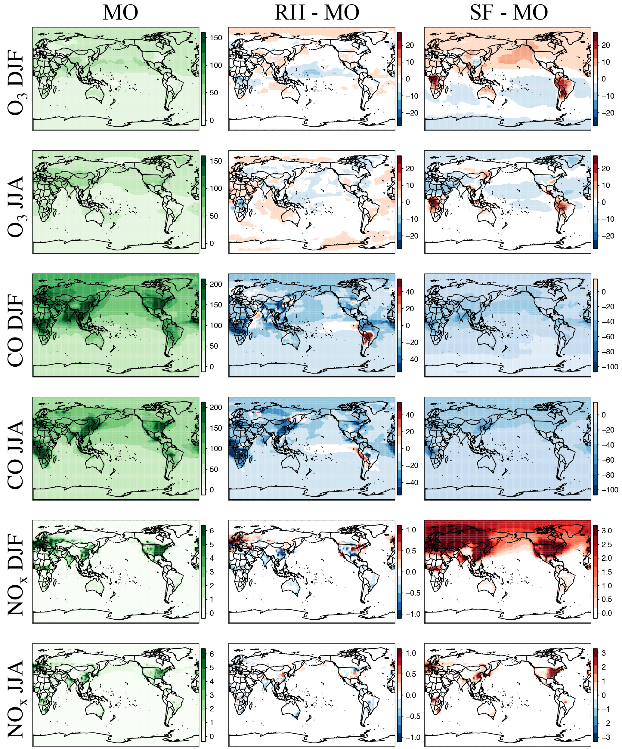
Figure 1Maps of DJF and JJA O3, CO, and NOx for MO, the difference between RH and MO, and that between SF and MO for the year 2015. The chemical units are in ppb. Please note the difference in the chemical scales for each panel. Cool colors for the difference panels indicate MO is higher, and warm colors indicate that RH or SF is higher.
2.4 Observations
The ozone observational databases are of two types: the global database is ozonesonde data compiled from Tilmes et al. (2012) while the US database comes from the EPA Clean Air Status and Trends Network (CASTNET), which has more than 90 surface observational sites within the United States and has been collecting surface meteorological and chemical data since 1990 (CASTNET, 2016, and https://www.epa.gov/castnet). We used data from all sites that reported complete ozone data from each year, after removing data that the CASTNET database marked as invalid. The number of sites that matched these criteria varied from year to year, but generally we have between 55 and 94 sites throughout the 1991–2015 period. The CASTNET observational network is located primarily in rural sites and thus is a reasonable comparison to coarse-grid cell model output (e.g., Brown-Steiner et al., 2015, and Phalitnonkiat et al., 2016). In order to compare to the CESM CAM-chem simulations, which have no emissions trend, we have detrended the CASTNET data for each region using a simple linear regression. Regional averaging is first done by averaging all observational sites within a single grid cell and then averaging to the larger regions as needed. We also compare to ozone precursor species observations from Tilmes et al. (2015).
3.1 Spatial comparisons
The spatial distribution of ozone and related species between the three mechanisms are compared in Fig. 1. Taylor-like diagrams comparing results to ozonesondes over different global regions are provided in Fig. 2 and comparisons to aircraft observations in Fig. 3. Globally averaged surface daily maximum 8 h (MDA8) O3 is consistent across all mechanisms (Table 2) with the largest spatial differences (especially with the SF mechanism) noted over regions of intense biomass burning or biogenic emissions, such as equatorial Africa and South America, as well as over Northern Hemisphere oceans within SF (Fig. 1). Surface CO mixing ratios show small regional differences between MO and RH, while NOx mixing ratios show very small and highly localized differences (Fig. 1). All three mechanisms tend to have low CO biases over much of the Northern Hemisphere, with SF showing the largest bias. This coincides with starkly higher NOx mixing ratios in the Northern Hemisphere (Figs. 1, 3), especially in the winter and spring seasons. This is explored in more detail below.
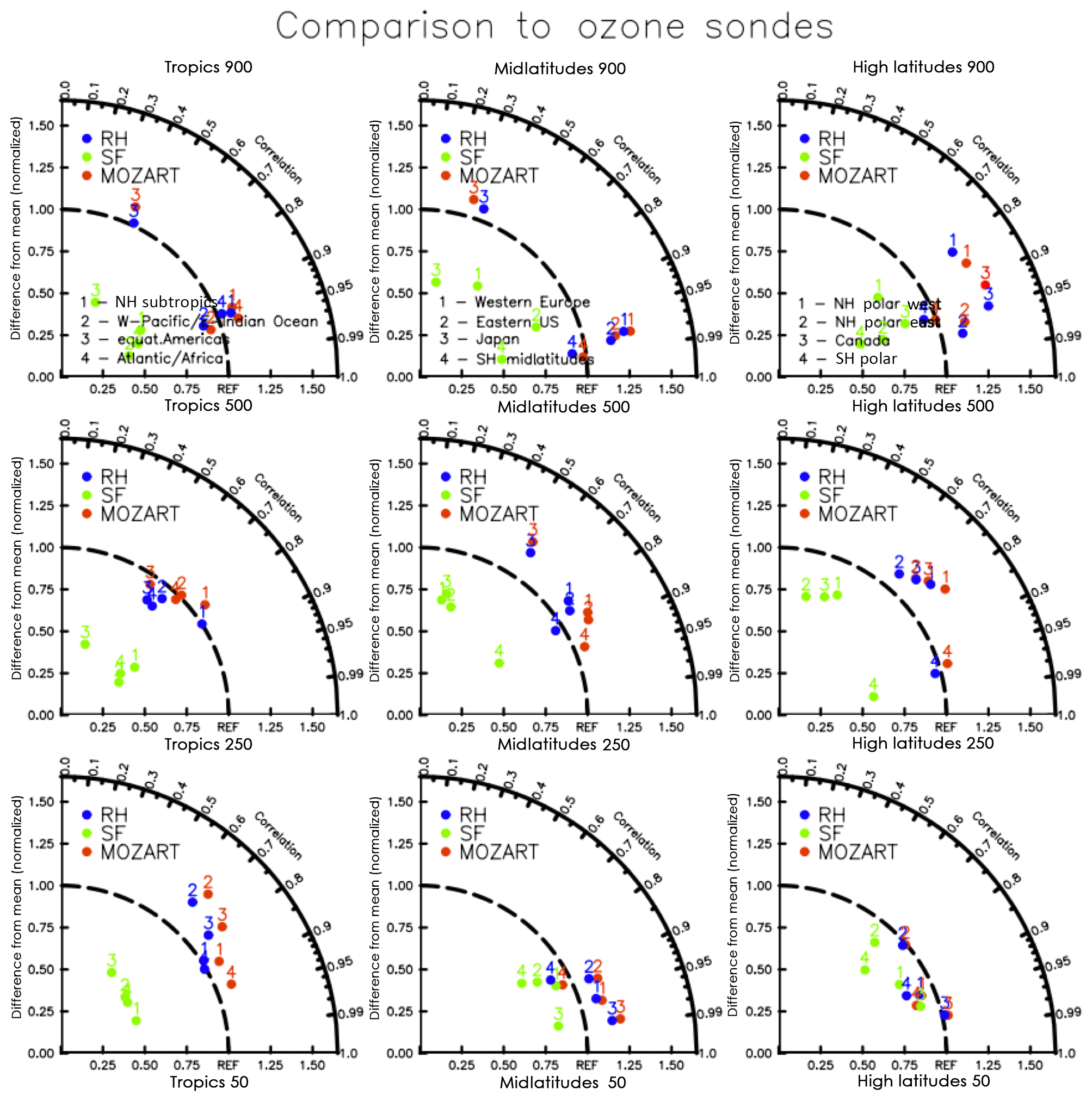
Figure 2Taylor-like diagrams comparing the mean and correlation of the seasonal cycle between observations (present-day ozonesonde climatology – Tilmes et al., 2012 – from 1995 to 2011 for different regions (tropics, midlatitudes, and high latitudes) and different pressure levels (900, 250, and 50 hPa), as in Fig. 12 of Tilmes et al., 2015, and simulations (red: MO; blue: RH; green: SF).
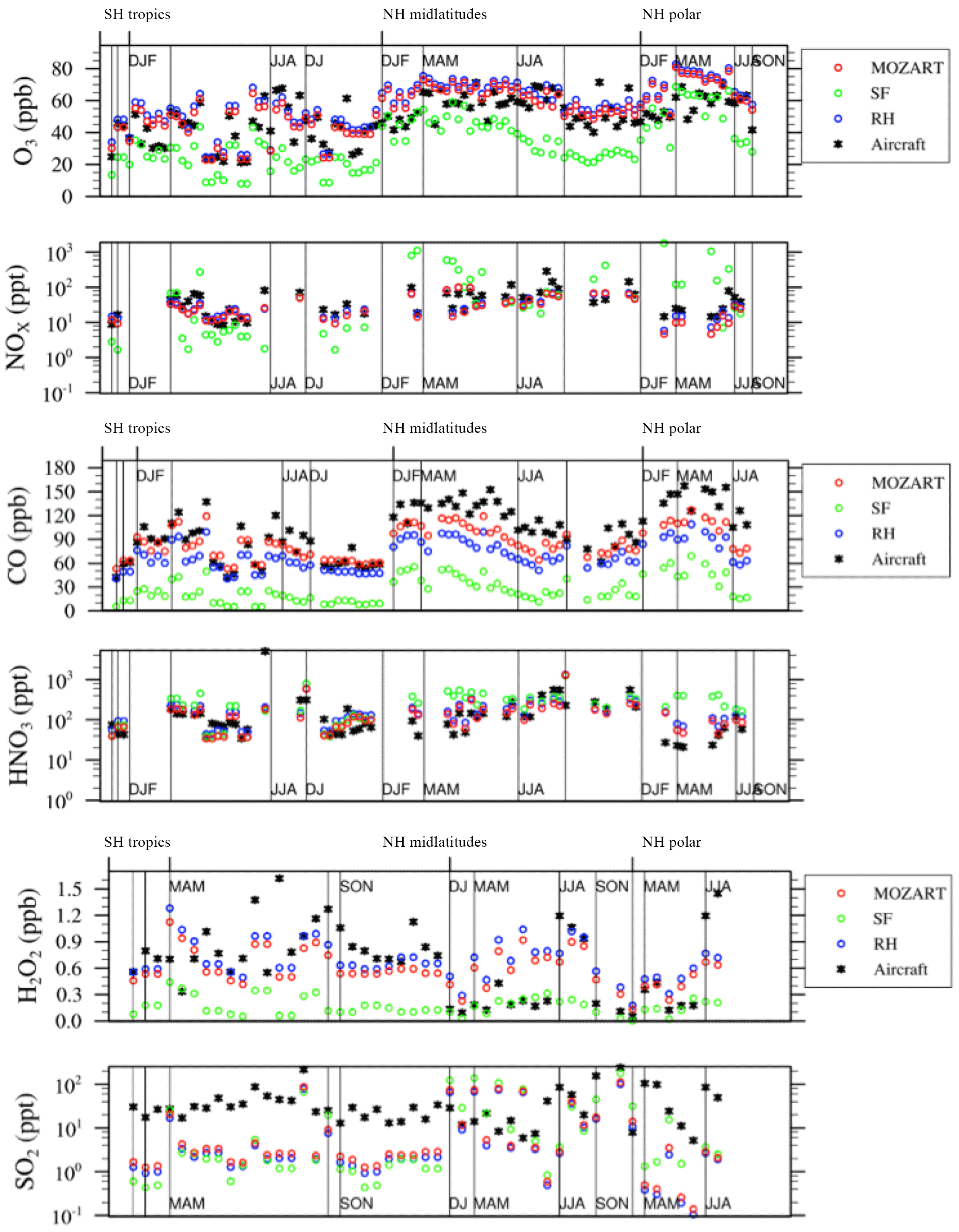
Figure 3Relative differences between available aircraft observations (black) and the MO, RH, and SF model configurations (colors) over different regions and seasons, averaged over 2–7 km, for O3, NOx, CO, HNO3, H2O2, and SO2 as in Fig. 17 of Tilmes et al. (2015).
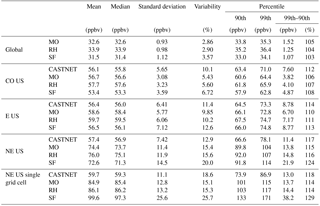
Table 2Summary statistics for the daily maximum 8 h (MDA8) O3 over the globe and over the indicated regions in the US. Additional regions can be found in Table S3.
Zonal profiles (Fig. 4) show that ozone is similar among all mechanisms for all seasons, especially in the lower troposphere. Compared to the MO mechanism, the SF mechanism simulates higher Northern Hemisphere ozone in the winter, and lower in the summer. Both the RH and SF mechanisms simulate lower CO mixing ratios than the MO mechanism in both the summer and winter, with the SF mechanism diverging the most in the Northern Hemisphere in the summer. The SF mechanism also simulates higher NOx in the Northern Hemisphere winter, which (as we explore below) may in part be due to the lack of PAN chemistry.
At the largest spatial scales, all three mechanisms predict similar levels of surface ozone (Fig. 5, Table 2), with global surface ozone estimates of 32.6±0.93, 33.9±0.98, and 31.5±1.12 ppb for MO, RH, and SF, respectively. Even at the continental-US scale, all three mechanisms estimate similar surface MDA8 O3 values (56.7±3.08, 57.7±3.23, and 53.4±3.59 ppb for MO, RH, and SF, respectively), which are consistent with the CASTNET observations of 56.1±5.65 ppb. However, within the northeastern US, the well-known high bias is apparent (74.4±11.4, 76.0±11.9, 72.6±14.5 ppb for MO, RH, and SF, respectively, while the CASTNET observations are 57.4±7.42 ppb). The MO and RH mechanisms are nearly identical at all spatial scales, while the SF mechanism simulates larger MDA8 O3 variability, especially at individual grid cells within the eastern US. Taking into account the model ozone biases, the SF is a better characterization of the ozone distribution (as compared to CASTNET) for almost every spatial scale examined within the US. Indeed, in the southeastern US, where we expect SF to perform poorly due to the simplified biogenic species chemistry, we actually find that the SF estimates the shape of the high ozone tail better than either MO or RH: CASTNET estimates at an individual grid cell that the 99th percentile for MDA8 O3 is 18 % higher than the 90th percentile (Table 2), and while MO and RH both estimate it to be only 14 % higher, the SF estimates it to be 29 % higher. In Sect. 4, we explore some of the implications of these differences and in particular whether the biases within the SF mechanism are of the same magnitude as some of the biases within the MO and RH.
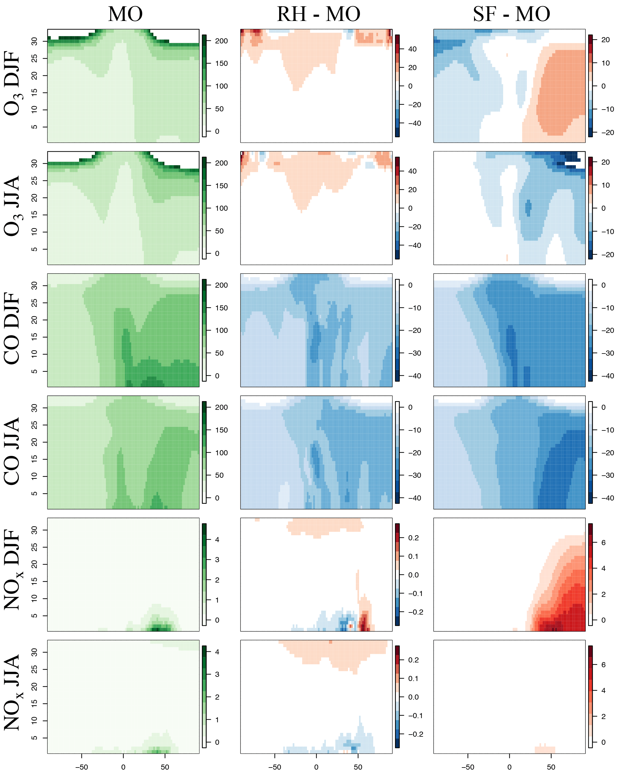
Figure 4Zonal plots of seasonal O3, CO, and NOx for MO, the difference between RH and MO, and between SF and MO for the year 2015. The vertical axis is the model level, and the chemical units are in ppb. Please note the different vertical axis in each row. Cool colors for the different panels indicate MO is higher, and warm colors indicate that RH or SF is higher.

Figure 5Surface JJA MDA8 O3 boxplots for the 1991–2014 data for CASTNET (grey), MO (red), RH (blue), and SF (green) averaged over the various regions. Plots (g, h, i) are individual grid cells from within each region (38.8∘ N and 87.5∘ W for g, 38.8∘ N and 80.0∘ W for h, and 33.2∘ N and 85.0∘ W for i). Global boxplots are included along with the continental US. The units are in ppb, and for each boxplot the box contains the interquartile range (IQR), the horizontal line within the box is the median, and the whiskers extend out to the farthest point which is within 1.5 times the IQR, with circles indicating any outliers. Note the scale difference between the top row and the rest of the panels.
Figure 6 explores this finding, which plots the percentage difference between the 99th and the 90th percentile ozone as the length of the time series included grows. This comparison allows for a comparison of the relative distribution among mechanisms, here for the higher end of ozone values, to compare the overall shape of each mechanism's distribution when biases in the magnitudes are normalized. We note that (1) it takes between 5 and 10 years before a consistent and stable estimate emerges with each simulation, indicating that simulations less than 10 years may be inadequate for comparisons between chemical mechanisms; (2) the CASTNET observations have a transient estimate, most notably in the southeastern US, which indicates a divergence of the 99th and the 90th percentiles (i.e., a lengthening of the upper tail) that is not seen in the simulations; and (3) the SF mechanism is inconsistent with the MO and RH mechanisms, which are nearly identical, but the SF mechanism estimate is also closer to the CASTNET estimate in the midwestern and southeastern US. Whether this is the result of fortunate biases within the SF mechanism or an implication that the more complex chemistry within the MO and RH mechanisms are underestimating the length of the ozone tail requires further study. Brown-Steiner et al. (2018a) examines these implications, and also concludes that it takes approximately 10 years for long-term signals to emerge from meteorological variability. These results demonstrate the challenge in examining chemical signals in highly variable data, particularly if there are trends or changes to the ozone distribution, as is seen in the CASTNET data for the southeastern US.
However, while the SF mechanism performs as well as, or better than, the MO and RH mechanisms in certain regions, there are many regions – especially in the northernmost latitudes over land and over equatorial land masses – where the SF mechanism is far less capable at simulating surface ozone than either the MO or RH mechanisms. Figure 7 plots R2 values for the MDA8 O3 JJA time series (1990–2015) at every grid cell between the MO mechanism and both RH and SF, and it is clear that the RH mechanism has very high R2 values (R2>0.75) over much of the globe. And while the SF mechanism has large R2 values over many regions – in particular the extratropics – over the equatorial regions, and especially over land, R2 values drop below 0.5 and even 0.25.

Figure 6The relative difference (%) between the 99th percentile and the 90th percentile of JJA MDA8 O3 for CASTNET and the three mechanisms over three regions as a function of increasing length of simulation, from 1 day up to the full 25 years simulated. The vertical bars indicate the year 2000, for which the emissions for all three simulations were cycled.
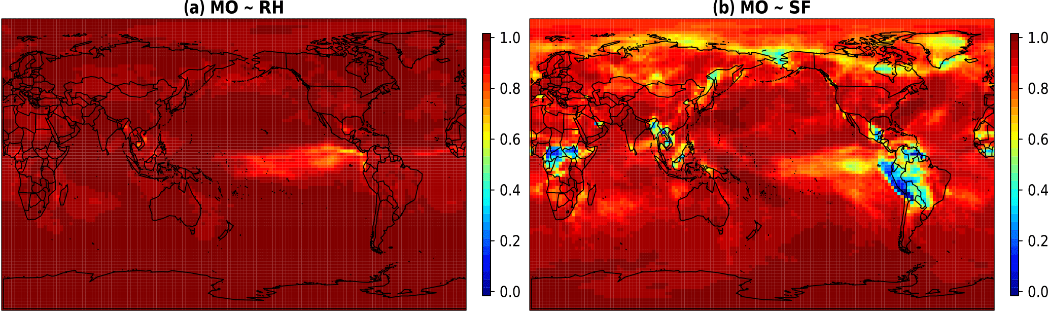
Figure 7R2 values calculated at every grid cell (for the full 1991–2015 MDA8 O3 JJA time series) for MO and RH (a) and MO and SF (b).
3.2 Seasonal and diurnal comparisons
The seasonality of surface ozone is similar among all three mechanisms at the regional scales (Fig. 8), although differences occur at both the largest and smallest scales: (1) the SF mechanism simulates a dual-peaked maximum in surface ozone averaged at the global scale, a phenomenon also noted by Schnell et al. (2015); (2) this dual-peaked maximum is still apparent at the regional scales, although to a much lesser degree; and (3) the RH mechanism has a dual-peaked maximum over portions of the southeastern US. The seasonal patterns for CO and NOx are consistent across all models, although CO is lower in both RH and SF than in MO for all seasons. RH and MO NOx levels are nearly identical, but SF simulates higher values for NOx in all seasons, and particularly in the winter and spring seasons, as already noted. HOx and isoprene seasonality is consistent across all mechanisms at most scales. Diurnal cycles are compared for a single grid cell within the central US in Fig. 9. With the exception of isoprene within the SF mechanism, which does not adequately represent nighttime isoprene chemistry, the diurnal cycles are comparable across all mechanisms for most species. The MO and RH mechanisms are nearly identical, with the exception of CO values, as already mentioned. The SF mechanism tends to show more extreme peaks in OH and NOx and lower levels of O3, CO, H2O2, and (Fig. 9). Surface levels of O3 and CO within the SF mechanisms are sensitive to the addition of PAN and N2O5 chemistry (the dotted lines in Fig. 9), described below, although the sensitivity tends to be in the simulated magnitude and not the shape of the diurnal cycle.
Figures 8 and 9 also include 2-year simulations (1990–1991, with year 2000 emissions) which we included in the SF mechanism PAN and N2O5 chemistry taken (and reduced) from the MOZART-4 mechanism. We examine these mainly to demonstrate the potential for the modification of the SF mechanism to meet particular research needs. Largely, the addition of PAN chemistry (purple lines) results in more substantial changes to various species than the addition of N2O5 chemistry (orange lines), but their combined addition (green lines) slightly modifies the simulated large-scale values of O3, CO, HOx, and isoprene. The addition of PAN chemistry brings the SF mechanism simulations closer to the MO mechanism for the NOx and HOx seasonal cycles (Fig. 8) and the CO diurnal cycle (Fig. 9) but at the expense of the global-scale capability to simulate ozone and isoprene. Additional tuning of the parameterized Reactions (21) and (22) (Table S2) may be able to correct these errors. Sulfate aerosol in the SF mechanisms is notably lower than in both the MO and RH mechanisms, which may result from the simple aerosol scheme within the SF mechanism.
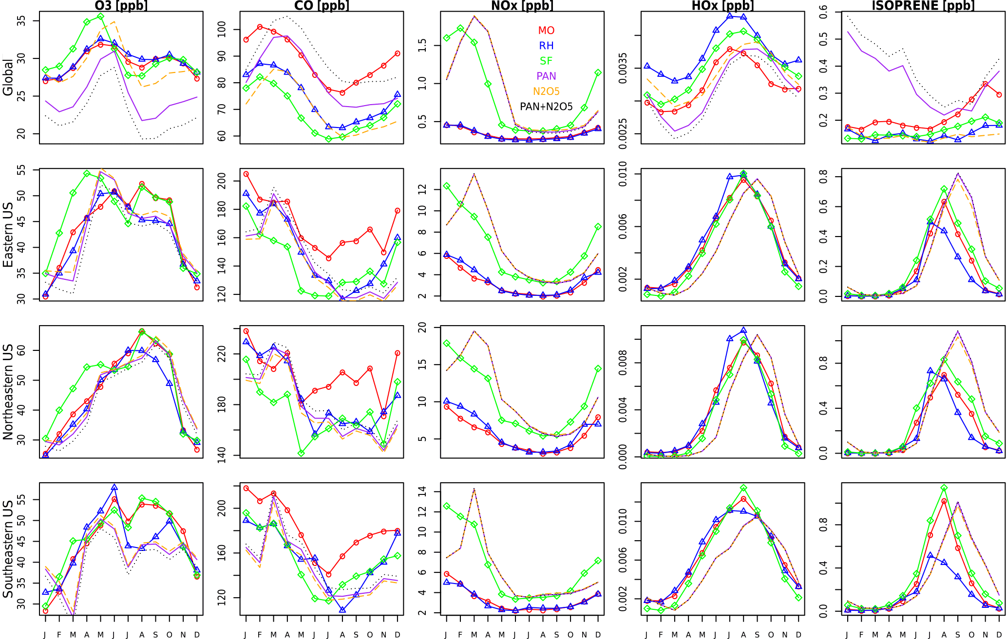
Figure 8Seasonal time series for O3, CO, NOx, HOx, and ISOP for MO (red), RH (blue), and SF (green) for a single year (2015), averaged over different regions. The units are in ppb. Note the different scales in each panel. Also included are three sensitivity tests conducted with the SF mechanism (which were run for only 2 years, 1990–1991, with 1991 being plotted here): adding PAN chemistry (purple), adding N2O5 chemistry (orange), and adding both PAN and N2O5 chemistry (black).

Figure 9Example diurnal time series for various species for MO (red circles), RH (blue triangles), and SF (green diamonds) averaged over a single grid cell in the central US (100∘ west and 47∘ north). The units are in ppb. Also included are three sensitivity tests conducted with the SF mechanism: adding PAN chemistry (purple), adding N2O5 chemistry (orange), and adding both PAN and N2O5 chemistry (black).
3.3 Comparison to observations
Figure 10 compares the model estimates of surface ozone to observations (ozonesondes and CASTNET observations) for different spatial regions, as well as to each other. Generally, all three mechanisms simulate less variability over continental to global-scale regions than the ozonesonde observations (Fig. 10c–e) and show a high bias over many sites within North America, Europe, and Asia. Within the US, all mechanisms show a high bias in the eastern US, and especially in the northeastern US, but the variability is well-captured when compared to CASTNET (with slopes ranging from 0.61 to 1.24 in Fig. 10f–h). When compared to each other (Fig. 10a, b, i, j), the RH mechanism and MO mechanism are nearly identical. The SF mechanism, while comparable to the MO mechanism at many sites, shows greater divergence, overestimating values in many grid cells throughout the globe (Fig. 10b) and both over- and underestimating within the US (Fig. 10j). Taylor-like diagrams are plotted in Fig. 2 and show the close clustering of the MO and RH mechanisms and that the SF mechanism differs from the observations at a similar magnitude to the MO and RH mechanism for some regions but performs poorly in other regions (especially in the tropics, where tropospheric ozone is underestimated with the SF mechanism).
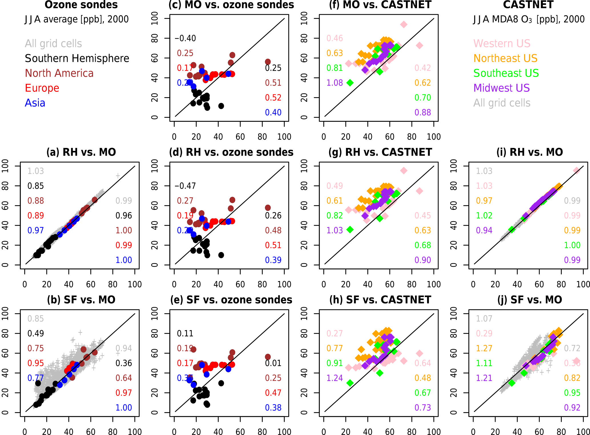
Figure 10Scatterplots comparing model results to observations (two center columns) and to each other (two outer columns). Global comparisons to observations (c, d, e) compare model results to ozonesondes (JJA averages), while regional comparisons to observations (f, g, h) compare the model results to CASTNET surface observations (JJA MDA8 O3). For the model-to-model comparisons (global in a, b and within the US in i, j), grey symbols additionally compare every grid cell in the model output. The numbers within each subplot indicate the slope (left hand side) and R2 values (right hand side) for each region. Each panel is labeled with the following convention: “y axis” vs. “x axis”.
Our primary objective has been to determine what is lost (or gained) with the selection of a simplified chemical mechanism, which we summarize here. We mostly discuss the SF mechanism, as the trade-offs with the RH mechanisms are straightforward: we lose very little (Fig. 10a and i) and gain about a 100 % increase in simulation speed (Table 1). Many of the things that are lost with the use of the SF mechanism are expected: we lose the capability to directly simulate small-scale features of ozone chemistry in regions that depend strongly on complex biogenic chemistry. In particular, the equatorial landmasses – especially equatorial Africa and South America – are not well simulated (Fig. 7). We also lose the capability to simulate some of the short-term features that require additional chemistry, such as the nighttime behavior of isoprene (Fig. 9) or the cold season CO and NOx behavior (Figs. 1 and 4). The addition of PAN and N2O5 chemistry does not rectify the nighttime behavior of isoprene (Fig. 9) but do bring the cold-season-simulated CO and NOx mixing ratios closer to the MO mechanism (Fig. 8). These deficiencies may result from the highly parameterized biogenic chemistry within the SF mechanisms (Table S2), although it may also result from the treatment of isoprene emissions, and future simulations will need to consider the trade-off between additional complexity and computational efficiency.
More surprisingly, there are several desirable capabilities that are not lost with the selection of the SF mechanism. For most regions, the selection of the SF mechanism does not degrade the estimate of surface ozone (both the magnitude and the variability), nor do we lose features of the daily variability that results from the meteorology. In many regions, and at many scales, we find that the selection of the SF mechanism introduces uncertainties that are smaller than the difference between the simulated and observed surface ozone mixing ratios (Fig. 5). Surface layer ozone is adequately represented over many regions in all seasons within the SF mechanism (Fig. 8), despite the high CO and low NOx levels in the winter and spring seasons (Fig. 4). For these seasons, the adequate ozone representation may be the result of compensating errors, and Schnell et al. (2015) previously found comparable cases where the SF mechanism outperforms more complex models, perhaps due to various sets of compensating biases or errors.
We now turn to the main question of this research: what do we gain when we select a simplified chemical mechanism? The primary thing we gain is the capability to simulate longer periods of time or to include more members in an ensemble in proportion to the simplicity of the mechanism. Our results show that, without any optimization of the code, the RH mechanism is ∼100 % faster than the MO mechanism, and the SF mechanism is up to 200 % faster than the MO mechanism (Table 1). We feel that the capability to run three SF simulations for the price of one MO simulation under different sets of initial conditions, for example, can extend the quantification of parametric uncertainties, which is largely unavailable to the most complex and most computationally demanding mechanisms. Of course, the SF mechanism may not be appropriate for every sensitivity study but neither is the MO mechanism. The choice of mechanism really depends, then, on the science question. If the research objective is to predict complex chemistry–climate interactions and if computational resources are available, then a more complex mechanism will have the most value. However, if the research objective is to better understand various parameterizations, then a more computationally efficient mechanism will have higher value even if it might not be capable of accurately simulating all variables in detail (Hoffman et al., 1996). This is particularly the case when a baseline can be established between the simplified mechanism and the complex mechanism, as we have done here. We feel that this parallel approach, in which a set of mechanisms with varying levels of complexity are run concurrently with a consistent set of parameters, allows us to enhance our exploration of uncertainties and thus our ability to understand the atmospheric chemistry of the Earth system.
For instance, there are many research frameworks where the “three-for-one” advantage of the SF mechanism could be utilized with the MO mechanism, in which one simulation of a 5- or 10-year time slice with the MO mechanisms could be combined with three simulations of the SF mechanism, one matching the parameters of the MO mechanism (in order to provide a consistent baseline) and the other two exploring other parameter spaces (e.g., different initial conditions or different emission scenarios). The establishment of a baseline comparison is particularly important, since the SF mechanism is a simplified mechanism and should not be blindly trusted to reproduce the behavior of more complex mechanisms. For example, if a research group is interested in precise estimates of ozone concentrations in regions where the biogenic influence is significant, the SF mechanism would prove insufficient. The RH mechanism may be sufficient, but the more modest increase in computational speed – a “two-for-one” advantage over the MO mechanism – may not be enough to justify the simulation. If, however, the phenomenon of interest can be shown to be within the SF mechanism capabilities (e.g., simulating regional-scale ozone, as shown in this paper), the “three-for-one” advantage of the SF mechanism is readily apparent. The SF mechanism may be particularly desirable with chemistry–climate simulations at higher spatial resolutions.
In addition, the selection of a simplified mechanism allows for the capability to easily and efficiently test new forms and new representations of chemistry without the need to painstakingly update and test all possible interactions of any addition within a complex mechanism. For example, in this study, we added a simplified PAN and N2O5 representation to the SF mechanism (Figs. 8 and 9) to see how it improves the simulations. This exercise offered a significant capability to test, simulate, and further learn about improving atmospheric chemistry computations. This demonstrates that a hybrid approach (or tiered approach, as recommended in Uusitalo et al., 2015) – in which complex and trusted chemical mechanisms are used to evaluate simplified mechanisms that can run for longer periods or with increased ensemble members – has the potential to maximize computational capabilities and to get the most out of atmospheric chemistry modeling.
Furthermore, the selection of a simple chemical mechanism – especially when used in conjunction with more complex mechanisms within a consistent modeling framework – allows for better quantification of the uncertainties and the relative importance of particular pieces of the chemistry. Here, for instance, the SF mechanism's representation of biogenic species chemistry is insufficient to adequately represent equatorial landmasses, but the reduced-form RH mechanism is nearly as capable as the MO mechanism over most regions and most species. This begs the following question: is there a representation of biogenic chemistry somewhere between the RH and the SF mechanisms that can approach the efficiency of the SF mechanism and the accuracy of the RH mechanism? We hope that future research will address this question, as well as others, such as more globally oriented research pertaining to ozone budgets and the interaction between OH and CH4 lifetime. In addition, comparisons of chemical mechanisms of different complexities, particularly where the simplified mechanisms fail, could potentially identify regional chemical regimes. For instance, the SF mechanism cannot adequately represent the chemistry of equatorial forests (Fig. 7), and the spatial regions that fail to simulate ozone chemistry are similar to the spatial distribution of the tropical forest chemical regime identified in Fig. 4 of Sofen et al. (2016), which utilized a statistical clustering technique to identify chemical regimes. Finally, the capability to examine atmospheric chemistry complexity in a step-wise fashion could also be utilized to bridge the gap between the most complex 3-D chemical models and the more efficient models utilized by the Earth models of intermediate complexity (EMIC) or integrated assessment model (IAM) communities.
In this study, we have compared three chemical mechanisms of different levels of complexity within the CESM CAM-chem framework for present-day chemical and climatological conditions. We conducted 25-year cycled emission simulations nudged to MERRA meteorology with the standard tropospheric MOZART-4 (MO) mechanism of Emmons et al. (2010), the Reduced Hydrocarbon (RH) mechanism of Houweling et al. (1998), and the Super-Fast (SF) mechanism of Cameron-Smith et al. (2006). The RH mechanism is roughly twice as efficient as the MO mechanism, and the SF mechanism is roughly 3 times as efficient as the MO mechanism, without any code optimization. As much as possible, we kept the parameterizations consistent across all mechanisms, although we had to remap some of the MO mechanism species to match up with the RH mechanism species.
We examine present-day chemistry with MO, RH, and SF. Both MO and SF have been compared in other model intercomparisons, including for preindustrial conditions (see the Supplement for additional information). We hope that the analysis presented in this paper and the availability of the mechanism files (Supplement) will provide a baseline for continuing research on both the RH and SF mechanisms.
We find that all three mechanisms successfully capture surface ozone values at the larger spatial scales, but at smaller spatial scales, and especially within the northeastern US, all three mechanisms have surface ozone biases when compared to CASTNET observations; however, the mean values for all three mechanisms are consistent with each other at a variety of spatial scales. The SF mechanism simulations show larger ozone variability than the MO and RH simulations, although when normalizing the distributions to account for the known ozone biases, the SF mechanism represents the shape and spread of the ozone distributions better than the MO or RH mechanisms when compared to the CASTNET observations (Fig. 5).
The RH mechanism is in close agreement with the MO mechanism for nearly every metric we examined, and any differences tend to be minor (both in magnitude and in spatial extent). The SF mechanism simulates higher NOx and lower CO than the MO mechanism, and the NOx deviations are particularly large in the winter season. In addition, the SF mechanism deviates from the MO mechanism over regions of high biogenic emissions, such as equatorial Africa and South America. These large deviations within the SF mechanism are likely a result of the simplicity of the mechanism and especially of the lack of biogenic species chemistry beyond a single-species, two-reaction representation as well as a lack of PAN and N2O5 chemistry (Figs. 8 and 9). The SF mechanisms do not include NO3, which may also explain some of the nighttime biases. Future simulations in which NO3 chemistry is added to the SF mechanism may correct some of these biases. We also find that although the SF mechanism differs in the magnitude of the estimated ozone from the other two mechanisms, the simulated ozone variability is similar in all three mechanisms (Figs. 4 and 10).
We find that there are significant gains that can be realized by a research approach that utilizes simulations with both a complex and a simplified chemical mechanism where the complex mechanisms are used to provide a more trusted chemical result (especially for the mean values) and the simple mechanism could be used to efficiently simulate longer time periods to better understand the roles of meteorological variability. The capability of the SF mechanism to simulate adequate chemistry with interactive meteorology is not examined here nor is the coupling of the SF mechanism with modal aerosols, which is left for future research. These results encourage revitalizing or creating simplified chemical mechanisms within individual modeling frameworks and examining the structural uncertainties that exist between different models with regards to simplified chemical mechanisms.
Finally, we note that there are many inherent uncertainties associated with the use and comparison of chemical mechanisms and climate–chemistry simulations, many of which are inherited with the adoption of a particular model. The CESM CAM-chem model has been used extensively to examine a variety of climate and chemistry phenomena, and uncertainties that arise from the individual choices made during the historical development of this chemical model (see Brasseur et al., 1998; Hauglustaine et al., 1998; Horowitz et al., 2003; Kinnison et al., 2007; Emmons et al., 2010) are still present in the CESM CAM-chem modeling framework, such as which scheme or parameterization was to be included and the specific metric and methodology of tuning the climate model to historical data (see Hourdin et al., 2017, and references therein). Future simulations using different model versions or different choices of parameterizations, schemes, emissions, and other input datasets will need to examine the impact of those choices on the simulated chemical uncertainty and compare these to the uncertainty that arises from the selection of the different chemical mechanisms presented here.
CESM CAM-Chem code is available through the National Center for Atmospheric Research/University Corporation for Atmospheric Research (NCAR/UCAR) website (http://www.cesm.ucar.edu/models/cesm1.2/, last access: 10 October 2018), and this project made no code modifications from the released model version. The chemical mechanism files for both RH (reduced_hydrocarbon.in) and SF (superfast.in) are available on Massachusetts Institute of Technology servers at http://dspace.mit.edu/handle/1721.1/114993 (Brown-Steiner et al., 2018b).
The raw model output is archived on the NCAR servers, and processed data are available on Massachusetts Institute of Technology servers at http://dspace.mit.edu/handle/1721.1/114993 (Brown-Steiner et al., 2018b).
The supplement related to this article is available online at: https://doi.org/10.5194/gmd-11-4155-2018-supplement.
BBS prepared and ran the simulations and prepared the paper under direction and advice of NES and RP. LE and ST aided in the development, preparation, and analysis of the simulations as well as in reviewing the paper. JFL advised and aided in the Reduced Hydrocarbon simulation. PCS advised and aided in the Super-Fast simulation. JFL and PCS also reviewed the paper.
The authors declare that they have no conflict of interest.
This model development work was supported by the U.S. Department of Energy
(DOE) Grant DE-FG02-94ER61937 to the MIT Joint Program on the Science and
Policy of Global Change. The work of PC was supported through the Scientific
Discovery through Advanced Computing (SciDAC) program funded by the DOE
Office of Science, Advanced Scientific Computing Research and Biological and
Environmental Research, and was performed under the auspices of the DOE by
Lawrence Livermore National Laboratory under contract DE-AC52-07NA27344.
Computational resources for this project were provided by DOE and a
consortium of other government, industry, and foundation sponsors of the
Joint Program. For a complete list of sponsors, see
http://globalchange.mit.edu. Additional computing resources were
provided by the Climate Simulation Laboratory at NCAR's Computational and
Information Systems Laboratory (CISL), sponsored by the National Science
Foundation and other agencies. The National Center for Atmospheric Research
is funded by the National Science Foundation. The authors would also like to
thank Daniel Rothenberg for efficient processing of the ozone
files.
Edited by: Fiona O'Connor
Reviewed by: two anonymous referees
Abbatt, J., George, C., Melamed, M., Monks, P., Pandis, S., and Rudich, Y.: New Directions: Fundamentals of atmospheric chemistry: Keeping a three-legged stool balanced, Atmos. Environ., 84, 390–391, https://doi.org/10.1016/j.atmosenv.2013.10.025, 2014.
Aumont, B., Madronich, S., Bey, I., and Tyndall, G. S.: Contribution of secondary VOC to the composition of aqueous atmospheric particles: A modeling approach, J. Atmos. Chem., 35, 59–75, https://doi.org/10.1023/A:1006243509840, 2000.
Aumont, B., Szopa, S., and Madronich, S.: Modelling the evolution of organic carbon during its gas-phase tropospheric oxidation: development of an explicit model based on a self generating approach, Atmos. Chem. Phys., 5, 2497–2517, https://doi.org/10.5194/acp-5-2497-2005, 2005.
Baker, L. H., Collins, W. J., Olivié, D. J. L., Cherian, R., Hodnebrog, Ø., Myhre, G., and Quaas, J.: Climate responses to anthropogenic emissions of short-lived climate pollutants, Atmos. Chem. Phys., 15, 8201–8216, https://doi.org/10.5194/acp-15-8201-2015, 2015.
Barnes, E. A., Fiore, A. M., and Horowitz, L. W.: Detection of trends in surface ozone in the presence of climate variability, J. Geophys. Res.-Atmos., 121, 6112–6129, https://doi.org/10.1002/2015JD024397, 2016.
Bocquet, M., Elbern, H., Eskes, H., Hirtl, M., Žabkar, R., Carmichael, G. R., Flemming, J., Inness, A., Pagowski, M., Pérez Camaño, J. L., Saide, P. E., San Jose, R., Sofiev, M., Vira, J., Baklanov, A., Carnevale, C., Grell, G., and Seigneur, C.: Data assimilation in atmospheric chemistry models: current status and future prospects for coupled chemistry meteorology models, Atmos. Chem. Phys., 15, 5325–5358, https://doi.org/10.5194/acp-15-5325-2015, 2015.
Brasseur, G. P., Hauglustaine, D. A., Walters, S., Rasch, P. J., Müller, J., Granter, C., and Tie, X. X.: MOZART, a global chemical transport model for ozone and related chemical tracers: 1. Model description, J. Geophys. Res., 103, 28265–28289, https://doi.org/10.1029/98JD02397, 1998.
Brown-Steiner, B., Hess, P. G., and Lin, M. Y.: On the capabilities and limitations of GCCM simulations of summertime regional air quality: A diagnostic analysis of ozone and temperature simulations in the US using CESM CAM-chem, Atmos. Environ., 101, 134–148, 2015.
Brown-Steiner, B., Selin, N. E., Prinn, R. G., Monier, E., Tilmes, S., Emmons, L., and Garcia-Menendez, F.: Maximizing ozone signals among chemical, meteorological, and climatological variability, Atmos. Chem. Phys., 18, 8373–8388, https://doi.org/10.5194/acp-18-8373-2018, 2018a.
Brown-Steiner, B., Selin, N. E., Prinn, R., Tilmes, S., Emmons, L., Lamarque, J.-F., and Cameron-Smith, P.: Data used to produce figures in the manuscript “Evaluating Simplified Chemical Mechanisms within Present-Day Simulations of CESM Version 1.2 CAM-chem (CAM4): MOZART-4 vs. Reduced Hydrocarbon vs. Super-Fast Chemistry” by Brown-Steiner et al. (2018), DSpace@MIT, available at: http://hdl.handle.net/1721.1/114993, last access: 10 September 2018b.
Burkholder, J. B., Abbatt, J. P. D., Barnes, I., Roberts, J. M., Melamed, M. L., Ammann, M., Bertram, A. K., Cappa, C. D., Carlton, A. G., Carpenter, L. J., Crowley, J. N., Dubowski, Y., George, C., Heard, D. E., Herrmann, H., Keutsch, F. N., Kroll, J. H., McNeill, V. F., Ng, N. L., Nizkorodov, S. A., Orlando, J. J., Percival, C. J., Picquet-Varrault, B., Rudich, Y., Seakins, P. W., Surratt, J. D., Tanimoto, H., Thornton, J. A., Tong, Z., Tyndall, G. S., Wahner, A., Weschler, C. J., Wilson, K. R., and Ziemann P. J.: The Essential Role for Laboratory Studies in Atmospheric Chemistry, Environ. Sci. Technol., 51, 2519–2528, https://doi.org/10.1021/acs.est.6b04947, 2017.
Cameron-Smith, P., Lamarque, J.-F., Connell, P., Chuang, C., and Vitt, F.: Toward an Earth system model: atmospheric chemistry, coupling, and petascale computing, J. Phys. Conf. Ser., 46, 343–350, https://doi.org/10.1088/1742-6596/46/1/048, 2006.
Cameron-Smith, P., Prather, M. J., Lamarque, J., Hess, P. G., Connell, P. S., Bergmann, D. J., and Vitt, F. M.: The super-fast chemistry mechanism for IPCC AR5 simulations with CCSM, AGU, Fall Meeting, 18 December 2009, San Francisco, A54A-08, 2009.
Cariolle, D., Lasserre-Bigorry, A., Royer, J.-F., and Geleyn, J.-F.: A General Circulation Model Simulation of the Springtime Antarctic Ozone Decrease and Its Impact on Mid-Latitudes, J. Geophys. Res., 95, 1883–1898, https://doi.org/10.1029/JD095iD02p01883, 1990.
CASTNET: CASTNET 2014 Annual Report, prepared by Environmental Engineering and Measurement Services, Inc. for the U.S. Environmental Protection Agency, Environmental Engineering and Measurement Services, Inc, 56 pp., 2016.
Collins, W. D., Ramaswamy, V., Schwarzkopf, M. D., Sun, Y., Portmann, R. W., Fu, Q., Casanova, S. E. B., Dufresne, J.-L., Fillmore, D. W., Forster, P. M. D., Galin, V. Y., Gohar, L. K., Ingram, W. J., Kratz, D. P., Lefebvre, M.-P., Li, J., Marquet, P., Oinas, V., Tsushima, Y., Uchiyama, T., and Zhong, W. Y.: Radiative forcing by well-mixed greenhouse gases: Estimates from climate models in the Intergovernmental Panel on Climate Change (IPCC) Fourth Assessment Report (AR4), J. Geophys. Res., 111, D14317, https://doi.org/10.1029/2005JD006713, 2006.
Dodge, M. C.: Chemical oxidant mechanisms for air quality modeling: Critical review, Atmos. Environ., 34, 2103–2130, https://doi.org/10.1016/S1352-2310(99)00461-6, 2000.
Emmerson, K. M. and Evans, M. J.: Comparison of tropospheric gas-phase chemistry schemes for use within global models, Atmos. Chem. Phys., 9, 1831–1845, https://doi.org/10.5194/acp-9-1831-2009, 2009.
Emmons, L. K., Walters, S., Hess, P. G., Lamarque, J.-F., Pfister, G. G., Fillmore, D., Granier, C., Guenther, A., Kinnison, D., Laepple, T., Orlando, J., Tie, X., Tyndall, G., Wiedinmyer, C., Baughcum, S. L., and Kloster, S.: Description and evaluation of the Model for Ozone and Related chemical Tracers, version 4 (MOZART-4), Geosci. Model Dev., 3, 43–67, https://doi.org/10.5194/gmd-3-43-2010, 2010.
Emmons, L. K., Hess, P. G., Lamarque, J.-F., and Pfister, G. G.: Tagged ozone mechanism for MOZART-4, CAM-chem and other chemical transport models, Geosci. Model Dev., 5, 1531–1542, https://doi.org/10.5194/gmd-5-1531-2012, 2012.
Emmons, L. K., Arnold, S. R., Monks, S. A., Huijnen, V., Tilmes, S., Law, K. S., Thomas, J. L., Raut, J.-C., Bouarar, I., Turquety, S., Long, Y., Duncan, B., Steenrod, S., Strode, S., Flemming, J., Mao, J., Langner, J., Thompson, A. M., Tarasick, D., Apel, E. C., Blake, D. R., Cohen, R. C., Dibb, J., Diskin, G. S., Fried, A., Hall, S. R., Huey, L. G., Weinheimer, A. J., Wisthaler, A., Mikoviny, T., Nowak, J., Peischl, J., Roberts, J. M., Ryerson, T., Warneke, C., and Helmig, D.: The POLARCAT Model Intercomparison Project (POLMIP): overview and evaluation with observations, Atmos. Chem. Phys., 15, 6721–6744, https://doi.org/10.5194/acp-15-6721-2015, 2015.
Fiore, A. M., Naik, V., and Leibensperger, E. M.: Air Quality and Climate Connections, J. Air Waste Manage., 65, 645–685, https://doi.org/10.1080/10962247.2015.1040526, 2015.
Garcia-Menendez, F., Saari, R. K., Monier, E., and Selin, N. E.: U.S. Air Quality and Health Benefits from Avoided Climate Change under Greenhouse Gas Mitigation, Environ. Sci. Technol., 49, 7580–7588, https://doi.org/10.1021/acs.est.5b01324, 2015.
Garcia-Menendez, F., Monier, E., and Selin, N. E.: The role of natural variability in projections of climate change impacts on U.S. ozone pollution, Geophys. Res. Lett., 44, 2911–2921, https://doi.org/10.1002/2016GL071565, 2017.
Gery, M. W., Whitten, G. Z., Killus, J. P., and Dodge, M. C.: A photochemical kinetics mechanism for urban and regional scale computer modeling, J. Geophys. Res., 94, 12925–12956, https://doi.org/10.1029/JD094iD10p12925, 1989.
Granier, C., Pétron, G., Müller, J.-F., and Brasseur, G.: The impact of natural and anthropogenic hydrocarbons on the tropospheric budget of carbon monoxide, Atmos. Environ., 34, 5255–5270, https://doi.org/10.1016/S1352-2310(00)00299-5, 2000.
Guenther, A. B., Jiang, X., Heald, C. L., Sakulyanontvittaya, T., Duhl, T., Emmons, L. K., and Wang, X.: The Model of Emissions of Gases and Aerosols from Nature version 2.1 (MEGAN2.1): an extended and updated framework for modeling biogenic emissions, Geosci. Model Dev., 5, 1471–1492, https://doi.org/10.5194/gmd-5-1471-2012, 2012.
Hauglustaine, D. A., Brasseur, G. P., Walters, S., Rasch, P. J., Mfiller, J., Ernrnons, L. K., and Carroll, M. A.: MOZART, a global chemical transport model for ozone and related chemical tracers: 2. Model results and evaluation, J. Geophys. Res., 103, 28291–28335, https://doi.org/10.1029/98JD02398, 1998.
Hoffman, R., Minkin, V. I., and Carpenter, B. K.: Ockham's Razor and Chemistry, B. Soc. Chim. Fr., 133, 117–130, 1996.
Horowitz, L. W.: A global simulation of tropospheric ozone and related tracers: Description and evaluation of MOZART, version 2, J. Geophys. Res., 108, 4784, https://doi.org/10.1029/2002JD002853, 2003.
Hourdin, F., Mauritsen, T., Gettelman, A., Golaz, J.-C., Balaji, V., Duan, Q., Folini, D., Ji, Duoying, Klocke, D., Qian, Y., Rauser, F., Rio, C., Tomassini, L., Watanabe, M., and Williamson, D.: The Art and Science of Climate Model Tuning, B. Am. Meteorol. Soc., 98, 589–602, https://doi.org/10.1175/BAMS-D-15-00135.1, 2017.
Houweling, S., Dentener, F., and Lelieveld, J.: The impact of nonmethane hydrocarbon compounds on tropospheric photochemistry, J. Geophys. Res., 103, 10673–10696, https://doi.org/10.1029/97JD03582, 1998.
Hsu, J. and Prather, M. J.: Stratospheric variability and tropospheric ozone, J. Geophys. Res., 114, D06102, https://doi.org/10.1029/2008JD010942, 2009
Jenkin, M. E., Saunders, S. M., and Pilling, M. J.: The tropospheric degradation of volatile organic compounds: A protocol for mechanism development, Atmos. Environ., 31, 81–104, https://doi.org/10.1016/S1352-2310(96)00105-7, 1997.
Jimenez, P., Baldasano, J. M., and Dabdub, D.: Comparison of photochemical mechanisms for air quality modeling, Atmos. Environ., 37, 4179–4194, https://doi.org/10.1016/S1352-2310(03)00567-3, 2003.
Kinnison, D. E., Brasseur, G. P., Walters, S., Garcia, R. R., Marsh, D. R., Sassi, F., Harvey, V. L., Randall, C. E., Emmons, L. K., Lamarque, J.-F., Hess, P., Orlando, J. J., Tie, X. X., Randel, W., Pan, L. L., Gettelman, A., Granier, C., Diehl, T., Niemeier, U., and Simmons, A. J.: Sensitivity of chemical tracers to meteorological parameters in the MOZART-3 chemical transport model, J. Geophys. Res., 112, D20302, https://doi.org/10.1029/2006JD007879, 2007.
Knote, C., Tuccella, P., Curci, G., Emmons, L., Orlando, J. J., Madronich, S., Baró, R., Jimenez-Guerrero, P., Luecken, D., Hogrefe, C., Forkel, R., Werhahn, J., Hirtl, M., Pérez, J. L., San Jose, R., Giordano, L., Brunner, D., Yahya, K., and Zhang, Y.: Influence of the choice of gas-phase mechanism on predictions of key gaseous pollutants during the AQMEII phase-2 intercomparison, Atmos. Environ., 115, 553–568, https://doi.org/10.1016/j.atmosenv.2014.11.066, 2015.
Lamarque, J.-F., Kinnison, D. E., Hess, P. G., and Vitt, F. M.: Simulated lower stratospheric trends between 1970 and 2005: Identifying the role of climate and composition changes, J. Geophys. Res., 113, D12301, https://doi.org/10.1029/2007JD009277, 2008.
Lamarque, J.-F., Bond, T. C., Eyring, V., Granier, C., Heil, A., Klimont, Z., Lee, D., Liousse, C., Mieville, A., Owen, B., Schultz, M. G., Shindell, D., Smith, S. J., Stehfest, E., Van Aardenne, J., Cooper, O. R., Kainuma, M., Mahowald, N., McConnell, J. R., Naik, V., Riahi, K., and van Vuuren, D. P.: Historical (1850–2000) gridded anthropogenic and biomass burning emissions of reactive gases and aerosols: methodology and application, Atmos. Chem. Phys., 10, 7017–7039, https://doi.org/10.5194/acp-10-7017-2010, 2010.
Lamarque, J.-F., Emmons, L. K., Hess, P. G., Kinnison, D. E., Tilmes, S., Vitt, F., Heald, C. L., Holland, E. A., Lauritzen, P. H., Neu, J., Orlando, J. J., Rasch, P. J., and Tyndall, G. K.: CAM-chem: description and evaluation of interactive atmospheric chemistry in the Community Earth System Model, Geosci. Model Dev., 5, 369–411, https://doi.org/10.5194/gmd-5-369-2012, 2012.
Lamarque, J.-F., Shindell, D. T., Josse, B., Young, P. J., Cionni, I., Eyring, V., Bergmann, D., Cameron-Smith, P., Collins, W. J., Doherty, R., Dalsoren, S., Faluvegi, G., Folberth, G., Ghan, S. J., Horowitz, L. W., Lee, Y. H., MacKenzie, I. A., Nagashima, T., Naik, V., Plummer, D., Righi, M., Rumbold, S. T., Schulz, M., Skeie, R. B., Stevenson, D. S., Strode, S., Sudo, K., Szopa, S., Voulgarakis, A., and Zeng, G.: The Atmospheric Chemistry and Climate Model Intercomparison Project (ACCMIP): overview and description of models, simulations and climate diagnostics, Geosci. Model Dev., 6, 179–206, https://doi.org/10.5194/gmd-6-179-2013, 2013.
Madronich, S. and Calvert, J. G.: The NCAR Master Mechanism of the gas phase chemistry – Version 2.0, NCAR Technical Note, TN-333+SRT, Boulder, Colorado, 1989.
Marsh, D. R., Mills, M. J., Kinnison, D. E., Lamarque, J.-F., Calvo, N., and Polvani, L. M.: Climate change from 1850 to 2005 simulated in CESM1 (WACCM), J. Climate, 26, 7372–7391, https://doi.org/10.1175/JCLI-D-12-00558.1, 2013.
McLinden, C. A., S. C. Olsen, B. Hannegan, O. Wild, M. J. Prather, and J. Sundet.: Stratospheric ozone in 3-D models: A simple chemistry and the cross-tropopause flux, J. Geophys. Res., 105, 14653–14665, https://doi.org/10.1029/2000jd900124, 2000.
Milford, J. B., Gao, D., Russell, A. G., and McRae, G. J.: Use of Sensitivity Analysis to Compare Chemical Mechanisms for Air-Quality Modeling, Environ. Sci. Technol., 26, 1179–1189, https://doi.org/10.1021/es50002a606, 1992.
Morgenstern, O., Hegglin, M. I., Rozanov, E., O'Connor, F. M., Abraham, N. L., Akiyoshi, H., Archibald, A. T., Bekki, S., Butchart, N., Chipperfield, M. P., Deushi, M., Dhomse, S. S., Garcia, R. R., Hardiman, S. C., Horowitz, L. W., Jöckel, P., Josse, B., Kinnison, D., Lin, M., Mancini, E., Manyin, M. E., Marchand, M., Marécal, V., Michou, M., Oman, L. D., Pitari, G., Plummer, D. A., Revell, L. E., Saint-Martin, D., Schofield, R., Stenke, A., Stone, K., Sudo, K., Tanaka, T. Y., Tilmes, S., Yamashita, Y., Yoshida, K., and Zeng, G.: Review of the global models used within phase 1 of the Chemistry–Climate Model Initiative (CCMI), Geosci. Model Dev., 10, 639–671, https://doi.org/10.5194/gmd-10-639-2017, 2017.
Pfister, G., Walters, S., Lamarque, J.-F., Fast, J., Barth, M. C., Wong, J., Done, J., Holland, G., and Bruyére, C. L.: Projections of future summertime ozone over the U.S., J. Geophys. Res.-Atmos., 119, 5559–5582, https://doi.org/10.1002/2013JD020932, 2014.
Phalitnonkiat, P., Sun, W., Grigoriu, M. D., Hess, P., and Samorodnitsky, G.: Extreme ozone events: Tail behavior of the surface ozone distribution over the U.S., Atmos. Environ., 128, 134–146, 2016.
Pöschl, U., Von Kuhlmann, R., Poisson, N., and Crutzen, P. J.: Development and intercomparison of condensed isoprene oxidation mechanisms for global atmospheric modeling, J. Atmos. Chem., 37, 29–52, https://doi.org/10.1023/A:1006391009798, 2000.
Prinn, R. G., Huang, J., Weiss, R. F., Cunnold, D. M., Fraser, P. J., Simmonds, P. G., McCulloch, A., Harth, C., Salameh, P., O'Doherty, S., Wang, R. H. J., Porter, L., and Miller, B. R.: Evidence for Substantial Variations of Atmospheric Hydroxyl Radicals in the Past Two Decades, Science, 292, 1882–1888, https://doi.org/10.1126/science.1058673, 2001.
Rienecker, M. M., Suarez, M. J., Gelaro, R., Todling, R., Bacmeister, J., Liu, R., Bosilovich, M. G., Schubert, S. D., Takacs, L., Kim, G.-K., Bloom, S., Chen, J., Collins, D., Conaty, A., da Silva, A., Gu, W., Joiner, J., Koster, R. D., Lucchesi, R., Molod, A., Owens, T., Pawson, S., Pegion, P., Redder, C. R., Reichle, R., Robertson, F. R., Ruddick, A. G., Sienkiewicz, M., and Woollen, J.: MERRA: NASA's modern-era retrospective analysis for research and applications, J. Climate, 24, 3624–3648, https://doi.org/10.1175/JCLI-D-11-00015.1, 2011.
Rotman, D. A., Atherton, C. S., Bergmann, D. J., Cameron-Smith, P. J., Chuang, C. C., Connell, P. S., Dignon, J. E., Franz, A., Grant, K. E., Kinnison, D. E., Molenkamp, C. R., Proctor, D. D., and Tannahill, J. R.: IMPACT, the LLNL 3-D global atmospheric chemical transport model for the combined troposphere and stratosphere: Model description and analysis of ozone and other trace gases, J. Geophys. Res., 109, D04303, https://doi.org/10.1029/2002JD003155, 2004.
Saunders, S. M., Jenkin, M. E., Derwent, R. G., and Pilling, M. J.: Protocol for the development of the Master Chemical Mechanism, MCM v3 (Part A): tropospheric degradation of non-aromatic volatile organic compounds, Atmos. Chem. Phys., 3, 161–180, https://doi.org/10.5194/acp-3-161-2003, 2003.
Schnell, J. L., Prather, M. J., Josse, B., Naik, V., Horowitz, L. W., Cameron-Smith, P., Bergmann, D., Zeng, G., Plummer, D. A., Sudo, K., Nagashima, T., Shindell, D. T., Faluvegi, G., and Strode, S. A.: Use of North American and European air quality networks to evaluate global chemistry–climate modeling of surface ozone, Atmos. Chem. Phys., 15, 10581–10596, https://doi.org/10.5194/acp-15-10581-2015, 2015.
Silva, R. A., West, J. J., Zhang, Y., Anenberg, S. C., Lamarque, J.-F., Shindell, D. T., Collins, W. J., Dalsoren, S., Faluvegi, G., Folberth, G., Horowitz, L. W., Nagashima, T., Naik, V., Rumbold, S., Skeie, R., Sudo, K., Takemura, T., Bergmann, D., Cameron-Smith, P., Cionni, I., Doherty, R. M., Eyring, V., Josse, B., MacKenzie, I. A., Plummer, D., Righi, M., Stevenson, D. S., Strode, S., Szopa, S., and Zeng, G.: Global premature mortality due to anthropogenic outdoor air pollution and the contribution of past climate change, Environ. Res. Lett., 8, 034005, https://doi.org/10.1088/1748-9326/8/3/034005, 2013.
Silva, R. A., West, J. J., Lamarque, J.-F., Shindell, D. T., Collins, W. J., Dalsoren, S., Faluvegi, G., Folberth, G., Horowitz, L. W., Nagashima, T., Naik, V., Rumbold, S. T., Sudo, K., Takemura, T., Bergmann, D., Cameron-Smith, P., Cionni, I., Doherty, R. M., Eyring, V., Josse, B., MacKenzie, I. A., Plummer, D., Righi, M., Stevenson, D. S., Strode, S., Szopa, S., and Zengast, G.: The effect of future ambient air pollution on human premature mortality to 2100 using output from the ACCMIP model ensemble, Atmos. Chem. Phys., 16, 9847–9862, https://doi.org/10.5194/acp-16-9847-2016, 2016.
Silva, R. A., West, J. J., Lamarque, J.-F., Shindell, D. T., Collins, W. J., Faluvegi, G., Folberth, G. A., Horowitz, L. W., Nagashima, T., Naik, V., Rumbold, S. T., Sudo, K., Takemura, T., Bergmann, D., Cameron-Smith, P., Doherty, R. M., Josse, B., MackKenszie, I. A., Stevenson, D. S., and Zeng, G.: Future global mortality from changes in air pollution attributable to climate change, Nat. Clim. Change, 7, 647–651, https://doi.org/10.1038/nclimate3354, 2017.
Squire, O. J., Archibald, A. T., Griffiths, P. T., Jenkin, M. E., Smith, D., and Pyle, J. A.: Influence of isoprene chemical mechanism on modelled changes in tropospheric ozone due to climate and land use over the 21st century, Atmos. Chem. Phys., 15, 5123–5143, https://doi.org/10.5194/acp-15-5123-2015, 2015.
Sofen, E. D., Bowdalo, D., and Evans, M. J.: How to most effectively expand the global surface ozone observing network, Atmos. Chem. Phys., 16, 1445–1457, https://doi.org/10.5194/acp-16-1445-2016, 2016.
Solomon, S., Ivy, D. J., Kinnison, D., Mills, M. J., Iii, R. R. N., and Schmidt, A.: Antarctic ozone layer, Science, 353, 269–274, https://doi.org/10.1126/science.aae0061, 2016.
Stevenson, D. S., Young, P. J., Naik, V., Lamarque, J.-F., Shindell, D. T., Voulgarakis, A., Skeie, R. B., Dalsoren, S. B., Myhre, G., Berntsen, T. K., Folberth, G. A., Rumbold, S. T., Collins, W. J., MacKenzie, I. A., Doherty, R. M., Zeng, G., van Noije, T. P. C., Strunk, A., Bergmann, D., Cameron-Smith, P., Plummer, D. A., Strode, S. A., Horowitz, L., Lee, Y. H., Szopa, S., Sudo, K., Nagashima, T., Josse, B., Cionni, I., Righi, M., Eyring, V., Conley, A., Bowman, K. W., Wild, O., and Archibald, A.: Tropospheric ozone changes, radiative forcing and attribution to emissions in the Atmospheric Chemistry and Climate Model Intercomparison Project (ACCMIP), Atmos. Chem. Phys., 13, 3063–3085, https://doi.org/10.5194/acp-13-3063-2013, 2013.
Stockwell, W. R., Lawson, C. V., Saunders, E., and Goliff, W. S.: A Review of Tropospheric Atmospheric Chemistry and Gas-Phase Chemical Mechanisms for Air Quality Modeling, Atmosphere, 3, 1–32, https://doi.org/10.3390/atmos3010001, 2012.
Szopa, S., Aumont, B., and Madronich, S.: Assessment of the reduction methods used to develop chemical schemes: building of a new chemical scheme for VOC oxidation suited to three-dimensional multiscale HOx-NOx-VOC chemistry simulations, Atmos. Chem. Phys., 5, 2519–2538, https://doi.org/10.5194/acp-5-2519-2005, 2005.
Tilmes, S., Lamarque, J.-F., Emmons, L. K., Conley, A., Schultz, M. G., Saunois, M., Thouret, V., Thompson, A. M., Oltmans, S. J., Johnson, B., and Tarasick, D.: Technical Note: Ozonesonde climatology between 1995 and 2011: description, evaluation and applications, Atmos. Chem. Phys., 12, 7475–7497, https://doi.org/10.5194/acp-12-7475-2012, 2012.
Tilmes, S., Lamarque, J.-F., Emmons, L. K., Kinnison, D. E., Ma, P.-L., Liu, X., Ghan, S., Bardeen, C., Arnold, S., Deeter, M., Vitt, F., Ryerson, T., Elkins, J. W., Moore, F., Spackman, J. R., and Val Martin, M.: Description and evaluation of tropospheric chemistry and aerosols in the Community Earth System Model (CESM1.2), Geosci. Model Dev., 8, 1395–1426, https://doi.org/10.5194/gmd-8-1395-2015, 2015.
Tilmes, S., Lamarque, J.-F., Emmons, L. K., Kinnison, D. E., Marsh, D., Garcia, R. R., Smith, A. K., Neely, R. R., Conley, A., Vitt, F., Val Martin, M., Tanimoto, H., Simpson, I., Blake, D. R., and Blake, N.: Representation of the Community Earth System Model (CESM1) CAM4-chem within the https://doi.org/10.5194/gmd-9-1853-2016, 2016.
Uusitalo, L., Lehikoinen, A., Helle, I., and Myrberg, K.: An overview of methods to evaluate uncertainty of deterministic models in decision support, Environ. Modell. Softw., 63, 24–31, https://doi.org/10.1016/j.envsoft.2014.09.017, 2015.
Val Martin, M., Heald, C. L., and Arnold, S. R.: Coupling dry deposition to vegetation phenology in the Community Earth System Model: Implications for the simulations of surface O3, Geophys. Res. Lett., 41, 2988–2996, https://doi.org/10.1002/2014GL059651, 2015.
Voulgarakis, A., Naik, V., Lamarque, J.-F., Shindell, D. T., Young, P. J., Prather, M. J., Wild, O., Field, R. D., Bergmann, D., Cameron-Smith, P., Cionni, I., Collins, W. J., Dalsøren, S. B., Doherty, R. M., Eyring, V., Faluvegi, G., Folberth, G. A., Horowitz, L. W., Josse, B., MacKenzie, I. A., Nagashima, T., Plummer, D. A., Righi, M., Rumbold, S. T., Stevenson, D. S., Strode, S. A., Sudo, K., Szopa, S., and Zeng, G.: Analysis of present day and future OH and methane lifetime in the ACCMIP simulations, Atmos. Chem. Phys., 13, 2563–2587, https://doi.org/10.5194/acp-13-2563-2013, 2013.
Wang, C. and Prinn, R. G.: Impact of emissions, chemistry and climate on atmospheric carbon monoxide: 100-yr predictions from a global chemistry–climate model, Chemosphere – Global Change Sci., 1, 73–81, https://doi.org/10.1016/S1465-9972(99)00016-1, 1999.
Wild, O. and Prather, M. J.: Excitation of the primary tropospheric chemical mode in a global three-dimensional model, J. Geophys. Res., 105, 24647–24660, https://doi.org/10.1029/2000JD900399, 2000.
Young, P. J., Archibald, A. T., Bowman, K. W., Lamarque, J.-F., Naik, V., Stevenson, D. S., Tilmes, S., Voulgarakis, A., Wild, O., Bergmann, D., Cameron-Smith, P., Cionni, I., Collins, W. J., Dalsøren, S. B., Doherty, R. M., Eyring, V., Faluvegi, G., Horowitz, L. W., Josse, B., Lee, Y. H., MacKenzie, I. A., Nagashima, T., Plummer, D. A., Righi, M., Rumbold, S. T., Skeie, R. B., Shindell, D. T., Strode, S. A., Sudo, K., Szopa, S., and Zeng, G.: Pre-industrial to end 21st century projections of tropospheric ozone from the Atmospheric Chemistry and Climate Model Intercomparison Project (ACCMIP), Atmos. Chem. Phys., 13, 2063–2090, https://doi.org/10.5194/acp-13-2063-2013, 2013.