the Creative Commons Attribution 4.0 License.
the Creative Commons Attribution 4.0 License.
 | 26 Oct 2018
The TropD software package (v1): standardized methods for calculating tropical-width diagnostics
Kevin M. Grise
Paul Staten
Isla R. Simpson
Sean M. Davis
Nicholas A. Davis
Darryn W. Waugh
Thomas Birner
Alison Ming
Observational and modeling studies suggest that Earth's tropical belt has widened over the late 20th century and will continue to widen throughout the 21st century. Yet, estimates of tropical-width variations differ significantly across studies. This uncertainty, to an unknown degree, is partly due to the large variety of methods used in studies of the tropical width. Here, methods for eight commonly used metrics of the tropical width are implemented in the Tropical-width Diagnostics (TropD) code package in the MATLAB programming language. To consolidate the various methods, the operations used in each of the implemented methods are reduced to two basic calculations: finding the latitude of a zero crossing and finding the latitude of a maximum. A detailed description of the methods implemented in the code and of the code syntax is provided, followed by a method sensitivity analysis for each of the metrics. The analysis provides information on how to reduce the methodological component of the uncertainty associated with fundamental aspects of the calculations, such as monthly vs. seasonal averaging biases, grid dependence, sensitivity to noise, and sensitivity to threshold criteria.
- Article
(7487 KB) -
Supplement
(3759 KB) - BibTeX
- EndNote


Theoretical and climate modeling studies suggest that the tropics widen in response to global warming (e.g., Lu et al., 2007; Levine and Schneider, 2015; D'Agostino et al., 2017). Yet, estimates of the observed widening rates in recent decades are highly uncertain – between 0 and 2∘ latitude per decade (e.g., Davis and Rosenlof, 2012). A considerable part of this uncertainty is due to a profusion of methodologies for calculating the width of the tropics, which obfuscates the actual variations across observational and modeling datasets. The goal of this work is to help reduce the methodological component of the uncertainty in studies of tropical-width variations by providing standardized calculation methodologies, optimized for the present climate, for commonly used diagnostics.
The standardized methodologies are implemented in the Tropical-width Diagnostics (TropD; https://doi.org/10.5281/zenodo.1157043) code package in the MATLAB programming language (MathWorks), which can be used generically across datasets. A similar package is provided in Python (PyTropD version 1.0.5; https://tropd.github.io/pytropd/index.html, last access: 6 September 2018). We present methodologies for each of the following categories of tropical-width metrics:
-
PSI – the subtropical edge of the tropical circulation delineated by the meridional mass stream function,
-
TPB – the latitude of the subtropical tropopause break,
-
OLR – the subtropical latitude where outgoing longwave radiation crosses a certain threshold,
-
STJ – the latitude of the subtropical jet,
-
EDJ – the latitude of the midlatitude eddy-driven jet,
-
PE – the subtropical latitude where precipitation minus evaporation becomes positive,
-
UAS – the subtropical latitude where the zonal-mean near-surface wind becomes westerly, and
-
PSL – the latitude of the subtropical sea-level pressure maximum.
We show that the operations required for all of the methodologies in all of the metric categories listed above can be reduced to two basic calculations:
- i.
calculating the latitude of the zero crossing of a given field and
- ii.
calculating the latitude of the maximum of a given field.
In Sect. 2, we provide technical guidelines for these two basic calculations and provide general information on TropD. In Sect. 3, we provide technical guidelines for each of the eight metric categories listed above. In Sect. 4, we analyze the sensitivity of the metrics to the choice of methodology using monthly zonal-mean data derived from the European Centre for Medium-Range Weather Forecasts (ECMWF) interim reanalysis (hereafter ERAI; Dee et al., 2011) and from historical simulations of 34 models participating in the fifth phase of the Coupled Model Intercomparison Project (CMIP5; Table 1). We conclude in Sect. 5.
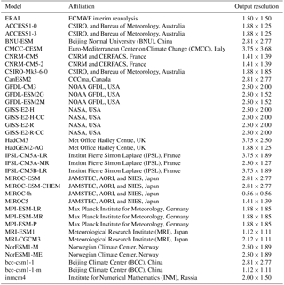
Table 1ERAI and CMIP5 models' affiliations and the horizontal resolution of the analyzed data (long lat∘). The first ensemble member (“r1i1p1”) is used from each CMIP5 model.
2.1 Data and code structure
The code documentation below applies to the MATLAB version of TropD. The syntax for the Python version (PyTropD) follows the MATLAB syntax and is documented in the Python code package. Although some of the metrics presented here may be used on zonally varying fields, we stress that the methodologies described here are designed for use on zonal-mean fields (the code has not been tested on zonally varying fields). Calculations in the TropD software assume pressure–latitude (hPa, latitude degrees) coordinates where the pressure level closest to the top of the atmosphere and the latitude grid point nearest to the southern pole are the first elements in the vertical and meridional ordinates, respectively. To reduce sensitivity to format variations across datasets, this ordering is automatically enforced in TropD.
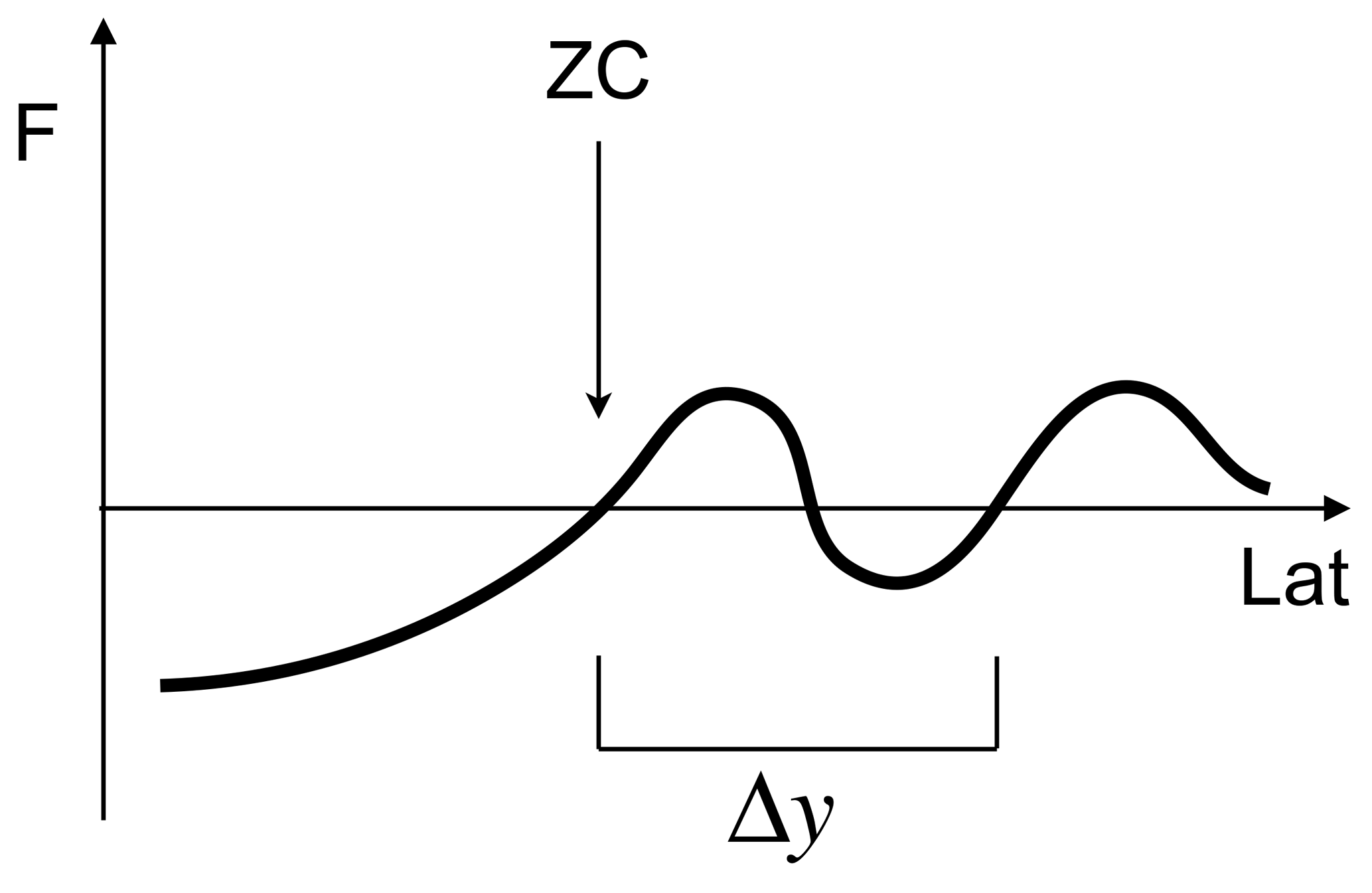
Figure 1A depiction of the latitude of the zero crossing ZC of some
field F along the interval lat. The distance to the nearest
zero crossing with the same sign change is denoted by Δy.
TropD is divided into auxiliary calculation functions, generically named
TropD_Calculate_[FunctionName], and metric functions, named
TropD_Metric_[MetricName]. Example code is provided in the file
TropD_Example_Calculations. TropD includes monthly zonal-mean data
and precalculated metrics derived from ERAI (for default values of the
metric functions) which can be used to run the example code and validate
calculations on different machines or versions of the programming language.
2.2 Calculating the latitude of zero crossing
The calculation of the zero-crossing latitude of some function can be generalized to the crossing of any cutoff value by raising or lowering the function by a constant. Therefore, all calculations involving cutoff criteria are translated in TropD to the basic operation of calculating the zero-crossing latitude of some field.
The following guidelines are implemented in calculations of the latitude of zero crossing:
- i.
Unless the zero crossing occurs at a grid point, the exact latitude of the zero crossing is calculated using linear interpolation between the two nearest data points on either side of the zero crossing.
- ii.
In cases where multiple zero-crossing latitudes exist, the first zero crossing along the input interval is chosen.
- iii.
In cases where multiple zero-crossing latitudes exist, the calculation can be defined as invalid if the latitudinal spacing between the first zero crossing along the input interval and the second zero crossing of the same sign change is smaller than some defined value.
Comments on the code
The zero-crossing latitude is calculated in TropD using the following
syntax:>> ZC = TropD_Calculate_ZeroCrossing (F,lat,Lat_Uncertainty)
where ZC denotes the first latitude of zero crossing (i.e., sign
change) of the field F along the interval lat as
illustrated in Fig. 1. (The metric functions described below
automatically order the input interval lat such that the first
latitude of zero crossing in each hemisphere corresponds to the most
equatorward zero crossing.) The input parameter Lat_Uncertainty is
intended for cases where multiple zero crossings exist (optional and equal to
zero by default). It specifies the minimal allowed distance between the first
and second zero-crossing latitudes of the same sign change (Δy in
Fig. 1) along the interval lat. In the example shown in
Fig. 1, for Lat_Uncertainty=10 (∘), ZC is output
as “not a number” (NaN) if Δy<10, and as the first zero crossing
along lat if Δy≥10. Likewise, ZC is output as
NaN when a zero crossing does not exist along the interval lat.

Figure 2Example of the latitude of the maximum (Ymax) of a field
F, calculated using TropD_Calculate_MaxLat(F,lat,n).
F is given as some skewed Gaussian function (black) with random
noise (blue) on a discretized grid with a random resolution. The results for
n=6 (red) and n=30 (green) are indicated by vertical lines.
The absolute maximum is indicated by a dot (magenta).
2.3 Calculating the latitude of the maximum
To account for potential noise in the data and to reduce grid dependence, the latitude of the maximum ϕmax of some field F is calculated using
where ϕ denotes latitude, ϕ1 and ϕ2 denote meridional boundaries, F is positive everywhere, and n≥1 (Adam et al., 2016). For n=1, Eq. (1) yields the centroid of F (e.g., as in the mass-weighted wind calculation of Archer and Caldeira, 2008), and for it yields the exact latitude of maximum of F. The exponent n therefore acts as a smoothing parameter with maximal smoothing for n=1 and no smoothing for . Based on Monte Carlo simulations of randomized skewed Gaussian functions on randomized grid spacing and with randomized noise (an example of such a random function is shown in Fig. 2), we find that the latitude of the maximum is identified most reliably for n≥6. The dependence of the error distribution on n is shown for a representative sample of 100 random functions in Fig. 3. The standard deviation of the error decreases with increasing n and remains minimal for n≥6. However, the probability of large error (i.e., the probability of outlier results) increases with n for n≥6.
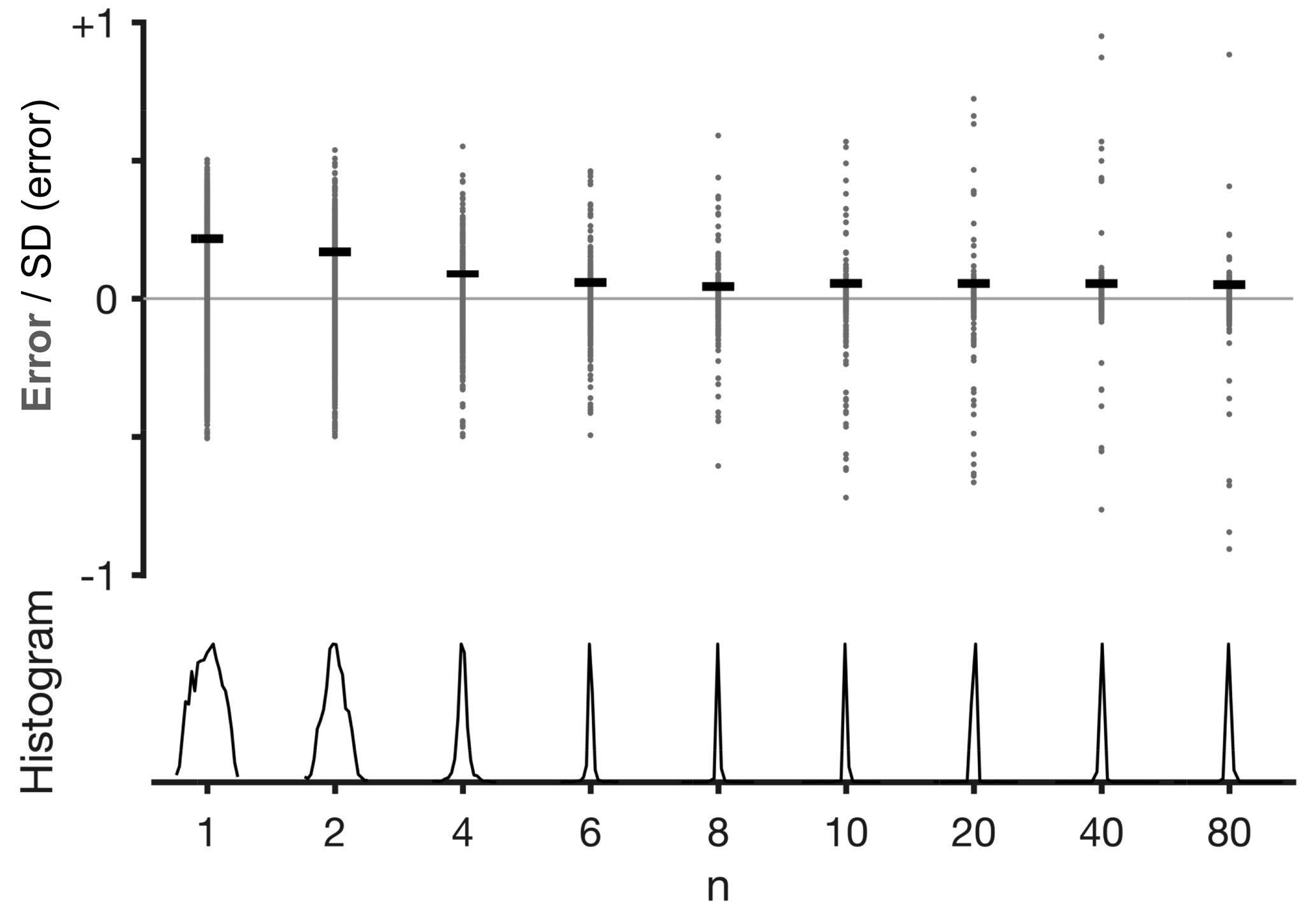
Figure 3The dependence on n of the error distribution of
ϕmax calculated using Eq. (1) in a representative sample of
100 randomized skewed Gaussian functions such as the one shown in
Fig. 2. The error (gray dots) is defined as the difference between
ϕmax and the latitude of the maximum of the smooth Gaussian function
(black line in Fig. 2). SD (error) (standard deviations of the error), horizontal lines, and histograms (normalized between 0 and 1) are shown for
the error distributions of the sample for each n.
Comments on the code
The latitude of the maximum is calculated in TropD using the following
syntax:>> Ymax = TropD_Calculate_MaxLat(F,lat,n)
where Ymax denotes the calculated latitude of the maximum, and
F is some field along the interval lat as illustrated in
Fig. 2. In order to avoid rounding errors and in order to make the
field F positive everywhere, F is normalized between zero
and one prior to applying Eq. (1), which is calculated using
trapezoidal integration along lat. The input field F is
therefore not required to be positive everywhere. In addition, F may
include NaN values; i.e., TropD ignores NaN values in the integral of
F in Eq. (1). The exponent n is an optional input
parameter (n ≥1), set to 6 by default. In the various
implementations of the metric methods described below, the function
TropD_Calculate_MaxLat is employed in two possible configurations:
- i.
max: corresponding ton=6(moderate smoothing) and - ii.
peak: corresponding ton=30(weak smoothing), which yields a latitude nearly equal to the latitude of absolute maximum ofF(Fig. 2).
The differences between these two configurations and the sensitivity of the
different metrics to the value of n are discussed further in
Sect. 4.
In this section, we provide technical guidelines for common methodologies in each of the eight metric categories. We briefly introduce each of the tropical-width metric categories below. For extended reviews of the physical rationale and interrelations of these metrics in various datasets, see Davis and Rosenlof (2012), Solomon et al. (2016), Davis and Birner (2017), and Waugh et al. (2018).
3.1 PSI – meridional mass stream function
The tropical mean meridional overturning circulation (i.e., the Hadley cells) can be defined as the tropical circulation enclosed within the zero streamlines of the zonal-mean meridional mass stream function ψ. A common tropical-width metric is therefore the subtropical latitude in each hemisphere where ψ changes sign poleward of the tropical stream function extrema.
The meridional mass stream function satisfies the continuity equation such that
Here, v and w denote the meridional and vertical (pressure velocity) components of the zonal-mean wind, g is the gravitational constant, a denotes Earth's radius, and p denotes pressure. Since the vertical velocity is not a well-observed quantity, ψ is commonly calculated as the vertical integral of the meridional component of the zonal-mean wind,
For most ψ-based metrics, spurious uncertainty related to the representation of subsurface data in the dataset (i.e., where p is larger than the surface pressure) can be avoided by ensuring Eq. (3) is numerically integrated from the top of the atmosphere. The units of ψ calculated using Eq. (3) are kg s−1 (the annual-mean intensity of the Hadley circulation is roughly 1011 kg s−1). Divided by the density of water (1000 kg m−3), ψ is often presented in Sverdrup units (1 Sv =106 m3 s−1), which are equivalent to 109 kg s−1.
3.1.1 Methods
The most widely used ψ-based metric of the tropical width is the zero-crossing latitude of the stream function at the 500 hPa level, poleward of the stream function extremum in each hemisphere. In order to reduce sensitivity to vertical variations in the stream function, some studies vertically average the stream function in the troposphere (e.g., between the 400 and 600 hPa levels; Hu and Fu, 2007) or, assuming stratospheric contributions can be neglected, vertically average across the entire atmospheric column (e.g., Davis and Birner, 2017). Similarly, in order to avoid ambiguity due to multiple subtropical zero-crossing latitudes, the edge of the Hadley cell is defined in some studies as the first latitude at which the stream function decreases to some fraction (e.g., 10 %) of its extremal value in each hemisphere or to some minimal threshold value (e.g., 25 Sv; Levine and Schneider, 2011).
3.1.2 Comments on the code
The stream function is calculated in TropD using the following syntax:>> Psi = TropD_Calculate_StreamFunction (V,lat,lev) where
Psi is the zonal-mean stream function, V is the zonal-mean
meridional wind, and lat and lev are the latitude and
pressure-level vectors. The stream function is calculated using
Eq. (3) by trapezoidal integration from the smallest to highest
pressure levels.
The PSI metric is calculated in TropD using the following syntax:>> [Ys Yn] = TropD_Metric_PSI(V,lat,lev, method,Lat_Uncertainty,Levels) where
V(lat,lev) is the zonal-mean meridional wind. As in all of the
metrics described below, Ys and Yn are the tropical edge
latitudes in the Southern Hemisphere and Northern Hemisphere (SH and NH), respectively,
and lat and lev are the meridional and vertical ordinates,
respectively. The input variable Levels (optional) is a scalar or
two-element vector which specifies upper and lower pressure-level boundaries
(in hPa). The default value of the input parameter Lat_Uncertainty
(optional), used by the function TropD_Calculate_ZeroCrossing as
described above, is zero. The PSI metric can be calculated using several
implemented methods, specified by the method string (optional, not
required for default methods), which are the following:
- i.
Psi_500(default) is the zero crossing of ψ at the 500 hPa pressure level. - ii.
Psi_500_10Percis the first latitude at which ψ at the 500 hPa pressure level decreases to 10 % of its extremal tropical value in each hemisphere. - iii.
Psi_Levelsis the zero crossing of ψ integrated between two pressure levels, specified byLevels. The default values of the lower and upper pressure levels are 700 and 300 hPa. If a single pressure level is specified byLevels, the metric function will output the zero crossing of ψ at the specified pressure level. For example,>> [Ys Yn] = TropD_Metric_PSI(V,lat, lev,`Psi_Levels',0,[400 600])will output the zero crossing of ψ integrated between the 400 and 600 hPa levels. The calculation is not sensitive to the ordering of the pressure levels inLevels(i.e., settingLevels = [400 600]orLevels = [600 400]produces the same result). Similarly, settingLevels = [500 500]orLevels=500will produce a result identical to selecting the methodPsi_500. If the pressure levels specified byLevelsare not a subset oflev, the pressure levels closest to the ones specified inLevelsare used in the calculation. - iv.
Psi_500_Intis the zero crossing of ψ integrated between the top of the atmosphere and the 500 hPa pressure level. - v.
Psi_Intis the zero crossing of ψ integrated between the top and surface.
For all of the above methods, the edge latitude is calculated as the most equatorward latitude where the method criteria are met, poleward of the stream function extremum in each hemisphere.
3.2 TPB – tropopause break
The tendency of the tropopause height to abruptly drop near the subtropical jet (e.g., Fig. 4a) is often used to diagnose the tropical width. The commonly accepted definition of the tropopause follows the World Meteorological Organization (WMO, 1957): the lowest point at which the lapse rate decreases to 2 K km−1 and remains lower than 2 K km−1 between this level and all higher levels within 2 km. The manner in which the latter part of the WMO definition is implemented has been shown to potentially influence the evaluation of observed trends (Birner, 2010). In addition, indirect measurements of the tropopause break derived from changes in column ozone concentrations have been shown to detect secular trends consistent with thermodynamic TPB metrics (Hudson et al., 2006). However, metrics based on ozone concentrations exhibit strong sensitivity to the methodology applied (Davis et al., 2018) and are therefore not considered here.
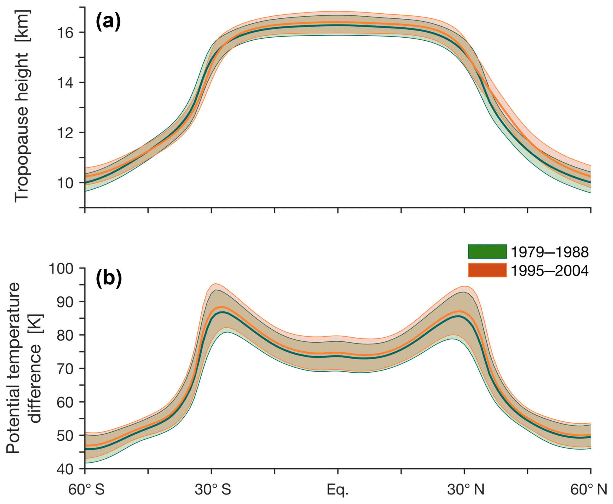
Figure 4The mean tropopause height (a) and the difference in the potential temperature between the tropopause level and the surface (b) during the decades beginning in 1979 (green) and 1995 (orange) in CMIP5 models. The shading indicates ±1 standard deviation of inter-model spread. The calculations are derived from monthly means of the temperature field.
3.2.1 Methods
Various tropopause-based methods for calculating the zonal-mean width of the tropics are found in the literature. These generally include
- i.
the latitude of the largest negative poleward gradient in the tropopause height (e.g., Davis and Rosenlof, 2012; Davis and Birner, 2017);
- ii.
the most poleward latitude where the number of days per year with tropopause heights above a certain altitude exceeds some threshold (e.g., Seidel and Randel, 2007);
- iii.
the latitude at which the tropopause height drops below a certain fixed threshold, or a threshold that depends on the mean properties of the tropical tropopause (Birner, 2010; Davis and Rosenlof, 2012); and
- iv.
the latitude of maximal difference between the potential temperature at the tropopause and at the surface (Fig. 4b; Davis and Birner, 2013, 2017)
Each of these methodologies present potential weaknesses. For example, threshold-based metrics are sensitive to the choice of threshold values (e.g., Birner, 2010), and the latitude of maximal gradient is sensitive to noise and grid spacing (e.g., Davis and Rosenlof, 2012). It is therefore particularly important to consider the TPB metric method most suited to the data being analyzed and the physical question being addressed.
3.2.2 Comments on the code
The tropopause height is calculated in TropD using the following syntax:>> Pt = TropD_Calculate_TropopauseHeight (T,p)
where Pt is the zonal-mean tropopause pressure (hPa) derived from
the zonal-mean temperature T(lat,lev) and the vertical pressure
levels p(lev) using the method described in Reichler et al. (2003). The
implementation of the 2 km condition in accordance with the WMO definition
is as described in Birner (2010). It is possible to output the value of
some field at the tropopause level, using the following syntax:>> [Pt Ht] = TropD_Calculate_ TropopauseHeight(T,p,Z)
where Ht is the value of the field Z(lat,lev), with
identical dimensions to T(lat,lev), evaluated at the tropopause
pressure level (by linear interpolation).
The TPB metric is calculated in TropD using the following syntax:>> [Ys Yn] = TropD_Metric_TPB(T,lat,lev, method,Z,Cutoff) The above-mentioned methodologies for calculating the TPB metric can be
realized in TropD by specifying the method string:
- i.
max_gradient(default) is the latitude of maximal poleward gradient of the tropopause pressure, using the syntax>> [Ys Yn] = TropD_Metric_TPB(T,lat, lev,`max_gradient')
with the smoothing parametern=6. - ii.
max_potempis the latitude of maximal difference between the potential temperature at the tropopause and the minimal value of the potential temperature in each latitude column (assumed to be located at the surface), using the syntax>> [Ys Yn] = TropD_Metric_TPB(T, lat,lev,`max_potemp')
with the smoothing parametern=30. - iii.
cutoffis the most equatorward latitude where some fieldZ, evaluated at the tropopause level, crosses some cutoff valueCutoff, using the syntax>> [Ys Yn] = TropD_Metric_TPB(T,lat,lev, `cutoff',Z,Cutoff)
The default value of the cutoff parameterCutoffis 15 000, assuming the input fieldZis geopotential height in units of meters.
The default smoothing parameter values in the max_gradient and
max_potemp methods are based on the analysis described in
Sect. 4.3. For these methods, the value of n can be set as an input
scalar
(n ≥1) after the method string; i.e.,>> [Ys Yn] = TropD_Metric_TPB(T,lat,lev, `max_gradient',n)
or >> [Ys Yn] = TropD_Metric_TPB(T,lat,lev, `max_potemp',n).
The tropopause break latitude is calculated equatorward of 60∘ for
all of the methods. The method described in Seidel and Randel (2007) and similar
methods which require some statistical analysis of the tropopause time series
are not explicitly implemented in TropD. Instead, the various methods
implemented in TropD (e.g., the cutoff method) are designed to
facilitate such calculations in a manner that is consistent across analyses.
3.3 OLR – outgoing longwave radiation
Due to variations in atmospheric absorption and surface temperature, the longwave radiation emitted to space maximizes in the subtropics (∼270 W m−2 in the zonal mean; Fig. 5a), coinciding with the dry subsiding branches of the Hadley circulation. This, together with the existence of direct satellite observations of OLR, has motivated the use of OLR-based metrics for evaluating tropical-width variations (e.g., Hu and Fu, 2007).
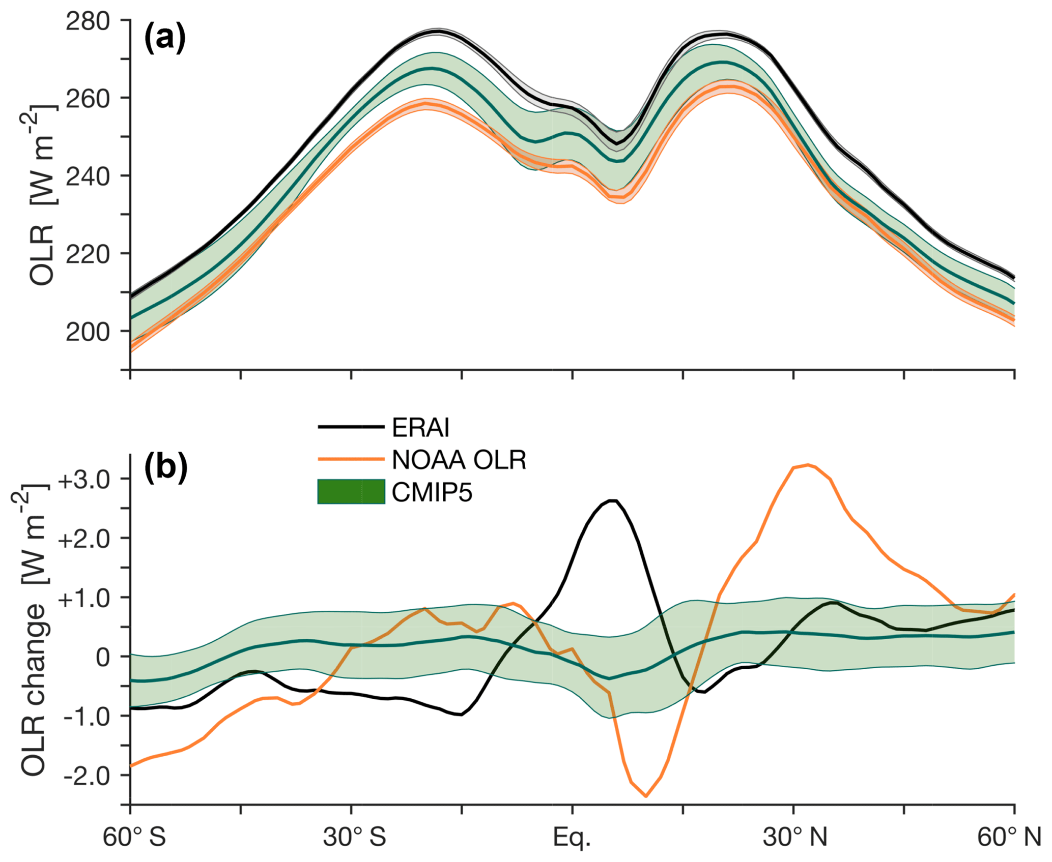
Figure 5Outgoing longwave radiation (OLR) at the top of the atmosphere in CMIP5 models (green), ERAI (black), and the National Oceanic and Atmospheric Administration (NOAA) interpolated OLR dataset (orange; Liebmann and Smith, 1996). (a) The mean OLR during 1979–2004. (b) The difference in OLR between the decades beginning in 1995 and 1979. The shading indicates ±1 standard deviation of inter-model spread for CMIP5 models and of interannual variations for ERAI and the NOAA interpolated OLR.
3.3.1 Methods
Common OLR-based methods for calculating the tropical width are
- i.
the most poleward latitude at which the zonal-mean OLR is equal to 250 W m−2 (e.g., Hu and Fu, 2007; Johanson and Fu, 2009), and
- ii.
the first latitude poleward of the subtropical OLR maximum at which the zonal-mean OLR drops to 20 W m−2 below its peak value in each hemisphere (Davis and Rosenlof, 2012).
3.3.2 Comments on the code
For generality, several OLR metric methods are implemented in TropD, using
the following syntax:>> [Ys Yn] = TropD_Metric_OLR(OLR,lat, method,options)
where OLR(lat) is the zonal-mean OLR. The methods are as follows:
- i.
250W(default) is the most equatorward latitude at which OLR drops below 250 W m−2, poleward of the subtropical OLR maximum in each hemisphere. - ii.
cutoffis the most equatorward latitude, poleward of the subtropical OLR maximum in each hemisphere, at which OLR drops below a certain cutoff value specified by the parameterCutoff:>> [Ys Yn] = TropD_Metric_OLR(OLR,lat, `cutoff',Cutoff)
The default value of the parameterCutoffis 250 (W m−2; i.e., thecutoffand250Wmethods are identical ifCutoffis not specified). - iii.
20Wis the most equatorward latitude, poleward of the subtropical OLR maximum in each hemisphere, at which OLR drops to 20 W m−2 below the OLR maximum. - iv.
10Percis the most equatorward latitude, poleward of the subtropical OLR maximum in each hemisphere, at which OLR drops to 90 % of the OLR maximum. - v.
maxis the latitude of maximal OLR in each hemisphere, calculated usingTropD_Calculate_MaxLatwith the smoothing parametern=6. The value ofncan be set as an input scalar (n≥1) after the method string; i.e.,>> [Ys Yn] = TropD_Metric_OLR(OLR,lat, `max',n) - vi.
peakis the latitude of maximal OLR in each hemisphere, calculated usingTropD_Calculate_MaxLatwith the smoothing parametern=30.
The flexibility in the input parameters n and Cutoff in the
OLR metric function is designed to enable sensitivity testing of this metric,
as well as other metrics based on one-dimensional zonal-mean fields.
3.4 STJ – subtropical jet
In idealized theory, the subtropical jets form at the edges of the poleward-moving upper tropospheric branches of the Hadley circulation in each hemisphere (e.g., Schneider, 2006). This motivates the use of the latitude of the subtropical jet as an indicator of the tropical width. However, upper-level winds are also strongly affected by midlatitude macroturbulence and stratospheric processes, obliging caution in associating the latitude of maximal zonal wind with the above conceptual picture of the latitude of the subtropical jet. Indeed, recent studies find that STJ-based metrics of the tropical width are weakly correlated with lower-troposphere metrics (Solomon et al., 2016; Davis and Birner, 2017). Common STJ-based metrics take into consideration the characteristics of the upper-level zonal winds in various ways, as described below.
3.4.1 Methods
Accounting for the fact that the STJs exhibit significant variations in longitude and altitude, the latitude of the STJ as an indicator of the tropical width has been generally calculated in the literature as
- i.
the centroid of the upper-level zonal wind within a specified meridional band (e.g., the vertical average of the zonal wind between the 100 and 400 hPa levels in the 15–70∘ latitude band; Archer and Caldeira, 2008);
- ii.
the latitude of the maximum of the upper-level zonal wind (e.g., averaged between the 100 and 400 hPa levels; Davis and Rosenlof, 2012; Solomon et al., 2016); and
- iii.
the latitude of the maximum of the upper-level minus lower-level zonal wind. As shown in Fig. 6, the subtraction of the lower-level wind differentiates the signal of the STJ from that of the midlatitude eddy-driven jet, which is characterized by stronger vertical homogeneity (Davis and Birner, 2016, 2017).
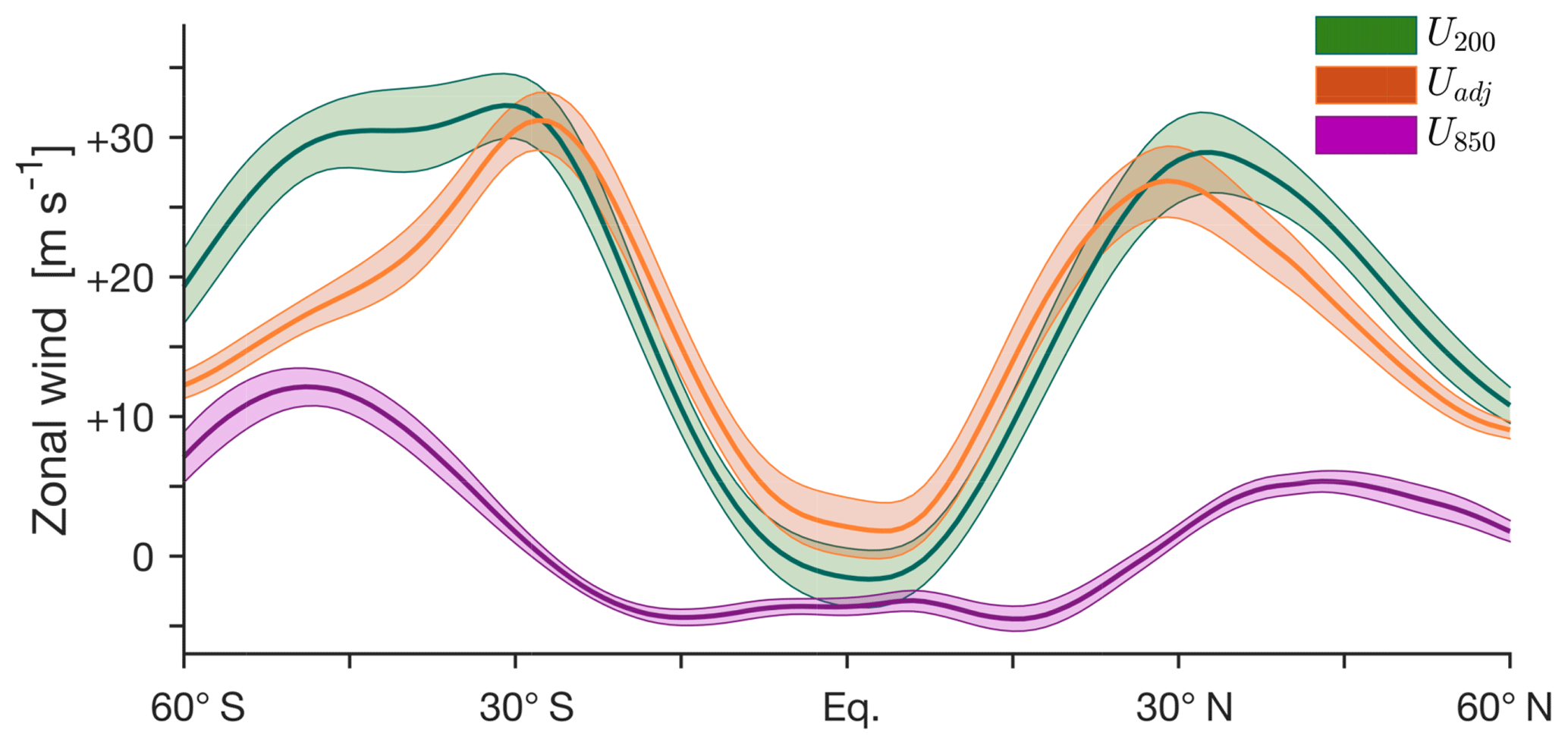
Figure 6The zonally averaged annual-mean zonal wind at the 200 and 850 hPa levels (U200, green, and U850, purple) and the difference between U200 and U850 (Uadj, orange). Data are taken from CMIP5 models for 1979–2004. The shading indicates ±1 standard deviation of inter-model spread.
3.4.2 Comments on the code
The STJ metric is calculated in TropD using the following syntax:>> [Ys Yn] = TropD_Metric_STJ(U,lat,lev, method,n)
where U(lat,lev) denotes the zonal-mean zonal wind. The available methods are
- i.
adjusted_peak(default): the latitude of the maximum of the zonal wind averaged between the 100 and 400 hPa levels minus the zonal wind at the 850 hPa level (smoothing parametern=30); - ii.
adjusted_max: the latitude of the maximum of the zonal wind averaged between the 100 and 400 hPa levels minus the zonal wind at the 850 hPa level (smoothing parametern=6); - iii.
core_peak: the latitude of the maximum of the zonal wind averaged between the 100 and 400 hPa levels (smoothing parametern=30); and - iv.
core_max: the latitude of the maximum of the zonal wind averaged between the 100 and 400 hPa levels (smoothing parametern=6).
In all of the above methods, the latitude of the maximum is calculated
poleward of 10∘ and equatorward of 60∘ for the core
methods and equatorward of the latitude of the maximum of the zonal wind at
the 850 hPa level in each hemisphere (i.e., equatorward of the eddy-driven
jet; see below) for the adjusted methods. To reduce sensitivity to
pressure-level spacing, vertical averages are pressure weighted
(cf. Archer and Caldeira, 2008; Davis and Rosenlof, 2012). For all of the above
methods, inputting the value of n is optional and overrides the
default values (i.e., 6 for max and 30 for peak).
3.5 EDJ – eddy-driven jet
The macroturbulent eddy momentum fluxes in midlatitudes, which drive the midlatitude jets, affect the zonal-mean overturning circulation and therefore the tropical width (Kim and Lee, 2001; Schneider, 2006). Indeed, under some conditions, strong correlations are found between the positions of the EDJs and the width of the Hadley circulation, in particular in the SH during the summer months (Kang and Polvani, 2011). Since, in contrast to the STJs, the midlatitude EDJs are characterized by relatively strong near-surface westerlies, EDJ-based metrics are generally calculated as the latitude of the maximum of near-surface westerlies (e.g., Woollings et al., 2010; Kang and Polvani, 2011; Davis and Birner, 2017).
3.5.1 Methods
To reduce grid dependence, it is common practice to fit a quadratic polynomial onto data from grid points surrounding the grid point of the maximum, and define the position of the EDJ as the latitude of the maximum of that polynomial (e.g., Kidston and Gerber, 2010; Solomon et al., 2016). Davis and Birner (2017) use a linear interpolation of the gradient of the zonal-mean zonal wind at 850 hPa to estimate the position of the EDJ. For consistency, the preferred methodology of the EDJ metric in TropD uses Eq. (1). For reference with previous studies, a generalized method based on a quadratic polynomial fit is also included.
3.5.2 Comments on the code
The EDJ metric is calculated in TropD using the following syntax:>> [Ys Yn] = TropD_Metric_EDJ(U,lat,lev, method)
where U(lat,lev) denotes the zonal-mean wind. The methods are
- i.
peak(default): the latitude of the maximum of the zonal wind at the level closest to 850 hPa (smoothing parametern=30); - ii.
max: the latitude of the maximum of the zonal wind at the level closest to 850 hPa (smoothing parametern=6); and - iii.
fit: the latitude of the maximum of a quadratic polynomial fit usingmgrid points on either side of the grid point of maximal zonal wind at the level closest to 850 hPa. The default value ofmis 1.
The values of the smoothing parameter n in the max and
peak methods (n ≥1) and of the number of grid points
on either side of the polynomial fit in the fit method (m =
) can be set as an input scalar after the method string;
e.g.,>> [Ys Yn] = TropD_Metric_EDJ(U,lat,lev, `max',n)
or>> [Ys Yn] = TropD_Metric_EDJ(U,lat,lev, `fit',m)
In all of
the above EDJ methods, the latitude of the maximum is calculated poleward of
15∘ and equatorward of 70∘ (i.e., slightly poleward of
60∘, which is the poleward boundary in all of the other metrics).
3.6 PE – precipitation minus evaporation
The subtropical dry zones lie at the latitude bands of the descending
branches of the tropical meridional overturning circulation. The poleward
edges of the subtropical dry zones can therefore be used as indices of the
tropical width (e.g., Lu et al., 2007). The PE metric is calculated in TropD
using the following syntax:>> [Ys Yn] = TropD_Metric_PE(PE,lat, method,Lat_Uncertainty)
where PE(lat) denotes the zonal-mean precipitation minus evaporation
field (Fig. 7a). The default and only available method is
zero_crossing, which calculates the zero-crossing latitude poleward
of the subtropical minimum in PE and equatorward of 60∘. The
default value of the input parameter Lat_Uncertainty (optional),
used by the function TropD_Calculate_ZeroCrossing as described
above, is zero.
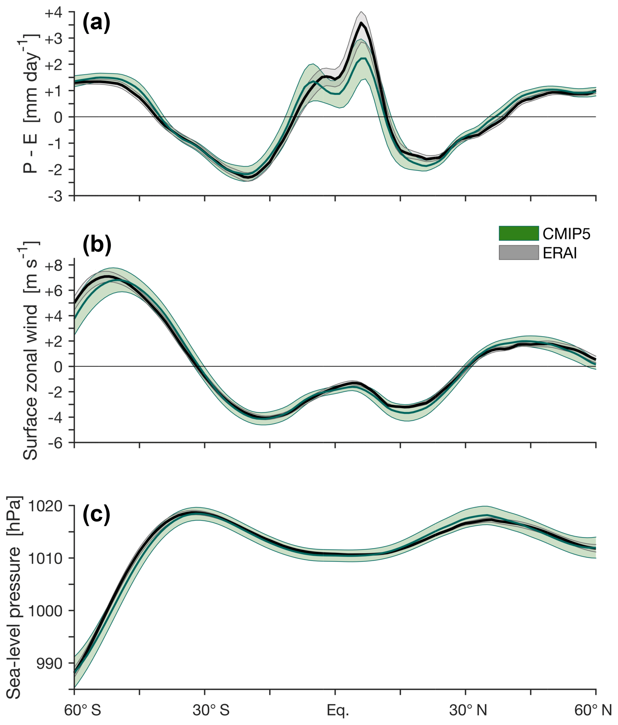
Figure 7Zonally averaged annual-mean values of (a) precipitation minus evaporation (P−E), (b) surface zonal wind, and (c) sea-level pressure in CMIP5 models (green) and ERAI (black) for 1979–2004. The shading indicates ±1 standard deviation of inter-model spread for CMIP5 models and of interannual variations for ERAI.
3.7 UAS – near-surface zonal wind
The edge of the tropics is characterized by a transition from surface
easterlies in the equatorward-flowing lower tropospheric branch of the Hadley
circulation to surface westerlies in midlatitudes (Fig. 7b). In
steady state, the zonal-mean column-averaged zonal momentum flux divergence
is balanced by surface drag. Therefore, the subtropical latitude where the
zonal surface wind changes sign (i.e., where surface drag vanishes) also
indicates the latitude where eddy and mean momentum flux divergences balance
at higher levels (Held, 2000; Korty and Schneider, 2008). Analyses of the zero-crossing
latitude of surface zonal wind are generally insensitive to the exact
definition of the surface wind (e.g., the average wind 2 or 10 m above
surface, or the interpolated wind at the 1000 hPa level; Davis and Birner, 2017).
Therefore, the UAS metric is calculated in TropD as the zero-crossing
latitude of the zonal-mean near-surface zonal wind. The default and only
available UAS metric method is zero_crossing, which calculates the
zero-crossing latitude poleward of the subtropical minimum in each hemisphere
and equatorward of 60∘. The default value of the input parameter
Lat_Uncertainty (optional), used by the function
TropD_Calculate_ZeroCrossing as described above, is zero. The
syntax for the UAS metric is>> [Ys Yn] = TropD_Metric_UAS(U,lat, method,Lat_Uncertainty)
where U(lat) denotes the zonal-mean near-surface zonal wind (e.g.,
the wind 2 or 10 m above the surface, or the wind at some level below
850 hPa).
3.8 PSL – maximum sea-level pressure
The subtropical high-pressure belts form along the descending branches of the tropical meridional overturning circulation. The latitude of maximum sea-level pressure may therefore serve as a tropical width indicator (Hu et al., 2011; Choi et al., 2014). (The use of sea-level pressure as opposed to surface pressure limits the influence of elevation over continents.) In addition, sufficiently far from the Equator, the geostrophically balanced zonal wind changes sign where the meridional pressure gradient changes sign. Therefore, the latitude of maximum sea-level pressure lies near the latitude where the zonal-mean zonal surface wind changes sign (i.e., it is closely related to the UAS metric; Choi et al., 2014), particularly in the SH (Fig. 7; Waugh et al., 2018). To reduce grid dependence, several studies have used procedures which rely on nonlinear interpolation to identify the position of the sea-level pressure maximum (e.g., Hu et al., 2011; Choi et al., 2014). For consistency, the methods for calculating the PSL metric in TropD are the same as for the EDJ metric:
- i.
max: the latitude of the maximum of sea-level pressure (smoothing parametern=6) and - ii.
peak(default): the latitude of the maximum of sea-level pressure (smoothing parametern=30).
The syntax for the PSL metric is>> [Ys Yn] = TropD_Metric_PSL(PSL,lat, method)
where PSL(lat) denotes zonal-mean sea-level pressure.
In both the max and peak methods, the latitude of the
maximum is calculated poleward of 15∘ and equatorward of 60∘.
As in the EDJ, STJ, and OLR metrics, the value of n can be set as an
input scalar (n ≥1) after the method string; e.g.,>> [Ys Yn] = TropD_Metric_PSL(PSL,lat, `max',n).
We proceed with a method sensitivity analysis for the eight metrics
implemented in TropD. For clarity, we use [metric]:[method] to
denote metric and method.
4.1 Temporal averaging
It is important to note that, since the basic operators (max finding and zero
crossing) applied in the metric calculations are not linear, the metric
calculations do not commute in space and in time. This is illustrated in
Fig. 8, where the PSI metric is calculated from monthly and annual
means. The annual means are calculated using the TropD function
TropD_Calculate_Mon2Season, which calculates seasonal means from
a monthly time series (see the example code and the documentation in the code
for syntax).
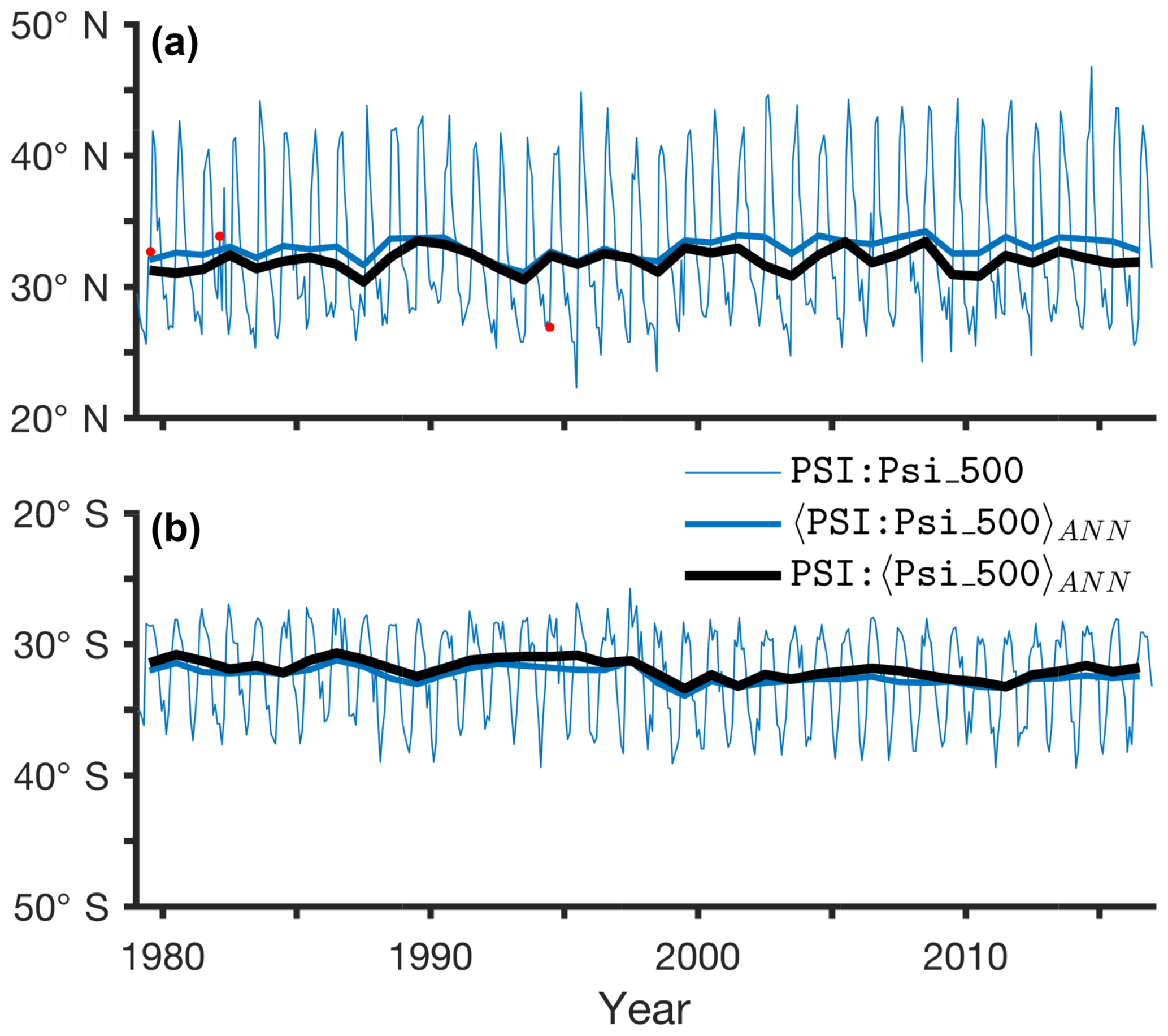
Figure 8Time series of the PSI metric for the Psi_500 method
(default) in the NH (a) and SH (b). Shown are monthly
values (thin blue), annual means of the monthly metric values (〈𝙿𝚂𝙸:𝙿𝚜𝚒_500〉ANN, thick blue), and metric values
derived from the annual-mean meridional wind (𝙿𝚂𝙸:〈𝙿𝚜𝚒_500〉ANN, black). Data are taken from ERAI for
1979–2016. The default value of the input parameter
Lat_Uncertainty is zero. Monthly values with invalid results for
Lat_Uncertainty=10 are marked by red dots (three in the NH and none in
the SH).
The annual means of PSI:Psi_500 derived from monthly means of v
(〈𝙿𝚂𝙸:𝙿𝚜𝚒_500〉ANN, blue line) clearly
differ from PSI:Psi_500 derived from annual means of v
(𝙿𝚂𝙸:〈𝙿𝚜𝚒_500〉ANN, black line).
The different seasonal averaging also yields slightly different decadal
trends in the NH and SH (0.27±0.21∘ decade−1 for the annual
mean of the metric derived from monthly means vs.
decade−1 for the metric derived from annual
means of v in the NH; and similarly, decade−1
vs. decade−1 in the SH; confidence bounds
indicate 5 % significance level using an F test).
The agreement between dynamically consistent metrics is found to improve when
these are derived from seasonal means as opposed to monthly means
(Waugh et al., 2018). Similarly, the application of the zero-crossing uniqueness
condition with Lat_Uncertainty=10 yields three invalid results for
monthly metric values in the NH but none for the metric values derived from
annual means (Fig. 8a) or seasonal means (not shown). Therefore, for
consistency in the analysis, we advocate that metrics should be calculated
from the seasonal means of the input field, as opposed to calculating the
seasonal means of the metric.
4.2 Grid dependence
To study the grid dependence of the various metric methods, we examine the relation of the interannual variability (the standard deviation of annual-mean values during 1979–2004) and the latitudinal grid spacing of the CMIP5 model output. Table 2 shows the inter-model correlation between the interannual variability and the latitudinal spacing for each of the metric methods. The grid dependence of the metric methods is generally higher in the SH, in particular for the near-surface metrics. This difference between the SH and NH may reflect smaller signal-to-noise ratio in the NH due to larger surface variability (i.e., it implies that grid dependence is more apparent in the SH, but not necessarily larger than in the NH). In addition, Davis and Birner (2016) find that (native) model resolution can affect eddy momentum and heat fluxes and therefore indirectly affect the large-scale circulation.
Table 2The Pearson coefficient of inter-model correlation between the interannual variability (defined as the standard deviation of annual-mean values for 1979–2004) of the metric and the latitudinal spacing of the model output in the 34 CMIP5 models. Default methods and statistically significant correlations (p<0.05) are bolded.
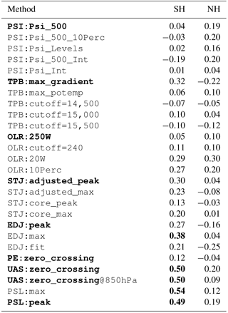
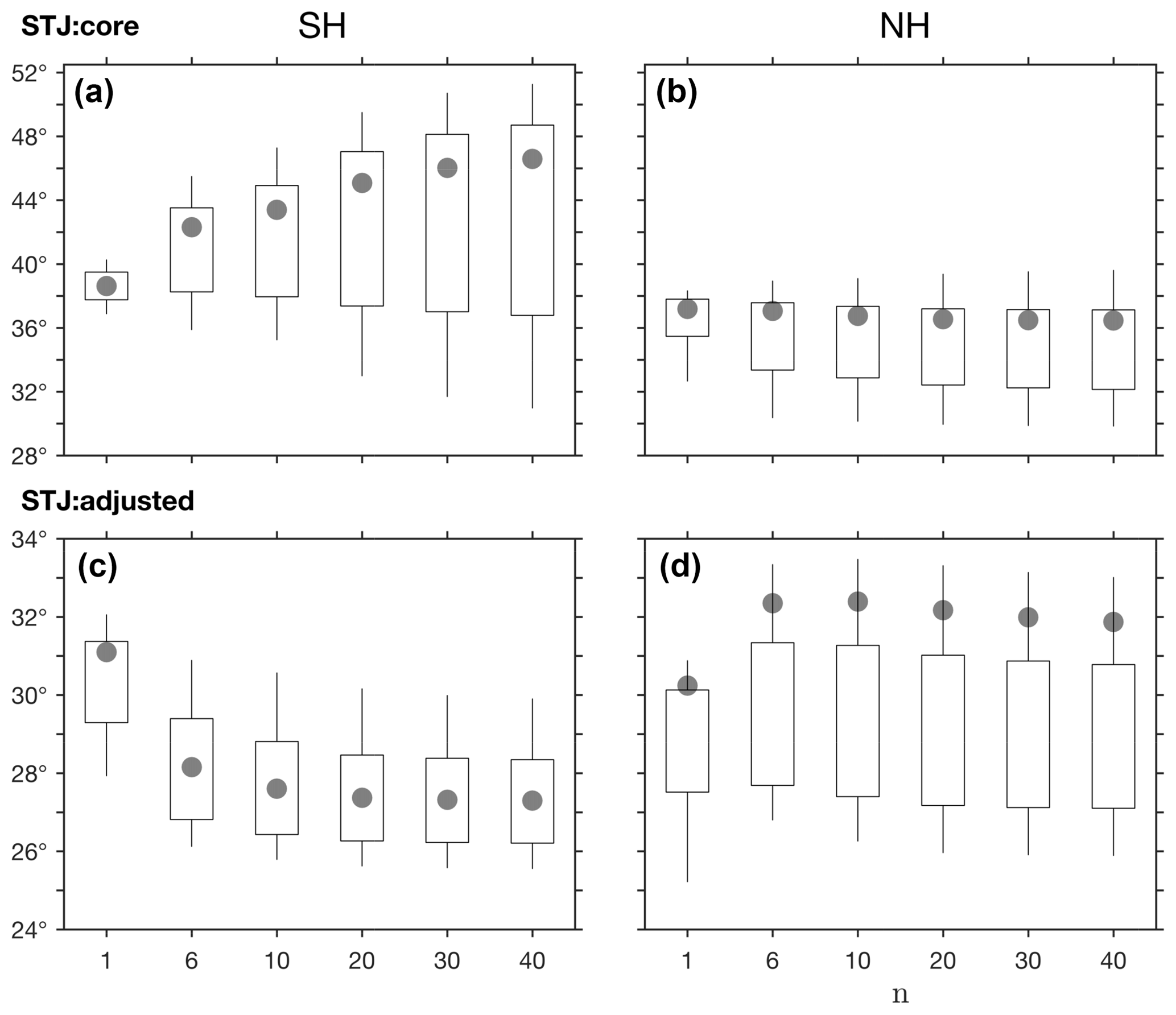
Figure 9The dependence of the mean metric latitude on the smoothing
parameter n for the STJ:core and STJ:adjusted
methods, derived from annual means of the zonal-mean zonal wind in the SH
(a, c) and NH (b, d), for the period 1979–2004. For
simplicity, positive values are used for both the NH and SH. Candle boxes
show mean ±1 standard deviation of CMIP5 inter-model spread (note,
however, that different vertical scales are used for STJ:core and
STJ:adjusted). Candle wicks show maximal and minimal CMIP5 model
values. ERAI values are shown in gray dots.
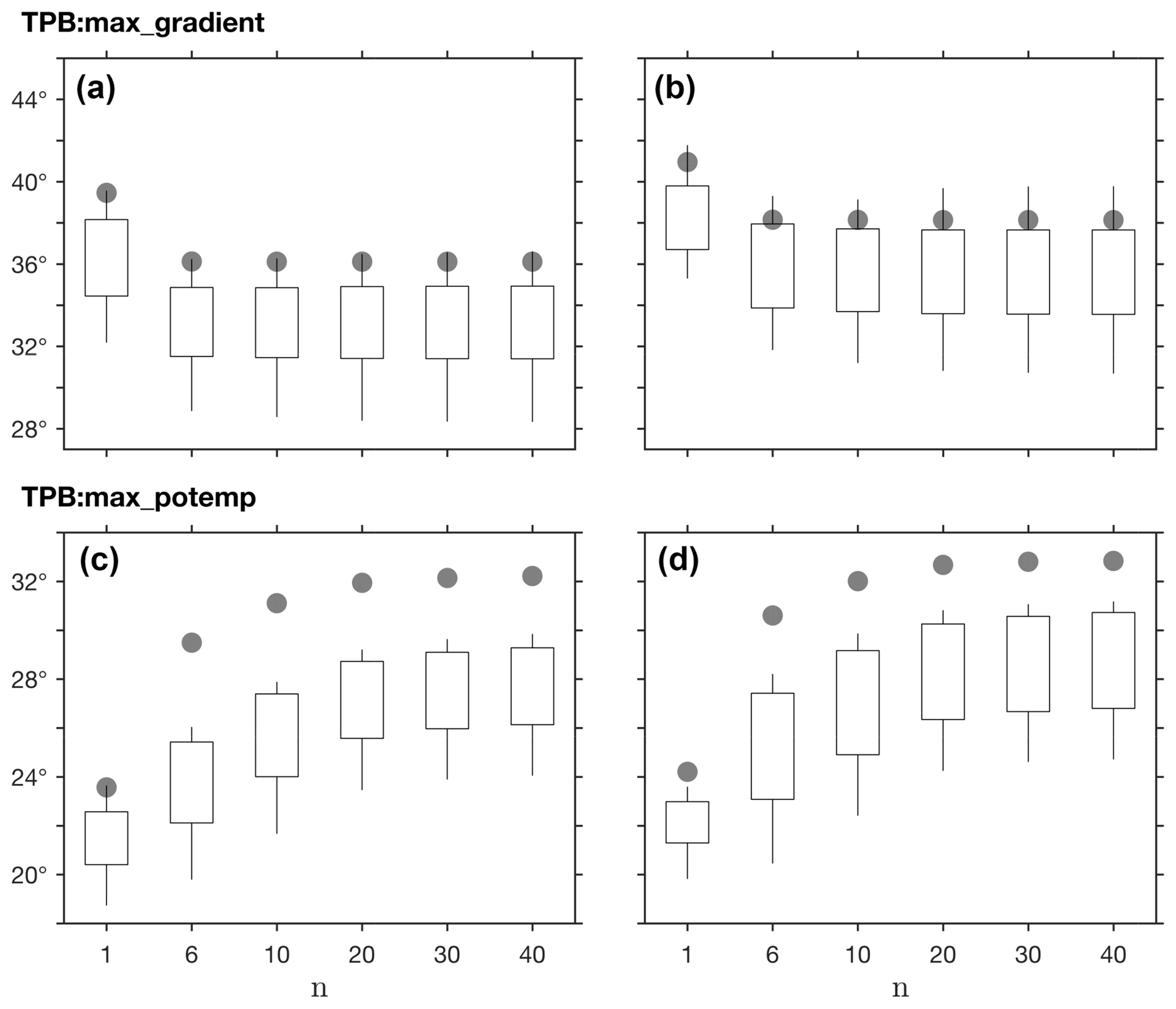
Figure 10As in Fig. 9 for the dependence of
TPB:max_gradient and TPB:max_potemp on the smoothing
parameter n.
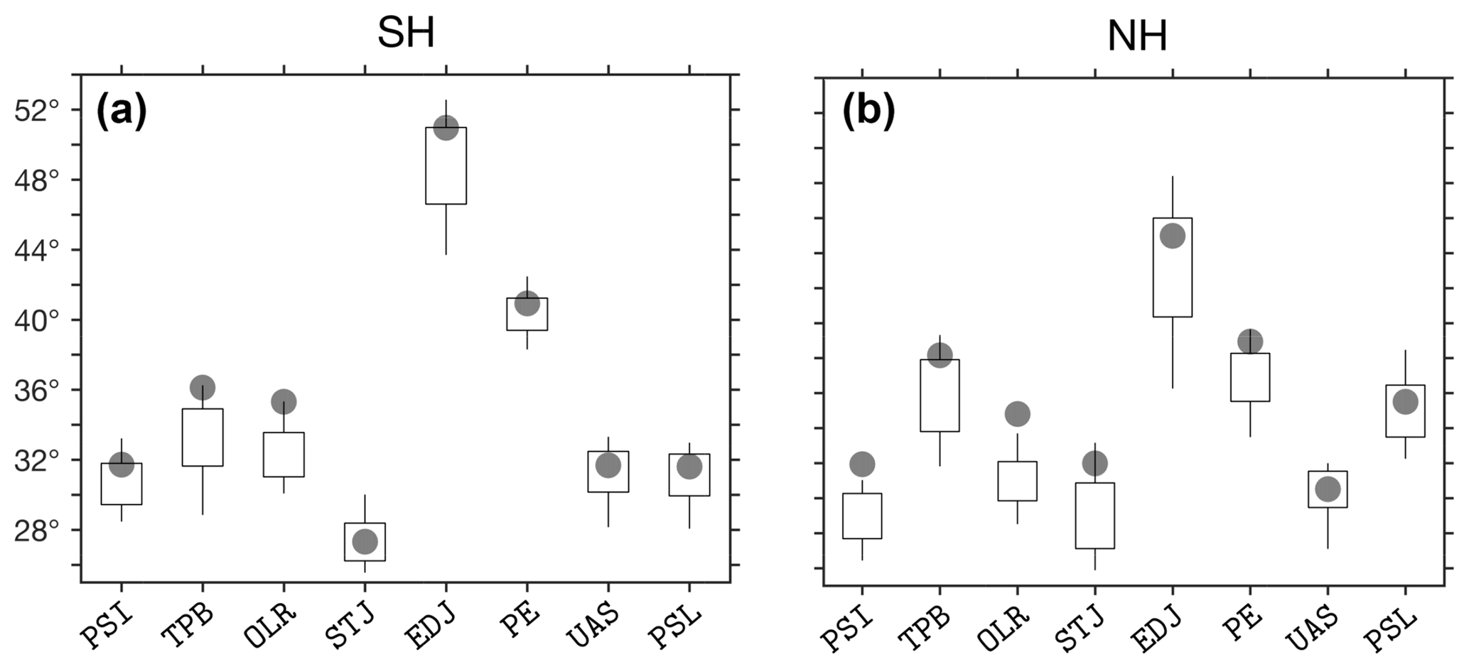
Figure 11The mean SH (a) and NH (b) latitudes of the
default methods in each of the eight metrics, derived from annual means, for
the period 1979–2004. Positive values are used for both the NH and SH.
Candle boxes show mean ±1 standard deviation of CMIP5 inter-model
spread. Candle wicks show maximal and minimal CMIP5 model values. ERAI values
are shown in gray dots. The input parameter Lat_Uncertainty is set
to zero (default) in all of the relevant methods.
Given this sensitivity to grid spacing, method and model selection can play a critical role in reducing the uncertainty in analyses of the tropical width. For example, the interannual variability of the CMCC-CESM model, which has the lowest latitudinal resolution of the CMIP5 models considered here (3.68∘, Table 1), is maximal or among the highest for most metrics, reflecting uncertainty in diagnosing the edge of the tropics rather than physical variability; excluding low-resolution models from analyses of the tropical width is therefore one way of reducing uncertainty. Likewise, in analyses of the tropical width that use data ensembles with large grid variance, uncertainty can be reduced by using metrics which are not sensitive to grid spacing (e.g., the PSI metric).
4.3 Sensitivity to the smoothing parameter n
In the presence of random noise, the max method which uses moderate
smoothing (n=6), and the peak method which uses weak
smoothing (n=30) and is therefore more sensitive to noise, can
produce significantly different estimates of the latitude of the maximum
(Fig. 3). However, in both observations and simulations, it is not
clear whether differences between the max and peak methods
reflect grid dependence, sensitivity to noise, or a realistic quantification
of physical variability. In other words, the optimal smoothing level, which
minimizes grid dependence and noise while retaining the relevant physical
properties of the analyzed variable, is not known.
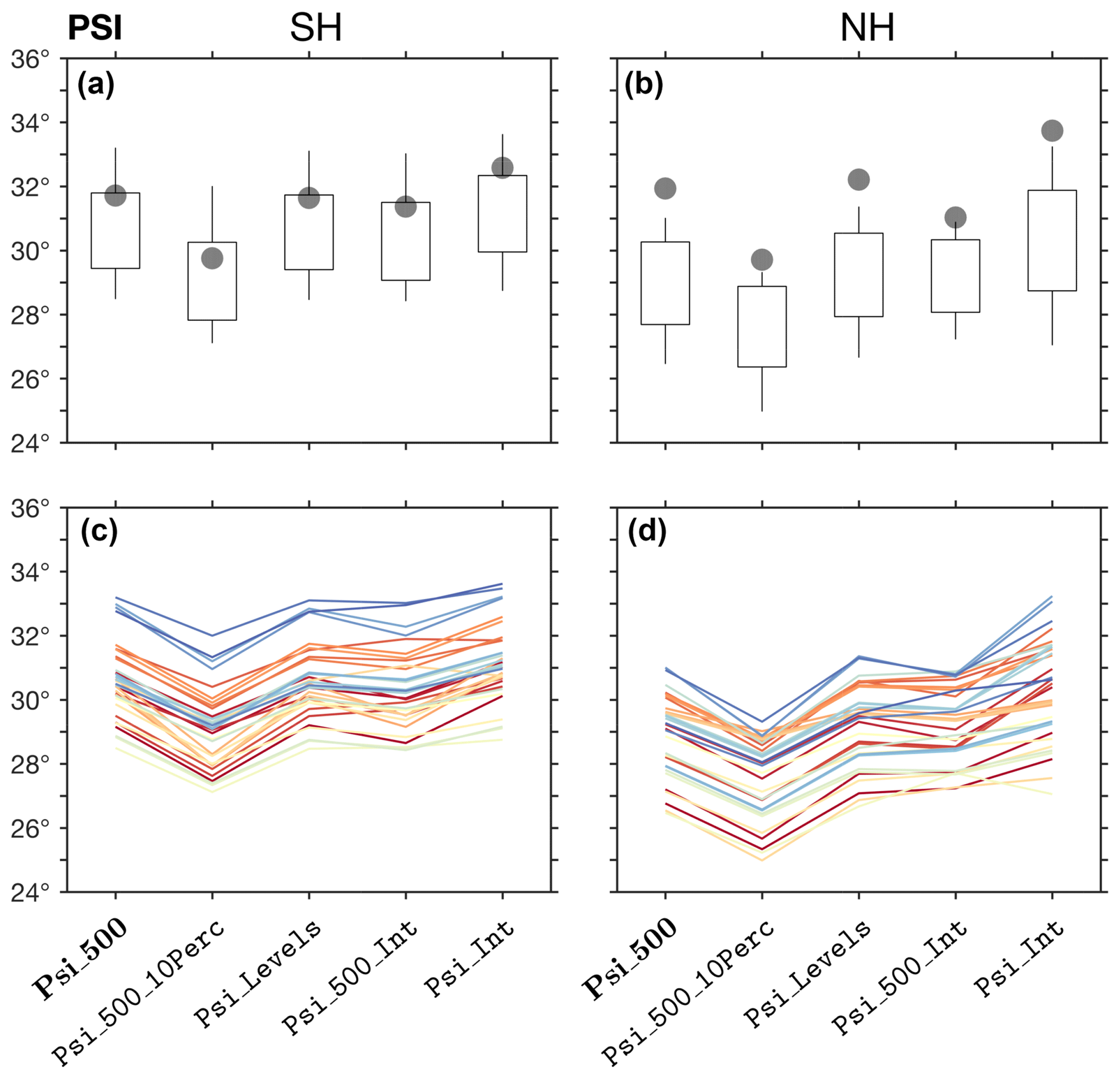
Figure 12The mean latitude for the five available PSI metric methods, derived
from annual means of the zonal-mean meridional wind in the SH (a, c)
and NH (b , d), for the period 1979–2004. The default method
(Psi_500) is bolded. Positive values are used for both the NH and
SH. In panels (a) and (b), candle boxes show mean ±1
standard deviation of CMIP5 inter-model spread; candle wicks show maximal and
minimal CMIP5 model values. ERAI values are shown in gray dots. In panels
(c) and (d), values for each model are shown in different
colors. The input parameter Lat_Uncertainty is set to zero
(default) in all of the methods.
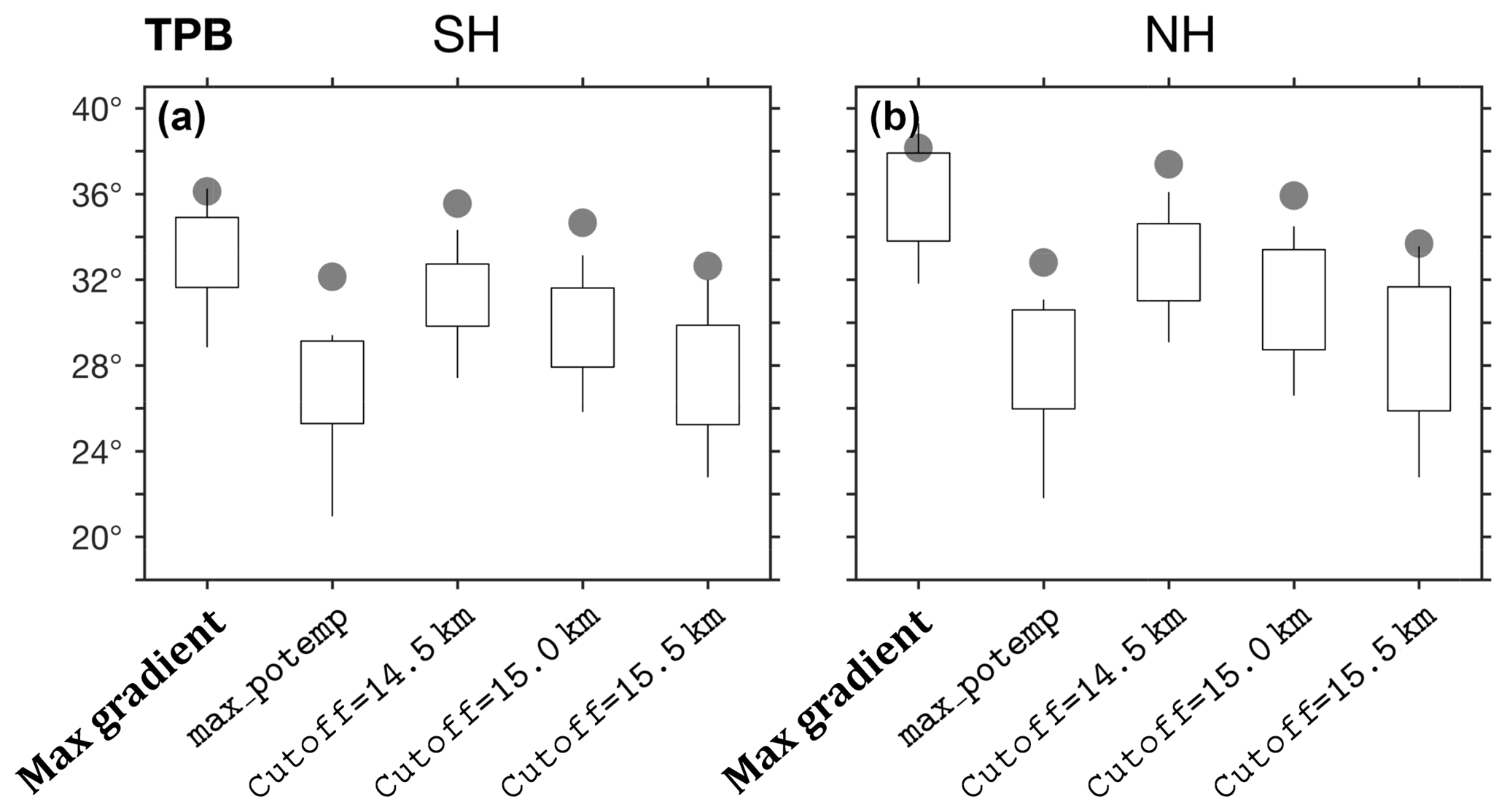
Figure 13The mean latitude for the max_gradient,
max_potemp, and cutoff methods of the TPB metric, as in
Fig. 12a, b. For the cutoff method, geopotential height
cutoff values of 14 500, 15 000 (default), and 15 500 m are shown. For
Cutoff=15 500 and for max_potemp, three of the models
produced unrealistic results and were removed from the analysis.
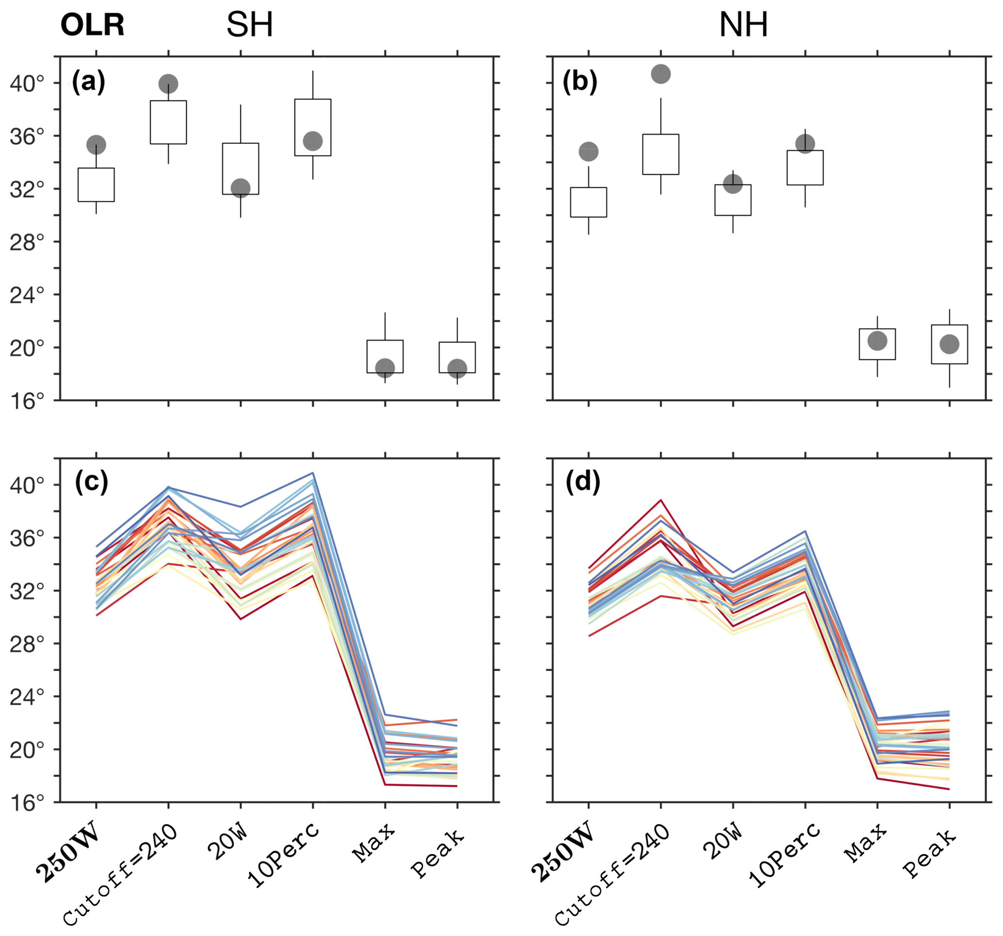
Figure 14As in Fig. 12 for the OLR metric methods 250W,
cutoff (with Cutoff=240), 20W, 10Perc,
max, and peak.
To demonstrate the sensitivity of the various methods to the smoothing
parameter n, the sensitivity of the STJ:core and
STJ:adjusted methods, and of the TPB:max_gradient and
TPB:max_potemp methods to n is analyzed in Figs. 9
and 10. Additional information on the sensitivity to n of the
interannual variability and decadal trends in these metrics is provided in
the Supplement (Figs. S1–S4). Consistent with Fig. 3, inter-model
spread generally increases with n for STJ:core, presumably
due to increased sensitivity to noise, but not for STJ:adjusted. The
standard deviation of inter-model spread is also significantly greater in the
SH for STJ:core (greater than 8∘ for n >10;
Fig. 9a) compared with STJ:adjusted (∼2∘ for
n ≥6) but is approximately the same for both methods in the
NH (∼4∘ for n ≥6; Fig. 9b, d). This
suggests that the differences between the two methods in the SH are due to
the stronger signal of the midlatitude jet in the SH, which is successfully
removed in the STJ:adjusted method (Fig. 6).
Due to the sharp gradient in the tropopause height at the tropopause break
(Fig. 4), the mean position of the TPB:max_gradient
method (which identifies the latitude of maximal meridional gradient;
Sect. 3.2) is insensitive to the smoothing parameter in both hemispheres for
n ≥6 (Fig. 10a, b). However, the inter-model spread in
interannual variability and decadal trends generally increases with
n (Fig. S3). Therefore, the default smoothing parameter for this
method is set to n=6 (i.e., the max method). In contrast,
the TPB:max_potemp method (which identifies the latitude of maximal
difference in the potential temperature between the tropopause and the
surface; Sect. 3.2) is insensitive to the smoothing parameter for
n ≥20 (Figs. 10c–d, S4). The default smoothing
parameter for this method is therefore set to n=30 (i.e., the
peak method). Likewise, since for most of the metrics the optimal
smoothing level is not known, to reduce method dependence on external
parameters, the peak method (i.e., weak smoothing) is preferred as
the default method for finding the latitude of the maximum.
4.4 Inter-method analysis
The mean values of the default methods in each of the eight metrics implemented in TropD are shown in Fig. 11. For simplicity, our inter-method analysis focuses on the mean values of the various metrics, derived from annual means, for the period 1979–2004. Additional method sensitivity analysis for the interannual variability and the decadal trends of the eight metrics is provided in the Supplement (Figs. S5–S9).
Figure 12 shows the five available methods of the PSI metric derived
from annual-mean values of the zonal-mean meridional wind. The five PSI
methods vary consistently across models (Fig. 12c, d). In addition,
the differences between the five PSI methods per model
( on average) are generally
smaller than the inter-model spread ( standard deviation). Therefore, given the prevalence of the
Psi_500 method in studies of the tropical width, this method is set
as the default method for the PSI metric in TropD.
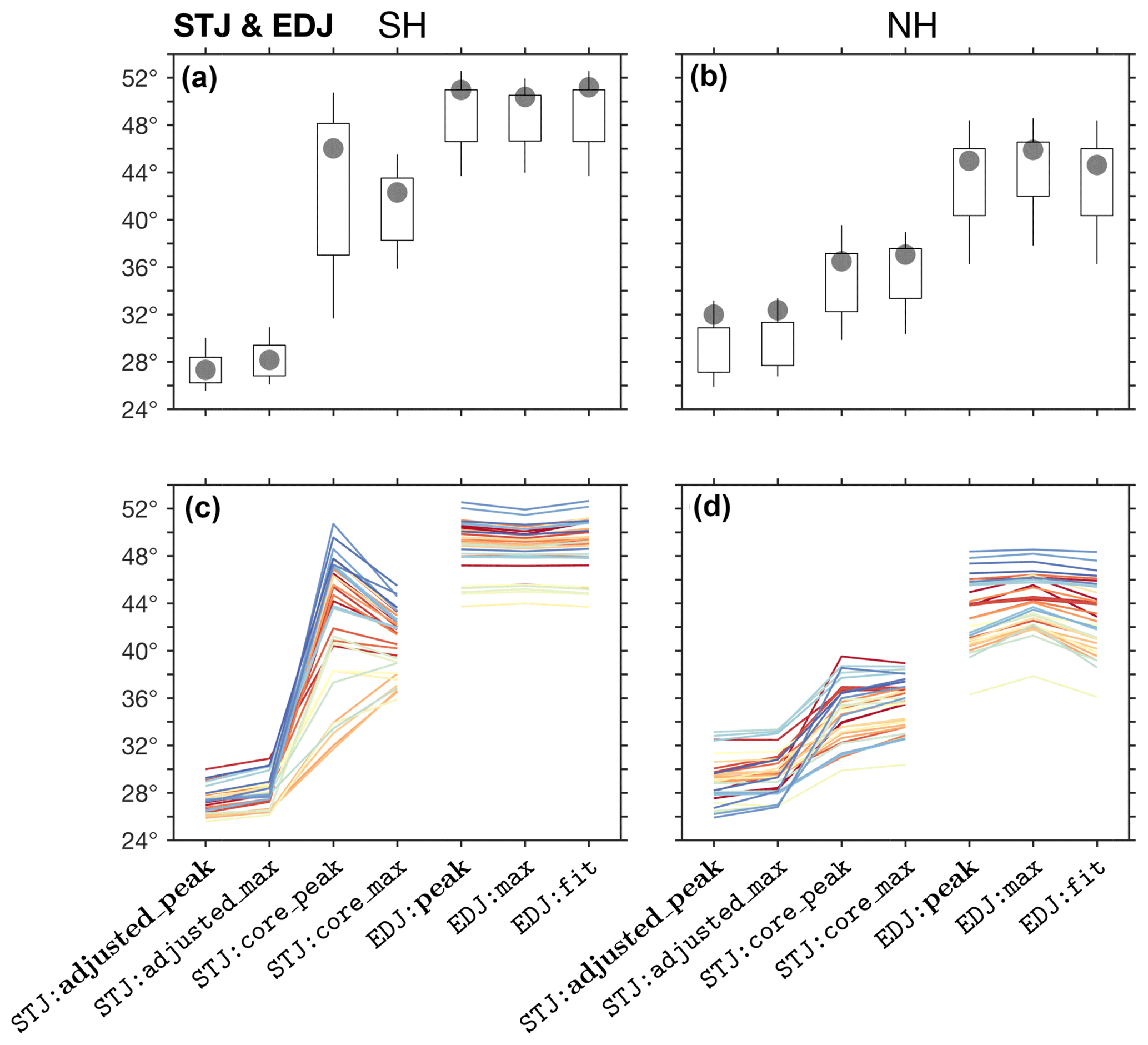
Similar candle plots for the TPB and OLR metrics are shown in Figs. 13 and 14, for the STJ and EDJ metrics in Fig. 15, and for the PE, UAS, and PSL metrics in Fig. 16. As for the PSI metric, the default method for each metric is shown in bolded text. CMIP5 models generally underestimate mean metric values, interannual variability, and trend in both PSI and TPB metrics when compared with ERAI (Figs. 12, 13, S5, and S6), but are generally consistent with ERAI values for the other metrics (Figs. 14–16, S7–S9). As reported in previous studies, inconsistencies between reanalyses and models during this period are attributable to internal variability, variations in the response to anthropogenic forcing, and the unknown reliability of the reanalyses (e.g., Adam et al., 2014; Garfinkel et al., 2015; Mantsis et al., 2017). However, for all of the metrics, the relative variations between the methods in both ERAI and the CMIP5 models are generally the same. This reinforces our assertion that uncertainty in analyses of tropical width variations can be reduced by applying consistent methodologies across datasets.
Figure 4 shows the tropopause height and the difference in the
potential temperature between the tropopause and the surface during the
decades beginning in 1979 and 1995. Consistent with theory in a warming
climate (e.g., Levine and Schneider, 2015), both the tropopause height and the
potential temperature difference increase in the tropics during 1979–2004.
However, the changes in the tropopause height near the tropopause break
differ substantially between hemispheres, while the change in the potential
temperature difference is uniform across the tropics. These qualitative
differences in the profiles of the tropopause height and the potential
temperature account for the differences in the TPB:max_gradient and
TPB:max_potemp methods (Figs. 13, S3–S4, S6) and may lead
to differing estimates of tropical width variations. In addition, the mean
value, interannual variability, and decadal trends of the TPB:cutoff
method are sensitive to the cutoff parameter (Figs. 13, S6). The
variance across models generally increases as the cutoff value nears the
maximal value of the tropopause height (∼16 km) in the tropics, which
goes along with reduced meridional gradients of the tropopause and hence
increased sensitivity to the cutoff parameter. Due to its simplicity and its
direct association with the tropopause height, max_gradient is set
as the default method for the TPB metric.
A similar sensitivity to subjective cutoff parameters is seen in the OLR
metric (i.e., the cutoff, 20W, and 10Perc methods;
Figs. 14, S7). Due to uncertainty in observations, the reliability of
the zonal-mean OLR in CMIP5 models is poorly known (e.g.,
Fig. 5; Stephens et al., 2012), but OLR anomalies in CMIP5 models are
generally well correlated with observations (Smith et al., 2015). However, given
the strong sensitivity of the OLR metric to subjective cutoff parameters, and
since decadal changes in OLR are generally smaller than the inter-model
spread, estimates of recent tropical widening using this metric are highly
uncertain (Davis and Rosenlof, 2012; Waugh et al., 2018). The 250W method, which is the
most commonly used OLR metric (e.g., Hu and Fu, 2007; Johanson and Fu, 2009; Davis and Rosenlof, 2012), is
set as the default OLR method.
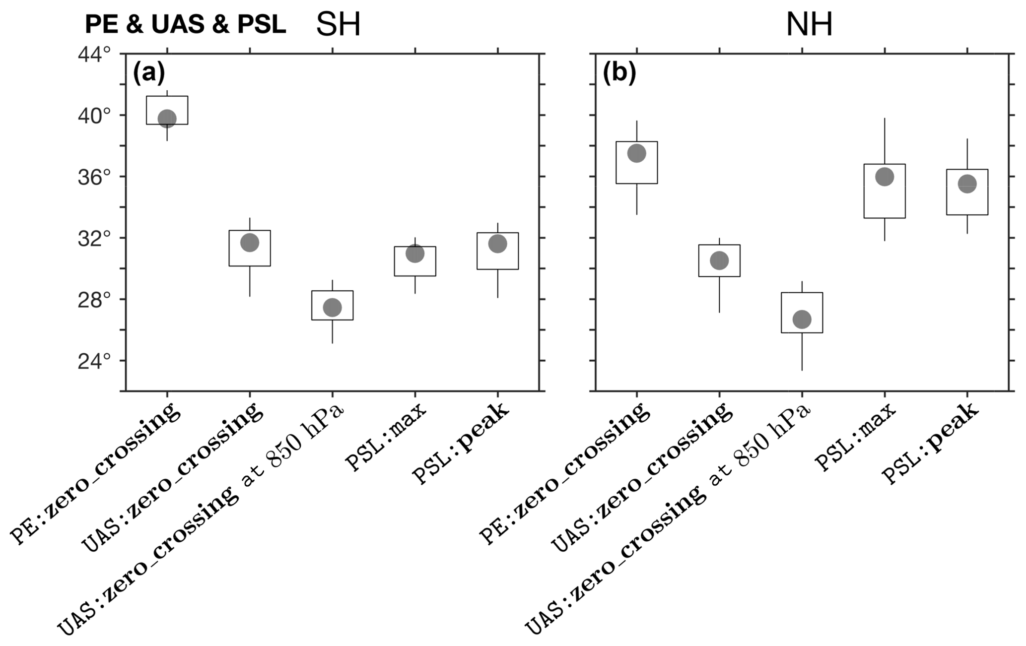
Figure 16As in Fig. 12a, b for PE:zero_crossing,
UAS:zero_crossing using the zonal wind both at the surface and at
the 850 hPa level, PSL:max, and PSL:peak.
The subtraction of the 850 hPa wind from the upper-level zonal wind
distinguishes the signal of the subtropical jet from that of the eddy-driven
jet (Fig. 6; Davis and Birner, 2016), accounting for the strong
differences between the STJ:core and STJ:adjusted methods
(Fig. 15). In addition, since below the STJ the surface zonal wind is
expected to vanish, the subtraction of near-surface wind is not expected to
strongly affect the signal of the STJ near the edge of the Hadley
circulation. Since, in addition, the subtraction of the 850 hPa wind reduces
inter-model spread (Figs. 6, 15), the adjusted_peak
method is set as the default method for the STJ metric. As mentioned above,
because the optimal smoothing level is not known, the peak method is
set as the default method for finding the latitude of the maximum for both
the STJ and EDJ metrics.
The subtropical meridional profiles of the upper- and lower-level zonal wind
(Fig. 6) and the sea-level pressure (Fig. 7c) are
significantly more flat in the NH relative to the SH, making the STJ, EDJ,
and PSL metrics more sensitive to noise in the NH. Therefore, using different
smoothing levels for the SH and NH metrics may be advisable in some cases
(e.g., using max in the NH and peak in the SH, as
in Waugh et al., 2018). Similarly, due to continental effects, variance near the
surface in the NH subtropics is generally greater than in the SH. This can
lead to differences between hemispheres when the zero-crossing uniqueness
criteria are used (e.g., Fig. 8). Therefore, using different values of
the Lat_Uncertainty parameter for NH and SH metrics may be
advisable in some cases for the near-surface metrics UAS and PE, as well as
for PSI. For the UAS metric, the above holds even when the input wind is the
zonal wind at the 850 hPa level (Fig. 6), which produces more
equatorward UAS metric values, but varies consistently across models with UAS
values derived from the surface wind (Fig. 16).
The TropD software package provides methodologies for eight commonly used metrics of the tropical width. TropD is designed to reduce, or aid in the assessment of, the methodological component of the uncertainty in studies of tropical width variations by
-
compiling the relevant methods for each metric category;
-
reducing all of the calculations in the metric methods to two basic operations: (i) finding the latitude of the zero crossing or (ii) finding the latitude of the maximum;
-
providing functions for calculating the meridional mass stream function and the tropopause height according to generally accepted guidelines;
-
providing consistent methods for implementing threshold criteria;
-
using consistent smoothing across methods; and
-
using consistent meridional limits for the various metrics.
In addition, TropD allows flexibility in the input parameters (e.g., in the cutoff and smoothing parameters) which enables consistent sensitivity testing of the metrics in various datasets, as well as testing new methods.
Our method sensitivity analysis highlights the importance of differentiating between variations which arise from parameter choices and inconsistent resolutions across datasets, as opposed to differences which arise from the representation of physical processes in the datasets. The analysis suggests that careful use of the metric methods can reduce some of the spurious uncertainty. For example, using different metric methods for each hemisphere can minimize the spurious uncertainty seen in inter-model variations of the surface metrics (Fig. 16) and the grid sensitivity of the EDJ metric (Table 2). Similarly, spurious uncertainty can be significantly reduced by proper method selection, which can minimize undesired effects such as temporal averaging biases, grid dependence, sensitivity to noise, and sensitivity to threshold criteria.
Based on our inter-method analysis, the default methods and parameters for each metric category are optimized for the present climate. Nevertheless, the TropD code can be easily adapted for studies of past climates or perturbations of the present climate, which, as in studies of recent tropical width variations, suffer from unknown spurious uncertainty. Similarly, elements of the TropD code can be applied to a wide range of studies beyond calculations of the tropical width (e.g., the position of the intertropical convergence zone, tropopause height variations, and circulation intensity variations) where the use of standardized methodology can reduce spurious uncertainty.
The TropD (MATLAB) software, reference precalculated metrics, and reference fields are freely available at http://www.oriadam.info (last access: 1 October 2018) or via http://www.zenodo.org (last access: 3 September 2018), https://doi.org/10.5281/zenodo.1157043 (Adam, 2018). TropD is free for non-commercial use. The PyTropD software is available via GitHub https://tropd.github.io/pytropd/index.html (last access: 6 September 2018).
The supplement related to this article is available online at: https://doi.org/10.5194/gmd-11-4339-2018-supplement.
The text was written by OA with suggestions and editorial contributions from all of the co-authors. The MATLAB code was written by OA with algorithmic contributions from all of the co-authors. The Python code was translated from MATLAB by AM with help from PS and the TropD team.
The authors declare that they have no conflict of interest.
This work is part of the collaborative efforts of the International Space
Science Institute (ISSI) Tropical Width Diagnostics Intercomparison Project
and the US Climate Variability and Predictability Program (US CLIVAR)
Changing Width of the Tropical Belt Working Group. The authors thank the
members of these groups as well as the ISSI and US CLIVAR offices and
sponsoring agencies (ESA, Swiss Confederation, Swiss Academy of Sciences,
University of Bern, NASA, NOAA, NSF, and DOE) for their support. We
acknowledge the World Climate Research Programme's Working Group on Coupled
Modelling, which is responsible for CMIP, and we thank the climate modeling
groups for producing and making available their model output. Ori Adam
acknowledges support by the Israeli Science Foundation grant 1185/17. Alison
Ming acknowledges funding from the NERC standard grant code
NE/N011813/1.
Edited by: Juan Antonio Añel
Reviewed by: two anonymous referees
Adam, O.: TropD: Tropical width diagnostics software package (Version 1.3), Zenodo, https://doi.org/10.5281/zenodo.1413330, 2018. a
Adam, O., Schneider, T., and Harnik, N.: Role of changes in mean temperatures versus temperature gradients in the recent widening of the Hadley circulation, J. Climate, 27, 7450–7461, 2014. a
Adam, O., Bischoff, T., and Schneider, T.: Seasonal and interannual variations of the energy flux equator and ITCZ, Part I: Zonally averaged ITCZ position, J. Climate, 29, 3219–3230, https://doi.org/10.1175/JCLI-D-15-0512.1, 2016. a
Archer, C. L. and Caldeira, K.: Historical trends in the jet streams, Geophys. Res. Lett., 35, L08803, https://doi.org/10.1029/2008GL033614, 2008. a, b
Birner, T.: Recent widening of the tropical belt from global tropopause statistics: Sensitivities, J. Geophys. Res., 115, D23109, https://doi.org/10.1029/2010JD014664, 2010. a, b, c, d
Choi, J., Son, S.-W., Lu, J., and Min, S.-K.: Further observational evidence of Hadley cell widening in the Southern Hemisphere, Geophys. Res. Lett., 41, 2590–2597, https://doi.org/10.1002/2014GL059426, 2014. a, b, c
D'Agostino, R., Lionello, P., Adam, O., and Schneider, T.: Factors controlling Hadley circulation changes from the Last Glacial Maximum to the end of the 21st century, Geophys. Res. Lett., 44, 8585–8591, https://doi.org/10.1002/2017GL074533, 2017. a
Davis, N. and Birner, T.: Seasonal to multidecadal variability of the width of the tropical belt., J. Geophys. Res.-Atmos., 118, 7773–7787, https://doi.org/10.1002/jgrd.50610, 2013. a
Davis, N. and Birner, T.: Climate Model Biases in the Width of the Tropical Belt, J. Climate, 29, 1935–1954, https://doi.org/10.1175/JCLI-D-15-0336.1, 2016. a, b, c
Davis, N. and Birner, T.: On the Discrepancies in Tropical Belt Expansion between Reanalyses and Climate Models and among Tropical Belt Width Metrics, J. Climate, 30, 1211–1231, https://doi.org/10.1175/JCLI-D-16-0371.1, 2017. a, b, c, d, e, f, g, h, i
Davis, S., Hassler, B., and Rosenlof, K.: Revisiting ozone measurements as an indicator of tropical width, Progress in Earth and Planetary Science, 5, 56, https://doi.org/10.1186/s40645-018-0214-5, 2018. a
Davis, S. M. and Rosenlof, K. H.: A Multidiagnostic Intercomparison of Tropical-Width Time Series Using Reanalyses and Satellite Observations, J. Climate, 25, 1061–1078, https://doi.org/10.1175/JCLI-D-11-00127.1, 2012. a, b, c, d, e, f, g, h, i, j
Dee, D., Uppala, S. M., Simmons, A. J., Berrisford, P., Poli, P., Kobayashi, S., Andrae, U., Balmaseda, M., Balsamo, G., Bauer, P., Beljaars, A. C. M., van de Berg, L., Bidlot, J., Bormann, N., Delsol, C., Dragani, R., Fuentes, M., Geer, A., Haimberger, L., Healy, S., Hersbach, H., Holm, E., Isaksen, L., Kallberg, P., Kohler, M., Matricardi, M., McNally, A., Monge-Sanz, B., Morcrette, J.-J., Park, B.-K., Peubey, C., de Rosnay, P., Tavolato, C., Thepaut, J.-N., and Vitart, F.: The ERA-Interim reanalysis: configuration and performance of the data assimilation system, Q. J. Roy. Meteor. Soc., 137, 553–597, 2011. a
Garfinkel, C., Waugh, D., and Polvani, L.: Recent Hadley cell expansion: the role of internal atmospheric variability in reconciling modeled and observed trend, Geophys. Res. Lett., 42, 10824–10831, https://doi.org/10.1002/2015GL066942, 2015. a
Held, I. M.: The General Circulation of the Atmosphere, in: Proc. Program in Geophysical Fluid Dynamics, Woods Hole Oceanographic Institution, Woods Hole, MA, 2000. a
Hu, Y. and Fu, Q.: Observed poleward expansion of the Hadley circulation since 1979, Atmos. Chem. Phys., 7, 5229–5236, https://doi.org/10.5194/acp-7-5229-2007, 2007. a, b, c, d
Hu, Y., Zhou, C., and Liu, J.: Observational evidence for the poleward expansion of the Hadley circulation, Adv. Atmos. Sci., 28, 33–44, 2011. a, b
Hudson, R. D., Andrade, M. F., Follette, M. B., and Frolov, A. D.: The total ozone field separated into meteorological regimes – Part II: Northern Hemisphere mid-latitude total ozone trends, Atmos. Chem. Phys., 6, 5183–5191, https://doi.org/10.5194/acp-6-5183-2006, 2006. a
Johanson, C. M. and Fu, Q.: Hadley Cell Widening: Model Simulations versus Observations, J. Climate, 22, 2713–2725, 2009. a, b
Kang, S. M. and Polvani, L. M.: The interannual relationship between the eddy-driven jet and the edge of the Hadley cell, J. Climate, 24, 563–568, 2011. a, b
Kidston, J. and Gerber, E. P.: Intermodel variability of the poleward shift of the austral jet stream in the CMIP3 integrations linked to biases in 20th century climatology, Geophys. Res. Lett., 37, L09708, https://doi.org/10.1029/2010GL042873, 2010. a
Kim, H. K. and Lee, S. Y.: Hadley Cell Dynamics in a Primitive Equation Model. Part II: Nonaxisymmetric Flow, J. Atmos. Sci., 58, 2859–2871, 2001. a
Korty, R. L. and Schneider, T.: Extent of Hadley circulations in dry atmospheres, Geophys. Res. Lett., 35, L23803, https://doi.org/10.1029/2008GL035847, 2008. a
Levine, X. and Schneider, T.: Baroclinic Eddies and the Extent of the Hadley Circulation: An Idealized GCM Study, J. Atmos. Sci., 72, 2744–2761, https://doi.org/10.1175/JAS-D-14-0152.1, 2015. a, b
Levine, X. J. and Schneider, T.: Response of the Hadley Circulation to Climate Change in an Aquaplanet GCM Coupled to a Simple Representation of Ocean Heat Transport, J. Atmos. Sci., 68, 769–783, 2011. a
Liebmann, B. and Smith, C.: Description of a Complete (Interpolated) Outgoing Longwave Radiation Dataset, B. Am. Meteorol. Soc., 77, 1275–1277, 1996. a
Lu, J., Vecchi, G. A., and Reichler, T.: Expansion of the Hadley cell under global warming, Geophys. Res. Lett., 34, L06805, https://doi.org/10.1029/2006GL028443, 2007. a, b
Mantsis, D., Sherwood, S., Allen, R., and Shi, L.: Natural variations of tropical width and recent trends, Geophys. Res. Lett., 44, 3825–3832, https://doi.org/10.1002/2016GL072097, 2017. a
Reichler, T., Dameris, M., and Sausen, R.: Determining the tropopause height from gridded data, Geophys. Res. Lett., 30, 2042, https://doi.org/10.1029/2003GL018240, 2003. a
Schneider, T.: The General Circulation of the Atmosphere, Ann. Rev. Earth Pl. Sc., 34, 655–688, 2006. a, b
Seidel, D. J. and Randel, W. J.: Recent widening of the tropical belt: Evidence from tropopause observations, J. Geophys. Res., 112, D20113, https://doi.org/10.1029/2007JD008861, 2007. a, b
Smith, D. M., Allan, R. P., Coward, A. C., Eade, R., Hyder, P., Liu, C., Loeb, N. G., Palmer, M. D., Roberts, C. D., and Scaife, A. A.: Earth's energy imbalance since 1960 in observations and CMIP5 models, Geophys. Res. Lett., 42, 1205–1213, https://doi.org/10.1002/2014GL062669, 2015. a
Solomon, A., Polvani, L. M., Waugh, D. W., and Davis, S. M.: Contrasting upper and lower atmospheric metrics of tropical expansion in the Southern Hemisphere, Geophys. Res. Lett., 43, 10496–10503, https://doi.org/10.1002/2016GL070917, 2016. a, b, c, d
Stephens, G. L., Li, J., Wild, M., Clayson, C. A., Loeb, N., Kato, S., L'Ecuyer Jr., T., P. W. S., Lebsock, M., and Andrews, T.: An update on Earth's energy balance in light of the latest global observations, Nat. Geosci., 5, 691–696, https://doi.org/10.1038/ngeo1580, 2012. a
Waugh, D., Grise, K. M., Seviour, W., Davis, S., Davis, N., Adam, O., Son, S.-W., and Simpson, I. R.: Revisiting the Relationship among Metrics of Tropical Expansion, J. Climate, 31, 7565–7581, https://doi.org/10.1175/JCLI-D-18-0108.1, 2018. a, b, c, d, e
WMO: Meteorology – A three-dimensional science, WMO Bull., 6, 134–138, 1957. a
Woollings, T., Hannachi, A., and Hoskins, B.: Variability of the North Atlantic eddy-driven jet stream, Q. J. Roy. Meteorol. Soc., 136, 856–868, https://doi.org/10.1002/qj.625, 2010. a