the Creative Commons Attribution 4.0 License.
the Creative Commons Attribution 4.0 License.
 | 16 Nov 2018
Global simulation of tropospheric chemistry at 12.5 km resolution: performance and evaluation of the GEOS-Chem chemical module (v10-1) within the NASA GEOS Earth system model (GEOS-5 ESM)
Christoph A. Keller
Michael S. Long
Tomás Sherwen
Benjamin Auer
Arlindo Da Silva
Jon E. Nielsen
Steven Pawson
Matthew A. Thompson
Atanas L. Trayanov
Katherine R. Travis
Stuart K. Grange
Mat J. Evans
Daniel J. Jacob
We present a full-year online global simulation of tropospheric chemistry (158 coupled species) at cubed-sphere c720 () resolution in the NASA Goddard Earth Observing System Model version 5 Earth system model (GEOS-5 ESM) with GEOS-Chem as a chemical module (G5NR-chem). The GEOS-Chem module within GEOS uses the exact same code as the offline GEOS-Chem chemical transport model (CTM) developed by a large atmospheric chemistry research community. In this way, continual updates to the GEOS-Chem CTM by that community can be seamlessly passed on to the GEOS chemical module, which remains state of the science and referenceable to the latest version of GEOS-Chem. The 1-year G5NR-chem simulation was conducted to serve as the Nature Run for observing system simulation experiments (OSSEs) in support of the future geostationary satellite constellation for tropospheric chemistry. It required 31 wall-time days on 4707 compute cores with only 24 % of the time spent on the GEOS-Chem chemical module. Results from the GEOS-5 Nature Run with GEOS-Chem chemistry were shown to be consistent to the offline GEOS-Chem CTM and were further compared to global and regional observations. The simulation shows no significant global bias for tropospheric ozone relative to the Ozone Monitoring Instrument (OMI) satellite and is highly correlated with observations spatially and seasonally. It successfully captures the ozone vertical distributions measured by ozonesondes over different regions of the world, as well as observations for ozone and its precursors from the August–September 2013 Studies of Emissions, Atmospheric Composition, Clouds and Climate Coupling by Regional Surveys (SEAC4RS) aircraft campaign over the southeast US. It systematically overestimates surface ozone concentrations by 10 ppbv at sites in the US and Europe, a problem currently being addressed by the GEOS-Chem CTM community and from which the GEOS ESM will benefit through the seamless update of the online code.


Integration of atmospheric chemistry into Earth system models (ESMs) has been identified as a next frontier for ESM development (National Research Council, 2012) and is a priority science area for atmospheric chemistry research (National Academies of Sciences, Engineering, and Medicine, 2016). Atmospheric chemistry drives climate forcing and feedbacks, is an essential component of global biogeochemical cycling, and is key to air quality applications. A growing ensemble of atmospheric chemistry observations from space needs to be integrated into ESM-based data assimilation systems. Models of atmospheric chemistry are rapidly evolving, and an atmospheric chemistry module within an ESM must be able to readily update to the state of the science. We have developed such a capability by integrating the Goddard Earth Observing System with chemistry (GEOS-Chem) chemical transport model (CTM) as a comprehensive and seamlessly updatable atmospheric chemistry module in the NASA GEOS ESM (Long et al., 2015). Here, we present the first application and evaluation of this GEOS-Chem capability within GEOS version 5 (GEOS-5) for a full-year global simulation of tropospheric ozone chemistry at cubed-sphere c720 () resolution. This simulation is now serving as the Nature Run (pseudo-atmosphere) for observing system simulation experiments (OSSEs) in support of the near-future geostationary satellite constellation for tropospheric chemistry (Zoogman et al., 2017).
GEOS-Chem (http://geos-chem.org) is an open-source global 3-D Eulerian model of atmospheric chemistry driven by GEOS-5 assimilated meteorological data. It includes state-of-the-science capabilities for tropospheric and stratospheric gas–aerosol chemistry (Eastham et al., 2014; Hu et al., 2017), with additional capabilities for aerosol microphysics (Trivitayanurak et al., 2008; Yu and Luo, 2009). It is used by over a hundred active research groups in 25 countries around the world for a wide range of atmospheric chemistry applications, providing a continual stream of innovation (Hu et al., 2017). Strong version control and benchmarking maintain the integrity and referenceability of the model. The code is freely available through an open license (http://acmg.seas.harvard.edu/geos/geos_licensing.html, last access: 14 September 2018).
GEOS-Chem as used by the atmospheric chemistry community operates in an “offline” CTM mode, without explicit simulation of meteorology. Meteorological data are inputted to the model to simulate chemical transport and other processes. The offline approach makes the model simple to use and facilitates community development of the core chemical module that describes local chemical sources and sinks from emissions, reactions, thermodynamics, and deposition. Implementing the GEOS-Chem chemical module into ESMs offers a state-of-the-science and referenceable representation of atmospheric chemistry, but it is essential that the module be able to automatically incorporate new updates as the offline model evolves. Otherwise, it would become quickly dated and unsupported.
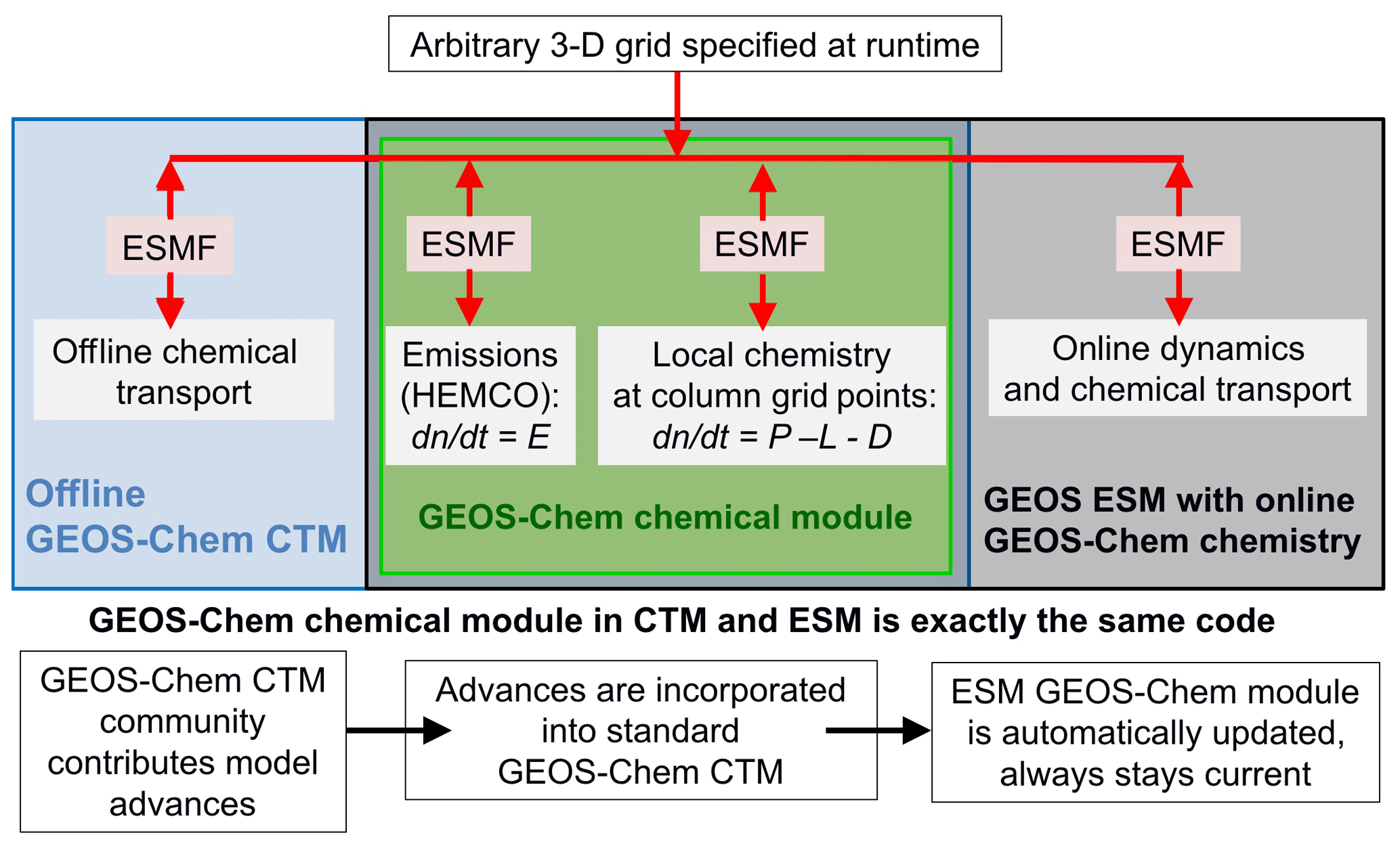
Figure 1Schematic of GEOS-Chem chemical module used either offline as a chemical transport model (CTM) or online in an Earth system model (ESM), with interfaces managed through the Earth system modeling framework (ESMF). The module is grid independent, with individual computations done on atmospheric columns at user-selected grid points. It computes local changes in concentrations with time (dn∕dt) as a result of emissions (E), chemical production (P), chemical loss (L), and deposition (D). Emissions are handled through the Harvard-NASA EMission COmponent (HEMCO) to provide ESM users the option of only integrating emissions.
From a GEOS-Chem atmospheric chemistry user perspective, there are a number of reasons why an online simulation capability is of interest. Users working on both climate and atmospheric chemistry modeling can use the same module for both, thus improving the consistency of their approach. Some atmospheric chemistry problems involving fast coupling between chemistry and dynamics, such as aerosol–cloud interactions, require online coupling. As the resolution of ESMs increases, use of archived meteorological data becomes more difficult and incurs increased error (Yu et al., 2018), so online simulation can become more attractive. Finally, online simulations can take advantage of vast computational resources available at climate modeling centers to achieve very high resolution as illustrated in this paper. Such high-resolution model outputs are particularly important for air quality and human health applications (Cohen et al., 2017) and for OSSEs to support the design of satellite missions (Barré et al., 2016; Claeyman et al., 2011; Fishman et al., 2012; Yumimoto, 2013; Zoogman et al., 2014). A future modus operandi for the GEOS-Chem community might involve development in the offline model at coarse resolution, and online simulations when high resolution is required.
We have developed the capability to efficiently integrate the GEOS-Chem chemical module into ESMs in a way that enables seamless updating to the latest standard version of GEOS-Chem. This involved transformation of GEOS-Chem into a grid-independent and Earth system modeling framework (ESMF)-compliant model (Long et al., 2015). The exact same code is now used in stand-alone offline mode (CTM) by the GEOS-Chem community and as an online chemical module within GEOS-5 (Fig. 1). Using the exact same code for both applications ensures that the chemical module in the ESM keeps current with the latest well-documented standard version of GEOS-Chem. An important component is the Harvard-NASA EMission COmponent (Keller et al., 2014), which allows GEOS-Chem users to build customized layers of emission inventories on any grid and with no editing of the GEOS-Chem source code. HEMCO is now the standard emission module in GEOS-Chem and is used in GEOS-5 as an independent module for applications when full chemistry is not needed.
Here, we apply the GEOS-Chem chemical module within GEOS-5 in a very-high-resolution (VHR) simulation of global tropospheric ozone chemistry. The simulation is conducted for 1 full year (2013–2014) at c720 cubed-sphere resolution () with 158 coupled chemical species. To the best of our knowledge, such a resolution in a state-of-the-science global simulation of tropospheric chemistry is unprecedented. Resolution not only increases the quality of local information, e.g., for air quality, but it also provides better representation of chemical non-linearities. We compare the model outputs with coarse offline GEOS-Chem CTM results and with independent observations for tropospheric ozone and precursors as a test of fidelity and increased power. We refer to this VHR simulation as the GEOS-5 Nature Run with GEOS-Chem chemistry, or G5NR-chem.
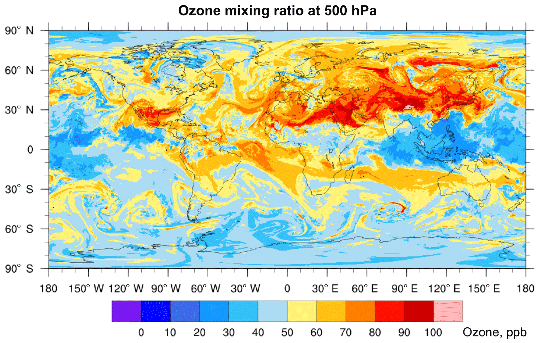
Figure 2The 500 hPa ozone distribution on 1 August 2013 at 00:00 Z simulated by GEOS-5 with the GEOS-Chem chemical module at cubed-sphere c720 () resolution.
An Eulerian (fixed frame of reference) CTM such as GEOS-Chem solves the system of coupled continuity equations for an ensemble of m species with number density vector :
where U is the wind vector including subgrid components to be parameterized as turbulent diffusion or convection. (Pi−Li)(n), Ei, and Di are the local chemical production and loss, emission, and deposition rates, respectively, of species i. Coupling across species is through the chemical term (Pi−Li). In GEOS-Chem, as in all 3-D CTMs, Eq. (1) is solved by operator splitting to separate the transport and local components over finite time steps. The local operator,
includes no transport terms (no spatial coupling) and thus reduces to a system of coupled ordinary differential equations (ODEs). It is commonly called the chemical operator even though emission and deposition terms are included. The transport operator,
does not involve coupling between chemical species.
Use of GEOS-Chem as chemical module in an ESM requires only the code that updates concentrations over a given time step for local production and loss as given by Eq. (2) (Fig. 1). The CTM has its own transport modules to solve Eq. (3) using archived meteorological inputs (offline), but these are not needed in the ESM where transport is computed as part of atmospheric dynamics (online).
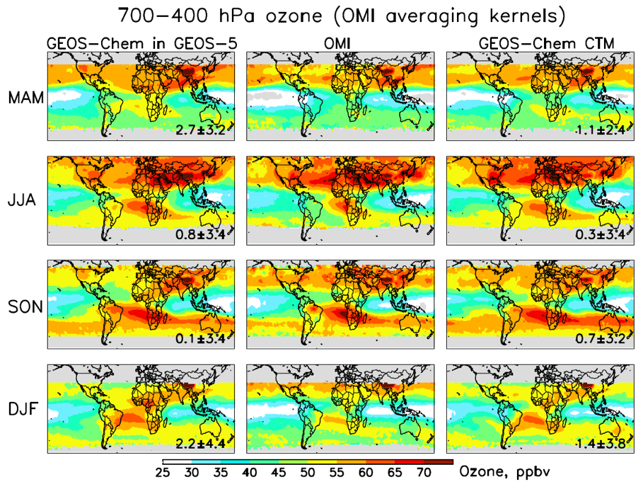
Figure 3Middle tropospheric ozone distribution at 700–400 hPa from the GEOS-5 Nature Run with GEOS-Chem chemistry (a), Ozone Monitoring Instrument (OMI) satellite observations (b), and the offline GEOS-Chem CTM (c) for four seasons covering July 2013–June 2014. The data are on a grid. All data are smoothed by the OMI averaging kernels, using a single fixed a priori profile so that variability is solely driven by observations. The OMI observations have been further corrected for a global mean positive bias of 3.6 ppbv (Hu et al., 2017). Both models are sampled along the OMI tracks. Numbers in the left and right columns are the mean model bias ± standard deviation. Gray shading indicates regions where OMI data are unreliable and not used (poleward of 45∘ in winter–spring and poleward of 60∘ year round; see Hu et al., 2017).
The ESM chemical module is tasked with updating chemical concentrations by integration of Eq. (2) on the ESM grid and time step. Exchange of information between the chemical module and other ESM modules can be done by various couplers such as ESMF (Hill et al., 2004). Our guiding principle is that the CTM and the ESM chemical module share the exact same code. This required restructuring GEOS-Chem to a grid-independent form and making the code compliant with the ESMF Modeling Analysis and Prediction Layer (MAPL) coupler used by GEOS (Long et al., 2015). The 1-D vertical columns are the smallest efficient unit of computation for the chemical module because several operations are vertically coupled, including radiative transfer, vertically distributed emissions, wet scavenging, and particle settling. In the now grid-independent GEOS-Chem code, horizontal grid points are selected at runtime through the ESMF interface. The chemical and emission modules proceed to solve Eq. (2) on 1-D columns for the specified horizontal grid points (Fig. 1). We managed to carry out this major software transformation in GEOS-Chem in a way that was completely transparent to CTM users (Long et al., 2015). The exact same ESMF-compliant, grid-independent GEOS-Chem code is now used both in the stand-alone CTM and within GEOS. This enables seamless integration of future new GEOS-Chem scientific developments into the GEOS chemical module, which thus always remains current and referenced to the latest standard version of GEOS-Chem.
An important step in transforming GEOS-Chem to a grid-independent structure was to reconfigure the emission module. The emission module consists of multiple layers of databases and algorithms describing emissions for different species and regions, with scaling factors defining diurnal/weekly/seasonal/secular trends or dependences on environmental variables. The databases are on different grids and time stamps, and may add to or supersede each other as controlled by the user. The HEMCO module allows users to choose any combination of emission inventories in NetCDF format, on any grid and with any scaling factors, and apply them to any model grid specified at runtime (Keller et al., 2014). HEMCO provides a complete functional separation of emissions from transport, deposition, and chemistry in GEOS-Chem. The purpose of this separation is that the ESM may need emissions independently from atmospheric chemistry, for example, to simulate species such as CO2 and methane. HEMCO is thus configured as a stand-alone component in the ESM, accessed separately through the ESMF interface (Fig. 1).
Some care is needed when interfacing the GEOS-Chem chemical module with fast vertical transport processes in GEOS-5 involving boundary layer mixing (Lock et al., 2000; Louis et al., 1982) and deep convection with wet scavenging. Here, we apply boundary layer mixing at every time step in GEOS-5 with emissions and dry deposition updates from GEOS-Chem but before applying chemistry. This avoids anomalies in the lowest model layer when the timescale for boundary layer mixing is shorter than the time step for emissions. Deep convective transport of chemical species including scavenging in the updrafts is performed by the GEOS-Chem convection scheme driven by instantaneous diagnostic variables from the GEOS-5 convection component (Molod et al., 2015). This takes advantage of the gas and aerosol scavenging capability of the GEOS-Chem scheme (Amos et al., 2012; Liu et al., 2001). Radon-222 tracer simulation tests within GEOS-5 show that the GEOS-Chem convection scheme closely reproduces the GEOS-5 convective transport (Yu et al., 2018). As convection becomes increasingly resolved at higher model resolution, the GEOS-5 subgrid convection parameterization (Moorthi and Suarez, 1992) is invoked less frequently. As a consequence, an increasing fraction of the washout in GEOS-Chem becomes characterized as large scale, as opposed to convective. No attempts were made to offset the possible increase in washout efficiency that may arise from this.
We perform a year-long (1 July 2013 to 1 July 2014) GEOS-5 simulation with GEOS-Chem at cubed-sphere c720 () horizontal resolution and 72 vertical levels extending up to 0.01 hPa. For initialization, we use 12 months at c48 resolution () followed by 6 months at c720 resolution. Figure 2 shows a snapshot of the simulated 500 hPa ozone field, illustrating the fine detail enabled by the very high resolution.
3.1 General description
The GEOS-5 Nature Run with GEOS-Chem chemistry is performed with the Heracles version of GEOS-5 (tag “M2R12K-3_0_GCC”). The finite-volume dynamics is run in a non-hydrostatic mode with a heartbeat time of 300 s applied to the physics, chemical, and dynamics components. The simulation is forced by downscaled meteorological data from the lower-resolution Modern-Era Retrospective Analysis for Research and Applications version 2 (MERRA-2) reanalysis (Gelaro et al., 2017; Molod et al., 2015). The downscaling is performed by using the replay capability in GEOS, which adds a forcing term to the model equations, constraining them to a specific trajectory to simulate the 2013–2014 meteorological year (Orbe et al., 2017). Downscaling applications filter the replay increments so that only the larger scales of the flow are constrained, allowing scales finer than the analysis to evolve freely. In this simulation, a wave number of 60 was chosen as the cutoff. The simulation is performed in two segments, with the first with GEOS-Chem turned off (“regular replay”). The analysis increment produced during the first run segment is saved and reused in the subsequent run with GEOS-Chem turned on (“exact increment”). This two-segment process is computationally more efficient, as it avoids rewinding and checkpointing the model with full chemistry during the regular replay stage.
The chemical module is GEOS-Chem version v10-01 in tropospheric-only mode. It is run “passively” in G5NR-chem; thus, aerosols and trace gases do not influence the meteorology. It includes detailed HOx−NOx–VOC–ozone–BrOx–aerosol tropospheric chemistry with 158 species and 412 reactions, following Jet Propulsion Laboratory (JPL) and International Union of Pure and Applied Chemistry (IUPAC) recommendations for chemical kinetics (Sander et al., 2011) and updates for BrOx and isoprene chemistry (Mao et al., 2013; Parrella et al., 2012). The default GEOS-Chem bulk aerosol scheme is used to simulate major components for dust, sea salt, black carbon, organic carbon, sulfate, nitrate, and ammonium aerosols (Fairlie et al., 2007; Jaeglé et al., 2011; Kim et al., 2015; Park et al., 2004; Wang et al., 2014). The Fast-JX scheme with approximate randomized cloud overlap method and taking aerosol loading into account is used to calculate photolysis frequencies (Bian and Prather, 2002), as implemented by Mao et al. (2010). Linearized stratospheric chemistry is used (McLinden et al., 2000; Murray et al., 2012). The dry deposition calculation is based on a resistance-in-series model (Wesely, 1989), as implemented by Wang et al. (1998). Wet scavenging of aerosols and gases is as described by Liu et al. (2001) and Amos et al. (2012).
Emissions are calculated through HEMCO v1.1.008 (Keller et al., 2014). They are the default 2013–2014 emissions for GEOS-Chem (Hu et al., 2017), with a few modifications. Open fire emissions are from the Quick Fire Emissions Dataset (QFED) version 2.4-r6 (Darmenov and Da Silva, 2015). US NOx emissions follow Travis et al. (2016). Parameterizations for lightning NOx (Murray et al., 2012) and mineral dust aerosol emissions (Zender et al., 2003) have large dependencies on grid resolution and are scaled globally following general GEOS-Chem practice to annual totals of 6.5 TgN for lightning and 840 TgC for dust. No adjustments are made to emission of biogenic volatile organic compounds (VOCs) (Guenther et al., 2012; Hu et al., 2015b) and sea salt aerosol (Jaeglé et al., 2011), both of which agree with GEOS-Chem emissions within 15 %. GEOS-Chem uses in-plume chemistry of ship emissions (PARANOx) to account for the excessive dilution of ship exhaust plumes at coarse model resolution (Vinken et al., 2011); this was disabled in the VHR simulation given that the Nature Run resolution is fine enough to resolve the non-linear chemistry associated with ship plume emissions. A summary of the various emission sources used for the simulation is given in Table A2.
Table 1Global tropospheric burdens.
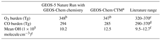
a Hu et al. (2017). b Calculated with a chemical tropopause as the 150 ppbv ozone isopleth. c Interquartile range of 50 models summarized in Young et al. (2018); limited observational estimates fall within that range. d Gaubert et al. (2016). e Global mean air-mass-weighted OH concentration. f From 16 model results summarized in Naik et al. (2013).
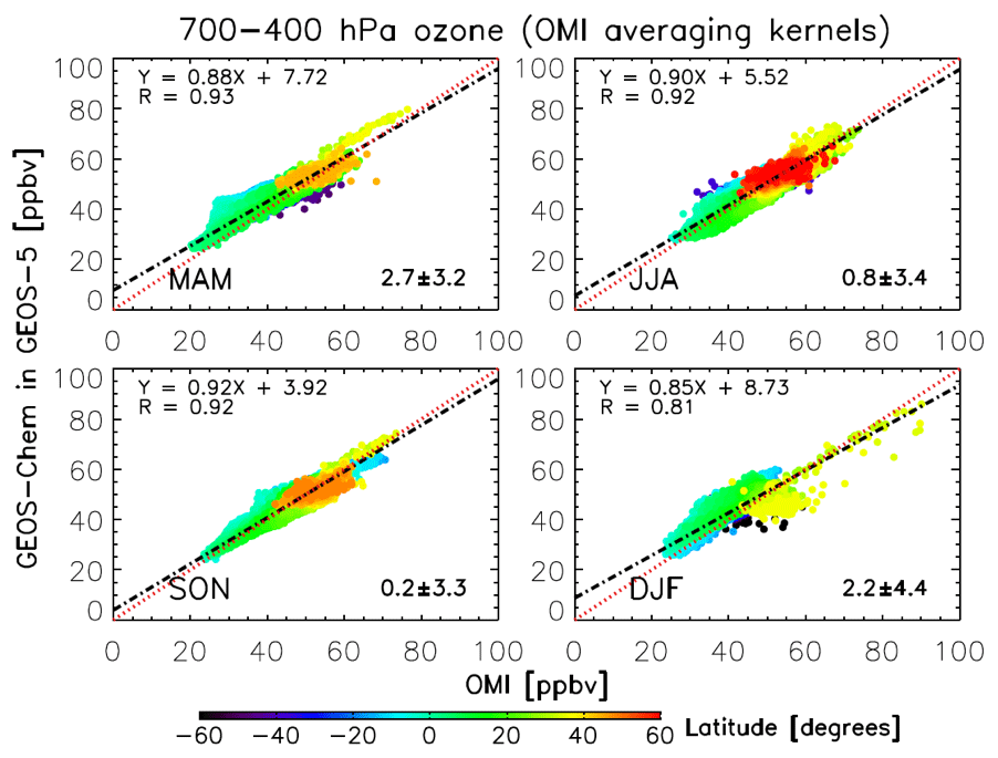
Figure 4Comparison of GEOS-5 Nature Run with GEOS-Chem chemistry to OMI 700–400 hPa ozone measurements for four seasons in July 2013–June 2014, colored by the latitude of the observations. Each point represents the seasonal mean for a grid cell. Black dashed lines show the best fit (reduced major axis regression) with regression parameters given in the inset. Numbers on the bottom right are the global mean model bias ± standard deviation. The 1:1 line is shown in red.
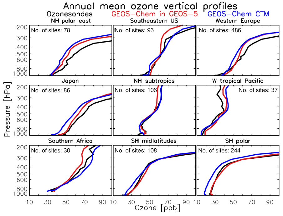
Figure 5Annual mean ozonesonde profiles in July 2013–June 2014 for representative global regions (Tilmes et al., 2012). Results from the GEOS-5 Nature Run with GEOS-Chem chemistry (red) are compared to observations (black) and to the GEOS-Chem CTM (blue; version in Hu et al., 2017). The models are sampled at the ozonesonde launch times and locations.
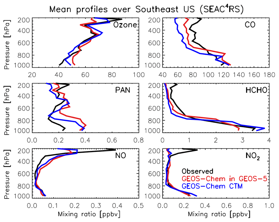
Figure 6Mean vertical profiles of trace gas concentrations over the southeast US during the NASA Studies of Emissions, Atmospheric Composition, Clouds and Climate Coupling by Regional Surveys (SEAC4RS) aircraft campaign (August–September 2013; Toon et al., 2016). Results from the GEOS-5 Nature Run with GEOS-Chem chemistry are compared to observations for ozone and NOx, CO, peroxyacetyl nitrate (PAN), and formaldehyde (HCHO), and to the GEOS-Chem CTM (nested version in Travis et al., 2016). Model results are sampled along the flight tracks at the time of flights.
3.2 Computational environment and cost
The computations were carried out on the Discover supercomputing cluster of the NASA Center for Climate Simulation. Overall, 1 day of simulation took approximately 2 wall-time hours, using 4705 compute cores with 45 % spent on dynamics and physics, 24 % on chemistry, and 31 % on input/output (I/O) (Table A1). The large I/O wall time is due to bottlenecks in the MAPL software version used for the simulation, with excessive reading and remapping of the hourly high-resolution emission fields. This issue has been addressed in newer versions of MAPL. As first shown by Long et al. (2015), the chemical module has excellent scalability even when running with thousands of cores. The percentage of the wall time spent on chemistry in G5NR-chem (24 %) is much lower than in coarse-resolution simulations that are typically done with only a small number of cores (Eastham et al., 2018). The computational cost of chemistry relative to dynamics/transport decreases as grid resolution increases; thus, it is no longer the computing bottleneck in ESM simulations.
4.1 Observational datasets and offline CTM
The GEOS-5 Nature Run with GEOS-Chem chemistry simulation is intended to support geostationary constellation OSSEs focused on tropospheric ozone and related satellite measurements (Zoogman et al., 2017), and ozone is therefore our evaluation focus. We use 2013–2014 observations that were previously compared to the GEOS-Chem CTM including (1) global ozonesondes and Ozone Monitoring Instrument (OMI) satellite data (Hu et al., 2017), (2) aircraft data for ozone and precursors from the NASA Studies of Emissions, Atmospheric Composition, Clouds and Climate Coupling by Regional Surveys (SEAC4RS) campaign over the southeast US (Travis et al., 2016), and (3) surface ozone monitoring data over Europe and the US (Grange, 2017; Yan et al., 2016). An important goal of the evaluation here is to examine consistency between the GEOS-Chem chemical module within the GEOS ESM c720 environment and the offline GEOS-Chem CTM. Although the GEOS-Chem simulation is at coarser resolution and offline transport may incur errors (Yu et al., 2018), it is extensively diagnosed by the GEOS-Chem user community, including recently by Hu et al. (2017) for global tropospheric ozone. Two GEOS-Chem CTM v10-01 simulations are used for comparison to G5NR-chem: a global simulation with resolution, and a nested simulation for North America with resolution. Both are driven by GEOS-5 Forward Processing (GEOS-FP) (GEOS-5.7.2 and later versions) assimilated meteorological data. Some differences with G5NR-chem are to be expected because of differences in the transport modules, resolution, distribution of natural sources computed online such as lightning NOx, and meteorological data from different versions of the GEOS system (MERRA-2 vs. GEOS-FP). All comparisons to observations use model output sampled at the location and time of observations.
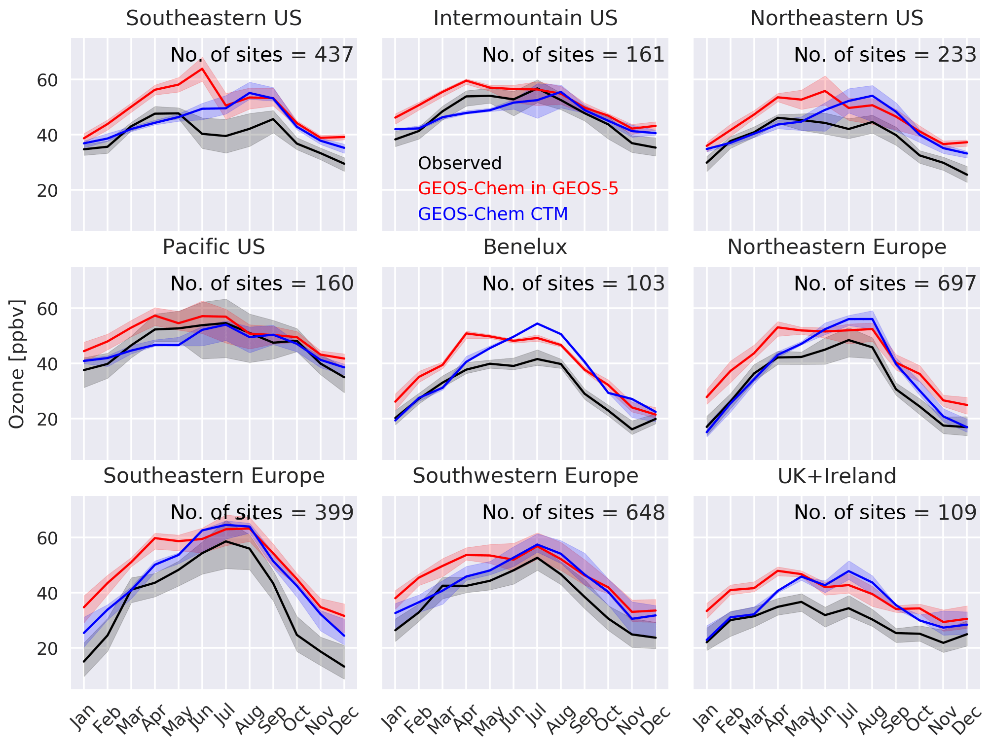
Figure 7Monthly median afternoon (12:00–16:00 LT) ozone concentrations (ppbv) for 2013–2014 at surface sites in the US and Europe, with interquartile range shaded. Surface monitoring sites are grouped according to Fig. A2. Also shown are the GEOS-5 Nature Run with GEOS-Chem chemistry (red) and the offline GEOS-Chem CTM (blue). Hourly model outputs are sampled for the locations and time of observations at the surface (lowest) level.
Observational datasets are described in the above references. Briefly, global ozonesonde observations are extracted from the WOUDC (World Ozone and Ultraviolet Radiation Data Centre; http://www.woudc.org, last access: 14 September 2018) and NOAA ESRL-GMD (Earth System Research Laboratory – Global Monitoring Division; ftp://ftp.cmdl.noaa.gov/ozwv/Ozonesonde/, last access: 14 September 2018). Ozonesonde stations are grouped into coherent regions for model evaluation (Tilmes et al., 2012). OMI middle tropospheric ozone data at 700–400 hPa are from the Smithsonian Astrophysical Observatory (SAO TROPOZ) retrieval (Huang et al., 2017; Liu et al., 2010) and are regridded to resolution to reduce retrieval noise. The NASA SEAC4RS dataset for southeast US described by Toon et al. (2016) is filtered following Travis et al. (2016) to remove open fire plumes (CH3CN > 200 pptv), stratospheric air (O3∕CO > 1.25 mol mol−1), and urban plumes (NO2 > 4 ppbv). Hourly surface observations for ozone are taken from the European Environment Agency database (complied by Grange, 2017) and the US Environmental Protection Agency Air Quality System (http://aqsdr1.epa.gov/aqsweb/aqstmp/airdata/download_files.html#Raw, last access: 14 September 2018). Only “background” sites are considered in the analysis: for the US, this includes sites defined by the EPA as “suburban” and “rural”; for Europe, this includes sites categorized as “urban background”, “background”, and “rural” (see Fig. A2).
4.2 Global burdens
Standard global metrics for evaluation of tropospheric chemistry models include the global burdens of tropospheric ozone, CO, and OH (Table 1). The global annual average ozone burden in G5NR-chem amounts to 348 Tg, consistent with the GEOS-Chem CTM and the Tropospheric Ozone Assessment Report (Hu et al., 2017; Young et al., 2018). The global burden of tropospheric CO of 294 Tg is consistent with the GEOS-Chem CTM and on the low end of the observationally based estimate of Gaubert et al. (2016). The global mean OH concentration is lower than in the GEOS-Chem CTM and more consistent with observational constraints (Prather et al., 2012; Prinn et al., 2005). The differences appear to be mainly driven by differences in the meteorological data.
4.3 Free tropospheric evaluation: OMI, ozonesonde, SEAC4RS
Figure 3 compares the GEOS-5 Nature Run with GEOS-Chem chemistry to OMI midtropospheric ozone. GEOS-Chem CTM results from Hu et al. (2017) are also shown. OMI data have been reprocessed with a single fixed a priori profile (so that variability is solely due to observations), corrected for their global mean bias relative to ozonesondes, and filtered for high latitudes because of large biases (Hu et al., 2017). Model outputs are sampled along the OMI tracks and smoothed with the OMI averaging kernels. G5NR-chem captures well-known major features of the ozone distribution, such as ozone enhancements at northern midlatitudes during MAM and JJA, and downwind of South America and Africa during SON. It shows no significant global bias relative to OMI and relative to the offline GEOS-Chem CTM. The global mean seasonal biases are less than 2.7±3.2 ppbv. Spatial correlations for the four seasons on the grid scale are high and show no significant latitudinal bias (; Fig. 4).
Figure 5 further evaluates the simulated vertical distribution of ozone in comparison to ozonesonde data. There are differences between G5NR-chem and the GEOS-Chem CTM that could be due to a number of factors including differences in tropopause altitude and the distribution of lightning. For example, although the annual total lightning NOx emission in G5NR-chem is scaled to that in GEOS-Chem CTM, the lightning location is not constrained by satellite lightning flash data as the CTM is. Annual mean ozone biases in G5NR-chem are generally less than 6 ppbv in the lower troposphere. There are some larger biases in the upper troposphere including differences with the GEOS-Chem CTM that could be due to the spatial distribution of lightning. Overall, G5NR-chem tends to improve the simulation of ozone vertical profiles compared to the GEOS-Chem CTM, most dramatically at high southern latitudes.
Figure 6 compares the model to mean vertical profiles of ozone and precursors measured over the southeast US during the SEAC4RS aircraft campaign. Here, the GEOS-Chem CTM results are from a nested simulation by Travis et al. (2016). The lower ozone in the northern midlatitude upper troposphere in G5NR-chem appears to be due to a weaker lightning NOx source. G5NR-chem overestimates ozone in the lower troposphere by 10 ppbv, while such bias is reduced in the GEOS-Chem CTM, even through both show almost identical NOx levels. The lower HCHO over the southeast US is due to weaker isoprene emission because of lower temperatures. Both models underestimate CO in the free troposphere but the bias is more apparent in the CTM, likely due to differences in fire emissions, global OH fields, or transport error in offline simulations (Yu et al., 2018).
4.4 Evaluation with surface observations over the US and Europe
Figure 7 shows monthly median surface ozone concentrations grouped by regions in the US and Europe. Here, hourly data between 12:00 and 16:00 LT are used to remove the known issue that models typically underestimate the ozone nighttime depletion at surface sites (Millet et al., 2015). G5NR-chem systematically overestimates surface ozone in almost all months by about 10 ppbv in all regions, while the GEOS-Chem CTM has no or small bias in winter and spring, but shows similar overestimates as in G5NR-chem during summer and fall. In general, the GEOS-5 Nature Run with GEOS-Chem chemistry better captures the observed seasonality. Expanding the analysis to all hourly data does not affect the systematic bias in G5NR-chem significantly but tends to increases the summer–fall bias in the CTM (Fig. A5). Part of the systematic bias is due to the subgrid vertical gradient between the lowest model level and the measurement altitude (Travis et al., 2017). Recent model developments such as improved halogen chemistry, aromatic chemistry, and ozone dry deposition are expected to reduce the surface high bias (Schmidt et al., 2016; Sherwen et al., 2016a, b, 2017; Silva and Heald, 2018; Yan et al., 2018). These updates are being incorporated into the GEOS-Chem version currently under development and will be passed on to the GEOS-5 simulation as they become available.
We presented a 1-year global simulation of tropospheric chemistry within the NASA GEOS ESM version 5 (GEOS-5) at cubed-sphere c720 () resolution. This demonstrated the success of implementing the GEOS-Chem chemical module within an ESM for online simulations with detailed chemistry. The GEOS-Chem chemical module online within GEOS and offline as the GEOS-Chem CTM uses exactly the same code. In this way, the continual stream of chemical updates from the large GEOS-Chem CTM community can be seamlessly incorporated as updates to the online model, which always remains state of the science and referenceable to the latest version of the GEOS-Chem. This 1-year simulation addressed an immediate need to generate the Nature Run for OSSEs in support of the geostationary satellite constellation for tropospheric chemistry. More broadly, implementation of the GEOS-Chem capability opens up a new capability for GEOS to address aerosol–chemistry–climate interactions, to assimilate satellite data of atmospheric composition, and to develop global air quality forecasts.
The 1-year GEOS-5 simulation at c720 resolution required 31 days of wall time on 4705 cores. Overall, 45 % of the wall time was spent on model dynamics and physics, 31 % on input/output, and 24 % on chemistry. Chemistry has near-perfect scalability in massively parallel architectures because it operates on individual grid columns; thus, it is no longer a computing bottleneck in ESM simulations. Transporting the large number of species involved in atmospheric chemistry simulations may be a greater challenge.
We evaluated the GEOS-5 Nature Run with GEOS-Chem chemistry for consistency with the offline GEOS-Chem CTM at coarser resolution ( global and nested over North America) as well as an ensemble of global observations for tropospheric ozone and aircraft observations of ozone precursors over the southeast US. The model shows no significant global bias relative to OMI midtropospheric ozone data and the offline GEOS-Chem CTM. Evaluations with ozonesondes show reduced model biases for high-latitude ozone. The GEOS-5 Nature Run with GEOS-Chem chemistry systematically overestimates surface ozone concentrations by 10 ppbv all year round in the US and Europe but is able to capture the observed seasonality, while the offline GEOS-Chem CTM reproduces observed surface ozone levels in winter and spring but has similar biases in summer and fall in all regions. Resolving this surface bias is presently a focus of attention in the GEOS-Chem CTM community and future model updates to address that bias can then be readily implemented into GEOS-5.
GEOS-Chem CTM is available at http://geos-chem.org/ (last access: 14 September 2018). GEOS-5 is available at https://geos5.org/wiki/index.php?title=GEOS-5_public_AGCM_Documentation_and_Access (last access: 14 September 2018).
All model outputs are available for download at https://portal.nccs.nasa.gov/datashare/G5NR-Chem/Heracles/12.5km/DATA (last access: 14 September 2018) or can be accessed through the OpenDAP framework at the portal https://opendap.nccs.nasa.gov/dods/OSSE/G5NR-Chem/Heracles/12.5km (last access: 14 September 2018).
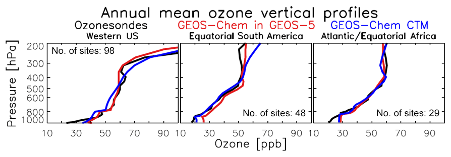
Figure A1Same as Fig. 5 but for western US, equatorial South America, and Atlantic/equatorial Africa.
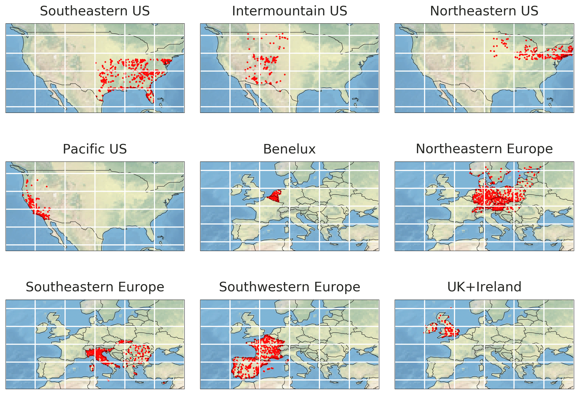
Figure A2Surface monitoring sites in the US and Europe grouped by subregions as analyzed in the text. Background image © Natural Earth (public domain license).
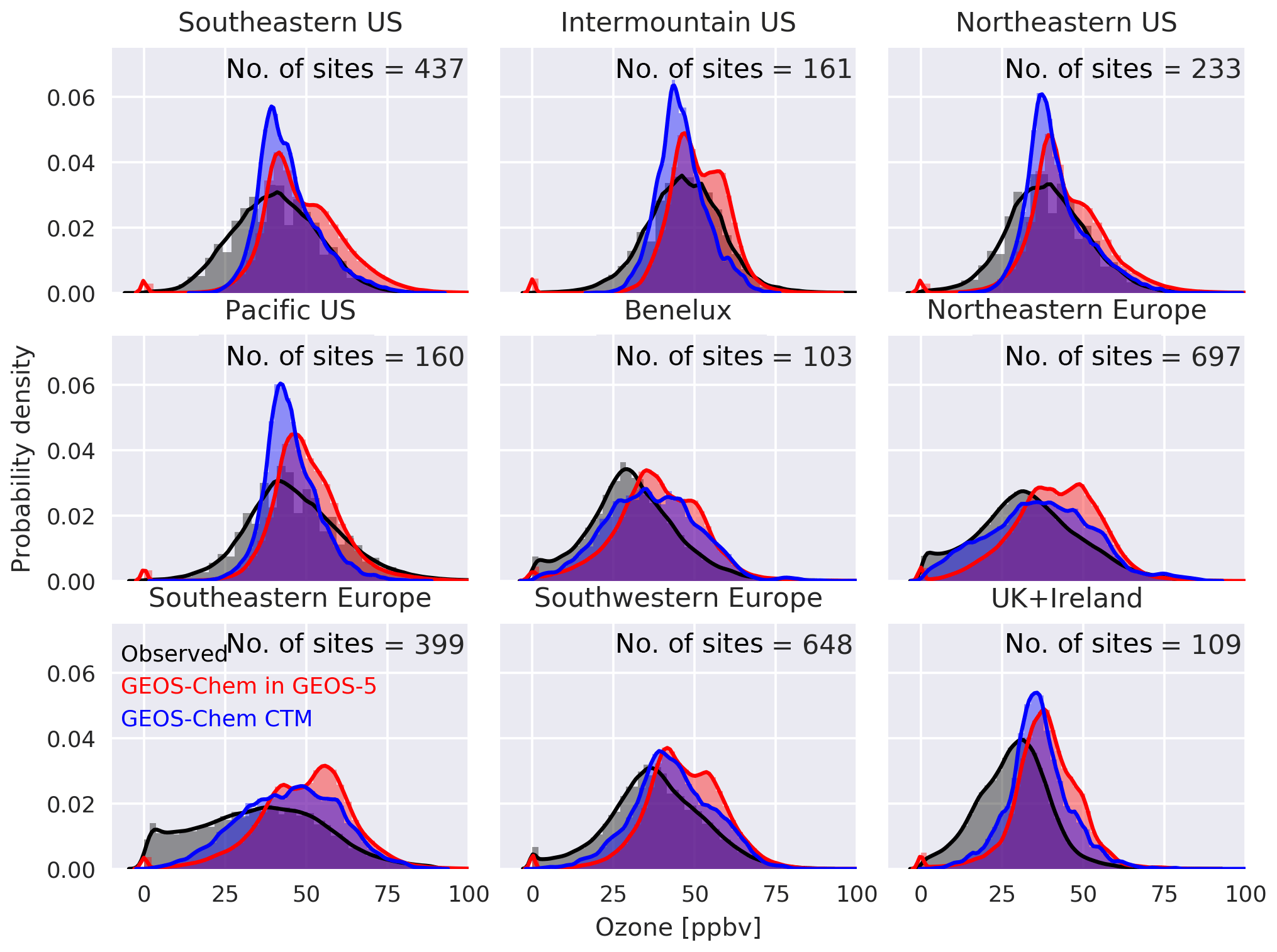
Figure A3Probability distribution of afternoon (12:00–16:00 LT) ozone concentrations (ppbv) for 2013–2014 at surface sites in the US and Europe.
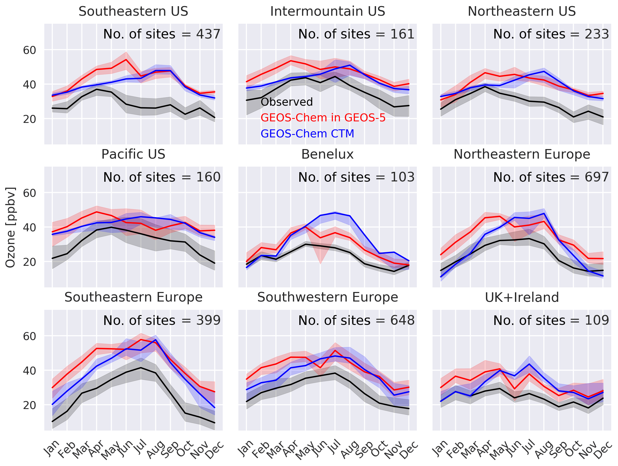
Figure A4Monthly median ozone concentrations (ppbv; all 24 h data) for 2013–2014 at surface sites in the US and Europe, with interquartile range shaded. Surface monitoring sites are grouped according to Fig. A2. Also shown are the GEOS-5 Nature Run with GEOS-Chem chemistry (red) and the offline GEOS-Chem CTM (blue). Hourly model outputs are sampled for the locations and time of observations at the surface (lowest) level.
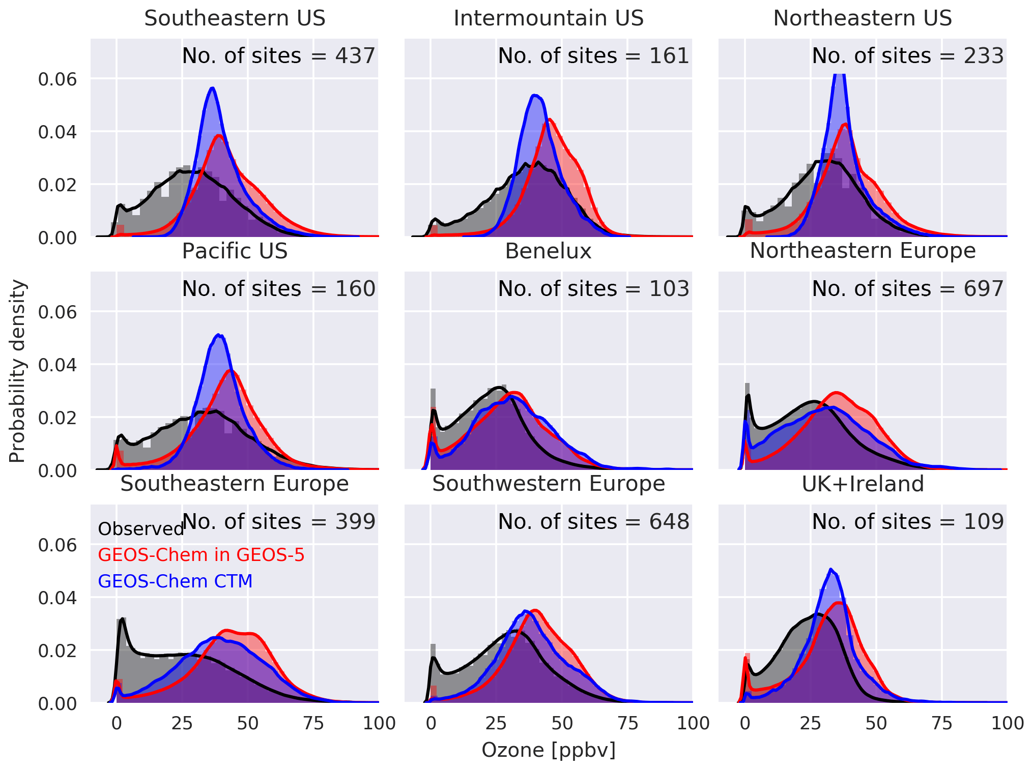
Figure A5Probability distribution of ozone concentrations (ppbv; all 24 h data) for 2013–2014 at surface sites in the US and Europe.
Table A1Computing resources for the GEOS-5 Nature Run with GEOS-Chem chemistrya.
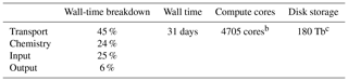
a The simulation is from 1 July 2013 to 1 July 2014 in GEOS ESM with GEOS-Chem as a chemical module at 12.5×12.5 km2. The computation was carried out at NASA Discover supercomputing cluster. b The simulation uses 337 14-core 2.6 GHz Intel Xeon Haswell compute nodes with 128 GB of memory per node and an Infiniband FDR interconnect using the Intel compiler suite (v. 15.0.0.090) and MPT v. 2.11. c 158 species are simulated and transported by the GEOS ESM; among them, 29 species are saved out as hourly outputs. Data are available at https://portal.nccs.nasa.gov/datashare/G5NR-Chem/Heracles/12.5km/DATA/ (last access: 14 September 2018).
Table A2Emissions in the GEOS-5 Nature Run with GEOS-Chem chemistry.
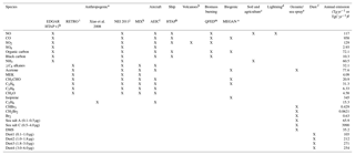
a Excluding aircraft and ships, which are listed separately. b http://aerocom.met.no/download/emissions/AEROCOM_HC/volc/ (last access: 14 September 2018). c Hudman et al. (2012). d Murray et al. (2012). e Jaeglé et al. (2011) and Fischer et al. (2012). f Zender et al. (2003). g TgC yr−1 for ≥C4 alkanes, acetone, methyl ethyl ketone (MEK), CH3CHO, C3H6, C3H8, isoprene, and C2H6. Tg yr−1 for the rest of the species. h http://edgar.jrc.ec.europa.eu/htap_v2/index.php?SECURE=123 (last access: 14 September 2018). i RETRO monthly global inventory for the year 2000 (Schultz et al., 2007) implemented as described by Hu et al. (2015a). j US EPA National Emission Inventory 2008 (http://www.epa.gov/ttn/chief/net/2008report.pdf; last access: 14 September 2018) and scaled to 2013 (https://www3.epa.gov/airtrends/; last access: 14 September 2018). k Asian anthropogenic emissions (Li et al., 2014). l Stettler et al. (2011). m Quick Fire Emissions Dataset (QFED) version 2.4-r6 (Darmenov and Da Silva, 2015). n MEGANv2.1 (Guenther et al., 2012) implemented in GEOS-Chem as described by Hu et al. (2015b).
SP and DJJ provided project oversight and top-level design. CAK, MSL, BA, ADS, JEN, MAT, and ALT performed code development and tests. KRT, SKG, and MJE provided additional data for model evaluation. LH, CAK, and TS performed evaluation analysis. LH, CAK, and DJJ wrote the manuscript. All authors contributed to manuscript editing and revisions.
The authors declare that they have no conflict of interest.
This work was supported by the NASA Modeling, Analysis, and Prediction
Program (MAP). Resources supporting the GEOS-5 simulations were provided by
the NASA Center for Climate Simulation at Goddard Space Flight Center. Lu Hu
acknowledges high-performance computing support from NCAR's
Computational and Information Systems Laboratory, sponsored by the National Science Foundation. Mat
J. Evans and Tomás Sherwen acknowledge funding for the computational
resource to perform the GEOS-Chem CTM model run from UK Natural Environment
Research Council (NERC, BACCHUS project NE/L01291X/1). We also acknowledge
all contributors to the ozonesonde data retrieved from the World Ozone and
Ultraviolet Radiation Data Centre (WOUDC) website
(http://www.woudc.org, last access: 14 September 2018).
Edited by: Fiona O'Connor
Reviewed by: two anonymous referees
Amos, H. M., Jacob, D. J., Holmes, C. D., Fisher, J. A., Wang, Q., Yantosca, R. M., Corbitt, E. S., Galarneau, E., Rutter, A. P., Gustin, M. S., Steffen, A., Schauer, J. J., Graydon, J. A., Louis, V. L. S., Talbot, R. W., Edgerton, E. S., Zhang, Y., and Sunderland, E. M.: Gas-particle partitioning of atmospheric Hg(II) and its effect on global mercury deposition, Atmos. Chem. Phys., 12, 591–603, https://doi.org/10.5194/acp-12-591-2012, 2012. a, b
Barré, J., Edwards, D., Worden, H., Arellano, A., Gaubert, B., Silva, A. D., Lahoz, W., and Anderson, J.: On the feasibility of monitoring carbon monoxide in the lower troposphere from a constellation of northern hemisphere geostationary satellites: Global scale assimilation experiments (Part II), Atmos. Environ., 140, 188–201, https://doi.org/10.1016/j.atmosenv.2016.06.001, 2016. a
Bian, H. and Prather, M. J.: Fast-J2: Accurate Simulation of Stratospheric Photolysis in Global Chemical Models, J. Atmos. Chem., 41, 281–296, https://doi.org/10.1023/A:1014980619462, 2002. a
Claeyman, M., Attié, J.-L., Peuch, V.-H., El Amraoui, L., Lahoz, W. A., Josse, B., Joly, M., Barré, J., Ricaud, P., Massart, S., Piacentini, A., von Clarmann, T., Höpfner, M., Orphal, J., Flaud, J.-M., and Edwards, D. P.: A thermal infrared instrument onboard a geostationary platform for CO and O3 measurements in the lowermost troposphere: Observing System Simulation Experiments (OSSE), Atmos. Meas. Tech., 4, 1637–1661, https://doi.org/10.5194/amt-4-1637-2011, 2011. a
Cohen, A. J., Brauer, M., Burnett, R., Anderson, H. R., Frostad, J., Estep, K., Balakrishnan, K., Brunekreef, B., Dandona, L., Dandona, R., Feigin, V., Freedman, G., Hubbell, B., Jobling, A., Kan, H., Knibbs, L., Liu, Y., Martin, R., Morawska, L., Pope, C. A., Shin, H., Straif, K., Shaddick, G., Thomas, M., van Dingenen, R., van Donkelaar, A., Vos, T., Murray, C. J. L., and Forouzanfar, M. H.: Estimates and 25-year trends of the global burden of disease attributable to ambient air pollution: an analysis of data from the Global Burden of Diseases Study 2015, The Lancet, 389, 1907–1918, https://doi.org/10.1016/S0140-6736(17)30505-6, 2017. a
Computational and Information Systems Laboratory: Cheyenne: HPE/SGI ICE XA System (University Community Computing). Boulder, CO: National Center for Atmospheric Research, https://doi.org/10.5065/D6RX99HX, 2017. a
Darmenov, A. S. and Da Silva, A. M.: The Quick Fire Emissions Dataset (QFED): Documentation of versions 2.1, 2.2 and 2.4., NASA Technical Report Series on Global Modeling and Data Assimilation 38, nASA/TM-2015-104606, 2015. a, b
Eastham, S. D., Weisenstein, D. K., and Barrett, S. R.: Development and evaluation of the unified tropospheric-stratospheric chemistry extension (UCX) for the global chemistry-transport model GEOS-Chem, Atmos. Environ., 89, 52–63, https://doi.org/10.1016/j.atmosenv.2014.02.001, 2014. a
Eastham, S. D., Long, M. S., Keller, C. A., Lundgren, E., Yantosca, R. M., Zhuang, J., Li, C., Lee, C. J., Yannetti, M., Auer, B. M., Clune, T. L., Kouatchou, J., Putman, W. M., Thompson, M. A., Trayanov, A. L., Molod, A. M., Martin, R. V., and Jacob, D. J.: GEOS-Chem High Performance (GCHP v11-02c): a next-generation implementation of the GEOS-Chem chemical transport model for massively parallel applications, Geosci. Model Dev., 11, 2941–2953, https://doi.org/10.5194/gmd-11-2941-2018, 2018. a
Fairlie, T. D., Jacob, D. J., and Park, R. J.: The impact of transpacific transport of mineral dust in the United States, Atmos. Environ., 41, 1251–1266, https://doi.org/10.1016/j.atmosenv.2006.09.048, 2007. a
Fischer, E. V., Jacob, D. J., Millet, D. B., Yantosca, R. M., and Mao, J.: The role of the ocean in the global atmospheric budget of acetone, Geophys. Res. Lett., 39, L01807, https://doi.org/10.1029/2011GL050086, 2012. a
Fishman, J., Iraci, L. T., Al-Saadi, J., Chance, K., Chavez, F., Chin, M., Coble, P., Davis, C., DiGiacomo, P. M., Edwards, D., Eldering, A., Goes, J., Herman, J., Hu, C., Jacob, D. J., Jordan, C., Kawa, S. R., Key, R., Liu, X., Lohrenz, S., Mannino, A., Natraj, V., Neil, D., Neu, J., Newchurch, M., Pickering, K., Salisbury, J., Sosik, H., Subramaniam, A., Tzortziou, M., Wang, J., and Wang, M.: The United States' Next Generation of Atmospheric Composition and Coastal Ecosystem Measurements: NASA's Geostationary Coastal and Air Pollution Events (GEO-CAPE) Mission, B. Am. Meteorol. Soc., 93, 1547–1566, https://doi.org/10.1175/BAMS-D-11-00201.1, 2012. a
Gaubert, B., Arellano, A. F., Barré, J., Worden, H. M., Emmons, L. K., Tilmes, S., Buchholz, R. R., Vitt, F., Raeder, K., Collins, N., Anderson, J. L., Wiedinmyer, C., Martinez Alonso, S., Edwards, D. P., Andreae, M. O., Hannigan, J. W., Petri, C., Strong, K., and Jones, N.: Toward a chemical reanalysis in a coupled chemistry-climate model: An evaluation of MOPITT CO assimilation and its impact on tropospheric composition, J. Geophys. Res.-Atmos., 121, 7310–7343, https://doi.org/10.1002/2016JD024863, 2016. a, b
Gelaro, R., McCarty, W., Suárez, M. J., Todling, R., Molod, A., Takacs, L., Randles, C. A., Darmenov, A., Bosilovich, M. G., Reichle, R., Wargan, K., Coy, L., Cullather, R., Draper, C., Akella, S., Buchard, V., Conaty, A., da Silva, A. M., Gu, W., Kim, G.-K., Koster, R., Lucchesi, R., Merkova, D., Nielsen, J. E., Partyka, G., Pawson, S., Putman, W., Rienecker, M., Schubert, S. D., Sienkiewicz, M., and Zhao, B.: The Modern-Era Retrospective Analysis for Research and Applications, Version 2 (MERRA-2), J. Climate, 30, 5419–5454, https://doi.org/10.1175/JCLI-D-16-0758.1, 2017. a
Grange, S. K.: Technical note: smonitor Europe (Version 1.0.1), Tech. rep., Wolfson Atmospheric Chemistry Laboratories, University of York, https://doi.org/10.13140/RG.2.2.20555.49448, 2017. a, b
Guenther, A. B., Jiang, X., Heald, C. L., Sakulyanontvittaya, T., Duhl, T., Emmons, L. K., and Wang, X.: The Model of Emissions of Gases and Aerosols from Nature version 2.1 (MEGAN2.1): an extended and updated framework for modeling biogenic emissions, Geosci. Model Dev., 5, 1471–1492, https://doi.org/10.5194/gmd-5-1471-2012, 2012. a, b
Hill, C., DeLuca, C., Balaji, V., Suarez, M., and Silva, A. D.: The Architecture of the Earth System Modeling Framework, Comput. Sci. Eng., 6, 18–28, https://doi.org/10.1109/MCISE.2004.1255817, 2004. a
Hu, L., Millet, D. B., Baasandorj, M., Griffis, T. J., Travis, K. R., Tessum, C. W., Marshall, J. D., Reinhart, W. F., Mikoviny, T., Müller, M., Wisthaler, A., Graus, M., Warneke, C., and Gouw, J.: Emissions of C6–C8 aromatic compounds in the United States: Constraints from tall tower and aircraft measurements, J. Geophys. Res.-Atmos., 120, 826–842, https://doi.org/10.1002/2014JD022627, 2015a. a
Hu, L., Millet, D. B., Baasandorj, M., Griffis, T. J., Turner, P., Helmig, D., Curtis, A. J., and Hueber, J.: Isoprene emissions and impacts over an ecological transition region in the U.S. Upper Midwest inferred from tall tower measurements, J. Geophys. Res., 120, 3553–3571, https://doi.org/10.1002/2014JD022732, 2015b. a, b
Hu, L., Jacob, D. J., Liu, X., Zhang, Y., Zhang, L., Kim, P. S., Sulprizio, M. P., and Yantosca, R. M.: Global budget of tropospheric ozone: Evaluating recent model advances with satellite (OMI), aircraft (IAGOS), and ozonesonde observations, Atmos. Environ., 167, 323–334, https://doi.org/10.1016/j.atmosenv.2017.08.036, 2017. a, b, c, d, e, f, g, h, i, j, k, l
Huang, G., Liu, X., Chance, K., Yang, K., Bhartia, P. K., Cai, Z., Allaart, M., Ancellet, G., Calpini, B., Coetzee, G. J. R., Cuevas-Agulló, E., Cupeiro, M., De Backer, H., Dubey, M. K., Fuelberg, H. E., Fujiwara, M., Godin-Beekmann, S., Hall, T. J., Johnson, B., Joseph, E., Kivi, R., Kois, B., Komala, N., König-Langlo, G., Laneve, G., Leblanc, T., Marchand, M., Minschwaner, K. R., Morris, G., Newchurch, M. J., Ogino, S.-Y., Ohkawara, N., Piters, A. J. M., Posny, F., Querel, R., Scheele, R., Schmidlin, F. J., Schnell, R. C., Schrems, O., Selkirk, H., Shiotani, M., Skrivánková, P., Stübi, R., Taha, G., Tarasick, D. W., Thompson, A. M., Thouret, V., Tully, M. B., Van Malderen, R., Vömel, H., von der Gathen, P., Witte, J. C., and Yela, M.: Validation of 10-year SAO OMI Ozone Profile (PROFOZ) product using ozonesonde observations, Atmos. Meas. Tech., 10, 2455–2475, https://doi.org/10.5194/amt-10-2455-2017, 2017. a
Hudman, R. C., Moore, N. E., Mebust, A. K., Martin, R. V., Russell, A. R., Valin, L. C., and Cohen, R. C.: Steps towards a mechanistic model of global soil nitric oxide emissions: implementation and space based-constraints, Atmos. Chem. Phys., 12, 7779–7795, https://doi.org/10.5194/acp-12-7779-2012, 2012. a
Jaeglé, L., Quinn, P. K., Bates, T. S., Alexander, B., and Lin, J.-T.: Global distribution of sea salt aerosols: new constraints from in situ and remote sensing observations, Atmos. Chem. Phys., 11, 3137–3157, https://doi.org/10.5194/acp-11-3137-2011, 2011. a, b, c
Keller, C. A., Long, M. S., Yantosca, R. M., Da Silva, A. M., Pawson, S., and Jacob, D. J.: HEMCO v1.0: a versatile, ESMF-compliant component for calculating emissions in atmospheric models, Geosci. Model Dev., 7, 1409–1417, https://doi.org/10.5194/gmd-7-1409-2014, 2014. a, b, c
Kim, P. S., Jacob, D. J., Fisher, J. A., Travis, K., Yu, K., Zhu, L., Yantosca, R. M., Sulprizio, M. P., Jimenez, J. L., Campuzano-Jost, P., Froyd, K. D., Liao, J., Hair, J. W., Fenn, M. A., Butler, C. F., Wagner, N. L., Gordon, T. D., Welti, A., Wennberg, P. O., Crounse, J. D., St. Clair, J. M., Teng, A. P., Millet, D. B., Schwarz, J. P., Markovic, M. Z., and Perring, A. E.: Sources, seasonality, and trends of southeast US aerosol: an integrated analysis of surface, aircraft, and satellite observations with the GEOS-Chem chemical transport model, Atmos. Chem. Phys., 15, 10411–10433, https://doi.org/10.5194/acp-15-10411-2015, 2015. a
Li, M., Zhang, Q., Streets, D. G., He, K. B., Cheng, Y. F., Emmons, L. K., Huo, H., Kang, S. C., Lu, Z., Shao, M., Su, H., Yu, X., and Zhang, Y.: Mapping Asian anthropogenic emissions of non-methane volatile organic compounds to multiple chemical mechanisms, Atmos. Chem. Phys., 14, 5617–5638, https://doi.org/10.5194/acp-14-5617-2014, 2014. a
Liu, H., Jacob, D. J., Bey, I., and Yantosca, R. M.: Constraints from 210Pb and 7Be on wet deposition and transport in a global three-dimensional chemical tracer model driven by assimilated meteorological fields, J. Geophys. Res.-Atmos., 106, 12109–12128, https://doi.org/10.1029/2000JD900839, 2001. a, b
Liu, X., Bhartia, P. K., Chance, K., Spurr, R. J. D., and Kurosu, T. P.: Ozone profile retrievals from the Ozone Monitoring Instrument, Atmos. Chemi. Phys., 10, 2521–2537, https://doi.org/10.5194/acp-10-2521-2010, 2010. a
Lock, A. P., Brown, A. R., Bush, M. R., Martin, G. M., and Smith, R. N. B.: A New Boundary Layer Mixing Scheme. Part I: Scheme Description and Single-Column Model Tests, Mon. Weather Rev., 128, 3187–3199, https://doi.org/10.1175/1520-0493(2000)128<3187:ANBLMS>2.0.CO;2, 2000. a
Long, M. S., Yantosca, R., Nielsen, J. E., Keller, C. A., da Silva, A., Sulprizio, M. P., Pawson, S., and Jacob, D. J.: Development of a grid-independent GEOS-Chem chemical transport model (v9-02) as an atmospheric chemistry module for Earth system models, Geosci. Model Dev., 8, 595–602, https://doi.org/10.5194/gmd-8-595-2015, 2015. a, b, c, d, e
Louis, J.-F., Tiedtke, M., and Geleyn, J.-F.: A short history of the PBL parameterization at ECMWF, in: Workshop on Planetary Boundary Layer parameterization, 25–27 November 1981, 59–79, ECMWF, ECMWF, Shinfield Park, Reading, 1982. a
Mao, J., Jacob, D. J., Evans, M. J., Olson, J. R., Ren, X., Brune, W. H., Clair, J. M. S., Crounse, J. D., Spencer, K. M., Beaver, M. R., Wennberg, P. O., Cubison, M. J., Jimenez, J. L., Fried, A., Weibring, P., Walega, J. G., Hall, S. R., Weinheimer, A. J., Cohen, R. C., Chen, G., Crawford, J. H., McNaughton, C., Clarke, A. D., Jaeglé, L., Fisher, J. A., Yantosca, R. M., Le Sager, P., and Carouge, C.: Chemistry of hydrogen oxide radicals (HOx) in the Arctic troposphere in spring, Atmos. Chem. Phys., 10, 5823–5838, https://doi.org/10.5194/acp-10-5823-2010, 2010. a
Mao, J., Paulot, F., Jacob, D. J., Cohen, R. C., Crounse, J. D., Wennberg, P. O., Keller, C. A., Hudman, R. C., Barkley, M. P., and Horowitz, L. W.: Ozone and organic nitrates over the eastern United States: Sensitivity to isoprene chemistry, J. Geophysi. Res.-Atmos., 118, 11256–11268, https://doi.org/10.1002/jgrd.50817, 2013. a
McLinden, C. A., Olsen, S. C., Hannegan, B., Wild, O., Prather, M. J., and Sundet, J.: Stratospheric ozone in 3-D models: A simple chemistry and the cross-tropopause flux, J. Geophys. Res.-Atmos., 105, 14653–14665, https://doi.org/10.1029/2000JD900124, 2000. a
Millet, D. B., Baasandorj, M., Farmer, D. K., Thornton, J. A., Baumann, K., Brophy, P., Chaliyakunnel, S., de Gouw, J. A., Graus, M., Hu, L., Koss, A., Lee, B. H., Lopez-Hilfiker, F. D., Neuman, J. A., Paulot, F., Peischl, J., Pollack, I. B., Ryerson, T. B., Warneke, C., Williams, B. J., and Xu, J.: A large and ubiquitous source of atmospheric formic acid, Atmos. Chem. Phys., 15, 6283–6304, https://doi.org/10.5194/acp-15-6283-2015, 2015. a
Molod, A., Takacs, L., Suarez, M., and Bacmeister, J.: Development of the GEOS-5 atmospheric general circulation model: evolution from MERRA to MERRA2, Geosci. Model Dev., 8, 1339–1356, https://doi.org/10.5194/gmd-8-1339-2015, 2015. a, b
Moorthi, S. and Suarez, M. J.: Relaxed Arakawa-Schubert. A Parameterization of Moist Convection for General Circulation Models, Mon. Weather Rev., 120, 978–1002, 1992. a
Murray, L. T., Jacob, D. J., Logan, J. A., Hudman, R. C., and Koshak, W. J.: Optimized regional and interannual variability of lightning in a global chemical transport model constrained by LIS/OTD satellite data, J. Geophys. Res.-Atmos., 117, d20307, https://doi.org/10.1029/2012JD017934, 2012. a, b, c
Naik, V., Voulgarakis, A., Fiore, A. M., Horowitz, L. W., Lamarque, J.-F., Lin, M., Prather, M. J., Young, P. J., Bergmann, D., Cameron-Smith, P. J., Cionni, I., Collins, W. J., Dalsøren, S. B., Doherty, R., Eyring, V., Faluvegi, G., Folberth, G. A., Josse, B., Lee, Y. H., MacKenzie, I. A., Nagashima, T., van Noije, T. P. C., Plummer, D. A., Righi, M., Rumbold, S. T., Skeie, R., Shindell, D. T., Stevenson, D. S., Strode, S., Sudo, K., Szopa, S., and Zeng, G.: Preindustrial to present-day changes in tropospheric hydroxyl radical and methane lifetime from the Atmospheric Chemistry and Climate Model Intercomparison Project (ACCMIP), Atmos. Chem. Phys., 13, 5277–5298, https://doi.org/10.5194/acp-13-5277-2013, 2013. a
National Academies of Sciences, Engineering, and Medicine: The Future of Atmospheric Chemistry Research: Remembering Yesterday, Understanding Today, Anticipating Tomorrow, The National Academies Press, Washington DC, USA, https://doi.org/10.17226/23573, 2016. a
National Research Council: A National Strategy for Advancing Climate Modeling, The National Academies Press, Washington DC, USA, https://doi.org/10.17226/13430, 2012. a
Orbe, C., Oman, L. D., Strahan, S. E., Waugh, D. W., Pawson, S., Takacs, L. L., and Molod, A. M.: Large-Scale Atmospheric Transport in GEOS Replay Simulations, J. Adv. Model. Earth Syst., 9, 2545–2560, 2017. a
Park, R. J., Jacob, D. J., Field, B. D., Yantosca, R. M., and Chin, M.: Natural and transboundary pollution influences on sulfate-nitrate-ammonium aerosols in the United States: Implications for policy, J. Geophys. Res.-Atmos., 109, D004473, https://doi.org/10.1029/2003JD004473, 2004. a
Parrella, J. P., Jacob, D. J., Liang, Q., Zhang, Y., Mickley, L. J., Miller, B., Evans, M. J., Yang, X., Pyle, J. A., Theys, N., and Van Roozendael, M.: Tropospheric bromine chemistry: implications for present and pre-industrial ozone and mercury, Atmos. Chem. Phys., 12, 6723–6740, https://doi.org/10.5194/acp-12-6723-2012, 2012. a
Prather, M. J., Holmes, C. D., and Hsu, J.: Reactive greenhouse gas scenarios: Systematic exploration of uncertainties and the role of atmospheric chemistry, Geophys. Res. Lett., 39, l09803, https://doi.org/10.1029/2012GL051440, 2012. a
Prinn, R. G., Huang, J., Weiss, R. F., Cunnold, D. M., Fraser, P. J., Simmonds, P. G., McCulloch, A., Harth, C., Reimann, S., Salameh, P., O'Doherty, S., Wang, R. H. J., Porter, L. W., Miller, B. R., and Krummel, P. B.: Evidence for variability of atmospheric hydroxyl radicals over the past quarter century, Geophys. Res. Lett., 32, L07809, https://doi.org/10.1029/2004GL022228, 2005. a
Sander, S. P., Golden, D., Kurylo, M., Moortgat, G., Wine, P., Ravishankara, A., Kolb, C., Molina, M., Finlayson-Pitts, M., and Huie, R.: Chemical kinetics and photochemical data for use in atmospheric studies, JPL Publications, 06-2, 684, 2011. a
Schmidt, J. A., Jacob, D. J., Horowitz, H. M., Hu, L., Sherwen, T., Evans, M. J., Liang, Q., Suleiman, R. M., Oram, D. E., Breton, M. L., Percival, C. J., Wang, S., Dix, B., and Volkamer, R.: Modeling the observed tropospheric BrO background: Importance of multiphase chemistry and implications for ozone, OH, and mercury, J. Geophys. Res.-Atmos., 121, 11819–11835, https://doi.org/10.1002/2015JD024229, 2016. a
Schultz, M., Backman, L., Balkanski, Y., Bjoerndalsaeter, S., Brand, R., Burrows, J., Dalsoeren, S., de Vasconcelos, M., Grodtmann, B., Hauglustaine, D., Heil, A., Hoelzemann, J., Isaksen, I., Kaurola, J., Knorr, W., Ladstaetter-Weissenmayer, A., Mota, B., Oom, D., Pacyna, J., and Wittrock, F.: REanalysis of the TROpospheric chemical composition over the past 40 years, Project ID: EVK2-CT-2002-00170, 2007. a
Sherwen, T., Evans, M. J., Carpenter, L. J., Andrews, S. J., Lidster, R. T., Dix, B., Koenig, T. K., Sinreich, R., Ortega, I., Volkamer, R., Saiz-Lopez, A., Prados-Roman, C., Mahajan, A. S., and Ordóñez, C.: Iodine's impact on tropospheric oxidants: a global model study in GEOS-Chem, Atmos. Chem. Phys., 16, 1161–1186, https://doi.org/10.5194/acp-16-1161-2016, 2016a. a
Sherwen, T., Schmidt, J. A., Evans, M. J., Carpenter, L. J., Großmann, K., Eastham, S. D., Jacob, D. J., Dix, B., Koenig, T. K., Sinreich, R., Ortega, I., Volkamer, R., Saiz-Lopez, A., Prados-Roman, C., Mahajan, A. S., and Ordóñez, C.: Global impacts of tropospheric halogens (Cl, Br, I) on oxidants and composition in GEOS-Chem, Atmos. Chem. Phys., 16, 12239–12271, https://doi.org/10.5194/acp-16-12239-2016, 2016b. a
Sherwen, T., Evans, M. J., Sommariva, R., Hollis, L. D. J., Ball, S. M., Monks, P. S., Reed, C., Carpenter, L. J., Lee, J. D., Forster, G., Bandy, B., Reeves, C. E., and Bloss, W. J.: Effects of halogens on European air-quality, Faraday Discuss., 200, 75–100, https://doi.org/10.1039/C7FD00026J, 2017. a
Silva, S. J. and Heald, C. L.: Investigating Dry Deposition of Ozone to Vegetation, J. Geophys. Res.-Atmos., 123, 559–573, https://doi.org/10.1002/2017JD027278, 2018. a
Stettler, M., Eastham, S., and Barrett, S.: Air quality and public health impacts of UK airports. Part I: Emissions, Atmos. Environ., 45, 5415–5424, https://doi.org/10.1016/j.atmosenv.2011.07.012, 2011. a
Tilmes, S., Lamarque, J.-F., Emmons, L. K., Conley, A., Schultz, M. G., Saunois, M., Thouret, V., Thompson, A. M., Oltmans, S. J., Johnson, B., and Tarasick, D.: Technical Note: Ozonesonde climatology between 1995 and 2011: description, evaluation and applications, Atmos. Chem. Phys., 12, 7475–7497, https://doi.org/10.5194/acp-12-7475-2012, 2012. a, b
Toon, O. B., Maring, H., Dibb, J., Ferrare, R., Jacob, D. J., Jensen, E. J., Luo, Z. J., Mace, G. G., Pan, L. L., Pfister, L., Rosenlof, K. H., Redemann, J., Reid, J. S., Singh, H. B., Thompson, A. M., Yokelson, R., Minnis, P., Chen, G., Jucks, K. W., and Pszenny, A.: Planning, implementation, and scientific goals of the Studies of Emissions and Atmospheric Composition, Clouds and Climate Coupling by Regional Surveys (SEAC4RS) field mission, J. Geophys. Res.-Atmos., 121, 4967–5009, https://doi.org/10.1002/2015JD024297, 2016. a, b
Travis, K. R., Jacob, D. J., Fisher, J. A., Kim, P. S., Marais, E. A., Zhu, L., Yu, K., Miller, C. C., Yantosca, R. M., Sulprizio, M. P., Thompson, A. M., Wennberg, P. O., Crounse, J. D., St. Clair, J. M., Cohen, R. C., Laughner, J. L., Dibb, J. E., Hall, S. R., Ullmann, K., Wolfe, G. M., Pollack, I. B., Peischl, J., Neuman, J. A., and Zhou, X.: Why do models overestimate surface ozone in the Southeast United States?, Atmos. Chem. Phys., 16, 13561–13577, https://doi.org/10.5194/acp-16-13561-2016, 2016. a, b, c, d, e
Travis, K. R., Jacob, D. J., Keller, C. A., Kuang, S., Lin, J., Newchurch, M. J., and Thompson, A. M.: Resolving ozone vertical gradients in air quality models, Atmos. Chem. Phys. Discuss., https://doi.org/10.5194/acp-2017-596, 2017. a
Trivitayanurak, W., Adams, P. J., Spracklen, D. V., and Carslaw, K. S.: Tropospheric aerosol microphysics simulation with assimilated meteorology: model description and intermodel comparison, Atmos. Chem. Phys., 8, 3149–3168, https://doi.org/10.5194/acp-8-3149-2008, 2008. a
Vinken, G. C. M., Boersma, K. F., Jacob, D. J., and Meijer, E. W.: Accounting for non-linear chemistry of ship plumes in the GEOS-Chem global chemistry transport model, Atmospheric Chemistry and Physics, 11, 11707–11722, https://doi.org/10.5194/acp-11-11707-2011, 2011. a
Wang, Q., Jacob, D. J., Spackman, J. R., Perring, A. E., Schwarz, J. P., Moteki, N., Marais, E. A., Ge, C., Wang, J., and Barrett, S. R. H.: Global budget and radiative forcing of black carbon aerosol: Constraints from pole-to-pole (HIPPO) observations across the Pacific, J. Geophys. Res.-Atmos., 119, 195–206, 2014. a
Wang, Y., Jacob, D. J., and Logan, J. A.: Global simulation of tropospheric O3−NOx-hydrocarbon chemistry: 3. Origin of tropospheric ozone and effects of nonmethane hydrocarbons, J. Geophys. Res., 103, 10757–10767, 1998. a
Wesely, M.: Parameterization of surface resistances to gaseous dry deposition in regional-scale numerical models, Atmos. Environ., 23, 1293–1304, 1989. a
Xiao, Y., Logan, J. A., Jacob, D. J., Hudman, R. C., Yantosca, R., and Blake, D. R.: Global budget of ethane and regional constraints on U.S. sources, J. Geophys. Res.-Atmos., 113, d21306, https://doi.org/10.1029/2007JD009415, 2008. a
Yan, Y., Lin, J., Chen, J., and Hu, L.: Improved simulation of tropospheric ozone by a global-multi-regional two-way coupling model system, Atmos. Chem. Phys., 16, 2381–2400, https://doi.org/10.5194/acp-16-2381-2016, 2016. a
Yan, Y., Cabrera-Perez, D., Lin, J., Pozzer, A., Hu, L., Millet, D. B., Porter, W. C., and Lelieveld, J.: Global tropospheric effects of aromatic chemistry with the SAPRC-11 mechanism implemented in GEOS-Chem, Geosci. Model Dev. Discuss., https://doi.org/10.5194/gmd-2018-196, in review, 2018. a
Young, P. J., Naik, V., Fiore, A. M., Gaudel, A., Guo, J., Lin, M. Y., Neu, J. L., Parrish, D. D., Rieder, H. E., Schnell, J. L., Tilmes, S., Wild, O., Zhang, L., Ziemke, J. R., Brandt, J., Delcloo, A., Doherty, R. M., Geels, C., Hegglin, M. I., Hu, L., Im, U., Kumar, R., Luhar, A., Murray, L., Plummer, D., Rodriguez, J., Saiz-Lopez, A., Schultz, M. G., Woodhouse, M. T., and Zeng, G.: Tropospheric Ozone Assessment Report: Assessment of global-scale model performance for global and regional ozone distributions, variability, and trends, Elem. Sci. Anth., 6, 10, https://doi.org/10.1525/elementa.265, 2018. a, b
Yu, F. and Luo, G.: Simulation of particle size distribution with a global aerosol model: contribution of nucleation to aerosol and CCN number concentrations, Atmos. Chem. Phys., 9, 7691–7710, https://doi.org/10.5194/acp-9-7691-2009, 2009. a
Yu, K., Keller, C. A., Jacob, D. J., Molod, A. M., Eastham, S. D., and Long, M. S.: Errors and improvements in the use of archived meteorological data for chemical transport modeling: an analysis using GEOS-Chem v11-01 driven by GEOS-5 meteorology, Geosci. Model Dev., 11, 305–319, https://doi.org/10.5194/gmd-11-305-2018, 2018. a, b, c, d
Yumimoto, K.: Impacts of geostationary satellite measurements on CO forecasting: An observing system simulation experiment with GEOS-Chem/LETKF data assimilation system, Atmos. Environ., 74, 123–133, https://doi.org/10.1016/j.atmosenv.2013.03.032, 2013. a
Zender, C. S., Bian, H., and Newman, D.: Mineral Dust Entrainment and Deposition (DEAD) model: Description and 1990s dust climatology, J. Geophys. Res.-Atmos., 108, 4416, https://doi.org/10.1029/2002JD002775, 2003. a, b
Zoogman, P., Jacob, D. J., Chance, K., Liu, X., Lin, M., Fiore, A., and Travis, K.: Monitoring high-ozone events in the US Intermountain West using TEMPO geostationary satellite observations, Atmos. Chem. Phys., 14, 6261–6271, https://doi.org/10.5194/acp-14-6261-2014, 2014. a
Zoogman, P., Liu, X., Suleiman, R., Pennington, W., Flittner, D., Al-Saadi, J., Hilton, B., Nicks, D., Newchurch, M., Carr, J., Janz, S., Andraschko, M., Arola, A., Baker, B., Canova, B., Miller, C. C., Cohen, R., Davis, J., Dussault, M., Edwards, D., Fishman, J., Ghulam, A., Abad, G. G., Grutter, M., Herman, J., Houck, J., Jacob, D., Joiner, J., Kerridge, B., Kim, J., Krotkov, N., Lamsal, L., Li, C., Lindfors, A., Martin, R., McElroy, C., McLinden, C., Natraj, V., Neil, D., Nowlan, C., O'Sullivan, E., Palmer, P., Pierce, R., Pippin, M., Saiz-Lopez, A., Spurr, R., Szykman, J., Torres, O., Veefkind, J., Veihelmann, B., Wang, H., Wang, J., and Chance, K.: Tropospheric emissions: Monitoring of pollution (TEMPO), J. Quant. Spectrosc. Rad. Transf., 186, 17–39, https://doi.org/10.1016/j.jqsrt.2016.05.008, 2017. a, b