the Creative Commons Attribution 4.0 License.
the Creative Commons Attribution 4.0 License.
 | 30 Nov 2018
Land surface model parameter optimisation using in situ flux data: comparison of gradient-based versus random search algorithms (a case study using ORCHIDEE v1.9.5.2)
Vladislav Bastrikov
Natasha MacBean
Cédric Bacour
Diego Santaren
Sylvain Kuppel
Philippe Peylin
Land surface models (LSMs), which form the land component of earth system models, rely on numerous processes for describing carbon, water and energy budgets, often associated with highly uncertain parameters. Data assimilation (DA) is a useful approach for optimising the most critical parameters in order to improve model accuracy and refine future climate predictions. In this study, we compare two different DA methods for optimising the parameters of seven plant functional types (PFTs) of the ORCHIDEE LSM using daily averaged eddy-covariance observations of net ecosystem exchange and latent heat flux at 78 sites across the globe. We perform a technical investigation of two classes of minimisation methods – local gradient-based (the L-BFGS-B algorithm, limited memory Broyden–Fletcher–Goldfarb–Shanno algorithm with bound constraints) and global random search (the genetic algorithm) – by evaluating their relative performance in terms of the model–data fit and the difference in retrieved parameter values. We examine the performance of each method for two cases: when optimising parameters at each site independently (“single-site” approach) and when simultaneously optimising the model at all sites for a given PFT using a common set of parameters (“multi-site” approach). We find that for the single site case the random search algorithm results in lower values of the cost function (i.e. lower model–data root mean square differences) than the gradient-based method; the difference between the two methods is smaller for the multi-site optimisation due to a smoothing of the cost function shape with a greater number of observations. The spread of the cost function, when performing the same tests with 16 random first-guess parameters, is much larger with the gradient-based method, due to the higher likelihood of being trapped in local minima. When using pseudo-observation tests, the genetic algorithm results in a closer approximation of the true posterior parameter value in the L-BFGS-B algorithm. We demonstrate the advantages and challenges of different DA techniques and provide some advice on using it for the LSM parameter optimisation.
- Article
(1405 KB) -
Supplement
(1435 KB) - BibTeX
- EndNote


In the context of climate change and the potentially large impact of global warming on terrestrial ecosystem functioning (with consequent feedbacks to climate), the development of reliable and robust process-driven land surface models (LSMs) to assess the future evolution of carbon, water and energy budgets is of key importance (Field and Raupach, 2004). These models also represent a major tool for understanding the underlying mechanics and interconnections between the terrestrial biosphere, the atmospheric composition and human environmental management practices (Cramer et al., 2001).
State-of-the-art LSMs include hundreds of processes describing energy and mass (water and carbon) transfers in the soil–plant–atmosphere continuum on a wide range of temporal and spatial scales. This inevitably leads to high model complexity due to interactions between biophysical and biogeochemical processes. The simulated carbon, water and energy fluxes and stocks thus remain highly uncertain (Anav et al., 2013; Friedlingstein et al., 2014; Sitch et al., 2015). These uncertainties typically arise from three main sources.
-
Errors in the input data: uncertainty in the meteorological forcing and/or the vegetation and soil spatial information used to drive the model;
-
Errors in the model structure: insufficient or erroneous description of biogeochemical and biophysical processes;
-
Errors in the model parameterisation: uncertain or incorrect values of the fixed values (parameters) used in the equations representing these processes.
The latter source of uncertainty is the focus of this study. Model parameter error can be due to insufficient availability or inadequacy of observations and experiments used to derive the model parameter values, or because the parameters themselves are “effective” and not directly observable in reality. In the former case, observations were usually limited to only a few experiments carried out at spatial and temporal scales that were not always relevant for larger-scale simulations. For instance, the observations correspond to experiments using only a few plant species, soil types or climatic regions, and thus typically did not encompass all the variability required of the vegetation classification used in LSMs based on the concept of plant functional types (PFTs). Parameter uncertainty can therefore lead to significant uncertainty in simulations of carbon, water and energy fluxes and stocks (Luo et al., 2016; Peylin et al., 2016; Raoult et al., 2016; Schürmann et al., 2016; Thum et al., 2017).
Fortunately, there are a growing number of observations as well as new types of measurements that should aid us in significantly reducing model parameter uncertainty. Among these observations, eddy-covariance measurements of net CO2 flux (net ecosystem exchange, NEE), water and energy fluxes at specific FLUXNET sites represent an unprecedented source of information on the diurnal to seasonal and interannual processes (Williams et al., 2009). More than 650 sites, operating on a long-term and continuous basis and covering major ecosystems of the world, are available (Baldocchi et al., 2001; http://fluxnet.fluxdata.org, last access: 26 November 2018). A large number of studies have used these flux measurements to optimise ecosystem model parameters, either using the data from one single site (SS) (Reichstein et al., 2003; Braswell et al., 2005; Moore et al., 2008; Ricciuto et al., 2011; Santaren et al., 2014; Kato et al., 2013; Bacour et al., 2015) or from multiple sites (MSs) simultaneously – usually at the level of PFTs (Groenendijk et al., 2011; Kuppel et al., 2014; Raoult et al., 2016). These studies have employed various data assimilation (DA) inversion approaches, but they all rely on a Bayesian framework that allows for the update of a priori information on the parameters (i.e. the parameter prior probability distribution functions, PDFs) using the new information contained in the observations, which results in the posterior PDFs. While some methods do not require any assumption as to the shape of the different PDFs (e.g. see Van Oijen et al., 2005, and Post et al., 2017, who use Markov Chain Monte Carlo, MCMC, methods), many inversion methods use Gaussian error assumptions (for both parameters and observations), which simplifies the characterisation of the posterior parameter PDFs and leads to the minimisation of a cost function (Dietze et al., 2013). Our study uses such a Gaussian hypothesis.
The optimisation requires the minimisation of a cost function that describes the difference between the model and the observations, taking into account their respective uncertainties. There is a wide variety of mathematical algorithms that can be used to explore the parameter space (in the case of DA for parameter estimation), and therefore for locating the minimum of a cost function. These methods can be broadly divided into two classes: (i) local gradient-based methods (i.e. gradient-descent or conjugate gradient algorithms for example) also referred to as variational, or 4-D-Var, methods; and (ii) global random search method (MCMC, genetic and particle filter algorithms are commonly used examples). There are various advantages and disadvantages for the different algorithms of each class, depending on the complexity of the model being optimised (mainly the degree of model non-linearity), the computational time of each model simulation and the number of parameters to be optimised. Random search methods (as used in Van Oijen et al., 2005; Richardson et al., 2010; and Post et al., 2017, for example) have been proven to be efficient at finding the correct parameter values with highly non-linear models but at the expense of potentially prohibitive computing cost. On the other hand, gradient-based methods (as used in Kuppel et al., 2014; Raoult et al., 2016; Pinnington et al., 2016; and Schürmann et al., 2016, for example) are more prone to getting stuck in local minima and, furthermore, they require the complex calculation of the gradient of the cost function with respect to all parameters. With idealised models, Chorin and Morzfeld (2013) have shown that the assimilation can be optimal with particle filters or variational methods, under the condition that the effective dimension of the problem (defined as the Frobenius norm of the steady-state posterior covariance) is finite. The choice of the minimisation method was shown to have little impact on the overall optimisation efficiency for relatively simple ecosystem models (Trudinger et al., 2007; Fox et al., 2009). Ziehn et al. (2012) showed similar performances between a MCMC and a variational method in terms of locating the minimum of the cost function for the BETHY ecosystem model (using atmospheric CO2 data as constraint), except for the difference in computational time (much longer using MCMC). However, with the more complex ORCHIDEE LSM, Santaren et al. (2014) showed that the genetic algorithm (GA) was superior to a gradient-based method in reducing the cost-function to the correct minimum at one FLUXNET site (using water and carbon fluxes as constraint), as the gradient method was often stuck in local minima. Our study further expands their analysis to MSs and across multiple PFTs.
The overall objective of this study therefore is to investigate the trade-off between these two classes of method in terms of their computational efficiency versus their ability to constrain the parameters to the correct value. To achieve this goal, we performed experiments using (i) a global state of the art process-based LSM (ORCHIDEE, Krinner et al., 2005), (ii) a large ensemble of CO2 and water flux measurement at FLUXNET sites and (iii) one particular variant for each class of method, the gradient-based L-BFGS-B algorithm (limited memory Broyden–Fletcher–Goldfarb–Shanno algorithm with bound constraints, Byrd et al., 1995) and a genetic algorithm (GA) for the random search method. Note that this study does not aim to provide an exhaustive examination of all methods belonging to both classes of inversion algorithms (as previously described), nor do we presume to have chosen the best method belonging to each class. We simply choose to test the two abovementioned methods belonging to each class (L-BFGS-B and GA) that have already been used to estimate parameters of the ORCHIDEE model (Kuppel et al., 2014; Santaren et al., 2014; MacBean et al., 2015; Bacour et al., 2015; Peylin et al., 2016). A further examination of the benefits of all methods would be beneficial to the LSM and DA community, but is outside the scope of this study.
The key questions that we investigate are the following.
-
Does the random search algorithm (GA) result in a lower posterior cost function minimum value than the L-BFGS-B gradient-based method (BFGS) for the SS tests?
-
Are the differences in cost function minimum between the GA and BFGS methods smaller for MS optimisations than for SS, following a potential smoothing of the cost function shape with a greater number of observations?
-
What is the spread of the posterior parameter values with the BFGS and the GA methods when performing the same tests with multiple first guesses in parameter space? Is the spread different between the two methods? And how many first guesses are needed for each method to improve the location of the cost function minimum?
-
Does one method result in a closer approximation of the true posterior parameter value in the pseudo-observation tests, for both the SS and MS experiments?
Section 2 presents the ORCHIDEE model and its configuration, describes the observational data used in the study and gives a detailed explanation of the two data assimilation methods as well as the set-up of the experiments. A comparison of the performances of the two optimisation methods and of the differences between the SS and MS approaches is detailed in Sect. 3, including the analysis of model–data misfit (Sect. 3.1) and estimated parameter values (Sect. 3.2). The last section summarises the main findings and provides a few perspectives to how this work may be extended in the future.
2.1 The ORCHIDEE LSM
We used the process-based LSM ORCHIDEE (ORganizing Carbon and Hydrology In Dynamic EcosystEms) version 1.9.5.2 that has been developed at the IPSL (Institut Pierre Simon Laplace, France). It simulates the carbon, water and energy exchanges between the land surface and the atmosphere (Krinner et al., 2005). The model is applicable over a wide range of spatial scales (from “grid-point” to regional or global) and covers timescales from 30 min to thousands of years. ORCHIDEE may be deployed as a stand-alone terrestrial biosphere model using meteorological forcing (observational data or model reanalysis) or as part of the IPSL Earth System Model (Dufresne et al., 2013) used for climate predictions. The version that we use corresponds to the one used for the CMIP5 simulations for the IPCC 5th Assessment Report.
The hydrological and photosynthesis processes as well as the energy balance are treated at a half-hourly time step, while the slower components linked to the carbon allocation within the plants, the autotrophic respiration, leaf onset and senescence, plant mortality and soil organic matter decomposition are processed at a daily time step. The soil hydrology model used in this study corresponds to a simple double-bucket scheme (Ducoudré et al., 1993). The land surface is represented by 13 PFTs, including bare soil, that can co-exist in any grid cell. Except for the phenology, the processes are described by generic equations but with different parameters that are PFT-specific. For the main model equations, the reader is referred to numerous previous publications (e.g. Krinner et al., 2005) that are reported on the ORCHIDEE web-site (https://orchidee.ipsl.fr, last access: 26 November 2018).
For this study we applied the model at site level (see Sect. 2.3) using gap-filled half-hourly meteorological data measured at each site (air temperature, humidity, pressure, wind speed, rainfall and snowfall rates, shortwave and longwave incoming radiation; see Vuichard and Papale, 2015). The soil carbon pools have been brought to equilibrium (spin-up procedure) by cycling the available meteorological forcing over several millennia (with present-day CO2 concentration) in order to ensure that the long-term net carbon flux is close to zero.
It is important to note that model structural errors, due to missing or poorly described processes may directly impact the parameter retrieval. For example, the ORCHIDEE version used in this study lacks a description of the nitrogen cycle and its potential limitation on photosynthesis (in the context of increasing atmospheric CO2) and a proper description of forest stand and canopy structure (forest gap, age dependent effects, etc.), which is a limitation on the computation of the absorbed light for photosynthesis and of the turbulent fluxes exchanged with the atmosphere. These missing processes (that will be integrated in future model versions) may lead to over-tuning some parameters and potentially decrease the predictive skill of the model. Nonetheless, it does not change the main outcomes of the study, which refer to optimisation method comparison rather than effective model improvement.
2.2 Optimised parameters
The ORCHIDEE parameters selected for the optimisation are described in Table 1 along with their default values. Among all ORCHIDEE parameters, we selected the ones that primarily drive net CO2 ecosystem exchange (NEE) and latent heat fluxes (LE) variations on synoptic to seasonal timescales, excluding those preferentially impacting decadal timescales (i.e. tree mortality). A preliminary parameter sensitivity analysis was conducted, as in Kuppel et al. (2012), based on the “one-at-a-time” Morris method (Morris, 1991), and we restricted the selection to the 28 most influencing parameters controlling photosynthesis, respiration fluxes, leaf phenology and evapotranspiration. Sixteen parameters are PFT-dependent, 11 parameters are PFT-independent and 1 parameter (KsoilC) is site-specific, which results in a total number of 192 parameters. KsoilC scales the initial values (after spin-up) of the slow and passive soil carbon pools in order to account for the historical effects that are not accounted for in the model spin-up that would result in a disequilibrium of these pools in reality (e.g. changes in land use and management). The parameter bounds and uncertainties used in this study were derived from literature analysis and parameter databases such as the TRY database (http://www.try-db.org, last access: 26 November 2018) as well as expert knowledge of the model equations; they are reported in the Supplement (Table S1). The prior uncertainty is set to 40 % of the range of variation for each parameter following previous studies (Kuppel et al., 2012; MacBean et al., 2015).
Table 1List of optimised parameters with description and default model values.
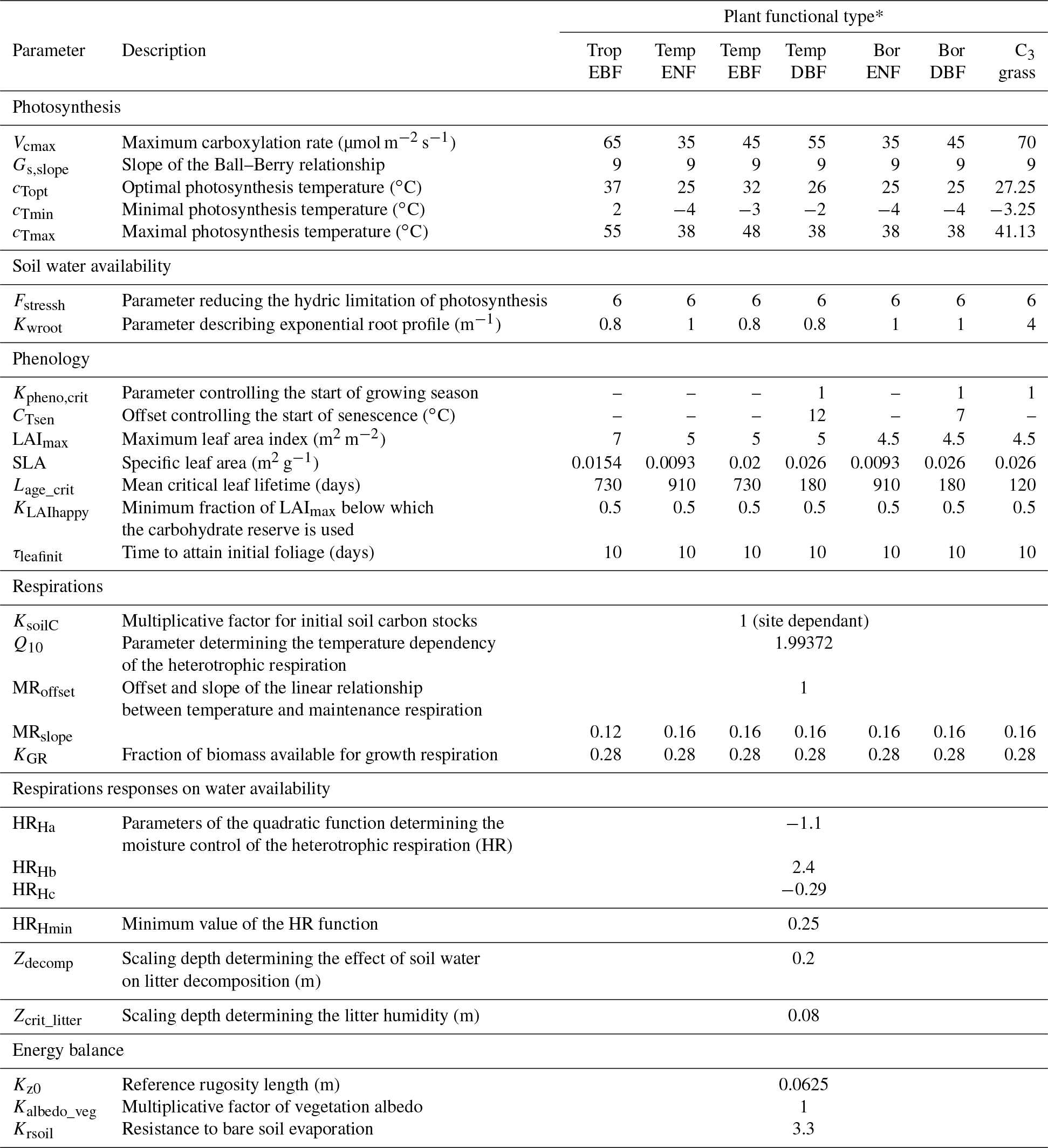
* TropEBF – tropical evergreen broadleaf forest; TempENF – temperate evergreen needleleaf forest; TempEBF – temperate evergreen broadleaf forest; TempDBF – temperate deciduous broadleaf forest; BorENF – boreal evergreen needleleaf forest; BorDBF – boreal deciduous broadleaf forest; C3 grass – C3 grassland.
2.3 Assimilated data: carbon and water fluxes
We use eddy covariance measurements of surface CO2 NEE fluxes and latent heat flux (LE) from the FLUXNET global network (La Thuile database; Baldocchi et al., 2001). Based on an original list of the 252 sites we selected 78 sites, representing 7 PFTs of ORCHIDEE (from the total number of 13) with the number of sites in each PFT varying from 2 (temperate evergreen broadleaf forests, TempEBF) to 24 (C3 grasses) and the length of each observation record varying from 1 to 10 years. We only kept sites where the dominant PFT represents at least 70 % of the footprint of the flux tower so that we could restrict the optimisation to the parameters of one PFT per site. Also, we disregarded sites that had a large discrepancy with respect to the prior ORCHIDEE simulation (in terms of seasonal cycle), which suggests large model structural errors that prevent meaningful parameter optimisations. Note that Peaucelle et al. (2018) explored, with the same model, how to account for plant functional trait variability, refining the PFT distribution. Finally, we only use continuous flux time series that do not contain gaps of more than a few days. This subset of FLUXNET sites corresponds to the one used by Kuppel et al. (2014). The selected sites (geographical location, data period and references) are described in the Supplement (Table S2). Where possible, the LE fluxes have been corrected to close the energy balance, using measurements of the ground heat flux (G) and keeping a constant Bowen ratio to update the latent and sensible heat fluxes (i.e. conservative choice without strong evidence that one turbulent flux may be more impacted than the other one; Twine et al., 2000). Individual days with less than 80 % of data coverage have not been used.
For the assimilation, the half-hourly observations have been averaged on a daily basis and smoothed with a 15-day running mean, following Bacour et al. (2015). This allows us to focus the optimisation on the seasonal and annual timescales, excluding the influence of short-term flux variations. In order to test the influence of smoothing the data on the optimisation performance, preliminary assimilation experiments were run with different smoothing configurations (10-day running mean, 5-day running mean and without smoothing). Overall the choice of the smoothing configuration had little impact on the outcome of this study. A slight decrease in the ability to find the minimum is observed with the gradient-based method when narrowing the smoothing interval for the NEE or LE fluxes. With the random search algorithm the impact is even smaller. The reader is referred to the Supplement for the illustration of the smoothing influence on the fit to the data (Fig. S1, example for TempDBF PFT, last columns). From the results of this test we determined that the key messages of the results are not impacted by the smoothing window; therefore, the results are based on the 15-day running mean.
2.4 Data assimilation framework
2.4.1 The principle of minimisation
The optimisation methodology used in this study relies on a Bayesian statistical formalism (see for instance Tarantola, 2005, Chapter 3). Assuming that the errors associated with the parameters, the observations and the model outputs follow Gaussian distributions, the optimal parameter set corresponds to the minimum of a cost function, J(x), that measures the mismatch between (i) the observations (y) and the corresponding model outputs, H(x), (where H is the model operator), and (ii) the a priori (xb) and optimised parameters (x), weighted by their error covariance matrices:
R and Pb are the prior covariance matrices for the observation and parameter errors, respectively. The error covariance matrices are difficult to assess and thus neglected here, as in most studies (i.e. R and Pb are diagonal). The observation errors (variances) have been defined as the mean-squared difference between the observations and the prior model simulations. This reflects not only the measurement errors but also possibly includes significant model errors. The exact error values assumed for NEE and LE for each site can be found in Tables S3–S4.
As explained in the introduction, two classes of method to minimise the function J(x) are compared; both are described below. Note that using non-Gaussian errors would significantly complicate the application of one class (gradient-based) and is thus out of the scope of this study. MacBean et al. (2016) examined the issues that may arise when using Gaussian assumptions in gradient-based minimisation algorithms; however, they found that the algorithm used in this study could account for quasi non-linearity. Moreover, in the case of ORCHIDEE we have shown in an earlier study (Santaren et al., 2007) that most parameter errors follow Gaussian distributions.
2.4.2 Gradient-based minimisation algorithm
For the gradient-based approach we chose the quasi-Newton algorithm L-BFGS-B to iteratively minimise the cost function (limited memory Broyden–Fletcher–Goldfarb–Shanno algorithm with bound constraints; see Byrd et al., 1995), referred to as BFGS. It was specifically developed for quasi-non-linear optimisation problems and allows for direct assignment of bounds to each parameter.
Each iteration requires the evaluation of the cost function and its gradient with respect to each parameter. Generally, the gradient can be calculated with a finite-difference approximation (i.e. the ratio of the change in model output to the change in model parameter). However, it can be done more precisely using the tangent linear (TL) model (linear derivative of the forward model). For ORCHIDEE the corresponding TL model has been derived with the automatic differentiation tool TAF (Transformation of Algorithms in Fortran; see Giering et al., 2005), following code cleaning and structural adjustments (without changing the physics) to allow the use of TAF (a significant effort that took around 2 years). It was used to calculate the gradient for all parameters except for two phenology parameters, Kpheno,crit and CTsen, associated with threshold functions. For these two parameters, the finite-difference method is more appropriate and was used here.
The search is terminated when the relative change in the cost function becomes smaller than 10−4 during five consecutive iterations. On average the iterative process stopped within 30 iterations. Given that the computation of a TL model run is about twice as long as the standard run of ORCHIDEE, the total computation time for one BFGS optimisation for one site with 30 parameters is equivalent to around 1800 standard model runs.
Gradient-based algorithms have a potential drawback with non-linear models as they are more likely to converge to a local minima of the cost function instead of the global one. In order to assess the extent of this problem we performed a set of independent assimilations starting with 16 different random initial first guesses for the parameter vector, as in Santaren et al. (2014) (see Sect. 2.5).
2.4.3 Random search minimisation algorithm
For the random search approach, we chose the genetic algorithm (GA). The GA is a meta-heuristic optimisation algorithm, belonging to a larger class of evolutionary algorithms that follows the principles of genetics and natural selection (Goldberg, 1989; Haupt and Haupt, 2004). It considers the vector of parameters as a chromosome with each gene corresponding to a given parameter. The algorithm works iteratively, filling a pool of n chromosomes at each iteration. The starting pool is created with randomly perturbed parameters. The chromosomes at each following iteration are created from the randomly chosen chromosomes of the previous iteration by one of the two processes:
-
exchange of the gene sequences of two parental chromosomes (“crossover” process),
-
random perturbation of the selected genes of one parental chromosome (“mutation” process).
The resulting pool is then filled with n best chromosomes from both parental and offspring pools, corresponding to the n lowest cost function values. Furthermore, at each step the chromosomes are ranked in ascending order of the corresponding cost function values and random selection of the new parents is weighted by those ranks in order to guarantee that the best chromosomes produce more descendants (“selection” principle).
The GA performance is sensitive to its particular configuration. In this study, we use the same GA configuration as in Santaren et al. (2014) who tested different GA configurations and chose one, based on computational efficiency (to locate the cost function minimum):
-
number of chromosomes in the pool is 30;
-
number of iterations is 40;
-
crossover/mutation ratio is 4 : 1;
-
number of gene blocks exchanged during crossover is 2;
-
number of genes perturbed during mutation is 1.
For a better convergence of the cost function we reduce the ranges of parameter variations after the 30th iteration by a factor of 0.25 with the centre point at the current best-guess value.
The GA does not require any gradient calculations; therefore, one chromosome rank estimate requires one standard model run and the total computational time for the GA assimilation for one site equals 1200 runs. Contrary to gradient-based methods, random search algorithms allow us to use any form of PDFs for the observation and parameter uncertainties, and thus to use non-Gaussian PDFs.
2.4.4 Posterior uncertainty
Assuming Gaussian prior errors and linearity of the model in the vicinity of the solution, the posterior error covariance matrix of the parameters, A, can be approximated by
where H is the model sensitivity (Jacobian) at the minimum of J(x) (see for instance Tarantola, 1987). From A we can compute error correlations between parameters, a diagnostic that is used to evaluate the information content brought by the observations to discriminate each parameter.
2.5 Numerical experiments and performance metrics
For each data assimilation experiment we performed 16 independent runs, 1 of which has been performed with the standard model parameters as a first guess and the other 15 with different first guesses randomly selected within the range of variation of the parameters. We choose 16 sets based on the available computing resources but we verified, for one case, that increasing this number does not change the overall message. The set of 15 random first guesses was kept identical for all experiments in order to guarantee the same first-guess values. However, for the GA such a procedure is not essential, as the GA relies on a random generation process at each iteration; specific choices related to the random exploration of the parameter space by the algorithm (see Sect. 2.4.3) become crucial and the use of different first guesses is only an additional degree of freedom to explore the parameter space. Both minimisation methods have been tested for two cases: an independent optimisation of the parameters at each site (“single-site” approach, SS) and a simultaneous optimisation of one common set of parameters at all sites belonging to the same PFT (“multi-site” approach, MS).
Overall, we defined the following set of numerical experiments:
-
16 SS assimilation runs for each of the 78 sites that encompass all 7 PFTs with the gradient-based algorithm (BFGS, noted below as SBFGS);
-
16 SS assimilation runs for each of the 78 sites that encompass all 7 PFTs with the GA (SGenetic);
-
16 MS assimilation runs for each of the 7 PFTs with the BFGS algorithm (MBFGS);
-
16 MS assimilation runs for each of the 7 PFTs with the GA (MGenetic).
We address the impact of different first guesses for both the SS and MS optimisations for both methods in each section of the results. Additionally, for one PFT (temperate deciduous broadleaf forest, TempDBF) we performed the same four numerical experiments using pseudo-observations generated from outputs of the model with random parameters, in order to verify if the assimilation methods were finding the correct minima of the cost function. Such pseudo data are not biased by observation uncertainties (no added uncertainties) or model discrepancies, and thus allow us to directly assess the performance and convergence properties of the optimisation schemes. Note that for these pseudo-data experiments the second term of the cost function (Eq. 1) was excluded.
The performances of the optimisation methods are compared using the reduction of the model–data root mean square difference (RMSD) between the prior and the posterior, expressed as %, as well as the range of posterior parameter values and their difference with the true value as estimated from the pseudo-observation tests.
3.1 Model fit to the data
In order to investigate the differences between the minimisation schemes, Fig. 1 presents a comparison of the overall optimisation performances as a summary diagnostic. It displays the prior and median posterior model–data RMSD for all sites used in the study (i.e. the median across the 16 first-guess tests). Additionally, the reader is referred to Fig. S1 in the Supplement for the results obtained at each site for each first guess with the prior and posterior model–data RMSD. We first note that both BFGS and GA successfully optimised the simulated NEE flux (for LE flux, see Fig. S1), significantly reducing the model–data misfit, in line with the results obtained by Kuppel et al. (2014) with the same modelling framework. Below, we first compare the performance of the two methods for the SS (Sect. 3.1.1) and MS (Sect. 3.1.2) cases using global statistics across first-guess tests and we then discuss more quantitatively the benefit of multiple first-guess tests in Sect. 3.1.3.

Figure 1Model–data RMSD for the daily NEE time series at each site grouped by PFT. The prior RMSD values are shown in grey, followed by the median posterior RMSD values obtained within 16 optimisation tests with random first-guess parameter values for each optimisation method. Black horizontal bars show the mean value across the sites for each PFT.
3.1.1 Single site optimisation: comparative performance of the methods (SBFGS vs. SGenetic)
The first objective of the study is to assess which method performs best for a SS optimisation. Figure 2a and b compares the performance of the two methods for all sites in terms of model–data RMSD reduction for the NEE fluxes. The similar comparison for the LE fluxes can be found in the Supplement (Fig. S2). The RMSD reductions are expressed in percentage; they correspond to the median value (left plots) and the 5th–95th percentile range (R90; right plots) across the 16 random first-guess tests.
At all sites of all PFTs the SS GA (SGenetic) provides better fit to the data (median across all 16 first-guess tests) than the SS gradient-based algorithm (SBFGS), with only a few exceptions (see Figs. S1 and 2a). The SGenetic leads up to 40 % of additional model–data RMSD reduction compared to the SBFGS algorithm, with a mean improvement across all sites of 10 %. In most cases the worst posterior RMSD value achieved with the SGenetic algorithm is better than the median value for the SBFGS method. The SBFGS approach is slightly better only at eight sites with no more than 4 % of additional RMSD reduction.
The spread of the results obtained with the use of different first-guess parameters (16 tests) is also much lower for the SGenetic compared to the SBFGS method, for nearly all sites (Fig. 2b). On average the R90 values are 3.6 times lower with the GA – the SGenetic method is only slightly disadvantageous for 3 sites out of 78, although the spread across the 16 first guesses remains low (<10 %). Overall, the mean spread of the RMSD reduction for the SGenetic case is around 10 %. This clearly indicates that the GA, following the set up described in Sect. 2.4.3, is able to find nearly the same minimum of the cost function independently from the choice of the first-guess parameters (with a significant improvement of the model–data misfit, see Fig. 1). On the contrary, the results of the SBFGS method are highly dependent on the first-guess model parameters, with a spread above 22 % for half of the sites. Finally, if we compare the best achieved RMSD reduction within the 16 first-guess tests (see Tables S3 and S4 in the Supplement), we obtain similar performances for most of the sites of 5 PFTs out of 7, excluding TropEBF and BorDBF, where the SGenetic method still produces better results than the SBFGS method.
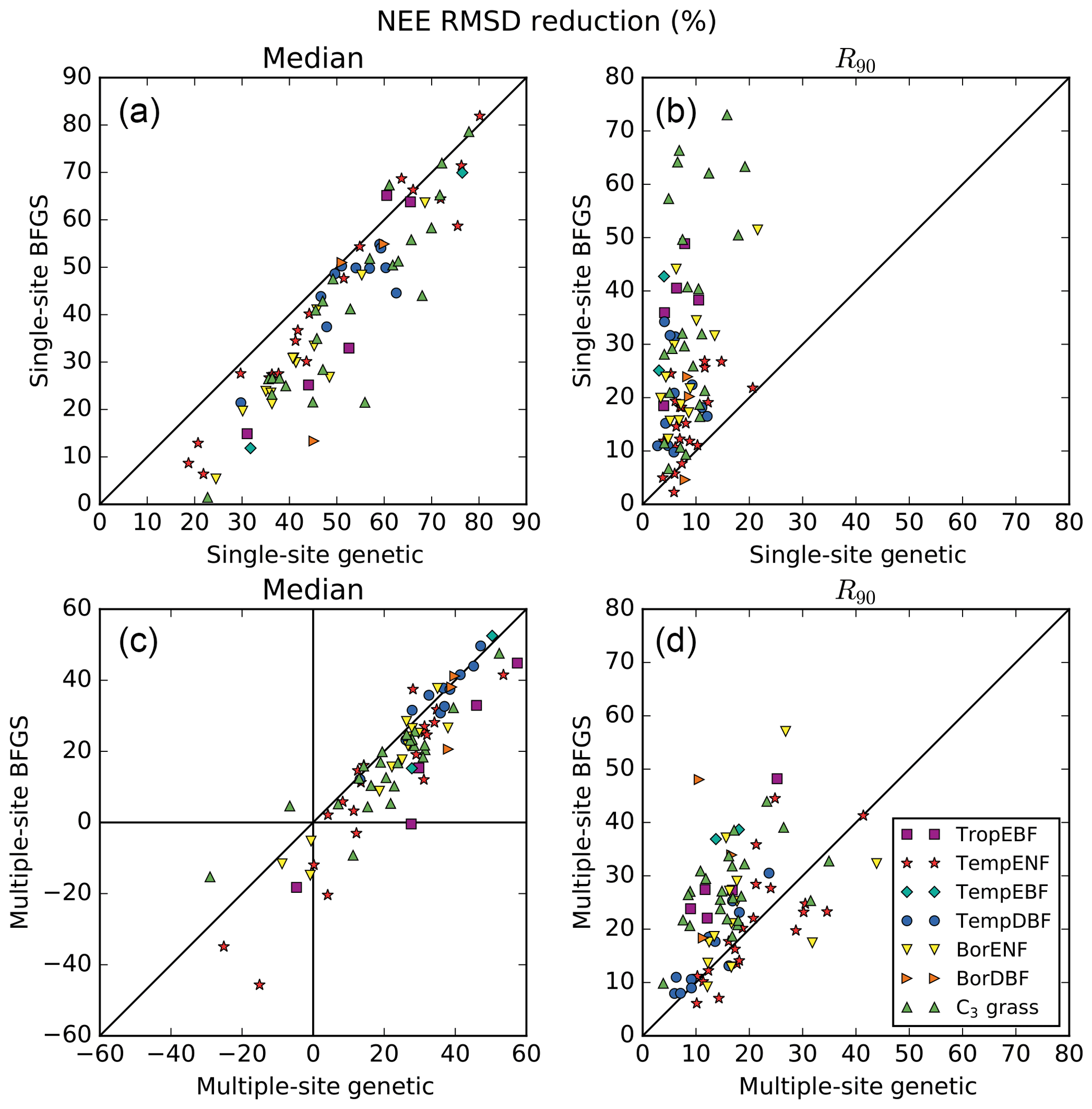
Figure 2Comparison of the performances between the gradient-based and genetic methods in terms of model–data RMSD reduction (%) obtained for the daily NEE fluxes. The left panels show the medians from the results obtained within 16 optimisation tests with random first-guess parameter values for each site; the right panels show the spreads between the 5th and 95th percentiles (R90) of the same distributions.
With the gradient-based method (SBFGS), using the standard ORCHIDEE model parameters as a first guess does not guarantee an optimal reduction of the cost function – the corresponding posterior RMSD could be either the lowest or the highest one of the 16 tests (these cases are shown by a circle, as opposed to a cross, in Fig. S1 that displays the posterior RMSD for all sites and all 16 tests). Although we have used the same random parameter sets for each site of a given PFT, the “optimal” first-guess parameter set (i.e. the one providing the largest cost function reduction) differs between sites. It indicates that the shape of the cost function varies between sites and that there is no optimal prior first guess with the SBFGS gradient method, which is prone to getting caught in local-minima if the assumption of model quasi-linearity is not met. Overall, this highlights one weakness of gradient-based methods and the need to perform several independent assimilations starting from different first-guess parameter values (see Sect. 3.1.4).
3.1.2 Multi-site optimisation: comparative performances of the methods (MBFGS vs. MGenetic)
The reduction in NEE RMSD for the MS optimisations (MBFGS for the gradient-based method and MGenetic for the Genetic algorithm) is illustrated in Fig. 2c, d. First, the MS optimisations provide lower RMSD reduction than the SS optimisations (Fig. 2a, b vs. c, d). This is the trade-off between fitting a specific site versus fitting an ensemble of sites representing more accurately the diversity of plant, soil and climate for a given PFT. We then notice that for few sites the RMSD is increasing after the optimisation (i.e. negative value of the RMSD reduction): 1 site for TropEBF and C3 grass PFTs and 3 sites for TempENF and BorENF. On average these sites have only 1 or 2 years of data with large prior observation errors and thus a smaller weight in the cost function compared to the other sites of the same PFT. This could thus explain that the optimisation degrades the model-data fit at these sites but it could also indicate that there is no optimal parameter set improving the model-data fit at all sites, suggesting the need to refine the PFT description and/or to improve the model structure (see a list of potential impacts of missing processes in the ORCHIDEE model in Sect. 2.1). Note that MS optimisations are likely to be more impacted by model structural errors than SS optimisation, as these errors may have different impacts at each site. Limits arise when the objective is to study the response of a specific ecosystem (and not a generic PFT) to external drivers as the MS parameter set might be suboptimal.
The performance of the two methods differs between the PFTs. For TropEBF, TempENF and C3 grass PFTs the GA still provides on average significantly larger RMSD reduction than the gradient method, with ratios between the two of 2.0, 1.8 and 1.4, respectively. For the other four PFTs both methods show much smaller differences and for TempDBF the average RMSD reduction is exactly the same. Overall, at 50 sites (from 78) the MBFGS method provides performances comparable to the MGenetic method (RMSD reductions differ by less than 25 %) or even slightly better (see Tables S3/S4 in the Supplement for all numbers) and the mean additional RMSD reduction for the MGenetic method is only 6 %.
The spread across random first guesses between the two methods is much more comparable than for the SS optimisations. The R90 values for the gradient-based method are only considerably larger for half of the sites than the GA method (with values up to 2 times larger), except for two PFTs (TempENF and TempDBF) where they are similar on average (Fig. 2d). This suggests that increasing the number of observations and/or capturing a greater range of sensitivity to the parameters acts to linearise or smooth the cost function, thereby ensuring that the gradient-based method does not get as caught in local minima as in the SS optimisations.
The last point to notice is that using the standard ORCHIDEE parameter set as a first guess with the MBFGS method always leads to significant improvement of the model-data fit (see Fig. S1) with RMSD reduction at the same level as the median RMSD reduction for the MGenetic method. This was not the case for the SS optimisation (see Sect. 3.1.1). With a MS optimisation the gradient-based scheme is less dependent on the first guess, likely due to the smoothing of the cost function as discussed above and therefore performing several random first-guess tests is less needed. Overall for the MS optimisations the choice of the minimisation algorithm seems thus less crucial than for the SS cases.
Nonetheless, the MS method conceals certain limitations. The optimisation may not perform well (i.e. not lead to a large minimisation of the cost function) if the different sites have very different behaviours in terms of the carbon and water cycle responses to climate forcing. This case points to the need to reconsider the PFT geographical description with possible further regional split; it is suggested for TropEBF and C3 grass PFTs. Additionally, MS optimisations, that requires large computing time, are more complicated to set up, with the need to have coherent observation errors between sites. We need to avoid that one or few sites dominate the cost function because of a too low observation error (measurement and model errors grouped in the R term) and thus prevent the optimisation to fit all the other sites.
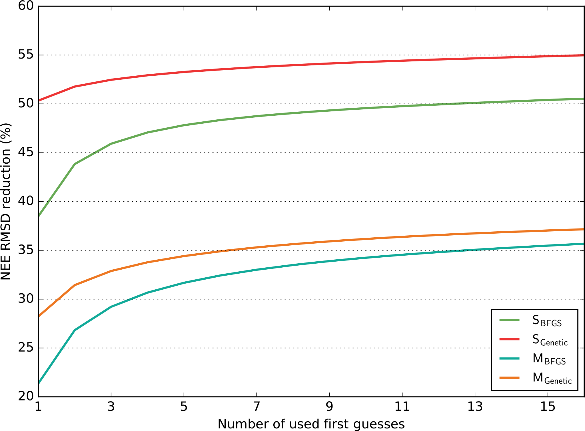
Figure 3Model–data RMSD reduction (in %) obtained for the NEE fluxes as a function of the number of runs performed with random first-guess parameter values (for each configuration, SBFGS, SGenetic, MBFGS and MGenetic). For each number of first guesses (x axis) all possible combinations across the 16 optimisation tests (i.e. 16 first guesses) are considered and the maximum RMSD reductions are calculated; the mean of these maxima is reported on the y axis. The results are averaged across all sites for each configuration.
3.1.3 Benefit of multiple first guesses for a gradient-based approach
We now investigate more quantitatively the benefit of using several first-guess tests (16), especially for the gradient-based algorithm (see Sect. 2.5).
In order to analyse the influence of the number of first-guess tests on the optimisation performance, for each configuration we bin the 16 first-guess optimisations in all possible groups of n elements and defined for each group the maximum RMSD reduction. We then take the mean values of all these maxima. The results are shown in Fig. 3 for all configurations (SBFGS, SGenetic, MBFGS and MGenetic) as a function of the number of first guesses (n) for the NEE fluxes (with the similar results in Appendix, Fig. S3 for the LE fluxes). Only the mean across all PFTs is displayed and analysed. This illustrates the gain of adding more first-guess tests in the different configurations.
On average for the SS configurations, the GA (SGenetic) with any number of first guesses leads to 50.5–55 % of RMSD reduction for the NEE fluxes; the increase in RMSD reduction between 1 and 16 first guesses is small (≈4 %). However, the gradient-based method (SBFGS) needs 15 independent first-guess optimisations in order to reach the same level of RMSD reduction as with one first guess of SGenetic and there is a substantial increase in the RMSD reduction from one to five first guesses (≈9 %), while the improvement afterward is much smaller. For the SGenetic method, the increase in the RMSD reduction is only significant from one to two first-guess tests.
For the MS configurations, the performances of the gradient-based method are more similar to that of the GA (although both with smaller RMSD reduction, as discussed in the previous section). On average, the MBFGS method needs three first-guess tests to reach the performance of the MGenetic method obtained with one test. Like with the SS configuration the increase in the RMSD reduction is substantial for the MBFGS method between 1 and 5 first guesses (≈10 %) and much smaller afterwards.
Overall this analysis highlights that using several first guesses is crucial for the gradient-based method and that at least 3 to 5 tests are required to obtain a RMSD within 5 % of the optimal value obtained with 16 tests (for both SBFGS and MBFGS). The GA is much less sensitive to the number of first-guess tests performed. Using a MS configuration reduces the difference between the two algorithms and requires less random first-guess tests for the MBFGS method to achieve performances comparable to the MGenetic method. Note finally that increasing the number of first-guess tests to much larger values would lead to a convergence of the method performances.
3.2 Estimated parameter values
We now investigate how the choice of the minimisation method impacts the retrieved parameters. We only discuss the results of one PFT, temperate deciduous broadleaf forest (TempDBF), for a more in-depth investigation. We obtained similar findings for the other PFTs (see Fig. S4 in the Supplement). We selected TempDBF given that the RMSD reduction for this PFT is significant and that it includes a large number of sites (11). Before investigating the standard optimisations with real data, we discuss the results of the pseudo-observation experiments (see Sect. 2.5) in order to analyse the ability of the different methods to retrieve “true” parameter values.
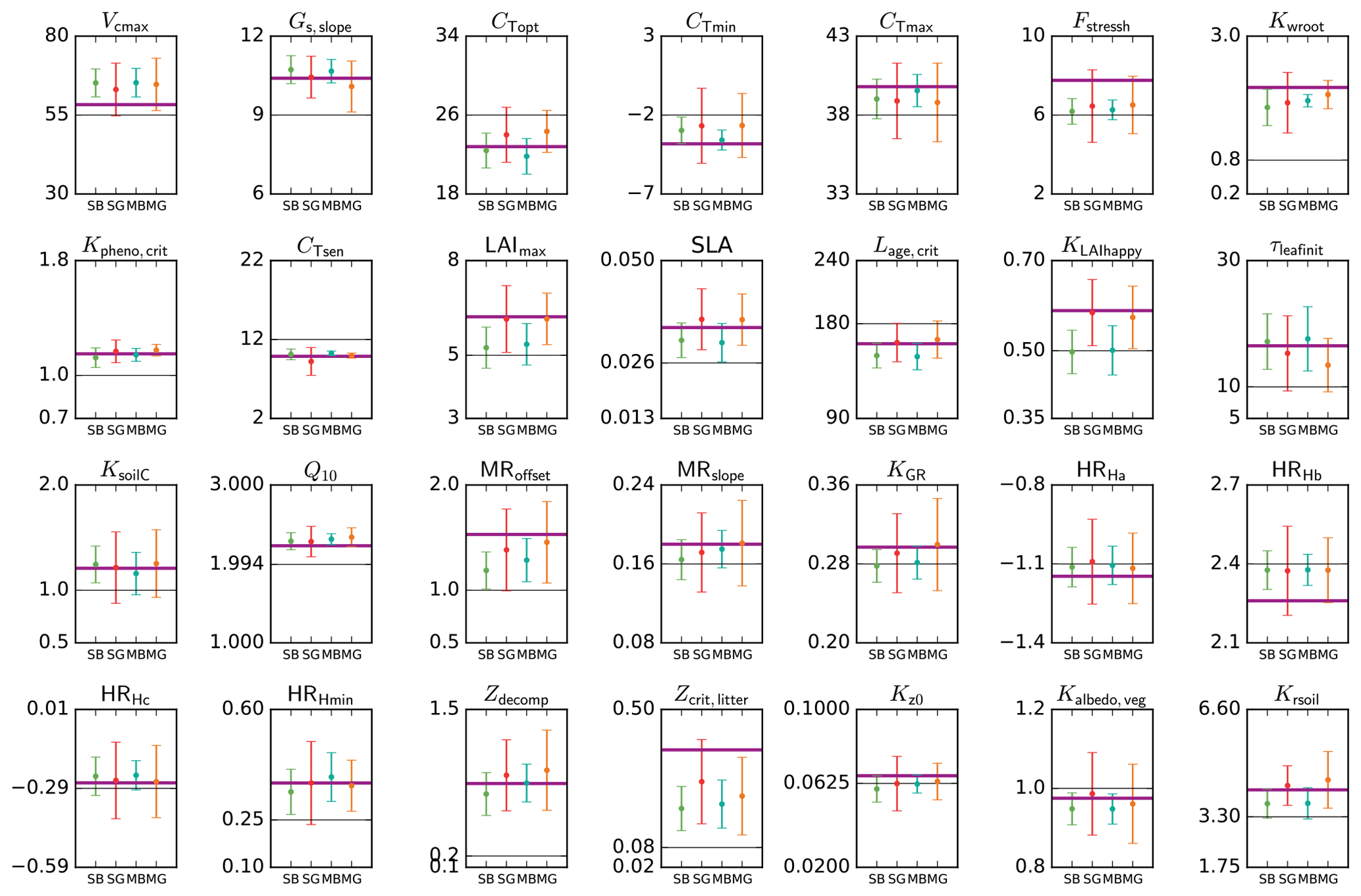
Figure 4Parameter estimates from a pseudo-data experiment for the temperate deciduous broadleaf forest PFT. Results for the four different methods (SBFGS, SB; SGenetic, SG; MBFGS, MB; and MGenetic, MG) are displayed: mean value and standard deviation across 16 random first-guess tests. The thick horizontal purple lines correspond to the “true” parameter values (defined randomly); the thin grey horizontal lines correspond to the prior value, which is equal to the default ORCHIDEE model value. The vertical axis limits represent the range of parameter variation.
3.2.1 Estimating the correct posterior parameter value – pseudo-observation experiments
Figure 4 shows the estimated parameter values, the standard prior values and the “true” values for the pseudo-observation experiments with TempDBF. We display the mean and standard deviation across the 16 first-guess tests and for the SS assimilations we take the mean across all sites.
On average both BFGS and GA are not able to retrieve exactly the true value for all parameters (i.e. values used to generate the pseudo data), although many of the parameters are relatively well estimated by the optimisation schemes. Out of 28 parameters, on average across all methods and all first guesses, 14 have posterior values that are within 5 % of the true value, using the physical parameter range to define the percentage (i.e. true value ±5 % of the allowed range of variation); 6 parameters are between 5 and 10 %; 7 between 10 and 20 %, and 1 parameter (Zcrit,litter) is 29 % from the true value. These differences are mainly related to differences in the sensitivity of the model outputs (NEE and LE) with respect to the different parameters (with lower sensitivity for Zcrit,litter). The most constrained parameters (5 % range with the small deviation around true value) are Gs,slope, cTopt, Kpheno,crit, CTsen, Lage,crit, τleafinit, KsoilC and Q10. We can thus expect more robust results with these parameters using real data. However, the uncertainties associated to the real data, and the fact that these uncertainties may not be adequately described in the observation error covariance matrix, will complicate the parameter retrieval (see MacBean et al., 2016). Note that for many other parameters the error bars (standard deviation across all first-guess tests) encompass the true values (Vcmax, cTmin, cTmax, SLA, KGR, MRoffset, MRslope, HRHc, HRHmin, Zdecomp, Kalbedo,veg, Krsoil).
As it was already outlined in Santaren et al. (2014), the differences obtained between the true and optimised parameter values are likely due to equifinality problems (i.e. multiple solutions achieving the same overall global minimum of the cost function) or the existence of local minima where the algorithm is trapped. These issues vary between parameters and are related to the sensitivity of the model outputs to each parameter, the prior parameter uncertainty and the level of error correlation between parameters. Existing correlations and anti-correlations between the impacts of different parameters prevents from retrieving all of them with the chosen set of observations (daily means of NEE and LE) and the optimisation frameworks that are used.
Differences between the methods exist but are not systematic. There are a few parameters that perform well only with one of the methods, both for SS and MS optimisations. For example, cTopt, τleafinit and Zdecomp are correctly estimated with only the gradient-based approach. On the contrary, the generic algorithm performs much better for parameters like LAImax, SLA, Lage,crit, KLAIhappy and Krsoil. A few parameters are not well estimated by both methods, like Fstressh, HRHb and Zcrit,litter, having the largest difference with respect to the true value. The estimated errors (Eq. 2) associated to these poorly retrieved parameters are relatively large, and for Fstressh and HRHb they are highly correlated with other parameters; we should thus be very cautious when interpreting their value with real data optimisations. Overall, we observe that 19 parameters out of 28 are better estimated on average by the GA (SGenetic, MGenetic) than by the gradient-based method (SBFGS, MBFGS). This is coherent with the results of the fit to the data (Sect. 3.1), indicating that the gradient method is more likely stuck in local minima than the GA.
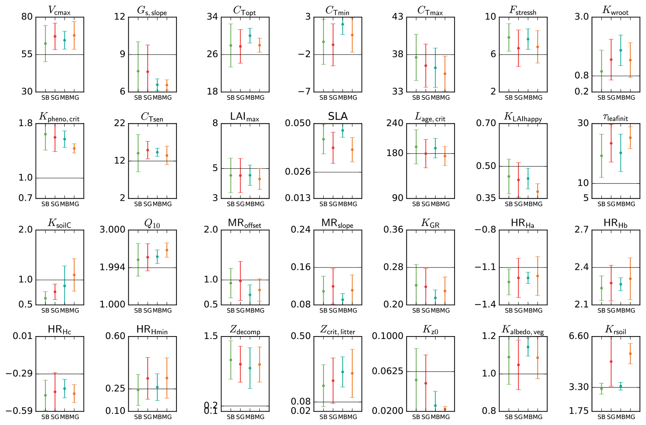
Figure 5Mean posterior model parameter values for temperate deciduous broadleaf forest PFT. Results for the four different methods (SBFGS, SB; SGenetic, SG; MBFGS, MB; and MGenetic, MG) are displayed: mean value and standard deviation across 16 random first-guess tests. Grey horizontal lines represent prior values, which are equal to the default ORCHIDEE model values. The vertical axis limits represent the range of parameter variation.
3.2.2 Spread in parameter values across methods and first-guess tests – real data experiments
Using real data, Fig. 5 displays the mean posterior estimates of the TempDBF parameters across all first-guess tests for the four optimisation methods (SBFGS, SGenetic, MBFGS and MGenetic). For most of the parameters the mean optimised values are relatively similar between the BFGS and the GAs, with some exceptions. Twelve parameters (Gs,slope, cTopt, cTmin, Kpheno,crit, CTsen, LAImax, KLAIhappy, Q10, MRoffset, KGR, HRHc, Kz0) out of 28 show posterior differences between SGenetic and SBFGS methods that are lower than 5 % of the physical range for each parameter, while 7 (cTmax, Fstressh, Kwroot, SLA, τleafinit, HRHmin, Kalbedo,veg) show differences between 10 and 20 %, whereas Krsoil goes up to 36 %. For MGenetic and MBFGS methods, only 7 parameters are within the 5 % variation range (Gs,slope, CTsen, LAImax, Kz0 as for the SS approaches, plus HRHa, Zdecomp, Zcrit,litter), and 14 parameters have differences over 10 % (same list as for the SS methods excluding cTmax, plus cTopt, cTmin, Kpheno,crit, Lage,crit, KLAIhappy, KsoilC and MRslope). Note that most parameters that are well constrained (i.e. small spread across the optimisation methods) also correspond to the most constraint ones in the pseudo-observation experiments (like Gs,slope, cTopt, Kpheno,crit, CTsen, Q10, HRHc). However, few parameters demonstrate different behaviour between the real and pseudo-data tests (like KLAIhappy, MRoffset, LAImax).
For certain parameters (cTopt, LAImax, SLA, Lage,crit, KLAIhappy, KGR, Krsoil) we obtain significant differences in the estimated values between BFGS and GA, for both SS and MS cases. Whereas the gradient-based methods looks for the optimal parameter set in the vicinity of the first-guess set-up, the random search algorithm may jump to a completely different parameter state during one iteration. Given that with pseudo-data the GA manages to find the true values for these parameters much more precisely than the BFGS, we can speculate that the GA provides more optimal posterior estimates in the real data experiments as well.
Another feature is that for the SS and the MS cases, both algorithms (BFGS and GA) lead, for most parameters, to a similar dispersion of the posterior estimates from the ensemble of 16 first guesses (see Fig. 5). However, for some parameters (Fstressh, SLA, MRoffset, MRslope, HRHa, HRHb, HRHc, HRHmin, Zcrit,litter, Kalbedo,veg, Krsoil) the GA method gives, surprisingly, much higher distribution of the posterior values. It corresponds to the parameters that have also not been correctly estimated in the pseudo-observation tests (see Sect. 3.2.1) with estimated value outside the 10 % range around the true value. Although not intuitive, the random sampling over the parameter space with the GA could explain that for each first guess the GA method may end up exploring a larger domain of the parameter space and thus converge to more different parameter sets than the gradient-based method.
For each parameter, the dispersion obtained with the different first guesses is lower for the MS case compared to the SS case, for both algorithms. On average the mean dispersion for the SS approaches is 25 % of the parameter range (with minimum and maximum spreads of 7.3 % and 42 %, respectively), and for the MS approaches it is only 14 % (between 3.4 % and 32 %). This reflects that with the MS approach the shape of the cost function is more smooth due to the combination of different NEE/LE responses to the parameter variations (differences induce mainly by different climate, soil type and plant species), which in turns facilitate the convergence to the global minimum. For the SS case, the shape of the cost function may significantly differ between sites leading to a larger parameter spread in response to multiple first guesses (compared to the MS case). This is specifically illustrated with the parameters Kwroot, CTsen, Q10, HRHa, HRHb and Kz0. The only exception is for KsoilC, a parameter that is specific to each site even in the MS approach (see Sect. 2.2).
Throughout this study, we compared the performances of two algorithms for the optimisation of the ORCHIDEE land surface model (LSM) parameters. The two algorithms belong to two different classes of method; the L-BFGS-B algorithm is a gradient-based method and the genetic algorithm (GA) is a global random search method. The two methods were used to optimise 28 parameters (16 of which are PFT-dependent), using daily NEE and LE fluxes from 78 eddy covariance flux measurement sites. Both methods were run either independently at each site (single-site, SS, approach) or simultaneously at all sites for each PFT (multiple-site, MS, approach). For each configuration we ran 16 different tests in which the prior parameter values are selected randomly. The main findings are the following.
-
For the single site (SS) optimisations, the random search algorithm (GA) results in lower values of the posterior cost function than the gradient-based method (BFGS) for nearly all sites.
-
The difference between results derived from the GA and BFGS methods are smaller for MS optimisations than at SS. We suggest that smaller difference between GA and BFGS for MS optimisations is due to a smoothing of the cost function shape in the MS optimisations given a greater number of observations are included in the assimilation.
-
The GA results in a closer approximation of the true posterior parameter value than BFGS with the pseudo-observation tests, for both the SS and MS experiments.
-
When performing the same optimisation with multiple first guesses in parameter space (16 random first guesses), the spread in posterior cost function value is much larger for the BFGS than the GA methods for SS optimisations, due to the higher likelihood that gradient-based methods get stuck in local minima. The spread in posterior cost function value from 16 first guesses is closer for the MS optimisations, although still higher for the BFGS than the GA methods. Again, we suggest this is because the cost function is smoother in MS optimisations; therefore, the BFGS algorithm is less likely to get stuck in local minima.
-
If using the BFGS method, our results suggest that performing the same tests with several first guess parameters may ensure a reduction of the cost function that is comparable to the one obtained with the random search GA method. This is important, because running a random search method may be computationally unfeasible for some modelling groups; therefore, the BFGS method can be used as a reliable alternative, provided a number of first-guess parameters are used.
The computing cost of the BFGS and GA algorithms were on average relatively similar, when considering all experiments, although slightly higher for the BFGS algorithm. With BFGS, the cost depends on which iteration the convergence criterion is met (see Sect. 2.4.2). For the random search GA method, the value of the cost function may be further decreased by increasing the number of iterations (currently at 40). We choose a set-up for the random search method that led to similar computing cost than the gradient-based method, but this could be revised depending on the cost of a SS model simulation (currently around 20–30 s with ORCHIDEE for 1 year using one standard processor depending on the number of output variables).
Most of the differences between the BFGS and GA algorithms are related to the shape of the cost function, in part controlled by the non-linearity of the model. Our results can thus be extrapolated to other LSMs, provided that they have similar complexity and level of non-linearity. With SS optimisations, we advise to use a random search method – the GA being just one possibility. If a gradient-based method is preferred, we strongly recommend performing at least several tests using different random first-guess parameter values. Our study suggests that for the chosen model and inversion set-up we should use at least 5 tests; however, this number will depend on the model complexity and particular set up of the DA experiment (e.g. type and number of observations included in the assimilation).
With MS optimisations, the use of a gradient-based method is less critical, due to a smoother cost function with the addition of observations from many sites. In this case, pseudo-data experiments, with known true parameter values, help to assess the strength of the method with the selected model and observations. They reveal how many, and which, parameters are likely to be poorly constrained because of the existence of local minima and/or a broad flat minimum of the cost function. Finally, note that with a random search method, we can use any assumption for the PDF of the prior observation or parameter uncertainties.
The results obtained in this study with eddy covariance flux measurements are likely to hold with other, site-specific, in situ or remote-sensing observations (satellite vegetation activity data, carbon pool measurements, etc.); although similar investigations are needed to precisely quantify the differences between methods for other types of observations. On the other hand, using global simulations (i.e. all grid cells) is likely to produce smoother cost functions and thus to favour gradient-based methods, at least from a computational point of view (especially if an adjoint model is available to efficiently derive the gradient of the cost function with respect to all parameters). This is illustrated in Ziehn et al. (2012) with the assimilation of atmospheric CO2 data in BETHY LSM. Additional studies to characterise the level of smoothness of the cost function as a function of model complexity, data types and approach (from SS to global optimisation) would nevertheless be beneficial and provide additional practical guidance to modelers carrying out DA experiments in their choice of parameter optimisation method.
The ORCHIDEE model code and the run environment are open source and available at https://orchidee.ipsl.fr (last access: 26 November 2018). The tangent linear version of the ORCHIDEE model has been generated using commercial software (TAF; http://www.fastopt.com/products/taf, last access: 26 November 2018), thus only the “forward” version of the ORCHIDEE model is available for sharing. The optimisation tool is available through a dedicated web site for data assimilation with ORCHIDEE (https://orchidas.lsce.ipsl.fr, last access: 26 November 2018). Nevertheless readers interested in running ORCHIDEE and/or optimisation tool are encouraged to contact the corresponding author for full details and latest bug fixes.
The supplement related to this article is available online at: https://doi.org/10.5194/gmd-11-4739-2018-supplement.
PP initially designed the study with further contribution from all co-authors. CB, DS and VB have developed the data assimilation code: CB mainly focused on the gradient-based method, DS on the genetic algorithm and VB on the consolidation of the two versions into a single stand-alone tool. SK worked on the multi-site method implementation and on the input data. VB performed all simulations. VB, NM, PP and CB analysed and synthesised the results. VB, NM and PP mainly contributed to the text.
This work used eddy covariance data acquired by the FLUXNET community and in particular
by the following networks: AmeriFlux (U.S. Department of Energy, Biological and
Environmental Research, Terrestrial Carbon Program; DE-FG02-04ER63917 and
DE-FG02-04ER63911), AfriFlux, AsiaFlux, CarboAfrica, CarboEuropeIP, CarboItaly,
CarboMont, ChinaFlux, Fluxnet-Canada (supported by CFCAS, NSERC, BIOCAP, Environment
Canada, and NRCan), GreenGrass, KoFlux, LBA, NECC, OzFlux, TCOS-Siberia and USCCC. We
acknowledge the financial support to the eddy covariance data harmonisation provided by
CarboEuropeIP, FAO-GTOS-TCO, iLEAPS, Max Planck Institute for Biogeochemistry, National
Science Foundation, University of Tuscia, Universiteì Laval, Environment Canada and US
Department of Energy and the database development and technical support from Berkeley
Water Center, Lawrence Berkeley National Laboratory, Microsoft Research eScience, Oak
Ridge National Laboratory, University of California – Berkeley and the University of
Virginia.
Edited by: David Lawrence
Reviewed by: two anonymous referees
Anav, A., Friedlingstein, P., Kidston, M., Bopp, L., Ciais, P., Cox, P., Jones, C., Jung, M., Myneni, R., and Zhu, Z.: Evaluating the land and ocean components of the global carbon cycle in the CMIP5 earth system models, J. Climate, 26, 6801–6843, https://doi.org/10.1175/JCLI-D-12-00417.1, 2013.
Bacour, C., Peylin, P., MacBean, N., Rayner, P. J., Delage, F., Chevallier, F., Weiss, M., Demarty, J., Santaren, D., Baret, F., Berveiller, D., Dufrêne, D., and Prunet, P.: Joint assimilation of eddy-covariance flux measurements and FAPAR products over temperate forests within a process-oriented biosphere model, J. Geophys. Res.-Biogeosci., 120, 1839–1857, 2015.
Baldocchi, D., Falge, E., Gu, L., Olson, R., Hollinger, D., Running, S., Anthoni, P., Bernhofer, C., Davis, K., and Evans, R.: FLUXNET: a new tool to study the temporal and spatial variability of ecosystem-scale carbon dioxide, water vapor, and energy flux densities, B. Am. Meteorol. Soc., 82, 2415–2434, 2001.
Braswell, B. H., Sacks, W. J., Linder, E., and Schimel, D. S.: Estimating diurnal to annual ecosystem parameters by synthesis of a carbon flux model with eddy covariance net ecosystem exchange observations, Global Change Biol., 11, 335–355, 2005.
Byrd, R. H., Lu, P., Nocedal, J., and Zhu, C.: A limited memory algorithm for bound constrained optimization, SIAM J. Sci. Comput., 16, 1190–1208, 1995.
Chorin, A. J. and Morzfeld, M.: Conditions for successful data assimilation, J. Geophys. Res.-Atmos., 118, 11522–11533, https://doi.org/10.1002/2013JD019838, 2013.
Cramer, W., Bondeau, A., Woodward, F. I., Prentice, I. C., Betts, R. A., Brovkin, V., Cox, P. M., Fisher, V., Foley, J. A., Friend, A. D., Kucharik, C., Lomas, M. R., Ramankutty, N., Sitch, S., Smith, B., White, A., and Young-Molling, C.: Global response of terrestrial ecosystem structure and function to CO2 and climate change: results from six dynamic global vegetation models, Global Change Biol., 7, 357–373, https://doi.org/10.1046/j.1365-2486.2001.00383.x, 2001.
Dietze, M. C., Lebauer, D. S., and Kooper, R.: On improving the communication between models and data, Plant Cell Environ, 36, 1575–1585, https://doi.org/10.1111/pce.12043, 2013.
Ducoudré, N. I., Laval, K., and Perrier, A.: SECHIBA, a new set of parameterizations of the hydrologic exchanges at the land atmosphere interface within the LMD atmospheric general circulation model, J. Climate, 6, 248–273, 1993.
Dufresne, J.-L., Foujols, M.-A., Denvil, S., Caubel, A., Marti, O., Aumont, O., Balkanski, Y., Bekki, S., Bellenger, H., Benshila, R., Bony, S., Bopp, L., Braconnot, P., Brockmann, P., Cadule, P., Cheruy, F., Codron, F., Cozic, A., Cugnet, D., de Noblet, N., Duvel, J.-P., Ethé, C., Fairhead, L., Tichefet, T., Flavoni, S., Friedlingstein, P., Grandpeix, J.-Y., Guez, L., Guilyardi, E., Hauglustaine, D., Hourdin, F., Idelkadi, A., Ghattas, J., Joussaume, S., Kageyama, M., Krinner, G., Labetoulle, S., Lahellec, A., Lefebvre, M.-P., Lefevre, F., Levy, C., Li, Z. X., Lloyd, J., Lott, F., Madec, G., Mancip, M., Marchand, M., Masson, S., Meurdesoif, Y., Mignot, J., Musat, I., Parouty, S., Polcher, J., Rio, C., Schulz, M., Swingedouw, D., Szopa, S., Talandier, C., Terray, P., Viovy, N., and Vuichard, N.: Climate change projections using the IPSL-CM5 Earth System Model: from CMIP3 to CMIP5, Clim. Dynam., 40, 2123–2165, https://doi.org/10.1007/s00382-012-1636-1, 2013.
Field, C. B. and Raupach, R. M.: The Global Carbon Cycle: Integrating Humans, Climate, and the Natural World, Island Press, Washington, 2004.
Fox, A., Williams, M., Richardson, A. D., Cameron, D., Gove, J. H., Quaife, T., Ricciuto, D., Reichstein, M., Tomelleri, E., Trudinger, C. M., and Van Wijk, M. T.: The REFLEX project: comparing different algorithms and implementations for the inversion of a terrestrial ecosystem model against eddy covariance data, Agr. Forest Meteorol., 149, 1597–1615, https://doi.org/10.1016/j.agrformet.2009.05.002, 2009.
Friedlingstein, P., M. Meinshausen, V. K. Arora, C. D. Jones, A. Anav, S. K. Liddicoat, and R. Knutti.: Uncertainties in CMIP5 Climate Projections due to Carbon Cycle Feedbacks, J. Climate, 27, 511–526, https://doi.org/10.1175/jcli-d-12-00579.1, 2014.
Giering, R., Kaminski, T., and Slawig, T.: Generating efficient derivative code with TAF, Fut. Gen. Comp. Syst., 21, 1345–1355, https://doi.org/10.1016/j.future.2004.11.003, 2005.
Goldberg, D.: Genetic Algorithms in Search, Optimization and Machine Learning, Addison-Wesley, 1989.
Groenendijk, M., Dolman, A. J., van der Molen, M. K., Leuning, R., Arneth, A., Delpierre, N., Gash, J. H. C., Lindroth, A., Richardson, A. D., Verbeeck, H., and Wohlfahrt, G.: Assessing parameter variability in a photosynthesis model within and between plant functional types using global Fluxnet eddy covariance data, Agr. Forest Meteorol., 151, 22–38, https://doi.org/10.1016/j.agrformet.2010.08.013, 2011.
Haupt, R. L. and Haupt, S. E.: Practical Genetic Algorithms, John Wiley & Sons, 2004.
Kato, T., Knorr, W., Scholze, M., Veenendaal, E., Kaminski, T., Kattge, J., and Gobron, N.: Simultaneous assimilation of satellite and eddy covariance data for improving terrestrial water and carbon simulations at a semi-arid woodland site in Botswana, Biogeosciences, 10, 789–802, https://doi.org/10.5194/bg-10-789-2013, 2013.
Krinner, G., Viovy, N., de Noblet-Ducoudré, N., Ogée, J., Polcher, J., Friedlingstein, P., Ciais, P., Sitch, S., and Prentice, I. C.: A dynamic global vegetation model for studies of the coupled atmosphere-biosphere system, Global Biogeochem. Cy., 19, GB1015, https://doi.org/10.1029/2003GB002199, 2005.
Kuppel, S., Peylin, P., Chevallier, F., Bacour, C., Maignan, F., and Richardson, A. D.: Constraining a global ecosystem model with multi-site eddy-covariance data, Biogeosciences, 9, 3757–3776, https://doi.org/10.5194/bg-9-3757-2012, 2012.
Kuppel, S., Peylin, P., Maignan, F., Chevallier, F., Kiely, G., Montagnani, L., and Cescatti, A.: Model–data fusion across ecosystems: from multisite optimizations to global simulations, Geosci. Model Dev., 7, 2581–2597, https://doi.org/10.5194/gmd-7-2581-2014, 2014.
Luo, Y., Ahlström, A., Allison, S.D., Batjes, N.H., Brovkin, V., Carvalhais, N., Chappell, A., Ciais, P., Davidson, E. A., Finzi, A., and Georgiou, K.: Toward more realistic projections of soil carbon dynamics by Earth system models, Global Biogeochem. Cy., 30, 40–56, 2016.
MacBean, N., Maignan, F., Peylin, P., Bacour, C., Bréon, F.-M., and Ciais, P.: Using satellite data to improve the leaf phenology of a global terrestrial biosphere model, Biogeosciences, 12, 7185–7208, https://doi.org/10.5194/bg-12-7185-2015, 2015.
MacBean, N., Peylin, P., Chevallier, F., Scholze, M., and Schürmann, G.: Consistent assimilation of multiple data streams in a carbon cycle data assimilation system, Geosci. Model Dev., 9, 3569–3588, https://doi.org/10.5194/gmd-9-3569-2016, 2016.
Moore, D. J., Hu, J., Sacks, W. J., Schimel, D. S., and Monson, R. K.: Estimating transpiration and the sensitivity of carbon uptake to water availability in a subalpine forest using a simple ecosystem process model informed by measured net CO2 and H2O fluxes, Agr. Forest Meteorol., 148, 1467–1477, 2008.
Morris, M. D.: Factorial sampling plans for preliminary computational experiments, Technometrics, 33, 161–174, 1991.
Peaucelle, M., Bacour, C., Ciais, P., Peylin, P., Vuichard, N., Kuppel, S., and Peñuelas, J.: Exploring plant functional traits variability with a terrestrial biosphere model, in review, Global Ecol. Biogeogr., 2018.
Peylin, P., Bacour, C., MacBean, N., Leonard, S., Rayner, P., Kuppel, S., Koffi, E., Kane, A., Maignan, F., Chevallier, F., Ciais, P., and Prunet, P.: A new stepwise carbon cycle data assimilation system using multiple data streams to constrain the simulated land surface carbon cycle, Geosci. Model Dev., 9, 3321–3346, https://doi.org/10.5194/gmd-9-3321-2016, 2016.
Pinnington, E. M., Casella, E., Dance, S. L., Lawless, A. S., Morison, J. I. L., Nichols, N. K., Wilkinson, M., and Quaife, T. L.: Investigating the role of prior and observation error correlations in improving a model forecast of forest carbon balance using Four Dimensional Variational data assimilation, Agr. Forest Meteorol., 228–229, 299–314, https://doi.org/10.1016/j.agrformet.2016.07.006, 2016.
Post, H., Vrugt, J. A., Fox, A., Vereecken, H., and Hendricks Franssen, H. J.: Estimation of Community Land Model parameters for an improved assessment of net carbon fluxes at European sites, J. Geophys. Res.-Biogeosci., 122, 661–689, 2017.
Raoult, N. M., Jupp, T. E., Cox, P. M., and Luke, C. M.: Land-surface parameter optimisation using data assimilation techniques: the adJULES system V1.0, Geosci. Model Dev., 9, 2833–2852, https://doi.org/10.5194/gmd-9-2833-2016, 2016.
Reichstein, M., Tenhunen, J., Roupsard, O., Ourcival, J.-M., Rambal S., Miglietta, F., Peressotti, A., Pecchiari, M., Tirone, G., and Valentini, R.: Inverse modeling of seasonal drought effects on canopy CO2∕H2O exchange in three Mediterranean ecosystems, J. Geophys. Res., 108, 4726, https://doi.org/10.1029/2003JD003430, 2003.
Ricciuto, D. M., King, A. W., Dragoni, D., and Post, W. M.: Parameter and prediction uncertainty in an optimized terrestrial carbon cycle model: Effects of constraining variables and data record length, J. Geophys. Res.-Biogeosci., 116, G01033, https://doi.org/10.1029/2010JG001400, 2011.
Richardson, A. D., Williams, M., Hollinger, D. Y., Moore, D. J., Dail, D. B., Davidson, E. A., Scott, N. A., Evans, R. S., Hughes, H., Lee, J. T., and Rodrigues, C.: Estimating parameters of a forest ecosystem C model with measurements of stocks and fluxes as joint constraints, Oecologia, 164, 25–40, 2010.
Santaren, D., Peylin, P., Bacour, C., Ciais, P., and Longdoz, B.: Ecosystem model optimization using in situ flux observations: benefit of Monte Carlo versus variational schemes and analyses of the year-to-year model performances, Biogeosciences, 11, 7137–7158, https://doi.org/10.5194/bg-11-7137-2014, 2014.
Santaren, D., Peylin, P., Viovy, N., and Ciais, P.: Optimizing a process-based ecosystem model with eddy-covariance flux measurements: A pine forest in southern France, Global Biogeochem. Cy., 21, GB2013, https://doi.org/10.1029/2006GB002834, 2007.
Schürmann, G. J., Kaminski, T., Köstler, C., Carvalhais, N., Voßbeck, M., Kattge, J., Giering, R., Rödenbeck, C., Heimann, M., and Zaehle, S.: Constraining a land-surface model with multiple observations by application of the MPI-Carbon Cycle Data Assimilation System V1.0, Geosci. Model Dev., 9, 2999–3026, https://doi.org/10.5194/gmd-9-2999-2016, 2016.
Sitch, S., Friedlingstein, P., Gruber, N., Jones, S. D., Murray- Tortarolo, G., Ahlström, A., Doney, S. C., Graven, H., Heinze, C., Huntingford, C., Levis, S., Levy, P. E., Lomas, M., Poul- ter, B., Viovy, N., Zaehle, S., Zeng, N., Arneth, A., Bonan, G., Bopp, L., Canadell, J. G., Chevallier, F., Ciais, P., Ellis, R., Gloor, M., Peylin, P., Piao, S. L., Le Quéré, C., Smith, B., Zhu, Z., and Myneni, R.: Recent trends and drivers of regional sources and sinks of carbon dioxide, Biogeosciences, 12, 653–679, https://doi.org/10.5194/bg-12-653-2015, 2015.
Tarantola, A.: Inverse Problem Theory: Methods for Data Fitting and Parameter Estimation, Elsevier, 1987.
Tarantola, A.: Inverse problem theory and methods for model parameter estimation, Siam, 2005.
Thum, T., MacBean, N., Peylin, P., Bacour, C., Santaren, D., Longdoz, B., Loustau, D., and Ciais, P.: The potential benefit of using forest biomass data in addition to carbon and water flux measurements to constrain ecosystem model parameters: case studies at two temperate forest sites, Agr. Forest Meteorol., 234, 48–65, 2017.
Trudinger, C. M., Raupach, M. R., Rayner, P. J., Kattge, J., Liu, Q., Pak, B., Reichstein, M., Renzullo, L., Richardson, A. D., Roxburgh, S. H., Styles, J., Wang, Y. P., Briggs, P., Barrett, D., and Nikolova, S.: OptIC project: An intercomparison of optimization techniques for parameter estimation in terrestrial biogeochemical models, J. Geophys. Res., 112, G02027, https://doi.org/10.1029/2006JG000367, 2007.
Twine, T. E., Kustas, W. P., Norman, J. M., Cook, D. R., Houser, P., Meyers, T. P., Prueger, J. H., Starks, P. J., and Wesely, M. L.: Correcting eddy-covariance flux underestimates over a grassland, Agr. Forest Meteorol., 103, 279–300, 2000.
Van Oijen, M., Rougier, J., and Smith, R.: Bayesian calibration of process-based forest models: bridging the gap between models and data, Tree Physiol., 25, 915–927, 2005.
Vuichard, N. and Papale, D.: Filling the gaps in meteorological continuous data measured at FLUXNET sites with ERA-Interim reanalysis, Earth Syst. Sci. Data, 7, 157–171, https://doi.org/10.5194/essd-7-157-2015, 2015.
Williams, M., Richardson, A. D., Reichstein, M., Stoy, P. C., Peylin, P., Verbeeck, H., Carvalhais, N., Jung, M., Hollinger, D. Y., Kattge, J., Leuning, R., Luo, Y., Tomelleri, E., Trudinger, C. M., and Wang, Y.-P.: Improving land surface models with FLUXNET data, Biogeosciences, 6, 1341–1359, https://doi.org/10.5194/bg-6-1341-2009, 2009.
Ziehn, T., Scholze, M., and Knorr, W.: On the capability of Monte Carlo and adjoint inversion techniques to derive posterior parameter uncertainties in terrestrial ecosystem models, Global Biogeochem. Cy., 26, GB3025, https://doi.org/10.1029/2011GB004185, 2012.