the Creative Commons Attribution 4.0 License.
the Creative Commons Attribution 4.0 License.
 | 07 Dec 2018
ORCHIDEE-ROUTING: revising the river routing scheme using a high-resolution hydrological database
Trung Nguyen-Quang
Agnès Ducharne
Thomas Arsouze
Xudong Zhou
Ana Schneider
Lluís Fita
The river routing scheme (RRS) in the Organising Carbon and Hydrology in Dynamic Ecosystems (ORCHIDEE) land surface model is a valuable tool for closing the water cycle in a coupled environment and for validating the model performance. This study presents a revision of the RRS of the ORCHIDEE model that aims to benefit from the high-resolution topography provided by the Hydrological data and maps based on SHuttle Elevation Derivatives at multiple Scales (HydroSHEDS), which is processed to a resolution of approximately 1 km. Adapting a new algorithm to construct river networks, the new RRS in ORCHIDEE allows for the preservation of as much of the hydrological information from HydroSHEDS as the user requires. The evaluation focuses on 12 rivers of contrasting size and climate which contribute freshwater to the Mediterranean Sea. First, the numerical aspect of the new RRS is investigated, in order to identify the practical configuration offering the best trade-off between computational cost and simulation quality for ensuing validations. Second, the performance of the new scheme is evaluated against observations at both monthly and daily timescales. The new RRS satisfactorily captures the seasonal variability of river discharge, although important biases stem from the water budget simulated by the ORCHIDEE model. The results highlight that realistic streamflow simulations require accurate precipitation forcing data and a precise river catchment description over a wide range of scales, as permitted by the new RRS. Detailed analyses at the daily timescale show the promising performance of this high-resolution RRS with respect to replicating river flow variation at various frequencies. Furthermore, this RRS may also eventually be well adapted for further developments in the ORCHIDEE land surface model to assess anthropogenic impacts on river processes (e.g. damming for irrigation operation).


Large-scale river routing is a valuable tool for validating the performance of land surface models (LSMs). For example, its usefulness for quantitatively verifying the revision of soil and snow hydrology in the European Centre for Medium-Range Weather Forecasts (ECMWF) LSM has been shown in both Pappenberger et al. (2010) and Balsamo et al. (2011). The importance of river routing schemes (RRSs) in LSMs to properly estimate the land water storage variation has also been demonstrated by Ngo-Duc et al. (2007a). Conversely, the absence of flow routing in LSMs confines the evaluation of run-off simulation to medium sized catchments (Beck et al., 2016) or an individual basin with a crude estimated water residence time (Balsamo et al., 2009). This limits the benefit of river discharge measurements which provide a unique accurate signal of the continental water cycle (Fekete et al., 2012). In addition, the representation of the lateral transport of water is recognized as an important topic in LSM development as it contributes directly to closing the water cycle in Earth system models (Arora et al., 1999; David et al., 2011; Gong et al., 2011; Ngo-Duc et al., 2007b) or in a fully coupled atmosphere–land–ocean model (Lea et al., 2015; Sevault et al., 2014). River discharge plays a major role in the variation of surface salinity in the Bay of Bengal (Akhil et al., 2014; Jensen et al., 2016) and in the Caspian Sea (Turuncoglu et al., 2013) in addition to affecting the formation of dense water in the northern Adriatic Sea (Vilibić et al., 2016). An LSM with a proper transfer scheme can reproduce the decadal variability of continental water contribution to sea level change well (Ngo-Duc et al., 2005b).
Simulating large-scale river flow in an LSM means horizontally redistributing the surface and subsurface run-off computed by the LSM. If the abstraction and evaporation of water transported by rivers can be neglected, run-off from the LSM can be transferred to a stand-alone RRS to estimate river discharge without further interaction with the atmosphere. One well-known run-off routing model is Total Runoff Integrating Pathways, TRIP, and its descendant, TRIP 2.0 (Ngo-Duc et al., 2007b; Oki and Sud, 1998; Oki et al., 1999). This model has been implemented to transport run-off from the MATSIRO model (Koirala et al., 2014), the JULES 4.0 model (Walters et al., 2014), and the HTESSEL model (Balsamo et al., 2011; Pappenberger et al., 2010). A similar solution was also applied by Decharme and Douville (2006a) to convert the simulated run-off from the ISBA model to river discharge by the MODCOU routing model for studying the impact of sub-grid hydrological parameterization on the water budget. Furthermore, Ducharne et al. (2003) developed the RiTHM river routing model and applied it to 11 river basins to show the importance of parameter calibration to faithfully capture the seasonal cycle of river discharge. Conversely, the representation of river flow has been implemented inside several state-of-the-art LSMs to facilitate the representation of processes which abstract water from the river, such as irrigation or floodplains, and enhance evaporation by increasing the available moisture. Examples of such an approach are the new land model LM3 from the Geophysical Fluid Dynamics Laboratory, the Community Land Model version 4.0 (CLM4), or the LPJ dynamic global vegetation and hydrology model (LPJ) (Milly et al., 2014; Oleson et al., 2010; Von Bloh et al., 2010). In the LM3 model, each land cell has one river reach and water is transferred from cell to cell through a global channel network. In each river reach of the LM3 model, a non-linear relation between storage and discharge is applied. While both the CLM4 and the LPJ models use linear transport schemes which assume a global constant flow velocity. Another example is the RRS of the Organising Carbon and Hydrology in Dynamic Ecosystems (ORCHIDEE) LSM. This scheme was designed to parameterize the river flow on a continental scale (Polcher, 2003). Water transfer units (or sub-grid basins) are constructed inside each grid cell of the ORCHIDEE model, based on flow direction and watershed boundary from a global map (Oki et al., 1999; Vörösmarty et al., 2000). River basins are assembled by connecting these sub-grid basins either within or between grid cells. This routing scheme has been applied in a large number of cases (De Rosnay et al., 2003; Guimberteau et al., 2012a, b; Ngo-Duc et al., 2005a, c).
Noticeably, a common point of these RRSs is their dependence on coarse resolution global river channel networks. The typical resolution of a river map is from 1∕2 to 1∘ (i.e. Döll and Lehner, 2002; Oki and Sud, 1998; Vörösmarty et al., 2000), although Ducharne et al. (2003) relied on a 1∕4∘ river map. The advent of good quality high-resolution digital elevation models (DEMs), like HydroSHEDS (Lehner et al., 2008), offers new opportunities to enhance river flow modelling, as pioneered by the CaMa-Flood model of Yamazaki et al. (2011). Kauffeldt et al. (2016) notes that the evolution of LSMs demands the revision of the routing schemes to improve their adaptability to grid resolution and structure, especially as LSMs can be driven by forcing data from an atmospheric model with a non-regular grid (e.g. a quasi-uniform icosahedral C-grid; Dubos et al., 2015; Satoh et al., 2014). Wood et al. (2011) and Bierkens et al. (2015) examined the use of hyper-resolution global LSMs, which are expected to function at a global scale with a resolution higher than 1 km. They opined that this approach is undeniably necessary due to societal requirements and the continuous progress of climate models. It is also better suited to account for the human pressures impacting the river systems, as it permits the use of a precise location for irrigation withdrawals or dams. This presents the possibility to couple RRSs with models of water withdrawals to project future water and land use for instance (e.g. Nassopoulos et al., 2012; Souty et al., 2012). Whilst refining grid scale can not resolve the problems of epistemic uncertainties in hydrological predictions (Beven and Cloke, 2012), it is an important step toward improving the morphological description of river systems, which is a major driver of river flow.
In this framework, one solution to improve streamflow simulation aims at enhancing the quality of the river network representation, which is made possible by the new generation of high-resolution remote sensing data (Allen and Pavelsky, 2015). This study presents a preliminary attempt to improve the RRS of the ORCHIDEE LSM using a watershed description at a resolution of approximately 1 km. The new RRS is implemented and tested in the Mediterranean Basin, using the data presented in Sect. 2. Section 3 gives a detailed description of this new RRS, and preliminary results focused on the numerical aspect are presented in Sect. 4. The performance of the RRS is assessed against observed river discharge in Sect. 5. Finally, issues regarding the new RRS are discussed in Sect. 6, and short conclusions are drawn in Sect. 7.
2.1 Study area, river discharge observations, and validation metrics
The simulated domain includes 12 important rivers which flow to the Mediterranean Sea (Fig. 1) and correspond to contrasting climates, from the mountainous climate leading to pluvio-nival hydrological regimes (alpine rivers) to the semi-arid climate in northern Africa or southern Turkey (Ceyhan River). These rivers contribute significant amounts of freshwater to the Mediterranean Sea. The Nile River was excluded as it is strongly affected by the association of irrigation and dam operation; thus, it is not very representative for this validation. This validation on the Mediterranean contributes directly to the HyMeX program (Drobinski et al., 2014). For each selected river, the simulated river discharge is compared to observations at the closest available station to the river mouth (Table 1). These stations have a wide range of upstream areas which vary from 2000 to 95 000 km2. The corresponding observed discharge was gathered from 3 sources: (1) the daily and monthly river discharge time series from the Global Runoff Data Centre (GRDC, 56002 Koblenz, Germany); (2) the daily discharge from the French national hydrometry portal (La Banque Hydro, http://www.hydro.eaufrance.fr, last access: 3 December 2018); and (3) the daily discharge for Italian rivers (Po and Tiber) from the corresponding Italian database (Luca Brocca, CNR-IRPI, Italy, personal communication, 2016). Only seven stations provide daily discharge values. For comparison with these observations, which exhibit some data gaps (less than 15 % of the observational record but for three stations, cf. Table 1), the simulated discharge values corresponding to the missing values are eliminated. This is done to construct the hydrographs studied, as well as the derived validation metrics. Following Moriasi et al. (2007), we used the following metrics: the Pearson correlation coefficient (CC), the Nash–Sutcliffe coefficient (NS), and the normalized standard deviation (NSD, normalized by the observed standard deviation), which all indicate good performance when reaching 1; and the percent bias (PCBIAS, normalized by the observed mean discharge), the ratio of the root mean square error to the observation standard deviation (RSR), and the cross-correlation lag time (CLT), which all indicate good performance when approaching 0. The CLT is defined as the lag in days needed to achieve the maximum correlation between the simulated and observed series.
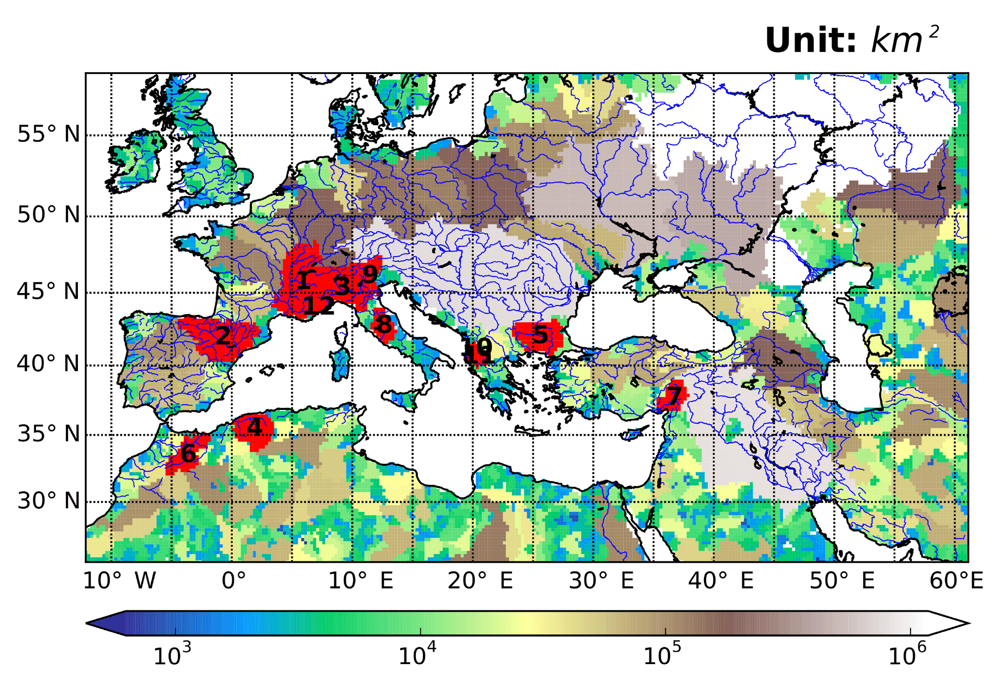
Figure 1Extended simulation domain. The main watersheds are colourized as a function of maximum upstream area (km2). They were extracted for an ORCHIDEE resolution of 1∕4∘, with a threshold HTU number of 50. The 12 river basins studied are coloured in red. The river network is plotted in blue based on the data set from the Generic Mapping Tools (http://gmt.soest.hawaii.edu, last access: 3 December 2018). The river names are Rhône, Ebro, Po, Chelif, Maritsa, Moulouya, Ceyhan, Tiber, Adige, Shkumbinit, Devollit, and Var corresponding to the numbers from 1 to 12, respectively.
Table 1Information on stations used for validation.
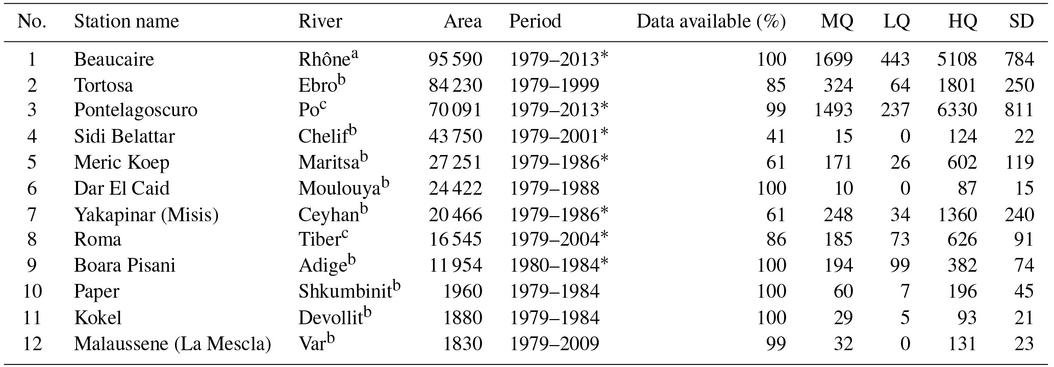
* Daily data are available. Area: catchment area upstream of gauging station (km2); MQ: monthly mean discharge (m3 s−1); LQ: minimum value of monthly discharge (m3 s−1); HQ: maximum value of monthly discharge (m3 s−1); and SD: standard deviation of monthly discharge series (m3 s−1). Observation data are sourced from La Banque Hydro, the GRDC, or Luca Brocca (CNR-IRPI), respectively.
2.2 Numerical design
The RRS is integrated into the ORCHIDEE land surface model (Krinner et al., 2005), where the surface water budget and the resulting surface and subsurface run-off fluxes are estimated by a multi-layer soil hydrology scheme (De Rosnay et al., 2002). In this study, the model is forced by atmospheric forcing data, and three data sets are available, all based on the WATCH Forcing ERA-Interim data set (Weedon et al., 2014). They differ by the precipitation data set they are combined with to obtain bias-corrected precipitation: (1) the CRU data set (Harris et al., 2014); (2) the GPCCv5 data set (Schneider et al., 2014); and (3) the MSWEP data set (Beck et al., 2017). The first two forcing data sets are at a 1∕2∘ spatial resolution, and the latter is at 1∕4∘ resolution. The simulation period extends from 1979 to 2013 after a 10-year spin-up. The time step of ORCHIDEE is 30 min, whilst the time step of the RRS is 1 h, which is compatible with the abovementioned spatial resolutions based on previous theoretical experiments (not shown).
3.1 General framework
The original routing scheme in the ORCHIDEE LSM implements the linear reservoir routing method with river network building on a 1∕2∘ global map of the main watersheds (Oki et al., 1999; Vörösmarty et al., 2000). A brief description of this scheme can be found in Ngo-Duc et al. (2007a) and Guimberteau et al. (2012a). Each river basin is constructed by connecting a number of sub-basins which are defined inside the ORCHIDEE grid boxes, following eight outflow directions. In other words, each sub-basin represents the section of the river basin within the grid box. A sub-basin can be smaller than the ORCHIDEE grid box if the ORCHIDEE model runs at a coarser resolution than 1∕2∘ and each grid box might encompass sub-basins of different rivers. Hereafter, we will use the term “hydrological transfer unit” (HTU) to designate these sub-grid basins. Run-off from one grid box can flow into a neighbouring one or stay in the same grid box, depending on the downstream HTUs. Thus, we propose to call our scheme a “unit-to-unit routing” to distinguish it from the classical grid-to-grid routing.
To describe the transformation of run-off into river discharge along the river network, each particular HTU consists of three linear reservoirs with decreasing water residence times; these reservoirs describe the lags imposed onto groundwater flow, overland flow, and streamflow (Hagemann and Dümenil, 1997; Miller et al., 1994). The lag times are the product of a slope index (k), characterizing the HTU, and a constant specific to the type of reservoir (g), calibrated by Ngo-Duc et al. (2007a). The values of g are 0.24, 3, and 25 (day km−1) for the stream, overland, and groundwater reservoirs, respectively. Following Ducharne et al. (2003), the slope index is given by , where d and S are the respective distance and slope between a pixel and its downstream pixel. It is first defined at the 1∕2∘ resolution and then averaged across all 1∕2∘ pixels composing a HTU. Surface run-off and drainage, which are computed by the soil moisture module of the ORCHIDEE model, are first lagged locally by the overland and groundwater reservoirs, then they are routed along the river network through a linear cascade of stream reservoirs. Applications of this scheme not only enhance the study of large-scale water balance (Ngo-Duc et al., 2005a, c), but they also allow for the simulation of various interactions between rivers and their watersheds (De Rosnay et al., 2003; Guimberteau et al., 2012a, b).
The availability of a high-resolution DEM (digital elevation model), namely HydroSHEDS (Lehner et al., 2008), has presented the opportunity to modify this routing scheme, with the ability to constructing more adequate HTUs in each ORCHIDEE grid box. This new RRS with a higher-resolution river graph can operate at a fine spatial resolution (e.g. finer than 10 km) and is expected to better represent the complexity of river basins and respond better to the inhomogeneity of precipitation patterns. The next sub-section briefly presents the HydroSHEDS data set, and the following sub-sections elaborate on the modifications made to the original routing scheme of ORCHIDEE to create this new version.
3.2 HydroSHEDS data
As a seamless near-global hydrological data set, HydroSHEDS is a suitable database for improving the river routing scheme in the ORCHIDEE model. It is available at resolutions from 3 to 30 arcsec, and provides all of the required information including hydrologically conditioned elevation, drainage directions, and watershed boundaries. Derived from the Shuttle Radar Topography Mission, the quality of HydroSHEDS has the limitations of this radar product, returning a complex mix of terrain elevation and vegetation height, and only covering the land areas from 56∘ S to 60∘ N due to the shuttle's orbit. Despite tremendous effort to void-fill and properly condition the drainage directions some errors remain, such as spurious inland sinks, whilst the assumption of single flow direction prevents river bifurcations, including deltas, from being properly described (Lehner et al., 2008). Nevertheless, this database is widely considered as the best available DEM for hydrological applications, and has shown its advantages for large-scale high-resolution river routing (Gong et al., 2011; Yamazaki et al., 2011). The stream network in HydroSHEDS is comparable with other global hydrographic data such as HYDRO1k, ArcWorld, and the Digital Chart of the World (Lehner et al., 2006).
In this study, we use a resolution of 30 arcsec (1∕120∘ with a pixel size of 0.86 km2 – ca. 1 km at the Equator). It is believed to be sufficient for large-scale applications, and offers the possibility to complete the region north of 60∘ N with the HYDRO1k database at 1 km to achieve full global information (Lehner et al., 2008; Marthews et al., 2015; Wu et al., 2012). A preliminary quality control of HydroSHEDS was performed to ensure that all pixels drain to ocean or to a recognized endorheic basin. This was based on a non-exhaustive comparison with the global ESA-CCI land cover classification (Bontemps et al., 2013) to verify the existence of lakes or wetlands at inland outflow points. This procedure also provided an identifier for all of the river basins with an identified outlet, in particular for the small coastal basins with a zero ID in HydroSHEDS. Based on the elevation, flow directions, and basin/outlet identifier, the following information could be calculated for each HydroSHEDS pixel for further use: slope index, flow accumulation (quantifying the amount of upstream pixels), and total downstream distance to the outlet (ocean or lake).
3.3 HTU and river basin construction
As mentioned above, the major improvement of the new RRS is the possibility to better describe the geometry of the river basins by defining high-resolution HTUs beneath the ORCHIDEE grid-mesh. Figure 2a shows the major steps carried out in the river basin construction. There are two steps that control the number of HTUs in an ORCHIDEE grid-mesh which is an important issue for unit-to-unit routing with respect to the limitation of computational resources. First, the model user needs to specify the maximum area of a HTU in an ORCHIDEE grid cell which allows for the preservation of as much of the hydrological information of HydroSHEDS as required. Second, the user specifies the maximum number of HTUs. If this threshold is exceeded, in the last step of the river network construction, the number of HTUs is reduced by merging smaller units and thus increasing the average HTU's area.
The construction of the HTUs is illustrated in Fig. 2b for the Rhône River (98 000 km2 in Switzerland and south-eastern France, with an outlet in the Mediterranean Sea near Marseille) and an ORCHIDEE grid-mesh resolution of 1∕8∘. For clarity, we impose a maximum number of nine HTUs per ORCHIDEE grid box in this study, but the optimal HTU number is discussed in Sect. 4. In this framework, the number of upstream HTUs contributing water to each ORCHIDEE grid cell is depicted in Fig. 2b. Logically, the ORCHIDEE grid cells which cover the main stream of the Rhône River have a large number of upstream HTUs; therefore the main stream is denoted using dark blue, while smaller tributaries are identified in yellow. This river basin design depends on the arrangement of HTUs inside each ORCHIDEE grid box, as shown by the simple example in Fig. 2c–d. These two figures outline the definition of HTUs in the ORCHIDEE grid cell that is marked by the orange rectangle in Fig. 2b.
All of the outlets from the grid box are identified, and then all of the HydroSHEDS pixels sharing the same grid box outlet are combined to build preliminary HTUs (Fig. 2c). Following this step, a preliminary HTU can be larger than the aforementioned user-defined size (e.g. a user can set the maximum area of a HTU to 2 % of the ORCHIDEE grid box). For instance, the largest preliminary HTU in Fig. 2c covers about 80 % of the grid box area. Hence, a procedure was developed to partition these large preliminary HTUs to the user-defined size. The partitioning process relies on the Pfafstetter topological coding system for streams and basins (Verdin and Verdin, 1999): the flow accumulation is used to identify the main stream of the HTU to partition, and its four main tributaries; this results in the division of the large HTU into nine smaller HTUs which comprises the basins of the four tributaries and five inter-HTUs. All of the coloured HTUs in Fig. 2d initially belong to the preliminary HTU flowing out of the grid box at the outlet point marked by the orange circle on the eastern edge. The division process will continue if the HTU size is larger than the user-defined size, which can obviously not be smaller than the HydroSHEDS pixels (ca. 0.86 km2).
While the delineation based on the Pfafstetter codification informs on the connectivity between the HTUs deriving from the same preliminary HTU (inside one ORCHIDEE grid box), the linkage between HTUs belonging to different grid boxes requires a supplementary procedure. After a HTU is constructed it gets a unique identifier, and the corresponding HTU outlet is located (as the pixel with the biggest flow accumulation). We further calculate the total area upstream from the HTU outlet, and the distance from the HTU outlet to the river basin outlet (ocean or endorheic lake). A complex procedure uses this information to identify the downstream HTU in neighbouring grid boxes, and re-establish the connectivity and coherence of the river network. The advantage of this procedure is the possibility to function on both regular and non-regular grids. Finally, the last step not only ensures the final number of HTUs does not exceed the user-defined threshold (e.g. nine HTUs per grid box in the case of Fig. 2b) but also balances the HTU areas to avoid excessive asymmetry of the HTUs' area distribution. This is done by combining the smallest HTUs that flow out of the ORCHIDEE grid box. Note that the number of tiny HTUs increases remarkably as the ORCHIDEE resolution decreases (e.g. coarser than 1∕4∘). For example, there are tiny preliminary HTUs which only include one HydroSHEDS pixel, as marked by the orange squares in Fig. 2d.
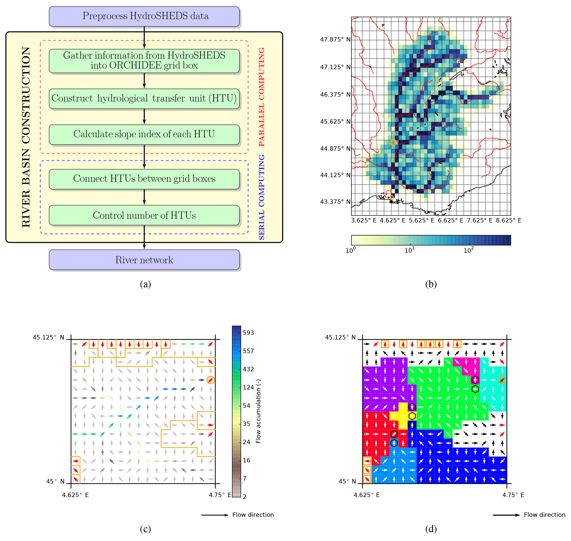
Figure 2A schematic diagram of catchment construction in the new river routing scheme of the ORCHIDEE land surface model (a), and an illustration of the hydrological transfer unit (HTU) idea (b–d). (b) The number of upstream HTUs contributing water to each grid box for the Rhône River at a resolution of 1∕8∘ with a maximum number of nine HTUs per grid box (note the logarithm scale for the coloured legend). Red rivers come from the Generic Mapping Tools data set (http://gmt.soest.hawaii.edu, last access: 3 December 2018). The small orange box shows the grid box displayed in (c) and (d). (c) The orange ORCHIDEE grid box in (b) with information derived from HydroSHEDS at a 30 arcsec resolution: arrows show the flow direction of each HydroSHEDS pixel, the coloured legend shows flow accumulation, bold red arrows show the flow direction of the grid box outlets, the orange lines delineate the boundary of the preliminary HTUs, and the orange circle highlights the outlet points of the largest preliminary HTU in this grid box. (d) Partitioning of HTUs that share the same grid box outlet (marked by the orange circle). Hexagons denote the outlets of inter-HTUs based on the Pfafstetter codification, and the coloured shading indicates the different HTUs. Flow direction arrows are displayed in black and white. Orange squares highlight the approximate 1 km2 HTUs.
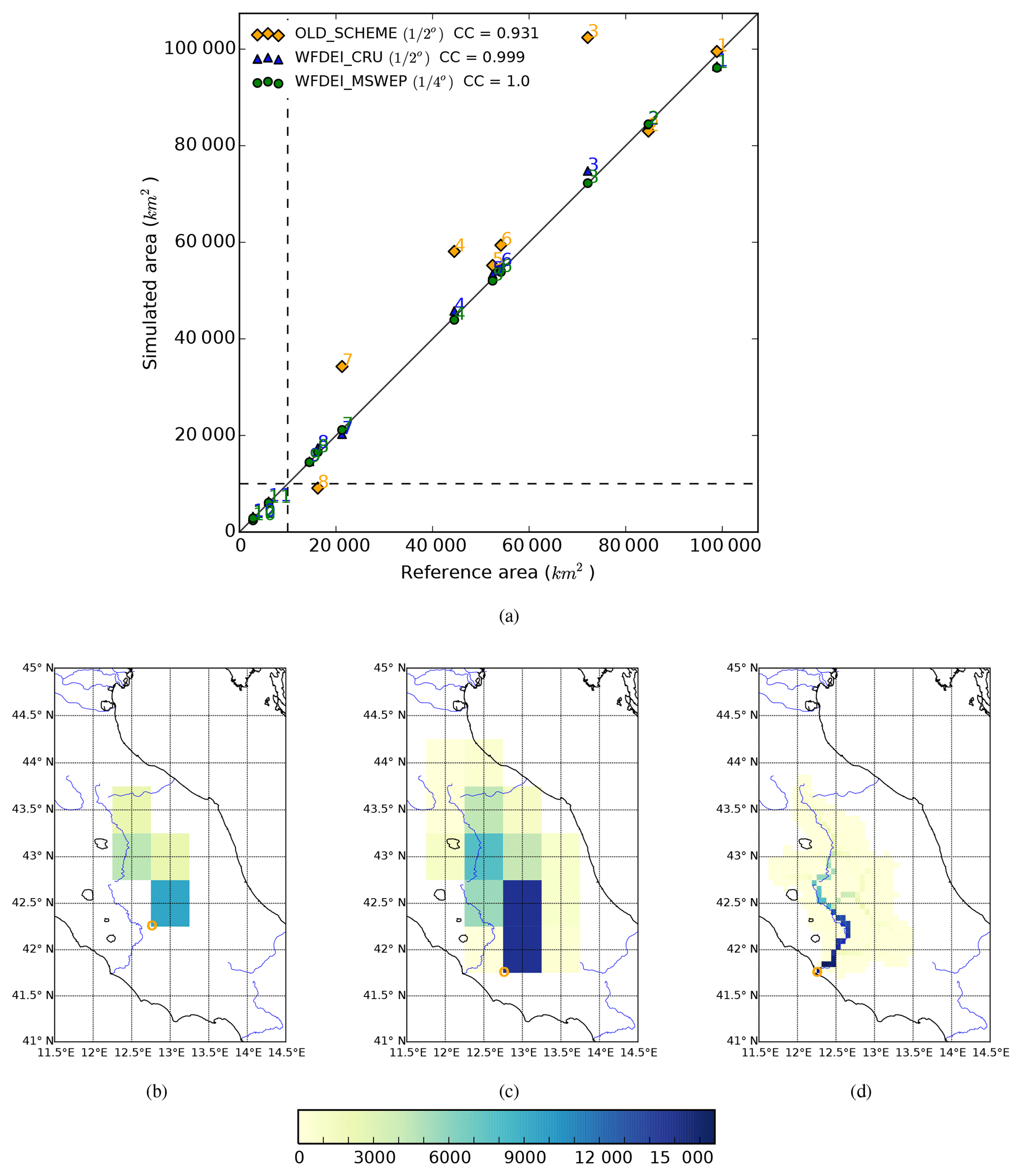
Figure 3Comparison of the modelled area (using the old and new RRS) and the reference area (from Wu et al., 2012) for the 12 river basins in this study (a). Representation of the Tiber River basin in the ORCHIDEE model with the old (b) and new (c) RRS at a regular latitude–longitude grid of 1∕2∘, and with the new RRS at a grid of 1∕16∘ (c). In (b–d), the colours denote the upstream area (km2) contributing water to each grid box, the orange circle is the outlet point, and blue rivers come from the Generic Mapping Tools data set (http://gmt.soest.hawaii.edu).
3.4 Limitation of the old RRS
The river basin construction described above is the solution for the main limitation of the old RRS – its poor representation of small river catchments, i.e. catchments with an area under 2500 km2 (). The reason for this shortfall is that the old RRS implements the river network with a basin description at a 1∕2∘ resolution (Oki et al., 1999; Vörösmarty et al., 2000). Figure 3a compares the simulated areas of 12 river basins in this study to a reference area, which is from the global river network data at 1∕16∘ spatial resolution (Wu et al., 2012). The blue triangles and green circles denote the modelled area in the new RRS with the ORCHIDEE resolutions of 1∕2 and 1∕4∘, respectively. The modelled areas in the old RRS with the 1∕2∘ resolution are shown by the orange diamonds. The numbers correspond to the river names given in Table 1. Significantly, the new RRS accurately constructs the river basin area of all 12 rivers (i.e. the CC values are 0.99 and 1.0). The old RRS only represents the area of the Rhône (1), the Ebro (2) and the Maritsa River (5) well, while the errors are high for other rivers such as the Po (3), the Chelif (4), and the Ceyhan River (7). In addition, the old RRS can not represent four small river basins (i.e. the Adige (9), the Shkumbinit (10), the Devollit (11), and the Var rivers (12)). Figure 3b shows the description of the Tiber River basin (in Italy, with an outlet to the Tyrrhenian Sea at Roma station) with the old RRS and a regular latitude–longitude grid at a resolution of 1∕2∘. This river basin covers only four grid boxes with a maximum upstream area of about 9100 km2, whereas the upstream area of the Roma station is about 16 545 km2 according to the GRDC database. In this case, the old RRS misses the southern part of the Tiber River basin. The simulated outlet point (shown by orange circle) of the Tiber River is located about 70 km from the coastline. At the same resolution (1∕2∘) the new RRS more satisfactorily depicts the southern part of the Tiber River (Fig. 3c). The total area is about 13 600 km2 with the outlet positioned about 30 km from the coast. As the ORCHIDEE resolution increases, the representation of small rivers become more realistic using the new RRS. An example is shown on a regular latitude–longitude grid at 1∕16∘ in Fig. 3d. The total area of the Tiber River reaches nearly 16 600 km2 and the river mouth is properly placed at the coast. The position of the mouth can vary between one resolution and another because of the changing land-sea mask in ORCHIDEE. Due to the limitation of the old RRS with respect to small catchments (Fig. 3), a comparison of the simulation quality between the old and new RRS is difficult in this region. Therefore, the following sections only focus on understanding the new RRS.
3.5 Water routing process
Surface and subsurface run-off from an ORCHIDEE grid box are distributed to the overland and groundwater reservoir of the embedded HTUs in a fashion proportional to their areas. As in the original routing scheme, run-off is routed downstream with a delay time that is controlled by the number of HTUs along the stream and the properties of each HTU, namely their slope index (k) and reservoir parameter (g); the product of these two metrics defines the time lag of each HTU. The slope index is first calculated at a 1 km resolution based on the slope and length of the HydroSHEDS pixels (i.e. the aforementioned formula in Sect. 3.1), and it needs to be properly aggregated at the HTU scale. When used with the new topographic information based on HydroSHEDS, the simple averaging performed in the original version of the routing scheme leads to the consideration of water travelling a distance of 1 km, which is underestimated for most HTU sizes. We developed a new algorithm that uses the drainage directions and the resulting distance of each pixel from the HTU outlet. In practice, for each pixel, we define K as the sum of all of the 1 km values of k along the corresponding downstream line. The upscaled value of k for the HTU is then given by the product of the sum of K across all the pixels composing the HTU and the fractional area of the HTU. As a result, the slope index of the HTUs changes with the area and length of the stream lines in the HTUs (D), so that the streamflow velocity (given by ) does not depend, or only weakly depends, on the HTU scale. In addition, the three reservoir parameters (g) are recalibrated, leading to values of 0.01, 0.5, and 7.0 (day km−1) for the stream, fast, and slow groundwater reservoirs, respectively, i.e. smaller than with the former 1∕2∘ topographic data. These values were estimated empirically for the Rhône River basin and were implemented over the entire simulated domain. As the objective of our study is to explore the value of the new information brought by the high-resolution watershed descriptions, the parameters were determined so that, on a 1∕2∘ grid and using the finest HTU decomposition, the routing scheme reproduces the quality of the inter-annual variability and annual cycle of the coarse resolution version. This provides a baseline against which the impact of the degradation of the HTU resolution can be evaluated on various grids.
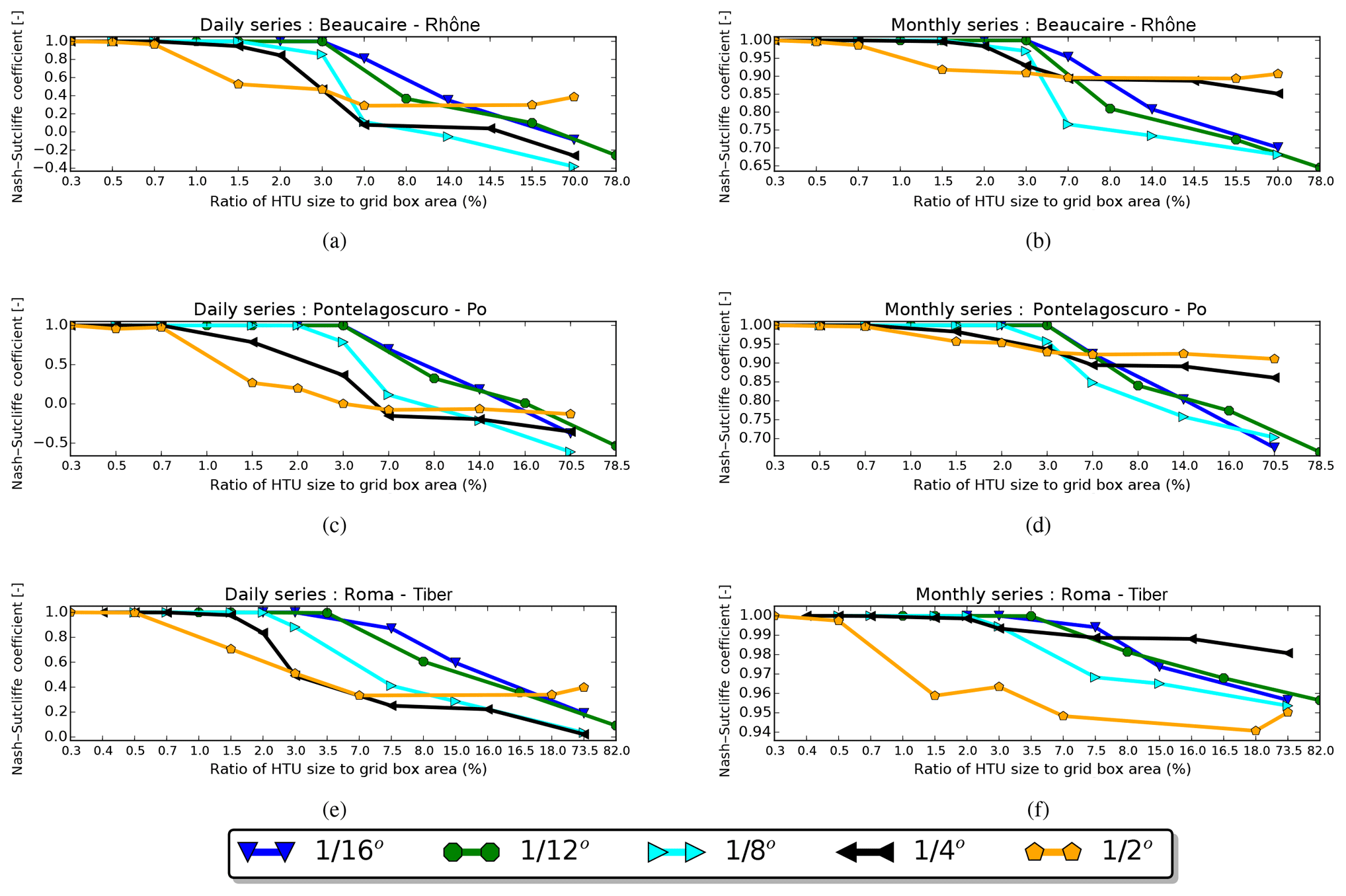
Figure 4Sensitivity of simulation results (Nash–Sutcliffe coefficients) to different HTU sizes (HTU) in the ORCHIDEE mesh, with spatial resolutions varying from 1∕16 to 1∕2∘. The Nash–Sutcliffe coefficient is calculated with respect to the reference case (see the text for details) at daily (a, c, e) and monthly (b, d, f) timescales. Note that the range of the Nash–Sutcliffe coefficient is different for each panel. The x axis gives the ratio of the average HTU size to the ORCHIDEE grid box area (in %). Panels (a) and (b) are Beaucaire station (the Rhône River), (c) and (d) are Pontelagoscuro station (the Po River), and (e) and (f) are Roma station (the Tiber River).
4.1 Experiment design
As previously mentioned, the number of HTUs in each ORCHIDEE grid box increases the computing requirements, but it is also expected to increase the simulation quality, owing to a better description of the river flow directions and basin boundaries. Therefore, here we investigate the impact of the average size of HTUs on the simulated hydrographs, in order to better understand the numerical aspects of the new RRS, and find the best compromise between computational needs and simulation quality. To this end, the ORCHIDEE model is first used without the RRS to generate surface and subsurface run-off at a 1∕4∘ spatial resolution, using the WFDEI_MSWEP atmospheric forcing from 1979 to 2013 (Sect. 2). These fields are then interpolated to four other horizontal resolutions of approximately 1∕16, 1∕12, 1∕8, and 1∕2∘, using the first-order conservative remapping module of the Climate Data Operators (Schulzweida, 2018). These five sets of run-off data are then used to simulate river discharge with the new RRS. For each resolution, a reference case is chosen to preserve most of HydroSHEDS information. This would ideally be achieved with an average HTU size of 0.86 km2, but we used higher values at the coarsest resolutions (1∕4 and 1∕2∘) to limit the computing requirements. As a result, the average HTU areas of the reference cases are approximately 0.86, 0.86, 0.97, 2.60, and 8.20 km2 for resolutions of 1∕16, 1∕12, 1∕8, 1∕4, and 1∕2∘, respectively. These reference HTU areas vary between 2.0 % and 0.3 % of the grid box areas. Finally, for each resolution, several alternative RRS simulations are performed by varying the average HTU size from 0.3 % to about 80 % of the ORCHIDEE grid box areas.
4.2 Results
The analysis of these experiments focuses on three stations: Beaucaire (on the Rhône River, with an upstream area of 95 590 km2), Pontelagoscuro (on the Po River, with an upstream area of 70 091 km2), and Roma (on the Tiber River, with an upstream area of 16 545 km2).
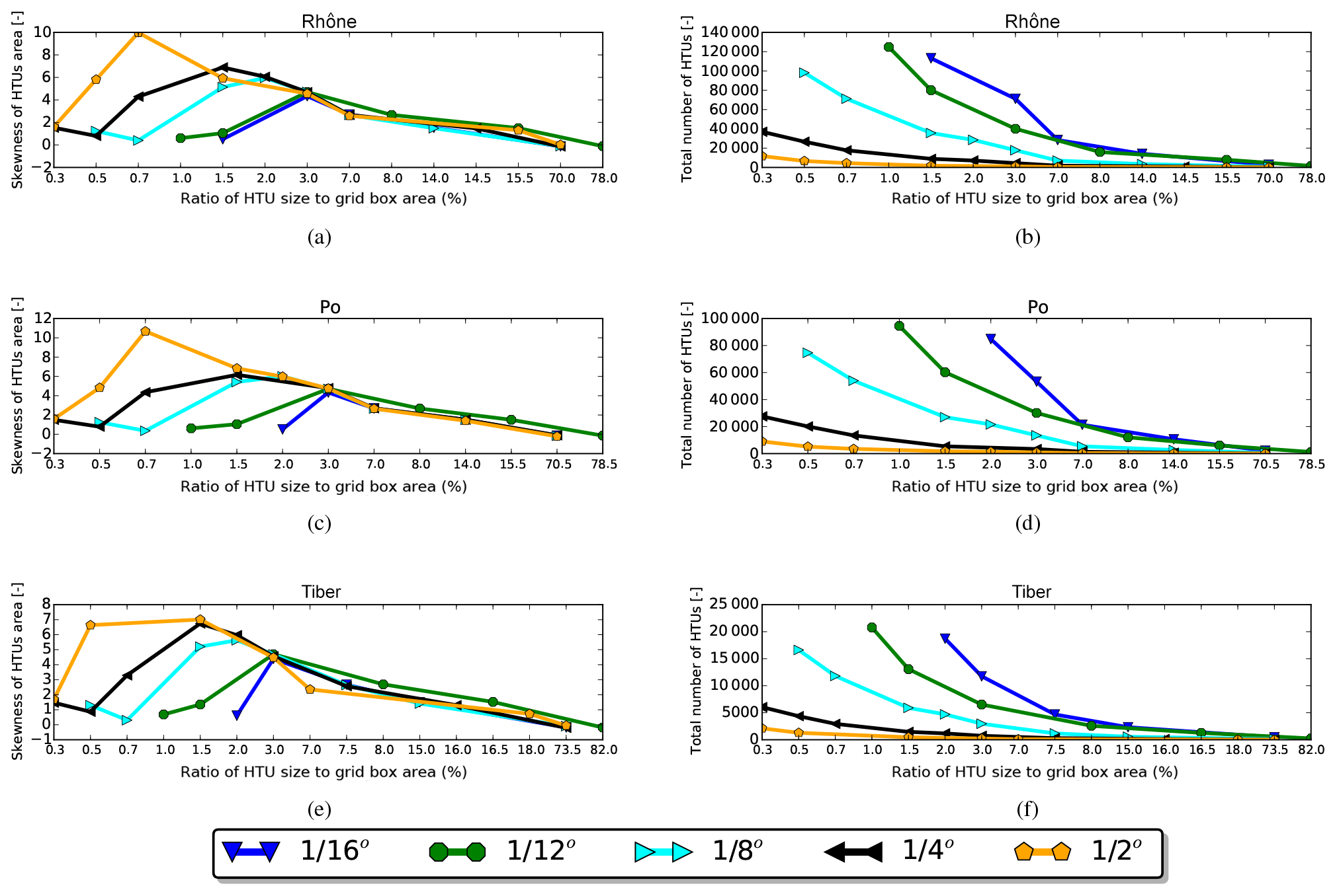
Figure 5Same sensitivity analysis as in Fig. 4, but for the skewness of the HTUs' area distribution (a, c, e) and the total number of HTUs (b, d, f).
Figure 4 shows that, for each resolution, the simulation results degrade when the ratio of the average HTU size to the area of the ORCHIDEE grid box (further abbreviated as the area-ratio) exceeds a certain value. The 1∕2∘ simulations start to deviate remarkably from the reference case when the area-ratio exceeds 0.7 %. For resolutions of 1∕4, 1∕8, 1∕12, and 1∕16∘, the downgrade points are at area-ratios of 1.5 %, 2.0 %, 3.0 %, and 3.0 %, respectively. Another remarkable point is that the degradation is weaker at the monthly than at the daily timescale. At the monthly timescale, the Nash–Sutcliffe coefficient with respect to the reference simulation remains above 0.7, while it drops to a negative value or near zero at the daily timescale. This highlights that the simulation results are more sensitive to the resolution and variation of the HTUs' arrangement at the daily timescale. Nevertheless, the degradation occurs at the same area-ratio for both timescales.
These area-ratio thresholds can be explained by analysing the distribution of HTUs' areas for each resolution (i.e. revealed by the skewness in Fig. 5a, c, e). For all three rivers (the Rhône, the Po, and the Tiber), the skewness peaks at these area-ratio thresholds. Skewness indicates a lack of symmetry produced by the existence of a few much larger HTUs among plenty of smaller ones. The large HTUs appear due to the combination procedure involved to control the number of HTUs. As we move to larger area-ratios, the large and more equal HTUs start to dominate, reducing the skewness of the distribution, and degrading the simulated flow due to a lack of detail in the river graphs and basin characteristics at small area-ratios.
Figure 5b, d, f shows a decrease of the total number of HTUs as the average size ratio of the HTUs increases. The number of HTUs in the case of the 1∕16∘ resolution shows the steepest decrease. For the Rhône River, it decreases from around 120 000 to 3000 HTUs. For a small river such as the Tiber, it also drops from about 18 000 to 500. In contrast, the decreased range for the case of the 1∕2∘ resolution is only about 11 000 and 2000 HTUs for the Rhône River and the Tiber River, respectively. The change of total catchment area and the HTUs' slope factor are also investigated, but their impacts on the behaviour of the new RRS are small (not shown). The simulated basin area only varies strongly in the case of the 1∕2∘ resolution grid. The catchment construction with a resolution higher than 1∕4∘ gives more steady river areas. The examination with other metrics (i.e. correlation coefficient, root mean square error, standard deviation, and kurtosis of the HTU size distribution) supports the following analysis with similar signals, thus it is not shown here.
Figure 6 highlights another aspect of the impact of HTUs' size on the simulated river discharge, by focusing on the performance of the simulations against observed discharge. With the average HTU size maintained at approximately 13 km2 (corresponding to an area-ratio ranging from 0.5 % at 1∕2∘ to 30 % at 1∕16∘), this figure compares monthly simulated river discharge series with the observation data as the ORCHIDEE resolution increases. Therefore, this figure provides a simple investigation on the dependency of the new RRS on the ORCHIDEE resolution. The comparison is focused on two metrics, the Pearson correlation coefficient (CC) and the Nash–Sutcliffe coefficient (NS), calculated at a monthly timescale. These metrics indicate satisfactory performance, with good stability at most resolutions. The only decrease in performance is found at Beaucaire at a 1∕2∘ resolution. As the run-off fluxes were interpolated from the 1∕4∘ to other resolutions, this test does not include the impact of the resolution change on the other components of ORCHIDEE (water and energy budgets). If the full ORCHIDEE model was run at these resolutions, we would expect the changes in run-off and drainage to be larger than the impact of the resolution on the routing demonstrated here. The main point is the stable performance of the RRS at a fixed HTU size (i.e. 13 km2) as the ORCHIDEE resolution varies. Although the new RRS inherently depends on the ORCHIDEE resolution as it implements a unit-to-unit routing method, it can be seen that with a certain average HTU size a stable simulation quality can be expected for a wide range of ORCHIDEE resolutions.
4.3 Practical HTU size
At a given resolution of the ORCHIDEE model, a higher area-ratio (ratio of average HTU size to the ORCHIDEE grid box area) means less HTUs and thus less computational requirements. Conversely, the abovementioned analysis regarding the numerical behaviour of the new RRS indicates that the quality of the simulations deteriorates at large area-ratios, and that this degradation starts at the area-ratio corresponding to the highest skewness of the HTU size distribution. Thus, it can be assumed that the best compromise between simulation quality and computational cost is achieved at this practical HTU size, which seems rather constant across the basins studied. Here, for the 1∕2∘ resolution, we find a practical area-ratio of 0.7 %, corresponding to a practical average HTU size of about 22 km2; for the 1∕4∘ resolution, the practical area-ratio is 1.5 %, corresponding to a practical average HTU size of about 11 km2. This allows a strong computational gain compared to RRS simulations that would be carried out at the highest possible resolution (ca. 0.86 km2), and a gain by a factor of 10 is obtained for the recommended resolution. For the domain discussed here at a resolution of 1∕2∘ and a 33-year simulation period, the ORCHIDEE model without routing takes 5 h (wall-clock time) on a 64 core computational node of the IPSL MesoCentre (https://mesocentre.ipsl.fr/, last access: 3 December 2018). At full HTU resolution the routing adds 30 h to this simulation, while in the optimized configuration the simulation only adds 3 h. Thus, the high-resolution routing with a practical area-ratio of 0.7 % only increases computing time for ORCHIDEE by 60 %.
Table 2Evaluation metrics for monthly river discharge simulations by the ORCHIDEE model with the new RRS. NS: Nash–Sutcliffe efficiency; PCBIAS: percent bias; and RSR: ratio of root mean square error with observation standard deviation.

(1), (2), and (3) are simulation results with forcing data from WFDEI_CRU, WFDEI_GPCC, and WFDEI_MSWEP, respectively.
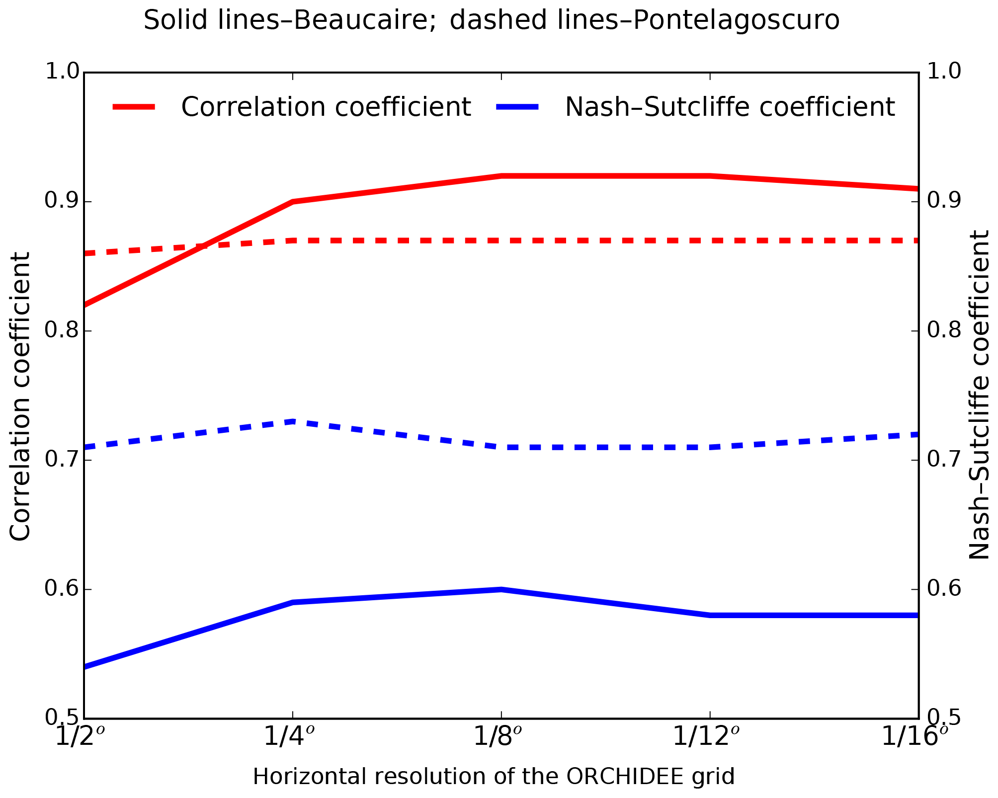
Figure 6Performance of the new RRS as the resolution of the ORCHIDEE mesh changes from 1∕2 to 1∕16∘. All simulations are performed with the same average HTU area of about 13 km2. RRS performance is assessed at a monthly timescale against observed monthly time series at Beaucaire (solid lines) and Pontelagoscuro (dashed lines) stations. Red lines denote the correlation coefficient and blue lines represent the Nash–Sutcliffe coefficient.
5.1 Experiment design
The goal of this section is to evaluate the performance of full ORCHIDEE simulations against river discharge observations. To this end, the new RRS is fully coupled to the ORCHIDEE LSM, which is driven by the three atmospheric forcing data sets presented in Sect. 2: the WFDEI_CRU and WFDEI_GPCC with a spatial resolution of 1∕2∘ and the WFDEI_MSWEP with a spatial resolution of 1∕4∘. The three corresponding simulations are performed with the practical average HTU sizes identified above, viz. 22 km2 at 1∕2∘ and 11 km2 at 1∕4∘. For comparison, similar simulations are also performed with different average HTU sizes (from 0.3 % to 50 % of the grid box area), and also with the old RRS. In the latter case, the ORCHIDEE simulations are only run with the two 1∕2∘ forcing data sets, owing to the limitations of the OLD RRS at finer resolutions. All the simulations extend from 1979 to 2013 after a 10-year spin-up.
5.2 Monthly timescale
Figure 7 shows that the new RRS satisfactorily captures the seasonal cycle of observed discharge at the Beaucaire (the Rhône river) and Pontelagoscuro (the Po river) stations. For Pontelagoscuro, the simulations adequately reproduce two characteristic peaks of the pluvio-nival regime, in October and May. For Beaucaire, the new RRS not only captures the high peak in January but also reproduces the gradual decrease to low flow in August, except with the WFDEI_CRU data. Most simulations also display a positive bias, which can be attributed to excessive run-off fluxes (as the RRS is conservative and does not change the long-term mean discharge) and explained by systematic errors in the water budget parameterization of ORCHIDEE or biases in the three forcing data sets. The purple box plots present the sensitivity of simulated discharge to the average HTU size (from about 0.3 % to about 50 % of the grid box area) and quantify the uncertainty coming from the numerical choices of the scheme. As the HTUs average size varies, the simulated discharge fluctuates in a range which is much smaller (about 40 % smaller) than the magnitude of the bias when compared to observation. In other words, it can be said that the numerical uncertainty is small compared to the uncertainty in the forcing data. According to Beck et al. (2017), the quality of the precipitation data from MSWEP is generally better than WFDEI_CRU when compared with observations from 125 FLUXNET stations. This is confirmed by the lower magnitude of the bias in the case which uses WFDEI_MSWEP (Fig. 7e, f), while this error, when using WFDEI_CRU, is larger at both stations (Fig. 7a, b). Thus, we can confirm that accurate atmospheric forcing is an important factor which determines the performance of a RRS, as already reported by many studies (Guimberteau et al., 2012a; Ngo-Duc et al., 2005c; Pappenberger et al., 2010). In addition, the simulation results using the old RRS (shown by the orange lines in Fig. 7) confirm that the new RRS better matches the observed discharge, which is likely related to its better estimation of the river basin area and structure.

Figure 7Mean annual cycle of river discharge at the Beaucaire (a, c, e) and Pontelagoscuro (b, d, f) stations simulated with three different forcing data sets (WFDEI_CRU: a, b, WFDEI_GPCC: c, d, and WFDEI_MSWEP: e, f). The solid black line shows the observed discharge, and the orange line shows the simulation results with the old RRS. The other lines show simulation results with the new RRS and the practical average HTU size (see text for detail). The small coloured ticks along the y axis give the average values, and the purple box plots show the range of results from simulations with the new RRS and different average HTU sizes (the limits of the boxes correspond to the first and third quartiles).
Validation at the 12 stations highlights that the new RRS simulates acceptable river discharge at a monthly timescale (Fig. 8 and Table 2). The black star shown in the Taylor diagram (Fig. 8) indicates where simulated results would have the same amount of variation and perfect linear correlation with observations. For this reason, simulations that agree well with the observations will lie close to this reference point. Over the 12 stations, the CC are all above 0.6 and the NSDs are in a range from 0.5 to 1.5. The new RRS achieves the best performance at the Beaucaire (1), Pontelagoscuro (3), Yakapinar Misis (7), Kokel (11), Paper (10), Malaussene (12), and Tortosa (2) stations. It is interesting that these stations display a wide range of upstream areas, with a monthly mean discharge from about 30 to 1500 m3 s−1 (Table 1). The worst overall results are found at the Boara Pisani (9), Dar El Caid (6), Roma (8), Sidi Belattar (4), and Meric Koep (5) stations. For Boara Pisani (Adige River, northern Italy), the NSD values from the WFDEI_CRU and WFDEI_MSWEP experiments are both higher than 2.2, which is linked to the high positive bias with these forcing data sets (i.e. the estimated discharge is about twice as high as observations, as shown in Table 2). As the overestimation in the WFDEI_GPCC experiment is smaller (i.e. the PCBIAS is about 22 %), the NSD value stays around 1.10. However, it should be noted that the CC values for this station range from 0.77 to 0.94, so the monthly variability is quite well captured. In particular, the simulated monthly series reproduce the observed hydrological regime well with rather weak seasonal variations and two moderate peaks (in June and October); poor performance is generally found in the driest part of the Mediterranean Basin. The negative bias at Roma station can be attributed to the underestimated run-off during summertime (July to September) or water management practices. The underestimation of discharge is even worse at Sidi Belattar station, which belongs to the longest river in Algeria and rises from the Saharan Atlas. The observed annual mean discharge in this area is lower than 20 m3 s−1, with very low values in summertime (close to zero); none of the simulations can reproduce this characteristic, regardless of the forcing data set utilized. The time series of the anomaly of monthly discharge (with respect to the mean seasonal cycle) are also analysed in Fig. 8b to assess the inter-annual variability of discharge. It shows about the same perspective as the monthly series with lower CC values, although good CC (about 0.9) are still found at Beaucaire (1), Pontelagoscuro (3), and Yakapinar Misis (7) stations. The errors at the Boara Pisani (9), Sidi Belattar (4), and Dar El Caid (6) stations are more clearly demonstrated. Regarding the effect of different forcing data, no clear hierarchy is found, although the above findings confirm that the biases of surface and subsurface run-off by the ORCHIDEE LSM, which are at least partly due to the biases of the forcing data sets, have a strong impact on the simulated streamflow. This is probably the main reason for the low NS values and the high absolute PCBIAS values (shown in Table 2).
Table 3Evaluation metrics for daily river discharge simulations by the ORCHIDEE model using the new RRS: CC – Pearson correlation coefficient; NS – Nash–Sutcliffe efficiency; NSD – normalized standard deviation; CLT – cross-correlation lag time; and RSR – ratio of root mean square error with observation standard deviation.
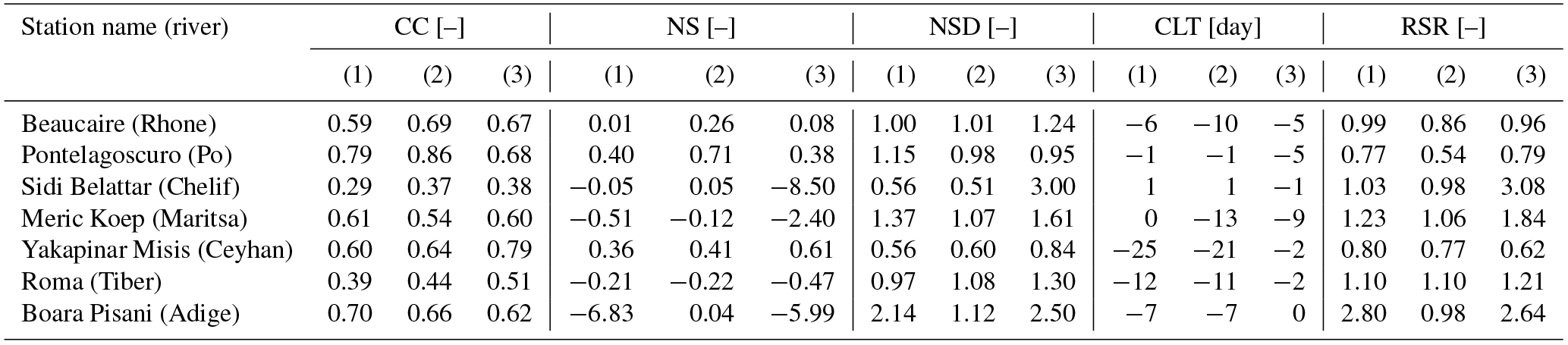
(1), (2), and (3) are simulation results with forcing data from WFDEI_CRU, WFDEI_GPCC, and WFDEI_MSWEP, respectively.
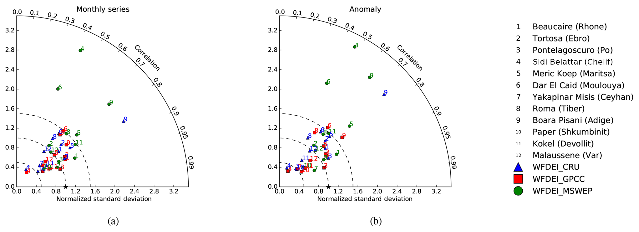
Figure 8Taylor diagrams comparing simulated and observed river discharge at the 12 stations for (a) monthly series and (b) monthly anomalies with respect to the mean seasonal cycle. Blue triangles, red squares, and green circles correspond to simulations with forcing data from WFDEI_CRU, WFDEI_GPCC, and WFDEI_MSWEP, respectively. The number of each station is given in the figure legend and in Table 1. The black star shows the observed value at which the normalized standard deviation and correlation coefficient are 1.0.
It is worthy to note that the impact of human regulation on natural streamflow is neglected in the current version of the new RRS. As a result, irrigation is not represented at all in these simulations, although it is known to play an important role in the Mediterranean region (Margat and Treyer, 2004). According to Montanari (2012), the annual water withdrawal for irrigation in the Po River basin is about 17 km3, i.e. a third of the mean annual discharge (47 km3). Not all withdrawals are transformed into evaporation; thus, a part of these abstractions will return to the river. Nevertheless, one can assume that the observations for Pontelagoscuro (displayed in Fig. 7) probably underestimate the natural river discharge. Snoussi et al. (2002) also underline that the water discharge from the Moulouya River (Dar El Caid station) has been reduced by almost 50 % due to the construction of the Mohamed-V reservoir (in 1967), which could explain the large positive biases of our simulations. Figure 9a shows that, in the Ebro Basin (Spain), the discharge peaks in May and June are largely overestimated by the simulations, regardless of the forcing data set used. However, this is not the case when referring to the observed record from 1920 to 1930. During this period, human impacts on the natural Ebro river flow were not significant and the discharge peak from May to June was stronger than the peak associated with the winter rains. This analysis strongly supports the fact that the overestimation of river discharge over the last decades could be alleviated by a proper representation of human water abstractions for irrigation in the new RRS. For the Maritsa River, Artinyan et al. (2007) noted that about 7 % of the river flow is used for irrigation during summertime (June to August). Despite the fact that this study only covers the year 1996, their findings nevertheless underline the role of anthropogenic influence on river processes, which probably contribute to the positive bias of our simulations. However, in contrast to the Ebro, the spread in the river discharge bias caused by the forcing data uncertainty is larger than the bias itself, suggesting that the role of human processes is not as large in the Maritsa River as it is for the Spanish basin.
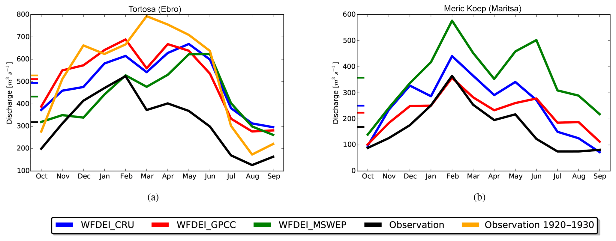
Figure 9Mean annual cycle of river discharge at the Tortosa station on the Ebro River (a) and Meric Koep station on the Maritsa river (b) simulated with forcing data from WFDEI_CRU (blue), WFDEI_GPCC (red), and WFDEI_MSWEP (green). The solid black line is the observation data after 1979, while the orange line is the observation data for the period from 1920 to 1930 (at the Tortosa station). The small coloured ticks along the y axis give the average values.
5.3 Daily timescale
Simulation quality at a daily timescale is validated at seven stations, listed in Table 1. Table 3 presents five metrics considering the variability of daily time series (i.e. CC, NS, NSD, and CLT) and the magnitude of the error (i.e. RSR). The daily CC values are slightly smaller than the monthly CC values, but remain higher than 0.6 for five stations, where the short-term variability of streamflow is correctly reproduced. The best result can be found for the Pontelagoscuro station with forcing data from WFDEI_GPCC (Table 3). The two exceptions are Roma station (Tiber) and Sidi Belattar station (Chelif), which displayed weak CC at the monthly timescale. Table 3 also presents CLT values in a range from −25 days to 1 day, which suggests that some CC values can be improved by accelerating the transfer of water in the RSS. We also find that the daily NS values are much weaker than the monthly values. At the daily timescale, acceptable NS values, which are usually taken as higher than 0.5 (Moriasi et al., 2007; Tavakoly et al., 2017), are only found at the Pontelagoscuro (Po) and Yakapinar Misis (Ceyhan) stations, which are the stations maximizing the monthly NS. The reason for this is that the NS is very sensitive to mass balance errors, i.e. river discharge bias (Gupta and Kling, 2011; Krause et al., 2005), and to daily time series of small dry rivers (Schaefli and Gupta, 2007). Although the NS is very commonly used to evaluate hydrological simulations, this criteria still raises many questions regarding its application (Criss and Winston, 2008; Gupta et al., 2009). The largest biases also explain why all RSR values in Table 3 are larger than 0.5. The large fluctuations of all the metrics between the simulations using the three different forcings again highlight the importance of the accuracy of the atmospheric conditions imposed on the LSM.
For the four stations with the best daily NS values, Fig. 10 visualizes the simulation results at the daily time scale using flow duration curves, which represent the percentage of time over which discharge exceeds the discharge value indicated on the vertical axis. This analysis shows that discharge at Beaucaire station (Fig. 10a) is overestimated over the full range of frequencies, except with WFDEI_MSWEP, which induces lower flows than observed for the 20 % lowest flows (exceedance frequency above 80 %). Except when using WFDEI_CRU forcing data, realistic statistics are found at almost all frequencies at Pontelagoscuro station (Fig. 10b), explaining the good results presented in Table 3. In contrast, at Yakapinar Misis station (Fig. 10c) the RRS captures the low flows under 500 m3 s−1 well, but the highest flows which occur less than 10 % of time are strongly underestimated. The poor performance at the Sidi Belattar station is confirmed by Fig. 10d. At this station, streamflow exceeding 100 m3 s−1 only occurs 5 % of time, whilst more than 50 % of the time the flow is close to zero. It is difficult to capture the daily discharge at this station, and the large agricultural water demand over the Chelif Basin (Mahe et al., 2013) probably contributes to the errors. However, the main error source seems to be the forcing data sets, as the observations fall in their wide uncertainty range.
Streamflow fluctuations possess alternative frequencies in addition to the daily and monthly oscillation. This can be seen in the power spectrum of daily river discharge at Beaucaire in Fig. 11a. The power spectrum corresponds to the squared amplitude at each frequency and was extracted using discrete Fourier transform spectroscopy and was smoothed with a Savitzky–Golay filter (Savitzky and Golay, 1964). It is a robust method for analysing the multi-scale temporal variations in the various variables contributing to the river discharge. As has been shown by Weedon et al. (2015), it facilitates the diagnosis and development of hydrological models. In the power-spectra trend lines for high frequencies (variation faster than 30 days) and low frequencies (slower than 30 days) are also plotted.
Based on the previous diagnostics in Sect. 5.2 and 5.3 we expect the new RRS to replicate the variation of river flow at various frequencies well. Figure 11a shows the good match of the two power spectrum patterns. The β values for the simulation are 0.91 and 2.39 at frequencies above and below 30 days, respectively, very close to the corresponding slopes for the observations, i.e. 0.81 and 2.28. At high frequency, there is a mismatch of the power density around the 3-day period. It can be traced back to the simulated subsurface run-off, which shows a similar peak during the same period (Fig. 11b). The peak at 3 days is probably characteristic of the soil moisture diffusion scheme of the ORCHIDEE model, as it does not have a signature in precipitation and evaporation averaged over the entire Rhône catchment (Fig. 11). The spectra of these two fluxes which characterize the exchange with the atmosphere are more noisy at the synoptic scales (below 15 days) and display a stronger slope for low periods. These results are indicative of soil moisture diffusion in ORCHIDEE that is too fast or of an insufficient buffering of the resulting subsurface flow (drainage) by the routing reservoir representing groundwater flow. It also further suggests that the link between the soil hydrology and the routing scheme is too simple in ORCHIDEE and lacks an appropriate representation of the aquifers. Human activities and the regulation of river flows also affect the river discharge variability at many frequencies (e.g. hydropeaking as a result of the storage for hydropower plants; Meile et al., 2011); thus, the validation of this variability either requires the analysis of pristine catchments or the representation of water management infrastructures in the model.
Nowadays, global hydrology is considered to be an essential component of LSMs and Earth system models (Bierkens, 2015). Recent developments in river routing modelling have allowed for the investigation of the impact of hydrological processes (e.g. floodplains; d'Orgeval et al., 2008) and groundwater interactions (Vergnes et al., 2014) on the climate system, and conversely, the impacts of human regulation and climate change on natural streamflow (Voisin et al., 2013a, b). A strong emphasis has also been placed on high-resolution routing schemes (Ducharne et al., 2003; Yamazaki et al., 2011; Zhao et al., 2017). In this context, the present study allows us to take advantage of the high-resolution HydroSHEDS data in the original RRS of the ORCHIDEE LSM. Figure 1 shows (for the Mediterranean area) that not only is the Danube delineated, with a catchment of about 800 000 km2, but the nearly 2000 km2 Var River basin is also represented. Andersson et al. (2015) denoted that accurate river basin area is the first factor for properly simulating river discharge. Arora et al. (2001) also remarked on the difficulty of reliably simulating river flow for small basins at large spatial scale. The proposed scheme provides a good river network quality over a variety of resolutions and simulation scales, which reduces the need for a network-response function to reduce this scale dependency (Gong et al., 2009). In addition, Verdin and Verdin (1999) highlighted the value of the Pfafstetter codification to preserve river network topology and topographic control of drainage. It supplies a spatial framework which reconciles information from scale of general circulation models (GCMs) to smaller scale river processes (e.g. irrigation operation). Therefore, it provides adaptability to higher resolution input data (e.g. the 3 arcsec HydroSHEDS data) and the control of computing resource as the resolution of atmospheric forcing data changes. We believe that we have designed an innovative infrastructure which will be the basis for further studies regarding the links between the global water cycle and anthropogenic impacts (human regulation as well as climate change) or hydrological processes.
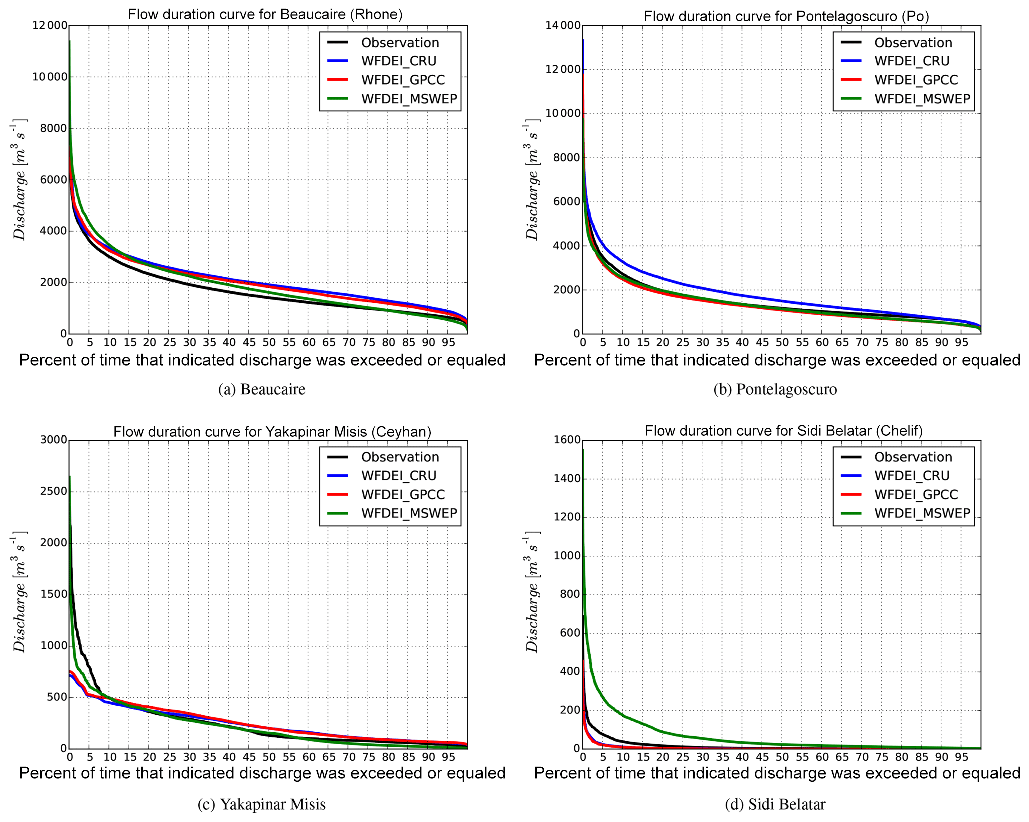
Figure 10Flow duration curve for daily river discharge at the Beaucaire (a), Pontelagoscuro (b), Yakapinar Misis (c), and Sidi Belattar (d) stations. The solid black line is the observation data. The blue, red, and green lines are simulations with forcing data from WFDEI_CRU, WFDEI_GPCC, and WFDEI_MSWEP, respectively.
A number of hydrological processes are still neglected in the current version of the new RRS. Thus, after having demonstrated the numerical robustness of the RRS, we will have the possibility to improve the scheme by adding these missing processes. It is recommended that water management through reservoirs and abstraction should be integrated in the new RRS. The deficit of river discharge in summertime for irrigation is not captured in the new RRS. In addition, hydraulic processes such as water storage in floodplains and swamps should be represented. In fact, the modelling infrastructure of irrigation is integrated in the old RRS of the ORCHIDEE model which is validated over the Indian Peninsula (De Rosnay et al., 2003) and applied to study the impact of irrigation on the onset of the Indian summer monsoon (Guimberteau et al., 2012b). The representation of floodplains and swamps is also included in this old RRS in order to study the surface infiltration processes in the west African hydrological cycle (d'Orgeval et al., 2008) or evaluate the ability of the ORCHIDEE model to simulate streamflow over the Amazon River basin (Guimberteau et al., 2012a). Their importance in a global river routing model is underlined in Ducharne et al. (2003), Yamazaki et al. (2011), and Guimberteau et al. (2012a). Since these representations of human processes or flood plains are based on the hypothesis that HTU are rather large (i.e. at a scale of 1∕2∘), they can be improved to benefit from the high-resolution description of river basins and streams. For instance, the most up-to-date global map of irrigated areas is provided at a 5 arcmin (ca. 10 km) resolution by Siebert et al. (2015). The new RRS describes the river network by connecting HTUs which can vary in size from about 1 km2 to the area of the ORCHIDEE grid cell (e.g. 1∕2∘), meaning that it can account for most heterogeneities of the 5 arcmin map of irrigated areas.
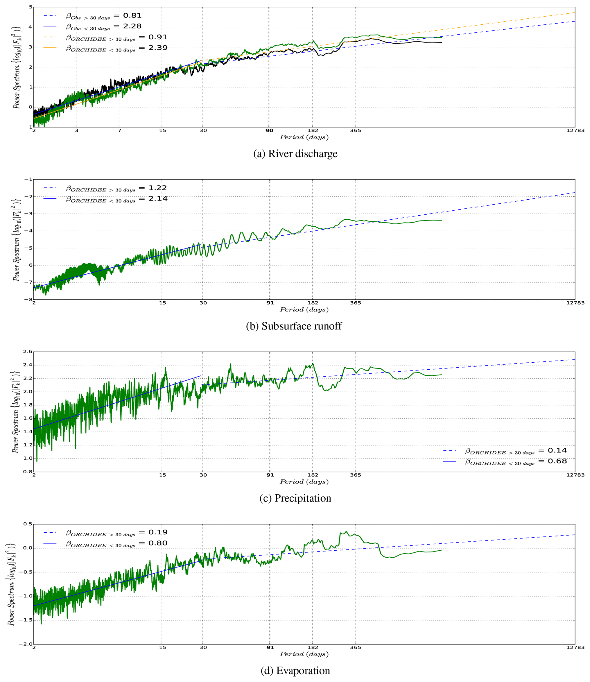
Figure 11Power spectral density of daily river discharge (a) estimated by the ORCHIDEE model at the Beaucaire station (Rhône), and subsurface run-off (b), precipitation (c), and evaporation (d) over the entire Rhône River catchment estimated by ORCHIDEE. The Savitzky–Golay filter with a window of 21 is applied for smoothing the noise signal. The black line is the observation data (Obs) and the green is the ORCHIDEE model results with forcing data from WFDEI_MSWEP (ORCHIDEE). Trend lines for frequency above/below 30 days are shown with their β slope.
Another interesting development path concerns the interactions between the groundwater system and the rivers. Pappenberger et al. (2010) highlights that the groundwater delay parameter is the most sensitive calibration parameter in routing schemes, and a more physically based description of this parameter is being examined for the ORCHIDEE RRS (Schneider, 2017). The RRS also lacks a special treatment for lakes, which could be included based on the ideas of Milly et al. (2014). In the current version, water which flows to lakes is evaporated through the soil moisture module of the ORCHIDEE model. Nevertheless, as the effect of all uncertainty sources (e.g. epistemic uncertainty) is difficult to separately evaluate, the spatial resolution might be an appropriate starting point for investigation. Spacial resolution is not only important for describing human influences, but also for physically describing river flow, although it can lead the present reservoir parameterization to perform poorly. Furthermore, it is worth noting that the evaluation is carried out over 12 small to medium size rivers with different climatic and watershed characteristics. Previous studies have tended to focus on very large rivers or one specific medium-sized catchment (Gong et al., 2009). This limits the generic application of their RRS at the global scale and may require parameter recalibration for smaller-scale implementation. The role of calibration for realistically simulating run-off is discussed in Ducharne et al. (2003) and Beck et al. (2016). However, at this stage of our study, the good representation of complex basin maps provides a satisfactory basis for simulations. The new RRS, which explicitly accounts for the higher quality topographical information from HydroSHEDS, is expected to compensate for the disadvantage of using simple reservoir parameters for all rivers, which is a legacy of the old RRS.
The results presented in this study also show that the new RSS has the potential to adequately reproduce streamflow at daily timescales, which is not an easy task in LSMs. Balsamo et al. (2011) showed preliminary river discharge predictions at daily timescales using the ECMWF land surface scheme. Only a moderate correlation of 0.33 over 211 selected basins was found which is lower than the values presented here; therefore, the new RRS presented in this study provides a powerful tool for good representation of river basins in the ORCHIDEE LSM. Reproducing river run-off at a daily frequency in a global hydrology model often requires the parameterization of complicated processes (Beck et al., 2016; Yamazaki et al., 2011). Further improvements could be expected by describing how stream velocity increases with streamflow, which is important for simulating fluctuations in river discharge at short timescales (Arora and Boer, 1999; Ngo-Duc et al., 2007b). In order to calculate the flow velocity, the river width could be classically obtained using geomorphological relationships with annual mean river discharge (Leopold and Maddock, 1953), although it is also directly available based on remote sensing (Allen and Pavelsky, 2015; Yamazaki et al., 2014). Above all, this study focuses on small river basins in complex topography such as those flowing into the Mediterranean Basin, and there is a need to verify these results at the global scale and on larger basins.
This study presents an attempt to improve the river routing scheme in the ORCHIDEE LSM, in order to benefit from the accurate hydrography provided by the HydroSHEDS database at a 1 km resolution. This high-resolution information is aggregated in hydrological transfer units which are constructed inside each ORCHIDEE grid box. The key advantage of this new scheme is its ability to provide a precise river catchment description over a wide range of scales and more precisely describe the water delay in the various sections of the river basin. River networks which are depicted by connecting these HTUs provide precise flow pathways. The results show a wide range of river catchment sizes can be precisely delineated using the new RRS, which provides improved length and slope information for rivers. This information is improved by the accurate altitude provided by the HydroSHEDS data. This is an important step toward improving the morphological description of river systems, which is known to be a strong constraint on river flow. The new RRS can preserve (as far as possible) the hydrographic details of the 1 km HydroSHEDS data inside each grid box of the ORCHIDEE LSM. It also more precisely locates the river mouth at the coast which will be an asset when coupling the ORCHIDEE LSM into a global or regional Earth system model. In addition, the new RRS can operate on unstructured grids with a resolution of up to 1 km2. This flexibility is clearly an advantage for this RRS compared with other large-scale hydrological models (Kauffeldt et al., 2016).
The new RRS is shown to satisfactorily reproduce the seasonal variations of streamflow in a large range of catchments. In addition to satisfactory simulations at monthly timescale, the new RRS promises the ability to satisfactorily capture higher frequencies in the surface freshwater flows – in particular at daily timescales. In addition, the impact of uncertainty in the forcing data on the simulated discharge is again emphasized. This is consistent with previous studies highlighting the necessity of accurate precipitation inputs for calculating water balance (Decharme and Douville, 2006b; Fekete et al., 2004). For the Mediterranean region we could also note that when the deviations from observations where larger than the forcing uncertainty, human management of water played an important role in the basin. This suggests that anthropogenic processes are probably more critical in this region than our limits on representing geophysical processes. Eventually, this RRS and its planned improvements will enhance Earth system models by producing a more realistic riverine freshwater flux into the Mediterranean Sea and improving the coupling between land and ocean processes.
The source code is freely available online at the following address: http://dx.doi.org/10.14768/06337394-73A9-407C-9997-0E380DAC5593. Readers interested in running the model should follow the instructions at http://orchidee.ipsl.fr/index.php/you-orchidee (last access: 3 December 2018), and contact the corresponding author for a username and password.
TNQ and JP performed the source code modification. AD provided the valuable slope index calculation idea. TNQ and JP designed the experiments, and TNQ carried them out. TNQ, JP and AD prepared the paper with contributions from all coauthors. AS provided the netCDF format of the HydroSHEDS data.
The authors declare that they have no conflict of interest.
The authors acknowledge thoughtful reviews from Lieke Melsen and
Naoki Mizukami. We thank Luca Brocca (CNR-IRPI, Italy) for providing us with
the daily discharge data for Pontelagoscuro and Roma stations. We also
gratefully acknowledge the GRDC (Global Runoff Data Centre) for providing
valuable data. This work was supported by the computing resources of the IPSL
ClimServ cluster at École Polytechnique, France.
Edited by: Chiel van Heerwaarden
Reviewed by:
Lieke Melsen and Naoki Mizukami
Akhil, V., Durand, F., Lengaigne, M., Vialard, J., Keerthi, M., Gopalakrishna, V., Deltel, C., Papa, F., and de Boyer Montégut, C.: A modeling study of the processes of surface salinity seasonal cycle in the Bay of Bengal, J. Geophys. Res.-Oceans, 119, 3926–3947, 2014. a
Allen, G. H. and Pavelsky, T. M.: Patterns of river width and surface area revealed by the satellite-derived North American River Width data set, Geophys. Res. Lett., 42, 395–402, 2015. a, b
Andersson, J., Pechlivanidis, I., Gustafsson, D., Donnelly, C., and Arheimer, B.: Key factors for improving large-scale hydrological model performance, European Water, 49, 77–88, 2015. a
Arora, V., Seglenieks, F., Kouwen, N., and Soulis, E.: Scaling aspects of river flow routing, Hydrol. Process., 15, 461–477, 2001. a
Arora, V. K. and Boer, G. J.: A variable velocity flow routing algorithm for GCMs, J. Geophys. Res.-Atmos., 104, 30965–30979, 1999. a
Arora, V. K., Chiew, F. H., and Grayson, R. B.: A river flow routing scheme for general circulation models, J. Geophys. Res., 104, 314–347, 1999. a
Artinyan, E., Habets, F., Noilhan, J., Ledoux, E., Dimitrov, D., Martin, E., and Le Moigne, P.: Modelling the water budget and the riverflows of the Maritsa basin in Bulgaria, Hydrol. Earth Syst. Sci., 12, 21–37, https://doi.org/10.5194/hess-12-21-2008, 2008. a
Balsamo, G., Beljaars, A., Scipal, K., Viterbo, P., van den Hurk, B., Hirschi, M., and Betts, A. K.: A revised hydrology for the ECMWF model: Verification from field site to terrestrial water storage and impact in the Integrated Forecast System, J. Hydrometeorol., 10, 623–643, 2009. a
Balsamo, G., Pappenberger, F., Dutra, E., Viterbo, P., and Van den Hurk, B.: A revised land hydrology in the ECMWF model: a step towards daily water flux prediction in a fully-closed water cycle, Hydrol. Process., 25, 1046–1054, 2011. a, b, c
Beck, H. E., van Dijk, A. I. J. M., de Roo, A., Dutra, E., Fink, G., Orth, R., and Schellekens, J.: Global evaluation of runoff from 10 state-of-the-art hydrological models, Hydrol. Earth Syst. Sci., 21, 2881–2903, https://doi.org/10.5194/hess-21-2881-2017, 2017. a, b, c
Beck, H. E., van Dijk, A. I. J. M., Levizzani, V., Schellekens, J., Miralles, D. G., Martens, B., and de Roo, A.: MSWEP: 3-hourly 0.25∘ global gridded precipitation (1979–2015) by merging gauge, satellite, and reanalysis data, Hydrol. Earth Syst. Sci., 21, 589–615, https://doi.org/10.5194/hess-21-589-2017, 2017. a, b
Beven, K. J. and Cloke, H. L.: Comment on “Hyperresolution global land surface modeling: Meeting a grand challenge for monitoring Earth's terrestrial water” by Eric F. Wood et al., Water Resour. Res., 48, W01801, https://doi.org/10.1029/2011WR010982, 2012. a
Bierkens, M. F.: Global hydrology 2015: State, trends, and directions, Water Resour. Res., 51, 4923–4947, 2015. a
Bierkens, M. F., Bell, V. A., Burek, P., Chaney, N., Condon, L. E., David, C. H., Roo, A., Döll, P., Drost, N., Famiglietti, J. S., Flörke, M., Gochis D. J., Houser, P., Hut, R., Keune, J., Kollet, S., Maxwell, R., Reager, J. T., Samaniego, L., Sudicky, E., Sutanudjaja, E. H., Giesen, N., Winsemius, H., and Wood, E. F.: Hyper-resolution global hydrological modelling: what is next?, Hydrol. Process., 29, 310–320, 2015. a
Bontemps, S., Defourny, P., Radoux, J., Van Bogaert, E., Lamarche, C., Achard, F., Mayaux, P., Boettcher, M., Brockmann, C., Kirches, G., Zülkhe, M., Kalogirou, V., Seifert, F. M., and Arino, O.: Consistent global land cover maps for climate modelling communities: current achievements of the ESA's land cover CCI, in: Proceedings of the ESA Living Planet Symposium, Edimburgh, 9–13, 2013. a
Criss, R. E. and Winston, W. E.: Do Nash values have value? Discussion and alternate proposals, Hydrol. Process., 22, 2723–2725 https://doi.org/10.1002/hyp.7072, 2008. a
David, C. H., Maidment, D. R., Niu, G.-Y., Yang, Z.-L., Habets, F., and Eijkhout, V.: River network routing on the NHDPlus dataset, J. Hydrometeorol., 12, 913–934, 2011. a
Decharme, B. and Douville, H.: Introduction of a sub-grid hydrology in the ISBA land surface model, Clim. Dynam., 26, 65–78, 2006a. a
Decharme, B. and Douville, H.: Uncertainties in the GSWP-2 precipitation forcing and their impacts on regional and global hydrological simulations, Clim. Dynam., 27, 695–713, 2006b. a
De Rosnay, P., Polcher, J., Bruen, M., and Laval, K.: Impact of a physically based soil water flow and soil-plant interaction representation for modeling large-scale land surface processes, J. Geophys. Res.-Atmos., 107, 4118, https://doi.org/10.1029/2001JD000634, 2002. a
De Rosnay, P., Polcher, J., Laval, K., and Sabre, M.: Integrated parameterization of irrigation in the land surface model ORCHIDEE. Validation over Indian Peninsula, Geophys. Res. Lett., 30, 1986, https://doi.org/10.1029/2003GL018024, 2003. a, b, c
Döll, P. and Lehner, B.: Validation of a new global 30-min drainage direction map, J. Hydrol., 258, 214–231, 2002. a
d'Orgeval, T., Polcher, J., and de Rosnay, P.: Sensitivity of the West African hydrological cycle in ORCHIDEE to infiltration processes, Hydrol. Earth Syst. Sci., 12, 1387–1401, https://doi.org/10.5194/hess-12-1387-2008, 2008. a, b
Drobinski, P., Ducrocq, V., Alpert, P., Anagnostou, E., Béranger, K., Borga, M., Braud, I., Chanzy, A., Davolio, S., Delrieu, G., Estournel, C., Filali Boubrahmi, N., Font, J., Grubišić, V., Gualdi, S., Homar, V., Ivančan-Picek, B., Kottmeier, C., Kotroni, V., Lagouvardos, K., Lionello, P., Llasat, C., Ludwig, W., Lutoff, C., Mariotti, A., Richard, E., Romero, R., Rotunno, R., Ruin, I., Roussot, O., Somot, S., Taupier-Letage, I., Tintoré, J., Uijlenhoet, R., and Wernli, H.: HyMeX: A 10-year multidisciplinary program on the Mediterranean water cycle, B. Am. Meteorol. Soc., 95, 1063–1082, 2014. a
Dubos, T., Dubey, S., Tort, M., Mittal, R., Meurdesoif, Y., and Hourdin, F.: DYNAMICO-1.0, an icosahedral hydrostatic dynamical core designed for consistency and versatility, Geosci. Model Dev., 8, 3131–3150, https://doi.org/10.5194/gmd-8-3131-2015, 2015. a
Ducharne, A., Golaz, C., Leblois, E., Laval, K., Polcher, J., Ledoux, E., and de Marsily, G.: Development of a high resolution runoff routing model, calibration and application to assess runoff from the LMD GCM, J. Hydrol., 280, 207–228, 2003. a, b, c, d, e, f
Fekete, B. M., Vörösmarty, C. J., Roads, J. O., and Willmott, C. J.: Uncertainties in precipitation and their impacts on runoff estimates, J. Climate, 17, 294–304, 2004. a
Fekete, B. M., Looser, U., Pietroniro, A., and Robarts, R. D.: Rationale for monitoring discharge on the ground, J. Hydrometeorol., 13, 1977–1986, 2012. a
Gong, L., Widen-Nilsson, E., Halldin, S., and Xu, C.-Y.: Large-scale runoff routing with an aggregated network-response function, J. Hydrol., 368, 237–250, 2009. a, b
Gong, L., Halldin, S., and Xu, C.-Y.: Global-scale river routing—an efficient time-delay algorithm based on HydroSHEDS high-resolution hydrography, Hydrol. Process., 25, 1114–1128, 2011. a, b
Guimberteau, M., Drapeau, G., Ronchail, J., Sultan, B., Polcher, J., Martinez, J.-M., Prigent, C., Guyot, J.-L., Cochonneau, G., Espinoza, J. C., Filizola, N., Fraizy, P., Lavado, W., De Oliveira, E., Pombosa, R., Noriega, L., and Vauchel, P.: Discharge simulation in the sub-basins of the Amazon using ORCHIDEE forced by new datasets, Hydrol. Earth Syst. Sci., 16, 911–935, https://doi.org/10.5194/hess-16-911-2012, 2012a. a, b, c, d, e, f
Guimberteau, M., Laval, K., Perrier, A., and Polcher, J.: Global effect of irrigation and its impact on the onset of the Indian summer monsoon, Clim. Dynam., 39, 1329–1348, 2012b. a, b, c
Gupta, H. V. and Kling, H.: On typical range, sensitivity, and normalization of Mean Squared Error and Nash-Sutcliffe Efficiency type metrics, Water Resour. Res., 47, W10601, https://doi.org/10.1029/2011WR010962, 2011. a
Gupta, H. V., Kling, H., Yilmaz, K. K., and Martinez, G. F.: Decomposition of the mean squared error and NSE performance criteria: Implications for improving hydrological modelling, J. Hydrol., 377, 80–91, 2009. a
Hagemann, S. and Dümenil, L.: A parametrization of the lateral waterflow for the global scale, Clim. Dynam., 14, 17–31, 1997. a
Harris, I., Jones, P., Osborn, T., and Lister, D.: Updated high-resolution grids of monthly climatic observations – the CRU TS3.10 Dataset, Int. J. Climatol., 34, 623–642, 2014. a
Jensen, T. G., Wijesekera, H. W., Nyadjro, E. S., Thoppil, P. G., Shriver, J. F., Sandeep, K., and Pant, V.: Modeling salinity exchanges between the equatorial Indian Ocean and the Bay of Bengal, Oceanography, 29, 92–101, 2016. a
Kauffeldt, A., Wetterhall, F., Pappenberger, F., Salamon, P., and Thielen, J.: Technical review of large-scale hydrological models for implementation in operational flood forecasting schemes on continental level, Environ. Modell. Softw., 75, 68–76, 2016. a, b
Koirala, S., Yeh, P. J.-F., Hirabayashi, Y., Kanae, S., and Oki, T.: Global-scale land surface hydrologic modeling with the representation of water table dynamics, J. Geophys. Res.-Atmos., 119, 75–89, 2014. a
Krause, P., Boyle, D. P., and Bäse, F.: Comparison of different efficiency criteria for hydrological model assessment, Adv. Geosci., 5, 89–97, https://doi.org/10.5194/adgeo-5-89-2005, 2005. a
Krinner, G., Viovy, N., de Noblet-Ducoudré, N., Ogée, J., Polcher, J., Friedlingstein, P., Ciais, P., Sitch, S., and Prentice, I. C.: A dynamic global vegetation model for studies of the coupled atmosphere-biosphere system, Global Biogeochem. Cy., 19, GB1015, https://doi.org/10.1029/2003GB002199, 2005. a
Lea, D., Mirouze, I., Martin, M., King, R., Hines, A., Walters, D., and Thurlow, M.: Assessing a new coupled data assimilation system based on the Met Office coupled atmosphere–land–ocean–sea ice model, Mon. Weather Rev., 143, 4678–4694, 2015. a
Lehner, B., Verdin, K., and Jarvis, A.: HydroSHEDS technical documentation, version 1.0, World Wildlife Fund US, Washington, DC, 1–27, 2006. a
Lehner, B., Verdin, K., and Jarvis, A.: New global hydrography derived from spaceborne elevation data, EOS, 89, 93–94, 2008. a, b, c, d
Leopold, L. B. and Maddock, T.: The hydraulic geometry of stream channels and some physiographic implications, Vol. 252, US Government Printing Office, 1953. a
Mahe, G., Lienou, G., Descroix, L., Bamba, F., Paturel, J.-E., Laraque, A., Meddi, M., Habaieb, H., Adeaga, O., Dieulin, C., Chahnez Kotti, F., and Khomsi, K.: The rivers of Africa: witness of climate change and human impact on the environment, Hydrol. Process., 27, 2105–2114, 2013. a
Margat, J. and Treyer, S.: L'eau des Méditerranéens: situation et perspectives. PNUE-PAM, Tech. rep., Plan Bleu, Technical Report Series, 2004. a
Marthews, T. R., Dadson, S. J., Lehner, B., Abele, S., and Gedney, N.: High-resolution global topographic index values for use in large-scale hydrological modelling, Hydrol. Earth Syst. Sci., 19, 91–104, https://doi.org/10.5194/hess-19-91-2015, 2015. a
Meile, T., Boillat, J.-L., and Schleiss, A.: Hydropeaking indicators for characterization of the Upper-Rhone River in Switzerland, Aquat. Sci., 73, 171–182, 2011. a
Miller, J. R., Russell, G. L., and Caliri, G.: Continental-scale river flow in climate models, J. Climate, 7, 914–928, 1994. a
Milly, P. C., Malyshev, S. L., Shevliakova, E., Dunne, K. A., Findell, K. L., Gleeson, T., Liang, Z., Phillipps, P., Stouffer, R. J., and Swenson, S.: An enhanced model of land water and energy for global hydrologic and earth-system studies, J. Hydrometeorol., 15, 1739–1761, 2014. a, b
Montanari, A.: Hydrology of the Po River: looking for changing patterns in river discharge, Hydrol. Earth Syst. Sci., 16, 3739–3747, https://doi.org/10.5194/hess-16-3739-2012, 2012. a
Moriasi, D. N., Arnold, J. G., Van Liew, M. W., Bingner, R. L., Harmel, R. D., and Veith, T. L.: Model evaluation guidelines for systematic quantification of accuracy in watershed simulations, T. ASABE, 50, 885–900, 2007. a, b
Nassopoulos, H., Dumas, P., and Hallegatte, S.: Adaptation to an uncertain climate change: cost benefit analysis and robust decision making for dam dimensioning, Climatic Change, 114, 497–508, 2012. a
Ngo-Duc, T., Laval, K., Polcher, J., and Cazenave, A.: Contribution of continental water to sea level variations during the 1997–1998 El Niño–Southern Oscillation event: Comparison between Atmospheric Model Intercomparison Project simulations and TOPEX/Poseidon satellite data, J. Geophys. Res.-Atmos., 110, D09103, https://doi.org/10.1029/2004JD004940, 2005a. a, b
Ngo-Duc, T., Laval, K., Polcher, J., Lombard, A., and Cazenave, A.: Effects of land water storage on global mean sea level over the past half century, Geophys. Res. Lett., 32, 2005b. a
Ngo-Duc, T., Polcher, J., and Laval, K.: A 53-year forcing data set for land surface models, J. Geophys. Res.-Atmos., 110, D06116, https://doi.org/10.1029/2004JD005434, 2005c. a, b, c
Ngo-Duc, T., Laval, K., Ramillien, G., Polcher, J., and Cazenave, A.: Validation of the land water storage simulated by Organising Carbon and Hydrology in Dynamic Ecosystems (ORCHIDEE) with Gravity Recovery and Climate Experiment (GRACE) data, Water Resour. Res., 43, W04427, https://doi.org/10.1029/2006WR004941, 2007a. a, b, c
Ngo-Duc, T., Oki, T., and Kanae, S.: A variable streamflow velocity method for global river routing model: model description and preliminary results, Hydrol. Earth Syst. Sci. Discuss., 4, 4389–4414, https://doi.org/10.5194/hessd-4-4389-2007, 2007b. a, b, c
Oki, T. and Sud, Y.: Design of Total Runoff Integrating Pathways (TRIP – A global river channel network, Earth Interact., 2, 1–37, 1998. a, b
Oki, T., Nishimura, T., and Dirmeyer, P.: Assessment of annual runoff from land surface models using Total Runoff Integrating Pathways (TRIP), J. Meteorol. Soc. Jpn. Ser. II, 77, 235–255, 1999. a, b, c, d
Oleson, K. W., Lawrence, D. M., Gordon, B., Flanner, M. G., Kluzek, E., Peter, J., Levis, S., Swenson, S. C., Thornton, E., Feddema, J., Heald, C. L., Lamarque, J.-F., Niu, G.-Y., Qian, T., Running, S., Sakaguchi, K., Yang, L., Zeng, X., Zeng, X., and Decker, M.: Technical description of version 4.0 of the Community Land Model (CLM), NCAR Technical Note NCAR/TN-478+STR, 257, 2010. a
Pappenberger, F., Cloke, H., Balsamo, G., Ngo-Duc, T., and Oki, T.: Global runoff routing with the hydrological component of the ECMWF NWP system, Int. J. Climatol., 30, 2155–2174, 2010. a, b, c, d
Polcher, J.: Les processus de surface à l'échelle globale et leurs interactions avec l'atmosphère, Habilitation à diriger des recherches, Université Paris VI, 2003. a
Satoh, M., Tomita, H., Yashiro, H., Miura, H., Kodama, C., Seiki, T., Noda, A. T., Yamada, Y., Goto, D., Sawada, M., Miyoshi, T., Niwa, Y., Hara, M., Ohno, T., Iga, S., Arakawa, T., Inoue, T., and Kubokawa, H.: The Non-hydrostatic Icosahedral Atmospheric Model: description and development, Progress in Earth and Planetary Science, 1, 1–32, 2014. a
Savitzky, A. and Golay, M. J.: Smoothing and differentiation of data by simplified least squares procedures, Anal. Chem., 36, 1627–1639, 1964. a
Schaefli, B. and Gupta, H. V.: Do Nash values have value?, Hydrol. Process., 21, 2075–2080, 2007. a
Schneider, A.: Estimation of the base flow time constant for global scale applications, PhD thesis, Université Pierre et Marie Curie, Paris, France, available at: https://www.metis.upmc.fr/~ducharne/documents/these_SCHNEIDER_2017.pdf (last access: 3 December 2018), 2017. a
Schneider, U., Becker, A., Finger, P., Meyer-Christoffer, A., Ziese, M., and Rudolf, B.: GPCC's new land surface precipitation climatology based on quality-controlled in situ data and its role in quantifying the global water cycle, Theor. Appl. Climatol., 115, 15–40, 2014. a
Schulzweida, U.: Climate Data Operators (CDO) User Guide, Max Planck Institute for Meteorologie, available at: https://code.mpimet.mpg.de/projects/cdo/embedded/cdo.pdf (last access: 3 December 2018), 2018. a
Sevault, F., Somot, S., Alias, A., Dubois, C., Lebeaupin-Brossier, C., Nabat, P., Adloff, F., Déqué, M., and Decharme, B.: A fully coupled Mediterranean regional climate system model: design and evaluation of the ocean component for the 1980–2012 period, Tellus A, 66, https://doi.org/10.3402/TELLUSA.V66.23967, 2014. a
Siebert, S., Kummu, M., Porkka, M., Döll, P., Ramankutty, N., and Scanlon, B. R.: A global data set of the extent of irrigated land from 1900 to 2005, Hydrol. Earth Syst. Sci., 19, 1521–1545, https://doi.org/10.5194/hess-19-1521-2015, 2015. a
Snoussi, M., Haïda, S., and Imassi, S.: Effects of the construction of dams on the water and sediment fluxes of the Moulouya and the Sebou Rivers, Morocco, Reg. Environ. Change, 3, 5–12, 2002. a
Souty, F., Brunelle, T., Dumas, P., Dorin, B., Ciais, P., Crassous, R., Müller, C., and Bondeau, A.: The Nexus Land-Use model version 1.0, an approach articulating biophysical potentials and economic dynamics to model competition for land-use, Geosci. Model Dev., 5, 1297–1322, https://doi.org/10.5194/gmd-5-1297-2012, 2012. a
Tavakoly, A. A., Snow, A. D., David, C. H., Follum, M. L., Maidment, D. R., and Yang, Z.-L.: Continental-Scale River Flow Modeling of the Mississippi River Basin Using High-Resolution NHDPlus Dataset, J. Am. Water Resour. As., 53, 258–279, 2017. a
Turuncoglu, U. U., Giuliani, G., Elguindi, N., and Giorgi, F.: Modelling the Caspian Sea and its catchment area using a coupled regional atmosphere-ocean model (RegCM4-ROMS): model design and preliminary results, Geosci. Model Dev., 6, 283–299, https://doi.org/10.5194/gmd-6-283-2013, 2013. a
Verdin, K. L. and Verdin, J. P.: A topological system for delineation and codification of the Earth's river basins, J. Hydrol., 218, 1–12, 1999. a, b
Vergnes, J.-P., Decharme, B., and Habets, F.: Introduction of groundwater capillary rises using subgrid spatial variability of topography into the ISBA land surface model, J. Geophys. Res.-Atmos., 119, 11065–11086, https://doi.org/10.1002/2014JD021573, 2014. a
Vilibić, I., Mihanović, H., Janeković, I., and Šepić, J.: Modelling the formation of dense water in the northern Adriatic: Sensitivity studies, Ocean Model., 101, 17–29, 2016. a
Voisin, N., Li, H., Ward, D., Huang, M., Wigmosta, M., and Leung, L. R.: On an improved sub-regional water resources management representation for integration into earth system models, Hydrol. Earth Syst. Sci., 17, 3605–3622, https://doi.org/10.5194/hess-17-3605-2013, 2013a. a
Voisin, N., Liu, L., Hejazi, M., Tesfa, T., Li, H., Huang, M., Liu, Y., and Leung, L. R.: One-way coupling of an integrated assessment model and a water resources model: evaluation and implications of future changes over the US Midwest, Hydrol. Earth Syst. Sci., 17, 4555–4575, https://doi.org/10.5194/hess-17-4555-2013, 2013b. a
Von Bloh, W., Rost, S., Gerten, D., and Lucht, W.: Efficient parallelization of a dynamic global vegetation model with river routing, Environ. Modell. Softw., 25, 685–690, 2010. a
Vörösmarty, C., Fekete, B., Meybeck, M., and Lammers, R.: Global system of rivers: Its role in organizing continental land mass and defining land-to-ocean linkages, Global Biogeochem. Cy., 14, 599–621, 2000. a, b, c, d
Walters, D. N., Williams, K. D., Boutle, I. A., Bushell, A. C., Edwards, J. M., Field, P. R., Lock, A. P., Morcrette, C. J., Stratton, R. A., Wilkinson, J. M., Willett, M. R., Bellouin, N., Bodas-Salcedo, A., Brooks, M. E., Copsey, D., Earnshaw, P. D., Hardiman, S. C., Harris, C. M., Levine, R. C., MacLachlan, C., Manners, J. C., Martin, G. M., Milton, S. F., Palmer, M. D., Roberts, M. J., Rodríguez, J. M., Tennant, W. J., and Vidale, P. L.: The Met Office Unified Model Global Atmosphere 4.0 and JULES Global Land 4.0 configurations, Geosci. Model Dev., 7, 361–386, https://doi.org/10.5194/gmd-7-361-2014, 2014. a
Weedon, G. P., Balsamo, G., Bellouin, N., Gomes, S., Best, M. J., and Viterbo, P.: The WFDEI meteorological forcing data set: WATCH Forcing Data methodology applied to ERA-Interim reanalysis data, Water Resour. Res., 50, 7505–7514, 2014. a
Weedon, G. P., Prudhomme, C., Crooks, S., Ellis, R. J., Folwell, S. S., and Best, M. J.: Evaluating the performance of hydrological models via cross-spectral analysis: case study of the Thames Basin, UK, J. Hydrometeorol., 16, 214–231, 2015. a
Wood, E. F., Roundy, J. K., Troy, T. J., Van Beek, L., Bierkens, M. F., Blyth, E., de Roo, A., Döll, P., Ek, M., Famiglietti, J., Gochis, D., van de Giesen, N., Houser, P., Jaffe, P. R., Kollet, S., Lehner, B., Lettenmaier, D. P., PetersLidard, C., Sivapalan, M., Sheffield, J., Wade, A., and Whitehead, P.: Hyperresolution global land surface modeling: Meeting a grand challenge for monitoring Earth's terrestrial water, Water Resour. Res., 47, W05301, https://doi.org/10.1029/2010WR010090, 2011. a
Wu, H., Kimball, J. S., Li, H., Huang, M., Leung, L. R., and Adler, R. F.: A new global river network database for macroscale hydrologic modeling, Water Resour. Res., 48, W09701, https://doi.org/10.1029/2012WR012313, 2012. a, b, c
Yamazaki, D., Kanae, S., Kim, H., and Oki, T.: A physically based description of floodplain inundation dynamics in a global river routing model, Water Resour. Res., 47, W04501, https://doi.org/10.1029/2010WR009726, 2011. a, b, c, d, e
Yamazaki, D., O'Loughlin, F., Trigg, M. A., Miller, Z. F., Pavelsky, T. M., and Bates, P. D.: Development of the Global Width Database for Large Rivers, Water Resour. Res., 50, 3467–3480, https://doi.org/10.1002/2013WR014664, 2014. a
Zhao, F., Veldkamp, T. I. E., Frieler, K., Schewe, J., Ostberg, S., Willner, S., Schauberger, B., Gosling, S. N., Schmied, H. M., Portmann, F. T., Leng, G., Huang, M., Liu, X., Tang, Q., Hanasaki, N., Biemans, H., Gerten, D., Satoh, Y., Pokhrel, Y., Stacke, T., Ciais, P., Chang, J., Ducharne, A., Guimberteau, M., Wada, Y., Kim, H., and Yamazaki, D.: The critical role of the routing scheme in simulating peak river discharge in global hydrological models, Environ. Res. Lett., 12, 075003, https://doi.org/10.1088/1748-9326/aa7250, 2017. a