A continuum model (PSUMEL1) of ice mélange and its role during retreat of the Antarctic Ice Sheet

Pollard, David; DeConto, Robert M.; Alley, Richard B.

doi:https://doi.org/10.5194/gmd-11-5149-2018

Articles | Volume 11, issue 12

https://doi.org/10.5194/gmd-11-5149-2018

Articles | Volume 11, issue 12

Model description paper

20 Dec 2018

Model description paper |

| 20 Dec 2018

A continuum model (PSUMEL1) of ice mélange and its role during retreat of the Antarctic Ice Sheet

David Pollard, Robert M. DeConto, and Richard B. Alley

Abstract

Rapidly retreating thick ice fronts can generate large amounts of mélange (floating ice debris), which may affect episodes of rapid retreat of Antarctic marine ice. In modern Greenland fjords, mélange provides substantial back pressure on calving ice faces, which slows ice front calving rates. On the much larger scales of West Antarctica, it is unknown if mélange could clog seaways and provide enough back pressure to act as a negative feedback slowing retreat. Here we describe a new mélange model, using a continuum-mechanical formulation that is computationally feasible for long-term continental Antarctic applications. It is tested in an idealized rectangular channel and calibrated very basically using observed modern conditions in Jakobshavn fjord, West Greenland. The model is then applied to drastic retreat of Antarctic ice in response to warm mid-Pliocene climate. With mélange parameter values that yield reasonable modern Jakobshavn results, Antarctic marine ice still retreats drastically in the Pliocene simulations, with little slowdown despite the huge amounts of mélange generated. This holds both for the rapid early collapse of West Antarctica and for later retreat into major East Antarctic basins. If parameter values are changed to make the mélange much more resistive to flow, far outside the range for reasonable Jakobshavn results, West Antarctica still collapses and retreat is slowed or prevented only in a few East Antarctic basins.

Download & links

Article (PDF, 8544 KB)

How to cite

How to cite.

Dates

Received: 02 Feb 2018 – Discussion started: 13 Mar 2018 – Revised: 23 Nov 2018 – Accepted: 04 Dec 2018 – Published: 20 Dec 2018

1 Introduction

Theory, modeling and observations point to the prospect of rapid grounding-line retreat and marine ice loss from West Antarctica and major East Antarctic basins, in response to climate warming (Weertman, 1974; Mercer, 1978; Schoof, 2007; Pritchard et al., 2012; Rignot et al., 2014). These rapid retreats are suspected to have contributed to high sea level stands in the Pliocene and Pleistocene (Rovere et al., 2014; Dutton et al., 2015; Pollard et al., 2015; Sutter et al., 2016), and pose the threat of drastic sea level rise due to future warming (Joughin et al., 2014a; Cornford et al., 2015; Feldmann and Levermann, 2015; Golledge et al., 2015; Ritz et al., 2015; DeConto and Pollard, 2016; Arthern and Williams, 2017). The retreats are thought to be amplified by runaway positive-feedback mechanisms, termed marine ice sheet instability (MISI; Schoof, 2007) and/or marine ice cliff instability (MICI; Pollard et al., 2015; DeConto and Pollard, 2016), that occur in marine basins whose bedrock topography deepens into the interior, due to the very strong dependence of ice export on grounding-line depth.

Calving of ice from thick (∼1 km) glacial termini generates substantial amounts of floating ice debris called mélange, as observed in the fjords of major outlet glaciers of Greenland and in places in Antarctica (Macayeal et al., 1998; Joughin et al., 2008, 2014b; Fricker et al., 2009; Khazendar et al., 2009; Amundson et al., 2010; Scambos et al., 2011). In Greenland, mélange occupies some or all of the fjords downstream of the ice terminus (Joughin et al., 2012; Sundal et al., 2013; Sutherland et al., 2014; Moon et al., 2015) and is thought to provide significant back pressure on the ice face, reducing calving and ice velocities especially in winter (Joughin et al., 2008, 2014b; Amundson et al., 2010; Walter et al., 2012; Todd et al., 2014). The lateral scales of these modern ice faces and fjords are 5 to 10 km. If large-scale retreat is initiated in the Amundsen Sea sector of West Antarctica, for instance, the lateral scales of retreating grounding lines would potentially be an order of magnitude larger (hundreds of kilometers), flowing into relatively unconfined seaways, for which there is no modern analog. Vast amounts of mélange would presumably be generated, and it is unknown whether the mélange could act as a significant negative feedback, through clogging of seaways and back pressure on ice faces, reducing calving and slowing ice velocities and grounding-line retreat.

Here we formulate an explicit physically based model of mélange and couple it to an existing ice sheet–shelf model. To date, only a few studies have modeled mélange explicitly, and most use discrete-particle or granular-material approaches for ice and/or mélange (Bassis and Jacobs, 2013; Astrom et al., 2014; Peters et al., 2015; Robel, 2017; Burton et al., 2018). Discrete-particle models are potentially truer representations of real mélange (in Greenland fjords today, a poorly sorted agglomeration of ice pieces with sizes up to O(100 m)) but are computationally infeasible for the temporal and spatial scales involved in Antarctic retreat.

Our approach is to use continuum physics, in a model that captures basic dependencies between rate of mélange supply, downstream export, side drag and ocean bottom resistance, which combine to produce back pressure on ice faces. Two other continuum models have been applied to mélange to our knowledge (Seneca Lindsey and Dupont, 2012; Vankova and Holland, 2017), discussed briefly in Sect. 3.

2 Relationship with Greenland fjords

We calibrate the model using basic observations of modern mélange in the Jakobshavn fjord. (For simplicity we use the term Jakobshavn throughout and do not use separate names for the glacier and fjord, Jakobshavn Isbræ and Ilulissat Icefjord, respectively.) There are no comprehensive datasets of mélange properties in Jakobshavn or other fjords to our knowledge, but there are many individual studies with relevant observations and modeling (Joughin et al., 2008, 2014b; Amundson et al., 2008, 2010; Motyka et al., 2011; MacAyeal et al., 2012; Walter et al., 2012; Cook et al., 2014; Sundal et al., 2013; Foga et al., 2014; Foga, 2016; Sutherland et al., 2014; Todd et al., 2014; Cassotto et al., 2015; Krug et al., 2015; Moon et al., 2015; Murray et al., 2015; Enderlin et al., 2016; Burton et al., 2018). The main properties reported in these studies that are pertinent here, with quantities rounded to the nearest order of magnitude for Jakobshavn, are as follows.

Mélange consists of discrete ice pieces, densely packed or loosely cemented within sea ice, with the mass dominated by ice pieces, the largest of which are small compared to the fjord dimensions, as required for a continuum approach.

Mélange is generated (supplied) by calving from a ∼1 km thick grounded ice front. The ice velocity just upstream of the front is ∼10 km yr⁻¹, and the mélange just downstream of the front is ∼100 m thick. At the ice front, the kilometer-scale calving pieces (icebergs) must overturn and disintegrate very rapidly to maintain an initial mélange thickness of ∼100 m. This occurs primarily in discrete events that episodically push the mélange downstream in rapid pulses. Currents, winds and tides may also move the mélange but are assumed to be minor here. By conservation of mass, the mélange must move away from the ice front at an average speed ∼10 times that of the incoming ice, thinning and/or slowing further down the fjord due to basal or surface melting.

There is a pronounced seasonal cycle. In winter, the mélange is stiffened by the gluing effect of sea ice, enabling side drag to be transmitted as increased back pressure on the ice face, which prevents calving and allows a small floating ice tongue to form; the existing mélange and ice front move down the fjord together at the incoming ice speed (∼10 km yr⁻¹). In summer, the mélange is more deformable, back stress is less, the ice tongue is lost and episodic calving of ∼ km scale icebergs resumes, which pushes the mélange in the bulk of the fjord rapidly downstream in discrete pulses. On an annual mean basis the mélange moves down the fjord at tens of kilometers per year to the mouth in Disko Bay, where it disperses and melts.

For now, we consider the ice and mélange state in only the modern Jakobshavn fjord, leaving past variations (Csatho et al., 2008; Joughin et al., 2008; Young et al., 2011) for possible future work. The model formulated below does not simulate discrete calving events, but rather the long-term average results of many such events. It does not simulate seasonal cycles of freezing–thawing sea ice and shutdown–resumption of calving, but it represents the resulting annual average behavior. In particular there is no seasonal advance and retreat of model grounding lines, just annual mean motion.

At first sight this seems to pose a dilemma in applying the model to Jakobshavn and other Greenland fjords where the seasonal cycle plays a role, with mélange being pushed gradually downstream by the advancing glacier face in winter and new mélange being created by episodic calving in summer that pushes existing mélange rapidly downstream in discrete pulses. The net effect is a horizontal “pump” that pushes the entire mélange body down the whole length of the fjord while the annual mean grounding-line position remains stationary. Despite the absence of a seasonal cycle, our model captures this “push–pump” mechanism via the boundary condition Eq. (B2) on mélange velocity at the ice interface, as described in Appendix B. As described below, mélange can also be driven downstream in the model by local hydrostatic pressure gradients, from thicker mélange at the head to thinner mélange at the mouth. Both the push–pump and pressure gradient mechanisms are active in our Jakobshavn simulations.

The model formulation is described in Sect. 3, including discussion of the continuum-mechanics approach. Idealized channel tests are performed in Sect. 4.1, and the basic calibration vs. Jakobshavn is described in Sect. 4.2. The model is applied to continental Antarctica in Sect. 4.3, with simulations of drastic ice retreat during the warm mid-Pliocene (∼3 Ma). Conclusions on the role of mélange in Antarctic retreat are summarized in Sect. 5.

3 Formulation

One possible choice for a continuum-mechanical model of mélange is the viscous-plastic (VP) fluid formulation developed for sea ice (Hibler, 1977; Hibler and Tucker, 1979), which has been used and extended in many subsequent studies (e.g., Hunke and Dukowicz, 1997) including a simplified cavitating-fluid (CF) version (Flato and Hibler, 1992). Recently Vankova and Holland (2017) used cavitating-fluid dynamics in a continuum model of mélange. Their model is quite different from ours, explicitly incorporating large icebergs within a matrix of sea ice, and may be suited for smaller scales than considered here. For the continental and millennial scales of Antarctic ice retreat, the following considerations guided our choice of continuum model.

The VP-CF approach involves the concept of an internal pressure that resists convergence, which is an empirical function of sea ice thickness and represents ridging of ice slabs. As noted by Vankova and Holland (2017), ridging is not relevant for mélange, but this function can still be used to represent resistance to convergence when large ice pieces in the mélange become closely packed. Instead of using a VP-CF approach, we use shallow-shelf approximation (SSA) equations commonly used for ice shelf dynamics, modified to include (i) strong resistance to convergence beyond a certain “packing density” and (ii) very little resistance to divergence. With these modifications, the resulting system functions quite similarly to a CF model, but we feel it has some advantages, including adjustable nonlinear rheology and inclusion of hydrostatic pressure gradients, as described below.

In this preliminary study, for simplicity we use only one variable to represent mélange amount, h_m. It is called “thickness” below but can be interpreted as a combination of thickness and density of the ice pieces responsible for most of the stresses in the mélange. A second prognostic variable could be added to represent compactness or fractional cover as in sea ice models (A in Hibler, 1977; Flato and Hibler, 1992), but given the uncertainties in mélange rheology we choose to start with just one variable, h_m. Strong resistance to convergence beyond a certain packing density is included as a pressure term P_p in the equations below, which is zero for small h_m and ramps up strongly as h_m exceeds a certain value.

If mélange never overrode itself so as to increase its bulk thickness, P_p would be the only pressure term needed. This appears to be the case for the largest bergs embedded in Greenland mélange (O(100)m; Enderlin et al., 2016), for which compressive forces are never strong enough to cause overriding. However, overriding is conceivable for smaller pieces and may be more common on the much larger scales of Antarctica. This process is represented in the equations below simply by using the vertically integrated hydrostatic pressure gradient within the mélange.

New mélange is supplied by calving or cliff failure of a solid ice face, added to the adjacent grid cell. This either is pushed downstream by the moving ice face (see Appendix B) or piles up locally, increasing the local pressure and the velocities away from the face, so that a balance between supply and downstream advection is reached.

Following the considerations discussed above, we utilize and adapt the SSA-scaled equations, used in many studies to describe ice shelf and ice stream flow with very little basal drag, in which nearly all of the flow is due to horizontal stretching and vertical shear is negligible. Seneca Lindsey and Dupont (2012) also used SSA equations in a model of mélange, with much the same motivation as here; however, their study was limited to idealized channels, and they used much smaller contrast between mélange and ice rheology than here, and other simplifications (see journal discussion). Our mélange model is labeled PSUMEL1 (Penn State University ice MELange model version 1).

The starting point for SSA scaling from more primitive equations is the constitutive relation between deviatoric stresses τ^′ and strain rates for polycrystalline ice (e.g., Thoma et al., 2014), modified for mélange here by the factor f in the diagonal terms that reduces resistance to divergence (see below).

\begin{array}{l} (1) & τ^{'} = \\ 2 η (\begin{array}{lll} f \frac{\partial u}{\partial x} & \frac{1}{2} (\frac{\partial u}{\partial y} + \frac{\partial v}{\partial x}) & \frac{1}{2} (\frac{\partial u}{\partial z} + \frac{\partial w}{\partial x}) \\ \frac{1}{2} (\frac{\partial u}{\partial y} + \frac{\partial v}{\partial x}) & f \frac{\partial v}{\partial y} & \frac{1}{2} (\frac{\partial v}{\partial z} + \frac{\partial w}{\partial y}) \\ \frac{1}{2} (\frac{\partial u}{\partial z} + \frac{\partial w}{\partial x}) & \frac{1}{2} (\frac{\partial v}{\partial z} + \frac{\partial w}{\partial y}) & f \frac{\partial w}{\partial z} \end{array}), \end{array}

where η is the effective viscosity:

\begin{matrix} (2) & η = \frac{1}{2} (EA)^{- 1 / n} {\dot{ε}}^{(1 - n) / n} . \end{matrix}

A in Eq. (2) is the Arrhenius rate coefficient, E is a dimensionless flow-enhancement factor and n is the rheological exponent, all specified below. $\dot{ε}$ is the effective strain rate (second tensor invariant) given by the individual strain rates ${\dot{ε}}_{i j}$

\begin{array}{l} (3) & {\dot{ε}}^{2} = & {\dot{ε}}_{x x}^{2} + {\dot{ε}}_{y y}^{2} + {\dot{ε}}_{x x} {\dot{ε}}_{y y} + {\dot{ε}}_{x y}^{2} + {\dot{ε}}_{x z}^{2} + {\dot{ε}}_{y z}^{2} \\ \approx & {(\frac{\partial \overline{u}}{\partial x})}^{2} + {(\frac{\partial \overline{v}}{\partial y})}^{2} + \frac{\partial \overline{u}}{\partial x} \frac{\partial \overline{v}}{\partial y} + \frac{1}{4} {(\frac{\partial \overline{u}}{\partial x} + \frac{\partial \overline{v}}{\partial y})}^{2} . \end{array}

The f term in Eq. (1) is used to strongly decrease resistance to divergence, as appropriate for a granular material. It is 1 if $\partial u / \partial x < 0$ or 0.1 if $\partial u / \partial x > 0$ (where it multiplies $\partial u / \partial x$ , and similarly for $\partial v / \partial y$ , $\partial w / \partial z$ ). The value of 0.1 is admittedly arbitrary and could be chosen smaller, or zero. However, much smaller values than ∼0.1 caused numerical instabilities in large-scale simulations. The basic effect of changing f is similar to changing the flow enhancement factor E, at least for divergent flow, and the latter is included in the sets of runs below. The f terms in Eq. (1) propagate straightforwardly through the steps for SSA scaling (e.g., Thoma et al., 2014), yielding the equations for SSA velocities u_m and v_m:

\begin{array}{l} \frac{\partial}{\partial x} [f 2 η h_{m} (2 \frac{\partial u_{m}}{\partial x} + \frac{\partial v_{m}}{\partial y})] + \frac{\partial}{\partial y} [η h_{m} (\frac{\partial u_{m}}{\partial y} + \frac{\partial v_{m}}{\partial x})] \\ (4a) & = & \frac{\partial P_{p}}{\partial x} + ρ_{m} g h_{m} \frac{\partial h_{s}}{\partial x} + β u_{m}, \\ \frac{\partial}{\partial y} [f 2 η h_{m} (2 \frac{\partial v_{m}}{\partial y} + \frac{\partial u_{m}}{\partial x})] + \frac{\partial}{\partial x} [η h_{m} (\frac{\partial u_{m}}{\partial y} + \frac{\partial v_{m}}{\partial x})] \\ (4b) & = & \frac{\partial P_{p}}{\partial y} + ρ_{m} g h_{m} \frac{\partial h_{s}}{\partial y} + β v_{m}, \end{array}

where h_m is mélange thickness and h_s is its surface elevation. ρ_m and ρ_w are densities of mélange and seawater, respectively, and g is the gravitational acceleration. ρ_mgh_m [ $\partial h_{s} / \partial x$ , $\partial h_{s} / \partial y$ ] is the vertically integrated hydrostatic pressure gradient in the mélange column (called the “driving stress” in ice sheet and shelf dynamics). Averaged over sufficiently wide area, columns of individual stacked pieces must be at or very close to flotation as a whole; i.e., the mélange extends from ( $1 - ρ_{m} / ρ_{w}) h_{m}$ above the ocean surface to (ρ_m∕ρ_w)h_m below, so that the driving stress is equal to ( $1 - ρ_{m} / ρ_{w}) ρ_{m} g h_{m}$ [ $\partial h_{m} / \partial x$ , $\partial h_{m} / \partial y$ ]. Seawater density ρ_w=1024 kg m⁻³; solid-ice density (used below) ρ_i=910 kg m⁻³; and the bulk mélange density ρ_m=930 kg m⁻³, allowing for some liquid between the solid ice pieces.

P_p in Eq. (4) is an internal pressure term resisting convergence beyond a certain packing density (represented loosely by the single variable h_m as discussed above), given by

\begin{matrix} (5) & P_{p} = ρ_{m} (1 - ρ_{m} / ρ_{w}) g H_{p}^{2} max [h_{m} - H_{p}, 0] / 10, \end{matrix}

where H_p is a constant representing the value of h_m above which packing of the largest ice pieces in the mélange becomes significant. P_p is zero for h_m<H_p and increases rapidly for every 10 m increment above H_p, scaled by the effective vertically integrated hydrostatic pressure. In the experiments below, H_p ranges from 30 to 200 m and is always somewhat greater than the thickness of newly created mélange (H_n in Eq. B3; see Appendix B).

βu_m and βv_m in Eq. (4) are basal-drag components. If the mélange grounds on the ocean bed, sliding occurs, with the linear coefficient β=0.01 Pa m⁻¹ yr. If the ocean is deeper than the mélange base (the usual case), a small amount of water friction is applied, linearly dependent on the ice velocity, with $β = 10^{- 7}$ Pa m⁻¹ yr. This value is guided by earlier studies of sea ice dynamics (e.g., Hibler and Tucker, 1979) but increased by several times to allow for rougher mélange base and form drag (Hunke et al., 1997). Ocean currents are neglected – as are wind stress, sea surface slopes associated with ocean circulation and Coriolis terms – but all could be added straightforwardly in further work as in sea ice models.

The boundary condition for Eq. (4) at an open ocean relates strain rates $\partial u_{m} / \partial x$ or $\partial v_{m} / \partial y$ to the mélange face thickness, just as for SSA (MacAyeal, 1997; Thoma et al., 2014) with the additional f term. At an ocean boundary perpendicular to the x direction for instance,

\begin{matrix} (6) & f 2 η h_{m} (2 \frac{\partial u_{m}}{\partial x} + \frac{\partial v_{m}}{\partial y}) = \frac{ρ_{m} g h_{m}^{2}}{2}, \end{matrix}

and similarly for a boundary perpendicular to the y-direction boundary except with 2 $\partial v_{m} / \partial y + \partial u_{m} / \partial x$ on the left side. In the model, the mélange usually thins outward to small thicknesses (meters) with further extension prevented by atmospheric or oceanic melting. At an ice face, there is a boundary condition for mélange velocity perpendicular to the face (Eq. B2, derived in Appendix B), which captures the push–pump action of the face as mentioned above. For flow parallel to adjacent land or ice, a parameter S is used to set side friction, ranging from no slip (S=1) to free slip (S=0); e.g., the drag per unit length for flow along a boundary parallel to the x axis is $S h_{m} η \partial u_{m} / \partial y$ .

The choice of rheological exponent n in the effective viscosity is very uncertain. The micro-physical processes that make n=3 appropriate for polycrystalline ice are not relevant for mélange, but if analogies with deformation of other granular materials such as till are relevant, larger values may be more realistic (Rathbun et al., 2008). The various runs in this paper use n values of 1, 5 and 10. The Arrhenius coefficient A in Eq. (2) for temperate ice is $0.6 \times 10^{- 8}$ Pa⁻¹ yr⁻¹ for n=1, $0.6 \times 10^{- 24}$ Pa⁻⁵ yr⁻¹ for n=5 and $0.6 \times 10^{- 44}$ Pa⁻¹⁰ yr⁻¹ for n=10. These values (multiplied by the enhancement factor E) are used in the idealized channel tests below. For Jakobshavn and Antarctica, they are modified depending on ice temperature deduced from surface air climatology (similarly to Pollard and DeConto, 2012).

The main prognostic equation for mélange thickness h_m, expressing conservation of mass, is

\begin{matrix} (7) & \frac{\partial h_{m}}{\partial t} + \frac{\partial (u_{m} h_{m})}{\partial x} + \frac{\partial (v_{m} h_{m})}{\partial y} = M - O + B, \end{matrix}

where O is oceanic basal melt and B is atmospheric net surface budget (mainly snowfall minus melt), computed or prescribed as for ice shelves in the ice model (Pollard and DeConto, 2012; Pollard et al., 2015). M is a supply term representing generation of mélange by calving or structural failure of ice faces and is applied only to mélange (oceanic) grid boxes immediately adjacent to these ice faces.

Equations (1)–(7) are essentially the same as for ice shelves except for the added f terms and P_p, and are solved numerically as in Pollard and DeConto (2012). The same Arakawa-C grid is used as in the ice model, with u_m and v_m staggered half a grid box in the x and y directions, respectively. As in Pollard and DeConto (2012), upstream finite differencing is used for the advective terms u_mh_m and v_mh_m in Eq. (6). Up to three inner Picard iterations are performed between Eqs. (2), (3) and (4) to allow for the dependence of η and f on velocities, and up to five outer Runge–Kutta iterations are performed at each time step between Eqs. (4) and (7).

The mélange model is coupled as an additional component into our current ice sheet–shelf model (DeConto and Pollard, 2016). It runs on the same horizontal grid (longitude–latitude for Greenland, polar stereographic for Antarctica). Rates of calving and cliff failure at ice faces, computed in the ice model, are passed as input to the mélange model, and the mélange model passes the back stress of mélange on these faces back to the ice model. The calculation of back stress of mélange on ice faces involves the rate of divergence in the mélange adjacent to the face relative to its free-floating value, just as for ice shelves at grounding lines (Schoof, 2007; Pollard and DeConto, 2012). The back-stress calculation is a bit more involved, however, because the mélange occupies only a portion of the vertical ice face; the expression used is derived in Appendix A.

The faster speeds of mélange require much shorter time steps than for ice sheet and shelf dynamics, and long-term Antarctic simulations are practically feasible only at coarse (40 km) resolution. However, idealized tests shown below suggest that results depend only slightly on model resolution.

4 Results

4.1 Rectangular channel

As a preliminary 2-D test, the mélange model is applied to an idealized rectangular channel, 300 km long and 100 km wide. A Cartesian grid is used with 10×10 km resolution; as shown below, the results are very similar at resolutions ranging from 20 to 2 km. The model is not coupled to the ice sheet model; instead, a supply of ice is prescribed flowing from the left, with ice velocity 5000 m yr⁻¹ and thickness 500 m, calving into the left hand edge of the domain. Oceanic melt at the base of the mélange is set to 15 m yr⁻¹, with zero surface mass balance of snowfall and snowmelt.

The model is initialized with no mélange and run for 300 years to equilibrium. Results are shown in Fig. 1 for various combinations of mélange parameters. As expected, the mélange is thickest adjacent to or near the calving front and thins downstream. The combined pushing by the ice face and the mélange surface slope drives downstream velocities, exporting the supply at the calving front. Oceanic melt increases the rate of downstream thinning, and the mélange thins to nearly zero, at which point it cannot advance one more grid cell given the ocean melt rate (there is no sub-grid fractional area for mélange, as discussed further in Sect. 5).

https://www.geosci-model-dev.net/11/5149/2018/gmd-11-5149-2018-f01

Figure 1Maps of mélange thickness h_m (upper, m), downstream velocity u_m (middle, km yr⁻¹) and transverse velocity v_m (lower, km yr⁻¹) in idealized channel simulations with different mélange parameter settings. Mélange flow is left to right, driven by prescribed supply at the left-hand edge. Grey regions are open ocean. The channel length is 300 km and width is 100 km. (a) With flow enhancement factor E=10⁶, rheological exponent = 5 and side drag coefficient S=1. (b) As (a) except E=10¹. (c) As (a) except E=10⁵ and n=1. (d) As (a) except S=0. In all cases, new mélange thickness H_n=30 m and pressure-scaling thickness H_p=60 m (in Eqs. B3 and 5, respectively).

Download

Figure 1a shows results for the nominal set of parameters used throughout the paper (producing the near-best score in the Jakobshavn ensemble further below):

E=10⁶, flow enhancement factor in setting of effective viscosity in Eq. (2);
H_n=30 m, thickness of newly created mélange in Eq. (B3);
H_p=60 m, pressure-scaling thickness for packing pressure in Eq. (5);
n=5, rheological exponent in Eq. (2).

The resulting mélange is ∼20 m thick at the ice face, thinning uniformly and accelerating downstream, with fastest velocities of ∼200 km yr⁻¹ at the downstream edge. There is a secondary circulation in the transverse direction, much slower than the downstream flow. It produces divergence away from most of the centerline, which may explain why the downstream mélange edge is bowed slightly upstream near the center. (The narrow strips very close to the ice face on the left of these figures are plotting artifacts; mélange is actually thickest at the ice face and thins downstream).

In Fig. 1b, the flow enhancement factor E is reduced to 10¹. As expected, the mélange is much thicker, ∼70 m at the ice face, and velocities are reduced to ∼40 km yr⁻¹. In Fig. 1c, the rheological exponent n is reduced to 1, corresponding to linear viscosity (and E is adjusted slightly), which yields mélange thicknesses and velocities quite similar to Fig. 1a (n=5), although there is no bowing of the downstream mélange edge. Fig. 1d shows the effect of free-slip lateral boundaries (S=0), for which the mélange is only ∼6 m at the ice face, and downstream velocities are ∼450 km yr⁻¹. Some of these basic sensitivities will be seen in the Jakobshavn and Antarctic simulations below.

Table 1 shows other quantities for the runs in Fig. 1. As expected, the net additional back force on the ice face (ΔF) increases (decreases) for stiffer (weaker) mélange and more (less) side drag influence.

Figure 2 shows that results depend reasonably little on grid size, at least for an idealized channel. This feature is important given the relatively coarse resolutions used in the Antarctic simulations below.

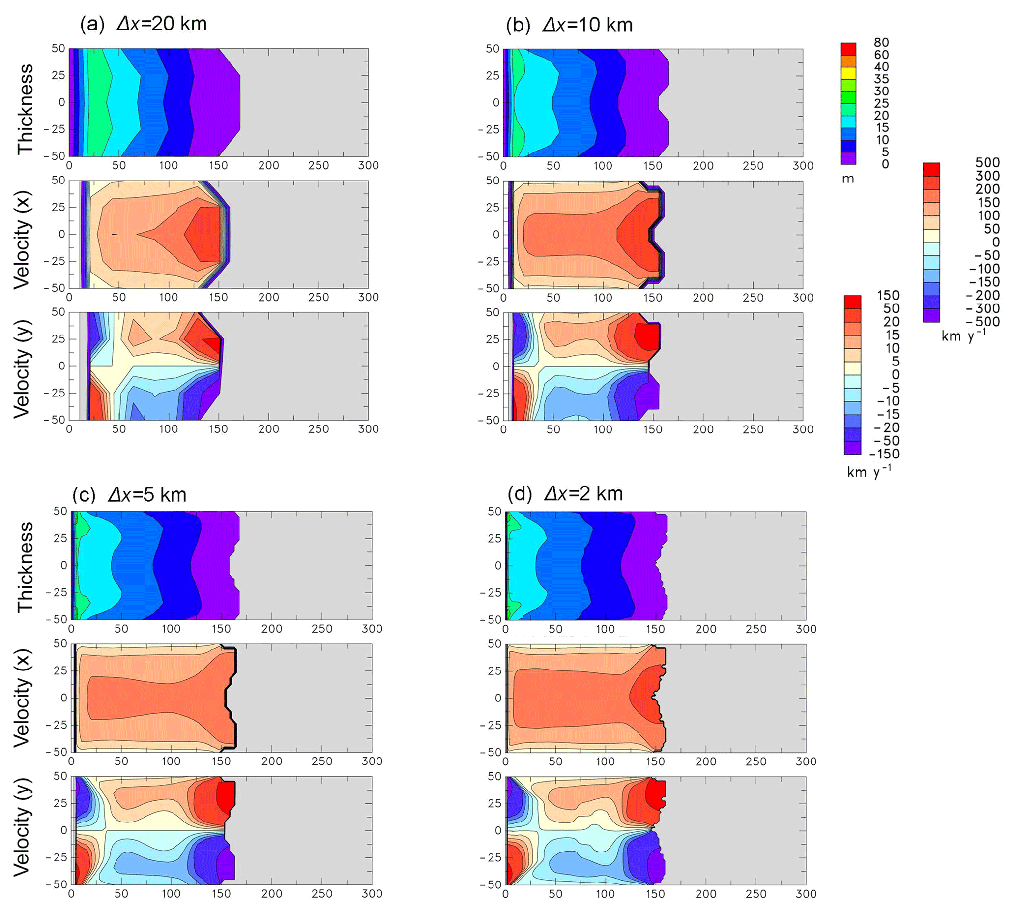
https://www.geosci-model-dev.net/11/5149/2018/gmd-11-5149-2018-f02

Figure 2Same as Fig. 1a (E=10⁶, S=1) but for different model grid sizes. (a) 20 km. (b) 10 km, same as Fig. 1a. (c) 5 km. (d) 2 km.

Download

Table 1Quantities for channel simulations in Fig. 1. Prescribed quantities are as follows: E: flow enhancement factor; n: rheological coefficient; and S: side drag coefficient. Resulting quantities are as follows: ΔF: additional back force on the left-hand ice face due to mélange, compared to that due to ocean water pressure with no mélange, integrated over the width of the channel (see Appendix A); θ_m(left): factor representing degree of buttressing in the mélange, averaged over the left-hand ice face (θ_m= 1 for free flow, ≤ 0 if fully buttressed; see Eqs. A13 and A15); and h_m(left): mélange thickness averaged over the left-hand ice face. The last row shows an additional run with no ocean water drag (β=0 in Eq. 4), so there are no retarding external forces on the mélange at all, for which the resulting ΔF=0 and θ_m=1 as expected.

Download Print Version | Download XLSX

https://www.geosci-model-dev.net/11/5149/2018/gmd-11-5149-2018-f03

Figure 3Maps of mélange quantities in nested simulations of the Jakobshavn region of West Greenland with the coupled ice–mélange model, for three different mélange parameter settings. Flow is right to left. White regions are grounded ice sheet, with a small ice shelf tongue in the southeastern corner of the fjord head. Dark grey regions are ice-free land or inland lakes, and light grey is ocean (Disko Bay and mélange-free fjord water except in the bottom row). Axis tick marks are roughly 10 km apart. (a) With E=10⁶, H_n(H_p)=30(60) and n=5 (near-best-scoring run in the ensemble below). (b) With E=10⁴, H_n(H_p)=60(100) and n=10 (another relatively realistic run). (c) With E=10¹, H_n(H_p)=150(200) and n=1(very stiff and thick mélange). (d) With E=10⁸, H_n(H_p)=10(30) and n=1 (very weak and thin mélange). Top row: mélange thickness (m). Second row: westward velocity (km yr⁻¹). Third row: northward velocity (km yr⁻¹). Bottom row: rate of mélange generation due to ice calving and/or cliff failure, supplied only to mélange grid boxes adjacent to ice faces (meters per year of mélange thickness, M in Eq. 7).

Download

4.2 Jakobshavn fjord

The modern state of mélange and ice in the Jakobshavn fjord of West Greenland is used as a basic calibration of the model. This exercise is not intended as a full-blown modeling study of Jakobshavn, not least because the model resolution of 2 km barely resolves lateral fjord features. The intent here is just to establish very rough constraints on important mélange parameters, with a resolution barely resolving the geometry of interest as in the simulations of Antarctic basins in the next section.

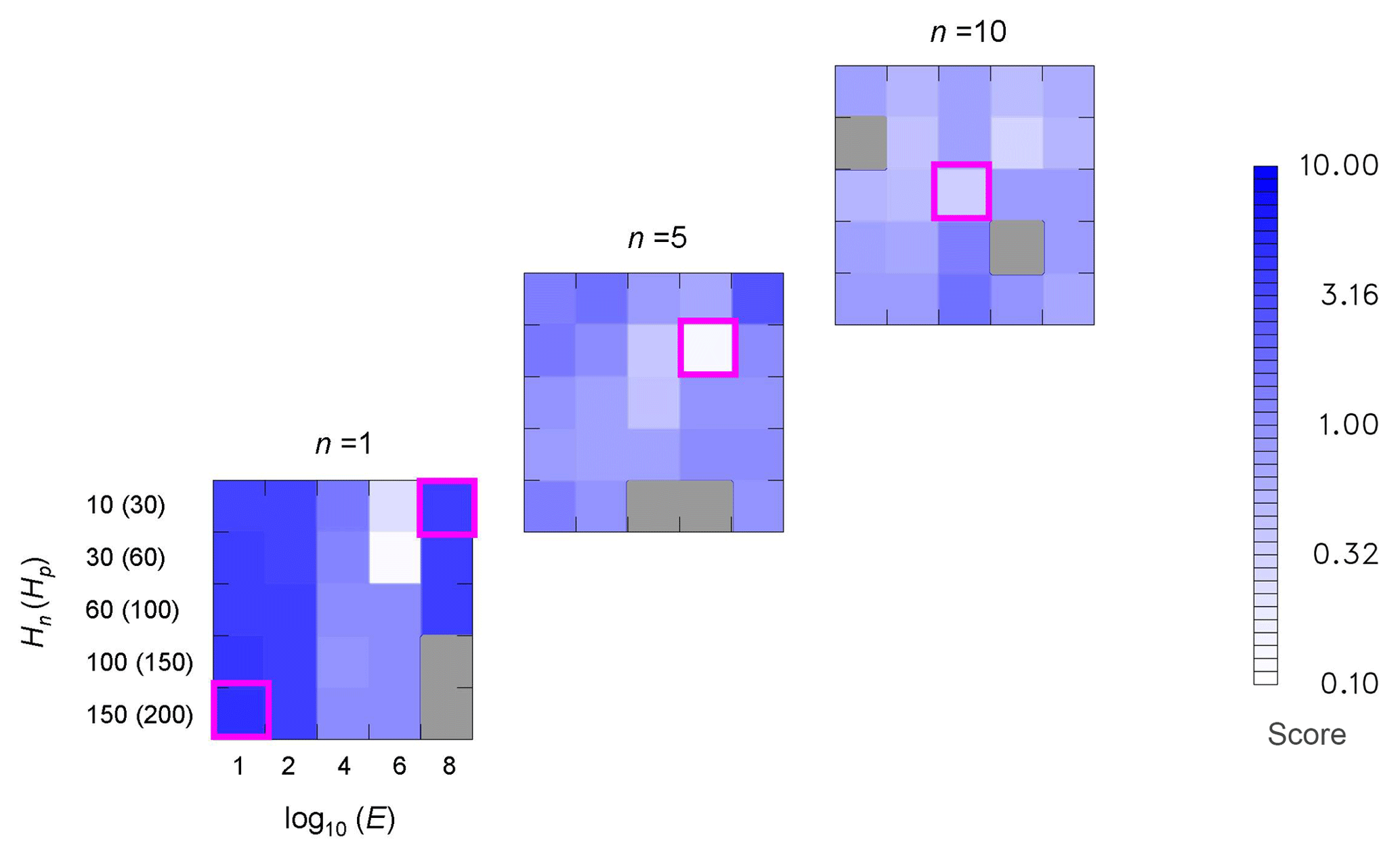
https://www.geosci-model-dev.net/11/5149/2018/gmd-11-5149-2018-f04

Figure 4Scores for all runs in the ensemble of Jakobshavn simulations. Scores of 0 to ∼0.3 indicate rough agreement with observed magnitudes of mélange thicknesses, velocities and extent, and scores of ∼0.5 and greater indicate somewhat to very unrealistic simulations (see Appendix C). Each square with five by five tiles shows scores for ranges of flow enhancement factor E (horizontal axis, 10¹ to 10⁸) and matched pairs of new-mélange and pressure-scaling thicknesses H_n and H_c (vertical axis, meters). The three squares show three values of the rheological coefficient n (bottom left to top right; n=1, 5 and 10). Tiles towards the bottom left correspond to stiffer and thicker mélange, and those towards the top right correspond to weaker and thinner mélange. Grey tiles indicate simulations that encountered numerical instability (see text). Magenta outlines identify the simulations shown in Fig. 3.

Download

The coupled ice sheet–shelf–mélange model is run in nested mode (Pollard and DeConto, 2012), over a longitude–latitude region bounded by 68.42–69.92^∘ N, 51.83–47.83^∘ W. This is roughly a 160×160 km rectangle centered on the Jakobshavn fjord and extending far enough to the north, south and east to provide a sufficient buffer from the domain boundaries. The figures below show a zoomed-in subset of the domain over the fjord itself. Lateral ice boundary conditions (ice thickness, velocities and temperatures) at the domain boundaries are provided by a previous simulation of modern continental Greenland (with no mélange component) at 0.1^∘ latitude × 0.2^∘ longitude resolution. The nested runs have a resolution of 0.02^∘ latitude and 0.04^∘ longitude (roughly 2×2 km). Numerical stability is an issue for these higher resolutions. Some regions of parameter space with weak mélange become dynamically unstable, and this becomes more pervasive at 1 km resolution. With 2 km resolution, only a few runs are unstable (as shown below), and there are enough stable simulations to broadly map parameter space and constrain the basic ranges.

The nested model is initialized to the modern ice state interpolated from the continental run and no mélange, and run 50 years to equilibrium. Both for the continental and nested runs, climatological monthly surface air temperatures and precipitation used for surface mass balance are from the RACMO2 (Regional Atmospheric Climate Model; van Angelen et al., 2014), and ocean temperatures for the sub-ice melt parameterization are from Levitus et al. (2012), although the 400 m depth used for water temperatures as in Pollard et al. (2015) may not be as appropriate for Greenland. The modeled ice margins in the upstream Jakobshavn region are reasonably realistic (Bamber et al., 2013), as is the location of the grounding line at the head of the fjord, and mélange is generated both by cliff failure on the northern side and calving of a very small ice shelf on the southern side. The modeled surface mass balance on the Jakobshavn mélange is around −5 m yr⁻¹, mainly due to summer melt, which has an insignificant effect on total downstream mélange flux due to the short residence time in the fjord.

However, further ad hoc adjustments to the ocean sub-ice melting are needed to achieve rough realism in the nested simulations. To keep the grounding line from advancing too far, oceanic basal melting of the ice shelf at the head of the fjord is prescribed to be 200 m yr⁻¹. For mélange, basal ocean melting in the fjord is set to 30 m yr⁻¹, which is near the low end but much less than the high end (∼300 m yr⁻¹) of ranges estimated by Enderlin et al. (2016). As discussed there, fjord waters are stratified by salinity, with near-freezing water at the top, and warmer and more saline waters below penetrating from Disko Bay (Holland et al., 2008; Motyka et al., 2011; Gladish et al., 2015). This vertical temperature gradient should cause more basal melting for larger ice pieces, but here we simply impose a uniform value. As the mélange approaches Disko Bay, basal melting ramps up to 200 m yr⁻¹ (using the arc-to-open-ocean parameterization that modifies Levitus-calculated melt rates; Pollard and DeConto, 2012; Pollard et al., 2015).

The first two experiments in Fig. 3a and b (first two columns of panels) show that rough agreement with the modern Jakobshavn state can be achieved with appropriately chosen mélange parameters. These combinations of parameters produce near-best scoring in the Jakobshavn ensemble shown further below. The overall magnitudes of mélange thicknesses, downstream velocities and east–west extent correspond with observed fjord-wide average values: 50–150 m for thickness (Enderlin et al., 2016), 20–60 km yr⁻¹ for velocities (Sundal et al., 2013; Foga et al., 2014; Enderlin et al., 2016; Burton et al., 2018) and 40–70 km for total length. These observational ranges are discussed further in Appendix C. In most simulations there are small areas where the mélange grounds on bedrock, along the sides of the fjord and at its head, which slightly slow the mélange and increase back stress at the ice face. Simulated downstream centerline velocities accelerate to several tens of kilometers per year at mid-fjord, with faster velocities at the mouth. The net additional back force due to mélange (compared to open water) on solid ice faces at the head of the fjord is 0.25×10¹² N, or 31 kPa averaged over 8.1×10⁶ m³ of ice face, which is comparable to that estimated for the Store Glacier in West Greenland (30–60 kPa; Walter et al., 2012; Todd et al., 2014). Note that the total downstream flux of mélange ( $\sim 0.25 \times 10^{11}$ m³ yr⁻¹) at the head of the fjord is ∼50 % smaller than the observed Jakobshavn basin discharge (Howat et al., 2011, Supplement), mainly as a consequence of under-resolved grounding-zone bathymetry.

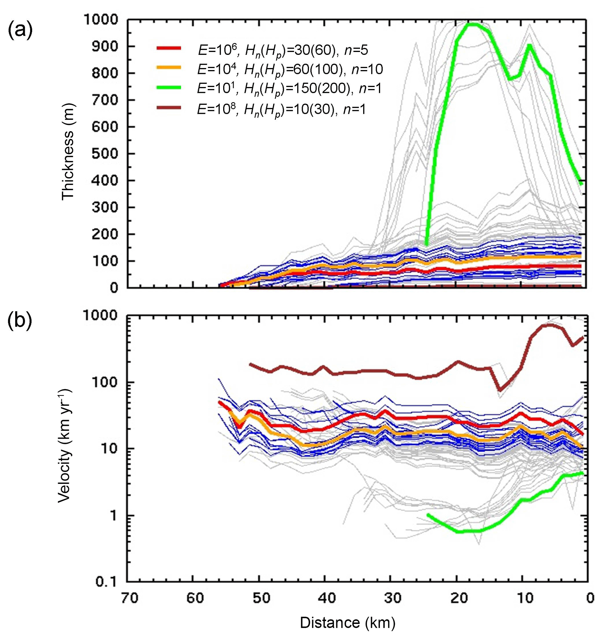
https://www.geosci-model-dev.net/11/5149/2018/gmd-11-5149-2018-f05

Figure 5East–west profiles along the fjord for all simulations in the Jakobshavn ensemble. (a) Mélange thickness (m). (b) Mélange westward velocity (km yr⁻¹). Quantities are averaged over north–south transects across the fjord (as in the scoring calculations, Appendix C). The horizontal axis shows westward distance from the head of the fjord, defined as the most eastward modeled grounding-line location. Red: near-best-scoring run shown in Fig. 3a (E=10⁶, H_n(H_p)=30(60), n=5). Orange: another realistic run shown in Fig. 3b (E=10⁴, H_n(H_p)=60(100), n=10). Green: much stiffer and thicker mélange, shown in Fig. 3c (E=10¹, H_n(H_p)=150(200), n=1). Brown: very weak and thin mélange, shown in Fig. 3d (E=10⁸, H_n(H_p)=10(30), n=1). Blue: runs with the 20 best scores. Grey: all other runs.

Download

Figure 3c (third column) shows an unrealistic simulation, in which the mélange viscosity and new and pressure-scaling mélange thickness values have been increased, and n set to 1, which produces much stiffer and thicker mélange. Mélange thicknesses are ∼1000 m, and the mélange becomes grounded nearly everywhere on the fjord bed, extending only ∼25 km down the fjord. As a consequence of the increased viscosity and basal drag, centerline velocities are only ∼1 to 3 km yr⁻¹. The constricted flow produces a bulging of thickness downstream from the grounding line that relies on along-flow stresses in the SSA equations (Eq. 4) to maintain westward velocities.

The opposite unrealistic situation is shown in Fig. 3d (last column), with greatly reduced viscosity, very thin new and scaling mélange thickness values, and n=1. The mélange is only a few meters thick, and downstream velocities are several hundred kilometers per year. Because of the greatly reduced back pressure on the ice face, the grounding line has retreated about 10 km into the interior at the northeastern end of the fjord.

To efficiently map out the simulated Jakobshavn behavior over parameter space, we performed an ensemble of simulations for all combinations of ranges of three selected mélange parameters: viscosity (via enhancement factor E in Eq. 2), thickness of newly created mélange H_n in Eq. (B3) (matched with H_p in Eq. 5) and rheological exponent n in Eq. (2). Each simulation is run for 50 years to equilibrium as above, 75 runs in all. For each simulation, a score is computed that very roughly represents the realism of the result, combining average departures from observed magnitudes of mélange thicknesses, velocities and extent in the modern fjord. Details of the scoring calculation are described in Appendix C.

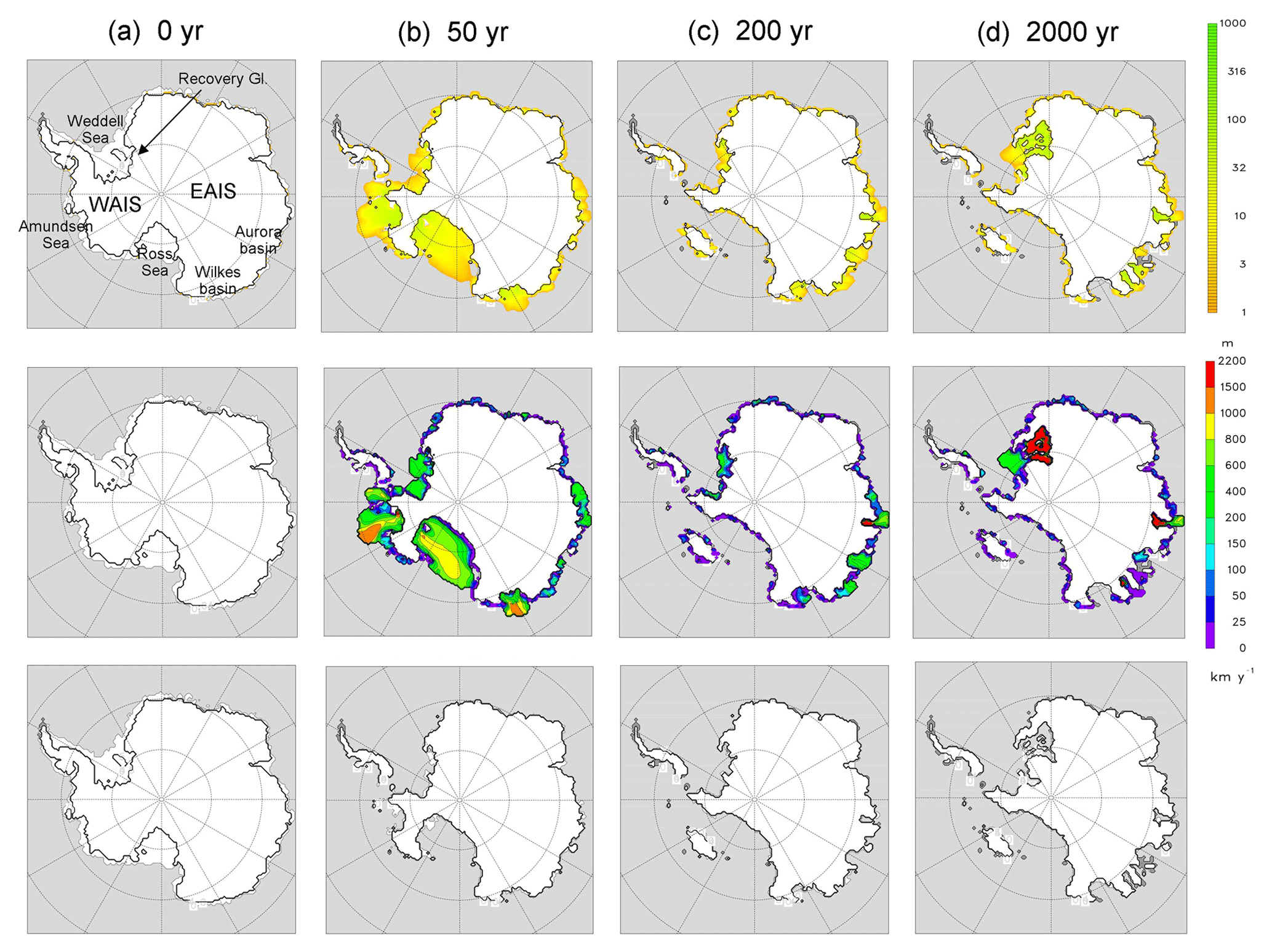
https://www.geosci-model-dev.net/11/5149/2018/gmd-11-5149-2018-f06

Figure 6Snapshots of mélange thickness (m, upper row) and speed (km yr⁻¹, middle row) in a simulation of Antarctic ice retreat, at selected times after a step-function transition from modern to warm mid-Pliocene climate. White regions are solid ice sheet or shelf, grey is ocean and the grounding line is shown by a black line. Mélange parameter values are as in the near-best-scoring run of the Jakobshavn ensemble shown in Fig. 3a (E=10⁶, H_n(H_p)=30(60), n=5). Bottom row shows solid-ice extents from a corresponding simulation with no mélange. (a) 0 yr (modern). (b) 50 yr. (c) 200 yr. (d) 2000 yr. The first panel shows locations of features named in the text; EAIS: East Antarctic Ice Sheet; WAIS: West Antarctic Ice Sheet.

Download

The score results for the whole ensemble are shown in Fig. 4. Realistic results (low scores) are achieved within fairly narrow ranges of enhancement coefficient (E∼10⁴ to 10⁶) and thickness scales (H_n∼30 to 60, H_p∼60 to 100), but for a wide range of rheological exponent (n∼1 to 10). Outside these ranges of E and H_n(H_p), the modeled mélange is generally much too thick and slow as in Fig. 3c, or much too thin and fast as in Fig. 3d. The along-fjord profiles of modeled mélange thickness and velocity in Fig. 5 illustrate the wide range of results, and how reasonable magnitudes are only obtained for limited ranges of parameter values.

4.3 Antarctica

We now use the coupled model to examine the role of mélange during rapid retreat of Antarctic ice. Starting from the ice sheet model state equilibrated to modern climate (with no mélange), an instantaneous change to a warm mid-Pliocene (∼3 Ma) climate is imposed. As described in Pollard et al. (2015), atmospheric forcing is provided by a regional climate model with a warm austral-summer orbit and atmospheric CO₂ level of 400 ppm, and circum-Antarctic ocean temperatures are assumed to warm 2 ^∘C above modern climatology. The inclusion of hydrofracturing and cliff-failure mechanisms in the ice model produces very rapid West Antarctic Ice Sheet (WAIS) retreat within ∼200 years, and major East Antarctic Ice Sheet (EAIS) retreat in the Wilkes, Aurora and Recovery marine basins within ∼3000 years (Pollard et al., 2015). Similar retreat occurs in future model simulations with the IPCC business-as-usual RCP8.5 greenhouse-gas scenario (DeConto and Pollard, 2016). The same ice model version as in those studies is used except for (i) no lapse-rate adjustment to precipitation for the difference between climate-model and ice-model surface elevations, and (ii) an increase of maximum cliff erosional rate from 3 to 12 km yr⁻¹ (more like Jakobshavn today), both of which tend to increase marine ice retreat.

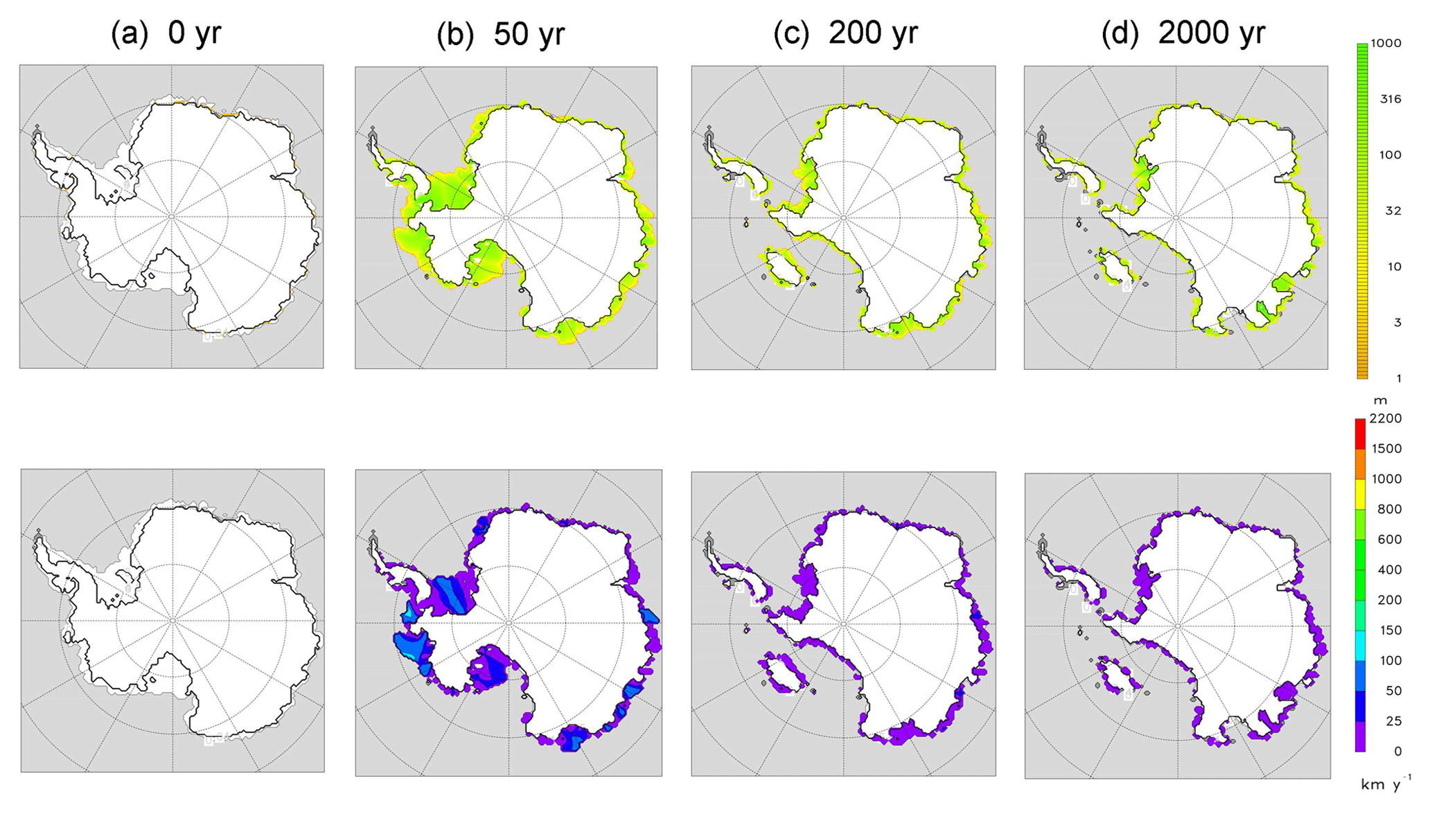
https://www.geosci-model-dev.net/11/5149/2018/gmd-11-5149-2018-f07

Figure 7As Fig. 6 but for parameter values producing very stiff and thick mélange as in Fig. 3c (E=10¹, H_n(H_p)=150(200), n=1). (a) 0 yr (modern). (b) 50 yr. (c) 200 yr. (d) 2000 yr.

Download

As mentioned above, the very fast mélange speeds in some regions and times (up to ∼2000 km yr⁻¹) require very short time steps ( $Δ t < Δ x / 2000$ for numerical stability), and long-term Antarctic runs are only practical at 40 km spatial resolution. Shorter regional tests at higher resolutions (with one example shown below) and the idealized tests in Fig. 2 suggest that the results are reasonably independent of model resolution.

Figure 6 shows snapshots at selected times after the imposition of Pliocene climate, with mélange parameters set to the near-best-scoring values in the Jakobshavn ensemble shown in Figs. 3a and 4 above. Large amounts of mélange are generated within 50 years by retreating ice in marine West Antarctica, producing mélange thicknesses up to 50 m in much of Amundsen and Ross embayments, with lesser thicknesses (∼10 m) in the Weddell. However, the additional back stress of mélange on the ice faces has a negligible effect on WAIS collapse, which occurs almost at the same pace as in the model without mélange (Pollard et al., 2015; Fig. 6 bottom row), and retreat of WAIS marine margins is nearly complete within ∼200 years.

The same is true for later retreat into the major Wilkes, Aurora and Recovery basins of East Antarctica. Despite their more confined and shallow sills, mélange makes very little difference, and retreat into these basins occurs within ∼2000 years as in the model with no mélange. Even with much stiffer and thicker mélange parameters (the combination used in Fig. 3c for Jakobshavn, far outside the realistic range), most of the retreat is largely unaffected, as seen in Fig. 7. West Antarctica and the Wilkes basin still collapse, and retreat is slowed or prevented only in some East Antarctic inlets, notably the Recovery basin east of the Weddell embayment.

Corresponding time series of various quantities are shown for the two cases in Fig. 8. The equivalent global mean sea level (GMSL) for the near-best-scoring parameter values (red curve in Fig. 8a) is nearly the same as in the model with no mélange. This is true for several other (we suspect all) combinations of parameters yielding reasonable mélange magnitudes for Jakobshavn in Fig. 4, for which total GMSL rise in these Antarctic simulations remains close to ∼13 m. Note again that the other case with much stiffer mélange (green curve in Fig. 8a) yields very unrealistic results for Jakobshavn. Other mélange quantities are shown in Fig. 8b–e and vary as expected between the two cases. The pronounced rise in total additional back force with very stiff mélange after ∼2200 years (green curve in Fig. 8e) is due to the delayed retreat into a single East Antarctic inlet around 130^∘ E that collapsed well before 2000 years with the more realistic mélange parameters (seen in Fig. 6d vs. 7d).

A nested run over the Wilkes basin was performed as a basic test of model resolution, shown in Fig. 9. This run corresponds in all respects to the Pliocene retreat scenario in Fig. 6 above except with the grid size reduced to 20 km and with lateral boundary conditions at the domain margins fixed to modern ice. The distribution of mélange is slightly different, but very much the same grounding-line retreat into the Wilkes basin occurs as in the continental run.

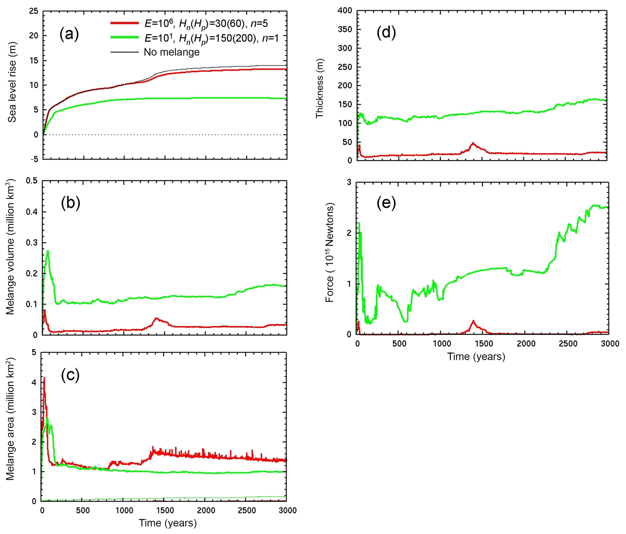
https://www.geosci-model-dev.net/11/5149/2018/gmd-11-5149-2018-f08

Figure 8Time series in simulations of Antarctic retreat after a transition to warm mid-Pliocene climate with two different mélange parameter settings. Red curves: E=10¹, H_n(H_p)=150(200), n=5 (near-best scoring, as in Fig. 6). Green curves: E=10¹, H_n(H_p)=150(200), n=1 (much stiffer and thicker mélange, as in Fig. 7). (a) Equivalent global mean sea level rise (m), with black curve for a corresponding simulation with no mélange. (b) Total mélange volume (10⁶ km³). (c) Total mélange area (10⁶ km²), with thinner curves showing area where grounded. (d) Mélange thickness (m) averaged over all mélange grid cells adjacent to a solid ice face. (e) Total additional back force due to mélange summed over all Antarctic ice faces, compared to that due to ocean water pressure with no mélange (10¹⁵ N; see Appendix A).

Download

https://www.geosci-model-dev.net/11/5149/2018/gmd-11-5149-2018-f09

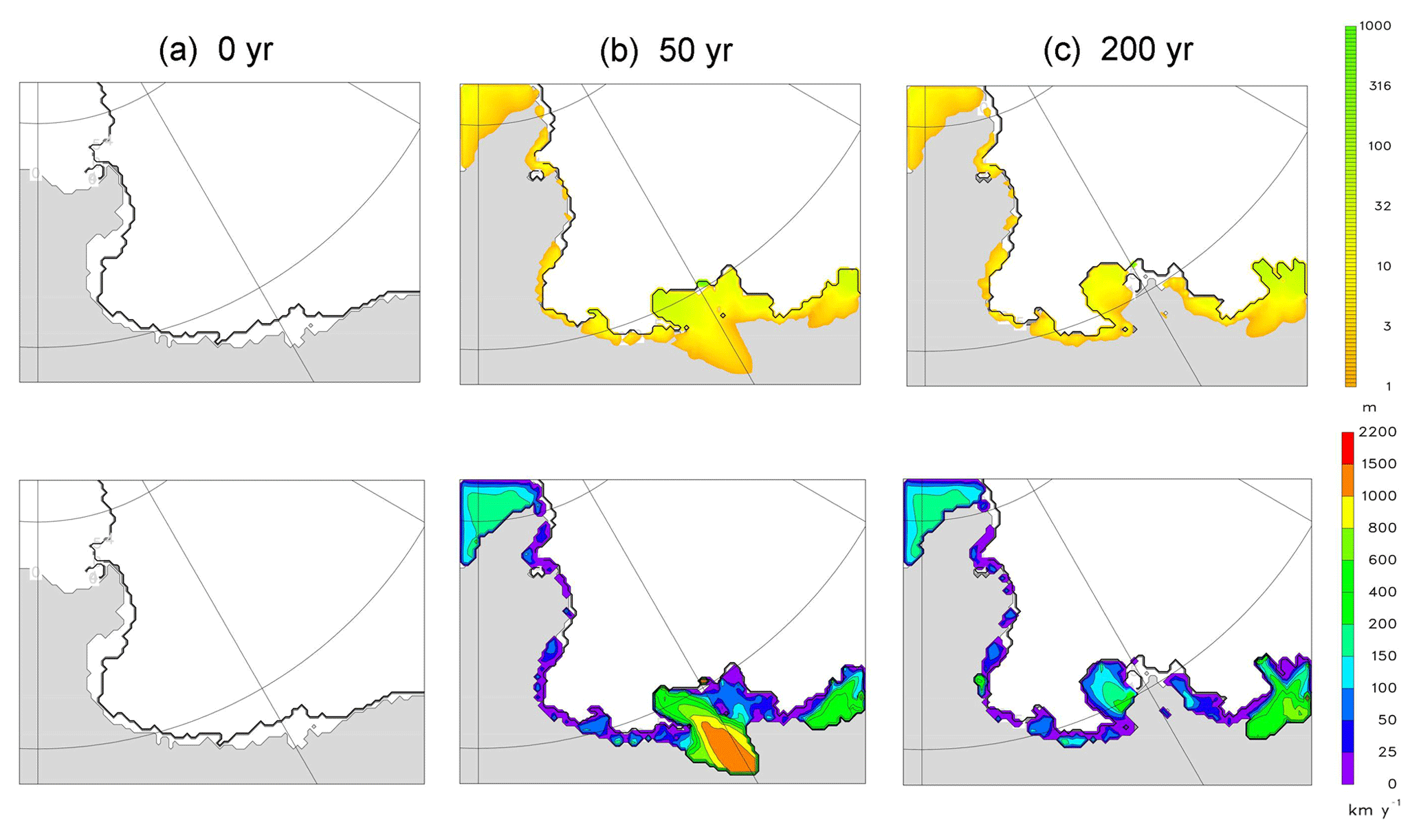
Figure 9Snapshots of mélange thickness (m, upper row) and speed (km yr⁻¹, lower row) in a limited-area nested simulation at 20 km resolution over the Wilkes subglacial basin, East Antarctica, after a step-function transition to warm mid-Pliocene climate. Model parameters are as in Fig. 6, including mélange settings (near-best scoring, E=10⁶, H_n(H_p)=30(60), n=5). (a) 0 yr (modern). (b) 50 yr. (c) 200 yr.

Download

https://www.geosci-model-dev.net/11/5149/2018/gmd-11-5149-2018-f10

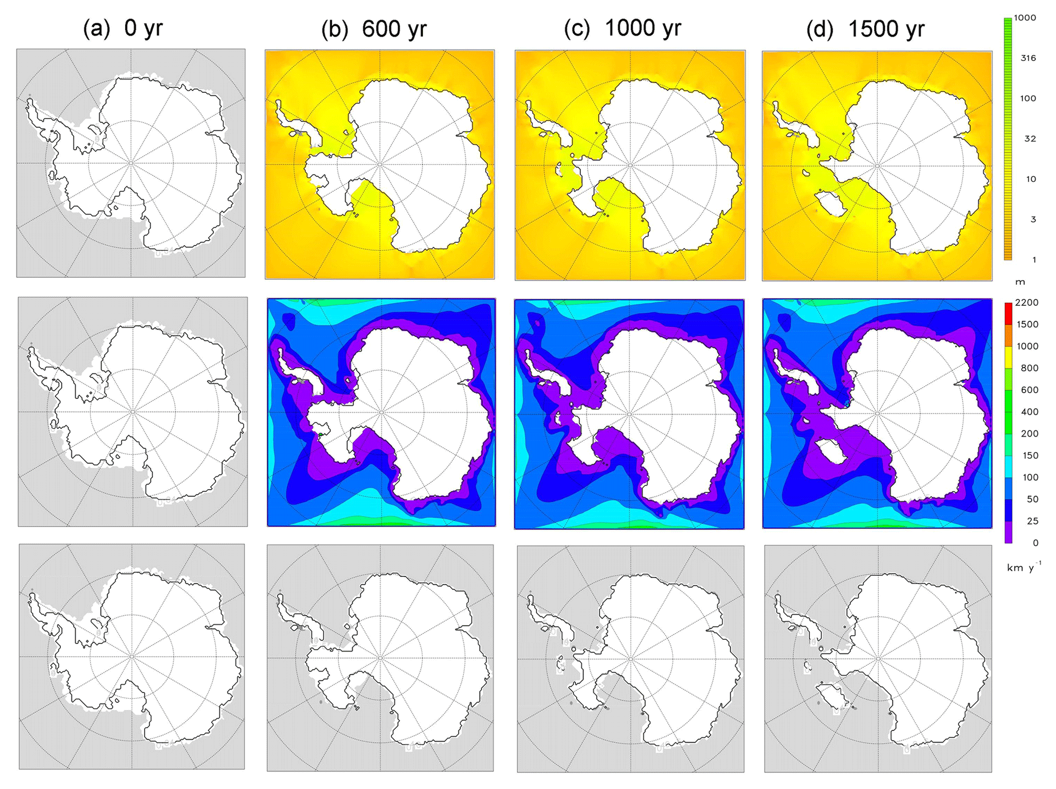
Figure 10As Fig. 6 except with atmospheric and oceanic forcing gradually ramped from modern to mid-Pliocene over the first 300 years. Hydrofracturing and cliff-failure mechanisms are disabled, and surface and oceanic melting of mélange are set to zero (see text). Upper row: mélange thickness (m). Middle row: mélange speed (km yr⁻¹). Bottom row: solid-ice extents in a corresponding simulation with no mélange. Note the different times from those in Fig. 6.

Download

4.4 Slower Antarctic retreat

In the above simulations, the rate of Antarctic ice retreat is very large, due to the added mechanisms of hydrofracturing and cliff failure, producing marine ice cliff instability. These mechanisms drastically attack the solid ice and may overwhelm any retarding effect of mélange. Also, the transition to warm mid-Pliocene atmospheric and oceanic forcing imposed above as an abrupt step function at the start of the run causes melting of the mélange as well as ice, and so it significantly thins the mélange faster than a more gradual warming would. Here we examine the role of mélange in scenarios with slower ice retreat and more gradual warming, similar to the retreat found in other studies without hydrofracturing and mélange. In those studies, West Antarctic marine ice still collapses in past and future (business as usual) warm climates, driven primarily by increased sub-ice-shelf melting and marine ice sheet instability, but the collapse is considerably slower, taking O(1000) years compared to O(100) years (Pollard and DeConto, 2009; Feldmann and Levermann, 2015; Golledge et al., 2015; Winkelmann et al., 2015). The nominal Antarctic simulation above (Fig. 6) is modified by

disabling the hydrofracturing and cliff-failure mechanisms;
imposing a gradual linear ramp in atmospheric and oceanic warming, from modern to warm mid-Pliocene over the first 300 years of the simulation;
setting all atmospheric and oceanic melting of mélange to zero.

The results are shown in Fig. 10. As expected, initial West Antarctic retreat is delayed, beginning in earnest after 500 years and taking ∼1500 years to complete, much longer than in Fig. 6. Unlike Fig. 6, ice shelves persist in West Antarctica during the early phase (Fig. 10, 600 years). Also as expected and unlike Fig. 6, without the hydrofracturing and cliff-failure mechanisms, major East Antarctic basins do not undergo collapse (Pollard et al., 2015). Despite the slower West Antarctic retreat and despite mélange (unrealistically) being unaffected by local melt and occupying the entire oceanic domain, there is still negligible slowdown compared to a corresponding simulation with no mélange (bottom row, Fig. 10). The same is true if local melting of mélange is allowed, which limits mélange extent to very small areas, and ice retreat is almost the same as in Fig. 10 (not shown). Hence, the same basic behavior as found above still occurs in scenarios with slower MISI-driven retreat: mélange produces negligible back stress and retardation of retreating Antarctic ice fronts.

5 Conclusions

A continuum-mechanical model of mélange has been formulated that is computationally feasible for continental spatial and multi-millennial timescales. In idealized channel tests it captures basic dependencies between supply rate, flow, side drag and ocean bottom resistance, and their influence on back pressure on ice faces. The model behaves consistently over a wide range of grid sizes.

The model was tested in simulations of mélange in the Jakobshavn fjord, West Greenland, aiming to calibrate the main uncertain model parameters for viscosity, side drag and bedrock drag. Ranges of these parameters are found that yield roughly correct magnitudes of mélange thickness, velocity and extent; values outside these ranges yield very unrealistic results with excessive thicknesses (for stiffer values) or excessive speeds (for weaker values).

When applied to rapid Antarctic retreat events using warm mid-Pliocene climate as an example, the inclusion of mélange has little effect on the response of Antarctic ice for parameter values that yield reasonable Jakobshavn simulations. Extensive ∼50 m thick mélange covers the Amundsen and Ross embayments in the early stages, with thinner mélange in the Weddell, but the additional back pressure on the retreating ice faces does not slow down the retreat noticeably, and marine WAIS collapse still occurs within ∼200 years. The same is true for later retreat into the major marine basins of East Antarctica, despite their narrower and shallower sills. The lack of influence of mélange is a consequence of the huge spatial scales of Antarctic ice fronts and seaways compared to Greenland fjords, and almost unimpeded spreading of mélange into the Southern Ocean. This behavior is consistent with Burton et al. (2018) finding that mélange back stress increases exponentially with increasing L∕W and is capable of inhibiting calving for $L / W > \sim 3$ , where L∕W is the ratio of mélange length to width in the confining channel. Here, L∕W is ∼5 for Jakobshavn (Fig. 3a, b) and close to 0 for the resolved embayments of Antarctica.

Mélange still has a negligible effect on West Antarctic retreat if the mechanisms of hydrofracturing and cliff failure are removed, and climate warming is imposed more gradually. In that case WAIS collapse still occurs due to increased oceanic sub-ice-shelf melt and marine ice sheet instability, but more slowly on ∼ thousand-year timescales, as in other models. To produce significant slowdown of Antarctic retreat in any of our simulations, mélange parameters must be set to much “stiffer” values, far outside the reasonable ranges for Jakobshavn. Even then, retreat is slowed or prevented only for some East Antarctic basins (notably the relatively restricted Recovery basin), and still occurs in West Antarctica and the Wilkes basin.

Within the framework of this study, the results strongly indicate that mélange has very little influence on major Antarctic ice retreat. However, the model clearly has large uncertainties. Even though it produces reasonable magnitudes of some mélange properties in Jakobshavn, that does not mean that the dynamical processes in the model accurately represent mélange there. Even if they do, their applicability to the much larger scales of Antarctica would still be questionable. One primary need is detailed mechanistic models of calving and cliff failure, to replace the simple empirical parameterizations currently used. Mélange may have greater effects in more mechanistic models of calving, for instance in preventing overturning of icebergs (Amundson et al., 2010, their Fig. 9, where the required mélange forces, O(10⁷ to 10⁸) N m⁻¹, are comparable to those in our Jakobshavn simulations). Another hopeful goal is to link the results of discrete-particle models of mélange with continuum descriptions as here. Beyond that, the following steps are planned for future work.

Using higher resolution in Jakobshavn simulations, and performing more detailed and thorough calibration to modern observations. This would include seasonal variations due to winter freezing and hardening of the mélange by the sea ice matrix, which prevents calving during winter (Joughin et al., 2008, 2014b; Amundson et al., 2010). With seasonal variations, an additional rheologic term may be desirable to prevent unrealistic deformation at thin oceanic edges during summer, as in sea ice modeling (Hibler, 2001; Leppäranta, 2012), but it is unclear if this should also apply to mélange.
Simulating past variations of Jakobshavn ice and mélange extents, during the Holocene, the last two centuries and recent decades (Csatho et al., 2008; Joughin et al., 2008; Young et al., 2011).
Improving the numerical treatment of the ice–mélange junction when it migrates across multiple grid cells. As described in Appendix B, this is done simply but not rigorously in the current model, and would involve fractional grid coverage for mélange, which is not yet in the model as it is for ice shelves (although no detrimental behavior has been seen to date; cf. Albrecht et al., 2011).
Distinguishing between supply of mélange vs. large tabular bergs in the ice model's calving parameterization (Pollard and DeConto, 2012). For modern Antarctica, model calving at the edges of the Ross and Weddell shelves produces a small amount of mélange, contrary to observations (but has very little effect on the model's modern state).
Allowing depth-dependent oceanic melt rates, appropriate for thick mélange in marine settings with steep vertical temperature gradients.
Including mélange transport by ocean currents, particularly the circum-Antarctic western boundary current that today advects most icebergs counterclockwise around the Antarctic coast and then northwards off the eastern Antarctic Peninsula (Weber et al., 2014). Similar routing could influence the huge amounts of mélange generated during rapid retreat episodes.

Code and data availability

Selected output files, metadata and model code are available at Penn State's Data Commons (http://www.datacommons.psu.edu/commonswizard/MetadataDisplay.aspx?Dataset=6172, https://doi.org/10.18113/D3KQ19, Pollard et al., 2018).

Appendix A: Mélange back stress

This appendix describes the force balance on ice shelves and mélange, as entities separate from grounded ice. The analysis is based on the net force on any of these bodies being essentially zero at any time. Appendix B describes kinematic relationships involving the conversion of ice to mélange across the ice–mélange interface, based on conservation of mass. Both appendices derive equations that are used in the model as boundary conditions.

Back stress by mélange in contact with vertical solid ice faces is computed in the model. This can occur either at the grounding line of marine ice cliffs with no ice shelf (tidewater termini) or at the outer edge of floating ice shelves. The back stress stems from the net forces on the mélange that resist downstream flow, i.e., side drag or blockage by land or ice, basal drag if the mélange grounds on ocean bedrock rises, and (relatively small) friction between the mélange base and ocean water. The process is much the same as the well-known buttressing at grounding lines by ice shelves, but analysis is slightly more complicated because the mélange only occupies a part of the vertical ice face, and the junction is between two separate bodies, not within contiguous ice. Stretching forces are not transmitted across the boundary, and $\partial u / \partial x$ in the ice may be different from that in the mélange adjacent to the boundary (it is continuous across sheet–shelf grounding lines). The simpler ice shelf case is reviewed first in Sect. A1, and the mélange case is analyzed in Sect. A2, leading to the expression for mélange back stress used in the model.

The treatment below is for 1-D flow lines in the x direction, with no transverse variation. We note below (after Eq. A2) how some expressions would be modified for transverse variability in the y direction, still with the grounding line running perpendicular to the x axis.

A1 Ice shelf back stress at a grounding line

Buttressing by an ice shelf of grounded ice flowing across the grounding line is accounted for in our existing ice sheet model by the term θ in the equation for grounding-line ice velocity (Schoof, 2007, his Eq. (29); equal to τ_xx∕τ_f; Pollard and DeConto, 2012, their Eq. 8). θ is the ratio of the longitudinal deviatoric stress at the grounding line to its value if the ice shelf were completely unconfined or did not exist. As in SSA scaling, vertical shear is neglected in the vicinity of and downstream of the grounding line, and all main quantities here are independent of height.

\begin{matrix} (A1) & θ = (4 η \frac{\partial u}{\partial x}) / (4 η \frac{\partial u_{f}}{\partial x}), \end{matrix}

where the effective viscosity η is given by Eq. (2) of the main text (with n=3). The reason for the factor 4 (which cancels in Eq. A1) is mentioned following Eq. (A2) below.

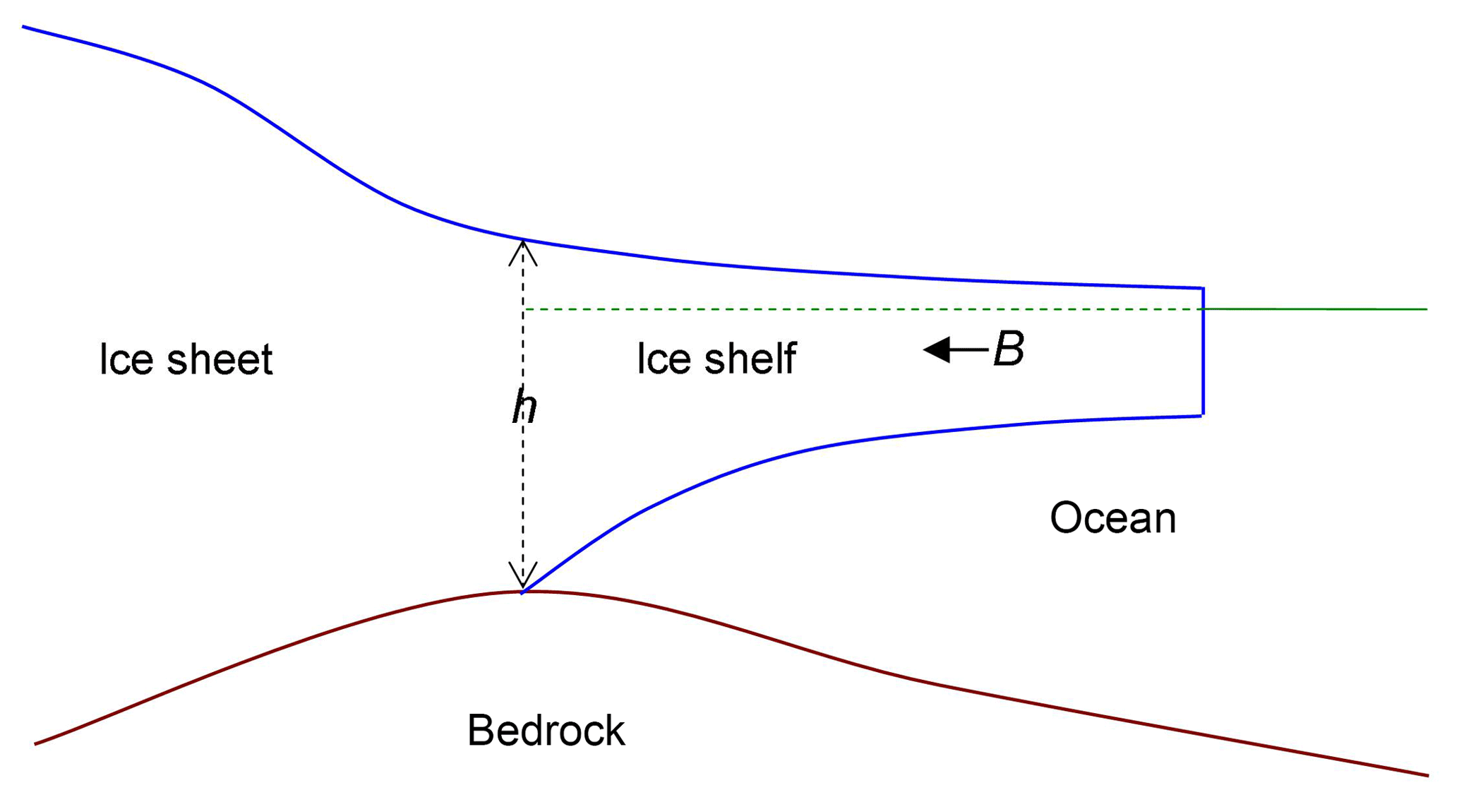
https://www.geosci-model-dev.net/11/5149/2018/gmd-11-5149-2018-f11

Figure A1Schematic of an ice sheet and ice shelf at the grounding line. B is the net backward force on the ice shelf due to side drag or grounding on bedrock.

Download

Referring to the schematic in Fig. A1, the net force (towards the right, vertically integrated, per unit length in the transverse direction) on the entire ice shelf must be zero; it is

\begin{matrix} (A2) & - 4 η \frac{\partial u}{\partial x} h + \frac{ρ_{i} g h^{2}}{2} - \frac{ρ_{w} g}{2} {(\frac{ρ_{i}}{ρ_{w}} h)}^{2} - B = 0 . \end{matrix}

Note that the extra factor of 2 in the 4η term at the start of Eq. (A2), instead of 2η, comes from the effect of vertical deviatoric stress 2 $η \partial w / \partial z$ in the vertical force balance with gravity (e.g., Thoma et al., 2014). For two horizontal dimensions (with the grounding line still perpendicular to the x axis), the first term in Eq. (A2) would be 2 $η (\partial u / \partial x + (\partial u / \partial x + \partial v / \partial y))$ h, as in the SSA equations for velocity u (seen for mélange in Eq. 4a). For the two-dimensional case, wherever 4 $η \partial u / \partial x$ appears in this Appendix, it should be replaced by 2η(2 $\partial u / \partial x + \partial v / \partial y)$ , including the subscripted terms 4 $η_{i} \partial u_{i} / \partial x$ and 4 $η_{m} \partial u_{m} / \partial x$ for ice and mélange separately in the next subsection.

If the shelf is freely floating (or non-existent), B=0 in Eq. (A2), and the unconfined strain rate $\partial u_{f} / \partial x$ is given by

\begin{matrix} (A3) & - 4 η \frac{\partial u_{f}}{\partial x} h + \frac{ρ_{i} g h^{2}}{2} - \frac{ρ_{w} g}{2} {(\frac{ρ_{i}}{ρ_{w}} h)}^{2} = 0 . \end{matrix}

Using Eq. (A1),

θ = (4 η \frac{\partial u}{\partial x} h) / (\frac{ρ_{i} g h^{2}}{2} - \frac{ρ_{w} g}{2} {(\frac{ρ_{i}}{ρ_{w}} h)}^{2})

i.e.,

\begin{matrix} (A4) & θ = (4 η \frac{\partial u}{\partial x} h) / (\frac{ρ_{i}^{'} g h^{2}}{2}), \end{matrix}

where $ρ_{i}^{'} = (1 - ρ_{i} / ρ_{w}) ρ_{i}$ . Equation (A4) is the expression used for θ in our ice sheet–shelf model, with $\partial u / \partial x$ obtained iteratively from the model's velocity solution (Pollard and DeConto, 2012; Pollard et al., 2015; DeConto and Pollard, 2016).

The following relation, although not used in the model, clarifies the connection between θ and the net external forces B resisting ice shelf flow downstream (basal pinning points, side drag and/or blockage). Combining Eqs. (A2) and (A4) yields

\begin{matrix} (A5) & θ = 1 - \frac{B}{(ρ_{i}^{'} g h^{2} / 2)} . \end{matrix}

So with B=0, i.e., an unconfined or non-existent ice shelf, θ=1. As B increases, θ decreases and reaches 0 when $B = ρ_{i}^{'} g h^{2} / 2$ , i.e., when the combination of B and total water pressure on the ice shelf exactly balances the column-integrated hydrostatic pressure at the grounding line, and stretching $\partial u / \partial x$ at the grounding line is zero (from Eq. A2).

A2 Mélange back stress at a tidewater cliff or an ice shelf edge

The analysis of mélange back stress is similar to the above but is more involved because (i) the mélange occupies only a portion of the vertical ice face and (ii) the junction is between two distinct bodies, so longitudinal stress is not transmitted across it.

Just as for ice shelf buttressing above, θ_i is the ratio of longitudinal strain in the solid ice adjacent to the mélange, relative to what it would be with no mélange:

\begin{matrix} (A6) & θ_{i} = (4 η_{i} \frac{\partial u_{i}}{\partial x}) / (4 η_{i} \frac{\partial u_{if}}{\partial x}) . \end{matrix}

Unlike the ice shelf case, this applies to solid ice immediately upstream of the face. The subscript “i” indicates solid-ice quantities, and subscript “m” below indicates mélange quantities. θ_i is used by the ice sheet model to account for mélange back stress, just as θ from Eq. (A4) is used for ice shelf back stress. Note that throughout this section the mélange viscosity η_m includes the factor f for mélange convergence or divergence, i.e., η_m=fη, where η is given by Eq. (2).

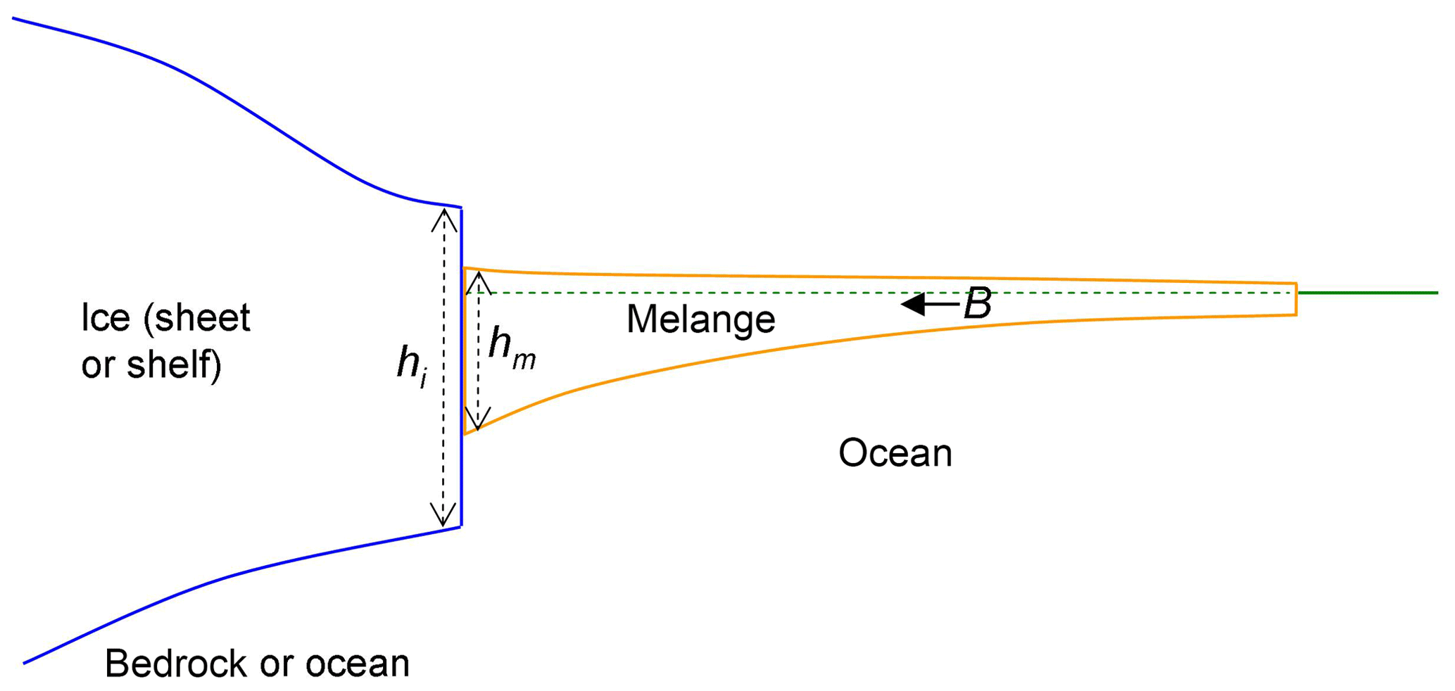
https://www.geosci-model-dev.net/11/5149/2018/gmd-11-5149-2018-f12

Figure A2Schematic of mélange at the vertical face of an ice sheet or ice shelf. B is the net backward force on the mélange due to side drag, grounding on bedrock, or blocking ice further downstream.

Download

Referring to Fig. A2, the leftward force F_m exerted by the mélange on the ice face (the portion of the ice face that it touches), equal to the rightward force exerted by the ice on the mélange, is

\begin{matrix} (A7) & F_{m} = - 4 η_{m} \frac{\partial u_{m}}{\partial x} h_{m} + \frac{ρ_{m} g h_{m}^{2}}{2} + P_{p} . \end{matrix}

P_p is the vertically integrated pressure term representing packing given by Eq. (5). ρ_m is the bulk density of mélange, which may be slightly greater than ice density ρ_i due to embedded liquid within the mélange. As noted for ice after Eq. (A2) above, the first term on the right in Eq. (A7) with longitudinal stretching $\partial u_{m} / \partial x$ enters not because of any direct stretching or compression of the ice but because of the modification to hydrostatic pressure in the mélange adjacent to the ice, via the effect of deviatoric stress 2 $η_{m} \partial w_{m} / \partial z$ in the vertical force balance.

The net force (towards the right) on the entire body of mélange must be zero; it is

\begin{array}{l} (A8) & F_{m} - \frac{ρ_{w} g}{2} {(\frac{ρ_{m}}{ρ_{w}} h_{m})}^{2} - B \\ = - 4 η_{m} \frac{\partial u_{m}}{\partial x} h_{m} + \frac{ρ_{m} g h_{m}^{2}}{2} - \frac{ρ_{w} g}{2} {(\frac{ρ_{m}}{ρ_{w}} h_{m})}^{2} - B + P_{p} \\ = 0, \end{array}

which also follows by integrating Eq. (4a) in the x direction from an open-ocean boundary to the grounding line, using the open-ocean boundary condition Eq. (6) and with B representing the integrated basal friction. B can also include side friction arising from the second term on the left of Eq. (4a) (involving $\partial u_{m} / \partial y$ ) if it is also integrated in the y direction between walls running parallel to the x axis.

Similarly, the net force (towards the left) on the solid ice face, due both to the mélange contact and the hydrostatic pressure of ocean water, is

\begin{matrix} (A9) & F_{i} = F_{m} + \int_{\frac{ρ_{m}}{ρ_{w}} h_{m}}^{\frac{ρ_{i}}{ρ_{w}} h_{i}} ρ_{w} g z d z . \end{matrix}

And this must be in balance with the rightward force on the vertical face in the ice immediately upstream, so F_i also obeys

\begin{matrix} (A10) & F_{i} = \frac{ρ_{i} g h_{i}^{2}}{2} - 4 η_{i} \frac{\partial u_{i}}{\partial x} h_{i} . \end{matrix}

Combining Eqs. (A6) and (A10),

\begin{matrix} (A11) & θ_{i} = \frac{(ρ_{i} g h_{i}^{2} / 2) - F_{i}}{(ρ_{i} g h_{i}^{2} / 2) - F_{if}} . \end{matrix}

Using Eqs. (A7) and (A9) in Eq. (A11),

\begin{array}{l} (A12) & θ_{i} = \\ 1 - \frac{(ρ_{m}^{'} g h_{m}^{2} / 2 + P_{p})}{ρ_{i}^{'} g h_{i}^{2} / 2} (1 - \frac{4 η_{m} h_{m} (\partial u_{m} / \partial x)}{(ρ_{m}^{'} g h_{m}^{2} / 2 + P_{p})}), \end{array}

where $ρ_{m}^{'} = (1 - ρ_{m} / ρ_{w}) ρ_{m}$ and $ρ_{i}^{'} = (1 - ρ_{i} / ρ_{w}) ρ_{i}$ . This expression for θ_i is used in the model to account for back pressure by mélange at ice cliff faces (Pollard et al., 2015), as well as to modify the boundary condition in the SSA dynamics at the edges of ice shelves (Pollard et al., 2012) (noting again that η_m includes the factor f for mélange convergence or divergence). Note that Eq. (A12) can be written

1 - θ_{i} = \frac{(ρ_{m}^{'} g h_{m}^{2} / 2 + P_{p})}{ρ_{i}^{'} g h_{i}^{2} / 2} (1 - θ_{m}),

where

\begin{matrix} (A13) & θ_{m} = \frac{4 η_{m} h_{m} (\partial u_{m} / \partial x)}{({ρ^{'}}_{m} g h_{m}^{2} / 2 + P_{p})} . \end{matrix}

θ_m is the factor representing degree of buttressing in the mélange adjacent to the face (θ_m=1 if free flow, θ_m≤0 if fully buttressed) and corresponds to θ_i for ice.

As for the ice shelf case above, additional relationships can be written that, although not used in the model, clarify the connection between θ_i,θ_m and the net external forces B resisting mélange flow downstream (bedrock grounding, side drag and/or blockage). Substituting Eqs. (A8) and (A9) into Eq. (A11) leads to

\begin{matrix} (A14) & θ_{i} = 1 - \frac{B}{(ρ_{i}^{'} g h_{i}^{2} / 2)}, \end{matrix}

\begin{matrix} (A15) & θ_{m} = 1 - \frac{B}{(ρ_{m}^{'} g h_{m}^{2} / 2 + P_{p})} . \end{matrix}

This is exactly the same form as Eq. (A5) for the ice shelf case above (without P_p), and the same discussion applies for mélange. If B and P_p=0, i.e., no downstream external forces on the mélange (except water pressure), then $θ_{i} = θ_{m} = 1$ , and the ice face feels the same force as if no mélange exists. As B increases, θ_mdecreases and reaches 0 when $B = ρ_{m}^{'} g h_{m}^{2} / 2 + P_{p}$ , i.e., when the combination of B and total water pressure on the mélange exactly balances the column-integrated hydrostatic and packing pressure in the mélange adjacent to the solid ice face, and mélange stretching $\partial u_{m} / \partial x$ is zero. Note that at that point θ_i is not necessarily zero. If B is larger, θ_m becomes negative, i.e., the mélange is being compressed immediately downstream of the face with $\partial u_{m} / \partial x < 0$ , which does occur in some of our simulations with large side drag or grounded mélange.

Another quantity of interest is the net force (towards the left) on the solid ice face, due both to the mélange contact and the hydrostatic pressure of ocean water, minus what it would be just due to ocean water pressure in the absence of mélange, i.e, F_i−F_if. Rearranging Eq. (A11), and using $F_{if} = ρ_{w} g (ρ_{i} / ρ_{w})^{2} h_{i}^{2} / 2$ (i.e., Eq. A9 with h_m=0), as well as Eq. (A13), yields

\begin{array}{l} (A16) & F_{i} - F_{if} = & (1 - θ_{i}) \frac{ρ_{i}^{'} g h_{i}^{2}}{2} \\ = & (1 - θ_{m}) (\frac{ρ_{m}^{'} g h_{m}^{2}}{2} + P_{p}) . \end{array}

This expression is used in the model to calculate the total force difference F_i−F_if integrated over all ice faces in contact with mélange, as a diagnostic domain-wide measure of mélange buttressing during a simulation. Another quantity of interest is the leftward force on the ice face exerted by the mélange itself, F_m in Eq. (A7). Combining Eqs. (A7) and (A13),

\begin{matrix} (A17) & F_{m} = (1 - θ_{m}) (\frac{ρ_{m}^{'} g h_{m}^{2}}{2} + P_{p}) + \frac{ρ_{m}^{2} g h_{m}^{2}}{2 ρ_{w}} . \end{matrix}

Similarly, the total leftward force on the ice face due to the mélange and water, F_i in Eq. (A9), is

\begin{matrix} (A18) & F_{i} = (1 - θ_{m}) (\frac{ρ_{m}^{'} g h_{m}^{2}}{2} + P_{p}) + \frac{ρ_{i}^{2} g h_{i}^{2}}{2 ρ_{w}} . \end{matrix}

Appendix B: Ice-to-mélange conversion

This appendix analyzes the relatively narrow zone where solid ice is converted to mélange, at a tidewater face of grounded ice, or the open-ocean edge of an ice shelf. The zone is relatively narrow compared to the grid size, not resolved in the model, and the physics of calving or cliff failure that occur within it are not addressed here (their net rates are parameterized within the ice model). Relations based on conservation of mass are derived that relate the net effect of the conversion to model variables, mainly to provide the correct velocity boundary condition at the face for the mélange SSA velocity equations. Following that, issues with implementation in the model's finite-difference grid are described.

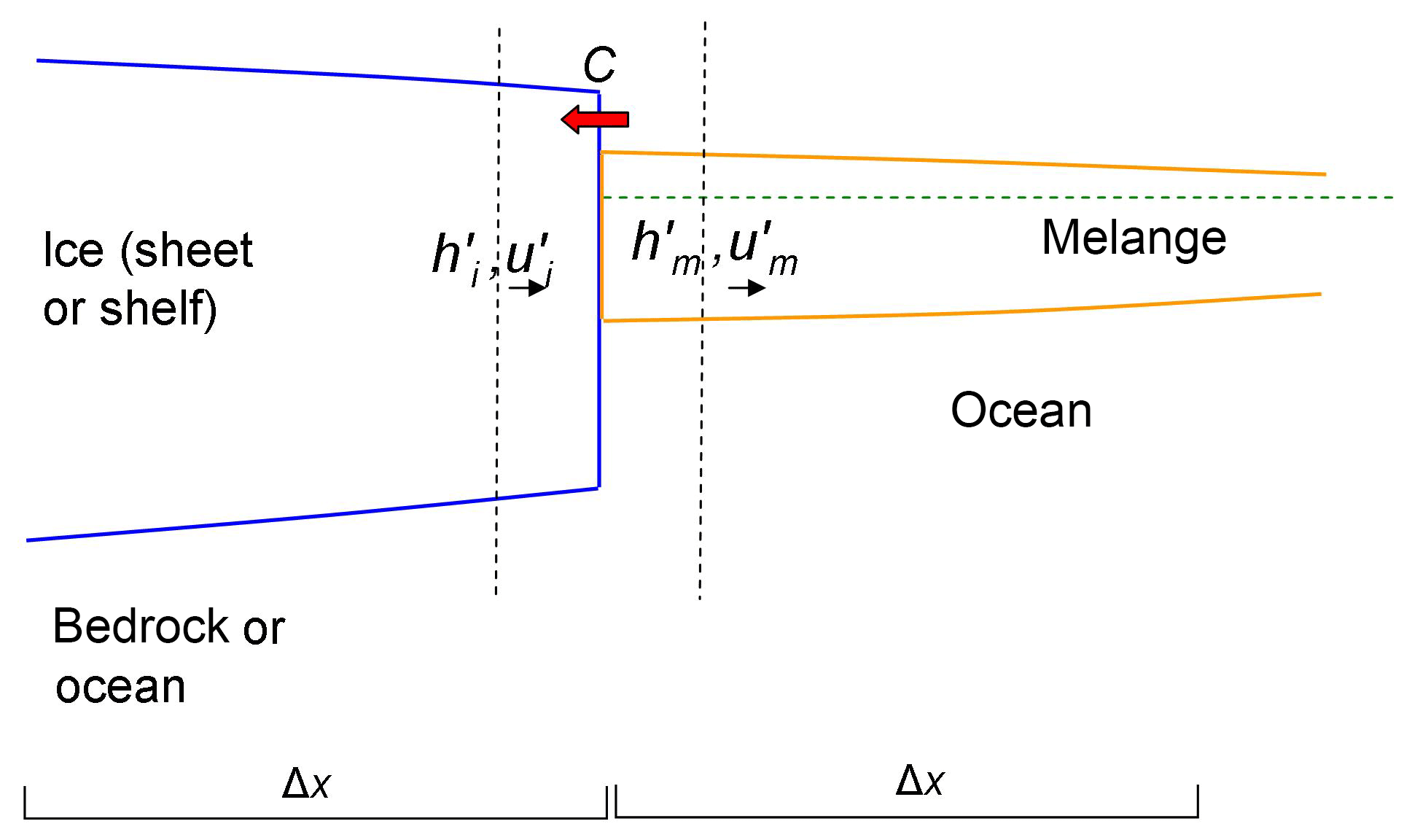
https://www.geosci-model-dev.net/11/5149/2018/gmd-11-5149-2018-f13

Figure B1Schematic of the ice–mélange interface zone (between the two vertical dashed lines), in which new mélange is generated by calving or cliff failure of the ice face. $h_{i}^{'}$ and $u_{i}^{'}$ are the thickness and velocity, respectively, of solid ice just upstream of the ice face, and $h_{m}^{'}$ and $u_{m}^{'}$ are the same for mélange just downstream of the face. C is the rate of cliff or calving erosion horizontally into the ice interior. Two model h-grid cells (Δx) are indicated at the bottom.

Download

Referring to Fig. B1, $h_{i}^{'}$ and $u_{i}^{'}$ are the thickness and velocity, respectively, of solid ice just upstream of the ice face, and $h_{m}^{'}$ and $u_{m}^{'}$ are the same for mélange just downstream of the face. A prime (^′) is used to indicate that these quantities are not the same as grid-center quantities in the finite-difference model, for which two grid-box extents (Δx) are sketched in the figure. $u_{i}^{'}$ and $u_{m}^{'}$ are Eulerian velocities relative to the fixed grid. In contrast, C is the rate of cliff or calving erosion horizontally into the ice interior, i.e., the rate at which ice is converted to mélange, in volume per time per unit lateral width and unit vertical face height, and is not Eulerian. C plays a similar role in the description of velocities at calving faces with no mélange (Benn et al., 2007).

The two dashed vertical lines in Fig. B1 denote a narrow interface zone in which calving or cliff failure occurs, not governed by the SSA equations. This zone is assumed to be narrow compared to the grid size. By conservation of mass between the two dashed lines in Fig. B1 (which are fixed relative to the grid, and for a short enough time interval that the interface zone remains between the lines),

\begin{matrix} (B1) & s (|u_{i}^{'}| - C) (ρ_{i} h_{i}^{'} - ρ_{m} h_{m}^{'}) = ρ_{i} h_{i}^{'} u_{i}^{'} - ρ_{m} h_{m}^{'} u_{m}^{'} . \end{matrix}

The term $s (| {u^{'}}_{i} | - C$ ) is the Eulerian velocity of the interface, where $s = + 1$ as drawn or −1 if reversed (mélange on the left, u^′'s negative). Multiplication by the difference in ice and mélange thicknesses at the interface gives the rate of total mass increase between the dashed lines, which must be balanced by the fluxes across the lines. Rearranging yields

\begin{matrix} (B2) & u_{m}^{'} = u_{i}^{'} + s C (\frac{ρ_{i} h_{i}^{'}}{ρ_{m} h_{m}^{'}} - 1) . \end{matrix}

Note that, if the interface is stationary ( $C = | u_{i}^{'} |$ ), Eq. (B2) implies $ρ_{m} h_{m}^{'} u_{m}^{'} = ρ_{i} h_{i}^{'} u_{i}^{'}$ , as required for overall mass conservation. Also, if there is no calving or cliff failure (C=0), $u_{m}^{'} = u_{i}^{'}$ , i.e., the mélange is simply pushed down the fjord by the advancing ice. And if $ρ_{m} h_{m}^{'} = ρ_{i} h_{i}^{'}$ , movement of the interface has no effect on mass distribution, and both of these statements are true.

$u_{m}^{'}$ given by Eq. (B2) is the mélange velocity at the interface, needed in the mélange model as the boundary condition for Eq. (4a) at ice interfaces perpendicular to the x axis (and similarly $v_{m}^{'}$ for the other dimension). Note that the use of Eq. (B2) captures the push–pump mechanism mentioned in Sect. 2, where the wintertime advance of the Jakobshavn ice face pushes mélange downstream, and its summertime retreat allows the space to be occupied by freshly created mélange. Here the net annual effect is captured with annual mean values of $u_{i}^{'}$ and C (which are close to equal for modern Jakobshavn's stationary ice front), and the entire mélange can be pushed down the length of the fjord via Eq. (B2).

Finite-difference considerations

As long as the ice–mélange interface zone remains within a grid box and does not migrate across grid divisions, the ice-face boundary condition Eq. (B2) is implemented easily and naturally. All quantities on the right-hand side of Eq. (B2) are known within the physics of the ice model except for erosion rate C and the thickness of new mélange $h_{m}^{'}$ created immediately below the ice face (specified below). Because model velocity and thickness grids are staggered by half a grid box, the velocities in Fig. B1 at the face are natural grid velocities at the interface between the two h-grid boxes sketched in the figure, and $u_{i}^{'}$ is readily available. The ice thickness $h_{i}^{'}$ can either be set to the upstream grid quantity h_i or set by the sub-grid grounding-line interpolation already in the ice model (both have pluses and minuses but yield very little difference in results).

C and $h_{m}^{'}$ depend on the physics of calving and/or cliff failure inside the interface zone, not on the SSA-scaled physics outside. C is already parameterized in the ice model (empirically using observed calving and cliff erosion rates; Pollard et al., 2015). $h_{m}^{'}$ is the thickness of newly created mélange immediately adjacent to the ice face and is a new quantity that must also be parameterized (absent a detailed treatment of calving/cliff mechanics). Here, we simply set

\begin{matrix} (B3) & h_{m}^{'} = min [H_{n}, \frac{ρ_{i}}{ρ_{m}} h_{i}^{'}] . \end{matrix}

H_n is a constant thickness of newly created mélange. Right at the ice faces of Jakobshavn and other Greenland glaciers it is observed to be ∼30 to 100 m thick. In the runs in this paper it ranges from 10 to 150 m and is matched to H_p in Eq. (5), the scaling value above which internal pressure increases rapidly due to packing, so that H_p exceeds H_n by ∼20 to 50 m (values are given for each run above). Clearly, these parameterizations are crude and somewhat ad hoc, and more study is needed on the use of Eqs. (5) and (B3), and on appropriate values of H_n and H_p for Greenland and Antarctica.

If the ice–mélange interface advances or retreats across multiple grid cells, additional finite-difference steps are necessary. The procedure in the current model is simple and makes the mélange a “slave” to the ice. The ice model already has parameterizations for sub-grid fraction of ice shelves and grounding-line position (Pollard and DeConto, 2012), but the mélange model does not yet, and mélange coexists with ice in cells with fractional ice. If the ice–mélange interface advances across grid cells, the displaced mélange in these cells is immediately redistributed into adjacent mélange cells, conserving mélange and ice mass. If the interface retreats across grid cells into the ice interior, mélange already exists in the vacated cells, which it shared with partial cover of floating ice shelf before the adjacent grounded ice retreated, again conserving mélange and ice mass.

Appendix C: Scoring for Jakobshavn ensemble

A single score is computed for each simulation of modern Jakobshavn conditions in the ensemble of runs described in Sect. 4.2. Given the lack of 2-D maps of “climatological” annual mean mélange properties for Jakobshavn, the simulations are scored simply vs. ranges of fjord-wide average values with no spatial or seasonal dependence. These are estimated roughly from previous studies on mélange in Jakobshavn and other Greenland fjords. For mélange thickness, we use a range of 50 to 150 m based on freeboard elevations (Enderlin et al., 2016). For down-fjord velocities, we use a range of 20 000 to 60 000 m yr⁻¹ based on various data for Greenland fjords (Sundal et al., 2013; Foga et al., 2014; Burton et al., 2018) and residence times (Enderlin et al., 2016), roughly accounting for strong seasonal variations in velocity and when the data were taken (slower in winter, corresponding to ice flow; faster in summer). For total mélange length, we use a generous range of 40 000 to 70 000 m, since the total length in the model is influenced strongly by the balance between supply rate at the ice face and oceanic basal melt, which may be inaccurate and are not part of the mélange model itself.

At the end of each simulation, 1-D profiles of mélange thickness and east–west velocity are generated by averaging quantities in north–south transects across the fjord wherever mélange exists, yielding $\overline{h_{m}} (x)$ and $\overline{u_{m}} (x)$ , where x is east–west distance along the fjord. These values are penalized where they are outside the above ranges, according to

\begin{array}{l} (C1a) & S_{h} (x) = \\ max (\log_{e} (\overline{h_{m}} / 150), 0) + max (\log_{e} (50 / \overline{h_{m}}), 0), \\ (C1b) & S_{u} (x) = \\ max (\log_{e} (\overline{u_{m}} / 60 000), 0) + max (\log_{e} (20 000 / \overline{u_{m}}), 0), \\ (C1c) & S_{l} = \\ max (\log_{e} (L_{m} / 70 000), 0) + max (\log_{e} (40 000 / L_{m}), 0), \end{array}

where L_m is the total east–west extent of model mélange (truncated at the mouth if any mélange exists westward of 51.0^∘ W). The final score S is the sum of the east–west averages of S_h and S_u, and S_l.

\begin{matrix} (C2) & S = \int (S_{h} (x) + S_{u} (x)) d x / L_{m} + S_{l} \end{matrix}

Thus, thicknesses, velocities and total length incur penalties where they are larger or smaller than the acceptable ranges, with O(1) (or larger) penalties for errors on the same (or larger) order as the ranges themselves. Smaller (larger) values of S indicate simulations that are closer to (further from) the acceptable ranges. A model simulation with $\overline{h_{m}} (x)$ and $\overline{u_{m}} (x)$ (for all x) and L_m within the acceptable ranges would have S=0.

The resulting scores for the ensemble are shown in Fig. 4. Given the preliminary nature of this study, the intent is just to identify which runs are in rough agreement with general magnitudes observed in Jakobshavn today (score values of 0 to ∼0.3), vs. runs that are somewhat to wildly unrealistic (score values of ∼0.5 or more). A full-blown study of ice and mélange in Jakobshavn fjord would clearly require more detailed and comprehensive comparisons with data, both spatially and temporally, as mentioned in the conclusions.

Author contributions

DP and RD conceived the project and early design. RA provided expertise on melange and advice on model formulation. DP performed coding and simulations and wrote the manuscript with input from RD and RA.

Competing interests

The authors declare that they have no conflict of interest.

Acknowledgements

We thank Jason Amundson and Nicholas Golledge for their careful and helpful reviews. This work was supported by National Science Foundation grants OCE-1202632, GEO-1240507, ANT-1341394, PLR-1443190, ANT-1542778, and ICER-1663693.

Edited by: Didier Roche
Reviewed by: Jason Amundson and Nicholas Golledge

References

Albrecht, T., Martin, M., Haseloff, M., Winkelmann, R., and Levermann, A.: Parameterization for subgrid-scale motion of ice-shelf calving fronts, The Cryosphere, 5, 35–44, https://doi.org/10.5194/tc-5-35-2011, 2011.

Amundson, J. M., Truffer, M., Luthi, P., Fahnestock, M., West, M., and Motyka, R. J.: Glacier, fjord and seismic response to recent large calving events, Jakobshavn Isbrae, Greenland, Geophys. Res. Lett., 35, L22501, https://doi.org/10.1029/2008GL035281, 2008.

Amundson, J. M., Fahnestock, M., Truffer, M., Brown, J., Luthi, M. P., and Motyka, R. J.: Ice mélange dynamics and implications for terminus stability, Jakobshavn Isbrae, Greenland, J. Geophys. Res., 115, F01001, https://doi.org/10.1029/2009JF001405, 2010.

Arthern, R. J. and Williams, C. R.: The sensitivity of West Antarctica to submarine melting feedback, Geophys. Res. Lett., 44, 2352–2359, 2017.

Astrom, J. A., Vallot, D., Schafer, M., Welty, E. Z., O'Neel, S., Bartholomaus, T. C., Liu, Y., Riikila, T. I., Zwinger, T., Timonen, J., and Moore, J. C.: Termini of calving glaciers as self-organized critical systems, Nat. Geosci., 7, 874–878, 2014.

Bamber, J. L., Griggs, J. A., Hurkmans, R. T. W. L., Dowdeswell, J. A., Gogineni, S. P., Howat, I., Mouginot, J., Paden, J., Palmer, S., Rignot, E., and Steinhage, D.: A new bed elevation dataset for Greenland, The Cryosphere, 7, 499–510, https://doi.org/10.5194/tc-7-499-2013, 2013.

Bassis, J. N. and Jacobs, S.: Diverse calving patterns linked to glacier geometry, Nat. Geosci., 6, 833–836, 2013.

Benn, D. I., Warren, C. R., and Mottram, R. H.: Calving processes and the dynamics of calving glaciers, Earth-Sci. Rev., 82, 143–179, 2007.

Burton, J. C., Amundson, J. M., Cassotto, R., Kuo, C.-C., and Dennin, M.: Quantifying flow and stress in ice mélange, the world's largest granular material, Proc. Nat. Acad. Sci. USA, 115, 5105–5110, https://doi.org/10.1073/pnas.1715136115, 2018.

Cassotto, R., Fahnestock, M., Amundson, J. M., Truffer, M., and Joughin, I.: Seasonal and interannual variations in ice mélange and its impact on terminus stability, Jakobshavn Isbrae, Greeland, J. Glaciol., 61, 76–88, 2015.

Cook, S., Rutt, I. C., Murray, T., Luckman, A., Zwinger, T., Selmes, N., Goldsack, A., and James, T. D.: Modelling environmental influences on calving at Helheim Glacier in eastern Greenland, The Cryosphere, 8, 827–841, https://doi.org/10.5194/tc-8-827-2014, 2014.

Cornford, S. L., Martin, D. F., Payne, A. J., Ng, E. G., Le Brocq, A. M., Gladstone, R. M., Edwards, T. L., Shannon, S. R., Agosta, C., van den Broeke, M. R., Hellmer, H. H., Krinner, G., Ligtenberg, S. R. M., Timmermann, R., and Vaughan, D. G.: Century-scale simulations of the response of the West Antarctic Ice Sheet to a warming climate, The Cryosphere, 9, 1579–1600, https://doi.org/10.5194/tc-9-1579-2015, 2015.

Csatho, B., Schenk, T., van der Veen, C. J., and Krabill, W. B.: Intermittent thinning of Jakobshavn Isbrae, West Greenland, since the Little Ice Age, J. Glaciol., 54, 131–144, 2008.

DeConto, R. M. and Pollard, D.: Contribution of Antarctica to past and future sea-level rise, Nature, 531, 591–597, 2016.

Dutton, A., Carlson, A. E., Long, A. J., Milne, G. A., Clark, P. U., DeConto, R. M., Horton, B. P., Rahmsdorf, S., and Raymo, M. E.: Sea-level rise due to polar ice-sheet mass loss during past warm periods, Science, 349, aaa4019, https://doi.org/10.1126/science.aaa4019, 2015.

Enderlin, E. M., Hamilton, G. S., Straneo, F., and Sutherland, D. A.: Iceberg meltwater fluxes dominate the freshwater budget in Greenland's iceberg-congested glacial fjords, Geophys. Res. Lett., 43, 11287–11294, 2016.

Feldmann, J. and Levermann, A.: Collapse of the West Antarctic Ice Sheet after local destabilization of the Amundsen Basin, P. Natl. Acad. Sci. USA, 112, 14191–14196, 2015.

Flato, G. M. and Hibler III, W. D.: Modeling pack ice as a cavitating fluid, J. Phys. Oceanogr., 22, 626–651, 1992.

Foga, S.: Characterization of Ice Mélange and its Implications to Terminus Stability at Helheim Glacier, Southeast Greenland, Master's thesis, Department of Geography, University of Kansas, 39 pp., 2016.

Foga, S., Stearns, L. A., and van der Veen, C.: Application of satellite remote sensing techniques to quantify terminus and ice mélange behavior at Helheim Glacier, East Greenland, Marine Tech. Soc. J., 48, 81–91, 2014.

Fricker, H. A., Coleman, R., Padman, L., Scambos, T. A., Bohlander, J., and Brunt, K. M.: Mapping the grounding zone of the Amery Ice Shelf, East Antarctica using InSAR, MODIS and ICESat, Antarc. Sci., 21, 515–532, 2009.

Gladish, C. V., Holland, D. M., Rosing-Asvid, A., Behrens, J. W., and Boje, J.: Oceanic boundary conditions for Jakobshavn Glacier – Part I; Variability and renewal of Ilulissat Icefjord waters, 2001–14, J. Phys. Oceanogr., 45, 3–32, 2015.

Golledge, N. R., Kowalewski, D. E., Naish, T. R., Levy, R. H., Fogwill, C. J., and Gasson, E. G. W.: The multi-millennial Antarctic commitment to future sea-level rise, Nature, 526, 421–425, 2015.

Hibler, W. D. III: A viscous sea ice law as a stochastic average of plasticity, J. Geophys. Res., 82, 3932–3938, 1977.

Hibler, W. D. III: Sea ice fracturing on the large scale, Engin. Fracture Mech., 68, 2013–2043, 2001.

Hibler, W. D. III and Tucker, W. B., III: Some results from a linear-viscous model of the Arctic ice cover, J. Glaciol., 22, 293–304, 1979.

Holland, D. M., Thomas, R. H., de Young, B., Ribergaard, M. H., and Lyberth, B.: Acceleration of Jakobshavn Isbrae triggered by warm subsurface ocean waters, Nature Geosci., 1, 659–664, 2008.

Howat, I. M., Ahn, Y., Joughin, I., van den Broeke, M. R., Lenaerts, J. T. M., and Smith, B.: Mass balance of Greenland's three largest outlet glaciers, 2000–2010, Geophys. Res. Lett., 38, L12501, https://doi.org/10.1029/2011GL047565, 2011.

Hunke, E. C. and Dukowicz, J. K.: An elastic-viscous-plastic model for sea ice dynamics, J. Phys. Oceanogr., 27, 1849–1867, 1997.

Joughin, I., Howat, I. M., Fahnestock, M., Smith, B., Krabill, W., Alley, R. B., Stern, H., and Truffer, M.: Continued evolution of Jakobshavn Isbrae following its rapid speedup, J. Geophys. Res., 113, F04006, https://doi.org/10.1029/2008JF001023, 2008.

Joughin, I., Alley, R. B., and Holland, D. M.: Ice-sheet response to oceanic forcing. Science, 338, 1172–1176, 2012.

Joughin, I., Smith, B. E., and Medley, B.: Marine ice sheet collapse potentially underway for the Thwaites Glacier Basin, West Antarctica, Science, 344, 735–738, 2014a.

Joughin, I., Smith, B. E., Shean, D. E., and Floricioiu, D.: Brief Communication: Further summer speedup of Jakobshavn Isbræ, The Cryosphere, 8, 209–214, https://doi.org/10.5194/tc-8-209-2014, 2014b.

Khazendar, A., Rignot, E., and Larour, E.: Roles of marine ice, rheology, and fracture in the flow and stability of the Brunt/Stancomb-Wills Ice Shelf, J. Geophys. Res., 114, F04007, https://doi.org/10.1029/2008JF001124, 2009.

Krug, J., Durand, G., Gagliardini, O., and Weiss, J.: Modelling the impact of submarine frontal melting and ice mélange on glacier dynamics, The Cryosphere, 9, 989–1003, https://doi.org/10.5194/tc-9-989-2015, 2015.

Leppäranta, M.: The Drift of Sea Ice, 2nd edn., Springer-Praxis Publ., Berlin Heidelberg, 347 pp., 2012.

Levitus, S., Antonov, J. I., Boyer, T. P., Baranova, O. K., Garcia, H. E., Locarnini, R. A., Mishonov, A. V., Reagan, J. R., Seidov, D., Yarosh, E. S., and Zweng, M. M.: World ocean heat content and thermosteric sea level change (0–2000 m), 1955–2010, Geophys. Res. Lett., 39, L10603, https://doi.org/10.1029/2012GL051106, 2012.

MacAyeal, D. R.: EISMINT: Lessons in Ice-Sheet Modeling, Dept.of Geophysical Sciences, Univ. of Chicago, 428 pp., available at: http://geosci.uchicago.edu/pdfs/macayeal/lessons.pdf (last access: 18 December 2018), 1997.

MacAyeal, D. R., Rignot, E., and Hulbe, C. L.: Ice-shelf dynamics near the front of the Filchner-Ronne Ice Shelf, Antarctica, revealed by SAR interferometry: model/interferogram comparison, J. Glaciol., 44, 419–428, 1998.

MacAyeal, D. R., Freed-Brown, J., Zhang, W. W., and Aundson, J. M.: The influence of ice mélange on fjord seiches, Ann. Glaciol., 53, 45–49, 2012.

Mercer, J. H.: West Antarctic ice sheet and CO₂ geenhouse effect: a threat of disaster, Nature, 271, 321–325, 1978.

Moon, T., Joughin, I., and Smith, B.: Seasonal to multiyear variability of glacier surface velocity, terminus position, and sea ice/ice mélange in northwest Greenland, J. Geophys. Res.-Earth, 120, 818–833, 2015.

Motyka, R. J., Truffer, M., Mortensen, J., Rysgaard, S., and Howat, I.: Submarine melting of the 1985 Jaokobshavn Isbrae floating tongue and the triggering of the current retreat, J. Geophys. Res., 116, F01007, https://doi.org/10.1029/2009JF001632, 2011.

Murray, T., Nettles, M., Selmes, N., Cathles, L. M., Burton, J. C., James, T. D., Edwards, S., Martin, I., O'Farrell, T., Aspey, R., Rutt, I., and Bauge, T.: Reverse glacier motion during iceberg calving and the cause of glacial earthquakes, Science, 349, 305–308, 2015.

Peters, I. R., Amundson, J. M., Cassotto, R., Fahnestock, M., Darnell, K. N., Truffer, M., and Zhang, W. W.: Dynamic jamming of iceberg-choked fjords, Geophys. Res. Lett., 42, 1122–1129, 2015.

Pollard, D. and DeConto, R. M.: Modelling West Antarctic ice sheet growth and collapse through the past five million years, Nature, 458, 322–328, 2009.

Pollard, D. and DeConto, R. M.: Description of a hybrid ice sheet-shelf model, and application to Antarctica, Geosci. Model Dev., 5, 1273–1295, https://doi.org/10.5194/gmd-5-1273-2012, 2012.

Pollard, D., DeConto, R. M., and Alley, R. B.: Potential Antarctic Ice Sheet retreat driven by hydrofracturing and ice cliff failure, Earth Planet. Sc. Lett., 412, 112–121, 2015.

Pollard, D., DeConto, R. M., and Alley, R. B.: Modeling ice melange in an ice-sheet model, https://doi.org/10.18113/D3KQ19, 2018.

Pritchard, H. D., Ligtenberg, S. R. M., Fricker, H. A., Vaughan, D. G., van den Broeke, M. R., and Padman, L.: Antarctic ice-sheet loss driven by basal melting of ice shelves, Nature, 484, 502–505, 2012.

Rathbun, A. P., Marone, C., Alley, R. B., and Anandakrishnan, S.: Laboratory study of the frictional rheology of sheared till, J. Geophys. Res., 113, F02020, https://doi.org/10.1029/2007JF000815, 2008.

Rignot, E., Mouginot, J., Morlighem, M., Seroussi, H., and Scheuchl, B.: Widespread, rapid grounding line retreat of Pine Island, Thwaites, Smith, and Kohler Glaciers, West Antarctica, from 1992 to 2011, Geophys. Res. Lett., 3502–3509, https://doi.org/10.1002/2014GL060140, 2014.

Ritz, C., Edwards, T. L., Durand, G., Payne, A. J., Peyaud, V., and Hindmarsh, R. C. A.: Potential sea-level rise from Antarctic ice-sheet instability constrained by observations, Nature, 528, 115–118, 2015.

Robel, A. A.: Thinning sea ice weakens buttressing force of iceberg mélange and promotes calving, Nature Commun., 8, 14596, https://doi.org/10.1038/ncomms14596, 2017.

Rovere, A., Raymo, M. E., Mitrovica, J. X., Hearty, P. J., O'Leary, M. J., and Inglise, J. D.: The Mid-Pliocene sea-level conundrum: glacial isostasy, eustasy and dynamic topography, Earth Planet. Sc. Lett., 387, 27–33, 2014.

Scambos, T. A., Berthier, E., and Shuman, C. A.: The triggering of subglacial lake drainage during rapid glacier drawdown: Crane Glacier, Antarctic Peninsula, Ann. Glaciol., 52, 74–82, 2011.

Schoof, C.: Ice sheet grounding line dynamics: steady states, stability, and hysteresis, J. Geophys. Res.-Earth, 112, F03S28, https://doi.org/10.1029/2006JF000664, 2007.

Seneca Lindsey, D. and Dupont, T. K.: Mechanical effect of mélange-induced buttressing on embayment-terminating glacier dynamics, The Cryosphere Discuss., 6, 4123–4136, https://doi.org/10.5194/tcd-6-4123-2012, 2012.

Sundal, A. V., Shepherd, A., van den Broeke, M., van Angelen, J., Gourmelen, N., and Park, J.: Controls on short-term variations in Greenland glacier dynamics, J. Glaciol., 59, 883–892, 2013.

Sutherland, D. A., Roth, G. E., Hamilton, G. S., Mernild, S. H., Stearns, L. A., and Straneo, F.: Quantifying flow regimes in a Greenland glacial fjord using iceberg drifters, Geophys. Res. Lett., 41, 8411–8420, 2014.

Sutter, J., Gierz, P., Grosfeld, K., Thoma, M., and Lohmann, G.: Ocean temperature thresholds for Last Interglacial West Antarctic Ice Sheet collapse, Geophys. Res. Lett., 43, 2675–2682, https://doi.org/10.1002/2016GL067818, 2016.

Thoma, M., Grosfeld, K., Barbi, D., Determann, J., Goeller, S., Mayer, C., and Pattyn, F.: RIMBAY – a multi-approximation 3D ice-dynamics model for comprehensive applications: model description and examples, Geosci. Model Dev., 7, 1–21, https://doi.org/10.5194/gmd-7-1-2014, 2014.

Todd, J. and Christoffersen, P.: Are seasonal calving dynamics forced by buttressing from ice mélange or undercutting by melting? Outcomes from full-Stokes simulations of Store Glacier, West Greenland, The Cryosphere, 8, 2353–2365, https://doi.org/10.5194/tc-8-2353-2014, 2014.

Van Angelen, J. H., van den Broeke, M. R., Wouters, B., and Lenaerts, J. T. M.: Contemporary (1960–2012) evolution of the climate and surface mass balance of the Greenland Ice Sheet, Surv. Geophys. 35, 1155–1174, 2014.

Vankova, I. and Holland, D. M.: A model of icebergs and sea ice in a joint continuum framework, J. Geophys. Res.-Oceans, 122, 9110–9125, https://doi.org/10.1002/2017JC013012, 2017.

Walter, J. I., Box, J. E., Tulaczyk, S., Brodsky, E. E., Howat, I. M., Ahn, Y., and Brown, A.: Oceanic mechanical forcing of a marine-terminating Greenland glacier, J. Glaciol., 53, 181–192, 2012.

Weber, M.E., Clark, P. U., Kuhn, G., Timmermann, A., Sprenk, D., Gladstone, R., Zhang, X., Lohmann, G., Menviel, L., Chikamoto, M. O., Friedrich, T., and Ohlwein, C.: Millennial-scale variability in Antarctic ice-sheet discharge during the last deglaciation, Nature, 501, 134–138, 2014.

Weertman. J.: Stability of the junction of an ice sheet and an ice shelf, J. Glaciol., 13, 3–11, 1974.

Winkelmann, R., Levermann, A., Ridgewell, A., and Caldeira, K.: Combustion of available fossil fuel resources sufficient to eliminate the Antarctic Ice Sheet, Sci. Adv., 1, e1500589, https://doi.org/10.1126/sciadv.1500589, 2015.

Young, N. E., Briner, J. P., Stewart, H. A. M., Axford, Y., Csatho, B., Rood, D. H., and Finkel, R. C.: Response of Jakobshavn Isbrae, Greenland, to Holocene climate changes, Geology, 39, 131–134, 2011.

Articles

Short summary

Around the margins of ice sheets in contact with the ocean, calving of icebergs can generate large amounts of floating ice debris called "mélange". In major Greenland fjords, mélange significantly slows down ice flow from upstream. Our study applies numerical models to past and possible future episodes of rapid Antarctic Ice Sheet retreat. We find that, due to larger spatial scales, Antarctic mélange does not significantly impede flow or slow ice retreat and associated sea level rise.