the Creative Commons Attribution 4.0 License.
the Creative Commons Attribution 4.0 License.
 | 21 Dec 2018
Automatic tuning of the Community Atmospheric Model (CAM5) by using short-term hindcasts with an improved downhill simplex optimization method
Tao Zhang
Minghua Zhang
Wuyin Lin
Yanluan Lin
Wei Xue
Haiyang Yu
Juanxiong He
Xiaoge Xin
Hsi-Yen Ma
Shaocheng Xie
Weimin Zheng
Traditional trial-and-error tuning of uncertain parameters in global atmospheric general circulation models (GCMs) is time consuming and subjective. This study explores the feasibility of automatic optimization of GCM parameters for fast physics by using short-term hindcasts. An automatic workflow is described and applied to the Community Atmospheric Model (CAM5) to optimize several parameters in its cloud and convective parameterizations. We show that the auto-optimization leads to 10 % reduction of the overall bias in CAM5, which is already a well-calibrated model, based on a predefined metric that includes precipitation, temperature, humidity, and longwave/shortwave cloud forcing. The computational cost of the entire optimization procedure is about equivalent to a single 12-year atmospheric model simulation. The tuning reduces the large underestimation in the CAM5 longwave cloud forcing by decreasing the threshold relative humidity and the sedimentation velocity of ice crystals in the cloud schemes; it reduces the overestimation of precipitation by increasing the adjustment time in the convection scheme. The physical processes behind the tuned model performance for each targeted field are discussed. Limitations of the automatic tuning are described, including the slight deterioration in some targeted fields that reflect the structural errors of the model. It is pointed out that automatic tuning can be a viable supplement to process-oriented model evaluations and improvement.
- Article
(3826 KB) -
Supplement
(9788 KB) - BibTeX
- EndNote


In general circulation models (GCMs), physical parameterizations are used to describe the statistical characteristics of various subgrid-scale physical processes (Hack et al., 1994; Qian et al., 2015; Williams, 2005). These parameterizations contain uncertain parameters because the statistical relationships are often derived from sparse observations or from environmental conditions that differ from what the models are used for. Parameterization schemes that have many uncertain parameters include deep convection, shallow convection, and cloud microphysics/macrophysics. To achieve good performance of the model on some specific metrics, the values of these uncertain parameters are traditionally tuned based on the statistics of the final model performance or insight of the model developers through comprehensive comparisons and theoretical analysis of model simulations against observations (Allen et al., 2000; Hakkarainen et al., 2012; Yang et al., 2013). Generally, the uncertain physical parameters need to be re-tuned when new parameterization schemes are added into the models or used to replace existing one (Li et al., 2013).
Recent studies take advantage of optimization algorithms to automatically and more effectively tune the uncertain parameters (Bardenet et al., 2013; Yang et al., 2013; Zhang et al., 2015; Zhang et al., 2016). For example, Yang et al. (2013) tuned serval parameters in Zhang–McFarlane convection scheme in Community Atmosphere Model version 5 (CAM5; Neale et al., 2010) using the simulated stochastic approximation annealing method. Qian et al. (2015) and Zhao et al. (2013) investigated the parameter sensitivity related to cloud physics, convection, aerosols, and cloud microphysics in CAM5 using the generalized linear model. However, optimizations as in these works for GCMs require a long-time spin-up period to attain physically robust and meaningful signals, which is caused by strong nonlinear interactions at multiple scales between relevant processes (Wan et al., 2014). The parametric space of an atmospheric GCM (AGCM) is often strongly non-linear, multi-modal, high-dimensional, and inseparable. Therefore, automatically tuning parameters of global climate models requires a lot of model simulations with huge computational cost. This is also true for parameter sensitivity analysis which requires thousands of model runs to attain enough parameter samples.
One approach to reduce the high computational burden is to approximate and replace the expensive model simulations with a cheaper-to-run surrogate model, which uses the regression methods to describe the relationship between input (i.e., the adjustable parameters of a model) and output (i.e., the output variables of a GCM) (Neelin et al., 2010; Wang and Shan, 2007; Wang et al., 2014) to represent a real GCM. However, training an accurate surrogate model requires a large amount of input–output sampling data, which are obtained by running the GCM with different sets of parameters selected in a feasible parameter space. As a result, the total computational cost is still very large. Meanwhile, due to the strongly nonlinear characteristics, the surrogate model of AGCMs often cannot meet the fitting accuracy or can be an overfitting to the model output.
The purpose of this study is to describe a method that combines automatic tuning with short-term hindcasts to optimize physical parameters, and demonstrate its application by using CAM5. The tuning parameters are selected based on previous CAM5 parameter sensitivity analysis works (i.e., Qian et al., 2015; Zhang et al., 2015; Zhao et al., 2013). A key question is whether the results tuned automatically in hindcasts can truly translate to the model's climate simulation. To our knowledge, this paper is the first to use short-term weather forecasts to self-calibrate a climate model.
The paper is organized as follows. The next section gives the description of the model and experimental design. Section 3 describes the tuning parameters, metrics and the optimization algorithm. The optimized model and results are presented in Sect. 4. The last section contains the summary and discussion.
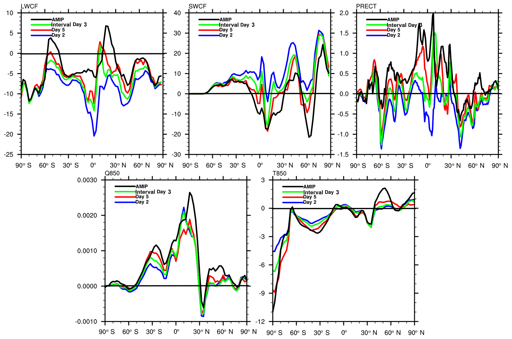
Figure 1The comparison between short-term hindcasts and long-term Atmospheric Model Intercomparison Project (AMIP). The y axis shows bias between the simulations and the observations. The black line is the July mean state from 2000 to 2004 of AMIP simulations. The blue, red, and green lines represent the second day hindcast (labeled as Day 2), the fifth day hindcast (labeled as Day 5), and the Interval Day 3 hindcasts, respectively, for July 2009.
In this study, we use CAM5 as an example. The dynamical core uses the finite-volume method of Lin and Rood (1996) and Lin (2004). Shallow convection is represented as in Park and Bretherton (2009). Deep convection is parameterized by Zhang and McFarlane (1995), which is further modified by Neale et al. (2008) as well as Richter and Rasch (2008). The cloud microphysics is handled by Morrison and Gettelman (2008). Fractional stratiform condensation is calculated by the parameterization of Zhang et al. (2003) and Park et al. (2014). The vertical transport of moisture, momentum, and heat by turbulent eddies is handled by Bretherton and Park (2009). Radiation is calculated by the Rapid Radiative Transfer Model for GCMs (RRTMG; Iacono et al., 2008; Mlawer et al., 1997). Land surface process are represented by the Community Land Model version 4 (CLM4; Lawrence et al., 2011). More details are in Neale et al. (2010).
Two types of model experiments are conducted. One is the short-term hindcast simulations for model tuning. The second is Atmospheric Model Intercomparison Project (AMIP) simulation for verification of the tuned model. The hindcasts are initialized by the Year of Tropical Convection (YOTC) from the European Center for Medium-Range Weather Forecasts (ECMWF) reanalysis. The initialization uses the approach described in Xie et al. (2004) in the Cloud-Associated Parameterizations Testbed (CAPT) developed by the US Department of Energy (US DOE). Since the objective of the tuning approach presented here is not only for auto-calibration of the model, but also for fast calculations, only 1-month hindcasts of July 2009 are used in the tuning process. We carry out the simulations once every 3 days with a 3-day hindcast (labeled as interval Day 3) during the optimization iteration. All of the 3-day simulations for each hindcast run are used to make up the whole monthly data set, which constitutes 31 days of model output. The AMIP simulation is conducted for 2000–2004 by using the observed climatological sea ice and sea surface temperature (Rayner et al., 2003). A simulation of the last 3 years is used for evaluation of the model. All simulations here use 0.9∘ latitude ×1.25∘ longitude horizontal resolution, with 30 vertical layers.
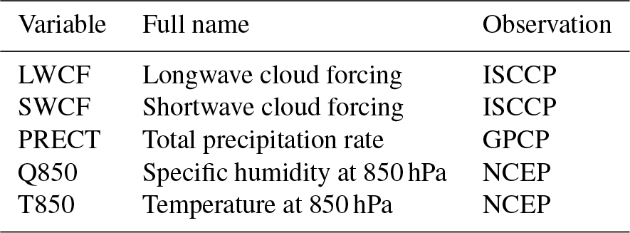
The observational data are from the Global Precipitation Climatology Project (GPCP; Huffman et al., 2001) for precipitation, the International Satellite Cloud Climatology Project (ISCCP) flux data (Trenberth et al., 2009) for radiation fluxes, the CloudSat (Stephens et al., 2002) and the Cloud–Aerosol Lidar and Infrared Pathfinder Satellite Observations (CALIPSO; Winker et al., 2009) for satellite cloud data, and the National Centers for Environmental Prediction/National Center for Atmospheric Research (NCEP/NCAR; Kalnay et al., 1996) reanalysis for humidity and temperature.
For this study, we focus on tuning parameters that are associated with fast physical processes so that short-term hindcasts can be used as an economical way of tuning. The philosophy behind the hindcasts is to keep the model dynamics as close to observation as possible while testing how the model simulates the quantities associated with fast physical processes. In other words, given the correct large-scale atmospheric conditions, errors in the physical variables are used to calibrate the fast physics parameters. This is different from calibration using AMIP simulations in which the circulation responds to the physics. The feasibility of the hindcast approach is based on the fact that errors in atmospheric models show up quickly in initialized experiments (Xie et al., 2004; Klein et al., 2006; Boyle et al., 2008; Hannay et al., 2018; Williams and Brooks, 2008; Martin et al., 2010; Xie et al., 2012; Ma et al., 2013; Ma et al., 2014; Wan et al., 2014). This is also found in the present study. Figure 1 shows the characteristics of the main biases in the CAPT and AMIP simulations in the default model for the five fields of longwave and shortwave cloud forcing (LWCF and SWCF), humidity and temperature at 850 hPa (Q850, T850), and precipitation (PRECT). For CAPT, the biases are for July 2009, while for AMIP they are for July averaged over 3 years. It is seen that the CAPT hindcasts capture a great number of the systematic biases in the AMIP simulations.
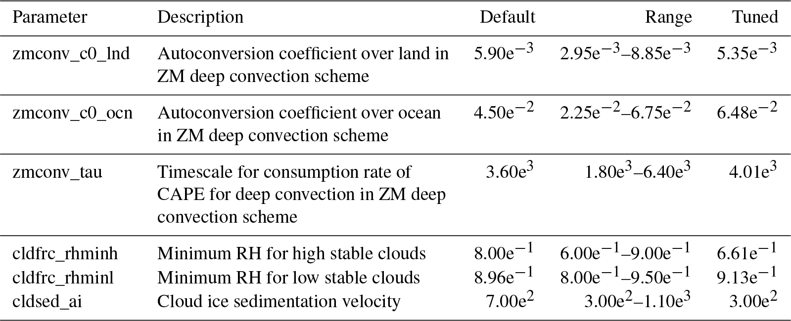
Table 1A summary of parameters to be tuned in CAM5. The default and final tuned optimal values are shown, as well as the valid ranges of the corresponding parameters. ZM indicates the Zhang–McFarlane convection scheme. CAPE indicates convective available potential energy.
Parameter estimation for a complex model involves several choices, including (1) what parameters to optimize and what the range of uncertainties is in the parameters; (2) how to select and construct a performance metric; (3) how to estimate/optimize the parameters in a high-dimensional space; and (4) how to embed the parameter estimation in the process-based evaluation and development of the model. This section describes the first three questions. The last question is left to Sect. 4.
3.1 Model parameters
In our study, the tuning parameters are selected based on the CAM5 sensitivity results of Zhang et al. (2015). They include three parameters from the deep convection scheme and three parameters from the cloud scheme. They are listed in Table 1, along with their default values. The parameters from the convection scheme are the autoconversion efficiency of cloud water to precipitation, separately for land and ocean, and the convective relaxation timescale. The parameters from the cloud scheme are the minimum threshold relative humidity to form clouds, which is an equivalent parameter to the width of the subgrid-scale distribution of relative humidity, separately for high and low clouds, and the sedimentation velocity of ice crystals. All these parameters are known to have large uncertainties.
For the uncertainty ranges of the parameters to be used as bounds of optimal tuning, ideally, they should be derived from the development process of the parameterizations as part of the information from the empirical fitting to observations or to process models. In practice, however, most parameterizations do not contain this information. The uncertainty ranges of the parameters in this study are based on Covey et al. (2013) and previous CAM5 tuning exercises (Yang et al., 2013; Qian et al., 2015). They are listed in Table 1.
Table 2The selected output variables of CAM5 included in the performance metrics and the sources of the corresponding observations.
3.2 The metrics
Several metrics have been used in the literature to quantitatively evaluate and compare the performance of overall simulations of climate models (Gleckler et al., 2008; Murphy et al., 2004; Reichler and Kim, 2008). As a demonstration of the optimization method, in this study we use five fields in Fig. 1 (LWCF, SWCF, PRECT, Q850, and T850) to form a metric. The daily observational data sources for these five fields are listed in Table 2. The tuning metric combines the mean square error (MSE) of the five variables into a single target as the improvement index of model simulation, which is regarded as a function of the uncertain parameter values. When calculating the metric, we first compute the MSE of each target variable of the model simulation against the reanalysis/observations as in Eqs. (1) and (2) for the tuning model and the default model, respectively (Taylor, 2001; Yang et al., 2013; Zhang et al., 2015):
where is the model output at the ith location, and is the corresponding reanalysis or observation data. is the model-simulated variables using the default parameter values. I is the number of grids. w is the weight value based on grid area. The final target improvement index is calculated by using the average of the MSE normalized by that of the control simulation as defined in Eq. (3):
where NF is the number of the variables in Table 2. If the index is less than 1, the tuned simulation is considered as having better performance than the default simulation. The smaller this index value, the better the improvement achieves.
When the differences between model simulation and observation at different grid points are independent of each other and follow normal distributions, minimizing the MSE over all grids would be equivalent to the maximum likelihood estimation of the uncertain parameters. For our experimental design, however, the mismatch between the short-term forecasts and instantaneous observation could be caused by small spatial displacements due to errors in the model initial condition instead of the model parameters. In such cases, errors could be highly correlated between neighboring grids, and the dependence of the metric on the control parameters may be marginalized or obscured. This problem may be lessened in long-term climate simulations, but extra care is needed for short-term forecasts. We therefore choose to use zonally averaged fields from the model and observations in the metric calculation to focus on the effective response at global scale.
3.3 The optimization method
The optimization method is based on an improved downhill simplex optimization algorithm to find a local minimum. Zhang et al. (2015) shows this algorithm can find a good local minimum solution based on the better choice of the initial parameter values. Global optimization algorithms that aim to find the true minimum solution always require an extreme amount of computational cost compared to the method used here, such as the covariance matrix adaptation evolution strategy (Hansen et al., 2003), efficient global optimization (Jones et al., 1998), and genetic algorithm (Holland, 1992), and there is no guarantee they can find one within a limited number of iterations which are often invoked for complicated problems. In practice, Zhang et al. (2015) showed the improved downhill simplex method outperformed the global optimization algorithms with the limited optimal iterations.
The optimization procedure takes two steps. First, preprocessing of selected parameter initial values is carried out to accelerate the convergence of the optimization algorithm and to account for the ill conditioning of the minimization problem. Next, the improved downhill simplex optimization algorithm is utilized to solve the problem due to its fast convergence and low computation for low-dimensional space. Meanwhile, an automatic workflow (Zhang et al., 2015) is used to take care of the complicated configuration process and management of model tuning. In the following, we give a brief description of these two steps. More details can be found in Zhang et al. (2015).
The preprocessing uses a sampling strategy based on the single parameter perturbation (SPP) method, in which, at one time, it perturbs only one parameter with others fixed. The perturbed samples are uniform distribution across parametric space. Equation (3) defines the improvement index for each parameter sample. The distance of samples, defined as the difference between the indexes from using two adjacent samples, is then calculated. We call this step the first-level sampling. If the distance between two adjacent samples is greater than a predefined threshold, more refined samples between these two adjacent samples are conducted. This is the second-level sampling. Finally, the candidate initial values for the optimization method choose the k+1 samples with the best improvement index values, where k is the number of the parameters. In this study, k is 6. The convergence performance of the traditional downhill simplex heavily relies on the quality of its initial values. Inappropriate ones may give rise to ill-conditioned simplex geometry. Therefore, simplex checking is carried out to ensure as many distinct values of parameters as possible during the process of looking for initial values to ensure that the simplex is a well-conditioned geometry.
The downhill simplex algorithm calculates the parameter values and the corresponding improvement index as defined in Eq. (3) in each step of the iterations. The optimal results are achieved by expanding or shrinking the simplex geometry in each optimal step. In the processes of searching for the minimum index, the best set of tuning parameter values up to the current iteration step is kept to look for the direction and magnitude of the increments. The iteration is terminated when the tuning parameters reach quasi-steady state.
Figure 2 summarizes the workflow of the experiments. The workflow is automated. It has two components: model calibration and verification. The calibration uses the hindcasts, the predefined metric, and the optimization algorithm to derive the optimal parameter values. The verification uses the AMIP climate simulation to check how effective the auto-calibration is for the application goal, which is to improve the metric in the AMIP simulation.
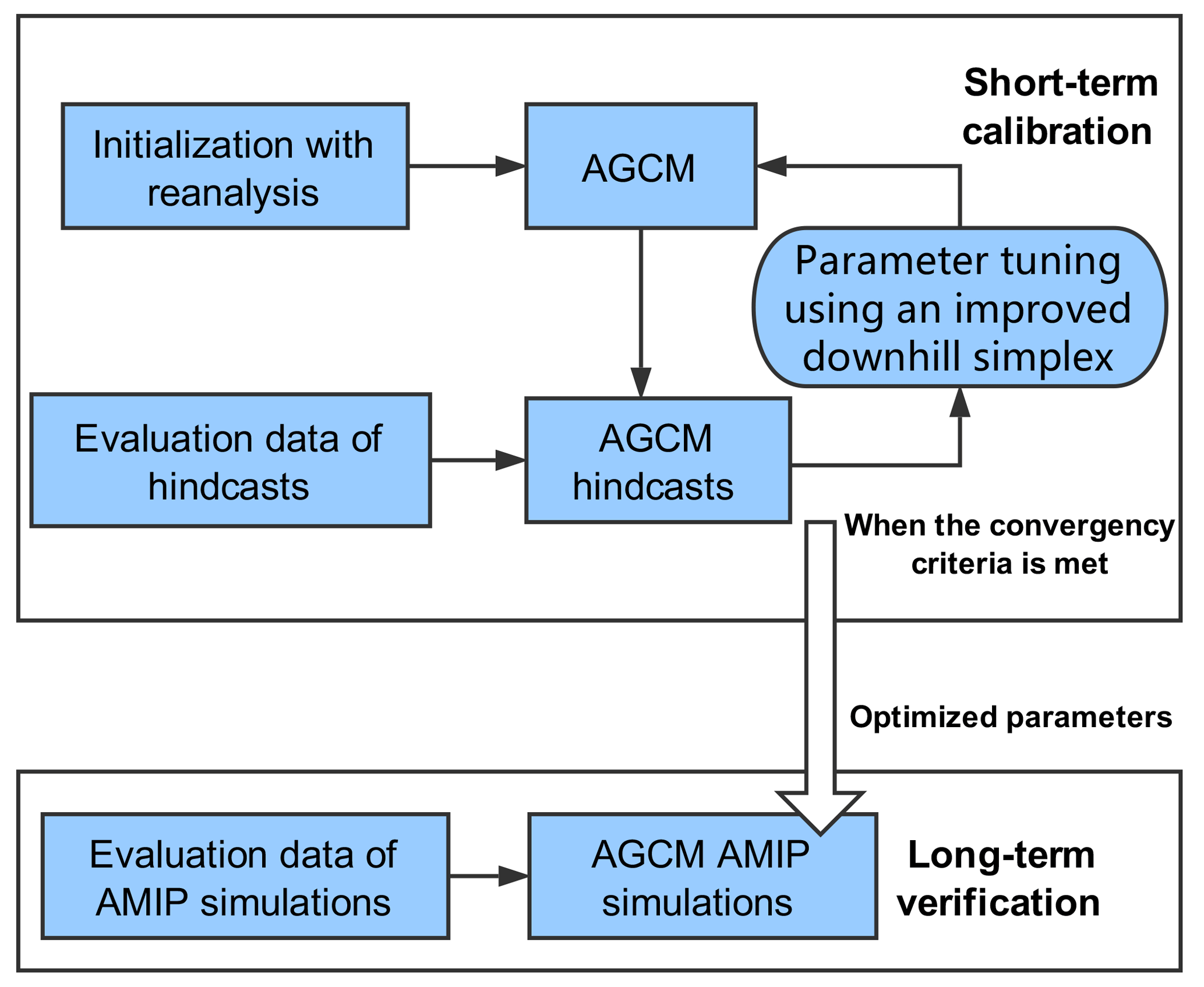
Figure 2Flow diagram of the automatic calibration of parameters via the short-term CAPT and the verification of optimized parameters through long-term AMIP simulations.
4.1 The optimized model
The change of performance index in the optimization iterations as a function of iteration step is shown in Fig. 3. The blue line is the best performance index up to the current step. The red line is the real performance up to the current step. The latter has spikes during the iteration, especially near step 70, suggesting that the performance index in the parameter space has a complex geometry. Each iteration involves 31 days of hindcasts. The iteration is stopped at about the 142nd iteration step when the searched parameters reach quasi-steady state. With 180 computing cores on a Linux cluster, each iteration takes about 50 min. The computational time for an entire optimization is equivalent to about 12 years of an AMIP simulation, which is a tremendous reduction of computing time relative to traditional model tuning.

Figure 3The change of performance index in the optimization iterations. The x axis shows the optimization iterations. The y axis shows the improvement index in Eq. (3). The red line is the index in a given iteration step, while the blue line is the best index up to this time step.
The tuned values of the parameters are given in the column of “tuned” in Table 1. In the default model, the autoconversion parameter c0 is smaller over land than over the oceans, reflecting more aerosols and smaller cloud particle sizes over land than over the oceans. When compared with the default values, the tuned c0 value over land is even smaller, while the value over the ocean is even larger. The parameter that represents the timescale of the convective adjustment is larger in the tuned model than in the default model. For the three parameters in the cloud scheme, the minimum relative humidity in the tuned model is reduced for high clouds but increased for low clouds in the tuned model. The sedimentation velocity of ice crystals is reduced by over a half in the tuned model. The physical justification of these new parameter values is beyond the scope of this paper, but they are all within the range of known uncertainties by design of the optimal tuning. How the parameter change affects the simulation is discussed in Sect. 4.2.
The performance index of the tuned model in the hindcasts and the normalized MSE of the individual fields in the metric are given in Table 3 under the hindcasts column. The performance index is reduced by about 10 % in the tuned model. This is relatively a significant reduction, considering the fact that CAM5 is already a well-tuned model, and a major upgrade of the CAM model from CAM4 to CAM5 also saw that changes in most of the variables are within a 10 % range in terms of RMSE (Flato et al., 2013). Looking at the MSE of the individual fields in the table, we find that the reduction in the performance index is not evenly distributed across the targeted fields. The largest reduction, at about 40 %, is found for the MSE in the LWCF. This is actually not a surprise. Zhang et al. (2015) showed that LWCF is highly sensitive to changes in the convective available potential energy (CAPE) consumption timescale (zmconv_tau) and the minimum relative humidity (RH) for high stable clouds (cldfrc_rhminh). Yang et al. (2013) also indicated the zmconv_tau was sensitive for LWCF. The autoconversion efficiency of cloud water to precipitation (zmconv_c0_lnd and zmconv_c0_ocn) and the cloud ice sedimentation velocity (cldsed_ai) were found to be sensitive for LWCF in Qian et al. (2018). That is to say, all the tuning parameters in this study are very sensitive for LWCF, resulting in this field having the most improvement. There is about 8 % reduction of MSE in PRECT and 4 % reduction in T850. However, two fields, the SWCF and the Q850, are accompanied by 3 % and 1 % increases of errors, respectively. As will be discussed later, this is indication of structural errors in the model whose solution cannot fit to all observations.
Table 3The optimal improvement index of each variable and total comprehensive metric of the CAPT run and AMIP run.
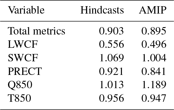
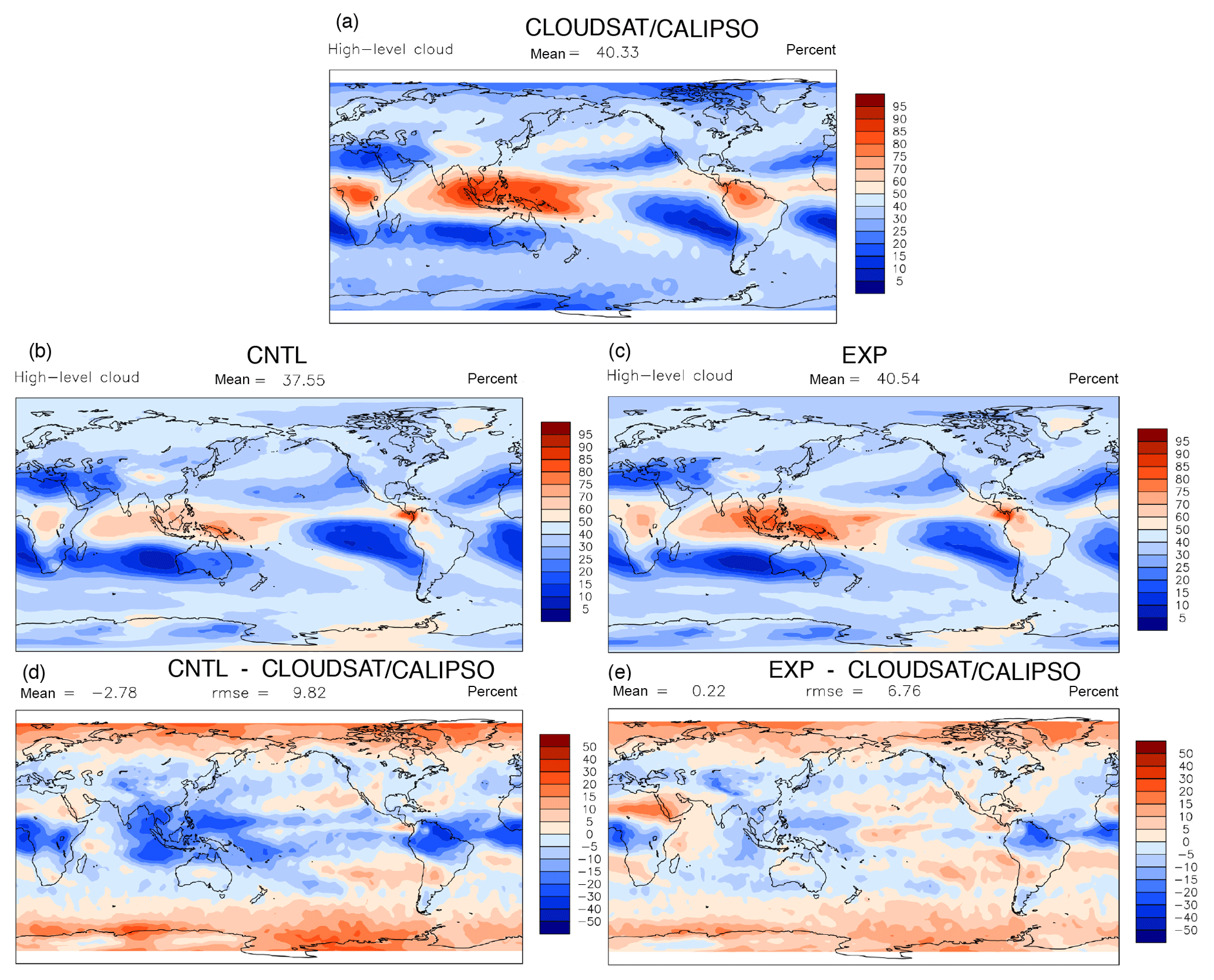
Figure 4The spatial distribution of high cloud amount in the (a) observation, (b) CNTL, (c) EXP, (d) CNTL – observation, and (e) EXP – observation.
The next critical question is whether the optimal results tuned in hindcasts are shown in the AMIP simulation. The last column in Table 3 under the heading of “AMIP” gives the performance index of the tuned model and the normalized MSE of the individual fields from the AMIP simulation. Three things are noted. First, the overall performance index is also improved by about 10 % in the AMIP simulation in the tuned model. Second, as in the hindcasts, the largest improvement is in the LWCF. Third, the fields that were improved in the AMIP simulations are the same as those in the hindcasts. We therefore conclude that the automatic tuning achieved the design goal of the algorithm.
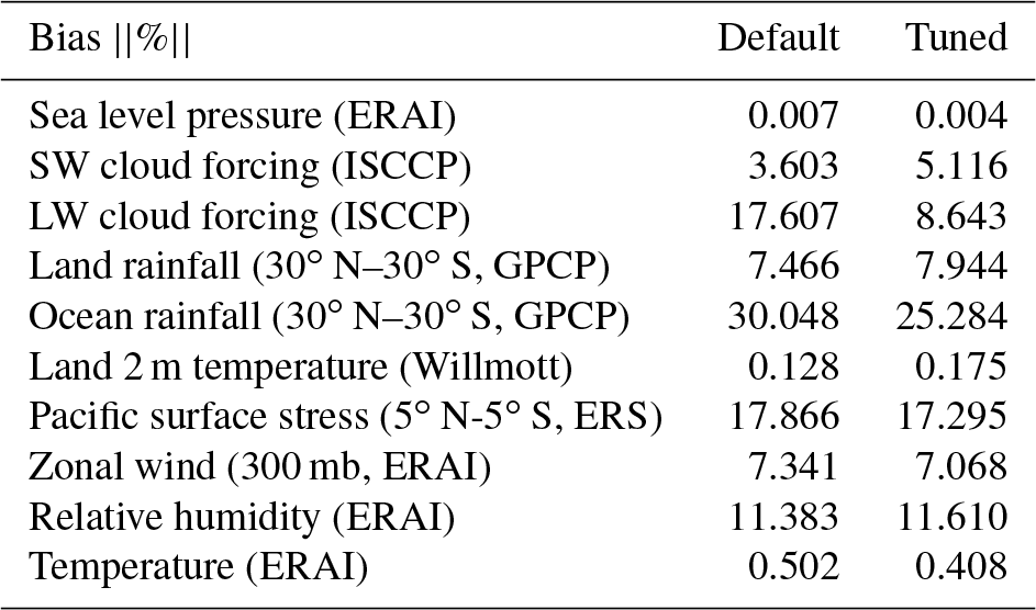
We also examined a 10-variable metric that is used by the Atmospheric Model Working Group (AMWG) of the Community Earth System Model (CESM) (http://www.cesm.ucar.edu/working_groups/Atmosphere/metrics.html, last access: 14 December 2018). The five variables that we used in the performance index are a subset of these fields, except that precipitation in the AMWG metric is separated into land and ocean components. Therefore, there are six additional fields in the AMWG metric. Table 4 shows the percentage bias of the 10 fields between the default/optimized model and the reference observations, which is computed based on two-dimensional monthly mean fields as the follows:
It is seen that among the six new variables, surface pressure, oceanic tropical rainfall, Pacific Ocean surface stress, and zonal wind at 300 hPa are all improved in the tuned model. Increased errors are seen in surface air temperature and precipitation over land. This evaluation is overall consistent with the improved performance metrics shown in Table 3 in which zonally averaged fields were used. This comparison lends credence to the intended objective of the tuning, with the exception over land for which additional parameters may be included for tuning.
Table 4The percentage biases of the 10 fields between the default and tuned models and their reference observations.
4.2 Interpretation of the tuned results
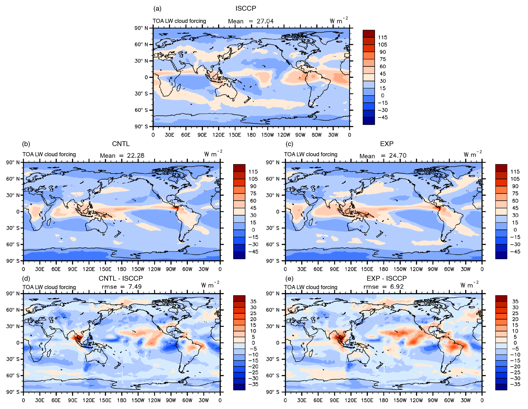
Next, we examine the physical processes behind the changed performance index in the tuned model. Figure 4a, b, and d show, respectively, the annually averaged high cloud amount in the AMIP simulation of the satellite observation from CloudSat and CALIPSO, the default model, and the model bias. It is seen that CAM5 significantly underestimated high clouds in the tropics, including the western Pacific warm pool, and the central Africa and the US, except in the narrow zonal band of the Intertropical Convergence Zone (ITCZ) in the Pacific. The model also underestimated high clouds in regions of middle-latitude storm tracks. Since high clouds have a large impact on the LWCF, these biases in the high clouds would cause underestimation of LWCF. Figure 5a, b, and d show the LWCF in the observation, the default model, and the model bias. The bias field (Fig. 5d) clearly shows that the model significantly underestimates the LWCF. Its spatial pattern largely mirrors the bias field in high cloud amount in Fig. 4d.
In the model optimization, as described before, a smaller relative humidity threshold value for high clouds in the cloud scheme and a smaller sedimentation velocity of ice crystals were derived. These two parameter adjustments can both act to increase high cloud amount and thus longwave cloud forcing. The simulated high cloud and its bias relative to observation are shown in Fig. 4b to e. It can be seen that the overall bias in high cloud is significantly reduced in the tuned model. This leads to reduced negative bias in LWCF in the optimal model (Fig. 5b to e).
Changes in clouds are inevitably accompanied by changes in the SWCF, which was slightly deteriorated in the tuned model as discussed previously. We find that while high clouds are increased in the tuned model, clouds in the middle troposphere are reduced in middle and high latitudes (Fig. 6). This reduction in middle clouds may have compensated the impact of increased high clouds on SWCF, since SWCF is also used in the performance metric. This reduction of middle clouds is consistent with the increased precipitation efficiency parameter c0 in the tuned model over the ocean and the reduced convection to be discussed later.
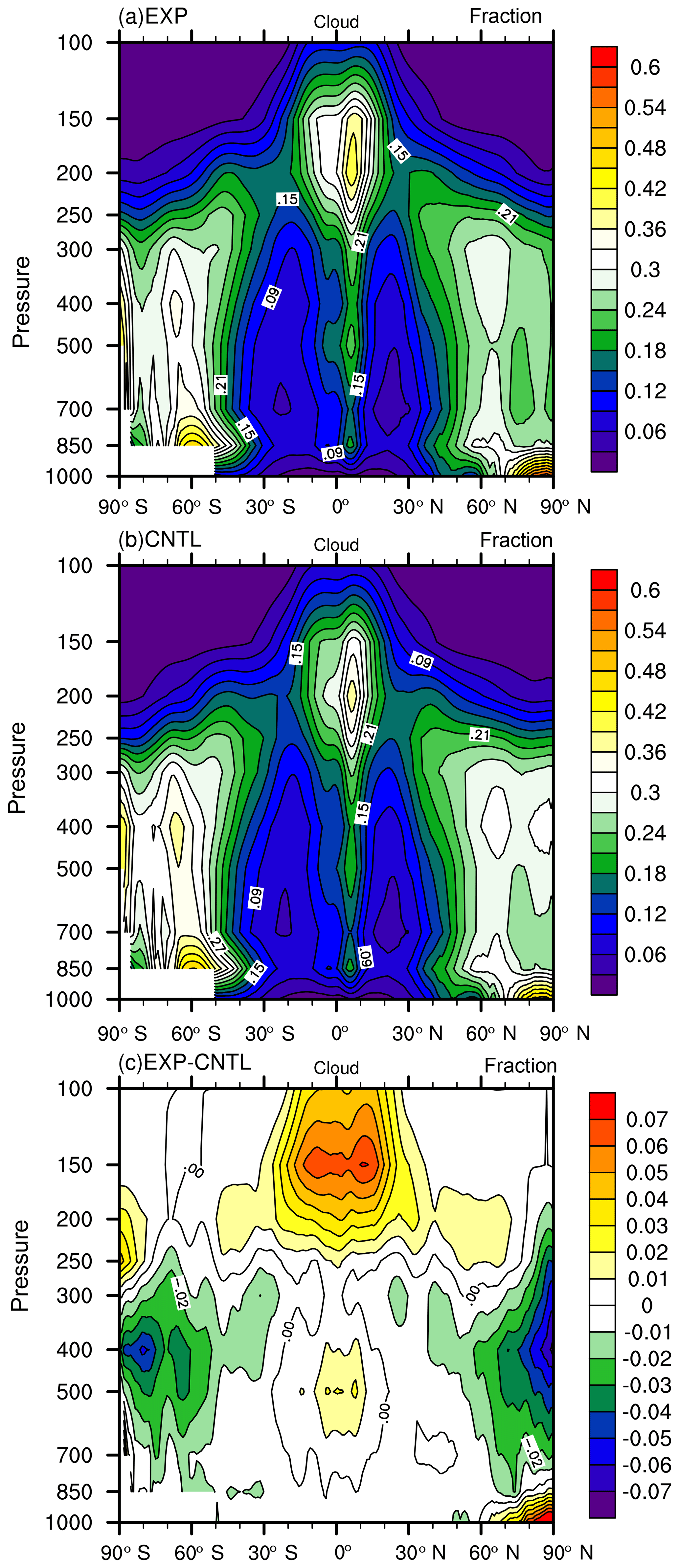
Figure 6Pressure–latitude distributions of cloud fraction in (a) EXP, (b) CNTL, and (c) EXP – CNTL.
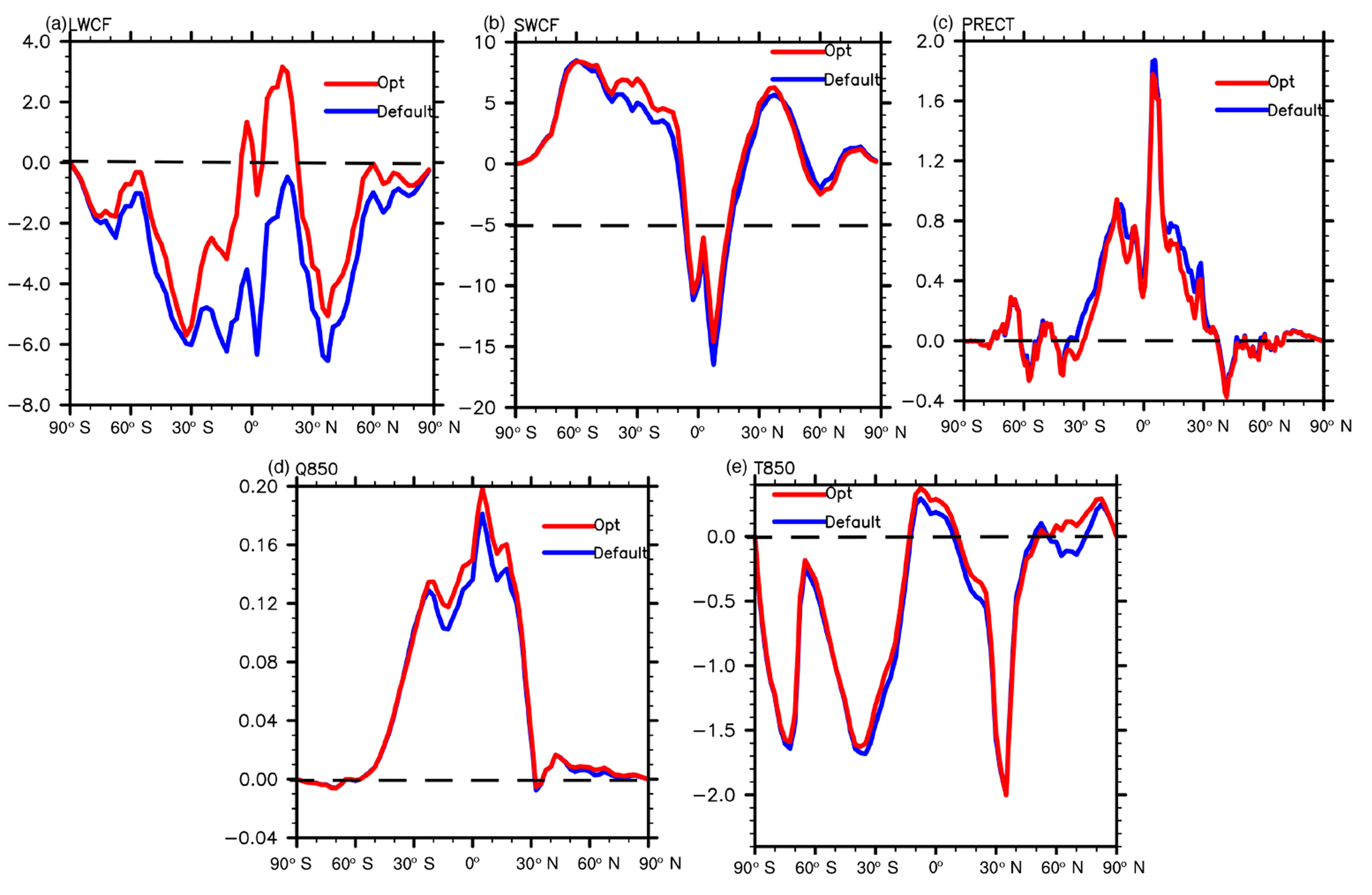
Figure 7Meridional distribution of the AMIP difference between EXP/CNTL and observations of LWCF (a), SWCF (b), PRECT (c), Q850 (d), and T850 (e). The red line is the output variable of EXP. The blue line is the output variable of CNTL.
The impact of the tuning on other targeted fields is less dramatic than on LWCF. To see the impact clearly, we show in Fig. 7 the zonally averaged biases in the AMIP simulation from the default CAM5 as the blue lines and the optimized model as the red lines. The two-dimensional map figures are given in the Supplement. In addition to the large improvement in the LWCF, the overall improvement in PRECT and T850 can be seen. The optimized model simulates slightly smaller precipitation (PRECT) and warmer atmosphere (T850), which are all closer to observations. The reduction in precipitation is consistent with the larger value of the convection adjustment timescale in the tuned model than in the default model. The convection scheme uses a quasi-equilibrium closure based on the CAPE. The adjustment timescale is the denominator in the calculation of the cloud-base convective mass flux. When the timescale is longer, the mass flux is smaller and so is the convective precipitation. This reduction in precipitation is one likely cause of the larger SWCF (less cloud reflection) in the tuned model. In addition to the convection adjustment timescale, other parameters also impact precipitation. In particular, the impact of the increased precipitation efficiency over the ocean in the tuned model should partially offset the impact of the longer convective adjustment timescale. The change of PRECT is the net outcome of the multivariate dependences on all parameters that is found by the automatic optimization algorithm for the overall improvement of the performance index.
The increase in LWCF and the reduced PRECT in the optimal model are energetically consistent for the atmosphere. There is less atmospheric longwave radiative cooling and less condensational heating in the tuned model. The magnitude of the LWCF increase is large (2.42 W m−2) relative to the change in condensational heating (2.03 W m−2) as derived from the change in global mean precipitation amount. As a result, the atmosphere is slightly warmer, which is also closer to observation (Fig. 7e) and this is an improvement to the default model.
While consistent improvements in different fields are desired, this is not always possible. For example, a warmer atmosphere is often accompanied by a moister atmosphere. Since temperature in the tuned model is warmer than that in the default model, there is more moisture in the tuned model. The atmosphere in the default model is already too moist (Fig. 7d). As a result, the performance index in Q850 is slightly deteriorated. Since the optimization is based on a single combined metric of several target variables, the algorithm seeks to minimize this combined metric at the expense of the performance of other variables as long as the total metric is reduced. The fact that the default CAM5 overestimated water vapor and underestimated temperature as shown in Fig. 7d and e indicates structural errors in the model; improving temperature could lead to larger biases in water vapor in the current model.
In summary, the improved performance index in the LWCF is consistent with the dominant impact of the reduced values in the threshold relative humidity for high clouds and the sedimentation velocity of ice crystals. The improvement in PRECT is consistent with the increased convective adjustment timescale. The improvement in T850 is consistent with the large increase in LWCF and reduced radiative cooling of the atmosphere. The deterioration in SWCF is consistent with the impact of increased autoconversion rate, longer convective adjustment timescale, and increased threshold relative humidity of low clouds, all of which can lead to reduction of cloud water. The deterioration in Q850 is likely the result of larger T850 in the tuned model.
These results point to both the benefits and limitation of the described model tuning. The benefit is the improvement in a predefined metric, which has led to improvements in several fields. The limitation is that not all fields can be improved. Some fields may get worse as a result of the algorithm achieving the largest improvement in the total predefined metric. One may use different weights for different fields in Eq. (1) or impose conditional limits on the normalized MSE for the individual fields. The benefits of such alternative approaches will surely depend on specific applications, but structural errors cannot be eliminated by the tuning.
We have presented a method of economic automatic tuning by using short-term hindcasts for 1 month. It is used to optimize CAM5 by adjusting several empirical parameters in its cloud and convection parameterizations. The computational cost of the entire tuning procedure is less than 12 years of a single AMIP simulation. We have demonstrated that the tuning accomplished the design goal of the algorithm. We show about 10 % improvement in our predefined metric for CAM5 that is already a well-calibrated model. Among the five targeted fields of LWCF, SWCF, PRECT, T850, and Q850, the largest improvement is to LWCF, which has about 40 % improvement in the zonal mean MSE. We have shown that while the improvements in LWCF, PRECT, and T850 are consistent with the improved atmospheric energy budget, they lead to slight deterioration in the SWCF and Q850 that reflects structural errors of the model. The overall improvement is also seen in the 10-variable AMWG metrics.
The optimized model contains reduced values of the threshold relative humidity for high clouds and sediment velocity of ice crystals, which act to increase the high cloud amount and increase the longwave cloud forcing, thereby reducing its significant underestimation in the default model. The optimization gave increased convection adjustment time that can explain reduced precipitation in the tuned model and the reduction of the precipitation biases. These two changes also help to reduce the temperature bias. The gains in these fields, however, are accompanied by slight deterioration in shortwave cloud forcing that is consistent with the reduced precipitation, and slight deterioration in humidity that is consistent with the increased temperature. The optimized results can help to understand the interactive effect of multiple parameters and discover the systematic and structural errors by exploring the parameter calibration ultimate performance.
While benefits of the automatic tuning are clearly seen, there are several limitations of using the present workflow for automatic tuning of GCMs. First, not all fields can be simultaneously improved, since parameter tuning cannot eliminate structural errors in the model. Tuning is not an alternative to improving a model, but rather it is an economic way to calibrate some parameters within a candidate parameterization framework. Second, the optimized model may be caused by compensation of errors. Therefore, process-based model evaluation and physical explanation of the model improvements are always necessary. Third, the tuning by using hindcasts is only applicable for parameters affecting fast physics. For model bias that develops over long timescales, such as that from coupled ocean–atmosphere models, this approach cannot be used, although the conceptual approach may be applied with longer integrations. Finally, the choices of the model parameters, uncertainty ranges, and metrics are somewhat subjective. It would be much more satisfactory if their selections could be done automatically and more objectively. Several improvements can be made to the presented method. Different weights can be used for the targeted fields. Sensitivity to different target metrics can be studied. Multiple target metrics may be designed to optimize different sets of parameters. Constraints such as energy balance at the top of the atmosphere may be imposed. It is also possible to use time-varying solutions as metrics to target variabilities such as the Madden–Julian Oscillation (MJO) in models. These could be a subject for future research.
The source code of CAM5 is available from http://www.cesm.ucar.edu/models/cesm1.2/ (NCAR, 2018). The downhill simplex algorithm, the scripts of running the model driven by the optimization algorithm, and the scripts of computing metrics can be found at http://everest.msrc.sunysb.edu/tzhang/capt_tune/GCM_paras_tuner/ (Zhang, 2018a). The observation data which are used to compute the metrics in the short-term hindcast tuning and validate the optimization in AMIP are available at http://everest.msrc.sunysb.edu/tzhang/capt_tune/capt_tune_obs/ (Zhang, 2018b).
The supplement related to this article is available online at: https://doi.org/10.5194/gmd-11-5189-2018-supplement.
TZ, MZ, WX, JH, and WZ designed the tuning framework. MZ and YL evaluated the optimal results. WL, HYM, and SX generated the CAPT data. HYY provided the ISCCP data. MZ, TZ, and XX designed the tuning metrics. TZ, MZ, and WL wrote the paper.
The authors declare that they have no conflict of interest.
This work is partially supported by the National Key R&D Program of China
(grant nos. 2017YFA0604500 and 2016YFA0602100) and the National Natural
Science Foundation of China (grant nos. 91530323 and 41776010). Additional
support is provided by the CMDV project of the CESD of the US Department of
Energy to Stony Brook University. Tao Zhang (partially) and Wuyin Lin are
supported by the CMDV project to BNL. Hsi-Yen Ma and Shaocheng Xie are funded
by the Regional and Global Model Analysis and Atmospheric System Research
Programs of the US Department of Energy, Office of Science, as part of the
Cloud-Associated Parameterizations Testbed. Hsi-Yen Ma and Shaocheng
Xie were supported under the auspices of the US Department of Energy by
the Lawrence Livermore National Laboratory (LLNL) under contract
DE-AC52-07NA27344.
Edited by: Patrick
Jöckel
Reviewed by: two anonymous referees
Allen, M. R., Stott, P. A., Mitchell, J. F., Schnur, R., and Delworth, T. L.: Quantifying the uncertainty in forecasts of anthropogenic climate change, Nature, 407, 617–620, 2000. a
Bardenet, R., Brendel, M., Kégl, B., and Sebag, M.: Collaborative hyperparameter tuning, in: paper presented at the 30th International Conference on Machine Learning (ICML-13), 199–207, ACM, Atlanta, USA, 2013. a
Boyle, J., Klein, S., Zhang, G., Xie, S., and Wei, X.: Climate model forecast experiments for TOGA COARE, Mon. Weather Rev., 136, 808–832, 2008. a
Bretherton, C. S. and Park, S.: A new moist turbulence parameterization in the Community Atmosphere Model, J. Climate, 22, 3422–3448, 2009. a
Covey, C., Lucas, D. D., Tannahill, J., Garaizar, X., and Klein, R.: Efficient screening of climate model sensitivity to a large number of perturbed input parameters, J. Adv. Model. Earth Sy., 5, 598–610, 2013. a
Flato, G., Marotzke, J., Abiodun, B., Braconnot, P., Chou, S. C., Collins, W., Cox, P., Driouech, F., Emori, S., Eyring, V., and Forest, C.: Evaluation of climate models, Climate Change 2013 – The Physical Science Basis: Working Group I Contribution to the Fifth Assessment Report of the Intergovernmental Panel on Climate Change, Cambridge University Press, UK, 741–866, https://doi.org/10.1017/CBO9781107415324.020, 2013 a
Gleckler, P. J., Taylor, K. E., and Doutriaux, C.: Performance metrics for climate models, J. Geophys. Res.-Atmos., 113, D6, https://doi.org/10.1029/2007JD008972, 2008. a
Holland, J. H.: Adaptation in natural and artificial systems: an introductory analysis with applications to biology, control, and artificial intelligence, MIT press, 1992. a
Hack, J. J., Boville, B., Kiehl, J., Rasch, P., and Williamson, D.: Climate statistics from the National Center for Atmospheric Research community climate model CCM2, J. Geophys. Res.-Atmos., 99, 20785–20813, 1994. a
Hakkarainen, J., Ilin, A., Solonen, A., Laine, M., Haario, H., Tamminen, J., Oja, E., and Järvinen, H.: On closure parameter estimation in chaotic systems, Nonlinear Proc. Geoph., 19, 127–143, 2012. a
Hannay, C., Williamson, D., Olson, J., Neale, R., Gettelman, A., Morrison, H., Park, S., and Bretherton, C.: Short Term forecasts along the GCSS Pacific Cross-section: Evaluating new Parameterizations in the Community Atmospheric Model, available at: http://www.cgd.ucar.edu/cms/hannay/publications/GCSS2008.pdf, last access: 14 December 2018. a
Hansen, N., Müller, S. D., and Koumoutsakos, P.: Reducing the time complexity of the derandomized evolution strategy with covariance matrix adaptation (CMA-ES), Evol. Comput., 11, 1–18, 2003. a
Huffman, G. J., Adler, R. F., Morrissey, M. M., Bolvin, D. T., Curtis, S., Joyce, R., McGavock, B., and Susskind, J.: Global precipitation at one-degree daily resolution from multisatellite observations, J. Hydrometeorol., 2, 36–50, https://doi.org/10.1175/1525-7541(2001)002<0036:GPAODD>2.0.CO;2, 2001. a
Iacono, M. J., Delamere, J. S., Mlawer, E. J., Shephard, M. W., Clough, S. A., and Collins, W. D.: Radiative forcing by long-lived greenhouse gases: Calculations with the AER radiative transfer models, J. Geophys. Res.-Atmos., 113, D13, https://doi.org/10.1029/2008JD009944, 2008. a
Jones, D. R., Schonlau, M., and Welch, W. J.: Efficient global optimization of expensive black-box functions, J. Global Optim., 13, 455–492, 1998. a
Kalnay, E., Kanamitsu, M., Kistler, R., Collins, W., Deaven, D., Gandin, L., Iredell, M., Saha, S., White, G., Woollen, J., and Zhu, Y.: The NCEP/NCAR 40-year reanalysis project, B. Am. Meteorol. Soc., 77, 437–471, https://doi.org/10.1175/1520-0477(1996)077<0437:TNYRP>2.0.CO;2, 1996. a
Klein, S. A., Jiang, X., Boyle, J., Malyshev, S., and Xie, S.: Diagnosis of the summertime warm and dry bias over the US Southern Great Plains in the GFDL climate model using a weather forecasting approach, Geophys. Res. Lett., 33, 18, https://doi.org/10.1029/2006GL027567, 2006. a
Lawrence, D. M., Oleson, K. W., Flanner, M. G., Thornton, P. E., Swenson, S. C., Lawrence, P. J., Zeng, X., Yang, Z. L., Levis, S., Sakaguchi, K., and Bonan, G. B.: Parameterization improvements and functional and structural advances in version 4 of the Community Land Model, J. Adv. Model. Earth Sy., 3, 1, https://doi.org/10.1029/2011MS00045, 2011. a
Li, L., Wang, B., Dong, L., Liu, L., Shen, S., Hu, N., Sun, W., Wang, Y., Huang, W., Shi, X., Pu, Y., and Yang, G.: Evaluation of grid-point atmospheric model of IAP LASG version 2 (GAMIL2), Adv. Atmos. Sci., 30, 855–867, 2013. a
Lin, S.-J.: A “vertically Lagrangian” finite-volume dynamical core for global models, Mon. Weather Rev., 132, 2293–2307, 2004. a
Lin, S.-J. and Rood, R. B.: Multidimensional flux-form semi-Lagrangian transport schemes, Mon. Weather Rev., 124, 2046–2070, 1996. a
Ma, H.-Y., Xie, S., Boyle, J., Klein, S., and Zhang, Y.: Metrics and diagnostics for precipitation-related processes in climate model short-range hindcasts, J. Climate, 26, 1516–1534, 2013. a
Ma, H. Y., Xie, S., Klein, S. A., Williams, K. D., Boyle, J. S., Bony, S., Douville, H., Fermepin, S., Medeiros, B., Tyteca, S., and Watanabe, M.: On the correspondence between mean forecast errors and climate errors in CMIP5 models, J. Climate, 27, 1781–1798, 2014. a
Martin, G., Milton, S., Senior, C., Brooks, M., Ineson, S., Reichler, T., and Kim, J.: Analysis and reduction of systematic errors through a seamless approach to modeling weather and climate, J. Climate, 23, 5933–5957, 2010. a
Mlawer, E. J., Taubman, S. J., Brown, P. D., Iacono, M. J., and Clough, S. A.: Radiative transfer for inhomogeneous atmospheres: RRTM, a validated correlated-k model for the longwave, J. Geophys. Res.-Atmos., 102, 16663–16682, 1997. a
Morrison, H. and Gettelman, A.: A new two-moment bulk stratiform cloud microphysics scheme in the Community Atmosphere Model, version 3 (CAM3). Part I: Description and numerical tests, J. Climate, 21, 3642–3659, 2008. a
Murphy, J. M., Sexton, D. M., Barnett, D. N., Jones, G. S., Webb, M. J., Collins, M., and Stainforth, D. A.: Quantification of modelling uncertainties in a large ensemble of climate change simulations, Nature, 430, 768–772, 2004. a
NCAR: CESM1.2 SERIES PUBLIC RELEASE, available at: http://www.cesm.ucar.edu/models/cesm1.2/, last access: 14 December 2018. a
Neale, R. B., Richter, J. H., and Jochum, M.: The impact of convection on ENSO: From a delayed oscillator to a series of events, J. Climate, 21, 5904–5924, 2008. a
Neale, R. B., Chen, C. C., Gettelman, A., Lauritzen, P. H., Park, S., Williamson, D. L., Conley, A. J., Garcia, R., Kinnison, D., Lamarque, J. F., and Marsh, D.: Description of the NCAR community atmosphere model (CAM 5.0), NCAR Tech. Note NCAR/TN-486+ STR, 2010. a, b
Neelin, J. D., Bracco, A., Luo, H., McWilliams, J. C., and Meyerson, J. E.: Considerations for parameter optimization and sensitivity in climate models, P. Natl. Acad. Sci. USA, 107, 21349–21354, 2010. a
Park, S. and Bretherton, C. S.: The University of Washington shallow convection and moist turbulence schemes and their impact on climate simulations with the Community Atmosphere Model, J. Climate, 22, 3449–3469, 2009. a
Park, S., Bretherton, C. S., and Rasch, P. J.: Integrating cloud processes in the Community Atmosphere Model, version 5, J. Climate, 27, 6821–6856, 2014. a
Qian, Y., Yan, H., Hou, Z., Johannesson, G., Klein, S., Lucas, D., Neale, R., Rasch, P., Swiler, L., Tannahill, J., and Wang, H.: Parametric sensitivity analysis of precipitation at global and local scales in the Community Atmosphere Model CAM5, J. Adv. Model. Earth Sy., 7, 382–411, 2015. a, b, c, d
Qian, Y., Wan, H., Rasch, P., Zhang, K., Ma, P.-L., Lin, W., Xie, S., Singh, B., Larson, V., Neale, R., Gettelman, A., Bogenschutz, P., Wang, H., and Zhao, C.: Parametric sensitivity in ACME-V1 atmosphere model revealed by short Perturbed Parameters Ensemble (PPE) simulations, available at: https://climatemodeling.science.energy.gov/sites/default/files/presentations/Qian-ShortSimulation-2016SpringMeeting-ACME_Poster.pdf, last access: 12 January 2018. a
Rayner, N., Parker, D. E., Horton, E., Folland, C., Alexander, L., Rowell, D., Kent, E., and Kaplan, A.: Global analyses of sea surface temperature, sea ice, and night marine air temperature since the late nineteenth century, J. Geophys. Res.-Atmos., 108, 1871–2000, 2003. a
Reichler, T. and Kim, J.: How well do coupled models simulate today's climate?, B. Am. Meteorol. Soc., 89, 303–311, 2008. a
Richter, J. H. and Rasch, P. J.: Effects of convective momentum transport on the atmospheric circulation in the Community Atmosphere Model, version 3, J. Climate, 21, 1487–1499, 2008. a
Stephens, G. L., Vane, D. G., Boain, R. J., Mace, G. G., Sassen, K., Wang, Z., Illingworth, A. J., O'connor, E. J., Rossow, W. B., Durden, S. L., and Miller, S. D.: The CloudSat mission and the A-Train: A new dimension of space-based observations of clouds and precipitation, B. Am. Meteorol. Soc., 83, 1771–1790, https://doi.org/10.1175/BAMS-83-12-1771, 2002. a
Taylor, K. E.: Summarizing multiple aspects of model performance in a single diagram, J. Geophys. Res.-Atmos., 106, 7183–7192, 2001. a
Trenberth, K. E., Fasullo, J. T., and Kiehl, J.: Earth's global energy budget, B. Am. Meteorol. Soc., 90, 311–323, https://doi.org/10.1175/2008BAMS2634.1, 2009. a
Wan, H., Rasch, P. J., Zhang, K., Qian, Y., Yan, H., and Zhao, C.: Short ensembles: an efficient method for discerning climate-relevant sensitivities in atmospheric general circulation models, Geosci. Model Dev., 7, 1961–1977, https://doi.org/10.5194/gmd-7-1961-2014, 2014. a, b
Wang, C., Duan, Q., Gong, W., Ye, A., Di, Z., and Miao, C.: An evaluation of adaptive surrogate modeling based optimization with two benchmark problems, Environ. Modell. Softw., 60, 167–179, 2014. a
Wang, G. G. and Shan, S.: Review of metamodeling techniques in support of engineering design optimization, J. Mech. Design., 129, 370–380, 2007. a
Williams, K. and Brooks, M.: Initial tendencies of cloud regimes in the Met Office Unified Model, J. Climate, 21, 833–840, 2008. a
Williams, P. D.: Modelling climate change: the role of unresolved processes, Philos. T. Roy. Soc. A, 363, 2931–2946, 2005. a
Winker, D. M., Vaughan, M. A., Omar, A., Hu, Y., Powell, K. A., Liu, Z., Hunt, W. H., and Young, S. A.: Overview of the CALIPSO mission and CALIOP data processing algorithms, J. Atmos. Ocean. Tech., 26, 2310–2323, https://doi.org/10.1175/2009JTECHA1281.1, 2009. a
Xie, S., Zhang, M., Boyle, J. S., Cederwall, R. T., Potter, G. L., and Lin, W.: Impact of a revised convective triggering mechanism on Community Atmosphere Model, version 2, simulations: Results from short-range weather forecasts, J. Geophys. Res.-Atmos., 109, D14, https://doi.org/10.1029/2004JD004692, 2004. a, b
Xie, S., Ma, H.-Y., Boyle, J. S., Klein, S. A., and Zhang, Y.: On the correspondence between short-and long-time-scale systematic errors in CAM4/CAM5 for the year of tropical convection, J. Climate, 25, 7937–7955, 2012. a
Yang, B., Qian, Y., Lin, G., Leung, L. R., Rasch, P. J., Zhang, G. J., McFarlane, S. A., Zhao, C., Zhang, Y., Wang, H., Wang, M., and Liu, X.: Uncertainty quantification and parameter tuning in the CAM5 Zhang-McFarlane convection scheme and impact of improved convection on the global circulation and climate, J. Geophys. Res.-Atmos., 118, 395–415, 2013. a, b, c, d, e, f
Zhang, G. J. and McFarlane, N. A.: Sensitivity of climate simulations to the parameterization of cumulus convection in the Canadian Climate Centre general circulation model, Atmos. Ocean, 33, 407–446, 1995. a
Zhang, M., Lin, W., Bretherton, C. S., Hack, J. J., and Rasch, P. J.: A modified formulation of fractional stratiform condensation rate in the NCAR Community Atmospheric Model (CAM2), J. Geophys. Res.-Atmos., 108, ACL–10, https://doi.org/10.1029/2002JD002523, 2003. a
Zhang, T., Li, L., Lin, Y., Xue, W., Xie, F., Xu, H., and Huang, X.: An automatic and effective parameter optimization method for model tuning, Geosci. Model Dev., 8, 3579–3591, https://doi.org/10.5194/gmd-8-3579-2015, 2015. a, b, c, d, e, f, g, h, i
Zhang, T., Xie, F., Xue, W., Li, L.-J., Xu, H.-Y., and Wang, B.: Quantification and optimization of parameter uncertainty in the grid-point atmospheric model GAMIL2, Chinese J. Geophys.-CH., 59, 465–475, 2016. a
Zhang, T.: Codes of parameter optimization method via CAPT, available at: http://everest.msrc.sunysb.edu/tzhang/capt_tune/GCM_paras_tuner/, last access: 14 December 2018a. a
Zhang, T.: Metrics observation data of parameter optimization method via CAPT, available at: http://everest.msrc.sunysb.edu/tzhang/capt_tune/capt_tune_obs/, last access: 14 December 2018b. a
Zhao, C., Liu, X., Qian, Y., Yoon, J., Hou, Z., Lin, G., McFarlane, S., Wang, H., Yang, B., Ma, P.-L., Yan, H., and Bao, J.: A sensitivity study of radiative fluxes at the top of atmosphere to cloud-microphysics and aerosol parameters in the community atmosphere model CAM5, Atmos. Chem. Phys., 13, 10969–10987, https://doi.org/10.5194/acp-13-10969-2013, 2013. a, b