the Creative Commons Attribution 4.0 License.
the Creative Commons Attribution 4.0 License.
 | 08 Feb 2018
BEATBOX v1.0: Background Error Analysis Testbed with Box Models
Christoph Knote
Jérôme Barré
Max Eckl
The Background Error Analysis Testbed (BEATBOX) is a new data assimilation framework for box models. Based on the BOX Model eXtension (BOXMOX) to the Kinetic Pre-Processor (KPP), this framework allows users to conduct performance evaluations of data assimilation experiments, sensitivity analyses, and detailed chemical scheme diagnostics from an observation simulation system experiment (OSSE) point of view. The BEATBOX framework incorporates an observation simulator and a data assimilation system with the possibility of choosing ensemble, adjoint, or combined sensitivities. A user-friendly, Python-based interface allows for the tuning of many parameters for atmospheric chemistry and data assimilation research as well as for educational purposes, for example observation error, model covariances, ensemble size, perturbation distribution in the initial conditions, and so on. In this work, the testbed is described and two case studies are presented to illustrate the design of a typical OSSE experiment, data assimilation experiments, a sensitivity analysis, and a method for diagnosing model errors. BEATBOX is released as an open source tool for the atmospheric chemistry and data assimilation communities.


Current regional and global models of the composition of Earth's atmosphere exhibit a high level of complexity due to the combination of chemical and meteorological processes such as transport, thermodynamics, radiation, or precipitation. But “just” gas-phase chemistry itself already has a considerable amount of complexity. The number of variables (chemical compounds) and equations (chemical reactions) in current model representations of tropospheric chemistry (“mechanisms”) can vary by 2 orders of magnitude (from 102 to 104). Compare, for example, two well-known mechanisms: the Model for Ozone And Related Chemical Tracers version T1 (MOZART-T1; Emmons et al., 2010; Knote et al., 2014) uses 134 species and 250 reactions, whereas the Master Chemical Mechanism version 3.3 (MCMv3.3; Jenkin et al., 2015) employs over 5000 species and over 15 000 reactions. MCMv3.3 is called a “near-explicit” chemical mechanism, which describes in detail the gas-phase chemical processes involved in the tropospheric degradation of volatile organic compounds (VOCs). On the other hand, MOZART-T1 uses a simplified (“lumped”) representation of VOCs. This reduction in complexity is advantageous as it reduces the computational demand, but can lead to significant errors in the prediction of atmospheric composition. The choice of a chemical mechanism is therefore a trade-off: while MCMv3.3 would be desirable due to its fidelity in representing atmospheric chemistry, it cannot currently be used in large-scale 3-D atmospheric simulation due to its computational demand. MOZART-T1 is less accurate, but also much more economic.
Investigating the performance of chemical mechanisms is often done using zero-dimensional (0-D) box models. Numerous studies have used box models to study reactive gas-phase chemistry and provide intercomparisons and validation of mechanisms. Emmerson et al. (2009) provided a comprehensive comparison of the MCM mechanism with six tropospheric chemistry lumped schemes that could be used within chemistry transport models. Archibald et al. (2010) performed an intercomparison of the gas-phase mechanism for isoprene degradation in a box model with various mechanisms widely used in 3-D models. More recently, Coates et al. (2015) compared MCM to simplified VOC mechanisms to look at ozone production for a selection of VOCs representative of urban air masses. Knote et al. (2015) conducted box model simulations using different chemical mechanisms and compared them to each other to understand mechanism-specific biases during a 3-D model intercomparison. Mazzuca et al. (2016) used an observation-constrained box model with a lumped carbon-bond mechanism to study photochemical oxidation and ozone production processes along a research aircraft campaign. Wolfe et al. (2016) presented a tool for 0-D atmospheric modeling that can use different chemical mechanisms and methods of photolysis frequency calculations.
This non-exhaustive list of recent studies using box models to study tropospheric chemistry shows the importance of and need for such tools. Box models are attractive due to their simplicity and low computational cost, but cannot provide a realistic representation of the entire atmosphere because they lack vertical and horizontal diffusion, boundary conditions, and numerous other processes that 3-D models take into account. In that regard, box model studies should not focus on replicating the most accurate predictions but rather aim at gaining significant fundamental and conceptual understanding of a given system of ordinary differential equations (ODEs), in the present case the one that governs tropospheric chemistry.
Another aspect of box models or reduced complexity models is the applicability to data assimilation research. Low dimension and/or box models are often used to design new data assimilation algorithms and to conceptually prove the advantage of a given method. In data assimilation theory, the use of the Lorenz model and other simple systems is common practice: Sandu et al. (2005) used a box model approach to design an adjoint-based sensitivity analysis for reactive gas-phase tropospheric chemistry. Ott et al. (2004) used a Lorenz-96 model to introduce a new formulation of the ensemble Kalman filter approach. Van Leeuwen (2010) also used the Lorenz model to investigate nonlinear advanced data assimilation techniques such as the particle filter.
Atmospheric composition data assimilation, and more generally inversion, is complex and computationally demanding. Reactive gas-phase photochemistry is highly nonlinear and has to deal with hundreds to thousands of variables. There is a need for a tool that allows for the exploration of suitable novel data assimilation approaches for atmospheric chemistry, assesses uncertainty and errors of a given chemical mechanism, and performs chemical sensitivity analysis from one parameter to another. All this should be possible with minimal computational expenses and coding skills required. In this paper, we present a new framework based on BOXMOX (BOX MOdel eXtension to KPP; Knote et al., 2015) called BEATBOX (Background Error Analysis Testbed with Box Models) that is able to cycle data assimilation windows, calculate adjoint, ensemble, or even more advanced sensitivity analysis, and assess box model errors and uncertainties. In Sect. 2 we present in detail the structure of BEATBOX and its algorithms, as exemplified through case studies that we discuss in Sect. 3.
The Background Error Analysis Testbed with Box Models (BEATBOX) is a suite of tools that allows for a simple and fast investigation, comparison, and evaluation of any system of ordinary differential equations (ODEs) evolving over time. By “background error” we designate a general term for model error characterization. In this study, BEATBOX is used within the scope of atmospheric chemical mechanisms. Currently, the BEATBOX framework consists of a forecasting tool, the BOX MOdel eXtension (BOXMOX; Knote et al., 2015) to the Kinetic Pre-Processor (KPP; Sandu and Sander, 2006), presented in Sect. 2.1, and a data assimilation tool, which will be introduced in Sect. 2.2.
The BEATBOX structure is built upon observing system simulation experiments (OSSEs; Arnold and Dey, 1986). OSSEs are generally used in the field of numerical weather prediction (e.g., Kuo et al., 1998; Wang et al., 2008; Liu et al., 2009) and atmospheric composition and air quality predictions (e.g., Edwards et al., 2009; Claeyman et al., 2011; Barré et al., 2015, 2016). OSSEs allow for an assessment of the benefit of a potential new type of instrument for environmental predictions using a data assimilation system and are of crucial importance to define the requirements of a given instrument. Space agencies such as the National Aeronautics and Space Agency (NASA) and the European Space Agency (ESA) hence support OSSEs as tools to verify scientific readiness levels for proposed space missions. Also, the model and data assimilation requirements should be assessed to meet a required predictive capability. The current BEATBOX framework employs a box modeling approach to avoid the space dimension problem – the dimensionality of the problem is reduced to time and variables only. Hence the geometry, radiative specifications, and spatial resolution of a new instrument type are irrelevant. What can be easily explored within BEATBOX is the type of data assimilation method used (e.g., background error covariance calculations, localizations, inflation methods), the revisit time (or temporal sampling) of a measurement, the variable(s) observed, and straightforward comparisons between sets of ODEs (chemical schemes in our case).
A number of issues regarding the OSSE technique should be mentioned as well. Performing an OSSE could be costly in terms of setup, design, and computation. Numerical integration of the most state-of-the-art representation of the Earth system for sampling observations and benchmarking could be intensively costly and requires highly skilled staff and extensive collaboration between research entities. Approximations are often required to make experiments possible (e.g., the “identical twin” problem), necessitating careful diagnosis of the results that could limit scientific conclusions.
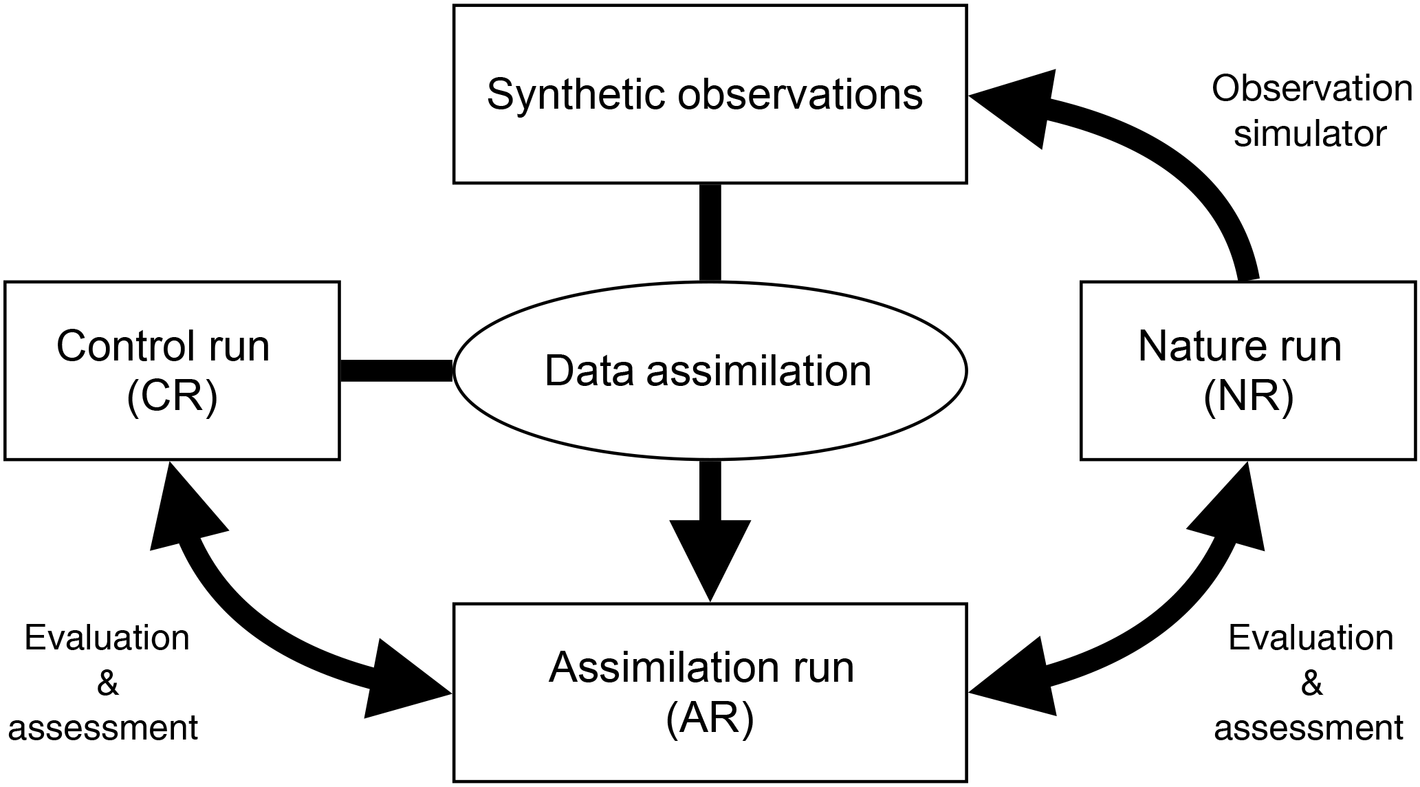
Ultimately an OSSE should be used to highlight model deficiencies and inaccuracies, and provide direct guidance for model improvement. In that context, BEATBOX could be considered as a derived OSSE framework focused on data assimilation techniques and model improvement rather than the benefit of new or future types of observations. Starting from a scientific question or hypothesis to be validated (or rejected) that fits the topics mentioned above, several components are required (Fig. 1):
-
a nature run (NR) considered as the “true state” (the NR supposes to use the best model representation possible considering the state of the art; in this study, we used the Master Chemical Mechanism (MCMv3.3.1) as the NR);
-
a control run (CR) as the prior estimated state of the atmosphere (compared to the NR, a simplified or degraded model should be used, for example a set of ODEs that can be implemented in large-scale 3-D models; in this study, we use MOZART-T1);
-
an observation simulator that generates synthetic observation by sampling the NR (observation errors also need to be simulated);
-
an assimilation run (AR) that is produced using the data assimilation tool merging the synthetic observation with the CR to produce the best estimate possible of the state; and
-
a suite of diagnostic tools that use NR, CR, and AR designed to point out model and data assimilation technique limitations, ultimately providing a direct feedback for model improvement.
The BEATBOX framework has the capability to loop over several assimilation cycles, also called “cycling”. Cycling with BEATBOX is schematically displayed in Fig. 2. Every cycle starts with the forecast step. By applying their respective model, the NR, the forecast (F), and the CR are processed from cycle t−1 to cycle t. Then, NRt is used to generate synthetic observations through the observation operator H (see Sect. 2.2.2). These observations are assimilated into the forecast to produce the analysis with j as the data assimilation method of choice using a gain Kj (see Sects. 2.2.3–2.2.5). Then, will be used to generate new initial conditions IC to start a new forecast. CRt serves as a reference to determine the performance of the assimilation method j after t forecast cycles. The forecast can be taken to quantify the skill of the assimilation method j at the current cycle t. Afterwards, the cycle t+1 starts with its forecast step.
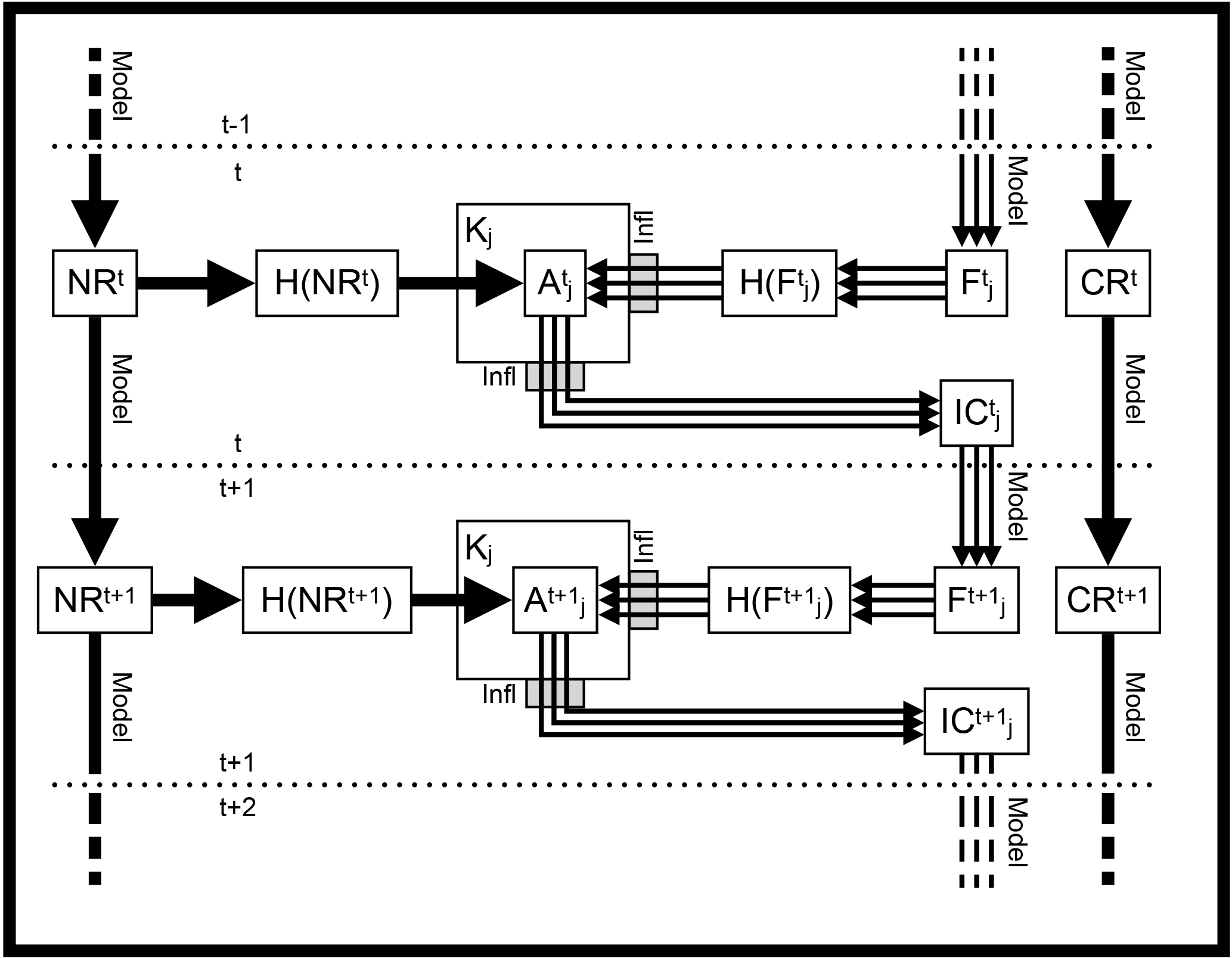
Figure 2The cycling sequence with BEATBOX, with the assimilation window t, the assimilation method j, control run CR, nature run NR, observation operator H, gain K, analysis A, initial condition IC, and forecast F.
2.1 Forecasting tool
2.1.1 The box model BOXMOX
BOXMOX performs box model simulations with different chemical mechanisms
using varying sets of input parameters. BOXMOX relies on KPP, a code
generator that simplifies the numerical integration of systems of ODEs. The
temporal evolution of concentrations of chemical compounds due to
photochemistry is a prime example of such a system. KPP takes a predefined
set of chemical equations (in our case a chemical mechanism) written in a
symbolic, human-readable language and generates a computer code (FORTRAN,
Matlab, C) containing a numerical solver to integrate the system over time. A
number of integration methods are available (e.g., Rosenbrock or Runge–Kutta
methods). In addition to predicting the evolution of concentrations over
time, the resulting solver also delivers the Jacobian and Hessian
matrices of the system. Adjoint models can be generated and tuned (Sandu et
al., 2003) and the Jacobians of the adjoint of the model can be obtained (see
Sect. 2.2.3). Building upon KPP, BOXMOX provides additional processes
typically used in box model studies (emissions, photolysis, deposition,
mixing) and allows for convenient data input. BOXMOX makes simulations of
chamber experiments, Lagrangian-type air parcel studies, and a description of
the chemistry in the atmospheric boundary layer feasible without effort.
Input is done via simple text files: initial conditions, photolysis rates,
temperature, boundary layer height, detrainment and entrainment, turbulent mixing,
emission, and deposition are possible input parameters. BOXMOX is a
stand-alone C and Fortran program running on Linux or Mac OS X. In this work we
have extended BOXMOX with an interface written in the Python language
(boxmox package) to interface more easily with BEATBOX.
BEATBOX uses BOXMOX to rapidly generate a large number of simulations with perturbed input parameters. The temperature, (time-varying) photolysis rates, and initial concentrations of each species included in the investigated chemical mechanism can be perturbed independently. Ensemble members can be generated by producing normal- or lognormal-distributed perturbation factors with the possibility to adjust the mean and the standard deviation for each perturbed variable. These perturbation factors are then multiplied by the relevant initial values to produce an ensemble of initial conditions.
In this work, we demonstrate the BEATBOX capabilities using MCMv3.3.1 as NR. Because of its near-explicit representation of atmospheric chemistry, MCMv3.3.1 is a good choice to be seen as the assumed “truth” within the context of an OSSE. The MOZART-T1 chemical mechanism is employed as the simplified and/or degraded model (CR, AR).
2.1.2 Input data generation
BOXMOX comes with a tool to generate input data from field campaign
observations (the genbox Python package). Translation to mechanism-specific
species naming and lumping is achieved using a translation tool (the
chemspectranslator package) originally based on the emission database created
by Bill Carter (UC Riverside; http://www.cert.ucr.edu/~carter/emitdb).
The current system uses data collected in the FRAPPE (Front Range Air
Pollution and Photochemistry Experiment) field campaign (frappedata package).
During FRAPPE, a number of flight measurements with remote sensing and
in situ devices of numerous quantities were performed, including
concentrations of chemical species, photolysis rates, and temperature. In the
examples shown we use measurements taken during FRAPPE with the NCAR C130
research aircraft to initialize the box model. Photolysis rates
measured during FRAPPE are used in the examples shown here. For other
cases in which photolysis rates are missing, we provide the ability to use
photolysis rates calculated by the Tropospheric Ultraviolet Visible (TUV)
radiation model version 5.1 (Madronich and Flocke, 1997) in BOXMOX using
the tuv Python package.
In this current version of the code only measurements taken during the FRAPPE campaign have been used, but data from other field campaigns can be easily adapted as well with minimal code development.
2.2 Data assimilation tool
The beatboxtestbed Python package provides a data assimilation tool that
samples observations from the NR, with the possibility of tuning the observation
error parameters. By assimilating observations, different sensitivity
analyses can be used, such as adjoint, ensemble, or combined (in
this paper called hybrid), and are included in this version of BEATBOX
(see Sects. 2.2.3–2.2.5). For notation purposes, we represent x and y as
variables in model or state space and observation space, respectively.
2.2.1 The data assimilation problem
Data assimilation combines observations and model information (also called forecast or background) to derive an optimal state (analysis) with a reduced error to provide the best initial condition for a subsequent forecast (see, e.g., Lahoz et al., 2010). Consider n∈ℕ and p∈ℕ the dimensions of the state (or model) space and the observation space, respectively. Following Nichols (2010) the solution to the data assimilation problem is commonly expressed as follows:
where xa is the analysis state, xb the background state, yo the observation, H the observation operator (also known as forward operator in the variational formalism), and K the gain matrix. The gain matrix K handles the transformation from the observation space to the state (or model) space. Conversely H handles the transformation from model space to observation space. The above equation can also be expressed in the incremental form, such as
with Δx called the increment and Δy called the innovation (or departure). The innovation in the observation space is then translated to the model space by applying the gain matrix K. Different methods exist to estimate the K gain; see Sects. 2.2.3–2.2.5. Commonly the gain matrix is given by
where B and R are the error covariance matrices of the background (or model) and observation, respectively. In the BEATBOX framework a single observation in a given assimilation window (p=1) and only the dimension along the chemical variables is considered. Hence, R simplifies to a 1×1 matrix, a scalar the observation error variance, and HBHT also simplifies to a scalar (see Sect. 2.2.2 below) the background error variance in the observation space. Then BHT can be seen as , where s can be called the sensitivity vector. The gain matrix in Eq. (3) then becomes a vector κ and can be reformulated as follows:
2.2.2 Observation generator – synthetic observations
Generating observations consists of the following steps:
-
sampling values from the nature run,
-
perturbing those values to simulate an observation inaccuracy, and
-
specifying an observation error value.
BEATBOX forecasts have no dimensions in the 3-D atmospheric space (latitude, longitude, altitude). Sampling the NR to simulate observations is straightforward. Conventionally, H is defined as the observation operator and handles the transformation of information defined in the model space to the observation space to compare model and observation quantities. Then, the H operator can be expressed as . If no observation error is simulated the observation is defined as a perfect observation and the observation value is yo=H(xNR).
If the observation error needs to be simulated, then yo is generated by adding a perturbation. In that version of BEATBOX the perturbation is assumed to be a normal distribution. But other probability density functions can be implemented easily (a lognormal perturbation is also implemented in this version). Then,
with N(M,Σ) as a normal distribution of mean M and standard deviation Σ. The latter two quantities can be viewed as the observation bias or accuracy (M) and precision (Σ). Finally, an associated observation error σo is associated with yo for data assimilation; σo can account for bias and/or precision, overestimating, or underestimating those parameters depending on whether the effect of observation error needs to be tested in BEATBOX. In the following case study (see Sect. 3) we assume non-biased observation and non-biased observation error with a Gaussian distribution, leading to σo=Σ.
2.2.3 Adjoint sensitivity
Adjoint sensitivities can be calculated using the KPP Jacobian matrix of output from the adjoint model at a given time step. In our case, we make the approximation that the change of the state x (that includes the observed variable y) at the time step t relative to the change of the observed variable y at a previous time step t−1 (i.e., or is linear. In the current study, we assume t−1 and t at the beginning and the end of the assimilation window. The adjoint sensitivity vector of the state x to a given observed variable y at time t can be computed using the Jacobian vectors as follows:
The adjoint assimilation method runs a single forecast with the forward model and also runs the adjoint model and computes the analysis by combining Eqs. (1), (4), and (6). The innovation in observation space Δy is calculated and the state x is inferred using the κ gain that includes the adjoint sensitivity s. In this method, σb should be determined with ad hoc information and will not change during the cycling process. However, different methods exist to scale σb appropriately between each cycle. In the BEATBOX context this can be further explored using the provided OSSE framework.
2.2.4 Ensemble sensitivity
Ensemble methods run a perturbed set (ensemble) of model realizations in parallel and derive model error and sensitivity using the created ensemble. This gives multiple realizations i of the model in the observation space yi and model space xi. The standard deviation of the ensemble (or the ensemble spread) is used to estimate σb in the observation space, such as with E as the averaging operator. Similarly, the ensemble spread in model space can be estimated as . Then statistical assumptions are made to derive the sensitivity between y and x. One of the commonly used methods as described by Anderson (2003) is to draw a linear fit in the least-squares sense between y and x using the ensemble members, such as
where rxy and σxy are respectively the correlation coefficient and covariance vectors between y and each chemical variable of x and ∘ is the Schur product operator. Then, the innovation in the observation space Δyi is calculated for each ensemble member. The ensemble state vector xi is inferred using the same k gain that includes the same ensemble sensitivity s for each ensemble member.
2.2.5 Hybrid sensitivity and further approaches
In the current version of BEATBOX the hybrid sensitivity is defined as a combination between the two approaches mentioned above: it uses an adjoint sensitivity for each ensemble member, such as
In that sense, each ensemble member has its own adjoint sensitivity calculation si and its own innovation in observation space Δyi. This results in an independent or different inference on the state vector for each ensemble member xi. This method is just an example of what can be explored with the BEATBOX system. Because of the simplicity of the code and the low dimensionality of the problem, advanced techniques can be easily implemented and analyzed. Other hybrid methods and filters, such as a polynomial filter or particle filters and their benefits for highly nonlinear systems, can be explored with ease with the proposed framework as well.
2.2.6 Inflation
For ensemble methods, to avoid the filter divergence problem (Fitzgerald, 1971), inflation algorithms are needed. In the BEATBOX framework we included the inflation method as proposed by Anderson (2007), such as
with λ called the covariance inflation factor that determines how much the ensemble members xi are spread out from the mean E[x]. Many different methods exist to estimate λ; it can be chosen as constant over time or adaptive given the ensemble spread in observation space σb, observation error σo, and the innovation norm from the ensemble mean . In the version of BEATBOX presented here we calculate λ as
If λ is found to be smaller than 1, the ensemble spread is assumed to be large enough and no inflation is calculated. Straightforward computation of λ as above assumes linearity between observation space and model space, which is true in the current BEATBOX framework. More advanced ways to compute λ as described in Anderson (2007, Appendix A) have been tested and implemented in BEATBOX and can be used as well. Finally, to conserve the positive definite nature of the ensembles and also prevent forcing ensemble members to zero that would otherwise be inflated to negative values, we reduce the inflation factor iteratively on every value of the state:
This is one of several methods to conserve the physical aspects of the ensemble: it might under-disperse the ensemble in some cases of low concentrations but ensures that the inflation is kept to physical values. In the BEATBOX framework, users can easily implement and explore new inflation methods for nonlinear, definite positive, and perturbation of highly sensitive systems, as in the case of reactive gas-phase chemistry.
2.2.7 Localization
One should consider to what extent the sensitivities should be relied on. Localization algorithms try to limit the impact on the analysis of errors in the sample covariance between observations and model state variables (Mitchell and Houtekamer, 2000). Depending on the ensemble size or the mathematical assumptions to compute a sensitivity, a localization function C should be used to define where to apply the sensitivity s, such as
In the current BEATBOX framework, it is possible to specify which species should be inferred, e.g., .
2.3 Flux method for model analysis
A flux tool has been included in boxmox that calculates the production and
loss fluxes for a given chemical component. Consider the generalized
chemical reactions, such as
with k called the rate constant. The chemical flux can be expressed as
For a given chemical component, a detailed budget of chemical production and loss can be made by identifying different chemical reactions. An example of the application of the flux tool is shown in Sect. 3.4.
In this section, we provide an example case study to showcase the capabilities of the BEATBOX framework.
3.1 Control run and nature run
Temperature, concentrations, and photolysis rates from the FRAPPE data (see Sect. 2.1.2) are used for initial conditions. In the present simulations, all environmental parameters such as temperature and photolysis rates are kept constant. Interactions between the simulated box and the surrounding are neglected, and the box model simulation can be seen as “chemistry in a jar” similar to a chamber experiment without consideration of wall losses, in which only the temporal evolutions due to chemical reactions are allowed. Initial conditions for primary VOCs and inorganic compounds are provided using the FRAPPE observations.
The present case study focuses on an air mass originating from the industrial area of Commerce City near Denver, Colorado. Figure 3 shows the estimated temporal evolution over the first 60 h of simulation for the VOC ∕ NOx (NOx= NO + NO2) and toluene ∕ benzene ratio using the MOZART-T1 scheme. The vertical lines suggest the VOC-limited (VOC ∕ NOx ratio < = 4), NOx-limited (VOC ∕ NOx ratio > 15), and transition region (4 < VOC ∕ NOx ratio < = 15) to show that the simulation transitions through different O3 production regimes with possibly very different relevant chemical pathways. The measurements show an initially strongly VOC-limited air indicative of an urban air mass. The VOC ∕ NOx ratio of the aging air increases in time. During the first 15 h the simulation shows a strong VOC-limited regime. A transition regime spans from 15 h to approximately 30 h. After the transition period the chemical regime becomes NOx limited, which is representative of more rural or background conditions. The toluene ∕ benzene ratio is used as a qualitative measure of photochemical age. Toluene and benzene are considered to have the same sources but toluene is more quickly oxidized than benzene, which leads to a decline in the ratio over time.
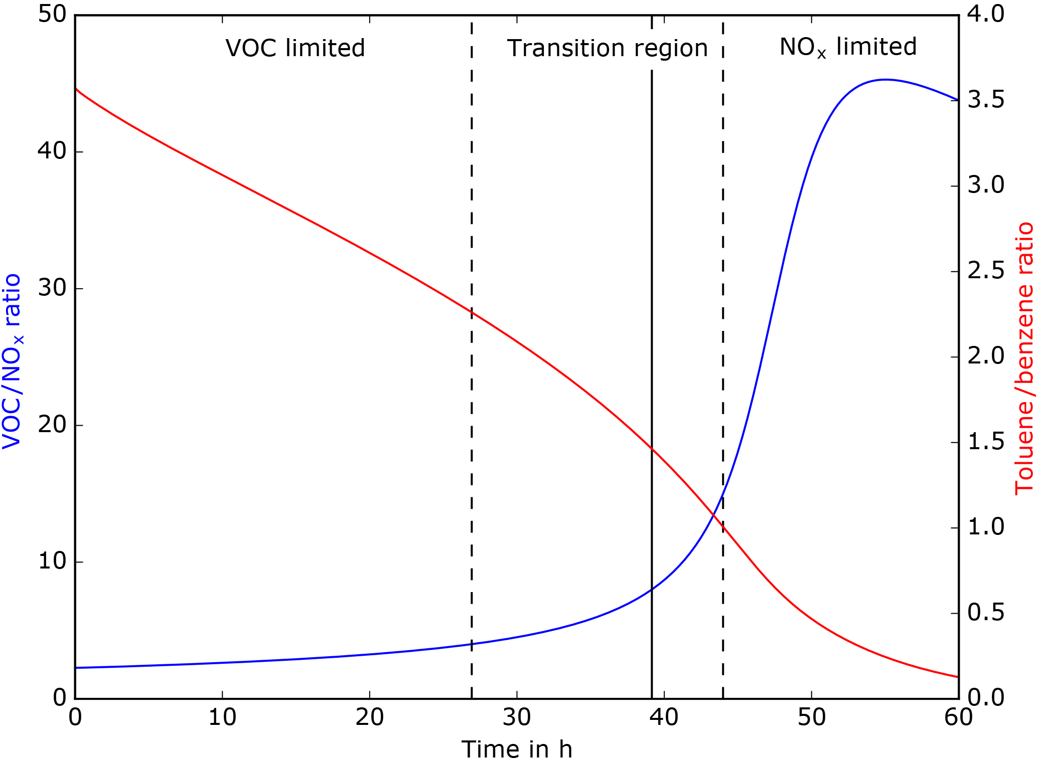
Figure 3Temporal evolution of the VOC ∕ NOx (blue line) and toluene ∕ benzene (red line) ratios over 60 h derived from MOZART-T1 (CR).
The temporal evolutions of some key species in the NR and the CR are displayed in Fig. 4. Nitrogen dioxide (NO2) shows a decrease over time, with a stronger decay in the NR than in the CR. Ozone (O3) production is observed over time with a therefore stronger production in the NR than in the CR. The hydroxyl-radical (OH) availability increases over time, especially between 20 and 35 h, which can be identified as the end of the transition from a VOC-limited to a NOx-limited regime. In the VOC-limited and NOx-limited regimes, the OH increase is smaller. Formaldehyde (CH2O) shows in both NR and CR a decrease followed by an increase and finally a decrease. Those variations illustrate the change of chemical regimes from VOC limited to transition to NOx limited. If we compare the NR to the CR the change of chemical regimes is lagged. The change of regimes seems to occur faster in the NR than in the CR, suggesting different reactivity and pathways of oxidation in the NR than in the CR.
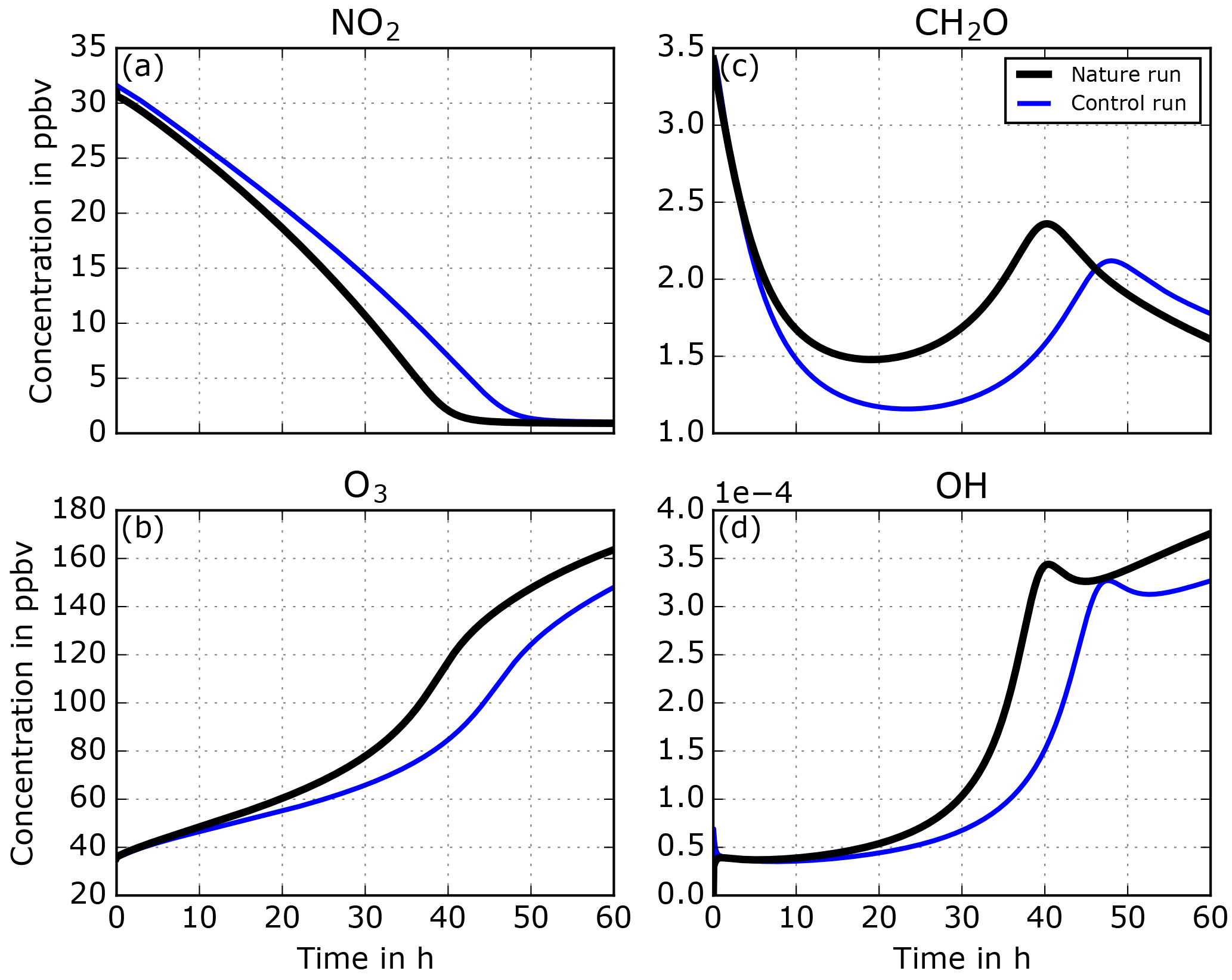
Figure 4Time series of concentrations of NO2, O3, CH2O, and OH over 60 h from the control run (MOZART-T1, blue lines) and from the nature run (MCMv3.3.1, black lines).
3.2 Assimilation runs
We focus on assimilating NO2 and CH2O concentrations in two separate experiments to show the capabilities of the BEATBOX framework. This is motivated by the fact that NO2 and CH2O play a key role in atmospheric chemistry, especially for short-lived chemical compounds. Also, NO2 and CH2O are, and will be, observed from space from both low-Earth and geostationary orbiters and from in situ observations. We define a reduced state vector for simplicity of the demonstration with the species described above: NO2, O3, CH2O, and OH.
We use an assimilation window of 3 h. Unbiased observations have been defined and assumed to be at the end of the assimilation window with an observation error of 0.75 ppbv for NO2 and 0.07 ppbv for CH2O (corresponding to approximately 2.5 and 5 % of the concentrations at initial time). All the generated observations have well-estimated observation error, such as σo=Σ (see Sect. 2.2.2). The model error in the observation space σb has to be specified for the adjoint technique and is set to 2.5 % for NO2 and 5 % for CH2O of the current forecast concentration (see Sect. 2.2.3). For the ensemble method, the ensemble spread implicitly defines σb using 50 ensemble members that are generated by perturbing the initial NO2 concentration by 2.5 % for NO2 assimilation and by perturbing the initial CH2O concentration by 5 % for CH2O assimilation (see Sect. 2.2.4). Adaptive inflation is applied on the ensembles at every assimilation window to maintain a realistic ensemble spread to weight the observation and model appropriately (see Sect. 2.2.6).
3.2.1 NO2 assimilation
We assimilate NO2 observations using two different localizations. The first experiment infers only NO2 concentration and the second infers the entire state vector (i.e., NO2, O3, CH2O, and OH concentrations). After looking at the evolution of NO2 concentrations (see Fig. 5), all three assimilation methods in both experiments (adjoint, ensemble, and hybrid) tend to move the analysis closer toward the observations and hence the NR. Some differences among the three ARs can be found. Recalling Sects. 2.2.1 and 2.2.2, because of the dimensionality of the problem the sensitivity from observation space NO2 to the model variable NO2 is equal to identity, s=1, for every assimilation method. Hence, the difference among assimilation runs will only result from differences in xb and σb after a subsequent forecast. The ensemble and hybrid methods show a quicker improvement than the single member adjoint method due to the adaptive nature of σb with the inflation (see Sect. 2.2.6). The single adjoint method keeps σb=2.5 %, while the ensemble and hybrid methods can tune this value with the inflation.
When only NO2 is inferred the other species are modified and this could be called the model response to assimilated changes: NO2 is decreased, which increases the OH availability for other oxidation pathways. A slight increase in O3 is noted and more significantly for CH2O during the transition region. The ensemble methods have a stronger effect due to the adaptive nature of σb. The adjustment of NO2 concentration towards NO2 observation can be more effective and this can have a stronger effect on the model response.
When the entire state vector is inferred, i.e., no localization, slight additional increases occur in O3, CH2O, and OH in the transition region. In general, in the first 10 to 15 h when VOC-limited conditions dominate (see Fig. 3), the impact of NO2 assimilation is low. By definition, VOC-limited air is insensitive to changes in NO2, so if the model (CR) predicts VOC-limited conditions either adjoint sensitivities or ensemble sensitivity will remain small. After 15 h of simulation, the chemical regime transitions significantly to NOx limited with higher sensitivity of the state to changes in NO2. After 40 h, NO2 concentrations drop to very low values, NO2 assimilation increments are very small, and hence almost no inference on the other state variables is observed.
In the case study, inference from NO2 observation on the rest of vector is not the major reason for improvement. Model response from NO2 changes is mostly responsible for improving the state. NOx concentrations drive the chemistry in the transition region and NOx-limited regimes. NOx chemistry is well known and similarly represented between the NR and the CR. Hence the model response is likely to improve the state and not likely to produce additional errors.
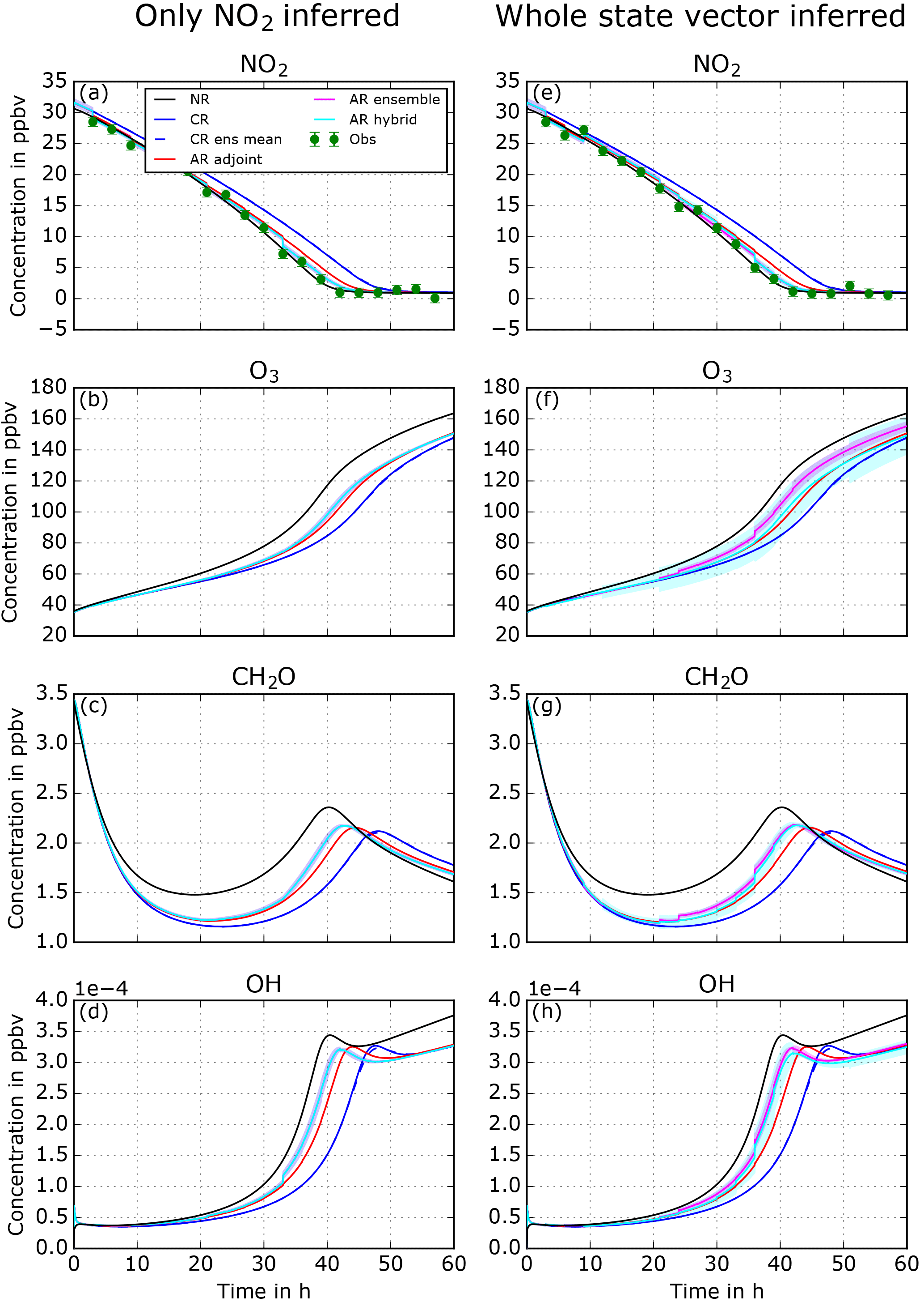
Figure 5Evolution of the state vector over 60 h, including the nature run (NR, black line), control run (CR, blue), and assimilation runs using adjoint (red), ensemble (pink), and hybrid (turquoise) methods. Two experiments with different localizations are displayed: only NO2 inferred (a–d) and whole state vector inferred (e–h). Shaded areas show corresponding ensemble spread for ensemble and hybrid methods.
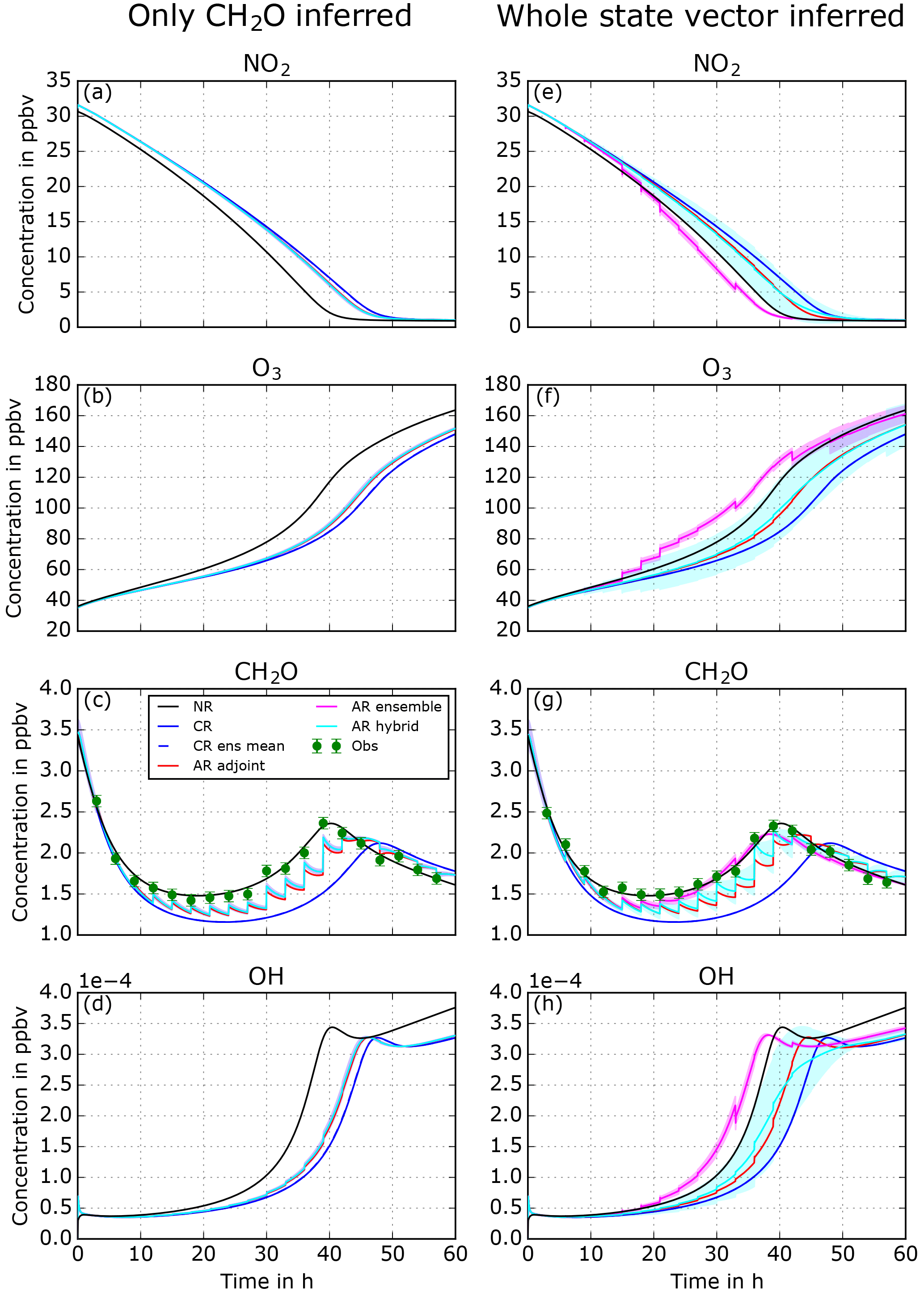
3.2.2 CH2O assimilation
We repeat the experiments presented in Sect. 3.2.1, but assimilate CH2O observations instead of NO2. Figure 6a–d show the concentration evolution when only CH2O is inferred. In the first 40 h CH2O is underestimated by the CR mechanism. All three ARs show very similar results. During the analysis phases the CH2O concentrations are pushed up towards the NR. Those abrupt increases are systematically compensated for by the chemical mechanism nudging the system back into chemical equilibrium, i.e., towards the CR concentrations. This makes the CH2O concentration evolution a sawtooth shape. CH2O is a short-lived chemical compound (shorter than NO2 in this case study) and it is mainly driven by other chemical species concentrations. Ultimately CH2O concentrations in the ARs are slightly elevated after each 3 h forecast. These changes will very mildly affect the state vector concentrations. The model response to CH2O changes in NO2, O3, and OH is slight and definitely smaller than the model response to NO2 changes (see Sect. 3.2.1).
When the entire state vector is inferred, i.e., no localization (Fig. 6e–h), we observe very different results. The two ARs that are using adjoint sensitivities (hybrid and adjoint) show similar results as the previous experiment, and the sawtooth shape is still observed. The analysis shows strong increases in CH2O and the chemical mechanism tries to come back to the CR state. The inference on the other species of the state vector is noticeable, and NO2, O3, and OH concentrations are improved compared to the experiment when only NO2 is inferred.
In the ensemble method in which no localization is applied, the improvement in CH2O is of a different nature. The sawtooth behavior of the AR is not observed anymore and the chemical mechanism now seems to have changed from systematic CH2O loss to CH2O production in the forecast. This will drive the AR to better fit the observations and hence the NR. The inference on other species shows significant changes that will in general change the sign of the error and sometimes increase it; NO2 becomes underestimated in the transition region, O3 is overestimated but then underestimated after 35 h, and OH is overestimated in the transition region. In the ensemble method for the case study, the computed sensitivities seem significantly different from the adjoint sensitivities. This will allow us to change the chemical production and loss rate of CH2O to better adjust the CH2O concentration, but at the risk of disturbing the rest of the state vector and increasing errors that might lead to unphysical results. We diagnose the difference among sensitivities from the two experiments presented above in Sect. 3.3. We also diagnose the chemical behavior change from CH2O assimilation using fluxes in Sect. 3.4.
3.3 Sensitivities of the off-diagonal elements of the background error covariance matrix
Figure 7 shows the sensitivities of the unobserved species to a change in NO2 and CH2O, respectively, at the end of each 3 h assimilation window with the single member adjoint and the ensemble method (see Sects. 2.2.3 and 2.2.4). To make sensitivities comparable we have normalized (divided) them by the state concentrations. For example, s(NO2,O3), the sensitivity of NO2 changes over O3, will most likely be orders of magnitude larger than s(NO2,OH) since O3 concentrations are orders of magnitude larger than OH concentrations.
For NO2 assimilation, both methods deliver similar results. The sensitivities are in general small, not above 60 %. Sensitivities are small or negligible in the VOC-limited regime but become more significant during the transition and the NOx-limited regimes, mostly after 30 h. The changes in NO2 from assimilation after 30 h are rather small and hence the inference on other species will be small. This then confirms that the most important part of the changes from NO2 assimilation is due to the model response from NO2 changes and secondly due to the data assimilation inference on the other species of the state.
For CH2O assimilation we saw significant differences in behavior between adjoint and ensemble methods to compute the sensitivities. The adjoint displays rather small sensitivities, peaking at 20 % but mostly below 10 %. Those sensitives are observed during the VOC-limited regime when the chemistry is sensitive to changes from VOC concentrations and disappear during the transition region and become insignificant in the NOx-limited regime. This explains the small but reasonable impacts from CH2O changes on the rest of the state. Concerning the ensemble method, the computed sensitivities are much larger and do not decrease after the transition regime. Values switch abruptly from negative to positive and are sometimes above 200 %. To understand this unphysical behavior, we display tracer–tracer relationships during the assimilation phase of the ninth cycle (27 h) in Fig. 8.
In Sect. 2.2.4, we defined the ensemble method sensitivity computation as a linear fit to the ensemble distribution between two species. Most state-of-the-art EnKF methods use this approximation. One can see the limitation to such a linear assumption after looking carefully at Fig. 8a and b. The prior and posterior states of the NO2–O3 distributions are displayed. The ensemble method represents the observation well; the ensemble distribution is at the NO2 level of the observation and the ensemble spread fits the observation error (green vertical bars). However, the relationship between NO2 and O3 that has formed during the ensemble AR after nine cycles is strongly curved and nonlinear, which is difficult to represent through the linear fit of the ensemble sensitivity. In this example, moving the ensemble members along the linear fit is moving the O3 distribution slightly away from the NR. At the same time the adjoint sensitivities are in comparison very weak (the slope is along the y axis), slightly improving the state distributions but not very strongly. Finally, the hybrid distribution shows a larger spread and different distribution shape than the ensemble distribution. The adjoint inference does not strongly change the rest of the state, which maintains the chemical production and loss rates of CH2O that fall into a temporary attractor; the model wants to go back to the CR concentrations and creates a sawtooth-shaped concentration evolution over time (see Sect. 3.2.2). After 3 h, the forecast will be significantly far from the observation and the distribution will be inflated. The ensemble inference strongly changes the rest of the state, which will change the chemical production and loss rates and drive the system out of the attractor. To understand this more clearly, the flux tool is presented in the following section.
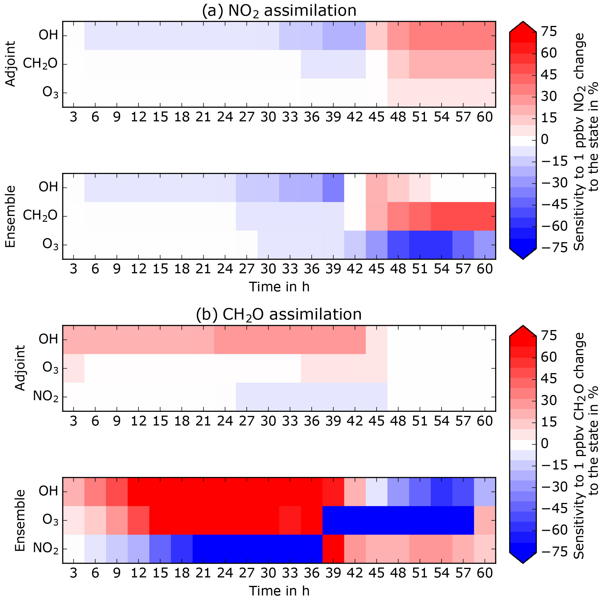
Figure 7Temporal evolution of the sensitivities of the unobserved state species to changes from the observed one at the end of each 3 h assimilation for NO2 assimilation (a) and CH2O assimilation (b).
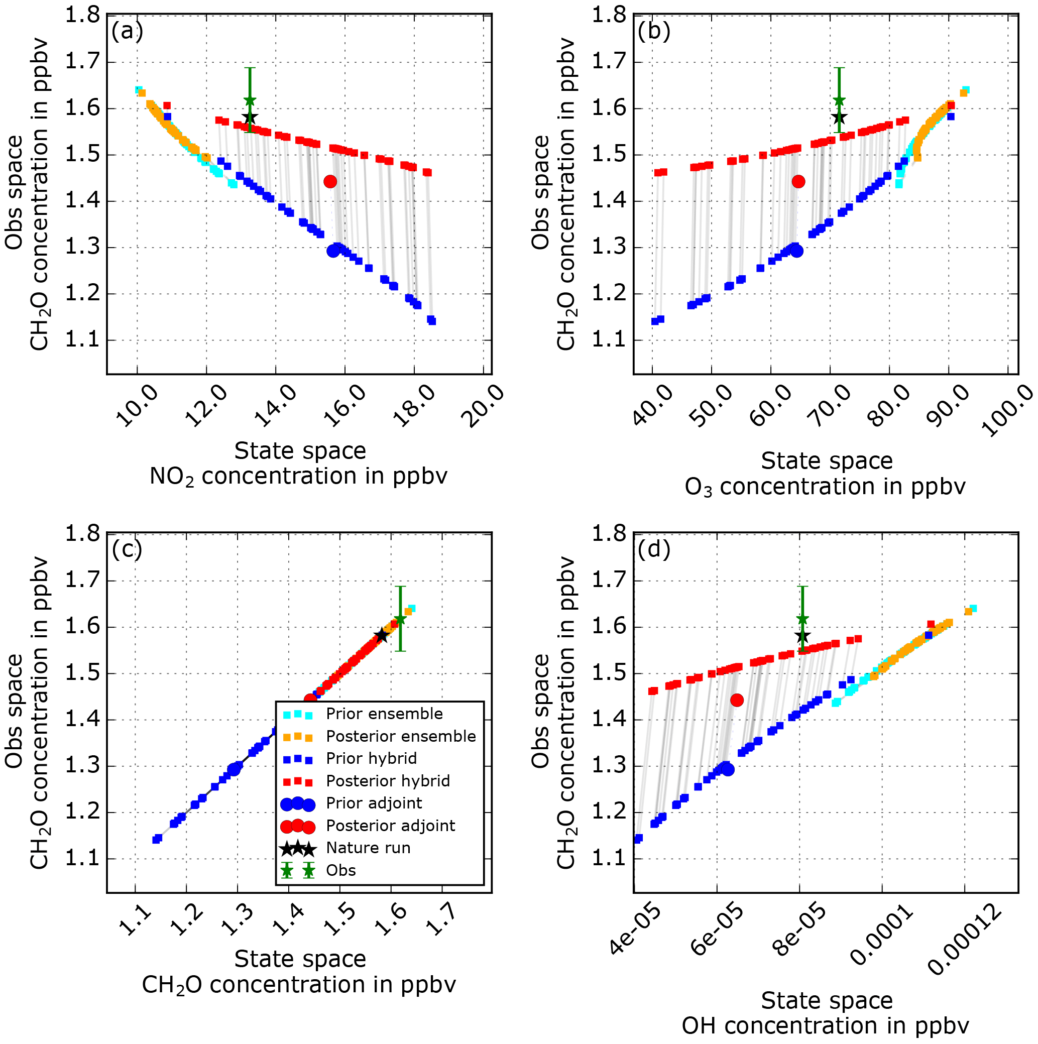
Figure 8Tracer–tracer or observation space to state space relationships during the ninth cycle of the CH2O assimilation without localization experiment.
3.4 Model diagnostics using fluxes
In this last section, we will focus on the CH2O fluxes (production and loss) over the ninth cycle forecast (25 to 27 h) of the CH2O assimilation without localization. In Fig. 9 are the individual contributions of production and loss of CH2O for the NR and the same member of the CR, AR ensemble, and AR hybrid. The flux tool isolates a few different reactions with NR because the chemical scheme is different and more detailed than the CR. In this case study, CH3O → CH2O + HO2 in the NR is simply an intermediate reaction of NO + CH3O2 → CH2O + NO2 + HO2. Other than this reaction, the isolated reactions are similar.
The NR fluxes to the CR fluxes show the same order of production and loss importance; however, the NR fluxes are stronger. Overall the loss terms in the NR are stronger than the CR, leading to a net chemical flux that is negative. The CR rates are significantly faster than the AR ensemble rates, and the slopes of the rates (i.e., the second derivative of the concentration evolution) also differ. The production terms are stronger, leading to almost no loss net flux. The order of importance of the reactions in the budget is also different; CH2O + OH → CO + HO2 + H2O is much more important, likely due to the increase in OH during the AR ensemble (see Sect. 3.2.2). Finally, the AR hybrid fluxes are similar to the CR fluxes with the same order of importance between reactions. Except for the carbon monoxide (CO) formation from photolysis, CH2O → CO + H2 is now stronger and is responsible for the systematic decrease in CH2O in the AR adjoint and AR hybrid (see Sect. 3.2.2). This increased flux from this reaction explains the sawtooth behavior of CH2O. When no other pathway of loss is possible, i.e., OH is not as strongly changed in AR adjoint and hybrid as in AR ensemble, this way of destroying CH2O is then increased.
We demonstrate here the usefulness of the flux tool to diagnose the effect of data assimilation on atmospheric chemistry in a detailed manner. The diagnostic of the flux tool can be used on any species that a chemical scheme contains for any kind of BOXMOX simulation.
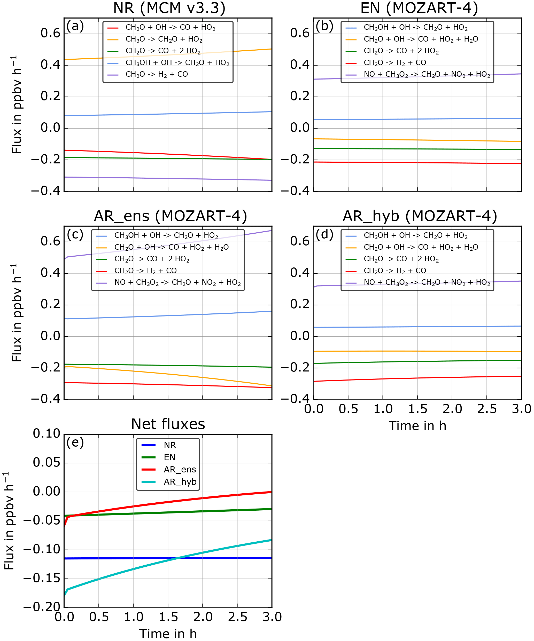
Figure 9CH2O fluxes during the 3 h forecast of the ninth cycle of the CH2O assimilation with no localization. For the NR (a), one member of the CR (b), one member of the AR ensemble (c), and one member of the AR hybrid (d). Net fluxes for each run are shown in panel (e). Displayed are fluxes representative of 90 % of the budget.
In this paper, we have presented a new suite of tools for box models, BEATBOX. The design of BEATBOX is based on an OSSE approach that can simultaneously integrate various chemical schemes to simulate a nature run, control runs, and assimilation runs. This framework includes the capability of running assimilation windows of different chemical schemes using a forecasting tool (BOXMOX) and an assimilation tool allowing for sensitivity analysis. BEATBOX provides ensemble and adjoint sensitivity analyses that can be combined or modified to explore new inverse or data assimilation methodologies. Additionally, a flux tool is also integrated into the framework to diagnose and assess in detail model run differences and ultimately use data assimilation to improve the model (chemical scheme) itself, not only the model outputs. The systematic and detailed assessment of the multivariate data assimilation problem indicates that BEATBOX can tackle important scientific hypotheses at a limited computational cost for future data assimilation configurations in large-scale 3-D models for atmospheric chemistry, but it is not limited to this. Any system of equations can be integrated over time in the current framework.
A typical case study of ozone photochemical production from NOx is presented to showcase the capability of BEATBOX. Differences between the nature run and the control run are presented followed by a data assimilation experiment of synthetic NO2 and CH2O observations using adjoint and ensemble sensitivity analyses with different localization parameters. The case studies shown in this paper illustrate the need to understand in detail the effect of data assimilation in a complicated and nonlinear model as required by atmospheric chemistry. In these case studies, we showcased BEATBOX as a powerful and user-friendly tool for the following:
-
understanding chemical mechanism differences and deficiencies,
-
performing chemical sensitivity analysis using ensemble or adjoint methods,
-
envisioning and designing new inverse and data assimilation methods for atmospheric chemistry to optimally constrain as much of the chemical state as possible,
-
defining requirements for new chemical and data assimilation schemes and ultimately improving them, and
-
educational purposes for data assimilation and atmospheric chemistry.
BEATBOX will continue to evolve according to user requirements. For example, emission inversion capability is currently being implemented. Setting any given observation time into the assimilation window will also be possible. Assimilating multiple observations in a given assimilation window will also be implemented using sequential and variational minimization techniques. Using real observations, i.e., from field campaigns, is also possible with minimal code modifications. Because of the user friendliness, flexibility, and open source nature of most of BOXMOX–BEATBOX, users could also contribute to model development and make it a broad atmospheric chemistry community tool.
All code developments presented here are open source tools released under the GNU General Public License v3. BEATBOX consists of a number of Python packages:
-
beatboxtestbed(the BEATBOX Background Error Analysis Testbed), -
boxmox(Python interface for the chemical box model BOXMOX), -
genbox(input data generator forboxmox), -
frappedata(FRAPPE campaign dataset forgenbox), -
tuv(TUV data connector forgenbox), -
chemspectranslator(translator to translate species between chemical mechanisms and observations), and -
icartt(reader–writer for ICARTT files).
The underlying chemical box model BOXMOX is a stand-alone C and Fortran executable and has to be installed before BEATBOX can be used.
Source code version 1.0 used in this paper is archived online at digital object identifier: 10.5281/zenodo.1118244 (Knote et al., 2017). Full documentation for BOXMOX and all Python packages, including examples on how to reproduce the case studies shown in this paper, can be found at https://boxmodeling.meteo.physik.uni-muenchen.de/documentation.
CK and JB contributed equally to the paper. CK designed the BOXMOX system, wrote the framework around BEATBOX, supervised ME, and contributed to writing the paper. JB came up with the idea for BEATBOX and coded most of the beatbox.py routine, co-supervised ME, and wrote most of the paper. ME developed parts of the BEATBOX framework during his Masters thesis, prepared and analyzed the case studies, and contributed the flux tool.
The authors declare that they have no conflict of interest.
We thank the many scientists who contributed to the FRAPPE field campaign for
providing useful data to initialize the model simulations. Frank Flocke and
Rebecca Hornbrook (NCAR) are thanked for creating the Commerce City
sample used in the case studies. We acknowledge Bill Carter (UC Riverside)
for his work on the emission database. We acknowledge support from NASA
KORUS-AQ grant NNX16AD96G.
Edited by: Tim
Butler
Reviewed by: two anonymous referees
Anderson, J. L.: A local least squares framework for ensemble filtering, Mon. Weather Rev., 131, 634–642, 2003.
Anderson, J. L.: An adaptive covariance inflation error correction algorithm for ensemble filters, Tellus A, 59, 210–224, 2007.
Archibald, A. T., Jenkin, M. E., and Shallcross, D. E.: An isoprene mechanism intercomparison, Atmos. Environ., 44, 5356–5364, https://doi.org/10.1016/j.atmosenv.2009.09.016, 2010.
Arnold, C. P. and Dey, C. H.: Observing-systems simulation experiments: Past, present, and future, B. Amer. Meteorol. Soc., 67, 687–695, 1986.
Barré, J., Edwards, D., Worden, H., Silva, A. D., and Lahoz, W.: On the feasibility of monitoring carbon monoxide in the lower troposphere from a constellation of northern hemisphere geostationary satellites (part 1). Atmos. Environ., 113, 63–77, 2015.
Barré, J., Edwards, D., Worden, H., Arellano, A., Gaubert, B., Silva, A. D., Lahoz, W., and Anderson, J.: On the feasibility of monitoring carbon monoxide in the lower troposphere from a constellation of northern hemisphere geostationary satellites: Global scale assimilation experiments (part II), Atmos. Environ., 140, 188–201, 2016.
Claeyman, M., Attié, J.-L., Peuch, V.-H., El Amraoui, L., Lahoz, W. A., Josse, B., Joly, M., Barré, J., Ricaud, P., Massart, S., Piacentini, A., von Clarmann, T., Höpfner, M., Orphal, J., Flaud, J.-M., and Edwards, D. P.: A thermal infrared instrument onboard a geostationary platform for CO and O3 measurements in the lowermost troposphere: Observing System Simulation Experiments (OSSE), Atmos. Meas. Tech., 4, 1637–1661, https://doi.org/10.5194/amt-4-1637-2011, 2011.
Coates, J. and Butler, T. M.: A comparison of chemical mechanisms using tagged ozone production potential (TOPP) analysis, Atmos. Chem. Phys., 15, 8795-8808, https://doi.org/10.5194/acp-15-8795-2015, 2015.
Edwards, D. P., Arellano Jr., A. F., and Deeter, M. N.: A satellite observation system simulation experiment for carbon monoxide in the lowermost troposphere, J. Geophys. Res., 114, D14304, https://doi.org/10.1029/2008JD011375, 2009.
Emmerson, K. M. and Evans, M. J.: Comparison of tropospheric gas-phase chemistry schemes for use within global models, Atmos. Chem. Phys., 9, 1831–1845, https://doi.org/10.5194/acp-9-1831-2009, 2009.
Emmons, L. K., Walters, S., Hess, P. G., Lamarque, J.-F., Pfister, G. G., Fillmore, D., Granier, C., Guenther, A., Kinnison, D., Laepple, T., Orlando, J., Tie, X., Tyndall, G., Wiedinmyer, C., Baughcum, S. L., and Kloster, S.: Description and evaluation of the Model for Ozone and Related chemical Tracers, version 4 (MOZART-4), Geosci. Model Dev., 3, 43–67, https://doi.org/10.5194/gmd-3-43-2010, 2010.
Fitzgerald, R.: Divergence of the Kalman filter, IEEE T. Automat. Contr., 16, 736–747, 1971.
Jenkin, M. E., Young, J. C., and Rickard, A. R.: The MCM v3.3.1 degradation scheme for isoprene, Atmos. Chem. Phys., 15, 11433–11459, https://doi.org/10.5194/acp-15-11433-2015, 2015.
Knote, C., Hodzic, A., Jimenez, J. L., Volkamer, R., Orlando, J. J., Baidar, S., Brioude, J., Fast, J., Gentner, D. R., Goldstein, A. H., Hayes, P. L., Knighton, W. B., Oetjen, H., Setyan, A., Stark, H., Thalman, R., Tyndall, G., Washenfelder, R., Waxman, E., and Zhang, Q.: Simulation of semi-explicit mechanisms of SOA formation from glyoxal in aerosol in a 3-D model, Atmos. Chem. Phys., 14, 6213–6239, https://doi.org/10.5194/acp-14-6213-2014, 2014.
Knote, C., Tuccella, P., Curci, G., Emmons, L., Orlando, J. J., Madronich, S., Barò, R., Jimènez-Guerrero, P., Luecken, D., Hogrefe, C., Forkel, R., Werhahn, J., Hirtl, M., Pèrez, J. L., San Josè, R., Giordano, L., Brunner, D., Yahya, K., and Zhang, Y.: Influence of the choice of gas-phase mechanism on predictions of key gaseous pollutants during the AQMEII phase-2 intercomparison, Atmos. Environ., 115, 553–568, 2015.
Knote, C., Barré, J., and Eckl, M.: BEATBOX v1.0: Background Error Analysis Testbed with Box Models (Version 1.0.0), Zenodo, https://doi.org/10.5281/zenodo.1118244, 19 December 2017.
Kuo, Y.-H., Zou, X., and Huang, W.: The impact of global positioning system data on the prediction of an extratropical cyclone: an observing system simulation experiment, Dynam. Atmos. Oceans, 27, 439–470, 1998.
Lahoz, W., Khattatov, B., and Mènard, R. (Eds.): Data Assimilation: Making Sense of Observations, Springer Berlin Heidelberg, 718 pp., 2010.
Liu, C., Xiao, Q., and Wang, B.: An ensemble-based four-dimensional variational data assimilation scheme, part II: Observing system simulation experiments with advanced research WRF (ARW), Mon. Weather Rev., 137, 1687–1704, 2009.
Madronich, S. and Flocke, S.: Theoretical Estimation of Biologically Effective UV Radiation at the Earth's Surface, Springer, Berlin Heidelberg, 23–48, 1997.
Mazzuca, G. M., Ren, X., Loughner, C. P., Estes, M., Crawford, J. H., Pickering, K. E., Weinheimer, A. J., and Dickerson, R. R.: Ozone production and its sensitivity to NOx and VOCs: results from the DISCOVER-AQ field experiment, Houston 2013, Atmos. Chem. Phys., 16, 14463–14474, https://doi.org/10.5194/acp-16-14463-2016, 2016.
Mitchell, H. L. and Houtekamer, P. L.: An adaptive ensemble Kalman filter, Mon. Weather Rev., 128, 416–433, 2000.
Nichols, N. K.: Mathematical Concepts of Data Assimilation, in: Data assimilation: making sense of observations, edited by: Lahoz, W., Khattatov, B. and Menard, R., Springer, 13–39, 2010.
Ott, E., Hunt, B., Szunyogh, I., Zimin, A., Kostelich, E., Corrazza, M., Kalnay, E., and Yorke, J.: A local ensemble Kalman filter for atmospheric data assimilation, Tellus A, 56, 415–428, 2004.
Sandu, A. and Sander, R.: Technical note: Simulating chemical systems in Fortran90 and Matlab with the Kinetic PreProcessor KPP-2.1, Atmos. Chem. Phys., 6, 187–195, https://doi.org/10.5194/acp-6-187-2006, 2006.
Sandu, A., Daescu D., and Carmichael G. R.: Direct and adjoint sensitivity analysis of chemical kinetic systems with KPP: Part I – theory and software tools, Atmos. Environ., 37, 5083–5096, https://doi.org/10.1016/j.atmosenv.2003.08.019, 2003.
Sandu, A., Daescu, D. N., Carmichael, G. R., and Chai, T.: Adjoint sensitivity analysis of regional air quality models, J. Comput. Phys., 204, 222–252, 2005.
van Leeuwen, P. J.: Nonlinear data assimilation in geosciences: an extremely efficient particle filter, Q. J. Roy. Meteor. Soc., 136, 1991–1999, https://doi.org/10.1002/qj.699, 2010.
Wang, X., Barker, D. M., Snyder, C., and Hamill, T. M.: A hybrid ETKF-3DVar data assimilation scheme for the WRF model, Part I: Observing system simulation experiment, Mon. Weather Rev., 136, 5116–5131, 2008.
Wolfe, G. M., Marvin, M. R., Roberts, S. J., Travis, K. R., and Liao, J.: The Framework for 0-D Atmospheric Modeling (F0AM) v3.1, Geosci. Model Dev., 9, 3309–3319, https://doi.org/10.5194/gmd-9-3309-2016, 2016.