2.1 General structure of the atmosphere

Aeolus 1.0 is a 2.5-D SD model, with the vertical dimension being largely parameterized and only coarsely resolved, and it therefore belongs to the class of intermediate complexity atmosphere models. Water and energy conservation is achieved via a set of two-dimensional, vertically averaged prognostic equations for temperature and specific humidity (Petoukhov et al., 2000).

The three-dimensional structure is described by these two-dimensional surface fields with the vertical dimensions reconstructed using an equation for the lapse rate and assuming an exponential profile for specific humidity (Petoukhov et al., 2000).

For given temperature and specific humidity fields, the three-dimensional wind field is calculated using a set of diagnostic equations. These statistical–dynamical equations for the wind fields are coupled and thus need several time steps or iterations to equilibrate.

The equations of the dynamical core of Aeolus 1.0 are separated into equations for the (1) synoptic-scale transient waves (or storm tracks), (2) quasi-stationary planetary waves and (3) the zonal-mean wind. Thus, following classical statistical–dynamical approaches (Dobrovolski, 2000; Imkeller and von Storch, 2012), the key assumption is that the wind velocity field V can be split into a synoptic-scale component V^′ (2- to 6-day period) and a large-scale, long-term component 〈V〉 (Fraedrich and Böttger, 1978) such that

The variables u, v and w describe the wind velocity in zonal, meridional and vertical directions. The brackets (〈…〉) symbolize time-averaged quantities and the prime (…^′) indicates deviations from this time-averaged field. The large-scale long-term component 〈V〉 is subdivided into a zonal-mean $\stackrel{\mathrm{‾}}{\langle V\rangle }$ and an azonal component 〈V^∗〉 :

The large-scale, zonal-mean zonal wind velocity $\stackrel{\mathrm{‾}}{\langle u\left(z,\mathit{\varphi }\right)\rangle }$ with height above surface z and latitude ϕ is assumed to be geostrophic (resulting in the thermal wind balance):

where the sea level pressure gradient is calculated by $\langle \frac{\stackrel{\mathrm{‾}}{\partial p_{\mathrm{0}}}}{\partial \mathit{\varphi }}\rangle =\frac{a{v}^{\ast }\mathit{\rho }\mathrm{|}f\mathrm{|}}{-C_{\mathit{\alpha }}\sin \mathit{\alpha }}$ with ageostrophic velocity parameter C_α=5 and the Earth radius a (derived and explained by Pethoukov et al. 2000; Eq. 13) and α is the cross-isobar angle defined as in Coumou et al. (2011; their Eq. A31). The variable v^∗ is the azonal meridional wind velocity, ρ is the air density with the reference air density ρ₀, f is the Coriolis parameter, ϕ is the latitude, T₀ is the reference temperature and g is the gravitational acceleration (see Petoukhov et al., 2000).

As derived in the Supplement in Sect. S2, the large-scale, zonal-mean meridional wind velocity $\stackrel{\mathrm{‾}}{\langle v\left(z,\mathit{\varphi }\right)\rangle }$ is given by

where $d_{\mathrm{1}},d_{\mathrm{2}},d_{\mathrm{3}},d_{\mathrm{4}},n_{\mathrm{1}},n_{\mathrm{2}}$ and n₃ are tunable parameters and A represents the convection-related term:

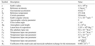
The atmospheric-scale height H₀, the exchange for the momentums K_z, the Earth's angular velocity Ω as well as the dry adiabatic lapse rate Γ_a, latent heat of evaporation L and model parameters ${\mathrm{\Gamma }}_{\mathrm{0}},{\mathrm{\Gamma }}_{\mathrm{1}},{\mathrm{\Gamma }}_{\mathrm{2}},a_q,T_{\mathrm{0}}$ are explained in Table 1. T_a is a temperature which would occur near the surface if the lapse rate did not change within the planetary boundary layer (PBL), q_s is the surface air specific humidity and n_c is the cumulus cloud amount. The latter variable is either computed by the cloud module or, as in this experiment, observational data are used. The variable P_co is the convective precipitation rate and is calculated by the cloud model (Eliseev et al., 2013). The variable u_sf is the zonal surface wind; see Eq. (S10) in the Supplement.

Table 1Atmosphere model parameters.

Download Print Version | Download XLSX

The azonal component of the large-scale wind field describes quasi-stationary planetary waves and depends on latitude, longitude and height. At the equivalent barotropic level (EBL), azonal geostrophic components of horizontal velocities are computed by employing the definition of the stream function ψ depending on latitude ϕ and longitude λ:

whereby the stream function can be subdivided into contributions from thermally and orographically induced waves depicted by subscripts “th” and “or”, respectively. They are considered to be additive due to linearity of the barotropic vorticity equations such that

The parameter Ψ₀ is a tuning parameter which is necessary since smoothing is applied to dampen local moisture feedbacks in the model. This smoothing however reduces spatial gradients in ${\mathit{\psi }}_{\mathrm{EBL}}^{\ast }$ and therefore $u_{\mathrm{EBL}}^{\ast }$ and $v_{\mathrm{EBL}}^{\ast }$ themselves. The equation for the orographically induced waves is introduced in Sect. S1.2 in the Supplement.

The zeroth-order solution of the thermally induced waves of the barotropic vorticity equation is given by (see Sect. S1.3 in the Supplement)

It is solved at two beta planes, for the Northern Hemisphere and Southern Hemisphere, respectively:

The beta plane is an approximation in which the Coriolis parameter is linearized to reference latitudes β_NH and β_SH for the Northern Hemisphere and Southern Hemisphere, respectively. In the tropical belt, the variable $\langle {\mathit{\psi }}_{\mathrm{th},\mathrm{0},\mathrm{EBL}}^{\ast }\rangle$ is interpolated linearly between the two beta planes.

The standardized integrated heat content in Eq. (8) $(I_v={\int }_{\mathrm{0}}^{z_{\mathrm{EBL}}}\mathit{\rho }\langle \left[T\left(z\right)\right]\rangle \mathrm{d}z)$ is calculated analytically by assuming a lapse rate $\mathrm{\Gamma }={\mathrm{\Gamma }}_{\mathrm{0}}+{\mathrm{\Gamma }}_{\mathrm{1}}\left(T_{\mathrm{a}}-T_{\mathrm{0}}\right)\left(\mathrm{1}-a_q{q}_{\mathrm{s}}^{\mathrm{2}}\right)-{\mathrm{\Gamma }}_{\mathrm{2}}{n}_{\mathrm{c}}$ such that $T\left(z\right)=T\left(z_{\mathrm{EBL}}\right)-\mathrm{\Gamma }\left(z-z_{\mathrm{EBL}}\right)$. One obtains

In addition, I_v is smoothed by five points in latitude to avoid numerical artifacts which may arise due to spatial differentiating.

To remove possible singularities near the poles, at high latitudes, the stream function is dampened by a fourth-order interpolation function. Planetary waves at other tropospheric levels are directly calculated from those at the EBL (see Sect. S1.1 in the Supplement).

Finally, the time-averaged kinetic energy of transient eddies $\langle E_k^{\prime }\rangle =\frac{\mathrm{1}}{\mathrm{2}}\left(\langle {u^{\prime }}^{\mathrm{2}}\rangle +\langle {v^{\prime }}^{\mathrm{2}}\rangle \right)$ is determined using the statistical–dynamical equations as described in Coumou et al. (2011). Since detailed derivations are provided in Coumou et al. (2011), we only briefly discuss the diagnostic equations for transient eddy activity here. The equations are derived starting from the equation of the kinetic energy of transient eddies:

By assuming that the vertical (baroclinic) flux term is equipartitioned between the zonal and the meridional kinetic energy components, we can split Eq. (11) into three separate equations for $\langle {u^{\prime }}^{\mathrm{2}}\rangle$, $\langle {v^{\prime }}^{\mathrm{2}}\rangle$ and $\langle u^{\prime }{v}^{\prime }\rangle$:

Here, K_fh and K_fz are internal atmospheric small-/mesoscale friction coefficients in the horizontal and vertical directions, respectively; K_fs is the surface friction coefficient; f is the Coriolis parameter; and the subscript “ag” denotes ageostrophic terms.

The terms for K_syn, the vertical macro-turbulent diffusion coefficient and $f\left(\langle v^{\prime }{v}_{\mathrm{ag}}^{\prime }\rangle -\langle u^{\prime }{u}_{\mathrm{ag}}^{\prime }\rangle \right)$, need to be parameterized, which is derived in Coumou et al. (2011). This way, a set of diagnostic equations for synoptic transient eddies is derived which, as also seen in Eqs. (12)–(14), are all coupled to the large-scale wind field.

This provides us with a coupled set of equations for $\stackrel{\mathrm{‾}}{\langle u\rangle },\stackrel{\mathrm{‾}}{\langle v\rangle },\langle u^{\ast }\rangle ,\langle v^{\ast }\rangle ,\langle {u^{\prime }}^{\mathrm{2}}\rangle ,\langle {v^{\prime }}^{\mathrm{2}}\rangle$ and $\langle u^{\prime }{v}^{\prime }\rangle$, which can be solved. Cross terms like $\stackrel{\mathrm{‾}}{\langle u^{\ast }{v}^{\ast }\rangle }$ can be determined by multiplying 〈u^∗〉 with 〈v^∗〉 and taking the zonal mean of that quantity. All derivatives are determined numerically. The values of the parameters are listed in Table 1.

5.1 Dynamical core tuning – step 1

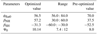
For a good starting point, the parameters are first tuned manually, providing “pre-optimized” values. Next, we define physically realistic parameter ranges for automatic tuning as listed in Table 2.

Table 2Pre-optimized and optimized parameter sets and parameter ranges for optimization step 1.

Download Print Version | Download XLSX

For the azonal wind velocities, we use a weighting function which excludes the tropics (from 10^∘ S to 10^∘ N) and polar regions (poleward of 60^∘ S for the Southern Hemisphere to exclude influences of Antarctica and poleward of 70^∘ N for the Northern Hemisphere) such that the midlatitudes, where planetary waves are important, are optimized.

The non-excluded grid as well as the zonal-mean zonal wind are weighted by w(ϕ)=|cos (ϕ)|.

The total skill score for the scheme in step 1 is calculated by multiplying the individual skills for the azonal velocities in zonal and meridional directions $(S_{u^{\ast }},S_{v^{\ast }})$ and the skill for the zonal-mean zonal wind velocity$\left(S_{\stackrel{\mathrm{‾}}{\langle u\rangle }}\right)$:

The goal of the optimization procedure is to maximize the skill S.

Skill score functions for individual variables are computed as in Taylor (2001):

In Eq. (15), r_X is the coefficient of the spatial correlation between the area-weighted modeled and observed fields of X; A_X is the so-called relative spatial variation calculated according to

Here, the variable A_X,M is the spatial average of $\left|X_{\mathrm{M}}-X_{\mathrm{M},\mathrm{g}}\right|$ and X_M,g is a globally averaged value of the modeled field X_M. The observed field is similarly defined by A_X,O.

5.2 Dynamical core tuning – step 2

For tuning the zonal-mean meridional wind velocity $\stackrel{\mathrm{‾}}{\langle v\rangle }$, and in particular the strength and width of the Hadley cell, we use the vertical integral of the lower tropospheric integrated mass flux $\stackrel{\mathrm{‾}}{\langle m\rangle }$. In addition, we tune the zonal-mean area-weighted synoptic kinetic energy $\langle E_k^{\prime }\rangle$. Both variables strongly depend on the dynamic fields tuned in step 1, which is the reason for tuning them in a separate second step.

Total skill score for the scheme in step 2 is calculated by multiplying the individual skills for the vertical integral of lower troposphere mass flux $\left(S_{\stackrel{\mathrm{‾}}{\langle m\rangle }}\right)$ as well as the eddy kinetic energy $\left(S_{\langle E_k^{\prime }\rangle }\right)$:

The goal of the optimization procedure is again to maximize skill S.

The skill score function for the eddy kinetic energy is given by the Taylor skill score function (Eq. 15).

The skill score is then calculated by

Here, r_X is the coefficient of the spatial correlation between area-weighted modeled and observed fields (as in Eq. 15), mean_{Hadley_Model} and mean_{Hadley_Obs} are the mean values of the area-weighted modeled and observed mean mass flux. We use this more elaborate skill function to promote a proper Hadley circulation in the model.

The weights of the lower troposphere mass flux $\stackrel{\mathrm{‾}}{\langle m\rangle }$ are calculated according to

For calculating the mean intensity of the Hadley cell, we determine the roots of the mass flux in observation data close to 0 and 30^∘ which determine the Hadley cell latitudinal boundaries. This way, we have 36 values for the boundaries of the northern Hadley cell. Between these latitudinal borders, we calculate the mean strength of the Hadley cell.

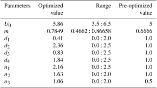
In Table 3, the manually tuned (or pre-optimized) parameters and their ranges are listed.

Table 3Pre-optimized and optimized parameter sets and parameter ranges for optimization step 2.

Download Print Version | Download XLSX

6.1 Results of calibration – step 1

We compared the numerical solutions using the optimized parameters for the wind fields 〈u^∗〉, 〈v^∗〉 and $\stackrel{\mathrm{‾}}{\langle u\rangle }$ of climatological monthly averages, El Niño and La Niña months from ERA-Interim reanalysis (Dee et al., 2011) for 1983–2009.

The figures for azonal wind velocities are divided into six subplots. The left column shows observational data and the right column model data. The top row shows climatological monthly averages, the middle row multiyear averages of El Niño months and the bottom row multiyear averages of La Niña months.

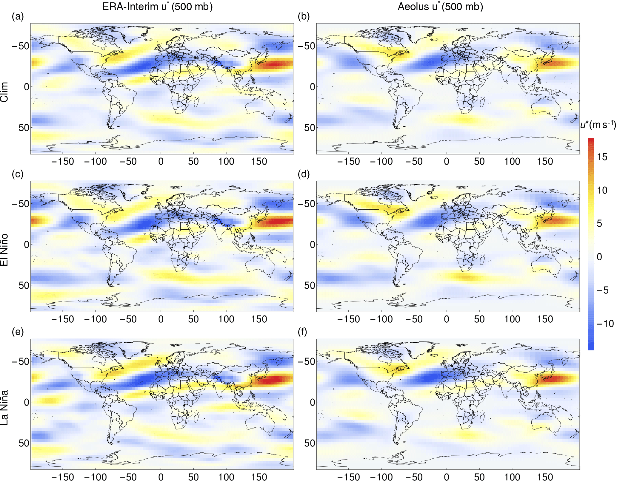
Figure 1Azonal large-scale zonal wind u^* at 500 mb for all February months/El Niño February months/La Niña February months. The left column shows the results from reanalysis data and the right column shows the results from Aeolus received by optimized parameters. The model is forced by surface temperature, humidity and cumulus cloud fraction.

Download

Figure 2Azonal large-scale zonal wind velocity u^∗ at 500 mb for August (compare Fig. 1).

Download

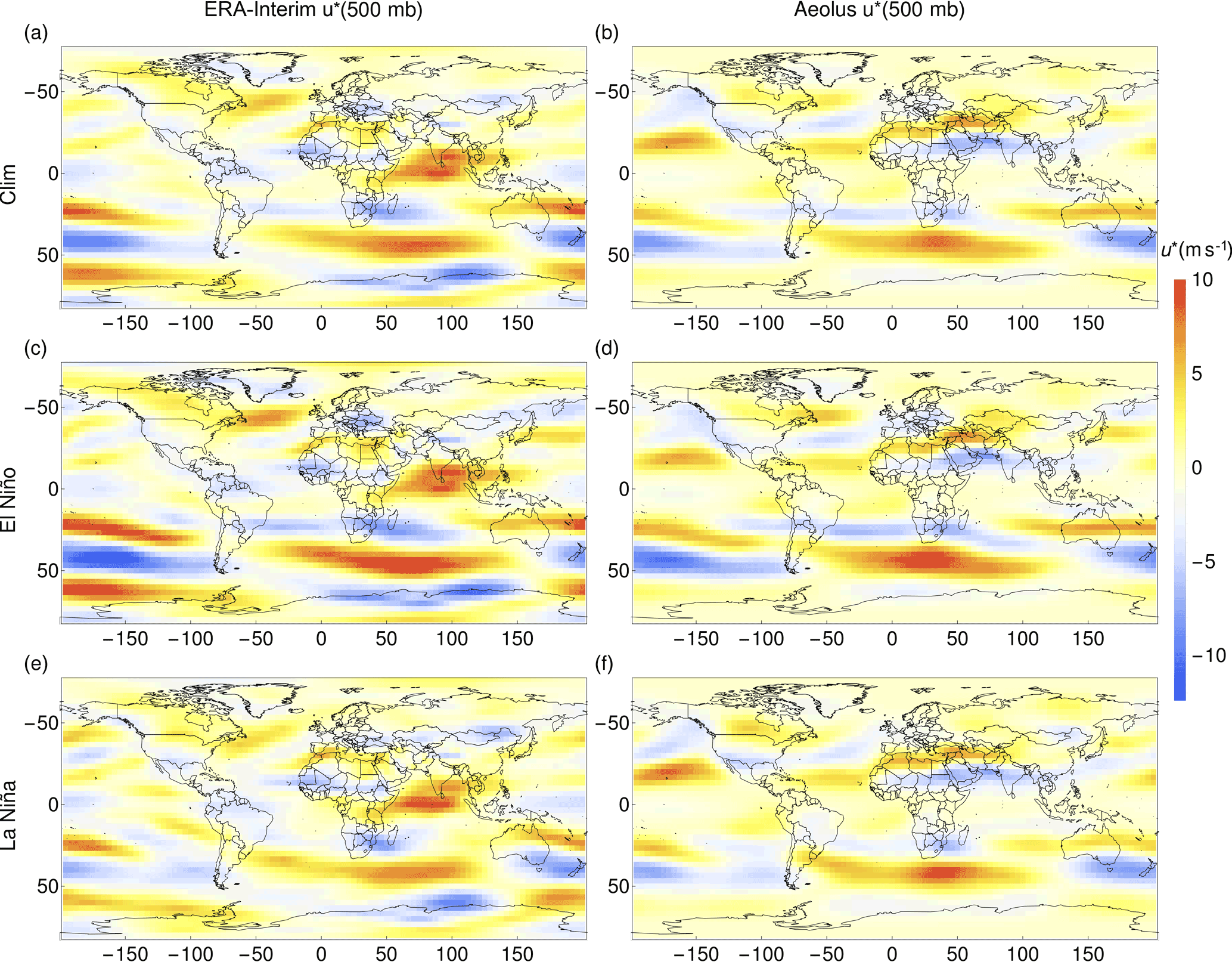
In Figs. 1 and 2, the azonal components of the zonal wind velocities (〈u^∗〉) for February and August at 500 mb are displayed, respectively. The figures show that with optimized parameters the model reasonably reproduces the main observed features both in terms of spatial position and magnitude. In particular, the extratropical planetary waves are well captured with some minor discrepancies in the tropics. Both the seasonal cycle and the response to the ENSO cycle are well captured by the model.

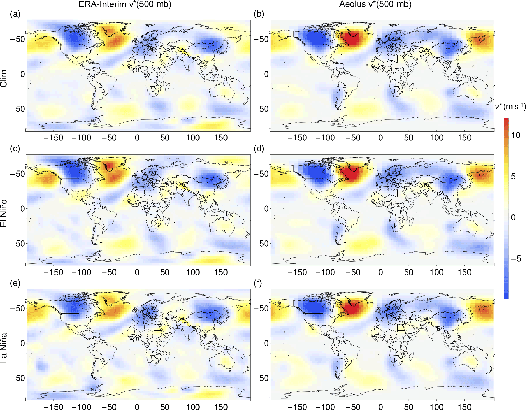
Figure 3Azonal large-scale meridional wind velocity v^∗ at 500 mb for February (compare Fig. 1).

Download

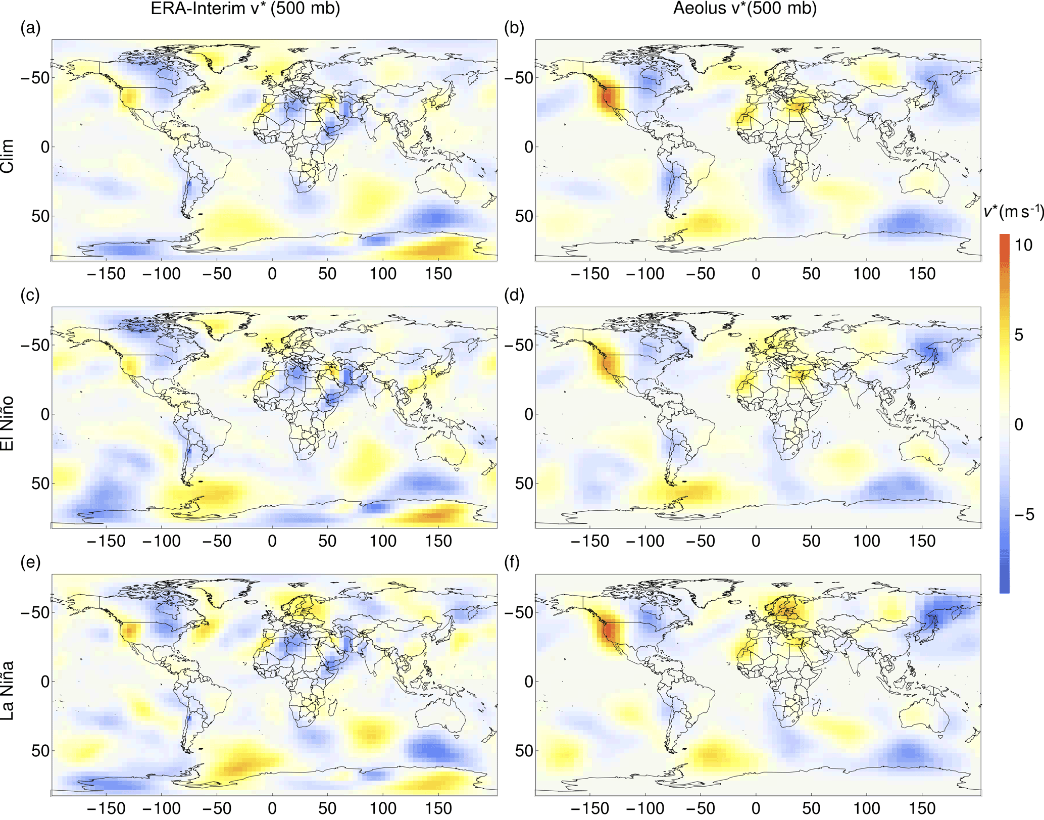
Figure 4Azonal large-scale meridional wind velocity v^∗ at 500 mb for August (compare Fig. 1).

Download

Figures 3 and 4 show the same type of plots for the azonal meridional wind velocity (〈v^∗〉). Also, for the meridional wind velocity, the most important features of the reanalysis data are well represented in the model. The model results coincide well in wind strength and spatial pattern with the reanalysis data. The wind strength in winter, for both climatological and El Niño months, is stronger than for La Niña months. In summer, the opposite is seen for both model and reanalysis data.

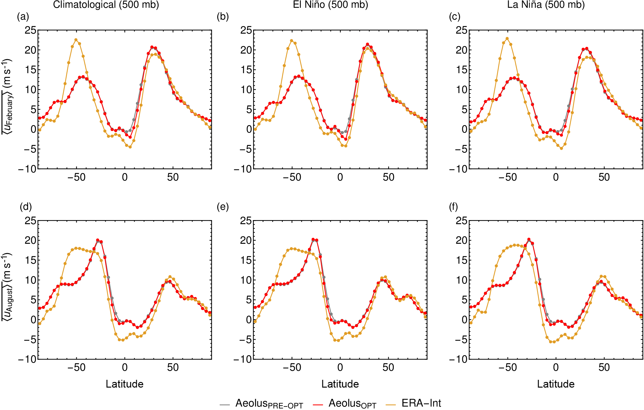
Figure 5Zonal-mean large-scale zonal wind velocity $\stackrel{\mathrm{‾}}{\langle u\left(z,\mathit{\varphi }\right)\rangle }$ at 500 mb. Panel (a) shows the climatological monthly mean zonal-mean zonal velocity in February, (b) the monthly mean zonal-mean velocity of El Niño February months and (c) the monthly mean zonal-mean velocity of La Niña February months. Panel (d) displays the monthly mean climatological zonal-mean zonal velocity in August, (e) the monthly mean zonal-mean velocity in El Niño August months and (f) the monthly mean zonal-mean velocity in La Niña August months. The yellow line represents zonal-mean large-scale zonal wind obtained by reanalysis data, the gray line is zonal-mean large-scale zonal wind velocity from Aeolus using pre-optimized parameters and the red line represents zonal-mean large-scale zonal wind velocity from Aeolus using optimized parameters.

Download

In Fig. 5, the zonal-mean zonal wind velocity $\left(\stackrel{\mathrm{‾}}{\langle u\rangle }\right)$ at 500 mb is shown with the orange line representing reanalysis data, red representing model data with optimized parameters and gray representing model data with pre-optimized parameters. The figure is subdivided into six subplots. The top row depicts $\stackrel{\mathrm{‾}}{\langle u\rangle }$ in February and the bottom row shows $\stackrel{\mathrm{‾}}{\langle u\rangle }$ in August, while the columns show climatological data, El Niño data and La Niña data, respectively. It is noticeable that the results obtained with pre-optimized parameters are already reasonable. Apparently, the initial choice of tuning parameter values was already near the optimum, and hence the optimized parameters led only to small improvements of the model results. The Northern Hemisphere $\stackrel{\mathrm{‾}}{\langle u\rangle }$ profile is well resolved in both seasons for both El Niño and La Niña months. Parameter optimization slightly improves the results in the tropics. The modeled amplitude of $\stackrel{\mathrm{‾}}{\langle u\rangle }$ in the Southern Hemisphere is too small in February for all plots and too high in August.

The optimized parameters are listed in Table 2. The β_NH in the Northern Hemisphere has a higher value, whereas the β_SH in the Southern Hemisphere has a lower value than the pre-optimized parameter values.

The last parameter is Ψ₀ and is changed to a higher value in order to strengthen speeds in 〈v^∗〉 and 〈u^∗〉.

6.2 Results of calibration – step 2

We compared the numerical solutions using the optimized parameters for the zonal-mean lower troposphere integrated mass flux $\stackrel{\mathrm{‾}}{\langle m\rangle }$ and eddy kinetic energy $\stackrel{\mathrm{‾}}{\langle E_k^{\prime }\rangle }$

Figure 6Zonal-mean large-scale mass flux $\stackrel{\mathrm{‾}}{\langle m\rangle }$. Panel (a) shows the climatological monthly mean zonal-mean mass flux in February, (b) the monthly mean zonal-mean mass flux of El Niño February months and (c) the monthly mean zonal-mean mass flux of La Niña February months. Panel (d) displays the monthly mean climatological zonal-mean mass flux in August, (e) the monthly mean zonal-mean mass flux in El Niño August months and (f) the monthly mean zonal-mean mass flux in La Niña August months. The yellow line represents zonal-mean large-scale mass flux obtained by reanalysis data, the gray line is the zonal-mean large-scale mass flux from Aeolus using pre-optimized parameters and the red line represents the zonal-mean large-scale mass flux from Aeolus using optimized parameters.

Download

The plots in Fig. 6 show that in general the monthly mean zonal-mean mass flux calculated with optimized parameters matches better with observational data. Here, the gain of the parameter optimization is clearly better than we saw with calibration step 1. The ENSO cycle is clearly visible. However, the width of the Hadley cell (especially in August) is still too small compared to the width of the Hadley cell obtained by reanalysis data. The figure shows only plots with a latitudinal range from 60^∘ S to 90^∘ N as reanalysis data are spiky over Antarctica.

Figure 7Zonal-mean time-averaged eddy kinetic energy $\stackrel{\mathrm{‾}}{\langle E_k^{\prime }\rangle }$ (compare Fig. 6).

Download

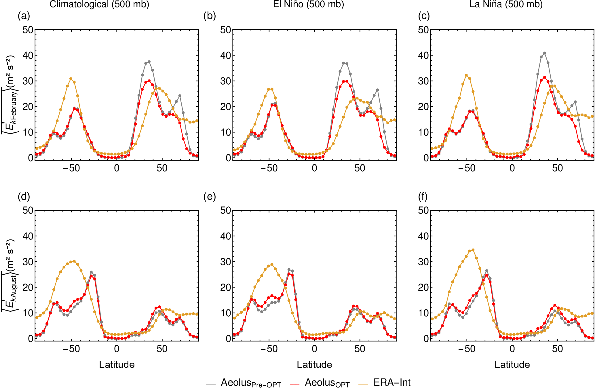
Figure 7 shows the zonal-mean eddy kinetic energy $\stackrel{\mathrm{‾}}{\langle E_k^{\prime }\rangle }$. We show the same color code as in Fig. 6. Northern Hemisphere modeled $\stackrel{\mathrm{‾}}{\langle E_k^{\prime }\rangle }$ profile is again well resolved in both seasons and for El Niño and La Niña months with the parameter optimization. Smaller spikes vanish such that the modeled $\stackrel{\mathrm{‾}}{\langle E_k^{\prime }\rangle }$ better matches the observed data. The parameter optimization gained more improvement in the Northern Hemisphere (NH) than in the Southern Hemisphere (SH).

In Figs. 8 and 9, the eddy kinetic energies $\langle E_K^{\prime }\rangle$ for February and August are displayed. The left column shows observational data and the right column model data. The top row presents climatological monthly averages, the middle row El Niño months and the bottom row La Niña months.

Figure 8Eddy kinetic energy $\stackrel{\mathrm{‾}}{\langle E_k^{\prime }\rangle }$ in February at 500 mb (compare Fig. 1).

Download

Figure 9Eddy kinetic energy $\stackrel{\mathrm{‾}}{\langle E_k^{\prime }\rangle }$ in August at 500 mb (compare Fig. 1).

Download

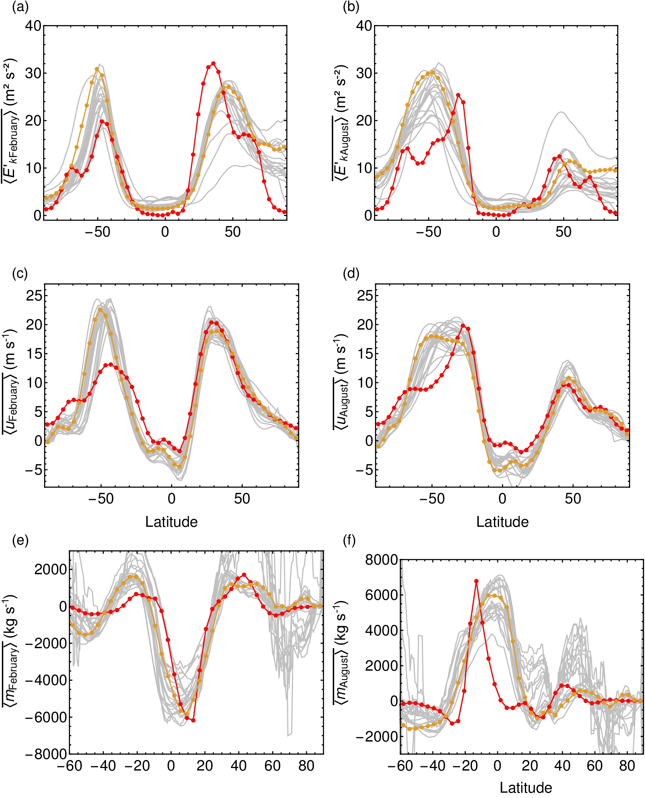
Figure 10Comparison to CMIP5 models. The orange line represents ERA-Interim data, the red line results from Aeolus and gray lines CMIP5 models (annual mean zonal-mean data).

Download

The spatial position and the magnitude are well captured; seasons and the ENSO cycles are also well resolved, with some discrepancies in the tropics (i.e., the region over the Atlantic and Pacific oceans) and the Southern Hemisphere. In February and August, $\langle E_K^{\prime }\rangle$ is stronger in the Northern Hemisphere than in the Southern Hemisphere for both the climatology and in El Niño months. Only in La Niña months, $\langle E_K^{\prime }\rangle$ is weaker in the Northern Hemisphere.

The optimized parameters are listed in Table 3. The parameters U₀ and m for optimizing the eddy kinetic energy are greater than the manually tuned values.

The parameters d₃ and n₃ are close to 1, whereas the parameters d₂, d₄ and n₁ are close to 2 and have a strong impact on the amplitude of the Hadley cell and the Ferrell cell. The parameter with the smallest influence is d₁.

6.3 Comparison to CMIP5 models

Figure 10 shows the comparison of February and August $\stackrel{\mathrm{‾}}{\langle E_k^{\prime }\rangle },\stackrel{\mathrm{‾}}{\langle u\rangle }$ and $\stackrel{\mathrm{‾}}{\langle m\rangle }$ between CMIP5 models (gray lines), Aeolus (red) and ERA-Interim data (orange). In general, CMIP5 models represent the $\stackrel{\mathrm{‾}}{\langle E_k^{\prime }\rangle }$ and $\stackrel{\mathrm{‾}}{\langle u\rangle }$ very well in both hemispheres. However, in the Southern Hemisphere, the storm tracks, i.e., $\stackrel{\mathrm{‾}}{\langle E_k^{\prime }\rangle }$, of all models are too weak compared to observations with Aeolus on the lower end of the CMIP5 range. Further, some individual CMIP5 models can have too-low or too-high $\stackrel{\mathrm{‾}}{\langle E_k^{\prime }\rangle }$ and $\stackrel{\mathrm{‾}}{\langle u\rangle }$ compared to ERA-Interim, similar to Aeolus.

The CMIP5 multimodel mean of $\stackrel{\mathrm{‾}}{\langle m\rangle }$ appears to be close to the reanalysis and most models reproduce this well. Still, some CMIP5 models can differ strongly from $\stackrel{\mathrm{‾}}{\langle m\rangle }$ in ERA-Interim with some spiky behavior. Nevertheless, the width and strength of the Hadley cell is in most models well presented, but the Ferrell cell is often too strong. Aeolus' results give reasonable strength and width of the Ferrell cell, but the width of the Southern Hemisphere Hadley cell in August is too small compared to both reanalysis and CMIP5 models.