the Creative Commons Attribution 4.0 License.
the Creative Commons Attribution 4.0 License.
 | 16 Mar 2018
Global high-resolution simulations of tropospheric nitrogen dioxide using CHASER V4.0
Kazuyuki Miyazaki
Koji Ogochi
Kengo Sudo
Masayuki Takigawa
We evaluate global tropospheric nitrogen dioxide (NO2) simulations using the CHASER V4.0 global chemical transport model (CTM) at horizontal resolutions of 0.56, 1.1, and 2.8∘. Model evaluation was conducted using satellite tropospheric NO2 retrievals from the Ozone Monitoring Instrument (OMI) and the Global Ozone Monitoring Experiment-2 (GOME-2) and aircraft observations from the 2014 Front Range Air Pollution and Photochemistry Experiment (FRAPPÉ). Agreement against satellite retrievals improved greatly at 1.1 and 0.56∘ resolutions (compared to 2.8∘ resolution) over polluted and biomass burning regions. The 1.1∘ simulation generally captured the regional distribution of the tropospheric NO2 column well, whereas 0.56∘ resolution was necessary to improve the model performance over areas with strong local sources, with mean bias reductions of 67 % over Beijing and 73 % over San Francisco in summer. Validation using aircraft observations indicated that high-resolution simulations reduced negative NO2 biases below 700 hPa over the Denver metropolitan area. These improvements in high-resolution simulations were attributable to (1) closer spatial representativeness between simulations and observations and (2) better representation of large-scale concentration fields (i.e., at 2.8∘) through the consideration of small-scale processes. Model evaluations conducted at 0.5 and 2.8∘ bin grids indicated that the contributions of both these processes were comparable over most polluted regions, whereas the latter effect (2) made a larger contribution over eastern China and biomass burning areas. The evaluations presented in this paper demonstrate the potential of using a high-resolution global CTM for studying megacity-scale air pollutants across the entire globe, potentially also contributing to global satellite retrievals and chemical data assimilation.


Nitrogen oxides (NOx ≅ NO+NO2) play a key role in air quality, tropospheric chemistry, ecosystem, and climate change. NOx is one of the main precursors of tropospheric ozone, a major pollutant and greenhouse gas (IPCC, 2013). Oxidation products from NOx, including nitric acid (HNO3), alkyl nitrates (RONO2), and peroxynitrates (RO2NO2), are partitioned to particulate nitrates, which cause respiratory problems, degrade visibility, and affect the radiative budget by scattering solar radiation. The wet and dry deposition of nitrogen compounds affects the productivities and diversities of terrestrial and marine ecosystems on a global scale (e.g., Gruber and Galloway, 2008; Duce et al., 2008). Increasing NOx also reduces quantities of long-lived greenhouse gases, such as methane, due to chemical destruction via hydroxyl radicals (OH) through O3–HOx–NOx chemistry (e.g., Shindell et al., 2009).
Major anthropogenic sources of NOx are ground transport and power generation, with these accounting for more than half of total global anthropogenic emissions (Janssens-Maenhout et al., 2015). NOx is also emitted from natural sources: biomass burning, microbial activity in soil, and lightning. Main NOx sinks are oxidation with OH during daytime and the hydrolysis of dinitrogen pentoxide (N2O5) on aerosols during nighttime (Platt et al., 1984; Dentener and Crutzen, 1993; Evans and Jacob, 2005; Brown et al., 2006). The lifetime of NOx, which is a function of OH concentration and NO2 photolysis during daytime (Prather and Ehhalt, 2001), is of the order of hours to days. It also depends on aerosol surface area and composition during nighttime (e.g., Brown et al., 2006). Because of this short lifetime and heterogeneous source distribution, tropospheric NOx is highly variable in space and time over the globe.
Satellite observations of tropospheric NO2 columns from the Global Ozone Monitoring Experiment (GOME), the SCanning Imaging Absorption SpectroMeter for Atmospheric CHartographY (SCIAMACHY), the Ozone Monitoring Instrument (OMI) (e.g., Duncan et al., 2016; Krotkov et al., 2016), and GOME-2 (e.g., Valks et al., 2011; Zien et al., 2014) have been used for evaluations of chemical transport models (CTMs) (e.g., Kim et al., 2009; Huijnen et al., 2010a; Miyazaki et al., 2012; Yamaji et al., 2014). Previous model validation studies have revealed a general underestimation of simulated tropospheric NO2 columns over polluted areas in global CTMs (van Noije et al., 2006; Huijnen et al., 2010a, b; Miyazaki et al., 2012). Global CTMs typically have a horizontal resolution of 2–5∘. Meanwhile, high-resolution simulations have been conducted using regional models, which have shown the ability to simulate observed high tropospheric NO2 columns over major polluted regions such as East Asia, North America, and Europe (e.g., Uno et al., 2007; Kim et al., 2009; Huijnen et al., 2010a; Itahashi et al., 2014; Yamaji et al., 2014; Canty et al., 2015; Han et al., 2015; Harkey et al., 2015). High-resolution simulations can lead to improvements in two ways: (1) through reduced spatial representation gaps between observed and simulated fields and (2) via improved representation of large-scale concentration fields through a consideration of small-scale processes. Using a regional CTM, Valin et al. (2011) suggested that insufficient model resolution leads to enhanced OH, shortened NO2 lifetime, and too-low NO2 over strong local emissions. The authors also suggested that 4 and 12 km resolutions are sufficient to accurately simulate the nonlinear effects of O3–HOx–NOx chemistry on NO2 lifetime over power plants in Four Corners–San Juan and Los Angeles. Yamaji et al. (2014) estimated up to 60 % error reduction in simulated tropospheric NO2 columns at 20 km resolution over East Asia compared to 80 km resolution. Using a global CTM, Wild and Prather (2006) reported that NOx lifetime over East Asia increased by 22 % when increasing model resolution from 5.6∘ × 5.6∘ to 1.1∘ × 1.1∘. Williams et al. (2017) conducted a comprehensive evaluation of NO2, SO2, and CH2O simulated in TM5-MP, revealing that increasing horizontal model resolution from 3∘ × 2∘ to 1∘ × 1∘ reduced negative NO2 bias by up to 99 % against 35 % of the surface measurement sites (33 stations) in Europe. Horizontal model resolution could also be a crucial factor even for biomass burning areas because of highly varying emission sources and nonlinear chemical processes. However, previous studies have mostly focused on urban regions. Further investigations are required for both urban and biomass burning regions. Vertical model resolution could also be important through, for instance, vertical mixing between planetary boundary layers and the free troposphere (e.g., Menut et al., 2013).
Simulated global NO2 fields provide important information on satellite retrieval and data assimilation, as well as contributing to a better understanding of the atmospheric environment (e.g., Boersma et al., 2011; Valks et al., 2011; Miyazaki et al., 2012; Williams et al., 2017). The quality of a priori fields is important for retrieval of the tropospheric NO2 column (Russell et al., 2011). For instance, low-resolution global CTMs poorly represent NO2 variations across urban and rural regions, degrading the spatial variation of retrieved concentrations at high resolution. Several retrieval studies (Heckel et al., 2011; Russell et al., 2011; Lin et al., 2014) have employed high-resolution a priori fields from regional CTM simulations. The authors demonstrated improvements in these regional retrievals using high-resolution a priori fields in comparison to the ARCTRAS aircraft observation and ground-based remote sensing MAX-DOAS through, for instance, clearer separation of NO2 profiles between urban, rural, and ocean regions and improved representations of altitude-dependent sensitivities (i.e., averaging kernels).
Global chemical data assimilation (e.g., Inness et al., 2015; Miyazaki et al., 2015) and emission inversion (e.g., Stavrakou et al., 2013; Miyazaki et al., 2017) would also benefit from high-resolution global CTMs through improvements in model performance (e.g., Arellano Jr. et al., 2007) and reduced spatial representation gaps between observed and simulated fields. Several previous studies (Mijling and van der A, 2012; Ding et al., 2017b; Liu et al., 2017) demonstrated the importance of high-resolution modeling in detecting small-scale NOx emission sources such as urban, new power plant, and ship emissions. A systematic evaluation of high-resolution models enables us to discuss the application potentials of global high-resolution models to satellite retrievals and data assimilation.
In this study, we conduct a systematic evaluation of global high-resolution simulations of tropospheric NO2 and related chemistry using CHASER V4.0. We focus on the impacts of horizontal model resolution on global tropospheric NO2 simulations. Three horizontal resolutions of 2.8, 1.1, and 0.56∘ are evaluated using satellite and aircraft measurements. The remainder of this paper is structured as follows. Section 2 describes the model configuration and simulation settings and optimizes the simulated meteorological fields at different horizontal resolutions. Section 2.2 describes the observations used for validations. Section 4 presents the model evaluation results of tropospheric NO2 using satellite-derived retrievals for the year 2008 and aircraft campaign observations from the 2014 Front Range Air Pollution and Photochemistry Experiment (FRAPPÉ). Section 5 discusses the resolution dependence of tropospheric chemistry. In Sect. 6, we then discuss the implications of this evaluation and the potential benefits of applying global high-resolution CTMs. Finally, Sect. 7 provides concluding remarks.
2.1 CHASER V4.0 model and simulations
CHASER V4.0 (Sudo et al., 2002; Sudo and Akimoto, 2007; Sekiya and Sudo, 2014) is a global chemical transport model developed in the framework of the MIROC-ESM Earth system model (Watanabe et al., 2011), which is coupled online with the MIROC-AGCM atmospheric general circulation model (AGCM) (K-1 model developers, 2004) and the SPRINTARS aerosol transport model (Takemura et al., 2005, 2009). Several updates were made from CHASER V3.0 (Sudo et al., 2002) to CHASER V4.0, which includes the consideration of aerosol species (sulfate, nitrate, ammonium, black and organic carbon, soil dust, and sea salt) and the implementation of related chemistry, radiation, and cloud processes. AGCM was also updated from the NIES/CCSR AGCM 5.7b to the MIROC-AGCM. Detailed information on the AGCM updates are provided by K-1 model developers (2004).
CHASER calculates gaseous, aqueous, and heterogeneous chemical reactions (93 species and 263 reactions), including the O3–HOx–NOx–CH4–CO system with the oxidation of non-methane volatile organic compounds (NMVOCs). Major chemical reactions related to NO2 are considered, including (1) the photochemical cycle of NO and NO2, (2) oxidation of NO2 with OH, (3) heterogeneous hydrolysis of N2O5, (4) the formation, thermal decomposition, and photolysis of peroxyacetyl nitrates (PANs), and (5) the formation of isoprene nitrates. CHASER also calculates stratospheric O3 chemistry including Chapman mechanisms and catalytic reactions related to HOx, NOx, ClOx, and BrOx below 50 hPa. Above 50 hPa, prescribed concentrations of O3, nitrogen, and halogen species are used. Monthly ozone climatology is obtained from UGAMP (Li and Shine, 1995), whereas monthly climatologies of nitrogen and halogen species are taken from the Chemistry–Climate Model Initiative (CCMI) REF-C1SD simulation using NIES CCM (Akiyoshi et al., 2009, 2016; Morgenstern et al., 2016). Dry and wet (rain out and washout) deposition is calculated based on the resistance-based parameterization (Wesely, 1989) and cumulus convection and large-scale condensation parameterizations, respectively. Advective tracer transport is calculated using the piecewise parabolic method (Colella and Woodward, 1984) and the flux-form semi-Lagrangian scheme (Lin and Rood, 1996). The model also incorporates tracer transport on a sub-grid scale in the framework of the prognostic Arakawa–Schubert cumulus convection scheme (Emori et al., 2001) and the vertical diffusion scheme (Mellor and Yamada, 1974).
We evaluated two 1-year global simulations for tropospheric NO2 in 2008 and 2014 with a 1-year spin-up calculation for each simulation. In each case, three model calculations were conducted at different horizontal resolutions: T42 (i.e., 2.8∘ × 2.8∘; hereinafter referred to as the 2.8∘ simulation), T106 (i.e., 1.1∘ × 1.1∘; hereinafter the 1.1∘ simulation), and T213 (i.e., 0.56∘ × 0.56∘; hereinafter the 0.56∘ simulation); 32 vertical layers from the surface to approximately 40 km altitude were used across the three simulations. To meet the Courant–Friedrich–Levy (CFL) condition, different maximal time steps were used for each resolution: i.e., 20 min at 2.8∘ resolution, 8 min at 1.1∘ resolution, and 4 min at 0.56∘ resolution. Sea-surface temperatures (SSTs) and sea-ice concentrations (SICs) were prescribed by HadISST for the corresponding year (Rayner et al., 2003). Simulated air temperature and horizontal wind were nudged to 12-hourly ERA-Interim reanalysis data (Dee et al., 2011). ERA-Interim reanalysis data at 0.75∘ × 0.75∘ horizontal resolution with 37 pressure levels were linearly interpolated to each model grid, possibly degrading simulated meteorological fields at finer resolution (i.e., 0.56∘). We specified 5 and 0.7 days of nudging time for temperature and horizontal wind, respectively.
NOx emissions from anthropogenic, biomass burning, lightning, and soil sources were considered. Anthropogenic emissions from the HTAP_v2.2 inventory for the year 2008 (Janssens-Maenhout et al., 2015) were employed for the 2008 simulations, with these originally having 0.1∘ × 0.1∘ resolution. For the 2014 simulation, anthropogenic emissions for the latest available year 2010 of the HTAP_v2.2 inventory were used. Biomass burning emissions were taken from the Global Fire Emissions Database (GFED) version 4.1 (0.25∘ × 0.25∘ resolution) (Giglio et al., 2013) for the two study years. Soil emissions were obtained from the Global Emission InitiAtive (GEIA) database (1∘ × 1∘) (Yienger and Levy, 1995). Model of Emissions of Gases and Aerosols from Nature (MEGAN) version 2 data (0.5∘ × 0.5∘) were used for biogenic NMVOCs emissions (Guenther et al., 2006). Annual mean total global NOx emissions from the surface were 45.3 and 45.9 Tg N yr−1 in 2008 and 2014, respectively. Lightning NOx sources were calculated as a function of cloud top height in the cumulus convection parameterization (prognostic Arakawa–Schubert scheme) at each time step of CHASER, following Price and Rind (1992).
We considered diurnal cycles of surface NOx emissions following Miyazaki et al. (2012). Different diurnal cycles were assumed depending on the dominant source category of each region: anthropogenic-type diurnal cycles (with maxima in the morning and evening, with a factor of about 1.4) over Europe, eastern China, Japan, and North America; biomass-burning-type diurnal cycles (with a rapid increase in the morning and maximum midday, with a factor of about 3) over Central Africa and South America; and soil-type diurnal cycles (with maxima in the afternoon, with a factor of about 1.2) in the grasslands or sparsely vegetated areas of Australia, Sahara, and western China. Miyazaki et al. (2012) confirmed that the application of this scheme leads to improvements in global tropospheric NO2 simulations at 2.8∘ resolution. Improvements were commonly found in the 1.1∘ resolution simulation, whereas we did not evaluate the impact at 0.56∘ resolution. Over biomass burning regions, the emission diurnal variability applied in this study is generally similar to variability from 3-hourly GFED4.1 data, while distinct differences in relative magnitude around the GOME-2 overpass time suggest that model performance could differ in comparison to the GOME-2 retrievals when using the 3-hourly GFED4.1 data.
The CTM–AGCM online coupling framework used in this study has advantages over the off-line CTM framework driven by meteorological analysis or reanalysis data. First, the online framework is able to simulate short-term nonlinear variations in chemical and transport processes at every time step of the model (1–20 min in this study) in contrast to off-line CTMs driven by meteorological data, typically with 6-hourly intervals. Second, grid-scale and sub-grid-scale transport processes (e.g., convection, turbulent mixing) are represented in a consistent manner based on AGCM physics (e.g., mass balance) at short time intervals. Third, the online framework allows for a flexible choice of CTM resolution, whereas the off-line framework requires matching (or interpolations without physically meaningful variations) between the CTM and meteorological data resolutions.
2.2 Observations
2.2.1 Satellite tropospheric NO2 retrievals
We used tropospheric NO2 column retrievals from OMI and GOME-2. OMI, onboard the Aura satellite, is an ultraviolet–visible nadir-scanning solar-backscatter spectrometer covering the spectral range of 270–500 nm (Levelt et al., 2006). The Aura satellite, launched in 2004, is in a Sun-synchronous polar orbit at 705 km of altitude with a local Equator crossing time of approximately 13:40 LT. The ground pixel size of OMI ranges from 13 × 24 km2 to 26 × 128 km2 depending on the satellite viewing angle. OMI tropospheric NO2 column retrievals have daily global coverage. We used the DOMINO version 2.0 data product (Boersma et al., 2011) obtained from the TEMIS website (http://www.temis.nl/). Observations with cloud radiance fraction < 0.5, surface albedo < 0.3, and quality flag 0 were used. Retrievals from 2014 affected by row anomalies were screened using a quality flag.
Tropospheric NO2 retrievals from GOME-2 on MetOP-A and MetOP-B were used to compare the years 2008 and 2014, respectively. GOME-2 is a nadir-scanning ultraviolet–visible spectrometer covering the spectral range of 240–790 nm. MetOp-A, launched in 2007, and MetOp-B, launched in 2013, are on a Sun-synchronous polar orbit at 817 km with a local Equator crossing time of 09:30 LT. The ground pixel size is 80 × 40 km2. We used the TM4NO2A version 2.3 product obtained from the TEMIS website (Boersma et al., 2004). The GOME-2 retrievals were derived with the same basic algorithm as in DOMINO version 2 (Boersma et al., 2011).
For model–retrieval comparisons, we first sampled simulated NO2 profiles at the closest times to measurement using 2-hourly model outputs; these were then linearly interpolated to the center of each measurement from the four surrounding model grids. Second, averaging kernels (AKs) were applied to the interpolated model profiles in order to consider the altitude-dependent sensitivity of retrievals. Third, retrieved and simulated NO2 columns were averaged on 0.5 and 2.8∘ bin grids for model evaluation. In order to identify the drivers of model–retrieval differences and causes of NO2 error reductions in high-resolution simulations, we conducted model evaluations at 0.5 and 2.8∘ bin grids (i.e., the model and retrieval fields were interpolated to 0.5 and 2.8∘ bin grids). Improved agreement in high-resolution simulations can be attributed to two factors: (1) closer spatial representativeness between simulations and satellite retrievals (up to approximately 0.5∘) and (2) improvements in mean concentration fields on a large scale (i.e., at 2.8∘) through the consideration of small-scale processes. The error reductions evaluated at the 0.5∘ bin grid should reflect both effects, whereas error reductions evaluated at the 2.8∘ bin grid should mainly be attributed to the latter effect (2). When error reductions evaluated at the 2.8∘ bin grid are about half the error reductions evaluated at the 0.5∘ bin grid, the contributions of the two effects should be identical. When error reductions evaluated at 2.8 and 0.5∘ bin grids are comparable, the latter effect (2) should be dominant.
It should be noted that tropospheric NO2 retrievals from SCIAMACHY were also available for 2008. The model evaluation results are generally similar between GOME-2 and SCIAMACHY. Results using SCIAMACHY are not discussed in this paper.
2.2.2 Aircraft observation data
Vertical profiles of NO, NO2, OH, HO2, O3, H2O, and the photolysis rate of O3 to O(1D) were obtained from the 2014 Front Range Air Pollution and Photochemistry Experiment (FRAPPÉ) campaign (Vu et al., 2016). The FRAPPÉ campaign was conducted using the NSF/NCAR C130 aircraft during the period from 16 July through 18 August 2014. The C130 flight track covered the northern Colorado plains and foothills and the area west of the Continental Divide. NO, NO2, and O3 concentrations were measured by two-channel (for NO and NO2) and one-channel (for O3) chemiluminescence instruments (Ridley et al., 2004). OH and HO2 were analyzed using a CIMS-based instrument that is part of the Mauldin–Cantrell HOx CIMS instrument (e.g., Mauldin et al., 2003). Water vapor was measured by a wavelength-scanned cavity ring-down spectroscopy (WS-CRDS) analyzer. The photolysis rate of O3 to O(1D) data, calculated from NCAR HARP–CFAS (CCD-based actinic flux spectroradiometer), were used. We used 1 min merged data obtained from the NASA LaRC Airborne Science Data for Atmospheric Composition (http://www-air.larc.nasa.gov/). For comparison purposes, we sampled simulated profiles at the closest time to measurement using 2-hourly model outputs; these were then linearly interpolated to measurement from the four surrounding model grids in the horizontal. The observed and simulated vertical profiles were compared by averaging data within each vertical pressure bin: 850 hPa (using data between the surface and 825 hPa), 800 hPa (825–775 hPa), 750 hPa (775–725 hPa), 700 hPa (725–675 hPa), 650 hPa (675–625 hPa), 600 hPa (625–575 hPa), 550 hPa (575–525 hPa), and 500 hPa (525–475 hPa).
2.2.3 Ozonesonde
Simulated vertical profiles of tropospheric ozone were also evaluated using ozonesonde observations. The observed vertical profiles of ozone were obtained from the World Ozone and Ultraviolet Data Center (WOUDC, https://woudc.org/), the Southern Hemisphere ADditional OZonesondes (SHADOZ, https://tropo.gsfc.nasa.gov/shadoz/) (Thompson et al., 2003a, b), and the NOAA Earth System Research Laboratory (ESRL) Global Monitoring Division (GMD, https://www.esrl.noaa.gov/gmd/). All available data from these sources were used. The observed and simulated ozone profiles were compared at ozonesonde locations by averaging data within each vertical pressure bin: 850 hPa (875–825 hPa), 500 hPa (550–450 hPa), 300 hPa (350–275 hPa), and 100 hPa (112.5–92.5 hPa).
In the CTM-AGCM online framework, meteorological fields vary among different model resolutions. From sensitivity calculations, the strength and distribution of the cumulus convection were found to be sensitive to model resolution. The cumulus convection parameterization for 2.8∘ resolution was optimized following Watanabe et al. (2011). We then attempted to optimize the relevant model parameters (critical relative humidity for cumulus convection and ice-fall speed) for 1.1 and 0.56∘ resolutions. The criterion was to minimize the root mean square error (RMSE) of annual global total flash against the Lightning Imaging Sensor (LIS), outgoing longwave radiation (OLR) against the NOAA 18 satellite observations (Liebmann, 1996), and precipitation against the Global Precipitation Climatology Project (GPCP) (Adler et al., 2003; Huffman et al., 2009) for the year 2008. The obtained minimum values of RMSE for annual mean flash rate were 0.010, 0.011, and 0.011 flashes km−2 day−1 at 2.8, 1.1, and 0.56∘ resolutions, respectively. Optimizing the cumulus convection setting reduced the positive bias of the annual global mean OLR by 80 % at 1.1∘ resolution and by 50 % at 0.56∘ resolution. Simulated global flash frequency and annual global lightning NOx sources (in brackets) varied slightly: 43 flashes s−1 (5.4 Tg N yr−1) at 2.8∘ resolution, 47 flashes s−1 (5.6 Tg N yr−1) at 1.1∘ resolution, and 46 flashes s−1 (5.5 Tg N yr−1) at 0.56∘ resolution.
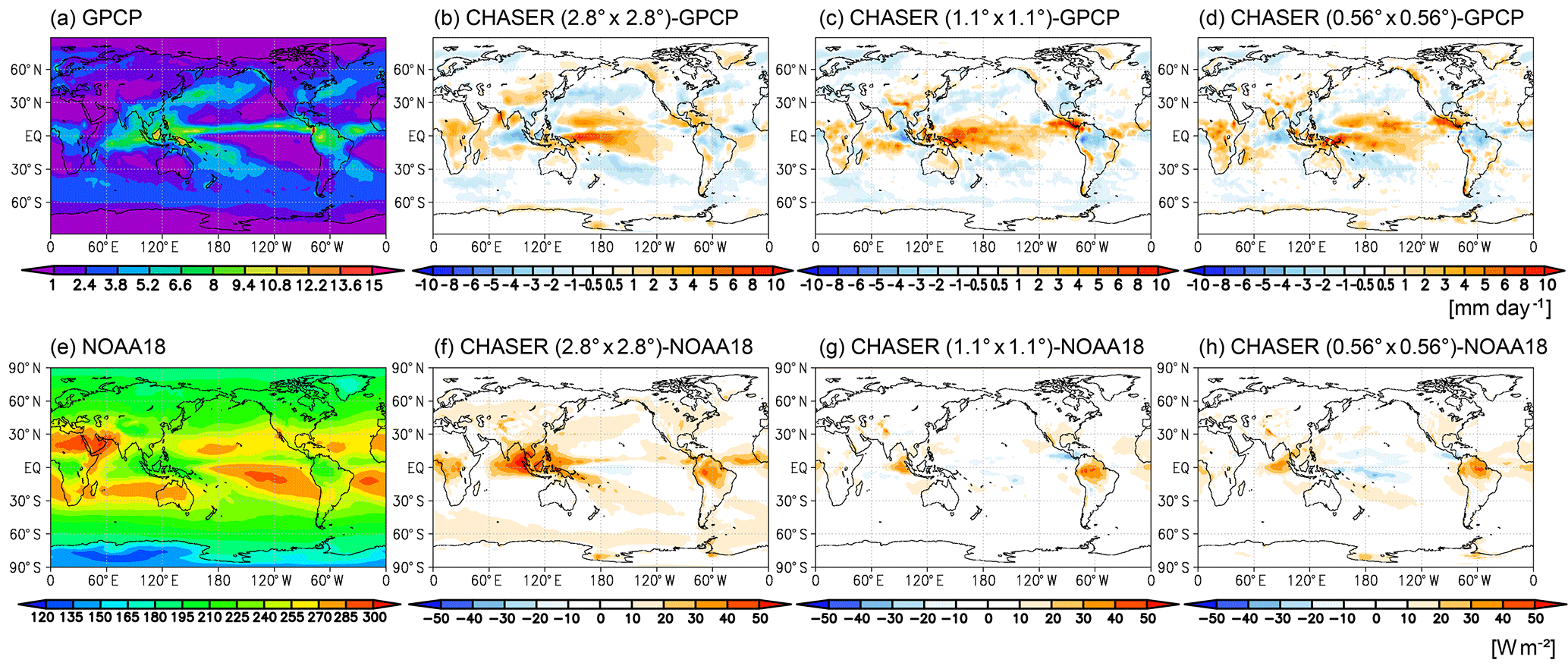
Figure 1Annual mean precipitation rate (mm day−1) from GPCP (a) and outgoing longwave radiation (OLR; W m−2) from NOAA 18 satellite (e) for 2008. The second, third, and fourth columns show differences in precipitation (b–d) and OLR (f–h) between the observations and the model simulations at 2.8∘ (b, f), 1.1∘ (c, g), and 0.56∘ (d, h) resolutions, respectively. The observations and model results are mapped onto 2.5 and 1∘ bin grids for precipitation and OLR, respectively.

Figure 2Annual mean tropospheric NO2 column (× 1015 molecules cm−2) from satellite retrievals (first column; a, e) and differences between the model simulation at 2.8∘ (second column; b, f), 1.1∘ (third column; c,g), and 0.56∘ (fourth column; d, h) resolutions and satellite retrievals from OMI (upper row; a–d) and GOME-2 (lower row; e–h) for 2008. The observed and simulated fields are mapped onto a 0.5∘ bin grid. The white square line in (a) represents the region used for the model evaluation.
We also evaluated relevant meteorological fields (i.e., precipitation and cloud) that have large impacts on chemistry simulations in the online CTM framework (e.g., Hess and Vukicevic, 2003). In comparison to the GPCP precipitation data, all simulations showed similar spatial error patterns after optimization (Fig. 1a–d), having positive biases (typically by a factor of 2) north and south of the intertropical convergence zone (ITCZ) over the Pacific, Indian subcontinent, and Central Africa and negative biases in the South Pacific convergence zone (SPCZ), west of the Maritime Continent, over the Amazon, and over the southeastern United States because of the use of the same physical package (e.g., cumulus convection scheme). Meanwhile, increasing model resolution led to large error reductions by up to 70 % at 1.1 and 0.56∘ resolutions over the northwest Pacific and Atlantic oceans (negative biases) and over the northern part of China and the western part of the North American continent (positive biases). All simulations also showed reasonable agreement with OLR derived from the NOAA 18 satellite. The global mean positive bias was 80 and 50 % lower at 1.1 and 0.56∘ resolutions, respectively, than at 2.8∘ resolution (Fig. 1e–h), suggesting improved photolysis calculations in the high-resolution simulations. Among different regions, the positive model bias at 2.8∘ resolution was largest over the Maritime Continent, which was reduced by 86 % at 1.1∘ resolution and by 75 % at 0.56∘ resolution. Over northern South America, in contrast, most of the positive biases remained at 1.1 and 0.56∘ resolutions. The model simulations were thus appropriately set up at all resolutions, while various features of the high-resolution framework were improved. Further validation at various spatial–temporal scales for different meteorological parameters will be helpful to evaluate detailed AGCM performance, even if it is beyond the scope of the current study.
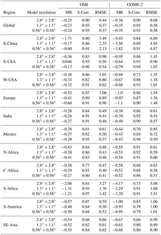
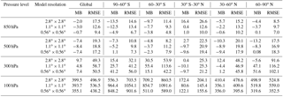
Table 1Comparisons of annual mean tropospheric NO2 column between satellite retrievals (OMI and GOME-2) and the model simulation at 2.8, 1.1, and 0.56∘ resolutions. MB is the mean bias. RMSE is the root mean square error. S-Corr. signifies the spatial correlation coefficient. Units of MB and RMSE are × 1015 molecules cm−2. The definition of the regions is the same as in Fig. 3.
4.1 Global and regional distributions
Figure 2 compares the simulated annual mean tropospheric NO2 column with satellite retrievals. Both OMI and GOME-2 retrievals showed high tropospheric NO2 columns over eastern China, the United States, Europe, India, Southeast Asia, Central and South Africa, and South America. For most of these regions, observed concentrations were higher in GOME-2 than OMI, reflecting the difference in overpass time and diurnal variations in tropospheric chemistry (Boersma et al., 2008). All model simulations captured the observed global spatial variation well, with r>0.9 in comparison to both OMI and GOME-2 for annual mean concentration fields. In terms of global averages, the 2.8∘ simulations were biased on the low side by 40 % compared to OMI and by 47 % compared to GOME-2. This negative global mean bias has commonly been reported using other global CTMs (van Noije et al., 2006; Huijnen et al., 2010b; Miyazaki et al., 2012). As summarized in Table 1, the negative annual global mean bias compared to OMI (GOME-2) was slightly reduced by 5 % (3 %) at 1.1∘ resolution and by 2 % (1 %) at 0.56∘ resolution compared to the 2.8∘ resolution. Global RMSE was reduced by 15 % compared to OMI and GOME-2 by increasing model resolution from 2.8 to 1.1∘. The improvement when increasing resolution from 1.1 to 0.56∘ was limited.
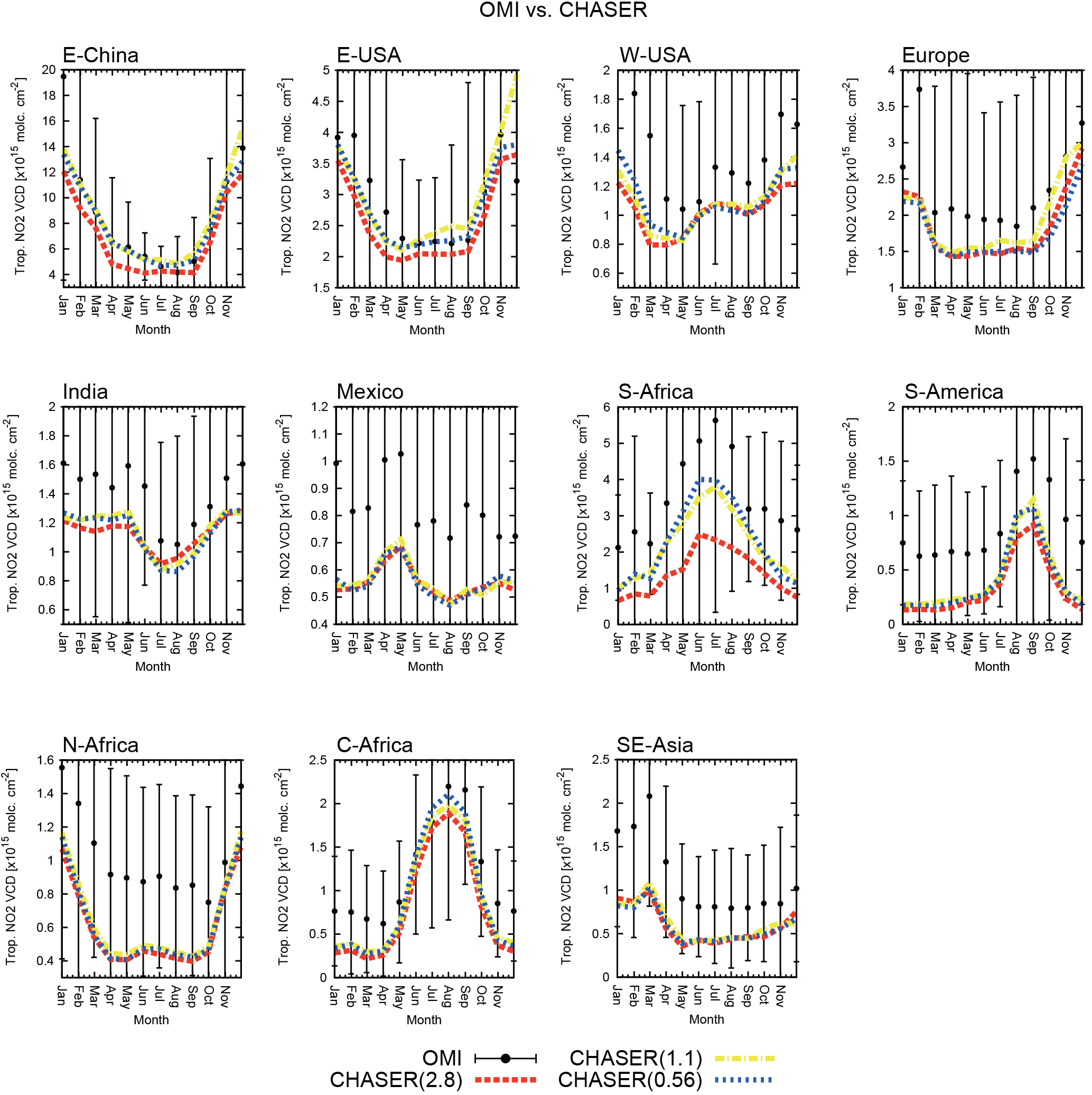
Figure 3Monthly time series of tropospheric NO2 column (× 1015 molecules cm−2) averaged in E-China (110–123∘ E, 30–40∘ N), E-USA (95–71∘ W, 32–43∘ N), W-USA (125–100∘ W, 32–43∘ N), Europe (10∘ W–30∘ E, 35–60∘ N), India (68–88∘ E, 8–35∘ N), Mexico (115–90∘ W, 15–25∘ N), N-Africa (20∘ W–40∘ E, 0–20∘ N), C-Africa (10–40∘ E, 20∘ S–0), S-Africa (26–31∘ E, 28–23∘ S), S-America (70–50∘ W, 20∘ S–0), and SE-Asia (96–105∘ E, 10–20∘ N). The black dots are OMI retrievals, the red dashed line is the model simulation at 2.8∘ resolution, the yellow dashed-dotted line is the model simulation at 1.1∘ resolution, and the blue dotted line is the model simulation at 0.56∘ resolution. The vertical bars indicate mean OMI retrieval errors.
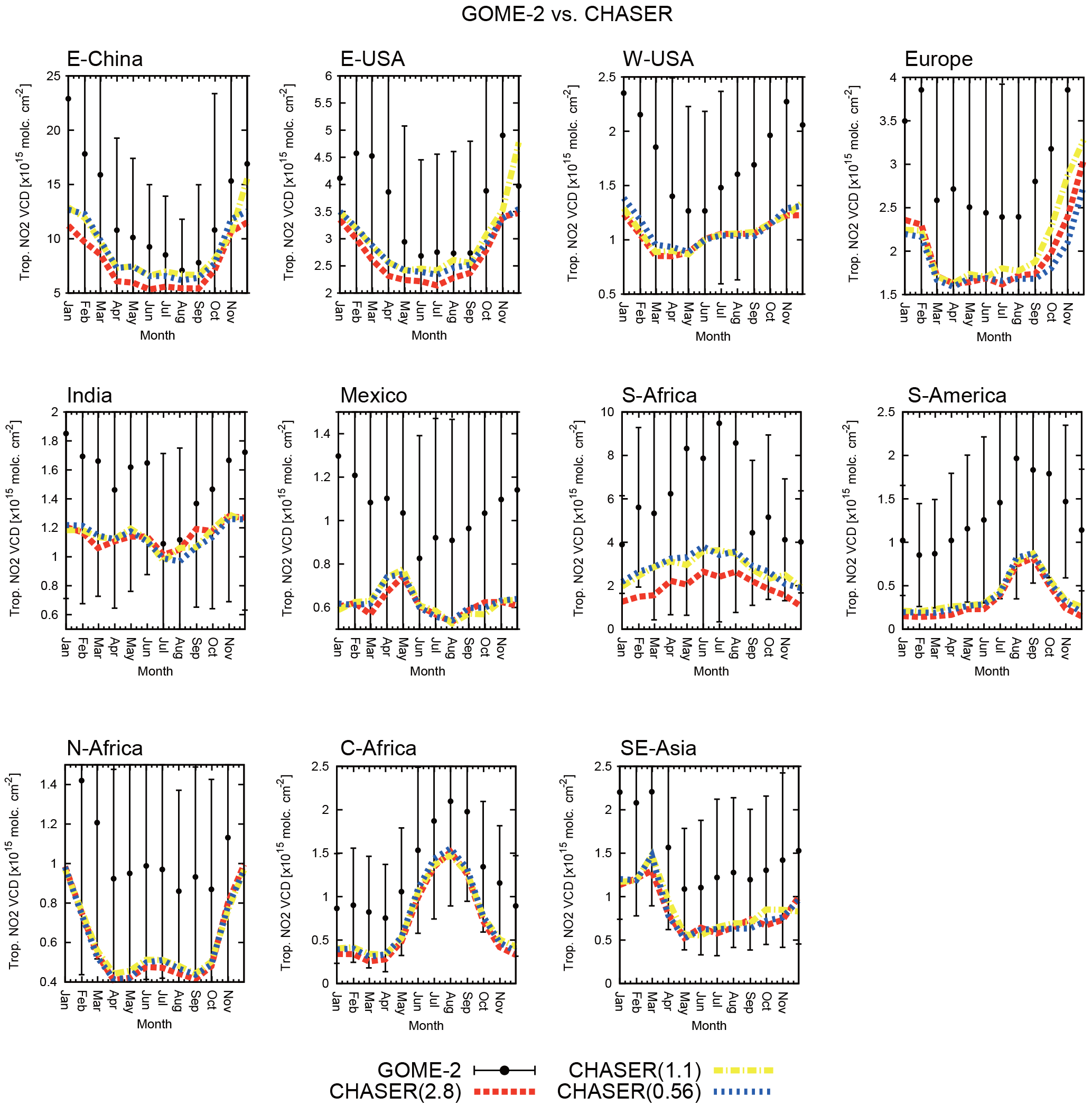
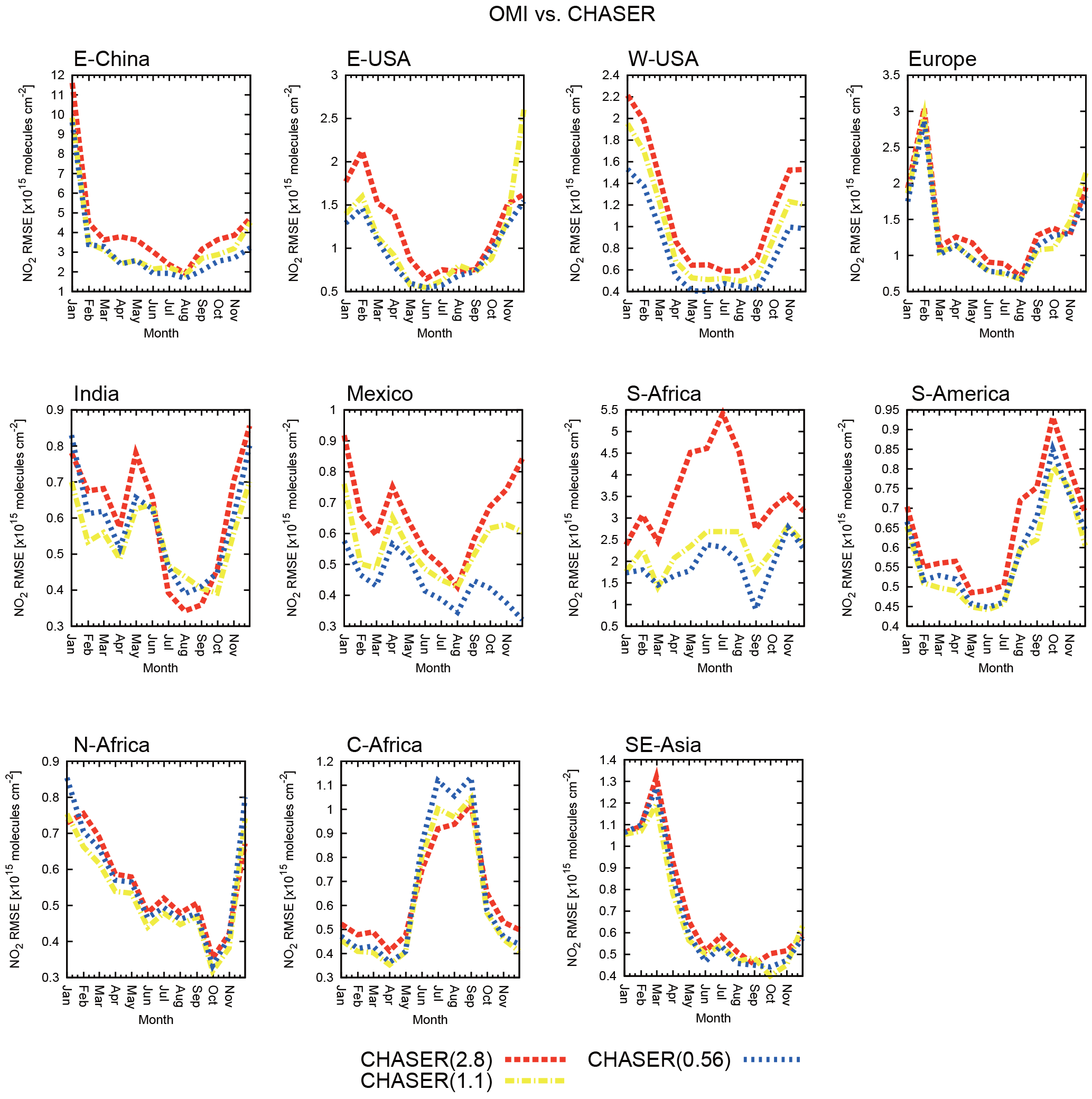
Figure 5Same as Fig. 3, but for root mean square error (RMSE) of tropospheric NO2 column in comparison to OMI.
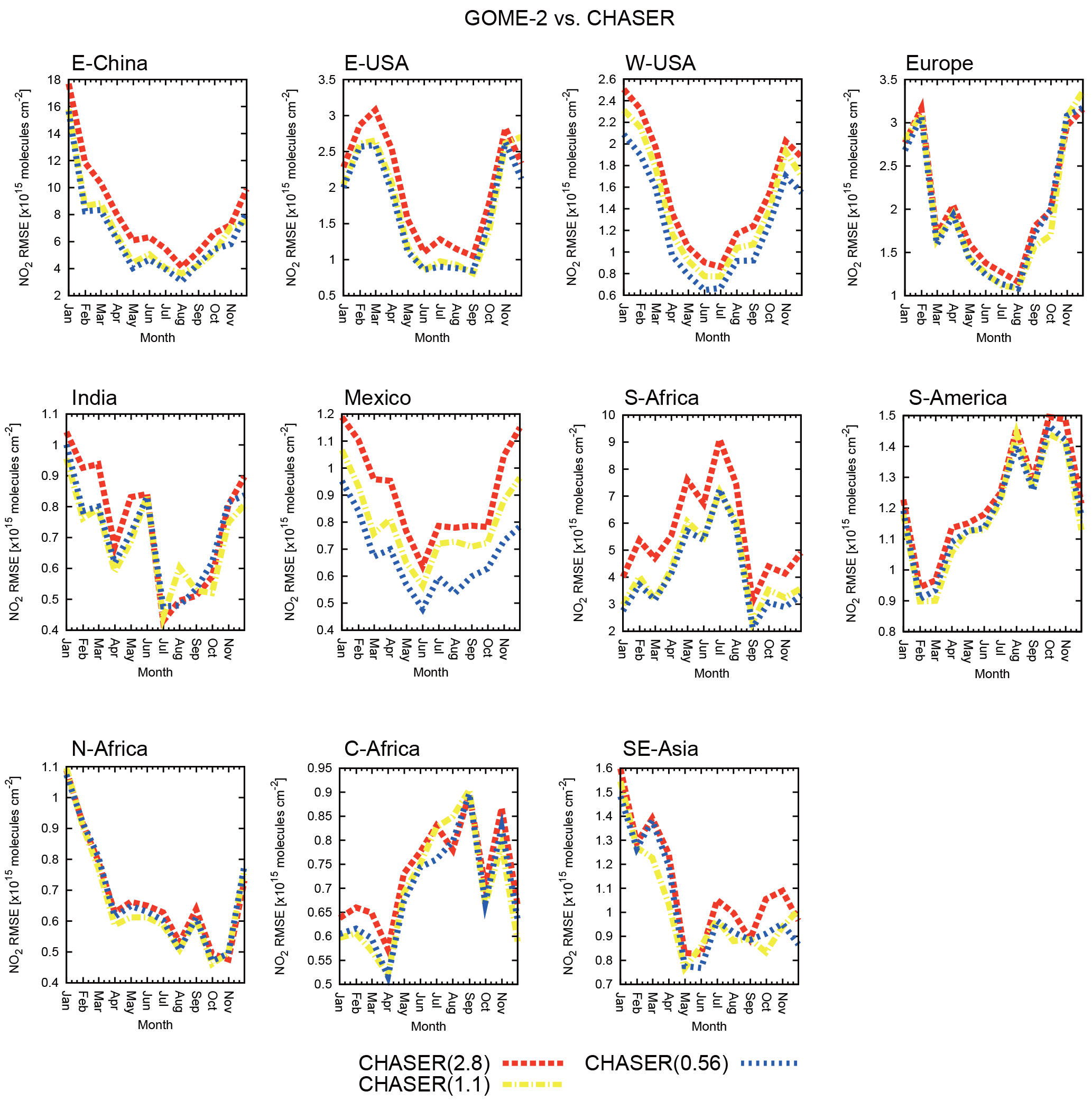
Figures 3 and 4 (5 and 6) compare seasonal variations in the regional and monthly mean tropospheric NO2 column (regional RMSEs) against OMI and GOME-2 in 2008 using data incorporated at a 0.5∘ bin grid. Because the validation results are similar for OMI and GOME-2 for most cases, the results using OMI are discussed below.
Over eastern China, negative model biases at 2.8∘ resolution were reduced at 1.1 and 0.56∘ resolutions from February to July. In December, model bias varied with model resolution: −14 % at 2.8∘ resolution, +23 % at 1.1∘ resolution, and −7 % at 0.56∘ resolution. Negative annual mean bias was reduced by 90 % from 2.8 to 1.1∘ resolution and by 64 % from 2.8 to 0.56∘ resolution, with increasing spatial correlations (from r=0.80 at 2.8∘ resolution to r=0.86 at 1.1∘ resolution and 0.91 at 0.56∘ resolution). Annual mean RMSE was also reduced by 32 % from 2.8 to 1.1∘ resolution and by 9 % from 1.1 to 0.56∘ resolution.
Over the eastern United States, negative annual mean bias was reduced by 87 % at 1.1∘ resolution and by 65 % at 0.56∘ resolution compared to 2.8∘ resolution. The seasonal bias reduction reached 95 % at 0.56∘ resolution in summer. Annual RMSE was reduced by 37 % at 1.1∘ resolution and by 40 % at 0.56∘ resolution compared to 2.8∘ resolution. The larger monthly RMSE at 1.1∘ than at 2.8∘ resolution during December is attributed to large positive biases over New Jersey and Ohio, although the reason for these is unclear. The spatial correlation for annual mean concentration fields increased from r=0.83 at 2.8∘ resolution to r=0.93 at 1.1∘ resolution and 0.96 at 0.56∘ resolution.
Over the western United States, negative annual mean bias was 13 % lower at 1.1∘ resolution and 14 % lower at 0.56∘ resolution compared to 2.8∘ resolution. In summer, the negative seasonal mean bias at 0.56∘ resolution was slightly larger, reflecting negative biases over rural areas. RMSE for annual mean fields was reduced by 20 % from 2.8 to 1.1∘ resolution and by 23 % from 1.1 to 0.56∘ resolution. The spatial correlation for annual mean fields increased from r=0.65 at 2.8∘ resolution to r=0.82 at 1.1∘ resolution and 0.91 at 0.56∘ resolution.
Over Europe, negative model bias for annual mean concentrations was reduced by 23 % from 2.8 to 1.1∘ resolution, but was 46 % larger at 0.56∘ resolution than at 1.1∘ resolution. Large negative bias over the Po Valley at 2.8∘ resolution was reduced by 13 % at 1.1∘ resolution and further reduced by 10 % from 1.1 to 0.56∘ resolution. In contrast, negative bias over London was larger at 0.56∘ resolution than at 1.1∘ resolution by a factor of 4, leading to larger negative regional mean bias at 0.56∘ resolution. Simulated planetary boundary layer (PBL) height in the 0.56∘ simulation was substantially higher (by 20 %) than ERA-Interim over London, which may partially contribute to the large NO2 bias. Annual RMSE was also lower by 16 % at 1.1∘ resolution and by 9 % at 0.56∘ resolution than at 2.8∘ resolution. The spatial correlation for annual mean fields increased from 0.87 at 2.8∘ resolution to 0.91 at 0.56∘ resolution.
Over India, negative model biases were smaller at 1.1 and 0.56∘ resolutions than at 2.8∘ resolution during January–May, but were larger during June–September. RMSE for annual mean fields was reduced at 1.1 and 0.56∘ resolutions (except during summer), with 16 and 6 % reductions, respectively. When comparing against OLR and precipitation observations, we found an increased error at 0.56∘ resolution over India during summer. This suggests the need to further optimize model parameters relevant to tropical convection (see Sect. 2) in order to improve high-resolution NO2 simulations.
Over Mexico, the spatial correlation for annual mean fields increased substantially at 1.1∘ (r=0.82) and 0.56∘ resolutions (r=0.93) compared to 2.8∘ resolution (r=0.61). Increasing model resolution was important to reduce negative biases around Mexico City, reducing annual RMSE by 17 % at 1.1∘ resolution and by 38 % at 0.56∘ resolution compared to 2.8∘ resolution.
Over South Africa, the negative annual mean bias was reduced by 37 % at 1.1∘ resolution and by 43 % at 0.56∘ resolution compared to 2.8∘ resolution, while annual RMSE was reduced by 46 and 56 % at 1.1 and 0.56∘ resolutions, respectively. The spatial correlation was 0.93 and 0.97 at 0.56∘ resolution in contrast to 0.61 at 2.8∘ resolution. Model resolution higher than 1.1∘ was thus important for reproducing megacity-scale air pollution over the Highveld region of South Africa, which is a complex source area of coal mining, thermal power generation, metal mining, and metallurgical industry as discussed by Duncan et al. (2016).
Over the selected biomass burning regions (South America, North Africa, Central Africa, and Southeast Asia), all model simulations showed negative biases throughout the year. In most cases, bias reduction with increasing model resolution was limited because most forest fires burn over large extents. Over South America, negative bias for the annual mean concentration was 15 % lower at 1.1∘ resolution and 12 % lower at 0.56∘ resolution than at 2.8∘ resolution. Annual RMSE was reduced by 15 % at 1.1∘ resolution and by 12 % at 0.56∘ resolution. The smaller spatial correlation at high resolutions reflects an increased positive bias over a major biomass burning hot spot (12∘ S, 50∘ W). Over North Africa, annual RMSE was smaller by 9 % at 1.1∘ resolution and by 3 % at 0.56∘ resolution (compared to 2.8∘ resolution), whereas changes in mean bias and spatial correlation were small. Over Central Africa, negative annual mean bias was reduced by 24 % at 1.1∘ resolution and by 30 % at 0.56∘ resolution, while RMSE increased during the biomass burning season (by 11 % at 1.1∘ resolution and by 24 % at 0.56∘ resolution). The increased RMSE is associated with increased positive biases around 10–20∘ S. Over Southeast Asia, RMSE for the annual mean fields was reduced by 7 % at 1.1∘ resolution and by 5 % at 0.56∘ resolution compared to 2.8∘ resolution. The increased errors over strong biomass burning hot spots in high-resolution simulations could be a result of more pronounced influences of largely uncertain inventories for individual burning points (e.g., Castellanos et al., 2015).
Negative biases with respect to GOME-2 were larger than to OMI in all simulations over most regions. The differences suggest that all model simulations underestimated high NO2 concentrations in the morning. The underestimations could be associated with insufficient vertical model resolution for capturing thin nocturnal boundary layers and uncertainties in HOx–NOx–CO–VOCs chemistry, NO2 photolysis rates, and emission diurnal cycles. The different model biases between OMI and GOME-2 could also be attributed to the bias between these retrievals. Irie et al. (2012) concluded that the bias between these retrievals is small and insignificant for East Asia, whereas the bias between these retrievals is unclear for other regions. For the most anthropogenically polluted regions, bias reductions at 0.56∘ (compared to 2.8∘ resolution) were similarly found for OMI and GOME-2. For South America and Central Africa, reductions of the negative bias at 0.56∘ resolution were larger in the comparison against OMI than GOME-2 during the biomass burning season, suggesting that the high-resolution simulation improves the representation of daytime photochemistry in the presence of enhanced biomass burning emissions.
For the evaluations, we used simulated and observed concentrations interpolated to a 0.5∘ bin grid. To identify the main drivers of improvements in the high-resolution simulation, we conducted further comparisons using two concentration fields interpolated to 2.8 and 0.5∘ bin grids. The drivers consist of (1) closer spatial representativeness between observations and simulations (up to approximately 0.5∘ resolution) and (2) better representation of large-scale (i.e., at 2.8∘) concentration fields through the consideration of small-scale processes. Error reductions at the 0.5∘ bin grid include the effects of both drivers. In contrast, error reductions at the 2.8∘ bin grid are mainly attributed to the latter effect (2). When error reductions at the 2.8∘ bin grid are about half those at the 0.5∘ bin grid, the contributions of the two effects should be identical. For annual RMSE reductions, the contributions of the two effects were almost identical over the eastern United States, the western United States, and South Africa (by up to −1.9 and −0.9 × 10¹⁵ molecules cm−2 at 0.5 and 2.8∘ bin grids, respectively). In contrast, over eastern China, improved representations on the large scale (2) contributed up to 90 % (i.e., reductions by 1.1 and 1.0 × 10¹⁵ molecules cm−2 at 0.5 and 2.8∘ bin grids, respectively, at 1.1∘ resolution). In this region, the large contribution of the second effect reflected spatially homogeneous error reductions over Hebei and Henan provinces. Over most biomass burning areas, improved representations on the large scale (2) dominated improvements in high-resolution modeling, with RMSE reductions of up to 0.072 × 10¹⁵ molecules cm−2 for the 2.8∘ bin grid and 0.071 × 10¹⁵ molecules cm−2 for the 0.5∘ bin grid. These results imply that, even for areas with homogeneous concentration and emission fields, high-resolution modeling can have significant impacts through a better representation of large-scale fields.
4.2 Tropospheric NO2 over strong local sources
Figure 7 compares the detailed spatial distribution of the tropospheric NO2 column in summer, as represented by OMI measurements and model simulations over four selected polluted areas: East Asia, South Asia, the western United States, and South Africa. Over East Asia, high concentrations were observed over the North China Plain, the Yangtze River Delta, the Pearl River Delta, Seoul, and Tokyo, which could mainly be attributed to emissions from traffic (Zheng et al., 2014) and large coal-fired power plants in the North China Plain (Liu et al., 2015). The 2.8∘ simulation underestimated these high concentrations and overestimated low concentrations over surrounding areas, probably associated with artificial mixing at coarse model resolution. The 1.1 and 0.56∘ simulations reduced negative biases over central eastern China, the Pearl River Delta, Seoul, Tokyo, and the western part of Japan. Over the Yellow Sea, the East China Sea, and off the Pacific coast of Japan, the positive biases at 2.8∘ resolution were mostly removed at 1.1 and 0.56∘ resolutions. Consequently, regional RMSE was 32 % lower at 0.56∘ resolution. In contrast, high-resolution simulations led to overestimation over Beijing and the Yangtze River Delta.
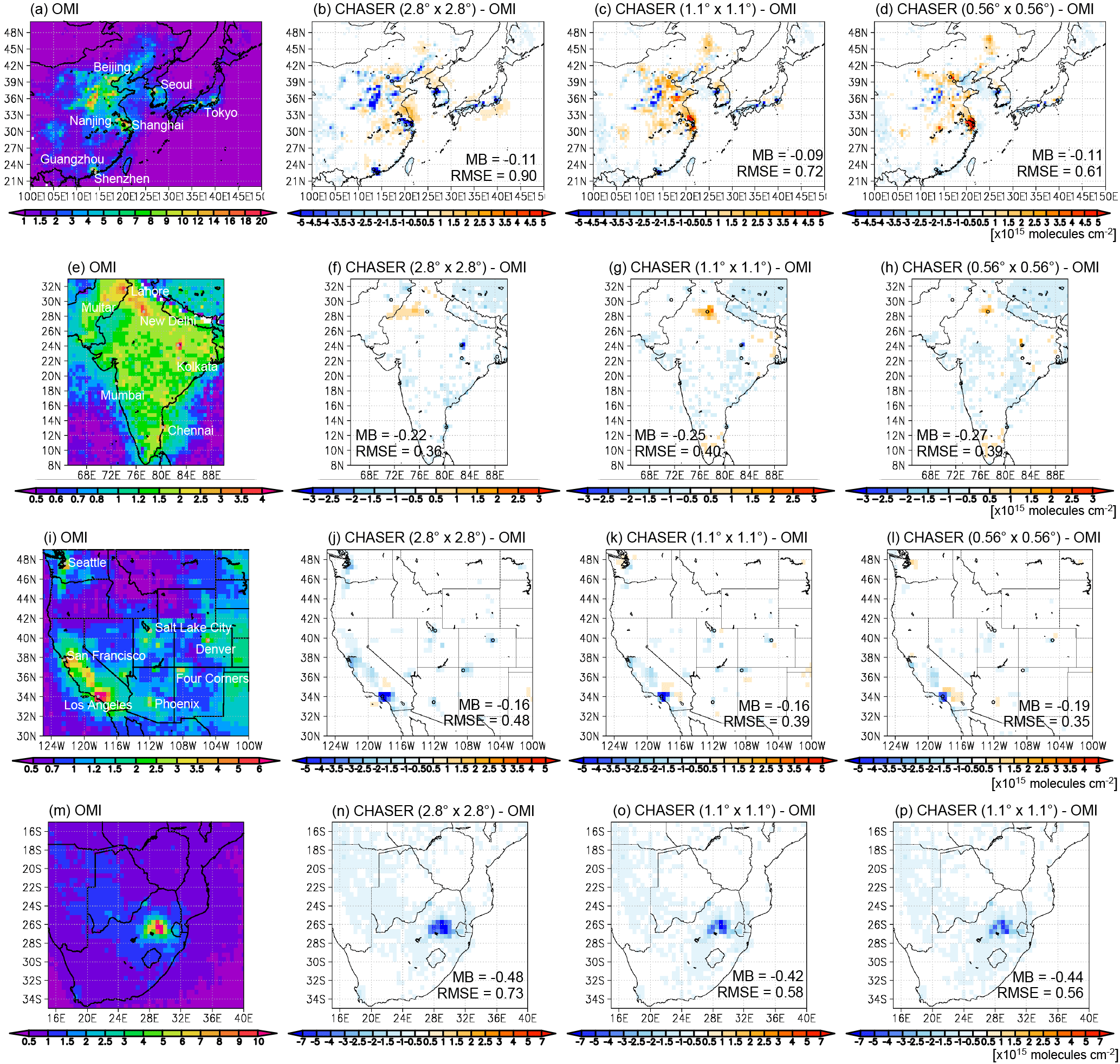
Figure 7Tropospheric NO2 column (× 1015 molecules cm−2) from OMI retrievals (first column; a, e, i, m) and differences between the model simulation at 2.8∘ (second column; b, f, j, n), 1.1∘ (third column; c, g, k, o), and 0.56∘ (fourth column; d, h, l, p) resolutions and OMI retrievals over East Asia (first row; a–d), South Asia (second row; e–h), and the western United States (third row; i–l) during JJA and over South Africa (forth row; m–p) during DJF 2008. Observed and simulated fields are mapped onto a 0.5∘ bin grid. Regional mean bias (MB) and RMSE are also shown.
Over South Asia, high concentrations were observed over large cities such as New Delhi, Chennai, Mumbai, and Kolkata in India, over Lahore and Multan in Pakistan, and around reported coal-based thermal power plants at 24∘ N, 83∘ E and 22∘ N, 83∘ E in India (Lu and Streets, 2012; Prasad et al., 2012). The 2.8∘ simulation was biased on the low side by up to 50 % over these areas, except westward of New Delhi, as commonly reported using another coarse-resolution model at 2.8∘ resolution (Sheel et al., 2010). These negative biases were reduced by up to 50 % at 1.1 and 0.56∘ resolutions, whereas high-resolution simulations reveal excessively high concentrations over New Delhi. Over rural areas, negative biases were larger at 1.1 and 0.56∘ resolutions, resulting in larger regional RMSE than at 2.8∘ resolution (see Sect. 4.1).
Over the western United States, high concentrations were observed around Los Angeles, San Francisco, Seattle, Phoenix, Salt Lake City, Denver, and the Four Corners and San Juan power plants. Negative biases were reduced with increasing model resolution over most of these regions. In contrast, negative biases remained at 0.56∘ resolution around strong local sources. Over rural areas, negative biases increased with model resolution, partly reflecting suppressed artificial dilution from strong local sources. As a result, regional RMSE was reduced by 18 and 27 % at 1.1 and 0.56∘ resolutions compared to 2.8∘ resolution. Errors, for instance, in soil NOx emissions in summer (e.g., Oikawa et al., 2015; Weber et al., 2015) could contribute to underestimations over rural areas.
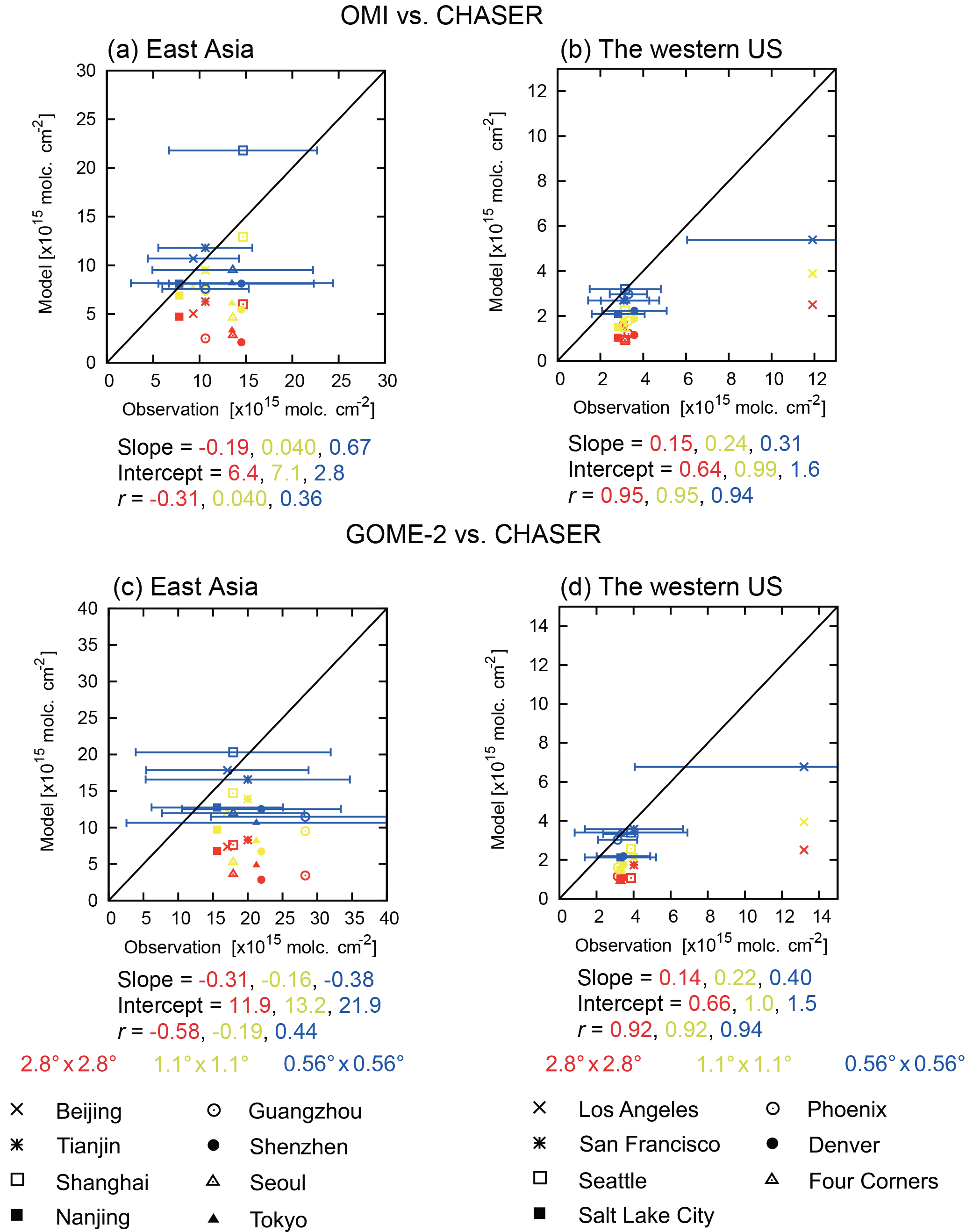
Figure 8Scatter plots of observed and simulated tropospheric NO2 column (× 1015 molecules cm−2) over strong local sources in East Asia (left column; a, c) and the western United States (right column; b, d) during JJA 2008 for the OMI retrievals (upper row; a–b) and GOME-2 retrievals (lower row; c–d). The red marks are the model simulation at 2.8∘ resolution, the yellow marks are the model simulation at 1.1∘ resolution, and the blue marks are the model simulation at 0.56∘ resolution. The horizontal bars indicate mean retrieval errors in OMI and GOME-2. For East Asia, the results are shown for Beijing (116.38∘ E, 39.92∘ N), Tianjin (117.18∘ E, 39.13∘ N), Shanghai (121.47∘ E, 31.23∘ N), Nanjing (118.77∘ E, 32.05∘ N), Guangzhou (113.27∘ E, 23.13∘ N), Shenzhen (114.10∘ E, 22.55∘ N), Seoul (126.96∘ E, 37.57∘ N), and Tokyo (139.68∘ E, 35.68∘ N). For the western United States, the results are shown for Los Angeles (118.25∘ W, 34.05∘ N), San Francisco (122.42∘ W, 37.78∘ N), Seattle (122.33∘ W, 47.61∘ N), Salt Lake City (111.88∘ E, 40.75∘ N), Phoenix (112.07∘ W, 33.45∘ N), Denver (104.88∘ W, 39.76∘ N), and the Four Corners and San Juan power plants (108.48∘ W, 36.69∘ N). The values and mean retrieval errors are averages within a 50 km distance from each strong source, with weighting function application based on the inverse of the distance from each location.
Over South Africa, high concentrations were observed over the Highveld region of South Africa, a complex source area, as noted in Sect. 4.1. The large negative bias (92 % at 2.8∘ resolution) in peak concentration over a power plant region in Mpumalanga Province (29.5∘ E, 26.2∘ S) was reduced to 69 % at 1.1∘ resolution and 53 % at 0.56∘ resolution. Negative bias (75 % at 2.8∘ resolution) in the Johannesburg–Pretoria megacity area (28∘ E, 25.7–26.2∘ S) was also reduced to 54 % at 1.1∘ resolution and 50 % at 0.56∘ resolution. High-resolution simulations are thus important for regions with complex and strong local sources. At the same time, the remaining negative bias at 0.56∘ suggests that power plant and industrial emissions are underestimated, as suggested by Miyazaki et al. (2017), or that a model resolution higher than 0.56∘ is essential.
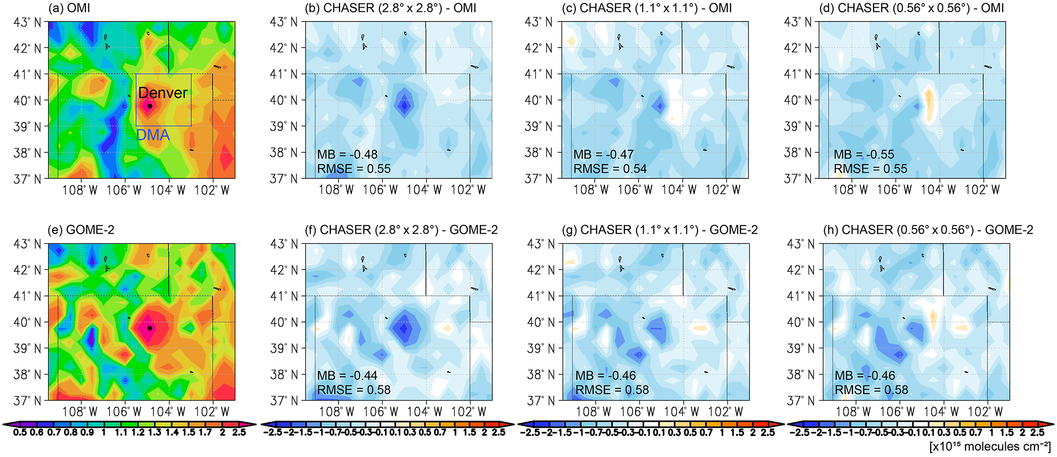
Figure 9Regional distributions of tropospheric NO2 column (× 1015 molecules cm−2) from satellite retrievals (first column; a, e) and differences between the model simulation at 2.8∘ (second column; b, f), 1.1∘ (third column; c, g), and 0.56∘ (fourth column; d, h) resolutions and satellite retrievals from OMI (upper row; a–d) and GOME-2 (lower row; e–h) over Colorado state during July–August 2014. The observed and simulated fields are mapped onto a 0.5∘ bin grid. The DMA area is shown by the blue square in (a).
Figure 8 compares simulated high NO2 concentrations with satellite retrievals at selected megacities. Eight strong source points were selected from East Asia and seven points from the western United States during June–July–August (JJA). We consider the summertime to be suitable for evaluating local NO2 pollution because of the short NO2 lifetime. For the comparisons, retrieved and simulated tropospheric NO2 columns were averaged within a 50 km distance from the selected points while applying a distance-based weighting function (i.e., the inverse of the distance was applied to each retrieval).
In comparison to OMI retrievals, with increasing model resolution, the slope for East Asia became closer to 1 (0.67 at 0.56∘ resolution and −0.19 at 2.8∘ resolution), and the intercept number became smaller (2.8 at 0.56∘ resolution and 6.4 at 2.8∘ resolution). The correlation coefficient also increased (r=0.36 at 0.56∘ resolution in contrast to at 2.8∘ resolution). Large negative biases were reduced at 0.56∘ resolution by 67 % over Beijing, by 73 % over Tianjin, by 18 % Shanghai, by 90 % over Nanjing, by 62 % over Guangzhou, by 48 % over Shenzhen, by 47 % over Seoul, and by 62 % over Tokyo (compared to 2.8∘ resolution). The estimated biases at 0.56∘ resolution are within mean OMI retrieval errors. Reductions in negative biases at 0.56∘ resolution against GOME-2 were also observed: by 91 % over Beijing, by 70 % over Tianjin, by 76 % over Shanghai, by 67 % over Nanjing, by 32 % over Guangzhou, by 50 % over Shenzhen, by 40 % over Seoul, and by 58 % over Tokyo. However, there is more degradation of slope and intercept against GOME-2 than against OMI, reflecting large negative biases over Guangzhou, Shenzhen, Seoul, and Tokyo.
Over the western United States, NO2 columns in all model simulations were in agreement with OMI retrievals (r>0.9). The 0.56∘ model reduced negative biases with respect to OMI by 30 % over Los Angeles, by 74 % over San Francisco, by 98 % over Seattle, by 58 % over Salt Lake City, by 83 % over Phoenix, by 44 % over Denver, and by 78 % over the Four Corners and San Juan power plants (compared to the 2.8∘ model). These bias reductions resulted in an improved slope number at 0.56∘ resolution (0.31) compared to 2.8∘ resolution (0.15). In this region, comparison results were generally similar between OMI and GOME-2. These validation results demonstrate the capability of the 0.56∘ simulation to represent high concentrations over strong local sources.
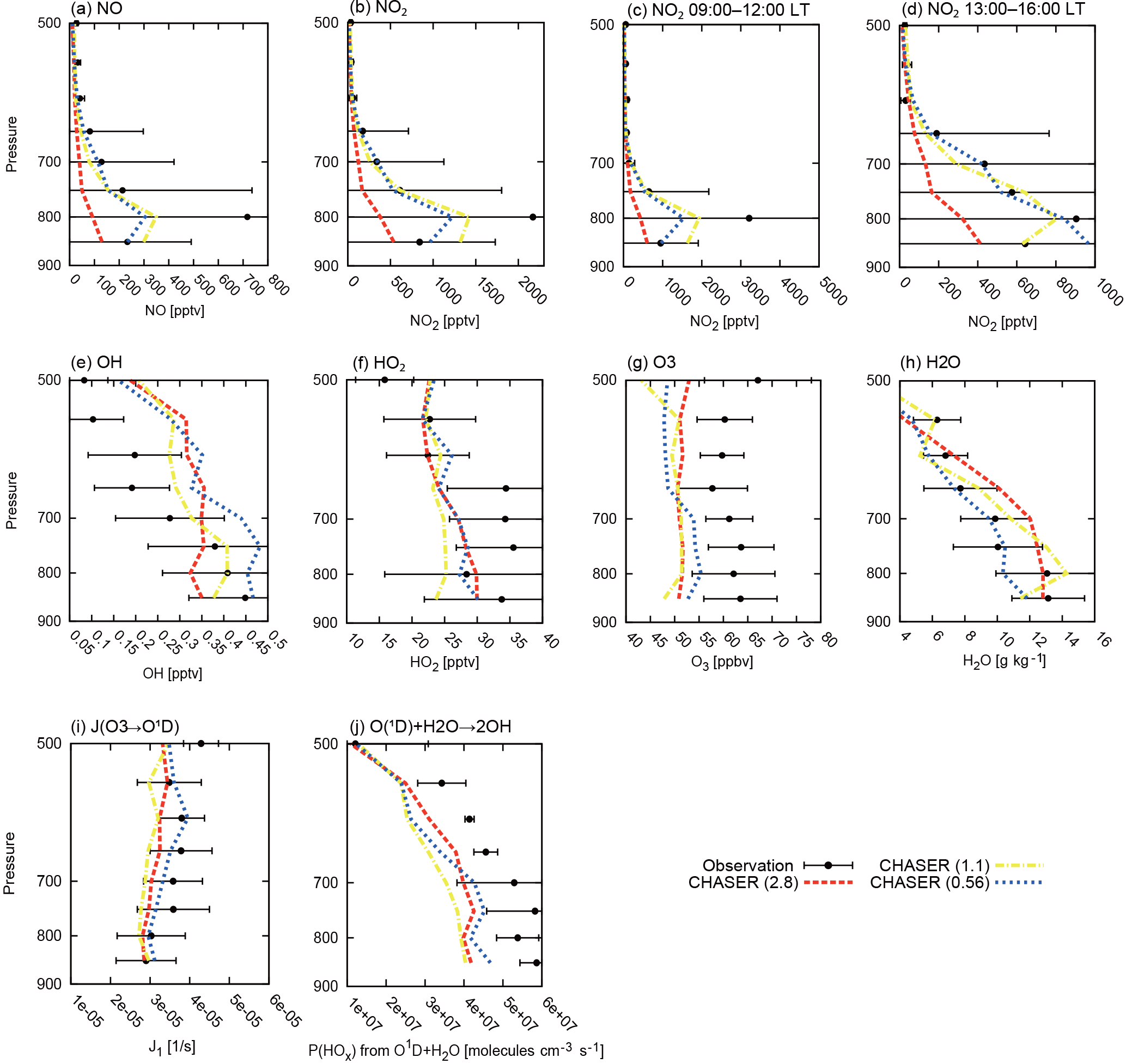
Figure 10Vertical profiles of NO (pptv) (a), NO2 (pptv) (b), NO2 during mornings (09:00–12:00 LT) (c) and afternoons (13:00–16:00 LT) (d), OH (pptv) (e), HO2 (pptv) (f), O3 (ppbv) (g), specific humidity (g kg−1) (h), the photolysis rate of O3 (s−1) (i), and the OH chemical production rate (molecules cm−3 s−1) from O1D and H2O (j) over the Denver metropolitan area (39–41∘ N and 103–105.5∘ W) during the FRAPPÉ period (from 16 July to 18 August 2014). The black dots represent the measurements, the red dashed line is the model simulation at 2.8∘ resolution, the yellow dashed-dotted line is the model simulation at 1.1∘ resolution, and the blue dotted line is the model simulation at 0.56∘ resolution. The horizontal bars represent the standard deviation of the measurements.
4.3 Validations using FRAPPÉ aircraft measurements
In this section, we evaluated model performance in relation to O3–HOx–NOx chemistry over the Denver metropolitan area (DMA; defined as 39–41∘ N and 103–105.5∘ W) in the western United States using the FRAPPÉ campaign observation data and satellite retrievals from July–August 2014. Figure 9 compares the spatial distribution of the tropospheric NO2 columns between simulations and satellite retrievals around the FRAPPÉ locations. OMI and GOME-2 observed high tropospheric NO2 columns over the DMA at around 40∘ N, 105∘ W. All models underestimated high concentrations by about 50 % at 2.8∘ resolution compared to OMI, with this declining by 37 % at 1.1∘ resolution and by 56 % at 0.56∘ resolution. The negative bias over the DMA was larger for GOME-2 than OMI, suggesting larger underestimations in simulated fields during mornings compared to afternoons. Outside the DMA, negative biases increased by 16 % for OMI and by 11 % for GOME-2 at 0.56∘ resolution compared to 2.8∘ resolution. As a result, RMSE against OMI and GOME-2 for the entire domain area was almost constant with varying model resolution.
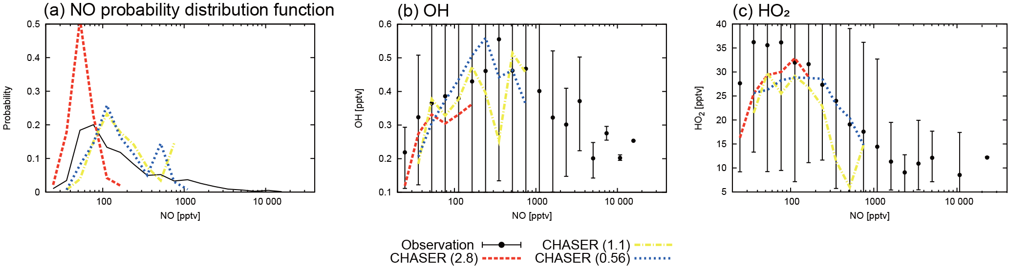
Figure 11(a) Probability distribution functions of NO, (b) OH, and (c) HO2 as a function of NO (pptv). The black dots represent measurements, the red dashed line is the model simulation at 2.8∘ resolution, the yellow dashed-dotted line is the model simulation at 1.1∘ resolution, and the blue dotted line is the model simulation at 0.56∘ resolution. The vertical bars represent the standard deviation of the measurements.
Figure 10 compares mean vertical profiles of trace gases and reaction rates over the DMA. Large negative biases of NO and NO2 at 2.8∘ resolution were mostly removed at 1.1 and 0.56∘ resolutions below 650 hPa (by up to 88 %), except at 800 hPa during daytime (09:00–16:00 LT). All simulations revealed large negative biases at 800 hPa during mornings (09:00–12:00 LT), but the bias was greater by 30 % at 2.8∘ resolution than at 1.1 and 0.56∘ resolutions. Afternoon lower tropospheric high concentrations (13:00–16:00 LT) were captured well in high-resolution simulations. Strong morning–afternoon variations in the lower troposphere were underestimated by 32 % at 0.56∘ resolution, by 48 % at 1.1∘ resolution, and by 62 % at 2.8∘ resolution. The remaining large bias in the morning at 0.56∘ resolution could be associated with insufficient vertical model resolution to represent mixing within nocturnal thin boundary layers.
Large negative OH biases at 2.8 and 1.1∘ resolutions at 850 hPa were reduced by 81 % at 0.56∘ resolution. From 800 to 750 hPa, the 1.1∘ simulation showed the closest agreement with observations (0.5–7 %), whereas the 2.8 and 0.56∘ simulations underestimated OH by 7–21 % and overestimated OH by up to 27 %, respectively. Above 700 hPa, all simulations overestimated OH with a factor of up to 2. All simulations also underestimated HO2 by 10–32 % below 650 hPa, except at 800 hPa.
OH and HO2 concentrations depend greatly on NOx concentrations through O3–HOx–NOx chemistry, as well as HOx production and OH conversion reactions to peroxy radicals (HO2 and RO2) with CO and VOCs. Figure 11a shows the probability distribution function of NO from the FRAPPÉ aircraft observation and the model simulations at 800 hPa over the DMA. The observation revealed a wide range of NO concentrations from 10–10 000 pptv. The 2.8∘ simulation overestimated the occurrence of concentrations < 100 pptv and underestimated the occurrence of concentrations > 100 pptv. The 1.1 and 0.56∘ simulations captured the observed probability distribution function, although they slightly overestimated the peak frequency concentration and underestimated the occurrence of low (< 100 pptv) and high (> 1000 pptv) concentrations. Figure 11b shows the OH–NO relationship used to validate O3–HOx–NOx chemistry. The observation showed OH increase with increasing NO to 350 pptv and a decrease with increasing NO from 350 pptv; all simulations captured the lower part (NO < 800 pptv) of the observed NO–OH relationship, suggesting that the model realistically simulates nonlinear O3–HOx–NOx chemistry. The lack of high NO (> 800 pptv) with low OH resulted in an overestimation of mean OH concentrations at 0.56∘ resolution.
Figure 11c compares the HO2–NO relationship. All simulations underestimated the occurrence of high HO2 (> 25 pptv) at low NO (< 100 pptv). This implies an underestimation of HOx chemical production in the simulations. We evaluated HOx production from the chemical reaction of O(1D) with H2O using temperature, specific humidity, O3 photolysis rate to O(1D) (J), and O3 concentration with the assumption of O(1D) equilibrium (Fig. 10g–j). All simulations underestimated HOx production, with the underestimation being smaller by 13 % at 0.56∘ resolution at 800 hPa. The underestimation of HOx production was primarily attributable to a negative bias in O3 by 11 % and J by 2.5 % at 0.56∘ resolution at 800 hPa. The negative biases of O3 and J were reduced by 39 and 58 %, respectively, at 0.56∘ (compared to 2.8∘) resolution. Biases in specific humidity also had small impacts on calculated HOx production. Positive biases of specific humidity at 2.8∘ resolution above 750 hPa were reduced by up to 83 % at 0.56∘ resolution. The lack of nitrous acid (HONO) in the model could explain a component of the HOx production underestimation, especially during mornings (e.g., Kanaya et al., 2001). The underestimation of OH conversion to peroxy radicals could also explain simulated errors in OH and HO2. Griffith et al. (2016) attributed OH overprediction and HO2 underprediction in a box model simulation to underestimation of total OH reactivity (i.e., missing OH sink) over the United States.
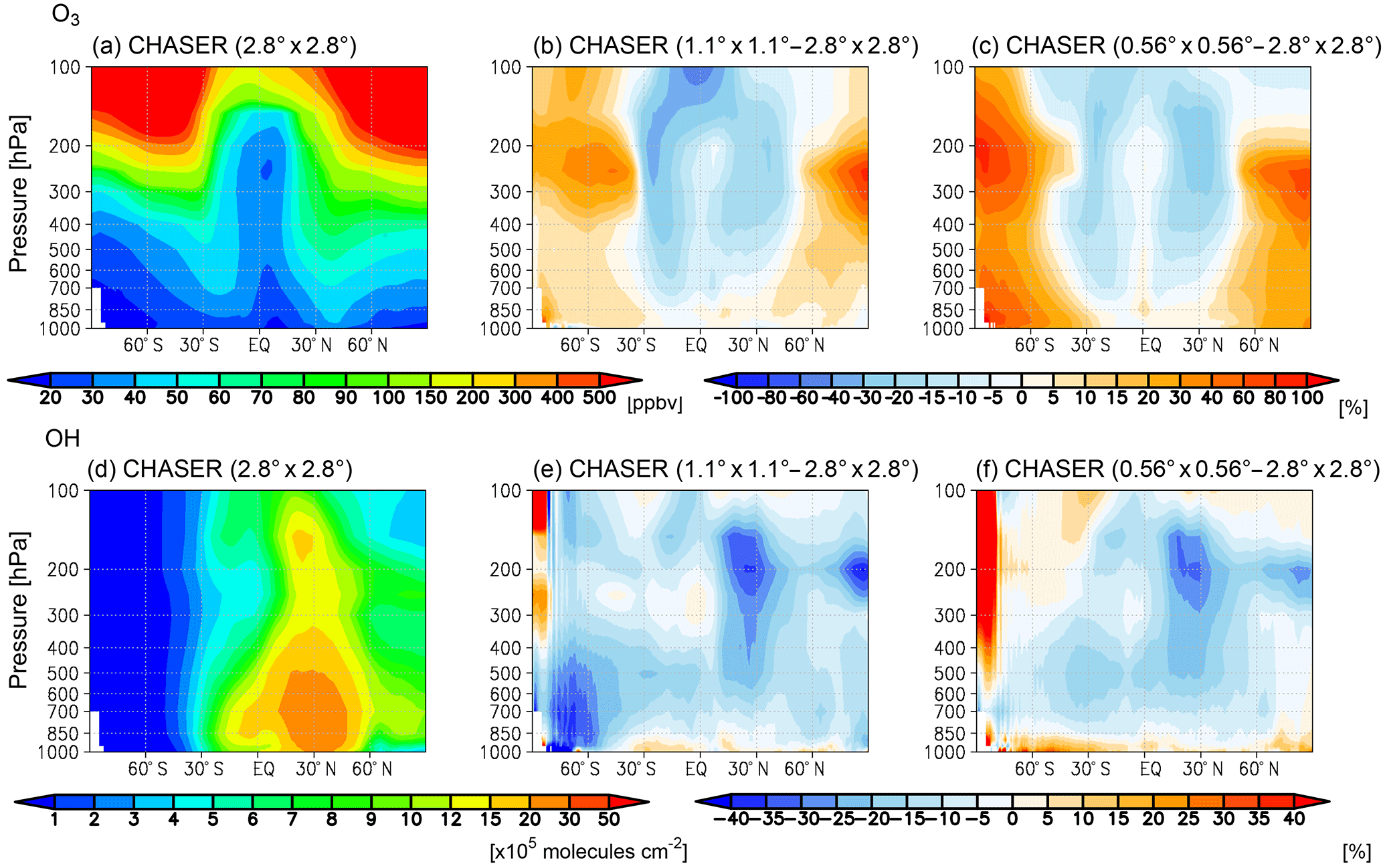
Figure 12Latitude–pressure distribution of zonal mean (a–c) O3 (ppbv) and (d–f) OH (× 105 molecules cm−3) in the model simulation at 2.8∘ (left column) during JJA in 2008 and differences between the model simulation at 1.1∘ (middle column) and 0.56∘ (right column) resolutions and the model at 2.8∘ resolution.
The 2014 simulations used the anthropogenic emission inventory for the year 2010 (see Sect. 2.1). The optimized NOx emissions from an assimilation of multiple species satellite measurements (Miyazaki et al., 2017) suggest that surface NOx emissions over the DMA in July–August increased by 7 % from 2010 to 2014. The temporal variation, together with large uncertainties in the emission inventories, could explain part of the negative biases of NO and NO2 at 800 hPa, which also affects OH, HO2, and O3 through nonlinear chemistry processes.
We analyzed the simulated global distribution of O3, OH, and NOx in the year 2008 to characterize the resolution dependence of NO2-related chemistry. Figure 12 compares zonal mean concentrations of O3 and OH during JJA. O3 mixing ratios in the middle to high latitudes were 10–60 % larger at 1.1 and 0.56∘ than at 2.8∘ resolution. As shown in Table 2, at 1.1 and 0.56∘ resolutions, negative biases against ozonesonde observations were reduced by up to 8 ppbv at 850 hPa from middle to high latitudes in both hemispheres and by up to 13 ppbv at 500 hPa in the Southern Hemisphere (SH) and Northern Hemisphere (NH) middle and high latitudes. In contrast, positive model biases in the upper troposphere and lower stratosphere (UTLS) mostly increased with model resolution by up to 46 ppbv at 300 hPa in the SH and NH high latitudes. The increased positive bias at high latitudes in the UTLS was associated with strengthened downwelling, as will be discussed below. RMSE against ozonesonde was reduced by up to 8 ppbv at 850 and 500 hPa in middle and high latitudes, except at 500 hPa in the NH high latitudes.
Table 2Comparisons of seasonal mean tropospheric O3 concentration during JJA in 2008 between ozonesonde and the model simulation at 2.8, 1.1, and 0.56∘ resolutions. Units are ppbv.
In the tropics and subtropics, in contrast, O3 concentrations were 5–20 % lower at 1.1 and 0.56∘ than at 2.8∘ resolution, reducing positive biases against ozonesonde observations from 2.8∘ resolution by 15 ppbv at 850 hPa in the tropics (30∘ S–30∘ N) and by up to 15 ppbv at 300 hPa in the midlatitudes of both hemispheres. In contrast, negative biases increased by 7 ppbv at 500 hPa and by 9 ppbv at 300 hPa in the tropics. RMSE was smaller by 10 ppbv at 0.56∘ than at 2.8∘ resolution at 300 hPa in the SH midlatitudes. Substantial improvements were achieved from the tropopause to lower stratosphere (i.e., at 100 hPa) by using high-resolution simulations. Overall, RMSE with respect to the globally available ozonesondes was reduced with increasing resolution (by up to 8.1 ppbv) at 850 and 500 hPa. In contrast, at 300 hPa, RMSE increased at 0.56∘ (by 1.2 ppbv) and 1.1∘ (by 9.4 ppbv) resolutions, reflecting larger RMSE at 0.56 and 1.1∘ resolutions in the high latitudes of both hemispheres.
Increased concentrations in the extratropics and decreased concentrations in the tropics resulted in only small differences in the global tropospheric ozone burden: −5.4 % at 1.1∘ resolution and −2.3 % at 0.56∘ resolution (compared to 2.8∘). Meanwhile, the budget terms of global tropospheric O3 differ significantly between simulations. High-resolution models simulated an enhanced stratosphere–troposphere exchange (STE) of O3 (510 Tg yr−1 at 1.1∘ resolution and 548 Tg yr−1 at 0.56∘ resolution in contrast to 500 Tg yr−1 at 2.8∘ resolution) and smaller O3 chemical production (4647 Tg yr−1 at 1.1∘ resolution and 4565 Tg yr−1 at 0.56∘ resolution in contrast to 4809 Tg yr−1 at 2.8∘ resolution). Less O3 chemical production was attributed to decelerating HO2 + NO, CH3O2 + NO, and RO2 + NO. The estimated global mean O3 chemical lifetime was longer in high-resolution simulations (26.1 days at 1.1∘ resolution and 26.3 days at 0.56∘ resolution in contrast to 25.3 days at 2.8∘ resolution) because of decreased water vapor in the middle and upper troposphere. Model resolution dependence on global STE and ozone chemical production has been similarly reported by Wild and Prather (2006), Stock et al. (2014), Yan et al. (2016), and Williams et al. (2017). The latitudinal distributions of O3 differences between simulations were determined by both chemical (e.g., weakened chemical ozone production in the tropics) and transport (e.g., strengthened downwelling from extratropical stratosphere and upper tropospheric poleward motions from the tropics to the extratropics) processes.
OH was smaller by 5–30 % at 1.1 and 0.56∘ than at 2.8∘ resolution in the tropics and subtropics during JJA, resulting in smaller global burdens of tropospheric OH by 13.5 % at 1.1∘ resolution and by 12.4 % at 0.56∘ resolution. These changes were associated with decreased HOx chemical production (i.e., O(1D) + H2O → 2OH) and HO2 to OH conversion reaction (i.e., HO2 + NO → OH + NO2) by 5 % at 1.1 and 0.56∘ resolutions (compared to 2.8∘ resolution). A large relative OH increment was found over the Antarctic because weak ultraviolet radiation led to small OH concentrations during a polar night.
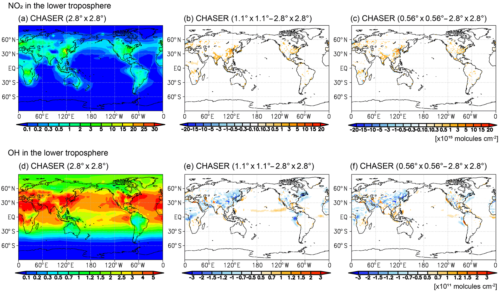
Figure 13Global distributions of (a–c) NO2 partial column (× 1015 molecules cm−2) and (d–f) OH partial column (× 1011 molecules cm−2) integrated in the lowermost five model layers in the model simulation at 2.8∘ resolution (first column) during JJA in 2008 and differences between the model simulation at 1.1∘ (second column) and 0.56∘ (third column) resolutions and the model at 2.8∘ resolution.
Table 3Regional net chemical production of NOx via all reactions and HNO3 formation (Tg yr−1), NO2 burden (Gg), NO2 lifetime via HNO3 formation reaction (hours) in the lowermost five model layers, and planetary boundary layer (PBL) height (m) in the model simulations and ERA-Interim. The definition of the regions is the same as in Fig. 3.
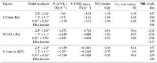
Figure 13 compares the spatial distribution of NO2 and OH in the lower troposphere between model simulations. Lower tropospheric NO2 partial columns were larger around strong source areas and smaller over rural and coastal areas around polluted regions at 1.1 and 0.56∘ resolutions, primarily resulting from suppressed artificial dilution near strong sources and chemical feedback through the O3–HOx–NOx system, as discussed in Sect. 4. The lower tropospheric OH partial column integrated in the lowermost five model layers (approximately below 800 hPa) was smaller at 1.1 and 0.56∘ resolutions over most of the continents. The differences in OH and NO2 exhibited similar spatial patterns over polluted and biomass burning regions: e.g., r=0.53 over the western United States, r=0.61 over India, and r=0.57 over South America. NO2 and OH thus interact with each other through O3–HOx–NOx chemical reactions. Differences in simulated meteorological fields, such as cumulus convection, water vapor, and cloud cover, could also cause OH differences.
Table 3 summarizes the chemical budget of NO2 in the lowermost five model layers over eastern China, the western United States, and South America during summertime in each hemisphere. Over the selected regions, the NO2 burden increased with model resolution by 33 % over eastern China, by 9 % over the western United States, and by 23 % over South America. Over eastern China and the western United States, the conversion from NO2 to HNO3 with OH (P–L(NOx)) dominated over the net chemical production of NOx (P–L(NOx)). The estimated NO2 lifetime via HNO3 formation (1 ∕ k[OH][M]) was 8 % longer at 0.56∘ than at 2.8∘ resolution. A longer NO2 lifetime with increasing model resolution over East Asia is consistently reported by Wild and Prather (2006). Over the western United States, the estimated NO2 lifetime was longer by 6 % at 1.1∘ than at 2.8∘ resolution, whereas it was shorter by 6 % at 0.56∘ than at 1.1∘ resolution. Over South America, the conversion of NO2 to HNO3 contributed 13–20 % of the total net chemical production of NOx, resulting from competition against chemical conversion to peroxy acetyl nitrates (PANs) and organic nitrates. The estimated NO2 lifetime via HNO3 formation was longer by 18 % at 0.56∘ than at 2.8∘ resolution. Over other regions, the regional NO2 burden increased with model resolution, whereas changes in NO2 lifetime via OH oxidation varied across locations (not shown), reflecting a nonlinear chemical system involving NOx (Valin et al., 2011).
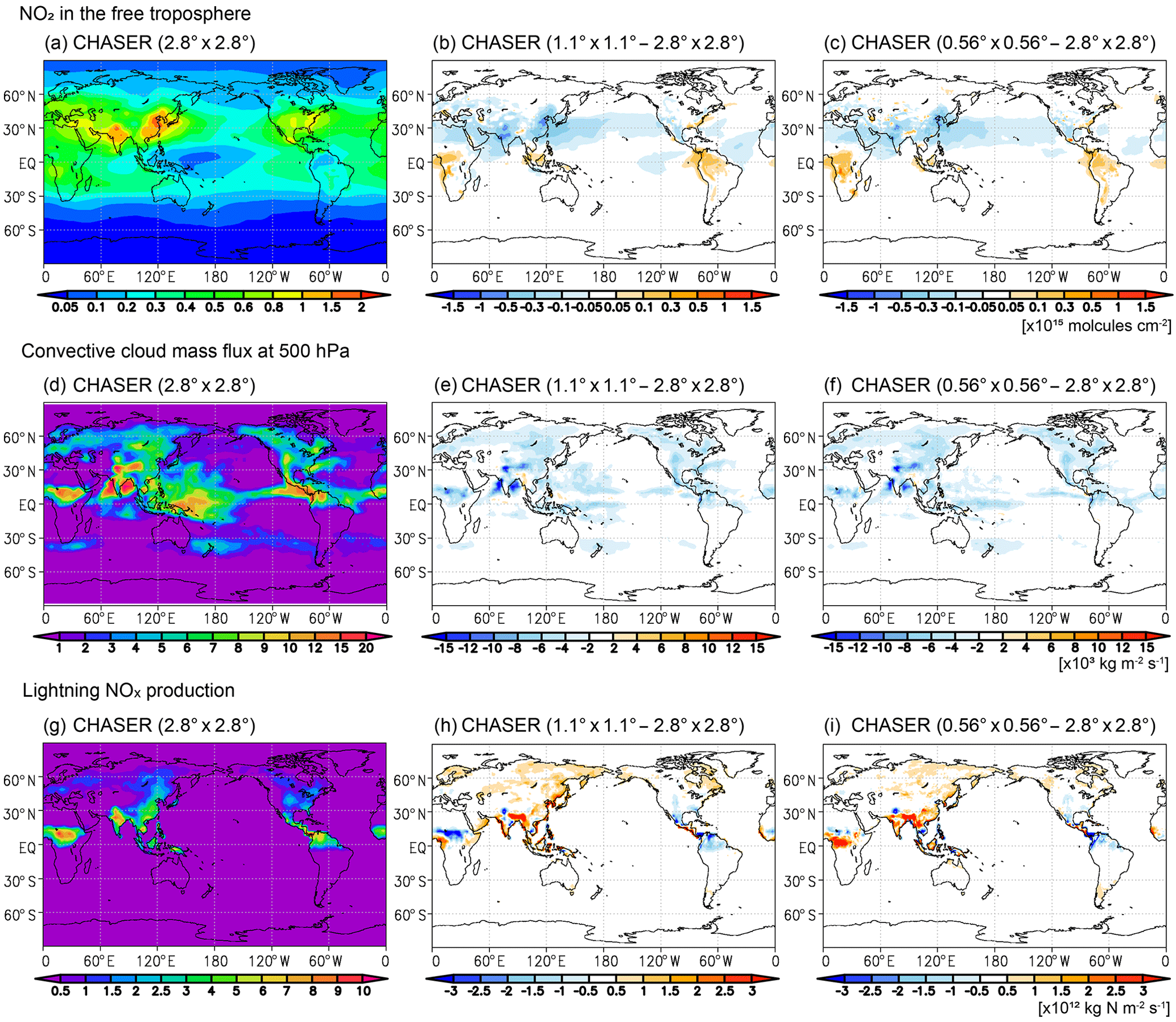
Figure 14Global distributions of (a–c) NO2 partial column (× 1015 molecules cm−2) integrated from the sixth layer to the tropopause, (d–f) convective cloud updraft (× 103 kg m−2 s−1) at 500 hPa, and (g–i) vertically integrated lightning NOx production (× 1012 kg N m−2 s−1) in the model simulation at 2.8∘ resolution (first column) during JJA in 2008 and differences between the model simulation at 1.1∘ (second column) and 0.56∘ (third column) resolutions and the model at 2.8∘ resolution.
Differences in simulated meteorological fields between simulations could also have effects on NO2 and related species. Improvements in PBL height are especially expected to improve NO2 simulations in the lower troposphere (e.g., Lin and McElroy, 2010). Table 3 compares regional mean PBL height over eastern China, the western United States, and South America in summer between ERA-Interim reanalysis and the model simulations. The 2.8∘ simulation overestimated regional mean PBL height in ERA-Interim; the positive bias was reduced at 0.56∘ resolution by 40 % over eastern China, by 62 % over the western United States, and by 9 % over South America.
Figure 14 shows the spatial distribution of the NO2 partial column in the free troposphere, convective cloud updraft mass flux at 500 hPa, and vertically integrated lightning NOx production. The simulated NO2 partial column in the free troposphere was smaller by 17 % at 1.1∘ resolution and by 14 % at 0.56∘ resolution than at 2.8∘ resolution over the northern subtropics and midlatitudes, primarily because of smaller NO2 concentrations above 400 hPa. These changes in the free tropospheric NO2 were in contrast to the changes in the lower tropospheric NO2, which were associated with suppressed convective cloud updraft over the continents by up to 76 % at 1.1 and 0.56∘ resolutions over the northern subtropics and midlatitudes. In contrast, over the Maritime Continent, South America, and Central Africa, the free tropospheric NO2 column was larger at 1.1∘ resolution by up to 18 % and at 0.56∘ resolution by up to 20 % than at 2.8∘ resolution, primarily reflecting increased NO2 concentration between 600 and 800 hPa. Lightning NOx production is also largely different between the simulations in the tropics. Over the tropics, although the mean convective cloud updraft was weaker at 1.1 and 0.56∘ resolutions than at 2.8∘ resolution, the high-resolution simulations revealed increased ice cloud in the upper troposphere and stronger (but less frequent) convection, thus increasing lightning NOx sources, especially over Asia. Meanwhile, given the same amount of lightning NOx production (using a commonly prescribed lightning NOx field in all the simulations), the high-resolution simulations revealed slightly less ozone chemical production (by 1 %) through the representation of local highly concentrated NOx plumes in July 2008 (figure not shown).
The obtained evaluation results of multiple species and meteorological fields suggest that changes in NO2 with increasing model resolution can be due to complex chemical interactions and different representations of meteorological fields. Further detailed validations of individual components would therefore be helpful to identify causal mechanisms and to further reduce uncertainty in high-resolution simulations.
6.1 Other model error sources
Various factors other than horizontal model resolution can lead to errors in tropospheric NO2 simulation. Insufficient vertical model resolution could introduce additional errors in vertical mixing, atmospheric transport, and subsequent chemistry processes, for instance, under stable boundary layer conditions during nighttime (Menut et al., 2013). Such errors could also cause large negative NO2 biases during mornings in the lower troposphere (see Sect. 4.3). More detailed validation of diurnal variations is required using ground-based observations such as MAX-DOAS and lidar in future work.
Chemical kinetics information could also have large uncertainties. Lin et al. (2012) and Stavrakou et al. (2013) suggested that the uptake of HO2 on aerosols is the most important factor but remains largely uncertain. CHASER includes simplified NOx–VOC chemistry related to PANs and isoprene nitrates (Sudo et al., 2002). The incorporation of more detailed NOx–VOC chemistry would also be needed to improve simulated peroxy nitrates and organic nitrates, as per Ito et al. (2007, 2009) and Fischer et al. (2014).
Surface emissions are another important error source. The total amounts of anthropogenic NOx emissions in China in 2008 differ by 27 % between two (highest and lowest) bottom-up inventories: EDGAR4.2 and MEIC (Saikawa et al., 2017). Ding et al. (2017a) also discussed large diversity in emission inventories over East Asia. Biomass burning NOx emissions also differ significantly between inventories: for example, the annual mean emission is 2.293 Tg yr−1 in GFASv1.0 in contrast to 2.700 Tg yr−1 in GFEDv3.1 over the SH Africa, as reported by Kaiser et al. (2012).
Based on data assimilation of multiple species satellite measurements, Miyazaki et al. (2017) investigated large uncertainty in anthropogenic and fire-related emission factors and a significant underestimation of soil NOx sources in bottom-up emission inventories. Using a similar approach, Miyazaki et al. (2014) optimized lightning NOx sources and indicated that the widely used lightning parameterization based on the C-shape assumption (Price and Rind, 1992; Pickering et al., 1998) has large uncertainty. Implementing these optimized emissions could improve model performance, although optimal emissions could also be dependent on model resolution.
Representations of meteorological parameters, such as cloud optical depth, temperature, water vapor, PBL height, and relevant transport and chemical processes, are also important in tropospheric NO2 simulations (Lin et al., 2012). Because we employed an AGCM–CTM online coupling system, meteorological fields are simulated explicitly at each model resolution. This could help to improve the tropospheric chemistry simulation. For instance, we found that simulated regional mean PBL height is sensitive to the choice of model resolution, with the 0.56∘ simulation showing closer agreements with ERA-Interim reanalysis, as discussed in Sect. 4.3. Resolving small-scale cloud distributions may lead to improved photolysis and convective transport calculations in high-resolution simulations.
Nevertheless, the AGCM meteorological fields still need to be carefully validated and improved. For instance, cumulus convection and cloud parameterization calculations were sensitive to model resolution. Although the relevant model parameters have been optimized separately for each model resolution, there are still some discrepancies against observed OLR and precipitation distributions (see Sect. 2).
6.2 Nonlinearity in model error reductions
Model performance was clearly better at 0.56 and 1.1∘ resolutions than at 2.8∘ resolution in most cases. The 0.56∘ simulation largely improved spatial variations over eastern China, the eastern and western United States, Mexico, and South Africa, as confirmed by large RMSE reductions, especially for megacities and regions with power plants (see Sect. 4). In most cases, the improvement was smaller from 1.1 to 0.56∘ resolution than from 2.8 to 1.1∘ resolution. Meanwhile, regional RMSEs increased at 0.56∘ from 1.1∘ resolution for some cases over Europe, India, and the selected biomass burning regions, possibly related to more pronounced errors in meteorological fields for Europe and India and in biomass burning hot spot emissions.
Comparisons to aircraft measurements showed better performance of NOx simulation at high resolutions. However, the representation of NO variability (i.e., the probability distribution function) was insufficient even at 0.56∘ resolution. Further improvements could be obtained using a model with resolution finer than 0.56∘. For instance, Valin et al. (2011) noted that 4 and 12 km resolutions are required for Four Corners and Los Angeles, respectively, to accurately simulate the nonlinear chemical feedback of the O3–HOx–NOx system. Yamaji et al. (2014) reported that errors in the simulated tropospheric NO2 column at 20 km resolution did not yet approach convergence over Tokyo.
Most previous high-resolution modeling studies have used regional models to simulate NO2 concentration fields at high spatial resolution, primarily focusing on urban regions, with reduced or equivalent computational costs compared to global models. Several studies have demonstrated that a better representation of the long-range transport of NOx reservoir species such as peroxyacetyl nitrate (PAN) are important on simulated NO2 in the free troposphere in remote areas (e.g., Hudman et al., 2004; Fischer et al., 2010, 2014; Jiang et al., 2016). A two-way nesting between regional and coarse-resolution global models (e.g., Yan et al., 2016) is able to consider both small-scale processes inside focusing regions and long-range transport over the globe, which has an advantage over regional models. An important advantage of global high-resolution models over regional models and two-way nesting systems is the ability to simulate NO2 concentration fields at high resolutions over the entire globe across urban, biomass burning, and remote regions in a consistent framework. Even over remote regions, a high-resolution simulation has the potential to improve model performance through considering the effects of nonlinear chemistry in highly concentrated NOx plumes emitted from ships and lightning (Charlton-Perez et al., 2009; Vinken et al., 2011; Gressent et al., 2016). These NOx emission sources in remote regions have significant impacts on climate and air quality (Eyring et al., 2010; Holmes et al., 2014; Banerjee et al., 2014; Finney et al., 2016). It is thus important to clarify the importance of resolving small-scale sources and plumes within a global modeling framework for a better understanding of the global atmospheric environment and chemistry–climate system.
Williams et al. (2017) also showed that the differences in NO2 profiles between the TM5-MP model at 3∘ × 2∘ and 1∘ × 1∘ horizontal resolutions are within a few percentage points below 850 hPa over the Pacific in boreal spring. They also showed much larger differences with changing model resolution over Texas in autumn. Model resolution impact thus varies significantly with location and season. Further investigations using other aircraft measurements would be helpful to evaluate model performance in different cases.
High-resolution chemical transport modeling requires huge computational resources: e.g., compared to the simulation at 2.8∘ resolution (approximately 480 s computer time for a 1-day simulation), the computational cost increased by a factor of 67 at 0.56∘ resolution (approximately 32 000 s computer time) and by a factor of 14 at 1.1∘ resolution (approximately 6700 s computer time). High-performance computing (HPC) systems are thus essential for performing high-resolution simulations. At the same time, because the size of a 3-D array is large in the high-resolution model, computational efficiency is important: e.g., efficient data throughputs in memory transfer, network communication between multiple nodes, and file input–output. In the future, further improvements in computational efficiency will be required, together with the development of HPC systems.
6.3 Application for satellite retrieval and data assimilation
An important application of high-resolution tropospheric NO2 simulations is to provide a priori profile information on satellite retrieval and chemical data assimilation (Liu et al., 2017). Here, we would like to discuss the potentials of the obtained results for these applications.
Current satellite retrievals of the tropospheric NO2 column use a priori NO2 profiles obtained from global model simulations at relatively coarse resolutions: from TM5 at 3∘ × 2∘ in DOMINO-2 (Boersma et al., 2011) and GEOS-Chem at 2.5∘ × 2∘ in OMNO2 (Bucsela et al., 2006; Celarier et al., 2008), whereas the TROPOMI retrieval product will employ 1∘ × 1∘ resolution simulation fields from TM5 (Williams et al., 2017). To provide high-resolution (ranging from 4 to 50 km) a priori information, several regional retrievals have employed regional models (Heckel et al., 2011; Russell et al., 2011; Lin et al., 2014), showing improvements in the retrieved fields in comparison to independent observations. High-resolution a priori fields from global CTMs are important in providing consistent global datasets.
To avoid spatial representation gaps between satellite measurements and coarse-resolution global models, super-observation techniques have been employed to produce representative data before assimilation (e.g., Miyazaki et al., 2012). The average of averaging kernels over a number of retrievals within a super-observation grid does not hold any physical meaning. This may inhibit effective improvement by assimilating over regions with varying conditions. High-resolution CTMs allow for the assimilation of satellite measurements, with reduced representation gaps without any averages.
Because of the distinct nonlinearity in chemical reactions, the high-resolution assimilation of satellite measurements considering small-scale variations in background error covariance would be essential in making the best use of observational information. High-resolution chemical data assimilation could also benefit air pollutant emission estimates (e.g., Miyazaki et al., 2014, 2017; Liu et al., 2017), especially using high-resolution measurements from future satellite missions such as TOROPOMI and geostationary satellites (e.g., Sentinel-4, GEMS, TEMPO), even when model resolution is still coarser than the measurement resolution through improved model processes and spatial representativeness for mega-cities as demonstrated by this study.
We evaluated the performance of high-resolution global NO2 simulations using CHASER based on comparisons against tropospheric NO2 column retrievals from two satellite sensors, OMI and GOME-2, and aircraft observations during the FRAPPÉ aircraft campaign. Three different horizontal resolutions at 0.56, 1.1, and 2.8∘ were evaluated.
The high-resolution models at 1.1 and 0.56∘ resolutions showed substantial improvements in simulating tropospheric NO2. With increasing horizontal model resolution from 2.8 to 1.1∘, negative regional mean model biases (RMSEs) for annual mean tropospheric NO2 column were reduced over polluted regions: e.g., by 90 % (32 %) over eastern China, by 13 % (20 %) over the western United States, and by 37 % (45 %) over South Africa. RMSEs were further reduced by increasing model resolution from 1.1 to 0.56∘ over most of the polluted regions. We emphasize large error reductions from 1.1 to 0.56∘ resolutions by 23 % over the western United States, by 25 % over Mexico, and by 20 % over South Africa. The high-resolution simulation at 0.56∘ was also essential to capture observed high tropospheric NO2 columns over strong sources such as megacities and power plants. In comparison to OMI, increasing model resolution from 2.8 to 0.56∘ reduced negative biases over strong local sources by 67 % over Beijing, by 47 % over Seoul, by 62 % over Tokyo, by 30 % over Los Angeles, by 74 % over San Francisco, and by 78 % over the Four Corners and San Juan power plants in summer. Over biomass burning regions, model performance also improved with increasing model resolution from 2.8 to 1.1∘ and 0.56∘. For instance, RMSE was reduced by 15 % at 1.1∘ resolution (compared to 2.8∘ resolution) over South America. We attempted to distinguish between two different effects that led to improvements in high-resolution modeling: (1) closer spatial representativeness between observations and simulations (up to approximately 0.5∘ resolution) and (2) better representation of large-scale (i.e., at 2.8∘) concentration fields through the consideration of small-scale processes, for instance, associated with nonlinear O3–HOx–NOx chemistry. The relative contributions of these two effects were mostly identical over the eastern and western United States and South Africa, whereas the latter effect (2) was dominant over eastern China and biomass burning regions.
The comparison to FRAPPÉ aircraft observations over the DMA indicated that the 0.56∘ simulation greatly reduced negative biases of NO2 by up to 88 % from the surface to 650 hPa, while improving the representation of morning–afternoon differences below 800 hPa (with a 50 % reduction at 1.1∘ resolution). The high-resolution simulations also improved the probability distribution of NO concentration ranging from 100–1000 pptv. However, all simulations failed to reproduce the observed low (< 100 pptv) and high (> 1000 pptv) NO concentrations, resulting in positive biases of mean OH through nonlinear NO–OH relationships.
Changes in NO2 across model simulations were associated with different representations of the tropospheric chemical and transport system. By increasing model resolution from 2.8 to 0.56∘, tropospheric ozone increased by up to 60 % in middle to high latitudes during JJA, while ozone decreased by up to 20 % in the tropics and subtropics. These changes mostly led to improved agreements against the global ozonesonde measurements. The high-resolution simulation also lowered OH concentrations throughout the troposphere by up to 30 %. The regional NO2 burden was larger at 0.56∘ than at 2.8∘ in the lower troposphere, by 33 % over eastern China, by 9 % over the western United States, and by 23 % over South America. Changes in NO2 lifetime via oxidation with OH varied between locations. These model resolution dependencies suggest that NO2 and OH interact with each other through nonlinear relationships between NO and OH (i.e., O3–HOx–NOx chemistry).
In conclusion, the 1.1∘ simulation generally captures the regional distribution of the tropospheric NO2 column well, but the 0.56∘ resolution is essential for the simulation of high NO2 concentrations on a megacity scale. Meanwhile, for Europe, India, and the selected biomass burning regions, errors increased with model resolution from 1.1 to 0.56∘, possibly related to more pronounced errors in meteorological fields over Europe and India and to more pronounced influences of largely uncertain inventories for individual burning points over the selected biomass burning regions. The computational cost largely increases at 0.56∘ resolution, while overall improvements were small at 0.56∘ resolution compared to 1.1∘ resolution except over megacities. Therefore, we consider the horizontal resolution of approximately 1∘ to be a realistic option to obtain improved overall performance of global tropospheric NO2 simulations.
The developed high-resolution CTM framework will be a powerful tool when combined with future high-resolution satellite observations, providing valuable information on the atmospheric environment and related long-term changes on the megacity scale. We are developing a high-resolution global chemical data assimilation system based on an ensemble Kalman filter data assimilation technique (Miyazaki et al., 2017) and the developed high-resolution CTM. A post-petascale supercomputer, also known as a post-K computer, is being developed by Japan's FLAGSHIP 2020 project (e.g., Miyoshi et al., 2015) and will facilitate future studies using the high-resolution global chemical data assimilation system and satellite observations from a new constellation of low Earth orbit sounders (e.g., IASI, AIRS, CrIS, TROPOMI, and Sentinel-5) and geostationary satellites (e.g., Sentinel-4, GEMS, and TEMPO).
The source code for CHASER V4.0 is not publicly available because of license restrictions. The source code can be obtained from Kengo Sudo (kengo@nagoya-u.jp) upon request. Most of the source code is written in Fortran 77 and 90. The simulation data will be available upon request to the corresponding author. Satellite retrievals of the tropospheric NO2 column from OMI and GOME-2 were obtained from the TEMIS website (http://www.temis.nl/). Measurement data from the 2014 FRAPPÉ campaign were provided at the NASA LaRC Air-borne Science Data for Atmospheric Composition (http://www-air.larc.nasa.gov/). GPCP combined precipitation data were downloaded from the NASA GSFC global precipitation analysis website (https://precip.gsfc.nasa.gov/). Ozonesonde data were obtained from WOUDC (https://woudc.org/), SHADOZ (https://tropo.gsfc.nasa.gov/shadoz/), and NOAA ESRL GMD (https://www.esrl.noaa.gov/gmd/). Interpolated OLR from NOAA 18 was provided at NOAA ESRL PSD (https://www.esrl.noaa.gov/psd/).
The authors declare that they have no conflict of interest.
This work was supported by the post-K computer project Priority Issue 4 (the
advancement of meteorological and global environmental predictions utilizing
observational Big Data) and by the Global Environment Research Fund (S-12) of
the Ministry of the Environment (MOE). We acknowledge the use of tropospheric
NO2 column data from GOME-2 and OMI sensors obtained from the
Tropospheric Emission Monitoring Internet Service
(http://www.temis.nl/index.php). We would also like to express our
thanks for the use of measurement data from the 2014 Front Range Air
Pollution and Photochemistry Experiment (FRAPPÉ) campaign through the NASA
LaRC Airborne Science Data for Atmospheric Composition
(https://www-air.larc.nasa.gov/). The GPCP combined precipitation data
were provided by the NASA Goddard Space Flight Center's Laboratory for
Atmospheres, which developed the data as a contribution to the GEWEX Global
Precipitation Climatology Project. We would like to acknowledge the use of
ozonesonde data obtained from the World Ozone and Ultraviolet Data Center
(WOUDC), the Southern Hemisphere ADditional Ozonesondes (SHADOZ), and the
NOAA Earth System Research Laboratory (ESRL) Global Monitoring Division
(GMD). Interpolated OLR data were provided by the NOAA/OAR/ESRL PSD from
their website (http://www.esrl.noaa.gov/psd/). The Earth
Simulator was used for simulations
as a “Strategic Project with Special Support” of the Japan Agency for
Marine-Earth Science and Technology. Some simulations were also conducted by
the K computer provided by the RIKEN Advanced Institute for Computational
Science through the HPCI System Research Project (project IDs: hp150288,
hp160231, hp170232). We would like to thank the two anonymous reviewers for
their useful comments.
Edited by: Andrea
Stenke
Reviewed by: two anonymous referees
Adler, R. F., Huffman, G. J., Chang, A., Ferraro, R., Xie, P.-P., Janowiak, J., Rudolf, B., Schneider, U., Curtis, S., Bolvin, D., Gruber, A., Susskind, J., Arkin, P., and Nelkin, E.: The Version-2 Global Precipitation Climatology Project (GPCP) Monthly Precipitation Analysis (1979–Present), J. Hydrometeorol., 4, 1147–1167, https://doi.org/10.1175/1525-7541(2003)004<1147:TVGPCP>2.0.CO;2, 2003. a
Akiyoshi, H., Zhou, L. B., Yamashita, Y., Sakamoto, K., Yoshiki, M., Nagashima, T., Takahashi, M., Kurokawa, J., Takigawa, M., and Imamura, T.: A CCM simulation of the breakup of the Antarctic polar vortex in the years 1980–2004 under the CCMVal scenarios, J. Geophys. Res., 114, D03103, https://doi.org/10.1029/2007JD009261, 2009. a
Akiyoshi, H., Nakamura, T., Miyasaka, T., Shiotani, M., and Suzuki, M.: A nudged chemistry-climate model simulation of chemical constituent distribution at northern high-latitude stratosphere observed by SMILES and MLS during the 2009/2010 stratospheric sudden warming, J. Geophys. Res., 121, 1361–1380, https://doi.org/10.1002/2015JD023334, 2015JD023334, 2016. a
Arellano Jr., A. F., Raeder, K., Anderson, J. L., Hess, P. G., Emmons, L. K., Edwards, D. P., Pfister, G. G., Campos, T. L., and Sachse, G. W.: Evaluating model performance of an ensemble-based chemical data assimilation system during INTEX-B field mission, Atmos. Chem. Phys., 7, 5695–5710, https://doi.org/10.5194/acp-7-5695-2007, 2007. a
Banerjee, A., Archibald, A. T., Maycock, A. C., Telford, P., Abraham, N. L., Yang, X., Braesicke, P., and Pyle, J. A.: Lightning NOx, a key chemistry–climate interaction: impacts of future climate change and consequences for tropospheric oxidising capacity, Atmos. Chem. Phys., 14, 9871–9881, https://doi.org/10.5194/acp-14-9871-2014, 2014. a
Boersma, K. F., Eskes, H. J., and Brinksma, E. J.: Error analysis for tropospheric NO2 retrieval from space, J. Geophys. Res., 109, D04311, https://doi.org/10.1029/2003JD003962, 2004. a
Boersma, K. F., Jacob, D. J., Eskes, H. J., Pinder, R. W., Wang, J., and van der A, R. J.: Intercomparison of SCIAMACHY and OMI tropospheric NO2 columns: Observing the diurnal evolution of chemistry and emissions from space, J. Geophys. Res., 113, D16S26, https://doi.org/10.1029/2007JD008816, 2008. a
Boersma, K. F., Eskes, H. J., Dirksen, R. J., van der A, R. J., Veefkind, J. P., Stammes, P., Huijnen, V., Kleipool, Q. L., Sneep, M., Claas, J., Leitão, J., Richter, A., Zhou, Y., and Brunner, D.: An improved tropospheric NO2 column retrieval algorithm for the Ozone Monitoring Instrument, Atmos. Meas. Tech., 4, 1905–1928, https://doi.org/10.5194/amt-4-1905-2011, 2011. a, b, c, d
Brown, S. S., Ryerson, T. B., Wollny, A. G., Brock, C. A., Peltier, R., Sullivan, A. P., Weber, R. J., Dubé, W. P., Trainer, M., Meagher, J. F., Fehsenfeld, F. C., and Ravishankara, A. R.: Variability in Nocturnal Nitrogen Oxide Processing and Its Role in Regional Air Quality, Science, 311, 67–70, https://doi.org/10.1126/science.1120120, 2006. a, b
Bucsela, E. J., Celarier, E. A., Wenig, M. O., Gleason, J. F., Veefkind, J. P., Boersma, K. F., and Brinksma, E. J.: Algorithm for NO2 vertical column retrieval from the ozone monitoring instrument, IEEE Trans. Geosci. Remote Sens., 44, 1245–1258, https://doi.org/10.1109/TGRS.2005.863715, 2006. a
Canty, T. P., Hembeck, L., Vinciguerra, T. P., Anderson, D. C., Goldberg, D. L., Carpenter, S. F., Allen, D. J., Loughner, C. P., Salawitch, R. J., and Dickerson, R. R.: Ozone and NOx chemistry in the eastern US: evaluation of CMAQ/CB05 with satellite (OMI) data, Atmos. Chem. Phys., 15, 10965–10982, https://doi.org/10.5194/acp-15-10965-2015, 2015. a
Castellanos, P., Boersma, K. F., Torres, O., and de Haan, J. F.: OMI tropospheric NO2 air mass factors over South America: effects of biomass burning aerosols, Atmos. Meas. Tech., 8, 3831–3849, https://doi.org/10.5194/amt-8-3831-2015, 2015. a
Celarier, E. A., Brinksma, E. J., Gleason, J. F., Veefkind, J. P., Cede, A., Herman, J. R., Ionov, D., Goutail, F., Pommereau, J.-P., Lambert, J.-C., van Roozendael, M., Pinardi, G., Wittrock, F., Schönhardt, A., Richter, A., Ibrahim, O. W., Wagner, T., Bojkov, B., Mount, G., Spinei, E., Chen, C. M., Pongetti, T. J., Sander, S. P., Bucsela, E. J., Wenig, M. O., Swart, D. P. J., Volten, H., Kroon, M., and Levelt, P. F.: Validation of Ozone Monitoring Instrument nitrogen dioxide columns, J. Geophys. Res., 113, D15S15, https://doi.org/10.1029/2007JD008908, 2008. a
Charlton-Perez, C. L., Evans, M. J., Marsham, J. H., and Esler, J. G.: The impact of resolution on ship plume simulations with NOx chemistry, Atmos. Chem. Phys., 9, 7505–7518, https://doi.org/10.5194/acp-9-7505-2009, 2009. a
Colella, P. and Woodward, P. R.: The Piecewise Parabolic Method (PPM) for gas-dynamical simulations, J. Comput. Phys., 54, 174–201, https://doi.org/10.1016/0021-9991(84)90143-8, 1984. a
Dee, D. P., Uppala, S. M., Simmons, A. J., Berrisford, P., Poli, P., Kobayashi, S., Andrae, U., Balmaseda, M. A., Balsamo, G., Bauer, P., Bechtold, P., Beljaars, A. C. M., van de Berg, I., Biblot, J., Bormann, N., Delsol, C., Dragani, R., Fuentes, M., Greer, A. J., Haimberger, L., Healy, S. B., Hersbach, H., Holm, E. V., Isaksen, L., Kallberg, P., Kohler, M., Matricardi, M., McNally, A. P., Mong-Sanz, B. M., Morcette, J.-J., Park, B.-K., Peubey, C., de Rosnay, P., Tavolato, C., Thepaut, J. N., and Vitart, F.: The ERA-Interim reanalysis: Configuration and performance of the data assimilation system, Q. J. Roy. Meteorol. Soc., 137, 553–597, https://doi.org/10.1002/qj.828, 2011. a
Dentener, F. J. and Crutzen, P. J.: Reaction of N2O5 on tropospheric aerosols: Impact on the global distributions of NOx, O3, and OH, J. Geophys. Res., 98, 7149–7163, https://doi.org/10.1029/92JD02979, 1993. a
Ding, J., Miyazaki, K., van der A, R. J., Mijling, B., Kurokawa, J.-I., Cho, S., Janssens-Maenhout, G., Zhang, Q., Liu, F., and Levelt, P. F.: Intercomparison of NOx emission inventories over East Asia, Atmos. Chem. Phys., 17, 10125–10141, https://doi.org/10.5194/acp-17-10125-2017, 2017a. a
Ding, J., van der A, R. J., Mijling, B., and Levelt, P. F.: Space-based NOx emission estimates over remote regions improved in DECSO, Atmos. Meas. Tech., 10, 925–938, https://doi.org/10.5194/amt-10-925-2017, 2017b. a
Duce, R. A., LaRoche, J., Altieri, K., Arrigo, K. R., Baker, A. R., Capone, D. G., Cornell, S., Dentener, F., Galloway, J., Ganeshram, R. S., Geider, R. J., Jickells, T., Kuypers, M. M., Langlois, R., Liss, P. S., Liu, S. M., Middelburg, J. J., Moore, C. M., Nickovic, S., Oschlies, A., Pedersen, T., Prospero, J., Schlitzer, R., Seitzinger, S., Sorensen, L. L., Uematsu, M., Ulloa, O., Voss, M., Ward, B., and Zamora, L.: Impacts of Atmospheric Anthropogenic Nitrogen on the Open Ocean, Science, 320, 893–897, https://doi.org/10.1126/science.1150369, 2008. a
Duncan, B. N., Lamsal, L. N., Thompson, A. M., Yoshida, Y., Lu, Z., Streets, D. G., Hurwitz, M. M., and Pickering, K. E.: A space-based, high-resolution view of notable changes in urban NOx pollution around the world (2005–2014), J. Geophys. Res., 121, 976–996, https://doi.org/10.1002/2015JD024121, 2016. a, b
Emori, S., Nozawa, T., Numaguti, A., and Uno, I.: Importance of Cumulus Parameterization for Precipitation Simulation over East Asia in June, J. Meteorol. Soc. Jpn., 79, 939–947, https://doi.org/10.2151/jmsj.79.939, 2001. a
Evans, M. J. and Jacob, D. J.: Impact of new laboratory studies of N2O5 hydrolysis on global model budgets of tropospheric nitrogen oxides, ozone, and OH, Geophys. Res. Lett., 32, L09813, https://doi.org/10.1029/2005GL022469, 2005. a
Eyring, V., Isaksen, I. S., Berntsen, T., Collins, W. J., Corbett, J. J., Endresen, O., Grainger, R. G., Moldanova, J., Schlager, H., and Stevenson, D. S.: Transport impacts on atmosphere and climate: Shipping, Atmos. Environ., 44, 4735–4771, https://doi.org/10.1016/j.atmosenv.2009.04.059, 2010. a
Finney, D. L., Doherty, R. M., Wild, O., Young, P. J., and Butler, A.: Response of lightning NOx emissions and ozone production to climate change: Insights from the Atmospheric Chemistry and Climate Model Intercomparison Project, Geophys. Res. Lett., 43, 5492–5500, https://doi.org/10.1002/2016GL068825, 2016. a
Fischer, E. V., Jaffe, D. A., Reidmiller, D. R., and Jaeglé, L.: Meteorological controls on observed peroxyacetyl nitrate at Mount Bachelor during the spring of 2008, J. Geophys. Res., 115, D03302, https://doi.org/10.1029/2009JD012776, 2010. a
Fischer, E. V., Jacob, D. J., Yantosca, R. M., Sulprizio, M. P., Millet, D. B., Mao, J., Paulot, F., Singh, H. B., Roiger, A., Ries, L., Talbot, R. W., Dzepina, K., and Pandey Deolal, S.: Atmospheric peroxyacetyl nitrate (PAN): a global budget and source attribution, Atmos. Chem. Phys., 14, 2679–2698, https://doi.org/10.5194/acp-14-2679-2014, 2014. a, b
Giglio, L., Randerson, J. T., and van der Werf, G. R.: Analysis of daily, monthly, and annual burned area using the fourth-generation global fire emissions database (GFED4), J. Geophys. Res., 118, 317–328, https://doi.org/10.1002/jgrg.20042, 2013. a
Gressent, A., Sauvage, B., Cariolle, D., Evans, M., Leriche, M., Mari, C., and Thouret, V.: Modeling lightning-NOx chemistry on a sub-grid scale in a global chemical transport model, Atmos. Chem. Phys., 16, 5867–5889, https://doi.org/10.5194/acp-16-5867-2016, 2016. a
Griffith, S. M., Hansen, R. F., Dusanter, S., Michoud, V., Gilman, J. B., Kuster, W. C., Veres, P. R., Graus, M., de Gouw, J. A., Roberts, J., Young, C., Washenfelder, R., Brown, S. S., Thalman, R., Waxman, E., Volkamer, R., Tsai, C., Stutz, J., Flynn, J. H., Grossberg, N., Lefer, B., Alvarez, S. L., Rappenglueck, B., Mielke, L. H., Osthoff, H. D., and Stevens, P. S.: Measurements of hydroxyl and hydroperoxy radicals during CalNex-LA: Model comparisons and radical budgets, J. Geophys. Res., 121, 4211–4232, https://doi.org/10.1002/2015JD024358, 2016. a
Gruber, N. and Galloway, J. N.: An Earth-system perspective of the global nitrogen cycle, Nature, 451, 293–296, https://doi.org/10.1038/nature06592, 2008. a
Guenther, A., Karl, T., Harley, P., Wiedinmyer, C., Palmer, P. I., and Geron, C.: Estimates of global terrestrial isoprene emissions using MEGAN (Model of Emissions of Gases and Aerosols from Nature), Atmos. Chem. Phys., 6, 3181–3210, https://doi.org/10.5194/acp-6-3181-2006, 2006. a
Han, K. M., Lee, S., Chang, L. S., and Song, C. H.: A comparison study between CMAQ-simulated and OMI-retrieved NO2 columns over East Asia for evaluation of NOx emission fluxes of INTEX-B, CAPSS, and REAS inventories, Atmos. Chem. Phys., 15, 1913–1938, https://doi.org/10.5194/acp-15-1913-2015, 2015. a
Harkey, M., Holloway, T., Oberman, J., and Scotty, E.: An evaluation of CMAQ NO2 using observed chemistry-meteorology correlations, J. Geophys. Res., 120, 11775–11797, https://doi.org/10.1002/2015JD023316, 2015JD023316, 2015. a
Heckel, A., Kim, S.-W., Frost, G. J., Richter, A., Trainer, M., and Burrows, J. P.: Influence of low spatial resolution a priori data on tropospheric NO2 satellite retrievals, Atmos. Meas. Tech., 4, 1805–1820, https://doi.org/10.5194/amt-4-1805-2011, 2011. a, b
Hess, P. G. and Vukicevic, T.: Intercontinental transport, chemical transformations, and baroclinic systems, J. Geophys. Res., 108, 4354, https://doi.org/10.1029/2002JD002798, 2003. a
Holmes, C. D., Prather, M. J., and Vinken, G. C. M.: The climate impact of ship NOx emissions: an improved estimate accounting for plume chemistry, Atmos. Chem. Phys., 14, 6801–6812, https://doi.org/10.5194/acp-14-6801-2014, 2014. a
Hudman, R. C., Jacob, D. J., Cooper, O. R., Evans, M. J., Heald, C. L., Park, R. J., Fehsenfeld, F., Flocke, F., Holloway, J., Hübler, G., Kita, K., Koike, M., Kondo, Y., Neuman, A., Nowak, J., Oltmans, S., Parrish, D., Roberts, J. M., and Ryerson, T.: Ozone production in transpacific Asian pollution plumes and implications for ozone air quality in California, J. Geophys. Res., 109, D23S10, https://doi.org/10.1029/2004JD004974, 2004. a
Huffman, G. J., Adler, R. F., Bolvin, D. T., and Gu, G.: Improving the global precipitation record: GPCP Version 2.1, Geophys. Res. Lett., 36, https://doi.org/10.1029/2009GL040000, 2009. a
Huijnen, V., Eskes, H. J., Poupkou, A., Elbern, H., Boersma, K. F., Foret, G., Sofiev, M., Valdebenito, A., Flemming, J., Stein, O., Gross, A., Robertson, L., D'Isidoro, M., Kioutsioukis, I., Friese, E., Amstrup, B., Bergstrom, R., Strunk, A., Vira, J., Zyryanov, D., Maurizi, A., Melas, D., Peuch, V.-H., and Zerefos, C.: Comparison of OMI NO2 tropospheric columns with an ensemble of global and European regional air quality models, Atmos. Chem. Phys., 10, 3273–3296, https://doi.org/10.5194/acp-10-3273-2010, 2010a. a, b, c
Huijnen, V., Williams, J., van Weele, M., van Noije, T., Krol, M., Dentener, F., Segers, A., Houweling, S., Peters, W., de Laat, J., Boersma, F., Bergamaschi, P., van Velthoven, P., Le Sager, P., Eskes, H., Alkemade, F., Scheele, R., Nédélec, P., and Pätz, H.-W.: The global chemistry transport model TM5: description and evaluation of the tropospheric chemistry version 3.0, Geosci. Model Dev., 3, 445–473, https://doi.org/10.5194/gmd-3-445-2010, 2010b. a, b
Inness, A., Blechschmidt, A.-M., Bouarar, I., Chabrillat, S., Crepulja, M., Engelen, R. J., Eskes, H., Flemming, J., Gaudel, A., Hendrick, F., Huijnen, V., Jones, L., Kapsomenakis, J., Katragkou, E., Keppens, A., Langerock, B., de Mazière, M., Melas, D., Parrington, M., Peuch, V. H., Razinger, M., Richter, A., Schultz, M. G., Suttie, M., Thouret, V., Vrekoussis, M., Wagner, A., and Zerefos, C.: Data assimilation of satellite-retrieved ozone, carbon monoxide and nitrogen dioxide with ECMWF's Composition-IFS, Atmos. Chem. Phys., 15, 5275–5303, https://doi.org/10.5194/acp-15-5275-2015, 2015. a
IPCC: Climate Change 2013: The Physical Science Basis, Contribution of Working Group I to the Fifth Assessment Report of the Intergovernmental Panel on Climate Change, Cambridge University Press, Cambridge, UK, New York, NY, USA, https://doi.org/10.1017/CBO9781107415324, 2013. a
Irie, H., Boersma, K. F., Kanaya, Y., Takashima, H., Pan, X., and Wang, Z. F.: Quantitative bias estimates for tropospheric NO2 columns retrieved from SCIAMACHY, OMI, and GOME-2 using a common standard for East Asia, Atmos. Meas. Tech., 5, 2403–2411, https://doi.org/10.5194/amt-5-2403-2012, 2012. a
Itahashi, S., Uno, I., Irie, H., Kurokawa, J.-I., and Ohara, T.: Regional modeling of tropospheric NO2 vertical column density over East Asia during the period 2000–2010: comparison with multisatellite observations, Atmos. Chem. Phys., 14, 3623–3635, https://doi.org/10.5194/acp-14-3623-2014, 2014. a
Ito, A., Sillman, S., and Penner, J. E.: Effects of additional nonmethane volatile organic compounds, organic nitrates, and direct emissions of oxygenated organic species on global tropospheric chemistry, J. Geophys. Res., 112, D06309, https://doi.org/10.1029/2005JD006556, 2007. a
Ito, A., Sillman, S., and Penner, J. E.: Global chemical transport model study of ozone response to changes in chemical kinetics and biogenic volatile organic compounds emissions due to increasing temperatures: Sensitivities to isoprene nitrate chemistry and grid resolution, J. Geophys. Res., 114, D09301, https://doi.org/10.1029/2008JD011254, 2009. a
Janssens-Maenhout, G., Crippa, M., Guizzardi, D., Dentener, F., Muntean, M., Pouliot, G., Keating, T., Zhang, Q., Kurokawa, J., Wankmüller, R., Denier van der Gon, H., Kuenen, J. J. P., Klimont, Z., Frost, G., Darras, S., Koffi, B., and Li, M.: HTAP_v2.2: a mosaic of regional and global emission grid maps for 2008 and 2010 to study hemispheric transport of air pollution, Atmos. Chem. Phys., 15, 11411–11432, https://doi.org/10.5194/acp-15-11411-2015, 2015. a, b
Jiang, Z., Worden, J. R., Payne, V. H., Zhu, L., Fischer, E., Walker, T., and Jones, D. B. A.: Ozone export from East Asia: The role of PAN, J. Geophys. Res., 121, 6555–6563, https://doi.org/10.1002/2016JD024952, 2016. a
K-1 model developers: K-1 Coupled GCM (MIROC) Description, Tech. rep., Center for Climate System Research (Univ. of Tokyo), National Institute for Environmental Studies, and Frontier Research Center for Global Change, available at: http://ccsr.aori.u-tokyo.ac.jp/~hasumi/miroc_description.pdf, 2004. a, b
Kaiser, J. W., Heil, A., Andreae, M. O., Benedetti, A., Chubarova, N., Jones, L., Morcrette, J.-J., Razinger, M., Schultz, M. G., Suttie, M., and van der Werf, G. R.: Biomass burning emissions estimated with a global fire assimilation system based on observed fire radiative power, Biogeosciences, 9, 527–554, https://doi.org/10.5194/bg-9-527-2012, 2012. a
Kanaya, Y., Matsumoto, J., Kato, S., and Akimoto, H.: Behavior of OH and HO2 radicals during the Observations at a Remote Island of Okinawa (ORION99) field campaign: 2. Comparison between observations and calculations, J. Geophys. Res., 106, 24209–24223, https://doi.org/10.1029/2000JD000179, 2001. a
Kim, S.-W., Heckel, A., Frost, G. J., Richter, A., Gleason, J., Burrows, J. P., McKeen, S., Hsie, E.-Y., Granier, C., and Trainer, M.: NO2 columns in the western United States observed from space and simulated by a regional chemistry model and their implications for NOx emissions, J. Geophys. Res., 114, D11301, https://doi.org/10.1029/2008JD011343, 2009. a, b
Krotkov, N. A., McLinden, C. A., Li, C., Lamsal, L. N., Celarier, E. A., Marchenko, S. V., Swartz, W. H., Bucsela, E. J., Joiner, J., Duncan, B. N., Boersma, K. F., Veefkind, J. P., Levelt, P. F., Fioletov, V. E., Dickerson, R. R., He, H., Lu, Z., and Streets, D. G.: Aura OMI observations of regional SO2 and NO2 pollution changes from 2005 to 2015, Atmos. Chem. Phys., 16, 4605–4629, https://doi.org/10.5194/acp-16-4605-2016, 2016. a
Levelt, P. F., van den Oord, G. H. J., Dobber, M. R., Malkki, A., Visser, H., de Vries, J., Stammes, P., Lundell, J. O. V., and Saari, H.: The ozone monitoring instrument, IEEE Trans. Geosci. Remote Sens., 44, 1093–1101, https://doi.org/10.1109/TGRS.2006.872333, 2006. a
Li, D. and Shine, K.: A 4-dimensional ozone climatology for UGAMP models, UGAMP Internal Rep., 35, 35, 1995. a
Liebmann, B.: Description of a complete (interpolated) outgoing longwave radiation dataset, B. Am. Meteorol. Soc., 77, 1275–1277, 1996. a
Lin, J.-T. and McElroy, M. B.: Impacts of boundary layer mixing on pollutant vertical profiles in the lower troposphere: Implications to satellite remote sensing, Atmos. Environ., 44, 1726–1739, https://doi.org/10.1016/j.atmosenv.2010.02.009, 2010. a
Lin, J.-T., Liu, Z., Zhang, Q., Liu, H., Mao, J., and Zhuang, G.: Modeling uncertainties for tropospheric nitrogen dioxide columns affecting satellite-based inverse modeling of nitrogen oxides emissions, Atmos. Chem. Phys., 12, 12255–12275, https://doi.org/10.5194/acp-12-12255-2012, 2012. a, b
Lin, J.-T., Martin, R. V., Boersma, K. F., Sneep, M., Stammes, P., Spurr, R., Wang, P., Van Roozendael, M., Clémer, K., and Irie, H.: Retrieving tropospheric nitrogen dioxide from the Ozone Monitoring Instrument: effects of aerosols, surface reflectance anisotropy, and vertical profile of nitrogen dioxide, Atmos. Chem. Phys., 14, 1441–1461, https://doi.org/10.5194/acp-14-1441-2014, 2014. a, b
Lin, S.-J. and Rood, R. B.: Multidimensional Flux-Form Semi-Lagrangian Transport Schemes, Mon. Weather Rev., 124, 2046–2070, https://doi.org/10.1175/1520-0493(1996)124<2046:MFFSLT>2.0.CO;2, 1996. a
Liu, F., Zhang, Q., Tong, D., Zheng, B., Li, M., Huo, H., and He, K. B.: High-resolution inventory of technologies, activities, and emissions of coal-fired power plants in China from 1990 to 2010, Atmos. Chem. Phys., 15, 13299–13317, https://doi.org/10.5194/acp-15-13299-2015, 2015. a
Liu, X., Mizzi, A. P., Anderson, J. L., Fung, I. Y., and Cohen, R. C.: Assimilation of satellite NO2 observations at high spatial resolution using OSSEs, Atmos. Chem. Phys., 17, 7067–7081, https://doi.org/10.5194/acp-17-7067-2017, 2017. a, b, c
Lu, Z. and Streets, D. G.: Increase in NOx Emissions from Indian Thermal Power Plants during 1996–2010: Unit-Based Inventories and Multisatellite Observations, Environ. Sci. Technol., 46, 7463–7470, https://doi.org/10.1021/es300831w, 2012. a
Mauldin, R. L., Cantrell, C. A., Zondlo, M., Kosciuch, E., Eisele, F. L., Chen, G., Davis, D., Weber, R., Crawford, J., Blake, D., Bandy, A., and Thornton, D.: Highlights of OH, H2SO4, and methane sulfonic acid measurements made aboard the NASA P-3B during Transport and Chemical Evolution over the Pacific, J. Geophys. Res., 108, 8796, https://doi.org/10.1029/2003JD003410, 2003. a
Mellor, G. L. and Yamada, T.: A Hierarchy of Turbulence Closure Models for Planetary Boundary Layers, J. Atmos. Sci., 31, 1791–1806, https://doi.org/10.1175/1520-0469(1974)031<1791:AHOTCM>2.0.CO;2, 1974. a
Menut, L., Bessagnet, B., Colette, A., and Khvorostiyanov, D.: On the impact of the vertical resolution on chemistry-transport modelling, Atmos. Environ., 67, 370–384, https://doi.org/10.1016/j.atmosenv.2012.11.026, 2013. a, b
Mijling, B. and van der A, R. J.: Using daily satellite observations to estimate emissions of short-lived air pollutants on a mesoscopic scale, J. Geophys. Res., 117, D17302, https://doi.org/10.1029/2012JD017817, 2012. a
Miyazaki, K., Eskes, H. J., and Sudo, K.: Global NOx emission estimates derived from an assimilation of OMI tropospheric NO2 columns, Atmos. Chem. Phys., 12, 2263–2288, https://doi.org/10.5194/acp-12-2263-2012, 2012. a, b, c, d, e, f, g
Miyazaki, K., Eskes, H. J., Sudo, K., and Zhang, C.: Global lightning NOx production estimated by an assimilation of multiple satellite data sets, Atmos. Chem. Phys., 14, 3277–3305, https://doi.org/10.5194/acp-14-3277-2014, 2014. a, b
Miyazaki, K., Eskes, H. J., and Sudo, K.: A tropospheric chemistry reanalysis for the years 2005–2012 based on an assimilation of OMI, MLS, TES, and MOPITT satellite data, Atmos. Chem. Phys., 15, 8315–8348, https://doi.org/10.5194/acp-15-8315-2015, 2015. a
Miyazaki, K., Eskes, H., Sudo, K., Boersma, K. F., Bowman, K., and Kanaya, Y.: Decadal changes in global surface NOx emissions from multi-constituent satellite data assimilation, Atmos. Chem. Phys., 17, 807–837, https://doi.org/10.5194/acp-17-807-2017, 2017. a, b, c, d, e, f
Miyoshi, T., Kondo, K., and Terasaki, K.: Big Ensemble Data Assimilation in Numerical Weather Prediction, Computer, 48, 15–21, https://doi.org/10.1109/MC.2015.332, 2015. a
Morgenstern, O., Hegglin, M. I., Rozanov, E., O'Connor, F. M., Abraham, N. L., Akiyoshi, H., Archibald, A. T., Bekki, S., Butchart, N., Chipperfield, M. P., Deushi, M., Dhomse, S. S., Garcia, R. R., Hardiman, S. C., Horowitz, L. W., Jöckel, P., Josse, B., Kinnison, D., Lin, M., Mancini, E., Manyin, M. E., Marchand, M., Marécal, V., Michou, M., Oman, L. D., Pitari, G., Plummer, D. A., Revell, L. E., Saint-Martin, D., Schofield, R., Stenke, A., Stone, K., Sudo, K., Tanaka, T. Y., Tilmes, S., Yamashita, Y., Yoshida, K., and Zeng, G.: Review of the global models used within phase 1 of the Chemistry–Climate Model Initiative (CCMI), Geosci. Model Dev., 10, 639–671, https://doi.org/10.5194/gmd-10-639-2017, 2017. a
Oikawa, P. Y., Ge, C., Wang, J., Eberwein, J. R., Liang, L. L., Allsman, L. A., Grantz, D. A., and Jenerette, G. D.: Unusually high soil nitrogen oxide emissions influence air quality in a high-temperature agricultural region, Nat. Commun., 6, 8753, https://doi.org/10.1038/ncomms9753, 2015. a
Pickering, K. E., Wang, Y., Tao, W.-K., Price, C., and Müller, J.-F.: Vertical distributions of lightning NOx for use in regional and global chemical transport models, J. Geophys. Res., 103, 31203–31216, https://doi.org/10.1029/98JD02651, 1998. a
Platt, U. F., Winer, A. M., Biermann, H. W., Atkinson, R., and Pitts, J. N.: Measurement of nitrate radical concentrations in continental air, Environ. Sci. Technol., 18, 365–369, https://doi.org/10.1021/es00123a015, 1984. a
Prasad, A. K., Singh, R. P., and Kafatos, M.: Influence of coal-based thermal power plants on the spatial–temporal variability of tropospheric NO2 column over India, Environ. Monit. Assess., 184, 1891–1907, https://doi.org/10.1007/s10661-011-2087-6, 2012. a
Prather, M. and Ehhalt, D.: Atmospheric Chemistry and Green house gases, chap. 4, in: Contribution of working group 1 to the Third Assessment Report of the IPCC, edited by: Houghton, J. T., Ding, Y., Griggs, D. J., Nouger, M., van der Linden, P. J., Dai, X., Maskell, K., and Johnson, C. A., Cambridge University Press, 241–287, 2001. a
Price, C. and Rind, D.: A simple lightning parameterization for calculating global lightning distributions, J. Geophys. Res., 97, 9919–9933, https://doi.org/10.1029/92JD00719, 1992. a, b
Rayner, N. A., Parker, D. E., Horton, E. B., Folland, C. K., Alexander, L. V., Rowell, D. P., Kent, E. C., and Kaplan, A.: Global analyses of sea surface temperature, sea ice, and night marine air temperature since the late nineteenth century, J. Geophys. Res., 108, 4407, https://doi.org/10.1029/2002JD002670, 2003. a
Ridley, B., Ott, L., Pickering, K., Emmons, L., Montzka, D., Weinheimer, A., Knapp, D., Grahek, F., Li, L., Heymsfield, G., McGill, M., Kucera, P., Mahoney, M. J., Baumgardner, D., Schultz, M., and Brasseur, G.: Florida thunderstorms: A faucet of reactive nitrogen to the upper troposphere, J. Geophys. Res., 109, D17305, https://doi.org/10.1029/2004JD004769, 2004. a
Russell, A. R., Perring, A. E., Valin, L. C., Bucsela, E. J., Browne, E. C., Wooldridge, P. J., and Cohen, R. C.: A high spatial resolution retrieval of NO2 column densities from OMI: method and evaluation, Atmos. Chem. Phys., 11, 8543–8554, https://doi.org/10.5194/acp-11-8543-2011, 2011. a, b, c
Saikawa, E., Kim, H., Zhong, M., Avramov, A., Zhao, Y., Janssens-Maenhout, G., Kurokawa, J.-I., Klimont, Z., Wagner, F., Naik, V., Horowitz, L. W., and Zhang, Q.: Comparison of emissions inventories of anthropogenic air pollutants and greenhouse gases in China, Atmos. Chem. Phys., 17, 6393–6421, https://doi.org/10.5194/acp-17-6393-2017, 2017. a
Sekiya, T. and Sudo, K.: Roles of transport and chemistry processes in global ozone change on interannual and multidecadal time scales, J. Geophys. Res., 119, 4903–4921, https://doi.org/10.1002/2013JD020838, 2014. a
Sheel, V., Lal, S., Richter, A., and Burrows, J. P.: Comparison of satellite observed tropospheric {NO2} over India with model simulations, Atmos. Environ., 44, 3314–3321, https://doi.org/10.1016/j.atmosenv.2010.05.043, 2010. a
Shindell, D. T., Faluvegi, G., Koch, D. M., Schmidt, G. A., Unger, N., and Bauer, S. E.: Improved Attribution of Climate Forcing to Emissions, Science, 326, 716–718, https://doi.org/10.1126/science.1174760, 2009. a
Stavrakou, T., Müller, J.-F., Boersma, K. F., van der A, R. J., Kurokawa, J., Ohara, T., and Zhang, Q.: Key chemical NOx sink uncertainties and how they influence top-down emissions of nitrogen oxides, Atmos. Chem. Phys., 13, 9057–9082, https://doi.org/10.5194/acp-13-9057-2013, 2013. a, b
Stock, Z. S., Russo, M. R., and Pyle, J. A.: Representing ozone extremes in European megacities: the importance of resolution in a global chemistry climate model, Atmos. Chem. Phys., 14, 3899–3912, https://doi.org/10.5194/acp-14-3899-2014, 2014. a
Sudo, K. and Akimoto, H.: Global source attribution of tropospheric ozone: Long-range transport from various source regions, J. Geophys. Res., 112, D12302, https://doi.org/10.1029/2006JD007992, 2007. a
Sudo, K., Takahashi, M., Kurokawa, J., and Akimoto, H.: CHASER: A global chemical model of the troposphere 1. Model description, J. Geophys. Res., 107, 4339, https://doi.org/10.1029/2001JD001113, 2002. a, b, c
Takemura, T., Nozawa, T., Emori, S., Nakajima, T. Y., and Nakajima, T.: Simulation of climate response to aerosol direct and indirect effects with aerosol transport-radiation model, J. Geophys. Res., 110, D02202, https://doi.org/10.1029/2004JD005029, 2005. a
Takemura, T., Egashira, M., Matsuzawa, K., Ichijo, H., O'ishi, R., and Abe-Ouchi, A.: A simulation of the global distribution and radiative forcing of soil dust aerosols at the Last Glacial Maximum, Atmos. Chem. Phys., 9, 3061–3073, https://doi.org/10.5194/acp-9-3061-2009, 2009. a
Thompson, A. M., Witte, J. C., McPeters, R. D., Oltmans, S. J., Schmidlin, F. J., Logan, J. A., Fujiwara, M., Kirchhoff, V. W. J. H., Posny, F., Coetzee, G. J. R., Hoegger, B., Kawakami, S., Ogawa, T., Johnson, B. J., Vömel, H., and Labow, G.: Southern Hemisphere Additional Ozonesondes (SHADOZ) 1998–2000 tropical ozone climatology 1. Comparison with Total Ozone Mapping Spectrometer (TOMS) and ground-based measurements, J. Geophys. Res., 108, 8238, https://doi.org/10.1029/2001JD000967, 2003a. a
Thompson, A. M., Witte, J. C., Oltmans, S. J., Schmidlin, F. J., Logan, J. A., Fujiwara, M., Kirchhoff, V. W. J. H., Posny, F., Coetzee, G. J. R., Hoegger, B., Kawakami, S., Ogawa, T., Fortuin, J. P. F., and Kelder, H. M.: Southern Hemisphere Additional Ozonesondes (SHADOZ) 1998–2000 tropical ozone climatology 2. Tropospheric variability and the zonal wave-one, J. Geophys. Res., 108, 8241, https://doi.org/10.1029/2002JD002241, 2003b. a
Uno, I., He, Y., Ohara, T., Yamaji, K., Kurokawa, J.-I., Katayama, M., Wang, Z., Noguchi, K., Hayashida, S., Richter, A., and Burrows, J. P.: Systematic analysis of interannual and seasonal variations of model-simulated tropospheric NO2 in Asia and comparison with GOME-satellite data, Atmos. Chem. Phys., 7, 1671–1681, https://doi.org/10.5194/acp-7-1671-2007, 2007. a
Valin, L. C., Russell, A. R., Hudman, R. C., and Cohen, R. C.: Effects of model resolution on the interpretation of satellite NO2 observations, Atmos. Chem. Phys., 11, 11647–11655, https://doi.org/10.5194/acp-11-11647-2011, 2011. a, b, c
Valks, P., Pinardi, G., Richter, A., Lambert, J.-C., Hao, N., Loyola, D., Van Roozendael, M., and Emmadi, S.: Operational total and tropospheric NO2 column retrieval for GOME-2, Atmos. Meas. Tech., 4, 1491–1514, https://doi.org/10.5194/amt-4-1491-2011, 2011. a, b
van Noije, T. P. C., Eskes, H. J., Dentener, F. J., Stevenson, D. S., Ellingsen, K., Schultz, M. G., Wild, O., Amann, M., Atherton, C. S., Bergmann, D. J., Bey, I., Boersma, K. F., Butler, T., Cofala, J., Drevet, J., Fiore, A. M., Gauss, M., Hauglustaine, D. A., Horowitz, L. W., Isaksen, I. S. A., Krol, M. C., Lamarque, J.-F., Lawrence, M. G., Martin, R. V., Montanaro, V., Müller, J.-F., Pitari, G., Prather, M. J., Pyle, J. A., Richter, A., Rodriguez, J. M., Savage, N. H., Strahan, S. E., Sudo, K., Szopa, S., and van Roozendael, M.: Multi-model ensemble simulations of tropospheric NO2 compared with GOME retrievals for the year 2000, Atmos. Chem. Phys., 6, 2943–2979, https://doi.org/10.5194/acp-6-2943-2006, 2006. a, b
Vinken, G. C. M., Boersma, K. F., Jacob, D. J., and Meijer, E. W.: Accounting for non-linear chemistry of ship plumes in the GEOS-Chem global chemistry transport model, Atmos. Chem. Phys., 11, 11707–11722, https://doi.org/10.5194/acp-11-11707-2011, 2011. a
Vu, K. T., Dingle, J. H., Bahreini, R., Reddy, P. J., Apel, E. C., Campos, T. L., DiGangi, J. P., Diskin, G. S., Fried, A., Herndon, S. C., Hills, A. J., Hornbrook, R. S., Huey, G., Kaser, L., Montzka, D. D., Nowak, J. B., Pusede, S. E., Richter, D., Roscioli, J. R., Sachse, G. W., Shertz, S., Stell, M., Tanner, D., Tyndall, G. S., Walega, J., Weibring, P., Weinheimer, A. J., Pfister, G., and Flocke, F.: Impacts of the Denver Cyclone on regional air quality and aerosol formation in the Colorado Front Range during FRAPPÉ 2014, Atmos. Chem. Phys., 16, 12039–12058, https://doi.org/10.5194/acp-16-12039-2016, 2016. a
Watanabe, S., Hajima, T., Sudo, K., Nagashima, T., Takemura, T., Okajima, H., Nozawa, T., Kawase, H., Abe, M., Yokohata, T., Ise, T., Sato, H., Kato, E., Takata, K., Emori, S., and Kawamiya, M.: MIROC-ESM 2010: model description and basic results of CMIP5-20c3m experiments, Geosci. Model Dev., 4, 845–872, https://doi.org/10.5194/gmd-4-845-2011, 2011. a, b
Weber, B., Wu, D., Tamm, A., Ruckteschler, N., Rodríguez-Caballero, E., Steinkamp, J., Meusel, H., Elbert, W., Behrendt, T., Sörgel, M., Cheng, Y., Crutzen, P. J., Su, H., and Pöschl, U.: Biological soil crusts accelerate the nitrogen cycle through large NO and HONO emissions in drylands, P. Natl. Acad. Sci. USA, 112, 15384–15389, https://doi.org/10.1073/pnas.1515818112, 2015. a
Wesely, M.: Parameterization of surface resistances to gaseous dry deposition in regional-scale numerical models, Atmos. Environ., 23, 1293–1304, https://doi.org/10.1016/0004-6981(89)90153-4, 1989. a
Wild, O. and Prather, M. J.: Global tropospheric ozone modeling: Quantifying errors due to grid resolution, J. Geophys. Res., 111, D11305, https://doi.org/10.1029/2005JD006605, 2006. a, b, c
Williams, J. E., Boersma, K. F., Le Sager, P., and Verstraeten, W. W.: The high-resolution version of TM5-MP for optimized satellite retrievals: description and validation, Geosci. Model Dev., 10, 721–750, https://doi.org/10.5194/gmd-10-721-2017, 2017. a, b, c, d, e
Yamaji, K., Ikeda, K., Irie, H., Kurokawa, J., and Ohara, T.: Influence of model grid resolution on NO2 vertical column densities over East Asia, J. Air Waste Manage. Assoc., 64, 436–444, https://doi.org/10.1080/10962247.2013.827603, 2014. a, b, c, d
Yan, Y., Lin, J., Chen, J., and Hu, L.: Improved simulation of tropospheric ozone by a global-multi-regional two-way coupling model system, Atmos. Chem. Phys., 16, 2381–2400, https://doi.org/10.5194/acp-16-2381-2016, 2016. a, b
Yienger, J. J. and Levy, H.: Empirical model of global soil-biogenic NOx emissions, J. Geophys. Res., 100, 11447–11464, https://doi.org/10.1029/95JD00370, 1995. a
Zheng, B., Huo, H., Zhang, Q., Yao, Z. L., Wang, X. T., Yang, X. F., Liu, H., and He, K. B.: High-resolution mapping of vehicle emissions in China in 2008, Atmos. Chem. Phys., 14, 9787–9805, https://doi.org/10.5194/acp-14-9787-2014, 2014. a
Zien, A. W., Richter, A., Hilboll, A., Blechschmidt, A.-M., and Burrows, J. P.: Systematic analysis of tropospheric NO2 long-range transport events detected in GOME-2 satellite data, Atmos. Chem. Phys., 14, 7367–7396, https://doi.org/10.5194/acp-14-7367-2014, 2014. a