the Creative Commons Attribution 4.0 License.
the Creative Commons Attribution 4.0 License.
 | 22 Mar 2019
SEAS5: the new ECMWF seasonal forecast system
Stephanie J. Johnson
Timothy N. Stockdale
Laura Ferranti
Magdalena A. Balmaseda
Franco Molteni
Linus Magnusson
Steffen Tietsche
Damien Decremer
Antje Weisheimer
Gianpaolo Balsamo
Sarah P. E. Keeley
Kristian Mogensen
Hao Zuo
Beatriz M. Monge-Sanz
In this paper we describe SEAS5, ECMWF's fifth generation seasonal forecast system, which became operational in November 2017. Compared to its predecessor, System 4, SEAS5 is a substantially changed forecast system. It includes upgraded versions of the atmosphere and ocean models at higher resolutions, and adds a prognostic sea-ice model. Here, we describe the configuration of SEAS5 and summarise the most noticeable results from a set of diagnostics including biases, variability, teleconnections and forecast skill.
An important improvement in SEAS5 is the reduction of the equatorial Pacific cold tongue bias, which is accompanied by a more realistic El Niño amplitude and an improvement in El Niño prediction skill over the central-west Pacific. Improvements in 2 m temperature skill are also clear over the tropical Pacific. Sea-surface temperature (SST) biases in the northern extratropics change due to increased ocean resolution, especially in regions associated with western boundary currents. The increased ocean resolution exposes a new problem in the northwest Atlantic, where SEAS5 fails to capture decadal variability of the North Atlantic subpolar gyre, resulting in a degradation of DJF 2 m temperature prediction skill in this region. The prognostic sea-ice model improves seasonal predictions of sea-ice cover, although some regions and seasons suffer from biases introduced by employing a fully dynamical model rather than the simple, empirical scheme used in System 4. There are also improvements in 2 m temperature skill in the vicinity of the Arctic sea-ice edge. Cold temperature biases in the troposphere improve, but increase at the tropopause. Biases in the extratropical jets are larger than in System 4: extratropical jets are too strong, and displaced northwards in JJA. In summary, development and added complexity since System 4 has ensured that SEAS5 is a state-of-the-art seasonal forecast system which continues to display a particular strength in the El Niño Southern Oscillation (ENSO) prediction.


The European Centre for Medium-Range Weather Forecasts (ECMWF) has been running real-time seasonal forecast systems since 1997. The seasonal system has been upgraded at approximately 5-year intervals during this time. SEAS5, ECMWF's fifth generation seasonal forecast system, became operational in November 2017, replacing its predecessor System 4 (hereafter SEAS4; Molteni et al., 2011) which had been operational since 2011.
SEAS4 was a state-of-the-art seasonal forecast system, which maintained competitive performance over the 6 years it was operational. One particular feature was high El Niño Southern Oscillation (ENSO) forecast skill (Molteni et al., 2011). It also displayed good performance in the prediction of the stratosphere and quasi-biennial oscillation (QBO; e.g. Scaife et al., 2014). As with many other seasonal forecast systems, mid-latitude skill remained limited, although some skill was demonstrated in predicting southern European summer temperatures (Molteni et al., 2011) and the sign of the Arctic Oscillation in Northern Hemisphere winter (Stockdale et al., 2015). Measures of overall skill in SEAS4 showed progress over previous systems (Molteni et al., 2011; Weisheimer and Palmer, 2014).
SEAS5 benefits from recent developments in its component models and initial condition generation. The Integrated Forecast System (IFS) atmosphere model has improved since SEAS4 was implemented, especially in the representation of tropical convection (e.g. Bechtold et al., 2014), and there has been a substantial increase in horizontal resolution. The ocean model has also been upgraded with improved physics, increased horizontal and vertical resolution, and a corresponding ocean and sea-ice reanalysis with up-to-date reprocessed observational datasets. SEAS4 lacked a prognostic sea-ice model, which is now considered an important ingredient for seasonal forecasting and has been included in SEAS5.
The benefits and challenges of a seamless forecasting system have been well documented in the literature (e.g. Brown et al., 2012). Development of a new seasonal forecast model at ECMWF has always used a recent version of the medium-range weather forecast model, with components added as needed to allow forecasting of longer timescales. Some of the components originally developed for the seasonal forecast system have later been adopted in the medium-range forecast model, most notably an initialised ocean model (Janssen et al., 2013). Consequently, the fundamental differences between the seasonal and medium-range forecast configurations have reduced over time. This trend has continued with the introduction of SEAS5. The starting point for SEAS5 was the forecast model configuration used in the ECMWF's extended range ensemble forecast, which is targeted at forecasting the time range of 10 to 46 days. A few changes that were demonstrated to improve seasonal forecast skill were made to create the final SEAS5 configuration. Some of these changes have already been adopted by subsequent versions of the medium-range forecast systems, and in other cases the convergence is planned for the future.
The purpose of this paper is to document SEAS5 and outline its strengths and weaknesses compared to its predecessor SEAS4. Given the very large number of metrics, scores, processes, geographical regions and modes of variability that we assess when introducing a new system, it is not feasible to document all of them or expect that every single aspect of forecast performance be improved. However, it is important to present metrics that summarise performance and illustrate any changes in the characteristics of the forecast system. In Sect. 2, we describe SEAS5 including the forecast and re-forecast production (Sect. 2.1), the atmosphere and ocean model configurations (Sect. 2.2) and initial conditions for atmosphere and ocean (Sect. 2.3). Section 3 discusses the scope of our assessment and the statistical methods used in this paper. Section 4 uses diagnostics to describe SEAS5's mean state climatology and the inter-annual variability of processes such as ENSO. Section 5 presents verification of the global performance of the system. We summarise the results in Sect. 6.
2.1 Re-forecast and forecast production
The “long-range” forecast consists of a 51-member ensemble initialised every month on the first day of the month (see Sect. 2.3), and integrated for 7 months. On each 1 February, 1 May, 1 August and 1 November, 15 of the 51 ensemble members are extended a further 6 months for a total forecast length of 13 months. These “annual-range” forecasts were designed primarily to give an outlook for ENSO.
To verify the system and calibrate the forecast, SEAS5 uses a set of retrospective seasonal forecasts for past dates that can be compared to the historical record. This set of re-forecasts (also sometimes known as hindcasts) start on the first of every month for years 1981 to 2016 and have 25 ensemble members. This is a substantial increase on the SEAS4 operational re-forecast set, which included 15 members initialised from 1981 to 2010. On 1 February, 1 May, 1 August and 1 November, 15 of the 25 SEAS5 re-forecast ensemble members are extended a further 6 months to provide a re-forecast set for the annual-range forecasts. The entire re-forecast set is used to verify the forecast system (see Sect. 3), but only a subset of this re-forecast data, from years 1993 to 2016, is used in the calculation of forecast anomalies. Using this more recent period avoids the long-term trend of climate change from overly affecting the forecast products, and also coincides with the calibration period used in the Copernicus Climate Change Service's multi-system seasonal forecast. SEAS5 became operational at the beginning of November 2017. In addition to the re-forecast set, 51-member forecasts were computed for all start dates in 2017 to allow assessment of SEAS5 on any initialisation date from 1 January 1981 to the current date.
2.2 Model configuration
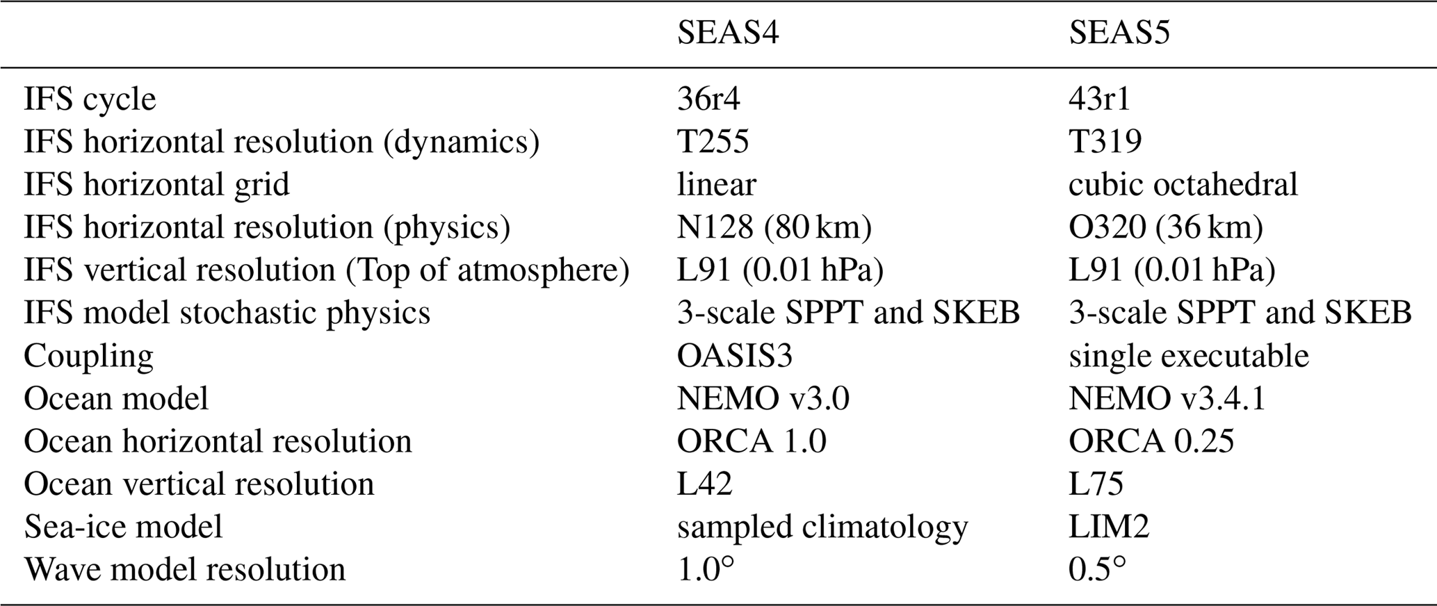
Table 1 summarises the configuration of SEAS5 and compares it to SEAS4. SEAS5 uses updated versions of the atmosphere and ocean models and adds a new interactive sea-ice model, and each of these components are described in detail below.
Table 1Table comparing the configuration of SEAS4 and SEAS5. Abbreviations are defined in the text.
2.2.1 Atmosphere model and forcing
SEAS5 uses ECMWF's IFS atmosphere model cycle 43r1. A brief description of the parameterisations in the IFS is provided here, and the most significant changes between IFS cycle 36r4 (SEAS4) and 43r1 (SEAS5) are highlighted.
The radiation code is based on the Rapid Radiation Transfer Model (RRTM; Mlawer et al., 1997; Iacono et al., 2008). Cloud–radiation interactions are taken into account using the McICA (Monte Carlo Independent Column Approximation) method (Morcrette et al., 2008). For computational efficiency, the radiation calculations are only called every 3 h, which gives a poor representation of the diurnal cycle. In cycle 43r1, this is mitigated by approximate updating at higher time frequency, reducing biases in stratospheric temperature and errors in the diurnal cycle of near-surface temperature (Hogan and Bozzo, 2015; Hogan and Hirahara, 2016).
The parameterisation of convection is based on the mass-flux approach (Tiedtke, 1989; Bechtold et al., 2008). The convective parameterisation evolves with each cycle, and in SEAS5 it has a modified Convective Available Potential Energy (CAPE) closure leading to an improved diurnal cycle of convection (Bechtold et al., 2014) and a revised formulation of detrainment and convective momentum transport improving the tropical flow. The cloud and large-scale precipitation scheme (Tiedtke, 1993; Forbes et al., 2011; Forbes and Tompkins, 2011) has an improved representation of mixed-phase clouds in cycle 43r1 (Forbes and Ahlgrimm, 2014). In addition, there were numerous other improvements to the parameterisation of microphysics, particularly for warm-rain processes (Ahlgrimm and Forbes, 2014), but also ice-phase processes and ice supersaturation. The combination of changes in the cloud and convection schemes between SEAS4 and SEAS5 substantially reduces biases in tropical temperature throughout the troposphere, as will be seen in Sect. 4.2.
The orographic gravity wave drag is parameterised following Lott and Miller (1997) and Beljaars et al. (2004), and the non-orographic gravity wave drag parameterisation is as described in Orr et al. (2010). The turbulent mixing scheme follows the eddy-diffusivity mass-flux (EDMF) framework, with a K-diffusion turbulence closure and a mass-flux component to represent the non-local eddy fluxes in unstable boundary layers (Köhler et al., 2011). In cycle 43r1, the degree of turbulent mixing in stable conditions has been reduced to improve the representation of low-level jets. This change combined with an increase in the orographic drag led to a significantly better representation of the large-scale circulation (Sandu et al., 2014). The representation of near-surface winds was also improved by a revision of the roughness length (Sandu et al., 2011).
The surface-exchange parameterisation is based on a tiled approach (HTESSEL; Viterbo and Beljaars, 1995; Van den Hurk et al., 2000; Balsamo et al., 2009; Dutra et al., 2010a; Boussetta et al., 2013) representing different sub-grid surface types for vegetation, bare soil, snow and open water. The hydrology for soil infiltration and run-off is described by Balsamo et al. (2009) and the representation of surface snow is described in Dutra et al. (2010a). For cycle 43r1, a representation of inland-water bodies that can carry significant thermal storage and anomalies in the forecasts has been introduced (Mironov et al., 2010; Dutra et al., 2010b; Balsamo et al., 2012). In cycle 43r1, the skin temperature for ocean points takes account of the cool skin effect and a diurnal warm layer effect (Zeng and Beljaars, 2005).
SEAS5 was developed following a “seamless” approach, so the atmospheric component of SEAS5 is nearly identical to the IFS cycle 43r1 configuration used for the ENS extended forecast (IFS, 2016), which was operational for medium- and extended-range forecasting from 22 November 2016 to 11 July 2017. The atmospheric model uses a two-time-level semi-Lagrangian scheme, with spectral horizontal resolution of T319 and a 20 min time step. The model physical parameterisations are calculated in physical space on a reduced O320 Gaussian grid, which has a grid spacing of approximately 36 km. There are 91 levels in the vertical, with a model top in the mesosphere at 0.01 hPa or around 80 km. The ECMWF wave model is used at 0.5∘ resolution (IFS, 2016, Part VII) with the same time step as the atmosphere. One change to the cycle 43r1 model settings was introduced for SEAS5. In SEAS5 the tropical amplitude of the non-orographic gravity wave drag was considerably reduced compared to the default settings in cycle 43r1 in order to improve the modelling of the QBO and the climate mean stratospheric winds. The impact of this change is described in Sect. 4.4.
Greenhouse gas radiative forcing consists of a zonally averaged seasonally varying climatology derived from the Monitoring Atmospheric Composition and Climate reanalysis (MACC reanalysis; Inness et al., 2013) which is scaled to capture the long-term trend in greenhouse gas emissions using CMIP5 historical greenhouse gases from 1981 to 2000 and CMIP5 RCP 3-PD from 2000 on as in ERA5. A new prognostic ozone scheme (Monge-Sanz et al., 2011) replaces the scheme used in SEAS4 and the default 43r1 configuration (Cariolle and Déqué, 1986; Cariolle and Teyssèdre, 2007); but as part of the seamless strategy used to develop SEAS5, prognostic ozone is not radiatively interactive as it was in SEAS4. Instead, the radiation scheme sees the same ozone climatology used in the cycle 43r1 ENS extended forecasts. Tropospheric sulfate aerosol follows the decadally varying CMIP5 climatology, rather than the time-invariant climatology that is default in cycle 43r1. Volcanic stratospheric sulfate aerosol is still treated by the method used for SEAS4; the initial load of volcanic aerosol is prescribed using GISS data (2012 update1). The forecast is initialised using the GISS values from the month before the forecast starts, and then evolved in time with damped persistence (timescale 400 days). The vertical distribution follows a prescribed profile that is dependent on the depth of the stratosphere. The horizontal distribution is approximated by three numbers: the Northern Hemisphere, tropical and Southern Hemisphere amounts. SEAS5 cannot predict volcanic eruptions; but after a major eruption occurs, manual estimates of the volcanic aerosol, based in part on the Copernicus Atmosphere Monitoring Service (CAMS) SO2 analyses, could be included in future real-time forecasts. The new prognostic ozone scheme is used to determine the tropopause height for application of volcanic aerosol.
2.2.2 Ocean and cryosphere models
SEAS5 uses the Nucleus for European Modelling of the Ocean model (NEMO, Madec and the NEMO team, 2016) version 3.4.1 developed by the NEMO European consortium, which is an upgrade from the NEMO v3.0 model used in SEAS4. It contains upgrades to aspects of ocean-surface wave interaction (Breivik et al., 2015) originally introduced at ECMWF, including estimating momentum flux from the dissipation term (accounting for the intensity of breaking waves), accounting for the energy flux from breaking waves in surface boundary conditions of the turbulent kinetic energy equation (Craig and Banner, 1994), and introducing the Coriolis–Stokes forcing term in the momentum equation.
The ocean model horizontal resolution increases from ORCA1∘ in SEAS4 to ORCA0.25∘ (developed by the DRAKKAR international research network) in SEAS5, which improves the representation of sharp fronts and ocean transports in SEAS5. The number of ocean vertical levels increases from 42 to 75, including an increase from 5 to 18 levels in the uppermost 50 m of the ocean. This reduces the depth of the surface layer of the ocean model from 10 to 1 m, which improves the representation of the diurnal cycle of SSTs. The ocean model time step is 20 min.
The Louvain-la-Neuve sea-ice model version 2 (LIM2; Fichefet and Maqueda, 1997), developed at the Belgian Université catholique de Louvain, is added in SEAS5. Introducing a prognostic sea-ice model allows the sea-ice cover to respond to changes in the atmosphere and ocean states, enabling SEAS5 to provide seasonal outlooks of sea-ice cover. At the same time, prognostic sea ice has the potential to improve forecasts of the atmospheric state and circulation by virtue of improved surface fluxes of heat, moisture and momentum. LIM2 is part of the NEMO modelling framework and uses the same tripolar ORCA0.25∘ grid as the ocean, but has an hourly time step. It is a dynamic–thermodynamic model with a single thickness category. The model is used within SEAS5 to simulate the evolution of the fractional ice cover (sea-ice concentration), and only this variable is coupled to the atmosphere surface scheme. LIM2 simulates the conductive heat flux within the ice based on two vertical layers in the ice with varying thickness and a single snow layer on top of the ice, which determines the basal ice growth rate during winter. The surface heat flux at the sea-ice–atmosphere interface, however, is determined by an ice conductive heat flux computed by the atmosphere model. This leads to thermodynamic inconsistencies at the surface, resulting in an overestimation of the basal ice growth rate in winter, as seen in Sect. 4.3. The model also does not simulate the formation or evolution of melt ponds, which is important for summer surface energy balance. Ice velocities are computed by solving an appropriate momentum balance equation using a viscous-plastic rheology; sea-ice velocities are important because they give rise to the transport of sea-ice properties by advection.
2.2.3 Coupling
Some of the model components are tightly coupled: the land component, being on the same grid as the atmosphere model and requiring only vertical physics, has always been embedded within the atmosphere model; the ocean and sea-ice components are also tightly coupled to each other. A coupling interface then computes exchanges of information between three distinct modules that use three different horizontal grids: the atmosphere and land, the ocean and sea ice, and the wave model. The atmosphere and wave models exchange fluxes of heat, momentum, freshwater and turbulent kinetic energy with the ocean and sea ice, while the ocean and sea-ice models communicate SST, surface currents and sea-ice concentration to the atmosphere and wave models. There is no coupling between land and ocean.
The coupling interface in SEAS5 is implemented as a single executable, whereas SEAS4 used the OASIS3 coupler (Valcke, 2013). Details on the single executable coupling interface can be found in Mogensen et al. (2012b). As in SEAS4 (Molteni et al., 2011), a Gaussian method is used for interpolation between the atmosphere and ocean models in both directions, primarily due to the complexity of the ORCA0.25∘ grid. The Gaussian method automatically accounts for the different coast lines of the atmosphere and ocean models – values at land points are never used in the coupling since these can be physically very different to conditions over water. The atmosphere and ocean are coupled hourly to allow the diurnal cycle to be resolved.
2.3 Model initialisation
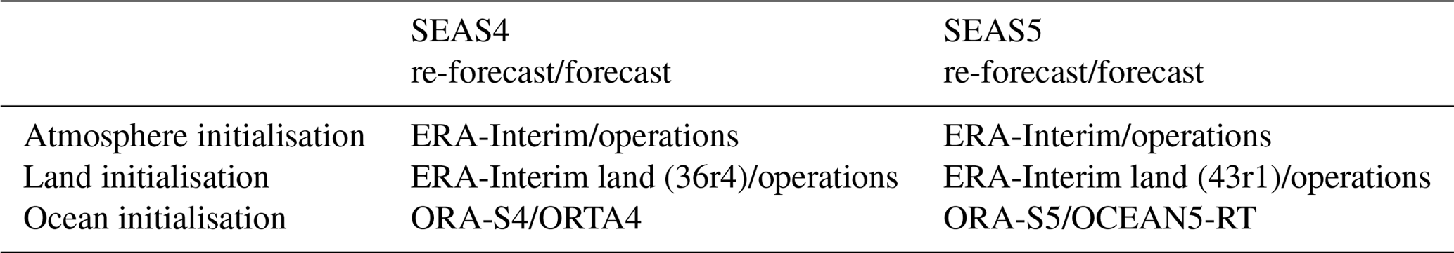
Table 2 summarises the main datasets used to initialise SEAS5 and compares them to those used in SEAS4. The model used to calculate SEAS5 forecasts and re-forecasts is identical, but forecasts must be initialised differently from re-forecasts in order to make use of near-real-time observational data. Forecasts and re-forecasts should be initialised and calculated as similarly as possible to ensure accurate bias correction. We describe the initialisation of both re-forecasts and forecasts here, including any adjustments made to improve consistency between re-forecast and forecast initialisation.
Table 2Table summarising the initialisation of SEAS4 and SEAS5. Abbreviations are defined in the text.
2.3.1 Atmosphere and land
In SEAS5 re-forecasts (prior to 1 January 2017) the atmosphere is initialised from ERA-Interim (Dee et al., 2011). ERA-Interim analysis is not available in time for SEAS5 forecast initialisation, so forecasts (1 January 2017 and later) are initialised from ECMWF operational analyses instead.
The inter-annual variability in ozone in ERA-Interim is affected by changes in satellite instruments over time, and does not represent the true inter-annual variability in ozone in the atmosphere (Dee et al., 2011). Consequently, the prognostic ozone scheme in both re-forecasts and forecasts is initialised with a seasonally varying climatology produced by the ozone model (Monge-Sanz et al., 2011) within an integration where an enhanced vertical resolution version of the IFS (cycle 42r1, L137) is nudged to ERA-Interim vorticity (12 h timescale) and tropopause temperature (5-day timescale, which is needed to control biases in lower stratosphere temperature).
Land-surface initial conditions for the re-forecasts are generated by the cycle 43r1 version of the HTESSEL scheme run in offline mode for the re-forecast period at the same resolution as SEAS5. In offline mode, HTESSEL is forced with ERA-Interim (precipitation, solar radiation, near-surface temperature, winds and humidity) following the method described in Balsamo et al. (2015).
The land surface in SEAS5 forecasts is initialised from ECMWF operational analysis, which includes a dedicated land data assimilation as described in de Rosnay et al. (2014). The SEAS5 land initial conditions are then interpolated from the HRES O1280 grid onto the O320 SEAS5 grid. This interpolation can result in locally large differences compared to initial conditions prepared directly at the lower resolution. Consequently, a limiter is used to prevent the real-time land-surface values taking inconsistent values relative to those used in the re-forecasts. The limits are defined as the maximum and minimum values observed at that point and calendar date for the 36-year re-forecast period, plus an additional margin specified as a global constant for each field. For more details please refer to the SEAS5 user guide2.
2.3.2 Ocean
SEAS5 ocean and sea-ice initial conditions for forecasts and re-forecasts are provided by the new operational ocean analysis system, OCEAN5 (Zuo et al., 2019), which is made up of the historical ocean reanalysis (ORAS5) and the daily real-time ocean analysis (OCEAN5-RT). OCEAN5 uses the same ocean and sea-ice model as the coupled forecasts in SEAS5. OCEAN5 is conducted with NEMOVAR (Mogensen et al., 2012a) in its 3D-Var FGAT (First-guess at appropriate time) configuration. Compared to its predecessor ORAS4 (Balmaseda et al., 2013), OCEAN5 has higher resolution, updated data assimilation and observational datasets, and provides sea-ice initial conditions.
ORAS5 is based on Ocean Reanalysis Pilot 5 (ORAP5; see Zuo et al., 2017b; Tietsche et al., 2017), but using updated observational datasets. The ocean in situ temperature and salinity comes from the recent quality-controlled EN4 (Good et al., 2013), which has higher vertical resolution and better spatial coverage than the previous version EN3. The altimeter sea-level data have also been updated to the latest version (AVISO DT2014, Pujol et al., 2016) from CMEMS (Copernicus Marine Environmental Monitoring Services). The underlying SST analysis before 2008 comes from the HadISSTv2 dataset (Titchner and Rayner, 2014), which was the historical SST dataset most consistent with the Operational Sea Surface Temperature and Sea Ice Analysis (OSTIA) SST product used in operations at ECMWF. The sea-ice concentration comes from ERA-40 before 1985 and from an OSTIA (Donlon et al., 2012) reprocessed product between 1985 and 2008. From 2008 onwards both SST and sea-ice concentration are given by the OSTIA operational product, which is the same as used in the ECMWF operational atmospheric analysis. Further details of the OCEAN5 configuration and its sensitivities are discussed in Zuo et al. (2019).
2.4 Ensemble generation
2.4.1 Initial condition perturbations
Initial condition perturbations are applied to atmosphere and ocean initial conditions to represent uncertainty in the initial state and increase ensemble spread. Ensemble member 0 is initialised from unperturbed atmospheric initial conditions; in other members all upper air fields and a limited set of land fields (soil moisture, soil temperature, snow, sea-ice temperature and skin temperature) are perturbed. As in the operational ENS, perturbations from an ensemble of data assimilations (EDA) and perturbations constructed from the leading singular vectors are applied (IFS, 2016, Part V). EDA perturbations are only available for the later years in the re-forecast set; so to preserve consistency across the hindcast set and forecasts, the EDA perturbations from 2015 were applied to the initial conditions for all forecast and re-forecast years. The EDA perturbations are new in SEAS5, while singular vector perturbations were also used in SEAS4 with settings from IFS cycle 36r4.
OCEAN5 contains a 5-member ensemble analysis. The perturbation scheme used to generate this ensemble consists of two distinct elements: perturbations to the assimilated observations, both at the surface and at depth, and perturbations to the surface forcing fields. The forcing perturbations used to generate the ocean re-analyses are monthly realisations of SST errors, wind stress, solar radiation and fresh water flux sampling analysis error, as described in Zuo et al. (2017a). While monthly perturbations are used to create the analysis ensemble, pentad perturbations of SST from HadISSTv2 are used to further augment the number of initial ocean conditions. First, each SEAS5 ensemble member is assigned one of the OCEAN5 ensemble members: OCEAN5 member 0 for SEAS5 member 0 counting up to OCEAN5 member 4 for SEAS5 member 4, and starting again at OCEAN5 member 0 for SEAS5 member 5. Then further perturbations, drawn from the HadISSTv2 pentad analysis error repository and unique to each ensemble member (Zuo et al., 2017a, Section 4), are applied to the upper 22 levels of the ocean temperature, decreasing with depth. This perturbation is not applied to ensemble member 0. The pentad perturbations applied to the forecast initial conditions sample the fast analysis error, while the monthly perturbations applied to the ocean re-analyses sample errors with longer (1-month) decorrelation timescales. There are several differences between ocean initial condition perturbations in SEAS4 and SEAS5, the main differences are in the perturbation repository and the introduction of two temporal decorrelation scales; for details, see Zuo et al. (2017a).
2.4.2 Stochastic model perturbations
In addition to perturbing the initial conditions, perturbations to the atmospheric model are applied to represent uncertainty from missing or unresolved sub-grid-scale processes (e.g. convection, clouds, radiation, turbulence) which have to be parameterised (Palmer, 2012). ECMWF has been using stochastic parameterisation schemes to explicitly account for these uncertainties in its forecasting systems from the medium-range to seasonal forecasts for many years (Buizza et al., 1999; Palmer et al., 2009) and the schemes that are used in SEAS5 are identical to those used in the shorter forecast ranges in cycle 43r1 (see Leutbecher et al., 2017). The stochastically perturbed physical tendency (SPPT) scheme introduces flow-dependent multiplicative noise to the total tendencies of the prognostic variables temperature, horizontal wind and humidity at model levels. The noise has a spatial and temporal correlation structure with three distinct scales representing small-scale fast perturbations, large-scale slow perturbations and an intermediate scale. A tapering in the boundary layer and the upper-most model levels effectively switches off the SPPT perturbations in these regions. The version of SPPT used here is based on a mass, energy and moisture conservation fix that was originally developed by the EC-Earth consortium (see Lang et al., 2016). The stochastic kinetic energy backscatter (SKEB) scheme aims at improving the upscale energy cascade from the sub-grid scales to the resolved scales (Shutts, 2005), but has been found to have a smaller overall impact in the ECMWF system (Weisheimer et al., 2014). Both of these schemes were also used in SEAS4, with settings from IFS cycle 36r4. For details of the schemes and performances, see Palmer et al. (2009), Lang et al. (2016), Leutbecher et al. (2017) and Weisheimer et al. (2014). Stochastic perturbations from both SPPT and SKEB are applied to all ensemble members; SEAS5 does not have a control forecast.
In order to compare the SEAS5 skill with the previous operational system (SEAS4), we could work with the largest common period for which the re-forecasts from SEAS4 and SEAS5 are available (namely 1981 to 2010). Since a key component of the seasonal forecast skill is the ability to forecast ENSO, it is important to consider a long verification period to include sufficient numbers of ENSO events. To allow a longer verification period we have included the operational forecasts for SEAS4 for 2011 to 2016, giving an overall comparison period of 1981 to 2016. This choice is not perfect since there are inconsistencies in the land-surface initialisation between the SEAS4 re-forecasts and SEAS4 real-time forecasts. Comparison of the SEAS5 and SEAS4 score differences for 1981 to 2010 and 1981 to 2016 (not discussed in this paper) shows no sign of this slight inconsistency affecting the results presented here. Consequently, the assessment in this paper is based on this 36-year re-forecast period unless otherwise mentioned (see Sect. 3.2), which is consistent with the SEAS5 verification available on the ECMWF website3.
SEAS5 has an increased operational re-forecast ensemble size compared to SEAS4; however, the real-time ensemble size is the same in both systems. Since we are interested in the comparative skill of the real-time forecast system, throughout this article we compare the two forecast systems using the same ensemble size. Since the implementation of SEAS4, extra ensemble members have been added to quarterly re-forecast dates (February, May, August, November), allowing us to compare the 25-member SEAS5 re-forecast set to 25 ensemble members from SEAS4. When only 15 SEAS4 ensemble members are available, we compare them to the first 15 members from SEAS5.
Our assessment is performed on monthly means. “Forecast lead time” is defined here to be the months elapsed since forecast initialisation but prior to the month being discussed, while “forecast month” includes the month being discussed, one more than forecast lead. For example, if a forecast is initialised on 1 January, February has 1-month forecast lead time and is month 2 of the forecast.“Verification month” is defined as the calendar month that the forecast is issued for. Unless otherwise mentioned, diagnostics are seasonal means at 1-month lead time (i.e. a DJF SST map is from a 1 November start date), which corresponds to months 2 to 4 of the forecast.
3.1 Evaluation and verification metrics
The seasonal forecast performance has been evaluated using a wide range of deterministic and probabilistic scores. For ENSO forecasts and other SST statistics we use deterministic metrics such as anomaly correlation and root mean square error. For the skill of atmospheric variables we also use probabilistic metrics such as the continuous ranked probability score and reliability diagrams.
3.1.1 Anomaly correlation
Anomaly correlations are calculated in accordance with established practice for scoring ENSO forecasts. First, bias-corrected anomalies for each forecast date and lead time in the re-forecast dataset are created using cross validation (i.e. the bias correction is calculated only from other re-forecast years, not the one being bias corrected). Anomalies for tropical ocean indices are calculated with respect to a standard 30-year reference climate period, which is 1981 to 2010. All other anomalies are calculated with reference to the full validation period of 1981 to 2016. The correlation is then calculated between the ensemble mean forecast and observed anomaly time series. The cross-validation procedure affects the correlation negatively, leading in theory to a small but systematic underestimate of expected future forecast skill.
3.1.2 Amplitude ratio
The ratio of the forecast anomaly amplitudes to observed amplitudes is calculated from the cross-validated bias-corrected individual ensemble member anomalies, computed with respect to 1981 to 2010. The standard deviation of the forecast anomalies is calculated from the mean square amplitude of all ensemble members and all start years (for a given start month and lead time), and then compared with the standard deviation of observations.
3.1.3 Root mean square error
For tropical ocean and QBO indices, the root mean square error (RMSE) is calculated from the cross-validated bias-corrected ensemble mean of the forecasts.
3.1.4 CRPSS
The continuous ranked probability skill score (CRPSS; Wilks, 2011) is calculated for each variable's seasonal average at each grid point for each year of the whole re-forecast period. It follows that the CRPSS map is estimated over 36 independent events. A climatology computed over the 36-year re-forecast period is used as the reference forecast. Therefore the CRPSS gives an indication of the added value of a forecasting system over simply forecasting climatology: a value of 1 indicating perfect forecasts, 0 showing no improvement over climatology and negative values indicating a failing forecasting system. Significance testing for the CRPSS differences between SEAS5 and SEAS4 is evaluated at a 5 % significance level with a Z test on pairwise bootstrapped CRPSS differences. For this Gaussian-approximated bootstrap method, we resample the forecasts and ensemble members over 1000 repetitions (with replacement) to capture the uncertainty both in time and in the ensemble.
3.1.5 Reliability
Reliability diagrams are used to summarise whether the forecast probabilities agree with the observed frequency of occurrence of a binary event (e.g. temperature in the upper tercile). To create the reliability diagrams used in this paper, each forecast at every grid point within a selected region is binned into 1 of 26 bins (one more than the number of ensemble members) according to the forecasted likelihood of occurrence of the chosen event. This likelihood is then plotted against the frequency with which the event actually occurred for this subset of forecasts and grid points. In a perfectly reliable system, the forecast probability will equal the frequency of occurrence and the values for each bin will lie along a straight diagonal line in the reliability diagram. Uncertainties are computed by bootstrapped resampling over years and ensemble members.
3.2 Datasets
For most variables the ERA-Interim reanalysis was used for verification (Dee et al., 2011), which is also the atmosphere initialisation data for SEAS4 and SEAS5. To verify precipitation we use the Global Precipitation Climatology Project (GPCP) monthly precipitation analysis 2.2 (Adler et al., 2003). Since GPCP 2.2 data are not available for the whole re-forecast period, precipitation verification statistics are based on the 1981 to 2014 period.
The depth of the surface layer of the ocean model decreases from 10 m in SEAS4 to 1 m in SEAS5, which changes the depth that SST is calculated from. To ameliorate the impact of this difference on the SST biases, we initially compare SST maps in each system to the analysis it was initialised from, ORAS4 (Balmaseda et al., 2013) or ORAS5 (Zuo et al., 2019). Later, area-averaged SST indices are compared to the OI.v2 reanalysis (OIv2; Reynolds et al., 2002), or ERA-Interim reanalysis, to measure both systems against the same standard. As will be seen in Sect. 4, when averaging over large regions, consistent conclusions are reached regardless of which observational dataset is used.
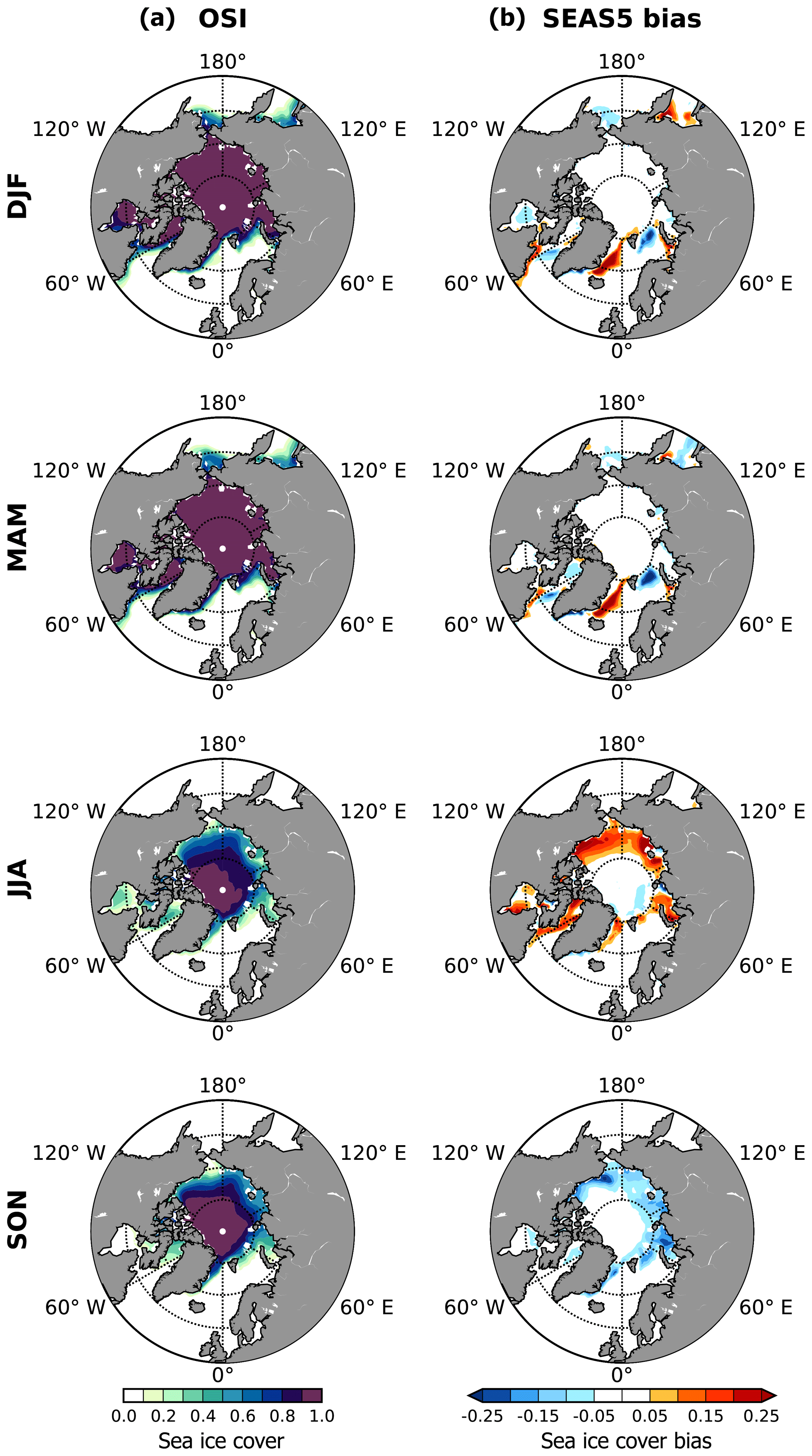
ERA-Interim sea ice is not temporally consistent, and is not recommended as a sea-ice verification dataset. Instead, we use the EUMETSAT Ocean and Sea Ice Satellite Application Facilities' (OSI SAF) global sea-ice concentration climate data record (OSI-450)4. OSI-450 is the second major version of the OSI SAF Global Sea Ice Concentration Climate Data Record. The sea-ice concentration is computed from the SMMR (1979–1987), SSM/I (1987–2008) and SSMIS (2006–2015) instruments. The OSI-450 product is available from 1979 to 2015; but because of gaps in the satellite record, data are not available for every day. We have taken the choice that if five consecutive days of data are missing from any season, that season is left out of our evaluation of sea-ice concentration. Consequently, in JJA we exclude 1984, 1986 and 2016; in DJF we exclude 1986, 1987, 1990, 2015 and 2016; in MAM we exclude 1981, 1986 and 2016; and in SON we exclude 2016.
In this section we use diagnostics of inter-annual processes to assess SEAS5 and compare it to SEAS4. We first discuss the tropics, with a focus on tropical SST variability (Sect. 4.1). Then we discuss the northern extratropics, with a particular focus on the North Atlantic SST (Sect. 4.2). Finally we discuss the impact of introducing the prognostic sea-ice model LIM2 (Sect. 4.3) and the representation of the stratosphere (Sect. 4.4), before going on to discuss the global verification of SEAS5 in the next section.

Figure 1DJF and JJA SST bias in the tropics at 1-month forecast lead for SEAS4 (a, b) and SEAS5 (c, d) compared to the analysis they were initialised from (ORAS4, ORAS5). The regions discussed in detail later in this section are outlined in grey here.
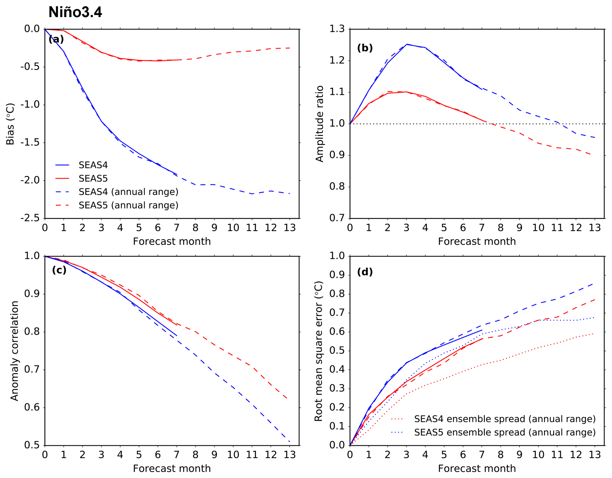
Figure 2Forecast performance metrics (described in Sect. 3.1) of the monthly averaged Niño 3.4 index in SEAS4 (blue) and SEAS5 (red). Long-range (7-month) forecasts are shown as the solid lines, and use 15 ensemble members from each of the 12 monthly start dates. Annual-range (13-month) forecasts are shown as the dashed lines, and use 15 ensemble members from each of the four quarterly start dates. The verification data are NCEP OIv2. The top row shows (a) climatological bias and (b) ratio of the standard deviation of re-forecast and OIv2 anomalies, calculated using individual ensemble members. The bottom row shows (c) anomaly correlation and (d) RMSE (solid and dashed lines) and ensemble spread (dotted lines).
4.1 Tropics
Inter-annual modes of variability in tropical oceans are the primary known source of seasonal predictability (e.g. Charney and Shukla, 1981; Palmer and Anderson, 1994; Stockdale et al., 1998; Troccoli, 2010). Consequently, a realistic representation of the tropical variability is a crucial requirement for a successful seasonal forecasting system. In Fig. 1, we show the tropical SST bias in SEAS4 and SEAS5 relative to the ocean reanalysis they were initialised from ORAS4 or ORAS5 (see Sect. 3.2). The tropical oceans are generally warmer in SEAS5, especially in the summer hemisphere. This overall warming is mainly due to changes in the ocean vertical mixing, which produces shallower mixed layers within the tropical regions. Warm biases flank the Equator in the tropical Pacific and Atlantic basins. In the Indian Ocean and west Pacific, cold biases in SEAS4 are replaced with a warm bias in SEAS5. There is a reduction in the equatorial Pacific cold tongue bias in SEAS5 that exceeds 5 ∘C at its maximum in SEAS4. Initial investigations suggest that both the increase in ocean model horizontal resolution and improvements in the atmosphere model contribute to the reduction of the cold tongue bias. Improvements in IFS tropical convection and cloud physics give higher total column water vapour in SEAS5, with more absorption of thermal radiation, resulting in a reduction in tropical outgoing long-wave radiation of 3.0 W m−2 in DJF and 2.4 W m−2 in JJA. This change to the atmosphere radiative balance may contribute to the changes in tropical SST.

Figure 3Forecast performance metrics of the monthly averaged Niño 3.4 index in SEAS4 (blue) and SEAS5 (red) as a function of verification month. The solid lines are averaged over 1 to 3 months lead times, and the dashed lines are averaged over 4 to 6 months lead times. Each line uses 15 ensemble members. The top row shows (a) Niño 3.4 SST climatological bias and (b) ratio of the standard deviation of the re-forecast and OIv2 anomalies, calculated using the individual ensemble members. The bottom row shows (c) anomaly correlation and (d) RMSE. The standard deviation of the inter-annual variability in OIv2, indicating the annual cycle of the inter-annual variability, is plotted as the dotted line in panel (d).
The dominant mode of global SST inter-annual variability is the ENSO (e.g. McPhaden et al., 2006; Deser et al., 2010). Figure 2 shows the mean state bias, amplitude ratio, anomaly correlation and RMSE of the Niño 3.4 region (5∘ N to 5∘ S, 120 to 170∘ W; illustrated in Fig. 1) as a function of forecast lead time using 15 ensemble members from all start dates of the SEAS4 and SEAS5 hindcast set. For a detailed description of these metrics see Sect. 3.1. In order to compare the systems on an equal footing, these diagnostics are computed relative to the NCEP OIv2 reanalysis (see Sect. 3.2). Both the long-range forecast (solid lines) and annual-range forecast (dashed lines) are shown for SEAS4 and SEAS5 (see Sect. 2.1).
The decrease in the equatorial Pacific cold tongue bias seen in Fig. 1 is also clear in Fig. 2, with an improvement of nearly 2∘ in the SEAS5 Niño 3.4 bias after 13 months of model evolution. The SEAS5 bias does not change very much after the first few months of the forecast, while the SEAS4 bias continues to grow through the early parts of the annual-range forecast. The other metrics in Fig. 2 reveal that the inter-annual variability in ENSO has also improved. For the 7-month duration of the long-range forecast in both SEAS4 and SEAS5, the amplitude of the variability exceeds that of the analysis indicating the model is overactive in the equatorial Pacific. This overactivity is reduced in SEAS5, with an approximately 10 % improvement in the amplitude ratio in the long-range forecast. ECMWF already had high skill in forecasting ENSO compared to other state-of-the-art seasonal forecast models, especially in the boreal spring and summer months that are more difficult to forecast (Barnston et al., 2012; Molteni et al., 2011). This skill is improved in SEAS5, with an improved anomaly correlation at all lead times, but particularly in the annual-range forecast. These improvements combine to improve RMSE by approximately 0.1 ∘C at forecast leads longer than 1 month. Improvements in ENSO skill are particularly noticeable in the western-central Pacific (e.g. Niño 4), while they are more modest in the eastern part of the basin (e.g. Niño 3) (not shown). In spite of these improvements, SEAS5 continues to be under-dispersive in the ENSO regions, the ensemble spread is approximately 80 % of the RMSE at lead times longer than 1 month, as shown by the dotted lines in Fig. 2d. SEAS5 is slightly more under-dispersive than SEAS4, due to a larger drop in the spread than improvement in the skill in the Niño 3 region (not shown).
Table 3Niño 3.4 anomaly correlation values for the annual-range forecast using the ensemble mean of 15 ensemble members, listed as a function of lead time (months) for two verifying months (January and July).
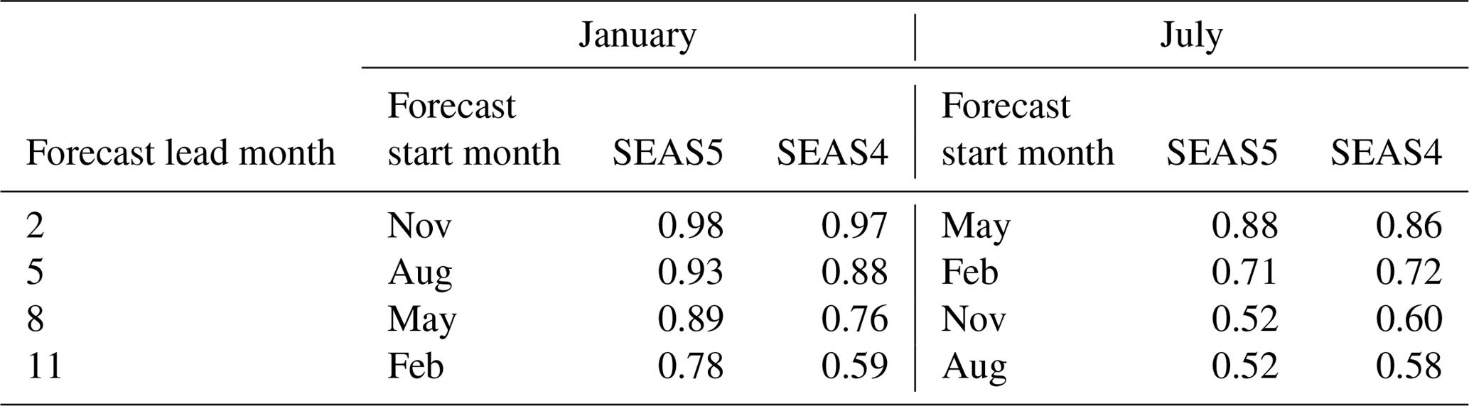
SEAS5 ENSO forecast skill, like ENSO anomalies themselves, varies throughout the year. In Fig. 3 we show the same four metrics that were depicted in Fig. 2, but as a function of verification month. The solid lines are averaged over lead times of 1 to 3 months, and the dashed lines are averaged over lead times of 4 to 6 months. Here we can see that while the Niño 3.4 bias improves throughout the year, it is particularly improved in late JJA and SON at longer lead times. In SEAS5, the bias is fairly consistent throughout the year, though it is a bit larger in spring at longer lead times. In both SEAS5 and SEAS4, the model is particularly overactive in MAM, and this overactivity grows at longer lead times, whereas in SON and DJF overactivity diminishes at longer lead times. The anomaly correlation decreases at longer lead times, as expected, but particularly in JJA and early SON. This is also seen in the annual-range forecast. In Table 3 we show the anomaly correlation for Niño 3.4 January and July anomalies at forecast leads of 2, 5, 8 and 11 months. SEAS5 January skill is maintained well throughout the forecast, with an anomaly correlation of 0.78 at 11 months forecast lead. In SEAS4 this dropped to 0.59. This represents a considerable improvement in the ENSO prediction skill of the annual-range forecast. In JJA, when Niño 3.4 anomalies are generally smaller, the anomaly correlation in both systems has dropped below 0.6 by 8 months forecast lead and SEAS4 outperforms SEAS5 by a small margin.
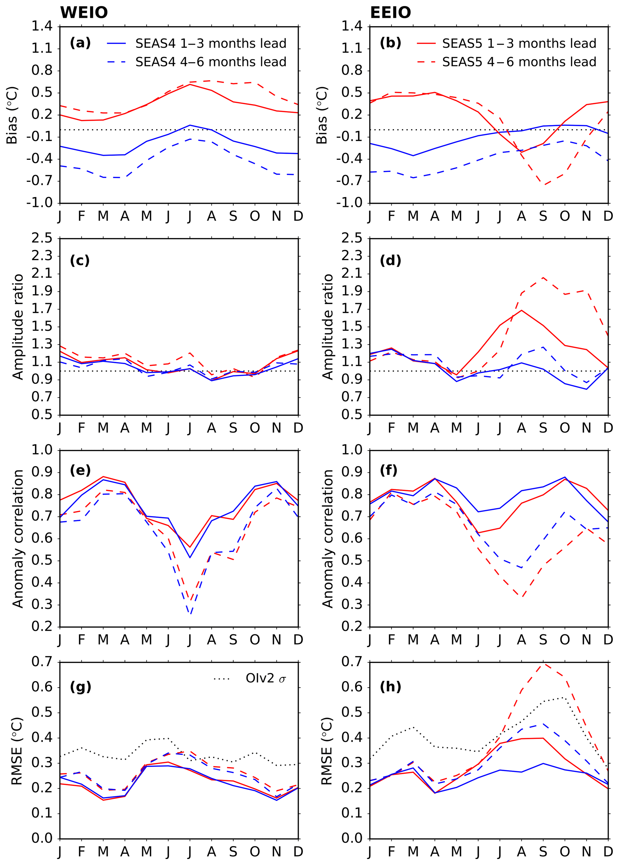
Figure 4Forecast performance metrics of the regions that contribute to the Indian Ocean Dipole index (illustrated in Figure 1) as a function of verification month; (a, b) SST climatological bias; (c, d) Ratio of the standard deviation of forecast and OIv2 anomalies; (e, f) Anomaly correlation; (g, h) RMSE. SEAS4 is shown in blue and SEAS5 is shown in red. The solid lines are averaged over 1 to 3 months lead times, and the dashed lines are averaged over 4 to 6 months lead times. Each line uses 15 ensemble members. The standard deviation of the inter-annual variability in OIv2, indicating the annual cycle of the inter-annual variability, is plotted as the dotted line in panels (g) and (h).
Other important modes of tropical SST variability include the Indian Ocean Dipole (IOD; Saji et al., 1999; Webster et al., 1999) and tropical Atlantic variability sometimes referred to as the Atlantic Niño (e.g. Zebiak, 1993). Figure 4 shows metrics as a function of verification month for the regions that form the IOD index: the western equatorial Indian Ocean (WEIO; 10∘ N to 10∘ S, 50 to 70∘ E) and eastern equatorial Indian Ocean (EEIO; 0 to 10∘ S, 90 to 110∘ E). These regions are illustrated as grey boxes on the maps in Fig. 1. In the WEIO, a cold bias in SEAS4 becomes a warm bias in SEAS5, but the amplitude of the bias remains similar. Otherwise, very little changes from SEAS4 to SEAS5. The anomaly correlation shows some variation with season in both systems, with a particular drop in anomaly correlation in July. In the EEIO, SEAS5 metrics degrade compared to SEAS4, and there is clear seasonality to this degradation. In a positive IOD event, a cold anomaly develops in the EEIO off the coast of Sumatra. In SEAS5, these cold events develop most years, and with large amplitudes, likely related to a deficit in precipitation in the EEIO and an easterly wind bias (not shown). The cold events are visible in Fig. 4b and d, where the bias is cold in the EEIO from July through autumn (depending on lead time) and the amplitude of the variability is much too large, nearly double the observed amplitude at longer lead times. This has a marked detrimental effect on the anomaly correlation and RMSE at longer lead times from July to November.
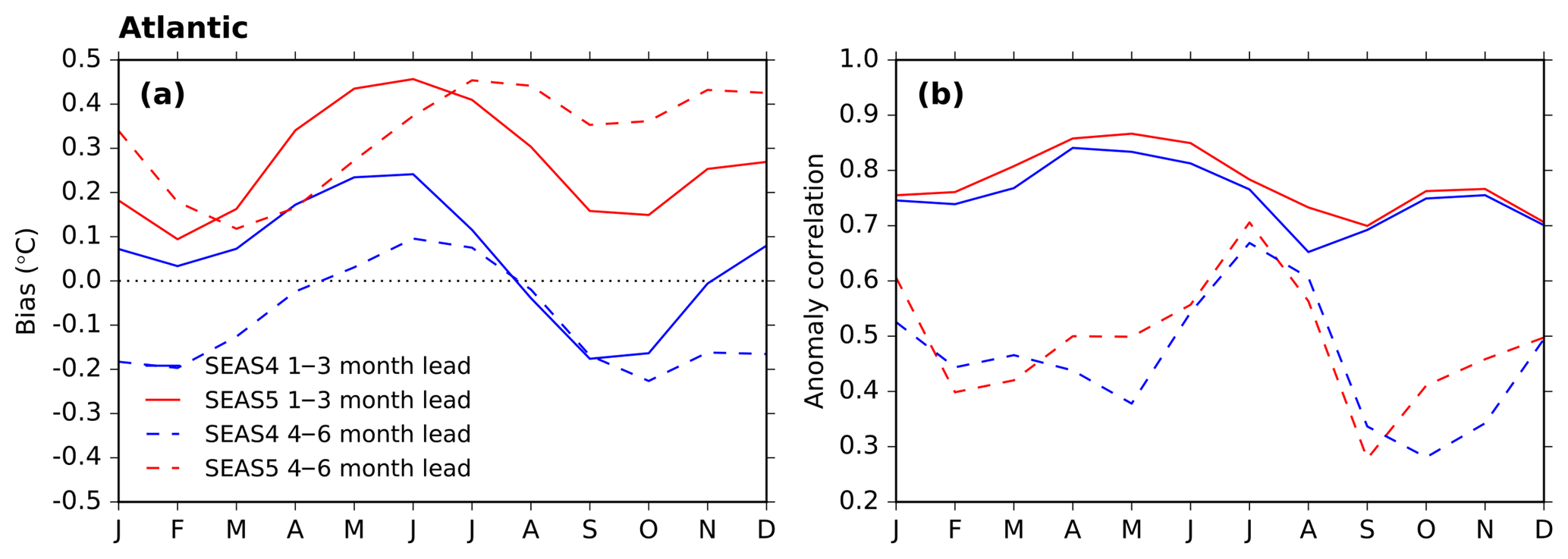
Figure 5Forecast performance metrics for the tropical Atlantic region (illustrated in Fig. 1) as a function of verification month. (a) SST climatological bias and (b) anomaly correlation. SEAS4 is shown in blue and SEAS5 is shown in red. The solid lines are averaged over 1 to 3 months lead times, and the dashed lines are averaged over 4 to 6 months lead times. Each line uses 15 ensemble members.
In Fig. 5 we show the bias and anomaly correlation for the equatorial Atlantic (5∘ N to 20∘ S, 60∘ W to 20∘ E; region illustrated in Fig. 1). In the Atlantic, the SEAS5 bias is warmer and larger throughout the year compared to SEAS4. The amplitude of the inter-annual variability changes very little from SEAS4 to SEAS5 (not shown), but anomaly correlation increases slightly (Fig. 5b), leading to slight decreases in RMSE (not shown). In both systems, skill in JJA, when Atlantic Niño variability peaks (Zebiak, 1993), is maintained through longer lead times, while it degrades at other times of the year.
4.2 Northern extratropics

Figure 6DJF and JJA SST bias in the northern extratropics at 1 month forecast lead for SEAS4 (a, b) and SEAS5 (c, d) compared to the analysis they were initialised from (ORAS4, ORAS5). The region discussed in detail later in Sect 4.2 is outlined in grey here.
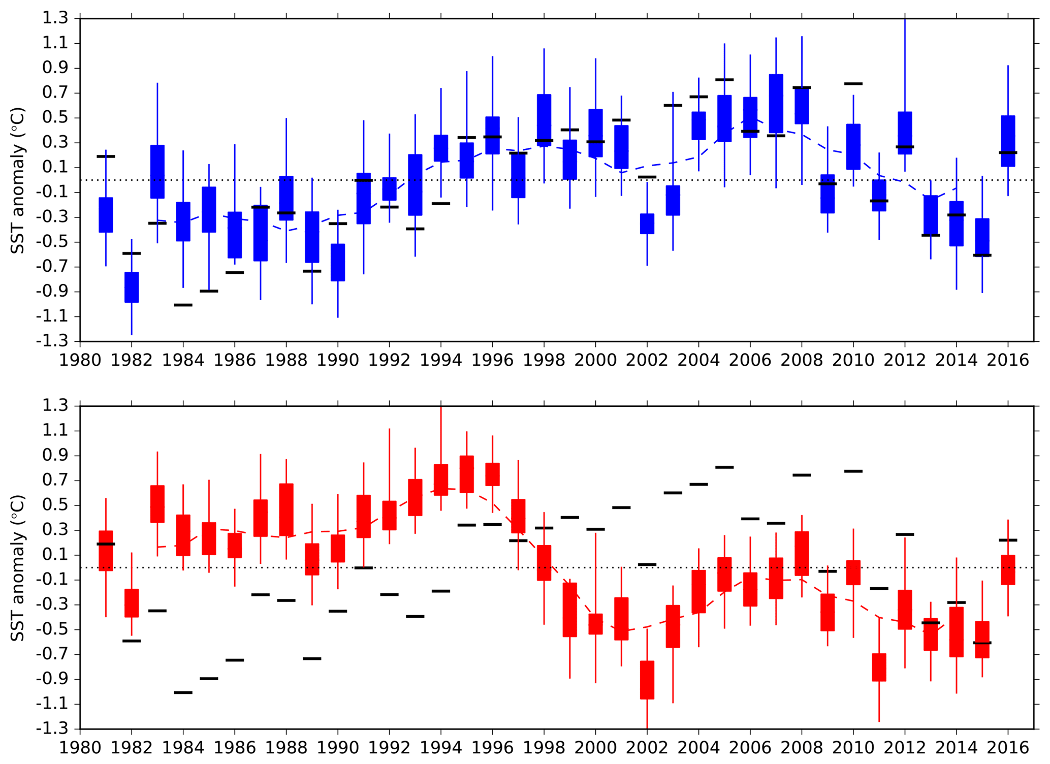
Figure 7DJF time series of SST anomaly in a northwest Atlantic region: 40 to 60∘ N, 50 to 30∘ W (illustrated as a grey box in Fig. 6) at 1 month forecast lead. Quartiles, minimum and maximum of the SEAS4 25-member ensemble are shown in blue, while the SEAS5 25-member ensemble is shown in red. The black bars indicate ERA-Interim reanalysis. A 5-year running mean for each system is shown as a dashed line. Forecasts were initialised in November, and the year shown is the year the ensemble was initialised.
The SST bias in the northern extratropics is shown for both DJF and JJA in Fig. 6. In the northern Pacific, SST biases reduce, particularly in JJA. This is partly due to improved parameterisations for ocean vertical mixing. In the northern Atlantic, increased horizontal resolution in the ocean model alters the path of the Gulf Stream, which changes SST biases. A positive SST bias in the Gulf Stream region is present in both SEAS4 and SEAS5. This is connected to the long-standing and well-known failure of low-resolution ocean models to simulate the separation of the Gulf Stream from the North American coast correctly (Chassignet and Marshall, 2008). This bias has improved in SEAS5. Further downstream, the Gulf Stream meets with the cold Newfoundland Current coming from the north, and splits into the North Atlantic subtropical gyre and the North Atlantic Drift. In this region, marked with the grey box in Fig. 6, the bias changes sign compared to SEAS4. This region is characterised by complex interactions of several large-scale ocean currents that are key to the North Atlantic ocean circulation (Buckley and Marshall, 2016). As will be seen in Sect. 5, SEAS5 also has reduced skill in this region compared to SEAS4.
To investigate the changes in this region, in Fig. 7, we show a time series of the mean SST anomaly in the region highlighted by the grey box in Fig. 6 (40 to 60∘ N, 50 to 30∘ W). In ERA-Interim, the North Atlantic exhibits clear decadal variability: generally cold anomalies in the 1980s, warm anomalies in the 1990s and 2000s, and cold anomalies after 2010. SEAS4 captures this variability, showing the transition from cold to warm anomalies in the mid-1990s, while SEAS5 does not show this variability, leading to a much lower anomaly correlation with respect to ERA-Interim in SEAS5 (−0.1) than in SEAS4 (0.8). Initial investigations suggest that this degradation is caused by the new ocean initial conditions (ORAS5), and is related to the increased horizontal resolution of the ocean analysis system. The deterioration of skill in this region can potentially affect forecasts over Europe through advection by the prevailing westerly winds. Studies further investigating the source and impact of this error are underway, and their results will be discussed in future publications.

Figure 8ERA-Interim zonally averaged profiles of temperature (colours) and zonal wind (contours) for DJF (a) and JJA (b), as well as the biases of SEAS4 (c, d) and SEAS5 (e, f) at 1 month forecast lead.
To analyse changes in the extratropical atmosphere mean state, we first examine the zonally averaged temperature and wind profiles. Figure 8 shows the bias with respect to ERA-Interim in SEAS4 (Fig. 8c, d) and SEAS5 (Fig. 8e, f) for both DJF and JJA. The temperature profile is shown in the colours, while the zonal wind profile bias is overlayed as contours. Improvements in model physics (see Sect. 2.2) have warmed the troposphere in SEAS5, which translates into a clear decrease in the bias in DJF; but in JJA the SEAS5 troposphere is too warm. The tropospheric warming from approximately 30 to 40∘ N degrades the JJA temperature gradients in SEAS5, and coincides with increased errors in the subtropical jets. The SEAS5 jets are too strong at the tropopause level in both seasons, but in JJA errors extend to lower levels and the jets are also positioned too far to the north in both hemispheres. Cold biases at the tropopause worsen in SEAS5, due in part to the increase in horizontal resolution in SEAS5 and in part to humidity errors at the tropopause (Polichtchouk et al., 2017; Shepherd et al., 2018).
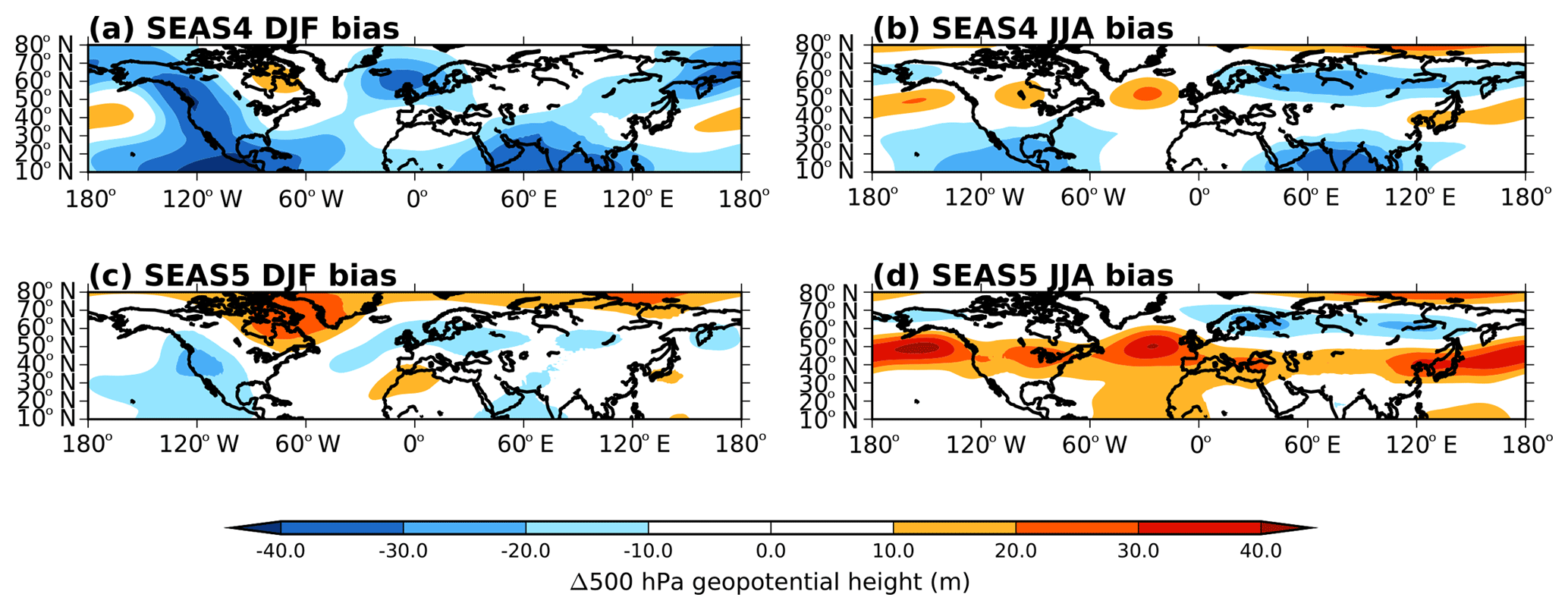
Figure 9Northern extratropics DJF and JJA 500 hPa geopotential height bias with respect to ERA-Interim in SEAS4 (a, b) and SEAS5 (c, d) at 1 month forecast lead.
To examine the spatial structure of these biases, in Fig. 9 we show a map of 500 hPa geopotential height biases relative to ERA-Interim in the northern extratropics. The warming of the troposphere in SEAS5 is reflected in higher geopotential heights in SEAS5, and in DJF this substantially reduces the bias. In JJA, the displacement of the jet shown in Fig. 8 is clearly visible in SEAS5, but also present to a lesser extent in SEAS4.
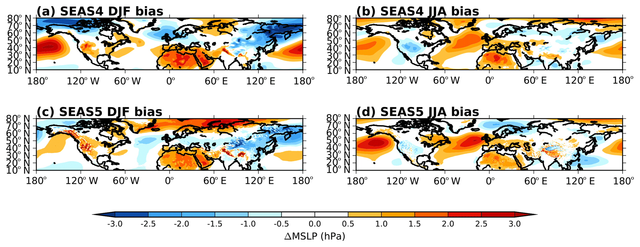
Figure 10Northern extratropics DJF and JJA mean sea level pressure (MSLP) bias with respect to ERA-Interim in SEAS4 (a, b) and SEAS5 (c, d) at 1 month forecast lead.
Many of these bias patterns continue to the surface, as shown in a map of mean sea level pressure (MSLP) biases in Fig. 10. In JJA, SEAS5 high MSLP biases correspond to 500 hPa geopotential height biases in the northern Pacific and Atlantic. In DJF, SEAS5 shows particular improvement (approximately 3 hPa) in the North Pacific subtropical high. There are also improvements in the DJF MSLP trough that centred over the British Isles in SEAS4; however, this is replaced with a bias that projects onto a negative North Atlantic Oscillation (NAO) pattern, reducing the gradient between the NAO centres of action. This may affect whether NAO events have the correct impact.
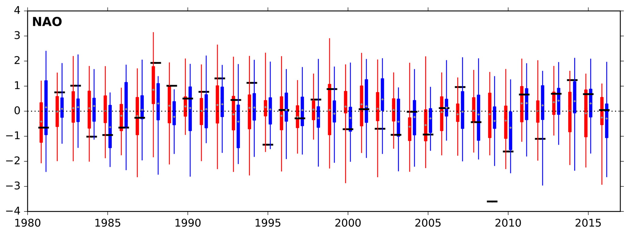
Figure 11Time series of a DJF NAO index derived from projecting the re-forecast 500 hPa geopotential height onto the first EOF of ERA-Interim DJF 500 hPa geopotential height in the North Atlantic. Quartiles, minimum and maximum of the SEAS4 25-member ensemble are shown in blue, while the SEAS5 25-member ensemble is shown in red and ERA-Interim reanalysis is shown in the black bars. Forecasts were initialised in November, and the year shown is the year the ensemble was initialised. The grey diamonds indicate the ensemble mean. Anomaly correlation values for the ensemble mean are 0.46 for SEAS4 and 0.43 for SEAS5. The 95 % confidence interval for sampling error over years is 0.12 to 0.67 for SEAS5.
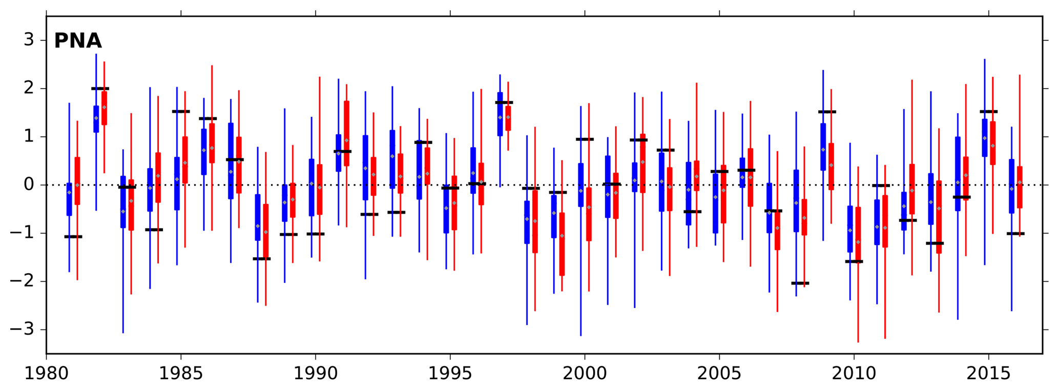
Figure 12As in Fig. 11, but for a PNA index. Anomaly correlation values for the ensemble mean are 0.69 for both systems. The 95 % confidence interval for sampling error over years for SEAS5 is 0.47 to 0.83.
While the extratropics are less predictable on seasonal timescales than the tropics, it is common to analyse the performance of a seasonal forecast system in predicting circulation patterns such as the NAO and the Pacific–North American teleconnection pattern (PNA). In Fig. 11, we show a standardised time series of a DJF NAO index using 25 ensemble members from SEAS4 and SEAS5, calculated by projecting DJF 500 hPa geopotential height onto the first empirical orthogonal function (EOF) of ERA-Interim DJF 500 hPa geopotential height in the North Atlantic (30 to 88.5∘ N, 80∘ W to 40∘ E; Wallace and Gutzler, 1981)5. We see little difference between SEAS4 and SEAS5: both show moderate skill with an anomaly correlation of 0.43 in SEAS5 and 0.46 in SEAS4. Average ensemble spread (standard deviation) has similarly not changed between SEAS4 and SEAS5. Following Dunstone et al. (2016), we also calculated the NAO index as the MSLP difference between two small regions in the North Atlantic (Iceland: 63 to 70∘ N, 25 to 20∘ W and Azores: 36 to 40∘ N, 28 to 20∘ W) where we obtain an anomaly correlation of 0.30 in SEAS5 and 0.39 in SEAS4. This suggests the NAO in the ECMWF model may be less well represented at the surface and is also a reminder that statistics of the NAO are sensitive to which diagnostic is used, how it is calculated and which months and years are used in the calculation. For example, the confidence interval for sampling error over years is 0.12 to 0.67 for SEAS5. The errors in decadal variability in the northwest Atlantic discussed earlier may have a downstream impact on NAO skill in SEAS5; investigations are ongoing.
We show a standardised time series of the PNA teleconnection index in Fig. 12, derived by projecting the DJF 500 hPa geopotential height onto first EOF of ERA-Interim geopotential height in a region covering North America and the North Pacific (140∘ E to 80∘ W, 30 to 88.5∘ N). The skill of predicting the PNA is much higher than the NAO, 0.69, but again there is little difference between SEAS4 and SEAS5, despite the improvements in ENSO prediction and the north Pacific MSLP bias in SEAS5. The correlation values for the PNA are less uncertain; for example, the confidence interval for sampling error over years is 0.47 to 0.83 for SEAS5.
Teleconnections from the tropics are an important source of predictable signals for the extratropical regions, and poor representation of teleconnections could be an explanation for low prediction skill in the extratropics. Although they can be detected throughout the whole yearly cycle, many teleconnection patterns affecting the northern mid-latitudes reach their largest amplitude during the boreal winter, when the strong vorticity gradients in the subtropical regions intensify the Rossby wave sources associated with tropical convection (Sardeshmukh and Hoskins, 1988).
A detailed analysis of SEAS4 teleconnections originating from tropical Indo-Pacific rainfall anomalies during the northern winter was carried out by Molteni et al. (2015, MSV15 hereafter). MSV15 demonstrated that in some regions, teleconnection patterns diagnosed as a function of precipitation anomalies are more representative of the response to anomalous heating than those diagnosed as a function of SST anomalies, because the local SST anomaly only weakly constrains the local precipitation anomaly. Here, we review their findings for SEAS4 and apply the same methodology to SEAS5. Overall, SEAS4 provided a good simulation of the relationship between SST and rainfall anomalies within the tropical belt, and of extratropical teleconnections to the North Pacific–North American sectors. On the other hand, teleconnections to the Euro–Atlantic sector in SEAS4 showed significant differences from the corresponding observed patterns, with an underestimation of the link between western and central Indian Ocean (WCIO) rainfall and NAO variability, and an incorrect phase of the ENSO response over the North Atlantic (see Fig. 6 in MSV15). The latter problem was linked to an excessively strong correlation between rainfall anomalies around the Niño 4 region (10∘ S and 10∘ N, 160∘ E to 150∘ W; Niño 4w) and the WCIO (10∘ N to 10∘ S, 40 to 90∘ E).

Figure 13Covariance between normalised DJF rainfall anomaly in the Niño 4w region (black box) and rainfall anomaly elsewhere, following Molteni et al. (2015); (a) GPCP v2.3 data; (b) SEAS5 re-forecasts. Note the stronger signal over the western Indian Ocean in SEAS5.
Although a more detailed analysis of teleconnections in SEAS5 will be provided in other publications, here we summarise preliminary results:
-
Connections between tropical SST and tropical rainfall show relatively minor changes with respect to SEAS4; this implies an overall satisfactory SEAS5 performance, but also the persistence of the too strong correlation between Niño 4w and WCIO rainfall (see Fig. 13).
-
Teleconnections into the Euro-Atlantic sector show larger differences from SEAS4, with an improved pattern associated with central Pacific precipitation anomalies, but a substantial failure in reproducing the NAO connection with WCIO rainfall (see Fig. 14, to be compared with Fig. 6 in MSV15)
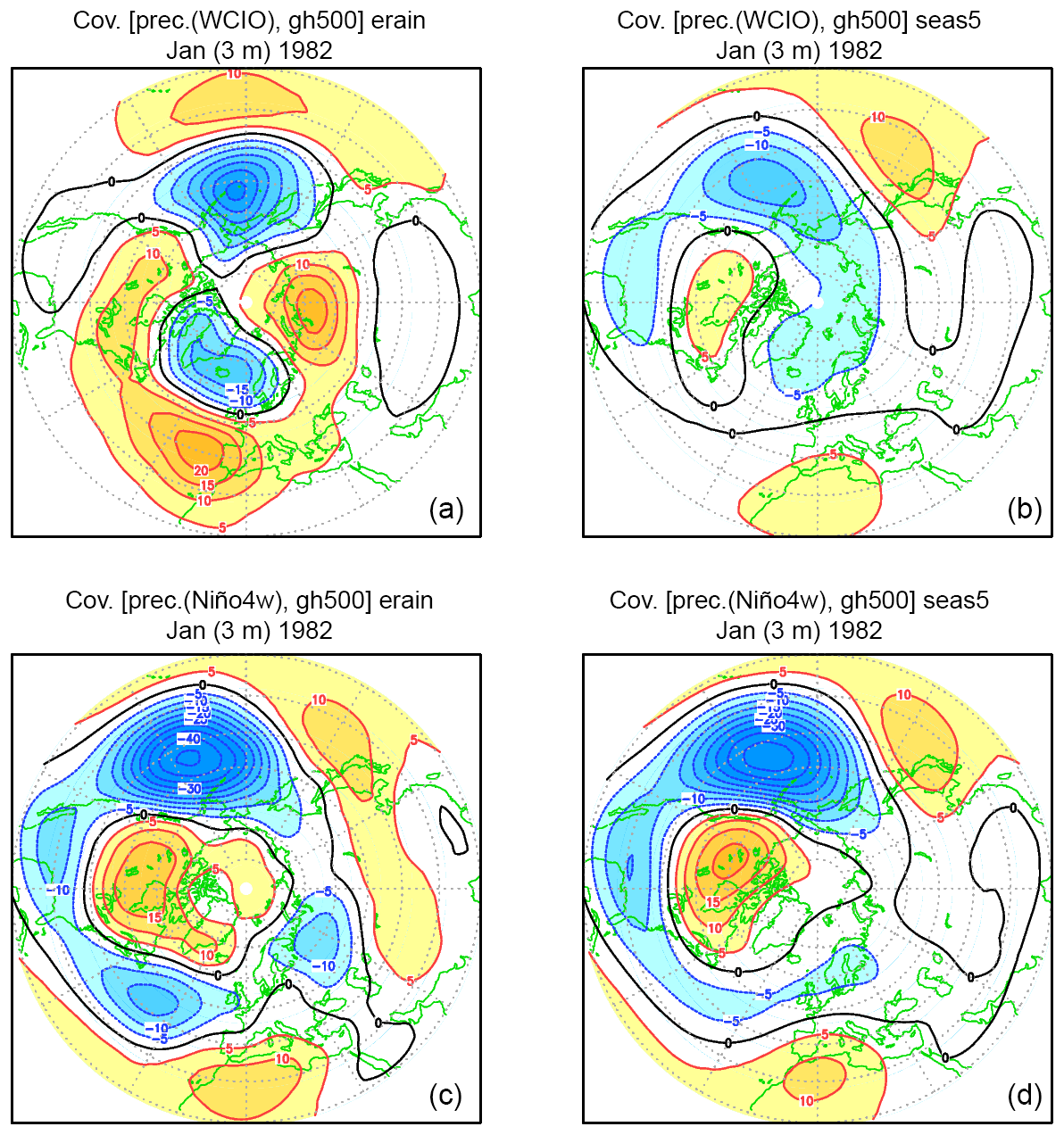
Figure 14Covariances between normalised DJF rainfall anomalies in the western and central Indian Ocean (WCIO, a, b) and Niño 4w (c, d) regions, and 500 hPa height anomalies over the northern extratropics for 1981 to 2016. (a, c) From GPCP v2.3 rainfall and ERA-Interim geopotential height data; (b, d) from SEAS5 re-forecasts. SEAS4 results are shown in Fig. 6 in MVF15.
The reasons for both the improvements and deterioration of extratropical teleconnections in SEAS5 are still being investigated. The improved simulation of the ENSO response is consistent with the general improvements in the representation of ENSO reported in previous sections of this paper. The deterioration of the WCIO–North Atlantic connection is also evident in multi-decadal coupled simulations run for the PRIMAVERA project (Roberts et al., 2018) and performed with the same IFS and NEMO versions used in SEAS5. Simulations analogous to SEAS5 and to the multi-decadal simulations which use prescribed, observed SST show a much better agreement with observations (Franco Molteni, Christopher D. Roberts and Retish Senan, personal communication, 2018). Since links between Indian Ocean rainfall and the NAO are also evident on the sub-seasonal timescale (Cassou, 2008; Lin et al., 2009), future analysis of SEAS5 performance in reproducing tropical intra-seasonal variability (such as the Madden–Julian Oscillation) and the associated ocean–atmosphere feedbacks may shed light on the causes of deficiencies detected on the seasonal timescale.
4.3 Arctic
SEAS5 is the first seasonal forecast system at ECMWF to contain an interactive sea-ice model. SEAS4 prescribed sea ice in re-forecasts and forecasts using an empirical scheme that sampled ERA-Interim data from the five previous years. Consequently, SEAS4 was able to capture the long-term trends in sea-ice evolution, but not the inter-annual variability of sea ice. Sea-ice forecasts are relevant for industries such as shipping and fishing. Sea ice also has locally strong impacts on the forecasts of near-surface parameters and may affect mid-latitude weather through teleconnections. The LIM2 model enables SEAS5 to forecast inter-annual variability in sea-ice concentration. However, the introduction of a fully prognostic sea-ice model introduces biases in the hindcast set. Seasonal Arctic sea-ice biases for SEAS5 are shown in Fig. 15, relative to the OSI SAF global sea-ice concentration climate data record (OSI-450, see Sect. 3.2 for details). The most noticeable biases are excess sea ice in the summer, due to not enough seasonal melting of the ice in SEAS5, and a lack of sea ice in the autumn, due to slow re-freezing of the ice. In spring, summer and winter there is excess ice in the Greenland Sea, along the Odden ice tongue. This bias is caused by ice that remains in later decades in SEAS5, which is rarely present after the 1990s in reanalysis.
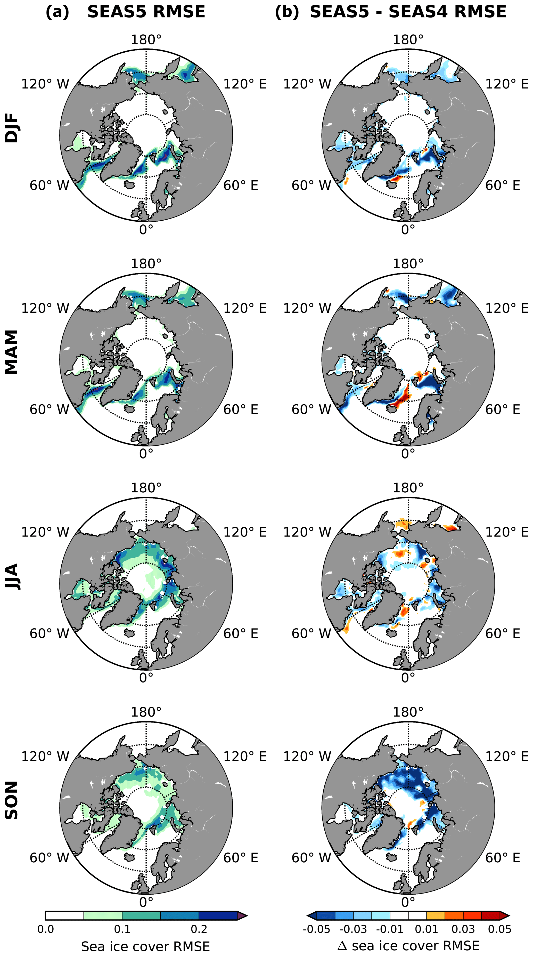
Figure 16SEAS5 bias-corrected seasonal Arctic sea-ice concentration RMSE maps (a) relative to OSI-450, and the difference compared to SEAS4 (b) at 1 month lead time. Twenty-five ensemble members are used from each forecast system. Due to gaps in the satellite record, a small number of seasons had to be excluded from this analysis (see Sect. 3.2 for details).
Despite introducing these biases, including the interactive sea-ice model improves the skill in predicting the inter-annual variability in sea ice. This is illustrated in the sea-ice concentration RMSE maps shown in Fig. 16. As with other variables, sea-ice concentration is bias corrected before calculation of RMSE, but as sea-ice concentration is a value that varies between 0 and 1, grid points were not bias corrected to values greater than 1 or less than 0. The RMSE in SEAS5 is typically 10 %–25 %, which is an improvement over SEAS4 of 1 %–3 % in many locations and up to 5 % in some places. The largest improvements are seen in autumn, probably because autumn is the season most affected by inter-annual variability. There are regions where the RMSE increases, such as in the Bering Straight and Okhotsk Sea in summer and in the location of the Odden ice tongue bias in spring; but overall, LIM2 is having a positive effect on forecasts of sea-ice anomalies.
4.4 Stratosphere and QBO
Dynamical processes in the stratosphere are increasingly seen as a possible source of seasonal predictability. Teleconnections from the tropical oceans to the mid-latitudes may be mediated by the stratosphere (Bell et al., 2009; Ineson and Scaife, 2009), placing importance on correctly representing the mean stratosphere climate (Maycock et al., 2011). Additionally, the quasi-biennial oscillation of the tropical stratosphere (QBO; Reed et al., 1961) potentially provides one of the few purely atmospheric sources of predictability on the seasonal timescale (e.g. Ebdon, 1975; Folland et al., 2012).

Figure 17Zonally averaged profiles of ERA-Interim DJF zonal temperature (a) and wind (b), as well as biases in SEAS4 (c, d) and SEAS5 (e, f) at 1 month forecast lead.
Figure 17 shows DJF zonal wind and temperature profiles in the troposphere and stratosphere for SEAS4 and SEAS5, extending the profiles shown in Fig. 8 to 1 hPa. As discussed in Sect. 4.2, SEAS4 had a pervasive 0.5 to 2.0 ∘C cold bias to a height of about 20 hPa, with a warm bias above it. The cold bias disappeared in the troposphere in SEAS5, but increased to as much as 5 ∘C in the lower stratosphere, just above the tropopause. At about 10 hPa in the tropics, this cold bias transitions to a warm bias in the upper stratosphere. These changes correspond to a steepening of the temperature gradient from the lower to upper stratosphere. The tropopause cold temperature bias in SEAS5 is accompanied by errors in the mid-latitude jets at the tropopause level (see Sect. 4.2) and excess equatorial westerly wind biases are present above 40 hPa. These excess winds were also present in SEAS4, but have worsened in SEAS5. The boreal winter-time polar vortex weakens in SEAS5, resulting in an easterly bias throughout the depth of the stratosphere. Corresponding bias changes are seen in JJA: both in the winter (southern) hemisphere and the tropics.
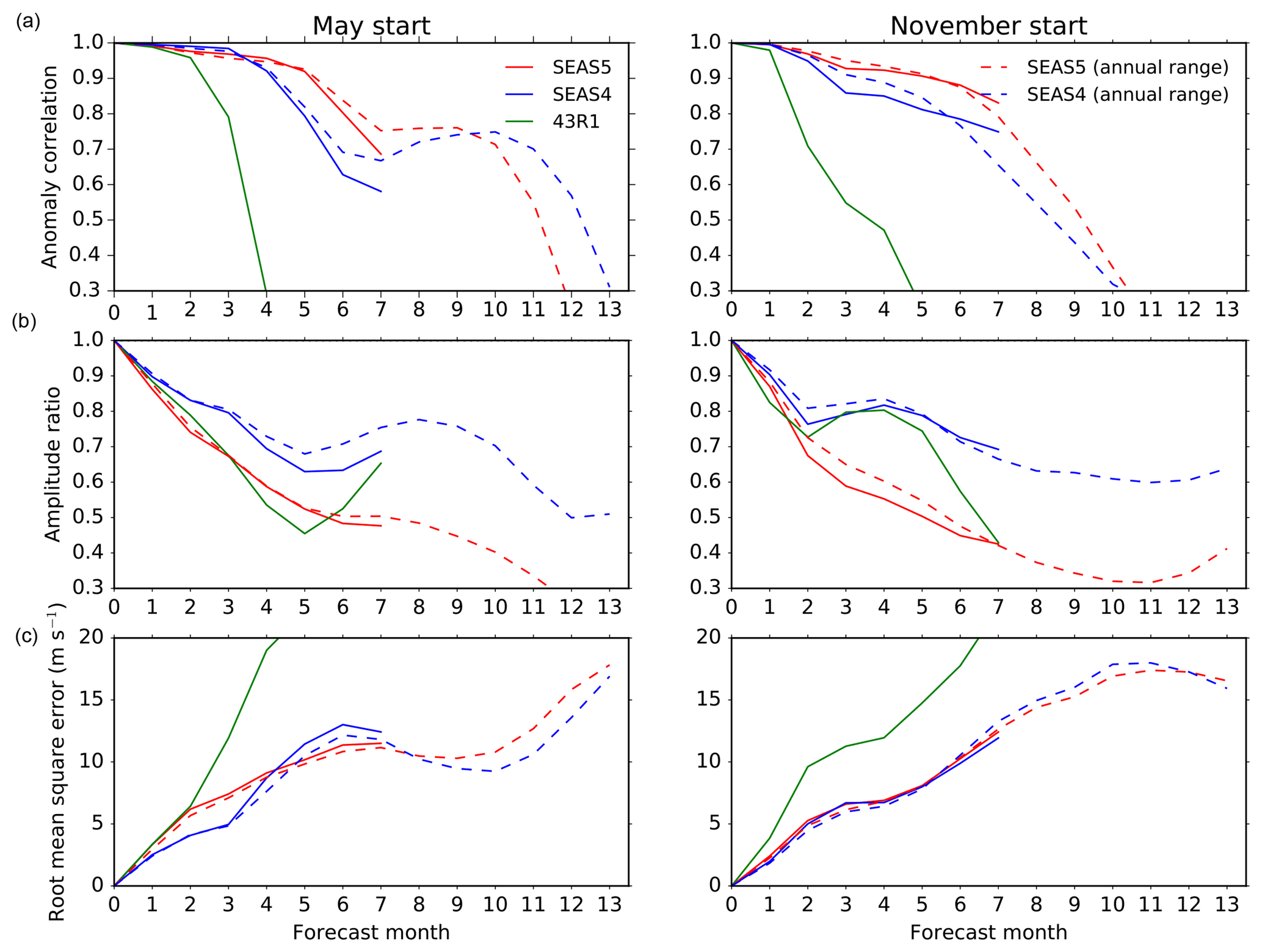
Figure 18Metrics summarising the phase and amplitude of a QBO index at 30 hPa in SEAS4 (blue), SEAS5 (red) and IFS cycle 43r1 with default settings (green) relative to ERA-Interim reanalysis for forecasts initialised in May and November. (a) Anomaly correlation, (b) ratio of the standard deviation of the system to the standard deviation of ERA-Interim reanalysis and (c) RMSE. To compare SEAS4 and SEAS5 fairly with the data available for the default 43r1 cycle, the solid lines use only 5 ensemble members with initialisation dates from 1993 to 2015. The dashed lines compare SEAS4 and SEAS5 for the entire 13 month duration of the annual-range forecasts from 1981 to 2016, using the 15 ensemble members.
As mentioned in Sect. 2.2, the tropical non-orographic gravity wave drag was reduced from its default value in IFS cycle 43r1 in order to improve the representation of the QBO in SEAS5. To illustrate the motivation and result of this change, we compare in Fig. 18 the amplitude and phase of a QBO index as a function of lead time for SEAS4, the default cycle 43r1 IFS, and SEAS5 as the solid lines. We also show the annual-range forecast for SEAS4 and SEAS5 as the dashed lines. To compare SEAS4 and SEAS5 fairly with the smaller dataset available for the default IFS cycle 43r1, we use only five ensemble members with initialisation dates from 1993 to 2015, while the annual-range forecasts contain 15 ensemble members with initialisation dates from 1981 to 2016. This illustrates that the number of ensemble members and years has some effect on statistics of QBO skill, as shown by the differences between the dashed and solid lines. We use the monthly zonal wind averaged from 5∘ N to 5∘ S at 30 hPa as a QBO index.
The anomaly correlation of the default IFS cycle 43r1 decreases sharply after month 2 in forecasts initialised in both May and November. For the November initialisation the correlation is comparable to, or just exceeding, a persistence forecast (not shown), while for the May initialisation the first few months exceed persistence. In contrast, SEAS5 improves on SEAS4, and has an anomaly correlation exceeding 0.7 throughout the long-range forecast. The QBO amplitude is lower in SEAS4 than in ERA-Interim reanalysis, and this reduces even more in SEAS5. Reducing the tropical non-orographic gravity wave drag does not improve the amplitude of the QBO; in the forecast initialised in November it even degrades the amplitude further. However, the combination of the improvement in anomaly correlation and the degradation in amplitude results in a comparable QBO RMSE in SEAS4 and SEAS5, whereas the default IFS cycle 43r1 has a much larger RMSE. Reducing the tropical non-orographic gravity wave drag also reduces the equatorial zonal wind bias around 10 hPa (not shown), though a large bias remains. However, lower in the stratosphere the QBO deteriorates in both phase and amplitude compared to SEAS4 (not shown), despite the reduction in the tropical non-orographic gravity wave drag.
As lead time increases, the QBO amplitude in SEAS5 decreases and worsens relative to SEAS4. The RMSE in the annual-range forecast is large in both systems, though it shows more skill than a persistence forecast. Differences between the SEAS4 and SEAS5 anomaly correlations of the annual-range forecast depend on season and lead time. Differences between the two systems' RMSE in the annual-range forecasts are small compared to the RMSE of either system.
Although predicting the QBO phase is potentially important for improving the seasonal forecast skill, the realisation of this skill relies on the teleconnections between the QBO and the extratropics, which are generally not very well represented in seasonal systems (Scaife et al., 2014). Future work will evaluate this teleconnection in SEAS5.
In the previous section we discussed the performance of SEAS5 from the perspective of model development and predictability. In this section, we present verification metrics corresponding to the SEAS5 operational charts and focus on the skill of variables more relevant for users: 2 m temperature and precipitation. Here, we discuss DJF and JJA at 1 month lead time. A more comprehensive set of seasonal forecast skill measures including all seasons, lead times and additional atmospheric variables is available on ECMWF's website.6
We first use maps of the temporal anomaly correlation of the forecast ensemble mean anomalies with the observed anomalies to show the geographical distribution of skill over the globe. The use of deterministic skill measures, such as the anomaly correlation of the ensemble mean, is common practise despite the probabilistic nature of the seasonal predictions. To add a probabilistic measure of skill we then discuss differences in continuous ranked probability skill score (CRPSS) between SEAS4 and SEAS5. Finally, we discuss SEAS5 2 m temperature reliability over the tropics and Europe.
As discussed in Sect. 3, the re-forecast set we evaluate here has 25 members, while operational forecasts have 51 members. Consequently, the skill estimates based on the re-forecasts are a systematic underestimate of the expected skill of the operational ensemble, although a real-time system also carries a slightly higher risk of issues such as unexpected changes in observing systems or unpredicted changes in climate system behaviour.
5.1 Anomaly correlation
Figure 19(a, b) Anomaly correlation map of the ensemble-mean SEAS5 mean 2 m temperature forecast for DJF (a, c) and JJA (b, d) at 1 month forecast lead. 2 m temperature is verified with ERA-Interim data. Locations with correlation values different from zero at the 5 % significance level are highlighted by dots. (c, d) Difference between SEAS5 and SEAS4 anomaly correlation, with 25 ensemble members used in each. Locations where the correlation values are different at a 5 % significance level are highlighted by dots.
In Fig. 19 the geographical distribution of 2 m temperature skill at 1 month lead time is represented by the local correlation between ensemble-mean of the re-forecasts and ERA-Interim. High skill for near-surface temperature is evident over the tropics, particularly over the tropical oceans where skill reaches a maximum in the central and east Pacific. A number of extra-tropical regions, depending on the season, also show useful skill. In DJF, SEAS5 shows some level of skill across northern and central Europe, with areas of significance over Scandinavia. In JJA, we see significant skill over southeastern Europe and the Mediterranean. Some of this skill is associated with the model's ability to represent the longer-term trends (decadal variability and climate change) as well as its ability to correctly forecast inter-annual variability.
Forecast skill is low in places over continental North America and Eurasia, which is common in seasonal forecast systems (Molteni et al., 2011; Kim et al., 2012; Maclachlan et al., 2015), and is also evident in MSLP and 500 hPa geopotential skill (not shown). There is a region over the northwest Atlantic by the Grand Banks of Newfoundland with negative correlation values in DJF. As discussed in Sect. 4.2, SEAS5 poorly captures the observed decadal variability in the North Atlantic subpolar gyre, which decreases skill in this region. There are also skill minima over other ocean boundary currents, though little is known about the potential predictability in these regions.
Figure 19 also shows the difference in 2 m temperature skill between SEAS5 and SEAS4. In the tropics, improvements in DJF are found in the tropical and subtropical eastern Pacific reaching the west coast of America, likely associated with the improvements in ENSO bias and variability discussed in Sect. 4.1. A degradation is seen in the EEIO in JJA, due to the errors in EEIO variability also discussed in Sect. 4.1. In JJA, significant improvements in skill are seen over equatorial Africa and tropical North America and tropical South America.
In the extratropics, some improvement in JJA skill is found over Greenland and eastern Siberia. Figure 19 also shows the decrease in skill over the northwest Atlantic (Sect. 4.2). There is no evidence of locally significant skill improvement over Europe in either season. There is an overall improvement in 2 m temperature predictions north of 60∘ N and south of 60∘ S in both seasons, including a substantial enhancement of JJA skill found in the Southern Hemisphere. This is likely to be related to the improved predication of sea-ice concentration generated by the addition of LIM2. At longer time ranges (month 5 to 7, not shown) SEAS5 exhibits enhanced skill over large areas of the tropical oceans (0–20∘ N).
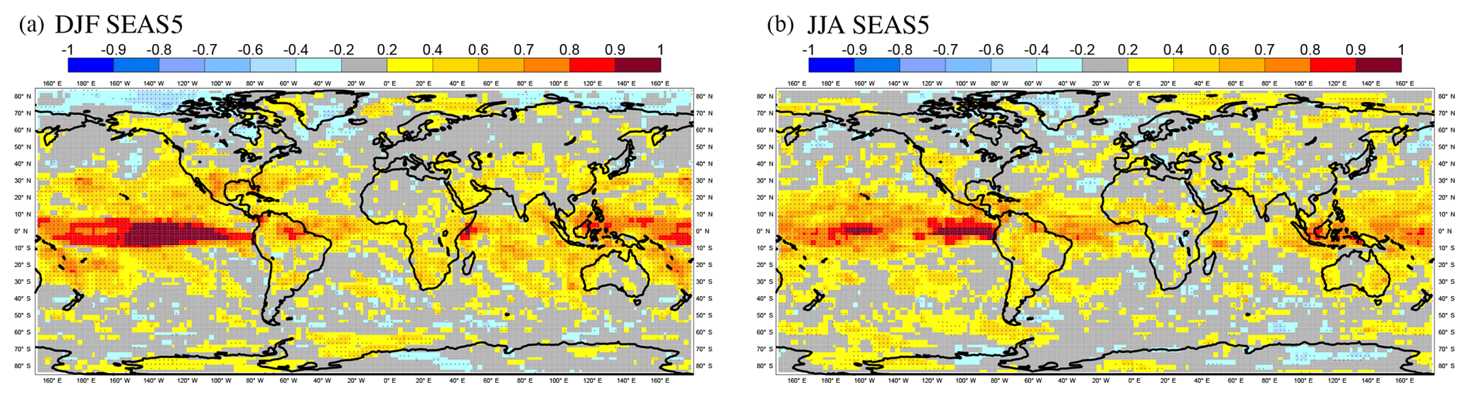
Figure 20Anomaly correlation maps of the SEAS5 ensemble-mean precipitation forecast for DJF (a) and JJA (b) at 1 month forecast lead. Precipitation is verified with GPCP v2.2 data from 1981 to 2014. Locations with correlation values different from zero at the 5 % significance level are highlighted by dots.
In Fig. 20, we show the anomaly correlation maps of SEAS5 precipitation compared to GPCP2.2 (1981–2014). Precipitation skill is much noisier and significantly lower than the skill for near-surface temperature. Over the tropical oceans the signal looks more coherent, while seasonal prediction for rainfall over land generally has lower skill, even in the tropics. “Local” (i.e. grid-point) seasonal rainfall predictions often have limited skill, but spatially averaged values over many tropical regions have significant predictability and play a crucial role for extratropical predictability (Molteni et al., 2015; Scaife et al., 2017, 2018). Differences in rainfall anomaly correlation between SEAS4 and SEAS5 are noisy, so we discuss differences in precipitation skill using CRPSS in the next section.
5.2 CRPSS
It is common to use CRPSS, the skill score version of the continuous ranked probability score (CRPS; Hersbach, 2000; Matheson and Winkler, 1976; Wilks, 2011), to evaluate the benefit of a forecasting system. The CRPS is the integral of the Brier score over all possible threshold values for a given variable. For a deterministic forecast the CRPS reduces to the mean absolute error. The CRPSS then gives an indication of the added value of a forecasting system over simply forecasting climatology, a value of 1 indicating perfect forecasts, 0 showing no improvement over climatology and negative values indicating a failing forecasting system. In Fig. 21, we use maps of 2 m temperature SEAS5 CRPSS relative to ERA-Interim and CRPSS differences between SEAS4 and SEAS5 to highlight the changes in probabilistic skill between SEAS5 and SEAS4 (see Sect. 3.1 for a description of how the CRPSS is calculated).
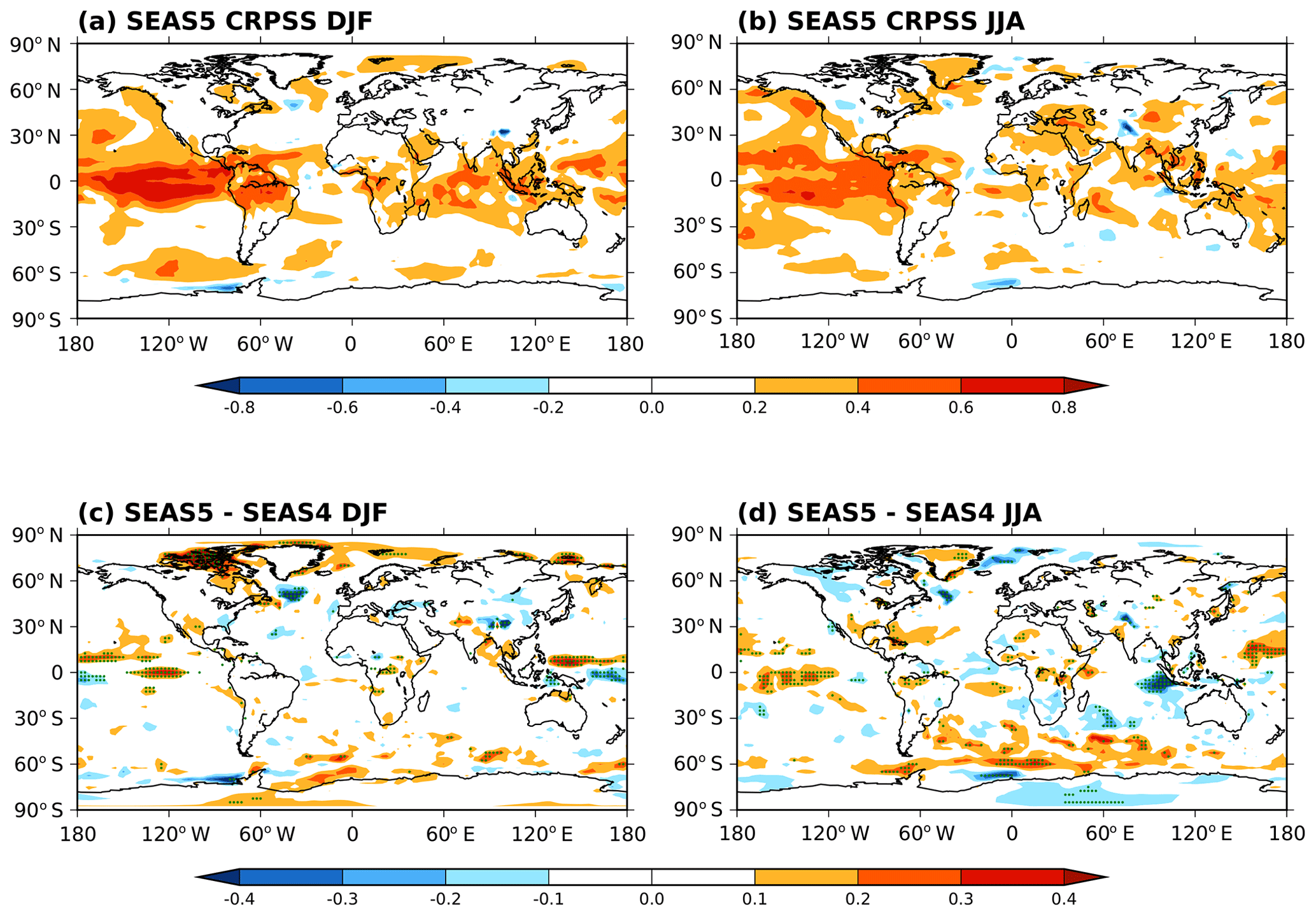
Figure 21(a, b) CRPSS maps of 2 m temperature for SEAS5 with reference to ERA-Interim climatology in (a) DJF and (b) JJA. (c, d) The change in 2 m temperature CRPSS score between SEAS5 and SEAS4 in (c) DJF and (d) JJA. Green stippling is plotted at p<0.05.
SEAS5 CRPSS relative to ERA-Interim demonstrates that SEAS5 generally provides improved skill in the tropics compared to ERA-Interim climatology. Outside the tropics, there are a few, seasonally dependent, regions where SEAS5 skill exceeds climatology. Regions with negative scores are small, but often correspond to known deficiencies in the system including in the North Atlantic in DJF and the EEIO in JJA.
The changes in CRPSS broadly agree with the changes in anomaly correlation seen in Fig. 19. The tropical Pacific shows improvement across the basin in JJA. In DJF, this improvement extends from 120∘ E to 120∘ W, but is confined to the north of the Equator, while to the south there is some deterioration. The improvement seen in eastern equatorial Africa in the anomaly correlation maps is also present in CRPSS. The deterioration in the North Atlantic and EEIO is also evident. Over the Himalayas little decrease in skill is seen in the anomaly correlation maps, but a clear decrease is seen in CRPSS. This may indicate a change in the spread in SEAS5, but further analysis is needed to understand this feature. Areas of significant improvement and deterioration are evident in both hemispheres around the edges of the sea ice, though not as widespread as in anomaly correlation.

Figure 22(a, b) CRPSS maps of precipitation for SEAS5 with reference to GPCP climatology (1981–2014) in (a) DJF and (b) JJA. (c, d) The change in precipitation CRPSS score between SEAS5 and SEAS4 in (c) DJF and (d) JJA. Green stippling is plotted at p<0.05.

Figure 23DJF 2 m temperature reliability diagrams for SEAS5, computed including all grid points for the tropics (a, 20∘ N to 20∘ S) and a European region (b, 35 to 75∘ N, 12.5∘ W to 42.5∘ E) over the whole re-forecast period using 25 ensemble members. Verification data are ERA-Interim. Reliability diagrams are computed for 3-month average forecast anomalies in the upper third of the model climate distribution. Grey vertical lines indicate the 95 % confidence intervals.
CRPSS maps of precipitation are shown in Fig. 22. SEAS5 has a narrow equatorial band of skill relative to GPCP climatology, which extends from the Maritime Continent across the Pacific Ocean and South America to the western Atlantic Ocean. CRPSS values are higher in DJF than in JJA, due to the influence of ENSO. In JJA, there are two larger areas where the GPCP climatology is more skillful than SEAS5: in the eastern equatorial Atlantic and south of the Equator in the eastern Pacific (see Fig. 22a and b). Differences from SEAS4 are noisy, but more coherent patterns are present in a few locations. In JJA, the precipitation skill is improved substantially over the eastern Maritime Continent relative to SEAS4 (Fig. 22d). This improvement continues into the later months of the forecast (forecast months 5 to 7) to show a large increase in skill over the tropical west Pacific in the autumn (not shown). There is a decrease in skill in the eastern equatorial Pacific in both seasons. The CRPSS differences over the tropical Atlantic (Fig. 22c and d) indicate a large SEAS5 improvement in both seasons. Skill scores such as the CRPSS measure the accuracy of a forecast with respect to the accuracy of a reference forecast which, in our case, is the observed climatology. The result is that CRPSS emphasises SEAS5 improvements in regions where a GPCP climatological forecast has higher skill than both systems, such as the tropical Atlantic.
5.3 Reliability
Reliability measures the ability of a forecast system to represent the observed frequency of events. Reliability is an important consideration for the usefulness of probabilistic predictions, as a user might be able to make use of a forecasting system with limited skill if the system is statistically reliable. Reliability is typically illustrated using reliability diagrams (see Sect. 3.1.5). In a perfectly reliable system, the forecast probability will equal the frequency of occurrence and points will lie along a straight diagonal line. Figure 23 shows reliability diagrams for warm 2 m temperature anomalies in DJF. Forecasts in the tropics (20∘ N to 20∘ S) show a small but systematic discrepancy between the forecast probabilities and observed frequencies where forecast probabilities for the event are further from climatology than is observed. This is a common property of seasonal forecast systems, often referred to as “overconfidence” (Weisheimer and Palmer, 2014). Over Europe and its surrounding seas (35 to 75∘ N, 12.5∘ W to 42.5∘ E), the forecast also tends to be overconfident, though reliability over land points is lower than reliability over sea points in this region. Comparisons with SEAS4 reliability indicate only small changes in reliability between SEAS4 and SEAS5 (not shown).
ECMWF's fifth seasonal forecast system, SEAS5, became operational in November 2017, replacing its predecessor SEAS4. SEAS5 features upgraded versions and increased resolution of the atmosphere and ocean models as well as adding the interactive sea-ice model LIM2. It also represents a step towards a seamless system, with very few differences from the cycle 43r1 extended range (monthly) forecast system.
SEAS5 improves on SEAS4 in a number of ways. There is clear improvement in equatorial Pacific SST bias and in the cold bias present throughout the troposphere in SEAS4. SEAS5 skill in ENSO prediction increases, especially in the western-central Pacific and in the annual-range forecasts, improving on already high skill in SEAS4. In spite of this noticeable skill improvement, ENSO forecasts remain overconfident (under-dispersive). The interactive sea-ice model gives SEAS5 the ability to forecast sea-ice concentration. This leads to improved predictions of Arctic sea ice and improved 2 m temperature prediction skill around the sea-ice edge.
Other aspects of SEAS5 are degraded compared to SEAS4. The variability in the eastern equatorial Indian Ocean is very overactive in SEAS5, posing a problem for teleconnections originating there. Skill has decreased in the northwest Atlantic where SEAS5 fails to capture decadal variability; an error which was not present in SEAS4. Temperature biases in the lower stratosphere and jets at the tropopause level are also degraded in SEAS5 relative to SEAS4, which could be inhibiting teleconnections and preventing increased tropical skill from generating increased extratropical skill. These issues are actively being investigated in order to improve future seasonal forecast systems.
Overall, SEAS5 is another step in the development of seasonal forecast systems at ECMWF, with advances generating higher levels of skill where expected (e.g. interactive sea ice), while some known deficiencies remain and others appear. SEAS5 continues to be a state-of-the-art seasonal forecast system, with a particular strength in ENSO prediction. SEAS5 forecasts and re-forecasts are contributed to the Copernicus Climate Change Service's (C3S) multi-system seasonal forecast and are publicly available from the C3S climate data store with data from other state-of-the-art seasonal forecast systems. This creates opportunities for a wide range of research on seasonal forecasting and predictability and could be a catalyst for future seasonal forecast development.
The model configurations described here are based on the ECMWF Integrated Forecast System (IFS) and the NEMO/LIM ocean–sea-ice model. The IFS source code is available subject to a license agreement with ECMWF. ECMWF member-state weather services and their approved partners will be granted access. The IFS code without modules for data assimilation is also available for educational and academic purposes as part of the OpenIFS project (https://software.ecmwf.int/wiki/display/OIFS/OpenIFS+Home, last access: 12 September 2018). The NEMO/LIM source code is available under a CeCILL free software license (https://www.nemo-ocean.eu/, last access: 12 September 2018).
The re-forecasts from SEAS5 are publicly available from ECMWF's Copernicus Climate Change Service (C3S), through its climate data store (https://doi.org/10.21957/p3c285, Raoult et al., 2017). Instructions on how to access these data are available from the C3S user support. SEAS4 is not a public dataset; to access SEAS4 data please contact the authors with a specific request.
SJJ, TNS, LF, MAB, FM, LM, ST, DD and AW contributed to the configuration of SEAS5 and the assessment presented in this article. MAB, GB, SK, KM and HZ contributed to the development of components of the coupled forecast model used in SEAS5. BMS contributed to the development and assessment of the ozone model employed in SEAS5.
The authors have no competing interests.
We would like to acknowledge all ECMWF staff who have actively contributed to the development of the IFS model and the successful implementation of SEAS5. The authors specifically acknowledge Richard Forbes, who contributed a written description of the IFS model differences between cycle 36r4 and cycle 43r1 to this article. We would also like to acknowledge two anonymous reviewers, whose feedback improved the article.
This study has been partially funded by the Copernicus Climate Change Service. ECMWF
implements this service and the Copernicus Atmosphere Monitoring Service on behalf of the
European Commission.
Edited by: Sophie Valcke
Reviewed by: two anonymous referees
Adler, R. F., Huffman, G. J., Chang, A., Ferraro, R., Xie, P.-P., Janowiak, J., Rudolf, B., Schneider, U., Curtis, S., Bolvin, D., Gruber, A., Susskind, J., Arkin, P., and Nelkin, E.: The Version-2 Global Precipitation Climatology Project (GPCP) Monthly Precipitation Analysis (1979–Present), J. Hydrometeorol., 4, 1147–1167, https://doi.org/10.1175/1525-7541(2003)004<1147:TVGPCP>2.0.CO;2, 2003. a
Ahlgrimm, M. and Forbes, R.: Improving the representation of low clouds and drizzle in the ECMWF model based on ARM observations from the Azores, Mon. Weather Rev., 142, 668–685, 2014. a
Balmaseda, M. A., Mogensen, K., and Weaver, A. T.: Evaluation of the ECMWF ocean reanalysis system ORAS4, Q. J. Roy. Meteor. Soc., 139, 1132–1161, https://doi.org/10.1002/qj.2063, 2013. a, b
Balsamo, G., Beljaars, A., Scipal, K., Viterbo, P., van den Hurk, B., Hirschi, M., and Betts, A. K.: A revised hydrology for the ECMWF model: Verification from field site to terrestrial water storage and impact in the Integrated Forecast System, J. Hydrometeorol., 10, 623–643, 2009. a, b
Balsamo, G., Salgado, R., Dutra, E., Boussetta, S., Stockdale, T., and Potes, M.: On the contribution of lakes in predicting near-surface temperature in a global weather forecasting model, Tellus A, 64, 15829, https://doi.org/10.3402/tellusa.v64i0.15829, 2012. a
Balsamo, G., Albergel, C., Beljaars, A., Boussetta, S., Brun, E., Cloke, H., Dee, D., Dutra, E., Muñoz-Sabater, J., Pappenberger, F., de Rosnay, P., Stockdale, T., and Vitart, F.: ERA-Interim/Land: a global land surface reanalysis data set, Hydrol. Earth Syst. Sci., 19, 389–407, https://doi.org/10.5194/hess-19-389-2015, 2015. a
Barnston, A. G., Tippett, M. K., L'Heureux, M. L., Li, S., and Dewitt, D. G.: Skill of real-time seasonal ENSO model predictions during 2002–11: Is our capability increasing?, B. Am. Meteorol. Soc., 93, 631–651, https://doi.org/10.1175/BAMS-D-11-00111.1, 2012. a
Bechtold, P., Köhler, M., Jung, T., Doblas-Reyes, F., Leutbecher, M., Rodwell, M. J., Vitart, F., and Balsamo, G.: Advances in simulating atmospheric variability with the ECMWF model: From synoptic to decadal time-scales, Q. J. Roy. Meteor. Soc., 134, 1337–1351, 2008. a
Bechtold, P., Semane, N., Lopez, P., Chaboureau, J.-P., Beljaars, A., and Bormann, N.: Representing Equilibrium and Nonequilibrium Convection in Large-Scale Models, J. Atmos. Sci., 71, 734–753, https://doi.org/10.1175/JAS-D-13-0163.1, 2014. a, b
Beljaars, A., Brown, A. R., and Wood, N.: A new parametrization of turbulent orographic form drag, Q. J. Roy. Meteor. Soc., 130, 1327–1347, 2004. a
Bell, C. J., Gray, L. J., Charlton-Perez, A. J., Joshi, M. M., and Scaife, A. A.: Stratospheric communication of El Niño teleconnections to European winter, J. Climate, 22, 4083–4096, https://doi.org/10.1175/2009JCLI2717.1, 2009. a
Boussetta, S., Balsamo, G., Beljaars, A., Kral, T., and Jarlan, L.: Impact of a satellite-derived leaf area index monthly climatology in a global numerical weather prediction model, Int. J. Remote Sens., 34, 3520–3542, https://doi.org/10.1080/01431161.2012.716543, 2013. a
Breivik, Ø., Mogensen, K., Bidlot, J.-R., Balmaseda, A., and Janssen, P. A. E. M.: Surface wave effects in the NEMO ocean model: Forced and coupled experiments, J. Geophys. Res.-Oceans, 120, 2973–2992, https://doi.org/10.1002/2014JC010565, 2015. a
Brown, A., Milton, S., Cullen, M., Golding, B., Mitchell, J., and Shelly, A.: Unified modeling and prediction of weather and climate: A 25-year journey, B. Am. Meteorol. Soc., 93, 1865–1877, https://doi.org/10.1175/BAMS-D-12-00018.1, 2012. a
Buckley, M. W. and Marshall, J.: Observations, inferences, and mechanisms of the Atlantic Meridional Overturning Circulation: A review, Rev. Geophys., 54, 5–63, https://doi.org/10.1002/2015RG000493, 2016. a
Buizza, R., Hollingsworth, A., Lalaurette, F., and Ghelli, A.: Probabilistic Predictions of Precipitation Using the ECMWF Ensemble Prediction System, Weather Forecast., 14, 168–189, https://doi.org/10.1175/1520-0434(2000)015<0365:COPPOP>2.0.CO;2, 1999. a
Cariolle, D. and Déqué, M.: Southern hemisphere medium-scale waves and total ozone disturbances in a spectral general circulation model, J. Geophys. Res.-Atmos., 91, 10825–10846, 1986. a
Cariolle, D. and Teyssèdre, H.: A revised linear ozone photochemistry parameterization for use in transport and general circulation models: multi-annual simulations, Atmos. Chem. Phys., 7, 2183-2196, https://doi.org/10.5194/acp-7-2183-2007, 2007. a
Cassou, C.: Intraseasonal interaction between the Madden Julian Oscillation and the North Atlantic Oscillation, Nature, 455, 523–527, 2008. a
Charney, J. and Shukla, J.: Predictability of monsoons, in: Monsoon Dynamics, edited by: Lighthill, J. and Pearce, R. P., chap. 6, 99–110, Cambridge University Press, Cambridge, https://doi.org/10.1017/CBO9780511897580.009, 1981. a
Chassignet, E. P. and Marshall, D. P.: Gulf Stream Separation in Numerical Ocean Models, in: Ocean Modeling in an Eddying Regime, edited by: Hecht, M. W. and Hasumi, H., Geophysical Monograph Series, 177, 39–61, https://doi.org/10.1029/177GM05, 2008. a
Craig, P. D. and Banner, M. L.: Modeling Wave-Enhanced Turbulence in the Ocean Surface Layer, 24, 2546–2559, https://doi.org/10.1175/1520-0485(1994)024<2546:MWETIT>2.0.CO;2, 1994. a
de Rosnay, P., Balsamo, G., Albergel, C., Muñoz-Sabater, J., and Isaksen, L.: Initialisation of land surface variables for Numerical Weather Prediction, Surv. Geophys., 35, 607–621, https://doi.org/10.1007/s10712-012-9207-x, 2014. a
Dee, D. P., Uppala, S. M., Simmons, A. J., Berrisford, P., Poli, P., Kobayashi, S., Andrae, U., Balmaseda, M. A., Balsamo, G., Bauer, P., Bechtold, P., Beljaars, A. C. M., Berg, L. V. D., Bidlot, J., Bormann, N., Delsol, C., Dragani, R., Fuentes, M., Geer, A. J., Dee, D. P., van de Berg, L., Bidlot, J., Bormann, N., Delsol, C., Dragani, R., Fuentes, M., Geer, A. J., Haimberger, L., Healy, S. B., Hersbach, H., Hólm, E. V., Isaksen, L., Kållberg, P., Köhler, M., Matricardi, M., Mcnally, A. P., Monge-Sanz, B. M., Morcrette, J. J., Park, B. K., Peubey, C., de Rosnay, P., Tavolato, C., Thépaut, J. N., and Vitart, F.: The ERA-Interim reanalysis: configuration and performance of the data assimilation system, Q. J. Roy. Meteor. Soc., 137, 553–597, https://doi.org/10.1002/qj.828, 2011. a, b, c
Deser, C., Alexander, M. A., Xie, S.-P., and Phillips, A. S.: Sea Surface Temperature Variability: Patterns and Mechanisms, Ann. Rev. Mar. Sci., 2, 115–143, https://doi.org/10.1146/annurev-marine-120408-151453, 2010. a
Donlon, C. J., Martin, M., Stark, J., Roberts-Jones, J., Fiedler, E., and Wimmer, W.: The Operational Sea Surface Temperature and Sea Ice Analysis (OSTIA) system, Remote Sens. Environ., 116, 140–158, https://doi.org/10.1016/j.rse.2010.10.017, 2012. a
Dunstone, N., Smith, D., Scaife, A., Hermanson, L., Eade, R., Robinson, N., Andrews, M., and Knight, J.: Skilful predictions of the winter North Atlantic Oscillation one year ahead, Nat. Geosci., 9, 809–814, https://doi.org/10.1038/ngeo2824, 2016. a
Dutra, E., Balsamo, G., Viterbo, P., Miranda, P. M. A., Beljaars, A., Schär, C., and Elder, K.: An improved snow scheme for the ECMWF land surface model: Description and offline validation, J. Hydrometeorol., 11, 899–916, 2010a. a, b
Dutra, E., Stepanenko, V. M., Balsamo, G., Viterbo, P., Miranda, P., Mironov, D., and Schär, C.: An offline study of the impact of lakes in the performance of the ECMWF surface scheme, Boreal Environ. Res., 15, 100–112, 2010b. a
Ebdon, R. A.: The quasibiennial oscillation and its association with tropospheric circulation patterns, Meteorol. Mag., 104, 282–297, 1975. a
Fichefet, T. and Maqueda, M. A.: Sensitivity of a global sea ice model to the treatment of ice thermodynamics and dynamics, J. Geophys. Res.-Oceans, 102, 12609–12646, https://doi.org/10.1029/97JC00480, 1997. a
Folland, C. K., Scaife, A. A., Lindesay, J., and Stephenson, D. B.: How potentially predictable is northern European winter climate a season ahead?, Int. J. Climatol., 32, 801–818, https://doi.org/10.1002/joc.2314, 2012. a
Forbes, R. M. and Ahlgrimm, M.: On the Representation of High-Latitude Boundary Layer Mixed-Phase Cloud in the ECMWF Global Model, Mon. Weather Rev., 142, 3425–3445, https://doi.org/10.1175/MWR-D-13-00325.1, 2014. a
Forbes, R. M. and Tompkins, A.: An improved representation of cloud and precipitation, ECMWF Newsletter, 129, 13–18, doi:10.21957/nfgulzhe, 2011. a
Forbes, R. M., Tompkins, A. M., and Untch, A.: A new prognastic bulk microphysics scheme for the IFS, ECMWF Technical Memorandam, 649, doi:10.21957/bf6vjvxk, 2011. a
Good, S. A., Martin, M. J., and Rayner, N. A.: EN4: Quality controlled ocean temperature and salinity profiles and monthly objective analyses with uncertainty estimates, J. Geophys. Res.-Oceans, 118, 6704–6716, https://doi.org/10.1002/2013JC009067, 2013. a
Hersbach, H.: Decomposition of the Continuous Ranked Probability Score for Ensemble Prediction Systems, Weather Forecast., 15, 559–570, https://doi.org/10.1175/1520-0434(2000)015<0559:DOTCRP>2.0.CO;2, 2000. a
Hogan, R. J. and Bozzo, A.: Mitigating errors in surface temperature forecasts using approximate radiation updates, J. Adv. Model. Earth Sy., 7, 836–853, 2015. a
Hogan, R. J. and Hirahara, S.: Effect of solar zenith angle specification in models on mean shortwave fluxes and stratospheric temperatures, Geophys. Res. Lett., 43, 482–488, 2016. a
Iacono, M. J., Delamere, J. S., Mlawer, E. J., Shephard, M. W., Clough, S. A., and Collins, W. D.: Radiative forcing by long-lived greenhouse gases: Calculations with the AER radiative transfer models, J. Geophys. Res.-Atmos., 113, D13103, https://doi.org/10.1029/2008JD009944, 2008. a
IFS Documentation CY43R1, ECMWF, available at: https://www.ecmwf.int/en/forecasts/documentation-and-support/changes-ecmwf-model/ifs-documentation (12 September 2018), 2016. a, b, c
Ineson, S. and Scaife, A.: The role of the stratosphere in the European climate response to El Niño, Nat. Geosci., 2, 32–36, 2009. a
Inness, A., Baier, F., Benedetti, A., Bouarar, I., Chabrillat, S., Clark, H., Clerbaux, C., Coheur, P., Engelen, R. J., Errera, Q., Flemming, J., George, M., Granier, C., Hadji-Lazaro, J., Huijnen, V., Hurtmans, D., Jones, L., Kaiser, J. W., Kapsomenakis, J., Lefever, K., Leitão, J., Razinger, M., Richter, A., Schultz, M. G., Simmons, A. J., Suttie, M., Stein, O., Thépaut, J.-N., Thouret, V., Vrekoussis, M., Zerefos, C., and the MACC team: The MACC reanalysis: an 8 yr data set of atmospheric composition, Atmos. Chem. Phys., 13, 4073–4109, https://doi.org/10.5194/acp-13-4073-2013, 2013. a
Janssen, P. A. E. M., Breivik, Ø., Mogensen, K., Vitart, F., Balmaseda, M., Bidlot, J.-r., Keeley, S., Leutbecher, M., Magnusson, L., and Molteni, F.: Air-Sea Interaction and Surface Waves, ECMWF Technical Memorandum, 712, 36 pp., 2013. a
Kim, H. M., Webster, P. J., and Curry, J. A.: Seasonal prediction skill of ECMWF System 4 and NCEP CFSv2 retrospective forecast for the Northern Hemisphere Winter, Clim. Dynam., 39, 2957–2973, https://doi.org/10.1007/s00382-012-1364-6, 2012. a
Köhler, M., Ahlgrimm, M., and Beljaars, A.: Unified treatment of dry convective and stratocumulus-topped boundary layers in the ECMWF model, Q. J. Roy. Meteor. Soc., 137, 43–57, 2011. a
Lang, S. T., Weisheimer, A., von Hardenberg, J., Magnusson, L., and Bonavita, M.: Modification of SPPT to improve global conservation properties of momentum energy and moisture, ECMWF Research department memorandum, 11 pp., 2016. a, b
Leutbecher, M., Lock, S. J., Ollinaho, P., Lang, S. T., Balsamo, G., Bechtold, P., Bonavita, M., Christensen, H. M., Diamantakis, M., Dutra, E., English, S., Fisher, M., Forbes, R. M., Goddard, J., Haiden, T., Hogan, R. J., Juricke, S., Lawrence, H., MacLeod, D., Magnusson, L., Malardel, S., Massart, S., Sandu, I., Smolarkiewicz, P. K., Subramanian, A., Vitart, F., Wedi, N., and Weisheimer, A.: Stochastic representations of model uncertainties at ECMWF: state of the art and future vision, Q. J. Roy. Meteor. Soc., 143, 2315–2339, https://doi.org/10.1002/qj.3094, 2017. a, b
Lin, H., Brunet, G., and Derome, J.: An observed connection between the North Atlantic oscillation and the Madden-Julian oscillation, J. Climate, 22, 364–380, https://doi.org/10.1175/2008JCLI2515.1, 2009. a
Lott, F. and Miller, M. J.: A new subgrid-scale orographic drag parametrization: Its formulation and testing, Q. J. Roy. Meteor. Soc., 123, 101–127, 1997. a
Maclachlan, C., Arribas, A., Peterson, K. A., Maidens, A., Fereday, D., Scaife, A. A., Gordon, M., Vellinga, M., Williams, A., Comer, R. E., Camp, J., Xavier, P., and Madec, G.: Global Seasonal forecast system version 5 (GloSea5): A high-resolution seasonal forecast system, Q. J. Roy. Meteor. Soc., 141, 1072–1084, https://doi.org/10.1002/qj.2396, 2015. a
Madec, G. and the NEMO team: NEMO ocean engine, available at: https://www.nemo-ocean.eu/wp-content/uploads/NEMO_book.pdf (last access: 21 February 2019), 2016. a
Matheson, J. E. and Winkler, R. L.: Scoring Rules for Continuous Probability Distributions, Manage. Sci., 22, 1087–1096, 1976. a
Maycock, A. C., Keeley, S. P., Charlton-Perez, A. J., and Doblas-Reyes, F. J.: Stratospheric circulation in seasonal forecasting models: implications for seasonal prediction, Clim. Dynam., 36, 309–321, https://doi.org/10.1007/s00382-009-0665-x, 2011. a
McPhaden, M. J., Zebiak, S. E., Glantz, M. H., and Mcphaden, M.: ENSO as an Concept Integrating in Earth Science, Science, 314, 1740–1745, 2006. a
Mironov, D., Heise, E., Kourzeneva, E., Ritter, B., Schneider, N., and Terzhevik, A.: Implementation of the lake parameterisation scheme FLake into the numerical weather prediction model COSMO, Boreal Environ. Res., 15, 218–230, 2010. a
Mlawer, E. J., Taubman, S. J., Brown, P. D., Iacono, M. J., and Clough, S. A.: Radiative transfer for inhomogeneous atmospheres: RRTM, a validated correlated-k model for the longwave, J.. Geophys. Res.- Atmos., 102, 16663–16682, 1997. a
Mogensen, K., Alonso Balmaseda, M., and Weaver, A.: The NEMOVAR ocean data assimilation system as implemented in the ECMWF ocean analysis for System 4, ECMWF Technical Memorandum, 668, https://doi.org/10.21957/x5y9yrtm, 2012a. a
Mogensen, K., Keeley, S., and Towers, P.: Coupling of the NEMO and IFS models in a single executable, ECMWF Technical Memorandum, 673, https://doi.org/10.21957/rfplwzuol, 2012b. a
Molteni, F., Stockdale, T., Balmaseda, M., Balsamo, G., Buizza, R., Ferranti, L., Magnusson, L., Mogensen, K., Palmer, T., and Vitart, F.: The new ECMWF seasonal forecast system (System 4), ECMWF Technical Memorandum, 656, 49 pp., 2011. a, b, c, d, e, f, g
Molteni, F., Stockdale, T. N., and Vitart, F.: Understanding and modelling extra-tropical teleconnections with the Indo-Pacific region during the northern winter, Clim. Dynam., 45, 3119–3140, https://doi.org/10.1007/s00382-015-2528-y, 2015. a, b, c
Monge-Sanz, B. M., Chipperfield, M. P., Cariolle, D., and Feng, W.: Results from a new linear O3 scheme with embedded heterogeneous chemistry compared with the parent full-chemistry 3-D CTM, Atmos. Chem. Phys., 11, 1227–1242, https://doi.org/10.5194/acp-11-1227-2011, 2011. a, b
Morcrette, J. J., Barker, H. W., Cole, J. N. S., Iacono, M. J., and Pincus, R.: Impact of a new radiation package, McRad, in the ECMWF Integrated Forecasting System, Mon. Weather Rev., 136, 4773–4798, 2008. a
Orr, A., Bechtold, P., Scinocca, J., Ern, M., and Janiskova, M.: Improved middle atmosphere climate and forecasts in the ECMWF model through a nonorographic gravity wave drag parameterization, J. Climate, 23, 5905–5926, 2010. a
Palmer, T. and Anderson, D. L. T.: The prospects for seasonal forecasting - A review paper, Q. J. Roy. Meteor. Soc., 120, 755–793, https://doi.org/10.1002/qj.49712051802, 1994. a
Palmer, T. N.: Towards the probabilistic Earth-system simulator: A vision for the future of climate and weather prediction, Q. J. Roy. Meteor. Soc., 138, 841–861, https://doi.org/10.1002/qj.1923, 2012. a
Palmer, T. N., Buizza, R., Doblas-Reyes, F., Jung, T., Leutbecher, M., Shutts, G. J., Steinheimer, M., and Weisheimer, A.: Stochastic Parametrization and Model Uncertainty, ECMWF Technical Memorandam, 598, 1–42, 2009. a, b
Polichtchouk, I., Hogan, R. J., Shepherd, T. G., Bechtold, P., Stockdale, T., Malardel, S., Lock, S.-J., and Magnusson, L.: What influences the middle atmosphere circulation in the IFS?, ECMWF Technical Memorandum, 809, https://doi.org/10.21957/mfsnfv15o, 2017. a
Pujol, M.-I., Faugère, Y., Taburet, G., Dupuy, S., Pelloquin, C., Ablain, M., and Picot, N.: DUACS DT2014: the new multi-mission altimeter data set reprocessed over 20 years, Ocean Sci., 12, 1067–1090, https://doi.org/10.5194/os-12-1067-2016, 2016. a
Raoult, B., Bergeron, C., López Alós, A., Thépaut, J.-N., and Dee, D.: Climate service develops user-friendly data store, ECMWF newsletter, 151, 22–27, https://doi.org/10.21957/p3c285, 2017. a
Reed, R. J., Campbell, W. J., Rasmussen, L. A., and Rogers, D. G.: Evidence of a downward propagating, annual wind reversal in the equatorial stratosphere, J. Geophys. Res., 66, 813–818, 1961. a
Reynolds, R. W., Rayner, N. A., Smith, T. M., Stokes, D. C., and Wang, W.: An improved in situ and satellite SST analysis for climate, J. Climate, 15, 1609–1625, https://doi.org/10.1175/1520-0442(2002)015<1609:AIISAS>2.0.CO;2, 2002. a
Roberts, C. D., Senan, R., Molteni, F., Boussetta, S., Mayer, M., and Keeley, S. P. E.: Climate model configurations of the ECMWF Integrated Forecasting System (ECMWF-IFS cycle 43r1) for HighResMIP, Geosci. Model Dev., 11, 3681–3712, https://doi.org/10.5194/gmd-11-3681-2018, 2018. a
Saji, N. H., Goswami, B. N., Vinayachandran, P. N., and Yamagata, T.: A dipole mode in the tropical Indian ocean, Nature, 401, 360–363, https://doi.org/10.1038/43855, 1999. a
Sandu, I., Beljaars, A., Balsamo, G., and Ghelli, A.: Revision of the surface roughness length table, ECMWF Newsletter, 130, 8–10, 2011. a
Sandu, I., Beljaars, A., and Balsamo, G.: Improving the representation of stable boundary layers, ECMWF Newsletter, 138, 24–29, 2014. a
Sardeshmukh, P. D. and Hoskins, B. J.: The Generation of Global Rotational Flow by Steady Idealized Tropical Divergence, J. Atmos. Sci., 45, 1228–1251, https://doi.org/10.1175/1520-0469(1988)045<1228:TGOGRF>2.0.CO;2, 1988. a
Scaife, A. A., Athanassiadou, M., Andrews, M., Arribas, A., Baldwin, M., Dunstone, N., Knight, J., Maclachlan, C., Manzini, E., Müller, W., Pohlmann, H., Smith, D., Stockdale, T., and Williams, A.: Predictability of the quasi-biennial oscillation and its northern winter teleconnection on seasonal to decadal timescales, Geophys. Res. Lett., 41, 1752–1758, https://doi.org/10.1002/2013GL059160.Received, 2014. a, b
Scaife, A. A., Comer, R. E., Dunstone, N. J., Knight, J. R., Smith, D. M., MacLachlan, C., Martin, N., Peterson, K. A., Rowlands, D., Carroll, E. B., Belcher, S., and Slingo, J.: Tropical rainfall, Rossby waves and regional winter climate predictions, Q. J. Roy. Meteor. Soc., 143, 1–11, https://doi.org/10.1002/qj.2910, 2017. a
Scaife, A. A., Ferranti, L., Alves, O., Athanasiadis, P., Baehr, J., Deque', M., Dippe, T., Dunstone, N., Fereday, D., Gudgel, R. G., Greatbatch, R. J., Hermanson, L., Imada, Y., Jain, S., Kumar, A., MacLachlan, C., Merryfield, W., Müller, W. A., Ren, H.-L., Smith, D., Takaya, Y., Vecchi, G., and Yang, X.: Tropical Rainfall Predictions from Multiple Seasonal Forecast Systems, Int. J. Climatol., https://doi.org/10.1002/joc.5855, online first, 2018. a
Shepherd, T. G., Polichtchouk, I., Hogan, R. J., and Simmons, A. J.: Report on Stratosphere Task Force, ECMWF Technical Memorandam, 824, https://doi.org/10.21957/0vkp0t1xx, 2018. a
Shutts, G.: A kinetic energy backscatter algorithm for use in ensemble prediction systems, Q. J. Roy. Meteor. Soc., 131, 3079–3102, https://doi.org/10.1256/qj.04.106, 2005. a
Stockdale, T., Anderson, D. L. T., Alves, J. O. S., and Balmaseda, M. A.: Global seasonal rainfall forecasts using a coupled ocean-atmosphere model, Nature, 392, 370–373, 1998. a
Stockdale, T. N., Molteni, F., and Ferranti, L.: Atmospheric initial conditions and the predictability of the Arctic Oscillation, Geophys. Res. Lett., 42, 1173–1179, https://doi.org/10.1002/2014GL062681, 2015. a
Tiedtke, M.: A Comprehensive Mass Flux Scheme for Cumulus Parameterization in Large-Scale Models, Mon. Weather Rev., 117, 1779–1800, https://doi.org/10.1175/1520-0493(1989)117<1779:ACMFSF>2.0.CO;2, 1989. a
Tiedtke, M.: Representation of clouds in large-scale models, Mon. Weather Rev., 121, 3040–3061, 1993. a
Tietsche, S., Balmaseda, M. A., Zuo, H., and Mogensen, K.: Arctic sea ice in the global eddy-permitting ocean reanalysis ORAP5, Clim. Dynam., 49, 775–789, https://doi.org/10.1007/s00382-015-2673-3, 2017. a
Titchner, H. A. and Rayner, N. A.: The Met Office Hadley Centre sea ice and sea surface temperature data set, version 2: 1. Sea ice concentrations, J. Geophys. Res.-Atmos., 119, 2864–2889, https://doi.org/10.1002/2014JD021914, 2014. a
Troccoli, A.: Seasonal climate forecasting, Meteorol. Appl., 17, 251–268, https://doi.org/10.1002/met.184, 2010. a
Valcke, S.: The OASIS3 coupler: a European climate modelling community software, Geosci. Model Dev., 6, 373–388, https://doi.org/10.5194/gmd-6-373-2013, 2013. a
Van den Hurk, B., Viterbo, P., Beljaars, A. C. M., and Betts, A. K.: Offline validation of the ERA40 surface scheme, ECMWF Technical Memorandum, 295, https://doi.org/10.21957/9aoaspz8, 2000. a
Viterbo, P. and Beljaars, A. C. M.: An improved land surface parameterization scheme in the ECMWF model and its validation, J. Climate, 8, 2716–2748, 1995. a
Wallace, J. M. and Gutzler, D. S.: Teleconnections in the Geopotential Height Field during the Northern Hemisphere Winter, 109, 784–812, https://doi.org/10.1175/1520-0493(1981)109<0784:TITGHF>2.0.CO;2, 1981. a
Webster, P. J., Moore, A. M., Loschnigg, J. P., and Leben, R. R.: Coupled ocean-atmosphere dynamics in the Indian Ocean during 1997–98, Nature, 401, 356–360, https://doi.org/10.1038/43848, 1999. a
Weisheimer, A. and Palmer, T. N.: On the reliability of seasonal climate forecasts, J. R. Soc. Interface, 11, 20131162, https://doi.org/10.1098/rsif.2013.1162, 2014. a, b
Weisheimer, A., Corti, S., Palmer, T., and Vitart, F.: Addressing model error through atmospheric stochastic physical parametrizations: impact on the coupled ECMWF seasonal forecasting system, Philos. T. R. Soc. A, 372, 20130290, https://doi.org/10.1098/rsta.2013.0290, 2014. a, b
Wilks, D. S.: Statistical Methods in the Atmospheric Sciences, Cambridge, MA, USA, 2011. a, b
Zebiak, S. E.: Air–Sea Interaction in the Equatorial Atlantic Region, J. Climate, 6, 1567–1586, https://doi.org/10.1175/1520-0442(1993)006<1567:AIITEA>2.0.CO;2, 1993. a, b
Zeng, X. and Beljaars, A.: A prognostic scheme of sea surface skin temperature for modeling and data assimilation, Geophys. Res. Lett., 32, 1–4, https://doi.org/10.1029/2005GL023030, 2005. a
Zuo, H., Balmaseda, M. A., Boisseson, E. D., Hirahara, S., Chrust, M., and de Rosnay, P.: A generic ensemble generation scheme for data assimilation and ocean analysis, ECMWF technical memorandum, 795, https://doi.org/10.21957/cub7mq0i4, 2017a. a, b, c
Zuo, H., Balmaseda, M. A., and Mogensen, K.: The new eddy-permitting ORAP5 ocean reanalysis: description, evaluation and uncertainties in climate signals, Clim. Dynam., 49, 791–811, https://doi.org/10.1007/s00382-015-2675-1, 2017b. a
Zuo, H., Balmaseda, M. A., Tietsche, S., Mogensen, K., and Mayer, M.: The ECMWF operational ensemble reanalysis-analysis system for ocean and sea-ice: a description of the system and assessment, Ocean Sci. Discuss., https://doi.org/10.5194/os-2018-154, in review, 2019. a, b, c
https://data.giss.nasa.gov/modelforce/strataer/, last access: 12 September 2018
https://www.ecmwf.int/sites/default/files/medialibrary/2017-10/System5_guide.pdf (last access: 27 February 2019)
https://www.ecmwf.int/en/forecasts/charts/catalogue/?facets=Type,Verification;Range,Long (Months) (last access: 12 September 2018)
http://osisaf.met.no/docs/osisaf_cdop2_ss2_pum_sea-ice-conc-climate-data-record_v1p0.pdf (last access: 27 February 2019)
Please note this NAO definition is similar but not identical to that used for the operational charts on ECMWF's website.
More charts available at https://www.ecmwf.int/en/forecasts/charts/catalogue/?facets=Range,Long (Months) (last access: 12 September 2018)
- Abstract
- Introduction
- Description of SEAS5
- Assessment scope and evaluation methods
- SEAS5 diagnostics: climate and inter-annual processes
- SEAS5 verification: skill and reliability of user-relevant parameters
- Conclusions
- Code and data availability
- Author contributions
- Competing interests
- Acknowledgements
- References