the Creative Commons Attribution 4.0 License.
the Creative Commons Attribution 4.0 License.
 | 02 Apr 2019
Ensemble forecasts of air quality in eastern China – Part 2: Evaluation of the MarcoPolo–Panda prediction system, version 1
Anna Katinka Petersen
Guy P. Brasseur
Idir Bouarar
Johannes Flemming
Michael Gauss
Fei Jiang
Rostislav Kouznetsov
Richard Kranenburg
Bas Mijling
Vincent-Henri Peuch
Matthieu Pommier
Arjo Segers
Mikhail Sofiev
Renske Timmermans
Ronald van der A
Stacy Walters
Ying Xie
Jianming Xu
Guangqiang Zhou
An operational multimodel forecasting system for air quality has been developed to provide air quality services for urban areas of China. The initial forecasting system included seven state-of-the-art computational models developed and executed in Europe and China (CHIMERE, IFS, EMEP MSC-W, WRF-Chem-MPIM, WRF-Chem-SMS, LOTOS-EUROS, and SILAMtest). Several other models joined the prediction system recently, but are not considered in the present analysis. In addition to the individual models, a simple multimodel ensemble was constructed by deriving statistical quantities such as the median and the mean of the predicted concentrations.
The prediction system provides daily forecasts and observational data of surface ozone, nitrogen dioxides, and particulate matter for the 37 largest urban agglomerations in China (population higher than 3 million in 2010). These individual forecasts as well as the multimodel ensemble predictions for the next 72 h are displayed as hourly outputs on a publicly accessible web site (http://www.marcopolo-panda.eu, last access: 27 March 2019).
In this paper, the performance of the prediction system (individual models and the multimodel ensemble) for the first operational year (April 2016 until June 2017) has been analyzed through statistical indicators using the surface observational data reported at Chinese national monitoring stations. This evaluation aims to investigate (a) the seasonal behavior, (b) the geographical distribution, and (c) diurnal variations of the ensemble and model skills. Statistical indicators show that the ensemble product usually provides the best performance compared to the individual model forecasts. The ensemble product is robust even if occasionally some individual model results are missing.
Overall, and in spite of some discrepancies, the air quality forecasting system is well suited for the prediction of air pollution events and has the ability to provide warning alerts (binary prediction) of air pollution events if bias corrections are applied to improve the ozone predictions.
- Article
(1734 KB) - Full-text XML
- Companion paper
- BibTeX
- EndNote


With the rapid development of its economy, China has been experiencing repeated intense air pollution episodes (e.g., Guo et al., 2014; K. Huang et al., 2014; R.-J. Huang et al., 2014; Wang et al., 2014) with a wide range of health effects (Kampa and Castanas, 2008; Wu et al., 2012; Hamra et al., 2015; Boynard et al., 2014; WHO, 2018) and serious consequences on ecosystems (Fowler et al., 2008; Ashmore, 2005; Leisner and Ainsworth, 2012; Sinha et al., 2015) and on climate (Sitch et al., 2007; Brasseur et al., 1999; Akimoto, 2003). High concentrations of particulate matter often cover a large area of eastern China during winter when air remains stagnant for several days and chemical compounds emitted by power plants, industrial complexes, traffic, and domestic infrastructure remain trapped near the surface (e.g., Wang et al., 2014; Zhao et al., 2013). During summer, photochemical processes convert nitrogen oxides (NOx) and volatile organic compounds (VOCs) into tropospheric ozone (O3) (e.g., Xu et al., 2008; Sun et al., 2016).
Long-term solutions to mitigate air pollution require a fundamental transformation of the energy system, which may require decades to be fully implemented. Short-term actions to avoid severe air pollution episodes, however, can be put in place immediately if such episodes can be reliably predicted a few days prior to their occurrence. Comprehensive air quality models that capture meteorological, chemical, and physical processes in the troposphere and predict the fate of air pollutants are key tools to forecast the likelihood of air pollution episodes and hence to inform the authorities.
Within the EU projects MarcoPolo and Panda, which include European as well as Chinese partner organizations, an operational multimodel forecasting system for air quality including a number of different chemical transport models has been developed, and is providing daily forecasts of ozone, nitrogen oxides, and particulate matter for the 37 largest urban areas of China (population higher than 3 million in 2010). These individual forecasts as well as the mean and median concentrations for the next 3 days are posted on a dedicated web site (http://www.marcopolo-panda.eu/forecast, last access: 27 March 2019) together with the hourly observational data from local measurements reported by the Chinese monitoring network of the China National Environmental Monitoring Center (CNEMC; data available at http://www.pm25.in, last access: 27 March 2019). This operational air quality analysis and forecasting system is presented in detail in a companion paper (Brasseur et al., 2019), where the individual models contributing to the MarcoPolo–Panda prediction system are described, and details about the individual models and their individual settings are provided. Information about selected parametrization options for the physical processes – including boundary layer, radiation, convection, and surface processes – and about the emissions adopted in the MarcoPolo–Panda prediction system are also provided.
In the present study, we evaluate the prediction system of the MarcoPolo and Panda projects that have been in operation for more than 1 year. We concentrate on the period April 2016 to June 2017 and analyze the model forecasts (seven individual models and the ensemble median) and observational data for 34 cities (covered by most of the models, depending on the extent of the domains; for two models only 31 and 32 cities).
We evaluate the performance of the individual models involved in the present study, and to examine the performance of the overall forecasting system by comparing the predicted surface concentrations to values reported by the Chinese air pollution monitoring network. Section 2 of this paper provides a brief description of the forecasting system, while Sect. 3 investigates the performance of the system using different statistical indicators including the mean bias (BIAS), the root mean square error (RMSE), the modified normalized bias (MNBIAS), the fractional gross error (FGE), and the correlation coefficient. We derive in particular (a) statistical indicators for each model over the time of the year (on a monthly basis) in order to analyze seasonal characteristics, (b) the geographical distribution of the statistical indicators for the ensemble median in order to derive regional characteristics and issues, and (c) the statistical indicators of all models and of the ensemble median over the time of the day (considering all model–observation pairs of all cities and for the whole time period) and for a specific city (Beijing) together with the diurnal variation in the pollutants during the whole time period. In Sect. 4, we assess the impacts of missing forecasts from one or more models on the production of the ensemble. As the prediction system intends to provide warning of air pollution episodes to the general public, the system performance has been evaluated regarding its ability to predict the exceedance of air quality thresholds (binary prediction of pollution events). This analysis is presented in Sect. 5. We conclude with a summary and outlook in Sect. 6.
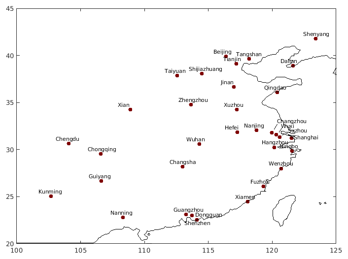
Figure 1Map of the 34 cities/urban clusters (population over 3 million, 2010 census) with available data (observational and model ensembles), used in this evaluation.
Within the EU projects MarcoPolo and Panda, a number of chemistry-transport models have been applied to provide daily air quality forecasts for a selection of 37 large Chinese agglomerations (population over 3 million, 2010 census). Initially, seven models, CHIMERE (Royal Netherlands Meteorological Institute, KNMI), IFS (European Centre for Medium-Range Weather Forecasts, ECMWF), WRF-Chem-SMS (Shanghai Meteorological Service, SMS), SILAMtest (Finish Meteorological Institute, FMI), WRF-Chem-MPIM (Max Planck Institute for Meteorology, MPIM, in Hamburg), EMEP MSC-W (hereafter referred to as EMEP, Norwegian Meteorological Institute, MET Norway), and LOTOS-EUROS (the Netherlands Organisation for applied scientific research, TNO) were providing daily forecasts every day at 00:00 UTC for the next 72 h (3 days) for NO2, O3, PM10, and PM2.5 (see Fig. 1). WRF-CMAQ and WRMS-CMAQ, both used by Chinese institutions (Nanjing University and SMS), have recently joined the prediction system, but are not considered in the present analysis.
We should note that the models considered in the present study may have significantly evolved since the present analysis was performed. This is the case, for example, for the SILAM model developed by the Finish Meteorological Institute, whose configuration was still in a test mode and is therefore referred to as SILAMtest. Several of the models considered here have been involved in a previous intercomparison summarized by Bessagnet et al. (2016).
The individual models are executed independently on the computing systems available in each partner institution. The surface concentrations of the key chemical species are extracted locally from the model outputs and forwarded to a central database operated by the Royal Netherlands Meteorological Institute (KNMI).
Hourly predictions of surface concentrations (expressed in µg m−3) are provided by the models as grid values, which are bilinearly interpolated to city center coordinates. The average for the data provided by the urban network (usually around 5–12 stations), is posted together with the corresponding standard deviation and the number of contributing stations. In the present analysis, we only consider the model simulations corresponding to 34 cities, since the cities of Ürümqi (most western, only covered by three models), Changchun, and Harbin (most northern cities) are located outside of the domains covered by most individual models, which are indicated in the companion paper (Brasseur et al., 2019).
In addition to the forecasts provided by the individual participating models, a multimodel ensemble was constructed from which the median and the mean were derived. To process the ensemble median, all seven individual models are first interpolated to a common horizontal grid. For each grid point, the ensemble model is calculated as the median value of the individual model forecasts. The median is relatively insensitive to outliers in the forecasts. The method is also less vulnerable to occasionally missing data from individual models, as the minimum number of model results needed to calculate a meaningful ensemble mean or median is almost always available. This will be discussed in detail in Section 4. The multimodel approach also provides more accurate forecasts and thus reduces the underlying uncertainties (as will be shown in the following section). More advanced methods, e.g., based on individual model skills, are discussed in the literature (e.g., Galmarini et al., 2013). They are significantly more costly from a computational point of view and therefore not well suited for daily operations.
The evaluation of the performance of a forecasting system is a necessary step for assessing the quality of the predictions and demonstrating its usefulness. It also provides important information that can lead to the improvement of the forecasting system and to further model development. The comparison between model output and in situ measurements is not straightforward because of the different nature of the respective quantities: air quality models provide volume-averaged quantities over each model grid cell and time averages over the modeling time step. Observations are available at fixed measurement sites and at a fixed time. Further, they are influenced by local processes that are not necessarily well captured by relatively coarse-resolution models. Thus, the representativeness of the observational site is not always guaranteed.
The MarcoPolo–Panda forecasting and analysis system uses the surface observations available at the web site http://www.pm25.in for 37 Chinese cities. For a given city, the observational data considered for the evaluation of the model consist of an average of the measurements made at the different stations of the urban network, usually 5–12 stations, which are aggregated to one value for the whole city. The model fields are bilinearly interpolated to the city center coordinates.
The mean bias,
where mi and oi are the model forecast value and the observation value, and N the number of model–observation pairs; the root mean square error,
the modified normalized bias,
the fractional gross error,
and the correlation coefficient between the model forecast and observed values,
are used to measure the system performance. Here and are the mean values of the model forecast and observed values, and σm and σo are the corresponding standard deviations.
The evaluation presented here aims to investigate (a) the statistical indicators for each model over the time of the year (on a monthly basis) so that the seasonal features can be characterized and related issues of individual models can be identified (Sect. 3.1); (b) the geographical distribution of the statistical indicators of the ensemble median to highlight regional characteristics and related issues (Sect. 3.2); (c) statistical indicators of all models and the ensemble median over the time of the day (considering all model–observation pairs of all cities and for the whole time period) and for a specific city (Beijing) together with the diurnal variation in the pollution species over the whole time period (Sect. 3.3).
3.1 Evaluation of the seasonal behavior of the models
We start our evaluation of the multimodel prediction system by examining the seasonal behavior of the predicted concentrations of key chemical species. The statistical indicators mentioned above have been calculated separately for each month from April 2016 to June 2017 and for the entire period during which the forecasting system was operational. Due to storage issues, only the predictions for the first 24 h (0–23 h) were saved while the predictions from 24 to 72 h were not retained and not analyzed in this work.
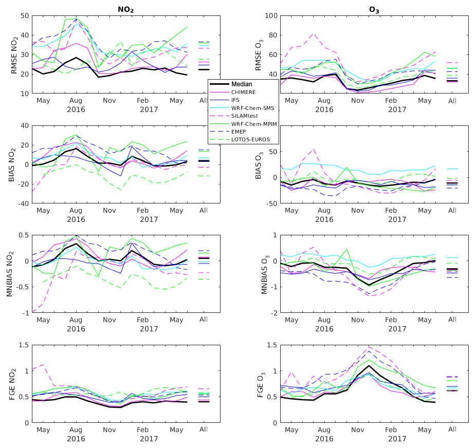
Figure 2RMSE (in µg m−3), BIAS (in µg m−3), MNBIAS, and FGE of NO2 and O3 for each month and for the entire time period (April 2016–June 2017 and lines on the right side of each panel).
Figure 2 shows the RMSE, BIAS, MNBIAS, and FGE of NO2 (left column) and O3 (right column) for each of the seven individual models included in the system, for the model ensemble median, and for each individual month between April 2016 and June 2017. The same results are also provided for the whole period (“All”). It can be seen that there is a wide spread of the results produced by the seven models. The individual models are continuously improving during the first months because many changes have been applied by the different modeling groups in order to improve their individual predictions. In the case of NO2, most individual models slightly overestimate the concentrations compared to observations. In the EMEP model, it may be explained by the larger nitrogen emissions used in comparison with the other models (Brasseur et al., 2019). This results in a positive BIAS and MNBIAS for most models and the ensemble median. The RMSE of the model ensemble is highest in July/August/September 2016 and remains relatively constant after October 2016. It can be seen that the median of the model ensemble has the lowest RMSE for NO2, the smallest BIAS and MNBIAS (slightly positive) and the lowest FGE. This demonstrates the advantage of adopting a model ensemble rather than the prediction provided by individual models.
Most models underestimate O3 (likely as a result of the overestimated NO2 because the O3 production is not NOx-limited) during the whole period under consideration. For O3, the CHIMERE model shows slightly better performance (lowest RMSE) than the model ensemble median. The median BIAS for O3 is relatively constant (slightly negative). For this particular species, the model ensemble median does not provide the best results regarding the BIAS. In fact, in this case, the model LOTOS-EUROS gives the best performance for ozone, Interestingly, this particular model has the largest negative BIAS for NO2. The median BIAS of O3 remains relatively constant during the period, while the MNBIAS exhibits higher negative values during the winter months, as a result of the relatively low O3 concentrations during wintertime.
As stated above, the MarcoPolo–Panda prediction system has the tendency to overestimate surface NO2, which leads to O3 titration especially during nighttime. The emission injection height is also a relevant factor here since it can largely influence the results in the planetary boundary layer. During night-time, emissions from stacks may take place above the mixing layer and explain model–data discrepancies since the models often assume that the injection of primary pollutants takes place in the first layer above the surface.
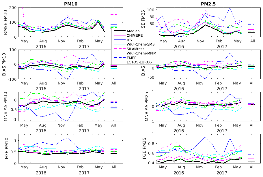
Figure 3RMSE (in µg m−3), BIAS (in µg m−3), MNBIAS, and FGE of PM10 and PM2.5 for each month and for the entire time period (April 2016–June 2017 and lines on the right side of each panel).
Anthropogenic emissions of primary pollutants are changing extremely rapidly in China. The adopted emissions inventories usually reflect the situation a few years before the period during which the model simulations were performed. Since the recent NOx emissions have decreased significantly in some urban areas of China in response to measures taken by the local authorities (Liu et al., 2017), the anthropogenic emissions used for the current forecasts may be overestimated in some areas. Some models use reduced NOx and SOx anthropogenic emissions (for details see Brasseur et al., 2019); however, daytime concentrations of ozone are generally underestimated in most models, even when the level of NO2 is in reasonable agreement with the observational values. The discrepancy could be caused by an underestimation of the emissions of some VOCs, especially in the center of urban areas where ozone is often VOC-limited.
For PM10 and PM2.5, the model ensemble median shows the best performance compared to all individual models during the time period under consideration (see Fig. 3). For PM10, there is an overall slight underestimation by all models except by CHIMERE and hence by the median of the model ensemble. For PM2.5, the BIAS is relatively constant (apart in the WRF-Chem-SMS model which exhibits a lot of variation in the BIAS of PM10 and PM2.5). In this case, the BIAS is slightly overestimated but close to zero.
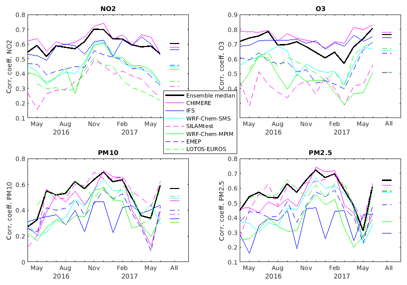
Figure 4Correlation coefficients based on hourly concentrations of NO2, O3, PM10, and PM2.5 for each month between April 2016 and June 2017 (and for the entire time period, lines on the right side of each panel).
Figure 4 shows the temporal correlation coefficients for NO2, O3, PM10, and PM2.5 for each individual month, and for the whole time period. It can be seen that there is a wide spread between the individual models: the calculated correlations range from 0.2 to 0.7 for NO2, PM10, and PM2.5, and from 0.3 to 0.8 for O3. The model ensemble median and CHIMERE are characterized by high correlation coefficients in the case of NO2, O3, and PM2.5. For PM10, the model ensemble median and the LOTOS-EUROS model provide the highest correlation coefficients. In general, the model ensemble median gives the best performance.
The correlation coefficient of O3 for the ensemble median on the monthly basis remains relatively unchanged between April 2016 and June 2017, and ranges between 0.6 and 0.8. Considering the whole time period, it is on the order of 0.75, with CHIMERE providing a slightly higher correlation coefficient for the whole time period, and also for each individual month. All models exhibit low correlation coefficients in March 2017. High correlation coefficients are found during the early summer months (June/July). For PM10 and PM2.5, the correlation coefficients exhibit more variability, starting with very low correlations for all models and for the ensemble during April and May 2016, high correlations from June 2016 to March 2017, and again low correlations during April and May 2017. These differences may be due to missing sources of biomass burning or dust or to individual model tunings. An important difference between the models included in the ensemble is the formulation of dust mobilization (see Table 3 of the companion paper by Brasseur et al., 2019). Note that the CHIMERE and EMEP models do not include dust in their calculation of particulate matter and that the emissions provided by the IFS-ECMWF are substantially higher than in other models. For the entire time period, the correlation coefficient of the ensemble mean is higher than for each individual models (∼0.58 for PM10 and ∼0.78 for PM2.5). The correlation between the model ensemble and the observations is therefore relatively satisfactory.
3.2 Evaluation of the geographical distribution
The statistical indicators, described above for all contributing cities, have also been calculated for the individual cities. The purpose here is to assess regional characteristics and to identify model issues. Figure 5 shows the statistical indicators (RMSE, BIAS, and correlation coefficient) for O3, NO2, and PM2.5 of the ensemble median for each city during the time period under consideration (April 2016 until June 2017). In the uppermost left panel, the BIAS of ozone for each city is shown. It can be seen that the ensemble median is underestimating the ozone concentrations in the north and northeastern regions of China, while no significant bias compared to the observations is found in cities in the southern part of the country. RMSE in the northern and northeastern cities are higher (around 40 µg m−3) than in southern and western cities (around 20–30 µg m−3).
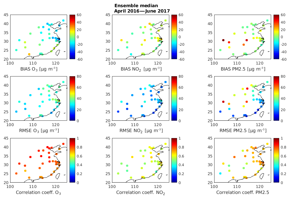
Figure 5Map of the BIAS, RMSE, and temporal correlation coefficient of O3, NO2, and PM2.5 for the whole time period (April 2016 until June 2017) for each city.
The temporal correlation coefficients for ozone calculated for each city over the whole period under consideration are slightly higher in the northern part of the country and slightly smaller in the southern regions. This indicates that the day-to-day variability is well simulated, even though the models are slightly underestimating the ozone pollution in the north. NO2 concentrations (see the middle row panels of Fig. 5) are overestimated in some cities and underestimated in other cities. There is, however, no systematic geographical characterization of the bias. When considering individual cities, it can be seen that the NO2 concentrations are slightly overestimated in most urban areas including Beijing, Shanghai, Chengdu, Wuhan, and Changsha. The missing urban parameterization could be one of the reasons for too low vertical mixing in the model. The RMSE for NO2 in the middle panel of Fig. 5 is very uniform (around 20 µg m−3) in the whole country. The correlation coefficients of NO2 (between 0.5 and 0.7) are smaller than those of O3 as NO2 exhibits more temporal variability than O3. In the case of PM2.5, (see uppermost right panel), the concentrations are well simulated in the northern and southern parts of China, but there are a few city clusters in the middle of the domain (Chengdu, Chongqing, Wuhan, and Changsha) in which the PM2.5 concentrations are overestimated by more than 50 µg m−3. These cities also show an overestimation of NO2 concentrations. The overestimation of PM2.5 may therefore be related to the errors in precursor emissions, e.g., NOx and SO2. The RMSE of PM2.5 is smaller in the southern part of the domain and along the coastline of China, while the model results are less satisfactory in the city clusters located in the central part of the domain, with very high RMSE of 60–80 µg m−3 in three cities. The correlation coefficients for the individual cities are relatively constant around 0.7 with few cities characterized by lower correlation coefficients (mostly in the central part of the domain).
3.3 Evaluation of the diurnal variation
We now examine the ability of the models to reproduce the diurnal variations of the chemical species' concentrations. We first provide a general view based on all observations in China and then examine the particular situation in the city of Beijing.
3.3.1 Analysis based on all observations in China
The RMSE, BIAS, MNBIAS, and FGE of O3, NO2, PM10, and PM2.5 for the seven models and the ensemble median for all available observations in China are displayed over the forecasting time (0–23 h; Figs. 6 and 7). Due to storage limitations, only the predictions for the first 24 h (0–23 h) were saved while the predictions for the 24–72 h period performed by all models were not retained. Unfortunately, this does not allow the investigation of a day-to-day degradation of the statistical indicators (from day 1 to day 3). Only the diurnal behavior of the statistical indicators can be assessed, which provides important hints for possible model issues.

Figure 6RMSE, BIAS, MNBIAS, and FGE of NO2 and O3 over the forecasting time (time of the day).

Figure 7RMSE, BIAS, MNBIAS, and FGE of PM10 and PM2.5 over the forecasting time (time of the day).
It can be seen in the left column of panels of Fig. 6 that the statistical indicators of NO2 for the ensemble median is relatively stable over the time of the day, with slightly higher RMSE and higher BIAS/MNBIAS during the nighttime hours. For the individual models, the variability in the RMSE is somewhat higher during daytime, while some models exhibit very high RMSE and BIAS during the nighttime hours. Most models show a positive BIAS of NO2 during the night, but a few of them exhibit a negative bias; this results in a relatively small BIAS for the ensemble median, showing good results with respect to the BIAS throughout the day.
In the case of ozone, the statistical indicators exhibit a variation over the time of the day. The RMSE is smallest between 07:00 and 09:00 LT (local time), after which it increases until 18:00 LT in the evening to become constant at about 30 µg m−3 during the night.
An examination of the BIAS and MNBIAS for O3 over the day shows that O3 is underestimated by nearly all models, apart from WRF-Chem-SMS. This might result from the slight overestimation of NO2 concentrations by most models. Especially during nighttime when the height of the boundary layer is low, near-surface NO2 concentrations are high, and ozone is underestimated by 50 %–100 % by most models. In the first hours of the day, only SILAMtest, WRF-Chem-SMS, and LOTOS-EUROS exhibit slightly positive O3 BIAS. The same models produce a negative BIAS for NO2 during the first hours of the day.
Figure 7 shows that the BIAS and MNBIAS of both PM10 and PM2.5 stay relatively constant over the time of the day. PM10 is slightly underestimated by the ensemble median (−5 % to −10 %), while PM2.5 is slightly overestimated (10 % to 25 %). In most cases, the models overestimate the PM2.5 observations, while for PM10 there are stronger differences between the individual models.
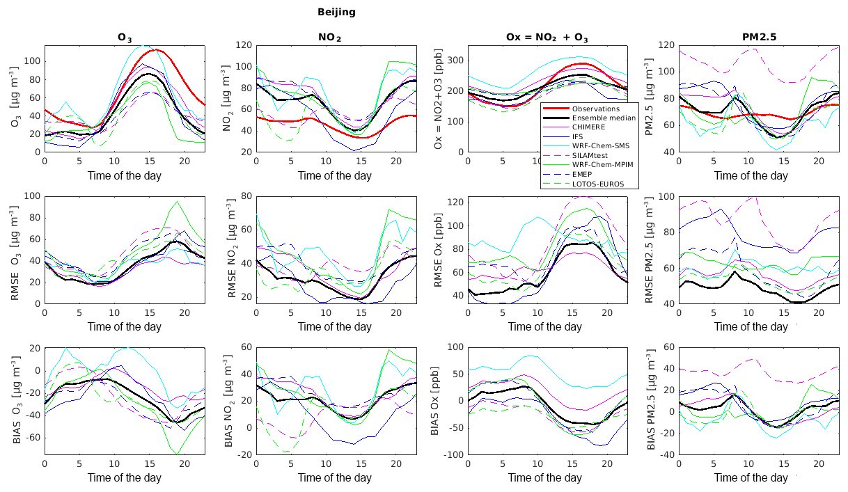
Figure 8Diurnal variations in the concentrations and of the RMSE and BIAS of O3, NO2, Ox, and PM2.5 for Beijing for the whole time period (April 2016–June 2017).
For PM10 and PM2.5, the ensemble median exhibits a better performance than the individual models: the RMSE BIAS, MNBIAS, and FGE of the ensemble are on average lower than the corresponding statistical parameters of the individual models. This demonstrates again the advantage of using the ensemble median for the prediction of PM10 and PM2.5.
Figure 8 presents the diurnal variation in the concentrations of O3, NO2, O3+NO2, and PM2.5 from the individual models (and the ensemble median) and from the observations at a specific location (Beijing). The RMSE and the BIAS are also provided during the whole period under consideration.
It can be seen that the ensemble median (black line) underestimates the O3 observations (red line) throughout the day, especially during the nighttime hours and in the late afternoon. Only WRF-Chem-SMS reproduces the amplitude of the O3 diurnal cycle, but it also underestimates the O3 concentrations after 18:00 LT when the height of the boundary layer is rapidly decreasing. All models and the ensemble median reproduce the diurnal cycle with a maximum in the late afternoon, but this maximum produced by the model appears about 2 h earlier than observed. When considering the RMSE, the models produce the best results during the morning, and with increasing O3 concentrations as the day progresses; the RMSE is also increasing. The negative BIAS is increasing for all models and for the model ensemble throughout the day.
3.3.2 Analysis for the specific case of Beijing
In Beijing, the diurnal variation in the NO2 concentrations is overestimated by the individual models as also reflected by the ensemble median. During the nighttime, for example, the observed concentrations are about 20–30 µg m−3 lower than the concentrations associated with the ensemble median. The individual models and the ensemble median show a much stronger diurnal behavior than the observations. Atmospheric measurements suggest that the concentrations of NO2 are relatively constant over the time of the day. This might be due to applied temporal profiles of the anthropogenic emissions or issues in the vertical mixing of the individual models. Also, the models with their spatial resolution may not capture the details seen in the observations by the ground network. The RMSE of all models and for the ensemble median is highest in late afternoon and during the night. The MarcoPolo–Panda prediction system has thus a tendency to overestimate surface NO2, which leads to an overestimation of the O3 titration especially at night.
To further analyze the chemical coupling between ozone and NO2, we have added, at each time step, the mixing ratios of O3 and NO2. The resulting variable, called Ox and expressed here in ppbv, has the advantage of not being affected by the fast interchange (null cycle) and the resulting partitioning between ozone and NO2 produced by reactions NO+O3, NO2+hν, and . If only these three rapid photochemical reactions are considered, Ox is a conserved quantity. In other words, even when a more comprehensive chemical scheme is adopted, the diurnal cycle of Ox should be considerably less pronounced than the diurnal cycle of NO2 and O3.
In fact, in the model forecasts, the sum of O3 and NO2 is nearly constant during the day, but exhibits nevertheless some diurnal variation, which appears to be weaker than in the observation. The calculated Ox is slightly too high at night and too low during daytime, suggesting an overestimation in photochemical activity by the majority of the models. The partitioning of Ox into NO2 and O3 is not well reproduced despite the simple chemistry that determines this partitioning: NO2 is generally too high and O3 too low, especially in the afternoon and early night. The simple partitioning approach does not seem to work properly under high NOx loading. As a result, the diurnal cycle of O3 is not well reproduced by the forecasting ensemble and high ozone events are generally underestimated. This issue is discussed in more detail in the companion paper by Brasseur et al. (2019).
The observed diurnal variation in PM2.5 is not well reproduced by the models and by the ensemble median. The calculated variability in Beijing is substantially higher than suggested by the observations (which are characterized by relatively constant concentrations throughout the day). The models show a maximum in PM2.5 concentrations around 08:00–09:00 LT, and a second maximum during nighttime hours. This morning maximum is not present in the observations. The model ensemble is overestimating the observations in the morning and underestimating them in the early afternoon, resulting in a diurnal variability in the BIAS, shown in the lowest panel. Again, this might be related to the adopted diurnal profiles of the anthropogenic emission sources or might be due to errors in the formulation of vertical mixing in the planetary boundary layer. Specifically, one should note that the models do not include a detailed formulation of small-scale urban canopy effects, which could generate some mechanical and thermal turbulence with related vertical mixing during nighttime. With increased nighttime ventilation from the boundary layer to the free troposphere, the calculated amplitude of the diurnal variation in gases and particulates would be reduced and become closer to the observation.
To assess the impact on the ensemble forecast of occasionally missing results from one or several models, we compare the following ensembles during a given test period (1–30 May 2017), separately for O3, NO2 and PM2.5: this approach has already been adopted by Marécal et al. (2015) to evaluate European air quality predictions. We consider the following cases:
-
MEDIAN 7. the median provided by the operational ensemble method, which includes all seven models;
-
MEDIAN 5. the median built on five individual models, excluding the “best” and the “worst” models;
-
MEDIAN 3. the median built on three individual models, excluding the two “best” and the “two” worst models;
-
BEST. the model with the highest performance;
-
WORST. the model with the lowest performance.
Since the relative performance of individual models varies in time and space, the criterion to order the seven individual models from “worst to best” is provided by the value of their respective RMSE over the test period. For ozone, the criterion is measured by the RMSE over the 30 days between 12:00 and 18:00 LT (ozone peak time) (this criterion is based on the fact that the “best” model refers to the best forecast of daytime ozone levels). RMSE is seen as the most objective criterion since mean bias and modified normalized bias can include compensating effects.
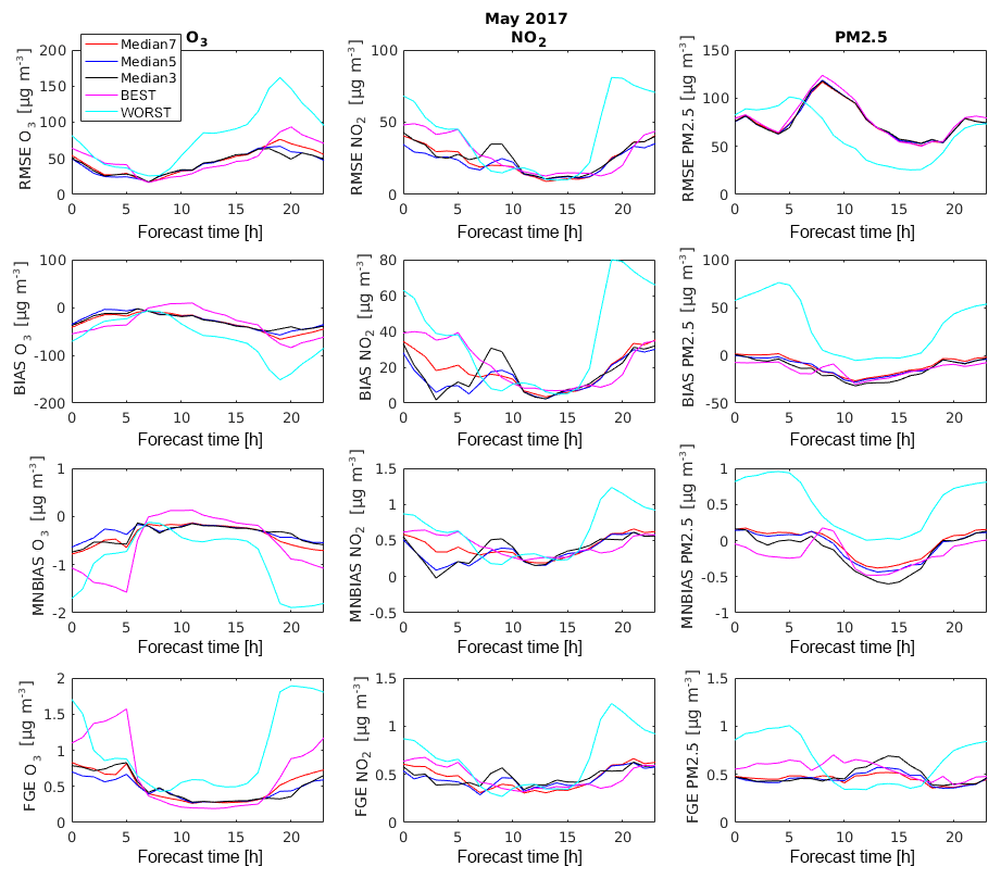
Figure 9RMSE, BIAS, MNBIAS, and FGE of O3, NO2, and PM2.5 over the forecasting time (time of the day) for the Median7, Median5, Median3, and the best and worst model.
Figure 9 shows the statistical indicators for May 2017 as a function of the forecasting time (0–23 h) of the ensemble median based on all seven models (MEDIAN7 shown in red), five models (MEDIAN5 shown in blue), and three models (MEDIAN3 shown in black). The results are also shown for the “best” and the “worst” model (BEST, magenta, and WORST, light blue). For all three species, the ensemble median based on seven models is of highest quality (based on the statistical indicators used in this analysis), and generally surpasses the results provided by the “best” model. When only five models (excluding the best and the worst) are available to calculate the ensemble, all statistical indicators show only very small differences with the more inclusive MEDIAN7 case based on seven models. Reducing the ensemble calculation further to three models (MEDIAN3), the statistical scores degrade slightly compared to the MEDIAN7 and MEDIAN5 for all three species, but remain higher or at least similar to the score of the best model (BEST).
It is interesting to note that the best model (BEST) is not the same model for the different months that are investigated, nor the same model for all species. For example, in August 2016, the best model for O3 and PM2.5 is IFS, while LOTOS-EUROS shows the best performance for NO2. In May 2017, the best model for PM2.5 is LOTOS-EUROS and the worst model is IFS, but the results remain the same: the ensemble product performs better than (or at a similar level as) the best model. Since the BEST model can change depending on time period and species, the ensemble product is particularly valuable for the sustained quality of the forecasting system. This study shows, therefore, that using the ensemble product (median) of models, even if occasionally based on fewer models, is more useful than using a single model, even if the performance of this individual model is high. The ensemble product is still robust compared to the observations if the output of some contributing models is occasionally missing. It also shows that an ensemble product remains valuable even if only few models are available for the production of the forecast.
The prediction system has been designed to support the development of policies and the calculation of air quality indices. One of the applications of the system is to provide alerts to the general public when acute air pollution episodes are expected. Thus, the performance of the forecast system has been tested regarding the likelihood to predict air pollution events. We will refer to this type of forecast as binary prediction of events (Brasseur and Jacob, 2017).
A model prediction of a specific event such as an air pollution episode at a given location (e.g., concentration of pollutants exceeding a regulatory threshold) is evaluated by considering a binary variable and by distinguishing between four possible situations: (1) the event is predicted and observed, (2) the event is not predicted and not observed, (3) the event is predicted but not observed, (4) the event is not predicted but is observed. Cases (1) and (2) are regarded as successful predictions (hits), while (3) and (4) are considered to be failures (misses). The skill of the model for binary prediction (event or no event) is measured by the fractions of observed events that are correctly predicted (probability of detection, POD). The fraction of predicted events that did not occur is measured by the false alarm rate (FAR), both POD and FAR as defined in Brasseur and Jacob (2017).
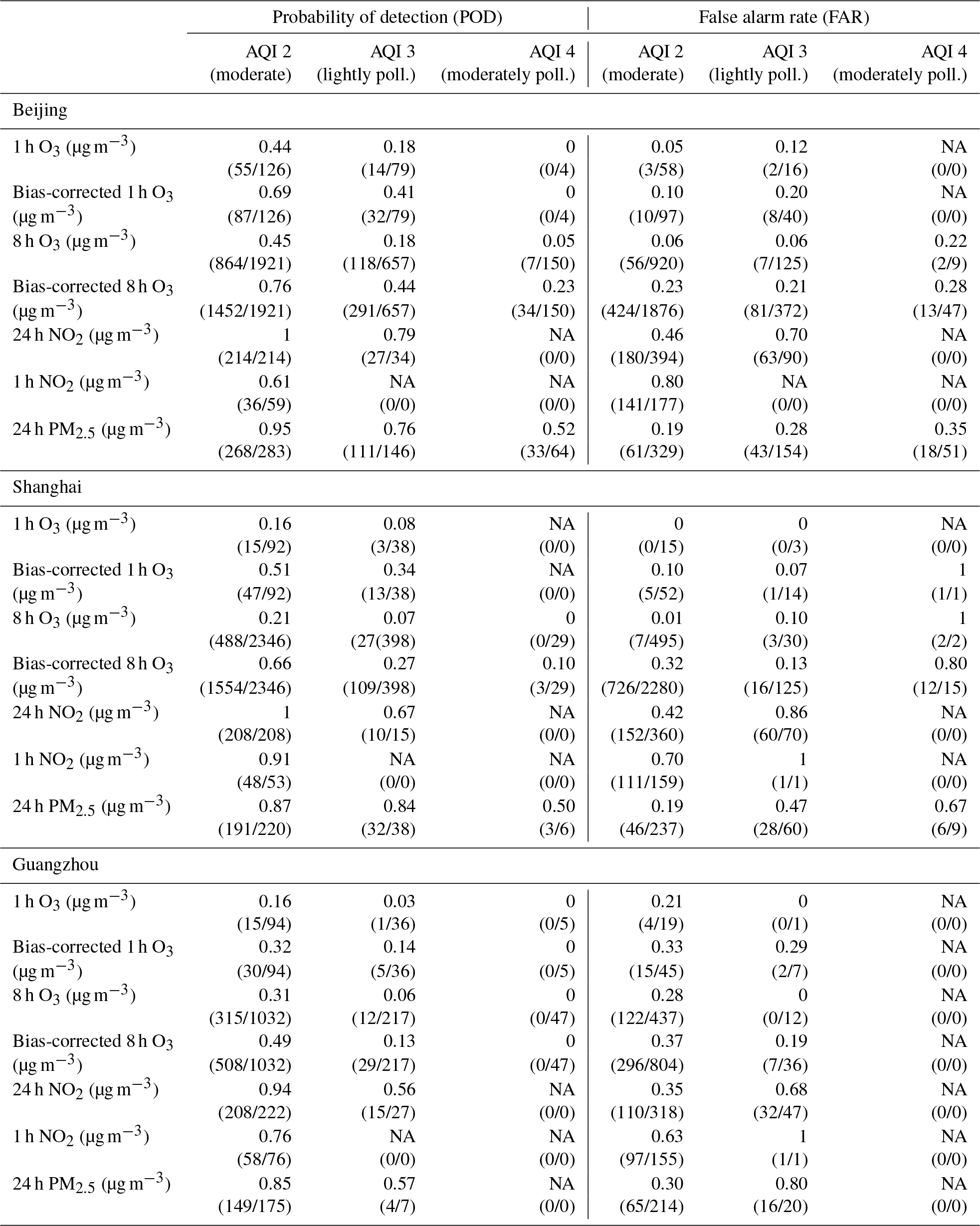
We have calculated the POD and FAR for the ensemble median for the cities of Beijing, Shanghai, and Guangzhou between April 2016 and June 2017, specifically for ozone (based on the 8 h and the daily maximum value), NO2, and PM2.5. Based on the 1-hourly time series of ozone, NO2 and PM2.5, the time series for (a) 1 h ozone, (b) 8 h ozone concentrations (c) 24 h mean NO2 concentrations, (d) 1 h NO2 concentrations, and (e) 24 h PM2.5 concentrations have been constructed and the thresholds of the air quality indices (AQI) have been applied for each definition. The definitions breakpoints for the individual AQI are shown in Tables 1 and 2; they are based on current definitions of AQI from the Chinese government.
In order to highlight the presence of thresholds violated during the time period under consideration, Figs. 10–12 show the time series for the period April 2016–July 2017 of the (1) daily maximum ozone concentrations, (2) 8 h moving average of ozone, (3) the 24 h mean NO2 concentrations, (4) the daily maximum NO2 concentrations, and (5) the 24 h mean PM2.5 concentrations for Beijing (Fig. 10), Shanghai (Fig. 11), and Guangzhou (Fig. 12) derived from the model and from the observations at each location. Pink lines indicate the thresholds for the air quality indices for moderate (line), lightly polluted (dashed line), and moderately polluted (dotted line) conditions for each pollutant.

Table 2Individual AQI (IAQI) for 1 and 8 h ozone, 24 and 1 h NO2, and 24 h PM2.5.
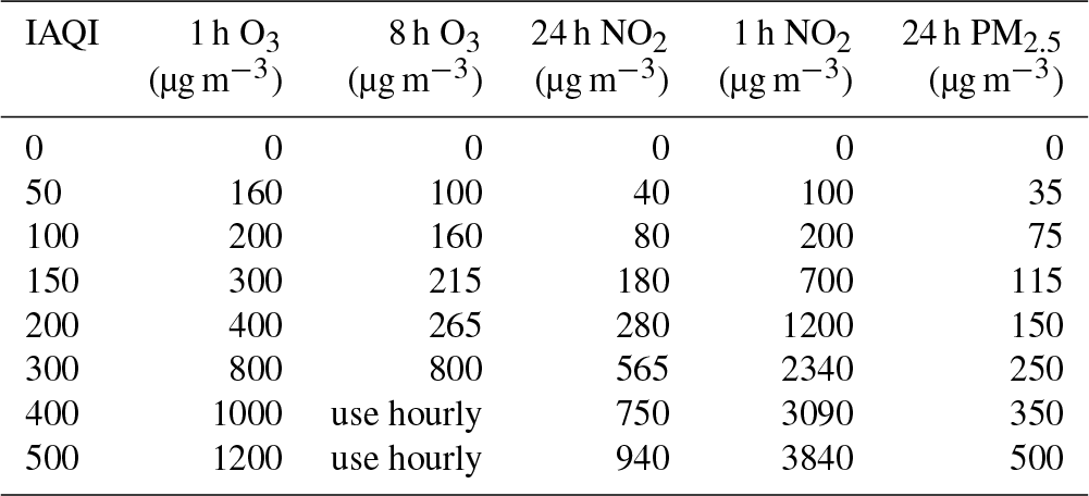
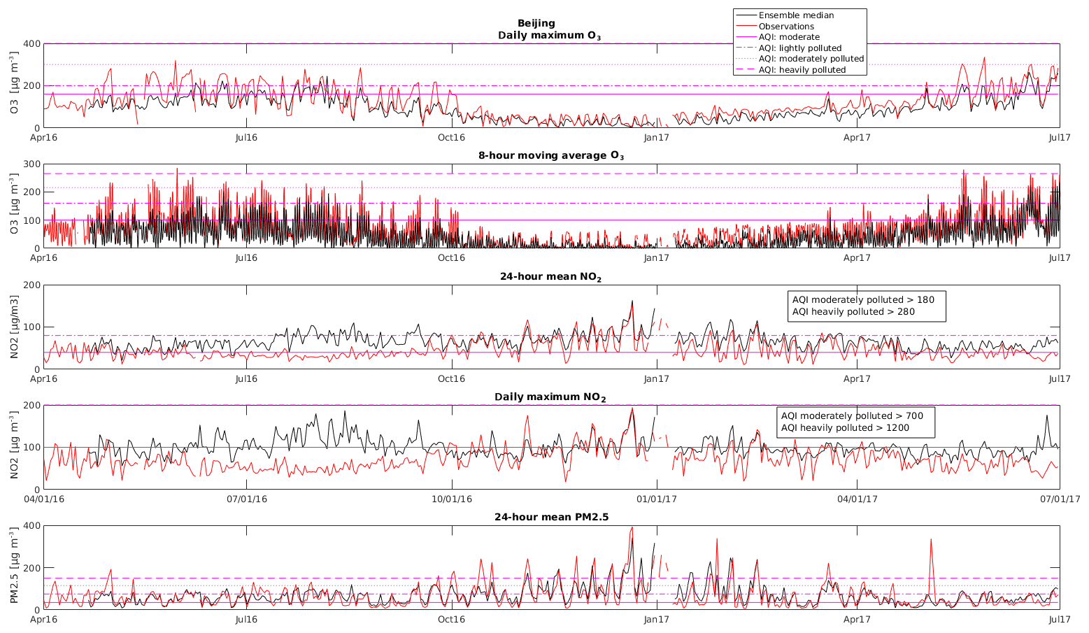
Figure 10Time series of daily maximum O3, 8 h moving average O3, 24 h mean NO2, daily maximum NO2, and 24 h mean PM2.5 for Beijing from April 2016 until June 2017.

Figure 11Time series of daily maximum O3, 8 h moving average O3, 24 h mean NO2, daily maximum NO2, and 24 h mean PM2.5 for Shanghai from April 2016 until June 2017.
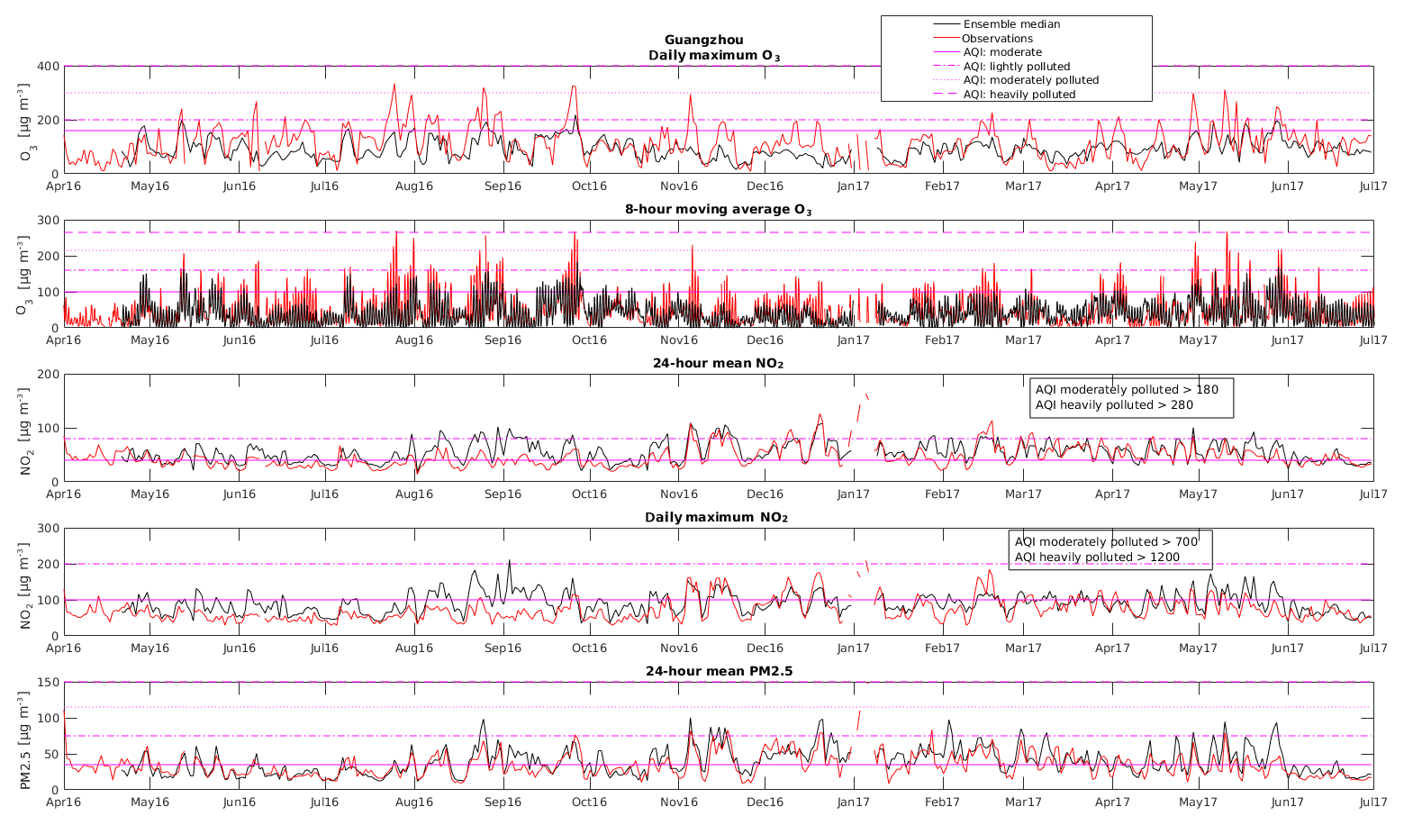
Figure 12Calculated (ensemble median) and observed time series of daily maximum O3, 8 h moving average O3, 24 h mean NO2, daily maximum NO2, and 24 h mean PM2.5 for Guangzhou from April 2016 until June 2017.
In Beijing and Shanghai, the daily maximum ozone concentrations exceeded the thresholds of 160 (moderate) and 200 (lightly polluted) within the considered time period only during the months of April to September 2016. During the months of October 2016 to March 2017, the ozone concentrations remained below the threshold of 160, highlighting fair air quality conditions with regard to ozone in wintertime. In Beijing, the ensemble median has a probability of detection of air pollution events for moderate 1 h ozone AQI of 0.44 (55 out of 126 events of 1 h ozone breaking the threshold of 160 µg m−3 have been detected). The FAR is 0.05; the model ensemble predicted 58 events where ozone exceeds the threshold of 160 µg m−3, where 3 out of these 58 events were false alarms (observations below the threshold). Lightly polluted events (1 h ozone exceeding 200 µg m−3) were correctly predicted only 14 times, while the observations exceeded the threshold 79 times. The FAR for lightly polluted ozone events is 0.12 (2 out of 16).
For moderately polluted ozone events (1 h ozone exceeding 300 µg m−3), the POD is 0; the model ensemble was not able to predict the four observed events (FAR is not applicable, 0 out of 0).
Looking at the 8 h ozone predictions for Beijing, the model ensemble is very similar, with a POD of 0.45 (864 out of the 1921 observed events have been predicted correctly) and a FAR of 0.06 (56 counts are false alarms out of 920 events). For lightly polluted ozone conditions, the POD is 0.18 (118 out of 657 observed events) with a FAR = 0.06 (7 out of 125 are false alarms). For moderately polluted conditions, the model ensemble predicted 7 out of 150 observed events correctly with a FAR of 0.22 (2 out of 9 alarms are false).
For Shanghai, the PODs for ozone predictions are lower than in Beijing: for moderate air quality conditions, the POD is 0.16 (15 out of 92 observed events are predicted correctly) with a FAR of 0 (no false alarm) for 1 h ozone predictions, and POD = 0.21 (488 out of 2346 observed events) with a FAR of 0.01 (7 false alarms relative to 495 counts) for 8 h ozone predictions. For lightly polluted conditions, the POD is decreasing: POD = 0.08 (3 correct predictions out of 38 observed events) with FAR of 0 (no false alarm, 3 correct predictions) for 1 h ozone, and POD = 0.07 (27 out of 398 observed) with a FAR of 0.10 (3 false alarms out of 30) for 8 h ozone. For moderately polluted conditions (1 h ozone exceeding 300 µg m−3 or 8 h ozone exceeding 215 µg m−3), the POD for 1 h ozone is not applicable (not predicted, no observed events), and for 8 h ozone POD = 0 (0 predicted out of the 29 observed), FAR = 1 (2 false alarms out of 2 predicted, but not observed).
In Guangzhou, there is no clear difference between ozone conditions in summer or wintertime during the considered time period. Ozone observations regularly exceed the threshold of 160 (moderate) and 200 µg m−3 (lightly polluted) during the whole time period, and five times 1 h ozone is exceeding the threshold of 300 µg m−3.
The POD of 1 h ozone in Guangzhou is 0.16 (15 correct predictions out of 94 observed) with FAR = 0.21 (4 false alarms out of 19 predicted) for moderate conditions, and POD = 0.03 (1 predicted out of 36 observed) with FAR = 0 (0 out of 1 predicted) for lightly polluted conditions, and POD = 0 (0 predicted out of 5 observed events) for moderately polluted ozone conditions. For 8 h ozone, the POD is 0.31 (315 correct predicted out of 1032 observed) with FAR = 0.28 (122 false alarms of 437 predicted events) for moderate conditions, POD = 0.06 (12 out of 217 observed) with FAR = 0 (no false alarm out of 12 predicted events) for lightly polluted ozone conditions, and POD = 0 (0 out of 47 observed events) for moderately polluted ozone conditions.
In general, the ability of the model ensemble to correctly predict ozone air pollution events is best for light ozone pollution, while it fails to predict correctly the ozone pollution events for moderately polluted situations. This is mostly a result of the model ensemble being too low compared to the observations. The predictions can be improved by applying a bias correction to the ozone predictions. This is investigated in the last section.
The NO2 predictions of the ensemble median are in general too high compared to the observations, especially in Beijing and Shanghai. Especially in summertime (June/July/August/September), the model predictions are sometimes twice as high as the observations, which might be a result of uncertainties in the emissions. In all three cities under consideration, the NO2 concentrations are only exceeding the thresholds of 40 µg m−3 for 24 h NO2 (100 for 1 h NO2) and 80 µg m−3 for 24 h NO2 (200 µg m−3 for 1 h NO2) during the considered period (moderate and lightly polluted conditions for NO2). During wintertime (November/December/January), the observations are slightly higher than in summer and the ensemble system is in better agreement with the observations.
In Beijing, the POD for 24 h NO2 is 1 (214 of 214 observed events are predicted) for moderate conditions with a FAR of 0.46 (180 false alarms relative to 394 predicted events). This indicates that NO2 is generally overestimated by the model ensemble. For lightly polluted events, the POD is 0.79 (27 predicted out of 34 observed events) with FAR = 0.70 (63 false alarms out of 90 predicted). For the 1 h NO2, the POD for moderate conditions is 0.61 (36 out of 59 observed events) with FAR = 0.80 (141 false alarms out of 177 predicted). For lightly polluted conditions, no events have been observed nor predicted for 1 h NO2 in Beijing during the considered period. In Beijing, the threshold for moderately polluted NO2 conditions has not been exceeded neither by 1 h NO2 nor by 24 h NO2 during the considered period.
In Shanghai, the numbers are very similar to those in Beijing: POD for 24 h NO2 is 1 (208 of 208 observed events are predicted) for moderate conditions with a FAR of 0.42 (152 false alarms of 360 predicted events). There is also a general overestimation by the model ensemble compared to the observations. For lightly polluted conditions, the POD for 24 h NO2 is 0.67 (10 out of 15 observed) and a FAR of 0.86 (60 false alarms of 70 predicted), which is a clear result of the overestimated NO2. For the 1 h NO2, the POD is 0.91 (48 predicted out of 53 observed) with a FAR of 0.70 (111 false alarms out of 159 predicted) for moderate conditions. The thresholds for lightly polluted and moderately polluted conditions for 1 h NO2 have not been exceeded in Shanghai during the considered period, but there was 1 false alarm (1 out of 1) for lightly polluted conditions.
In Guangzhou, the model ensemble and the observations for NO2 are in better agreement. There is slight overestimation of the NO2 concentrations from May to September 2016, and in May 2017, but in general, there is a good agreement between the model time series and the observations. The POD for 24 h NO2 exceeding the threshold for moderate conditions is 0.94 (208 predicted out of 222 observed) with a FAR of 0.35 (110 false alarms of 318 predicted events), for lightly polluted conditions POD is 0.56 (15 predicted out of 27 observed) with 32 false alarms out of 47 predicted events (FAR = 0.69). Stronger polluted events have not been observed nor predicted for NO2 in Guangzhou. For the 1 h NO2, 58 events have been predicted out of 76 observed for moderate conditions (POD = 0.76, FAR = 0.63; 97 false alarms out of 155 predicted). For lightly polluted conditions there was 1 false alarm (1 out of 1), with no observed nor predicted events.
The thresholds for moderately polluted conditions for 24 h NO2 and 1 h NO2 have not been exceeded in Guangzhou during the considered period, no events have been predicted nor observed.
The predictions of PM2.5 concentrations (24 h PM2.5) of the model ensemble are in very good agreement with the observations in all three cities during the considered period.
In Beijing, the POD for the prediction of moderate condition for 24 h PM2.5 is 0.95 (268 correctly predicted events out of 283 observed) with a FAR of 0.19 (61 false alarms out of 329 predicted events). For lightly polluted conditions, the POD is 0.76 (111 correctly predicted events of 146 observed events) with a FAR of 0.28 (43 false alarms for 154 predicted events). Moderately polluted PM2.5 events have been correctly predicted 33 times out of 64 observed events (POD = 0.52) with a FAR of 0.35 (18 false alarms out of 51 predicted events).
In Shanghai, 191 moderate pollution events for PM2.5 have been correctly predicted out of 220 observed events (POD = 0.87, FAR = 0.19), with 46 false alarms out of the 237 predicted events. For lightly polluted events, the POD is 0.84 (32 out of 38 observed events) with a FAR of o.47 (28 false alarms of 60 predicted events). For moderately polluted conditions of PM2.5, the POD is 0.50 (3 correctly predicted events out of 6 observed) with a relatively high FAR (0.67, 6 false alarms out of 9 predicted).
In Guangzhou, the POD for moderate conditions of PM2.5 is 0.85 (149 correctly predicted out of 175 observed) with 65 false alarms out of 214 predicted events (FAR = 0.30). Lightly polluted events have been observed only seven times, the ensemble median predicted four of them correctly (POD = 0.57), but with a very high false alarm rate (16 false alarms out of 20 predicted events, FAR = 0.80); this indicates a slight overestimation of the PM2.5 concentrations of the models compared to the observations. In Guangzhou, no moderately polluted events of PM2.5 have been observed nor predicted during the considered period.
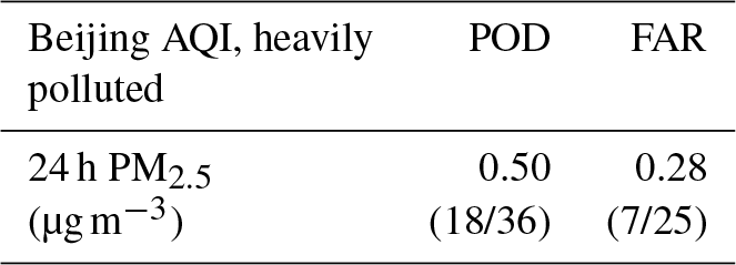
Only in Beijing, and only with regard to 24 h PM2.5, heavily polluted conditions have been observed and predicted during the considered period in the winter months 2016/2017 (see Table 4): the POD is 0.5 (18 correctly predicted out of 36 observed events) with a FAR of 0.28 (7 false alarms out of 25).
These investigations show that the model ensemble is well suited to be used in air quality predictions of PM2.5. For ozone, due to biases of the model ensemble compared to observations, the model ensemble is not able to predict ozone pollution in an appropriate way. Although the FAR is very low for ozone predictions, the POD of model ensemble is not very high. In the following section, we apply bias correction to improve the predictions for ozone pollution events.
Bias correction for ozone predictions
Bias corrections can be applied to improve the predictions of an individual model or a model ensemble. In our case, we have calculated the summertime bias of the time series of the hourly ozone concentrations from the model ensemble with respect to the hourly observations, and subtracted the bias from the hourly time series. For predictions of ozone air pollution, the summertime is an appropriate season to consider since the ozone thresholds are exceeded only during this season. As the bias between the observations and the model might not be the same for each month, and our goal is to obtain the best improvement in the ozone predictions for summertime, we have subtracted the mean summertime bias (mean of the bias of June/July/August/September 2016) from the original time series. The daily maximum ozone values and the 8 h moving average for the corrected time series have then been calculated. The resulting POD and FAR for 1 h ozone and 8 h ozone under different air quality conditions are shown in Table 3. This table shows that, for bias-corrected predictions, the POD in all three cities is larger than for the noncorrected time series, especially in the case of moderate and lightly polluted conditions of ozone. Thus, the predictions of air pollution events are significantly improved when the bias correction is applied in the case of ozone. Only for the predictions of moderately polluted conditions of ozone, the POD is not changing. The FAR is also slightly decreasing for all cities, but the improvement is small.
In Beijing, the POD air pollution events represented by a moderate AQI for 1 h ozone increased from 0.44 for Beijing (55 out of 126 observed events) before bias correction to 0.69 (87 out of 126 events) after bias correction. The FAR also increased from 0.05 (3 false alarms out of these 58 events) to 0.10 (10 false alarms out of 97 predicted events). Lightly polluted events (1 h ozone exceeding 200 µg m−3) have been predicted correctly 31 times (14 times without the corrections), while the observations exceeded the threshold 79 times. The FAR for lightly polluted ozone events also slightly increased from 0.125 (2 out of 16) to 0.2 (8 false alarms out of 40).
For moderately polluted ozone events (1 h ozone exceeding 300 µg m−3), the POD for the bias-corrected prediction is still 0. The model ensemble was not able to predict the 4 observed events (FAR is not applicable, 0 out of 0).
Table 4POD and FAR for PM2.5 for Beijing under heavily polluted conditions.
Looking at the 8 h ozone predictions for Beijing, the POD of 0.45 (864 out of the 1921 observed events have been predicted correctly) increased to 0.76 (1452 out of 1921) after bias corrections, and the FAR from 0.06 (56 counts are false alarms out of 920) to 0.23 (424 false alarms out of 1876 predictions) for moderate ozone pollution. For lightly polluted ozone conditions, the POD increased to 0.44 (291 out of 657) and FAR is 0.22 (81 false alarms of 372 predicted) for the bias-corrected predictions compared to POD is 0.18 (118 out of 657 observed events) with a FAR is 0.06 (7 out of 125 are false alarm). For moderately polluted conditions, the model ensemble with bias-corrected predicted 27 (instead of only 7) out of 150 observed events correctly with a FAR of 0.28 (13 false alarms of 47 predictions) compared to FAR of 0.22 (2 out of 9 are false alarm).
For Shanghai, for moderate air quality conditions of ozone, the POD increased from 0.16 to 0.51 (47 – 15 for noncorrected – out of 92 observed events are predicted correctly); the FAR increased from 0 (no false alarm) to 0.10 (5 false alarms out of 52) for 1 h ozone predictions. For 8 h ozone predictions, the POD increased from 0.21 to 0.66 (1554 – noncorrected: 488 – out of 2346 observed events), the FAR increased from 0.01 (7 false alarms of 495 predicted events) to 0.32 (726 false alarms of 2280 counts) for 8 h ozone predictions. For lightly polluted ozone conditions, the POD increased from 0.08 (3 correct predictions out of 38 observed, with FAR of 0; no false alarm, 3 correct predictions) to POD is 0.34 (13 out of 38) with FAR is 0.07 (1 false alarm of 14 predicted events) for 1 h ozone, and for 8 h ozone, the POD increased from 0.07 to 0.27 (109 – noncorrected: 27 – out of 398 observed) and the FAR increased from 0.10 (3 false alarms out of 30) to 0.13 (16 false alarms in 125 predicted events). For moderately polluted ozone conditions, the POD for 1 h ozone is not applicable for both noncorrected and bias-corrected predictions (not predicted, no observed events); but for the bias-corrected prediction, one false alarm is observed (FAR = 1, 1 false alarm in 1 predicted event), and for 8 h ozone POD increased from 0 to 0.10 (3 – noncorrected: 0 – predicted out of the 29 observed), the FAR decreased from 1 (2 false alarms out of 2 predicted, but not observed) to 0.8 (12 false alarms of 15 predicted events).
In Guangzhou, the predictions are not as accurate as in Beijing and Shanghai, and the bias corrections result only in slight improvements of the ozone forecasts for Guangzhou. The POD of 1 h ozone in Guangzhou increased from 0.16 to 0.32 (30 – noncorrected: 15 – correct predictions out of 94 observed) and the FAR slightly increased from 0.21 (4 false alarms out of 19 predicted) to 0.33 (15 false alarms out of 45 predicted events) for moderate conditions. For lightly polluted ozone conditions, the POD increased from 0.03 to 0.14 (5 – non corrected: 1 – predicted out of 36 observed) and the FAR increased from 0 (0 out of 1 predicted) to 0.29 (2 false alarms of 7 predicted events). For moderately polluted ozone predictions, the POD and FAR did not change with bias corrections (POD = 0 – 0 predicted out of 5 observed events – FAR not applicable).
For 8 h ozone of moderate conditions, the POD increased from 0.31 to 0.49 (508 – noncorrected: 315 – correct predicted out of 1032 observed) and the FAR increased from 0.28 (122 false alarms of 437 predicted events) to 0.37 (296 false alarms for 804 predictions). For lightly polluted ozone conditions the POD increased from 0.06 to 0.13 (29 – noncorrected: 12 – out of 217 observed) and the FAR increased from 0 (no false alarm out of 12 predicted events) to 0.19 (7 false alarms for 36 predicted events). For moderately polluted ozone conditions, the POD and FAR did not change with bias corrections (POD = 0 – 0 out of 47 observed events – FAR not applicable).
Figure 13a–c show the time series of the model ensemble, the bias-corrected time series of the model ensemble and the observations. For the daily maximum ozone, the bias correction results in a better agreement with the observations, which also results in better event predictions. For 8 h ozone, there is better agreement during summertime, while during the wintertime, the bias-corrected ozone time series are too high compared to the observations (both correcting for the bias derived from the total time series, or only from the summertime time series). This shows (as we have seen in Sect. 3.1) that the bias is not the same during the whole year, and also that the diurnal cycle of ozone is not well captured by the model ensemble. While the bias-corrected daily maximum ozone is in better agreement with the observations, the 8 h bias-corrected moving average is too high during wintertime (with very low ozone concentrations). As the ozone is too low in winter to exceed the lowest threshold (moderate conditions) for air quality index calculations, this is not affecting the quality of the event prediction. A more sophisticated bias correction (bias correction with diurnal and annual variation included) could be applied to further improve the predictions, provided that a longer time series (more than 1 year of data) is available. The statistical bias correction can then be used for the improvement of future predictions.

Figure 13(a, b) Time series of calculated (ensemble median) and observed daily maximum and 8 h moving average O3 for Beijing and Shanghai together with the bias-corrected calculated time series. (c) Time series of calculated (ensemble median) and observed daily maximum and 8 h moving average O3 for Guangzhou together with the bias-corrected calculated time series.
In this paper, we evaluate the forecasting system developed and implemented as part of the EU Panda and MarcoPolo projects after a little more than 1 year of operation. The forecasting system is based on an ensemble of seven state-of-the-art chemistry-transport models (CHIMERE, EMEP, IFS, LOTOS-EUROS, WRF-Chem-MPIM, WRF-Chem-SMS, SILAMtest). Each model is executed on a computer platform hosted by individual institutes in China and Europe. Input for meteorological forcing, emissions, and boundary conditions have been carefully chosen and adopted for the specific situation of China, but vary from model to model. Every day, the forecasting system provides hourly forecasts for 3 days ahead for four major chemical pollutants (O3, NO2, PM10, and PM2.5) together with hourly observational data provided by the Chinese observational network (http://www.pm25.in).
The models, whose predictions are strongly influenced by the adopted weather forecast, reproduce in general the regional features and capture many air pollution events. In most cases, the model ensemble satisfactorily reproduces the day-to-day variability in the concentrations of the primary and secondary air pollutants, and in particular predicts the occurrence of pollution events a few days before they occur. Overall, and in spite of some discrepancies, the air quality forecasting system is well suited for the prediction of air pollution events and has the ability to be used for warning alerts (binary prediction) for the general public, specifically if bias corrections are applied to improve the ozone forecasts.
In most cases, the ensemble approach provides more accurate forecasts and reduces the uncertainties in comparison with the individual model results. The calculation of the median of all models is also relatively insensitive to model outliers, and is computationally efficient. Using the ensemble median based on all models provides the best performance for all species, as the relative performance of any individual model may vary with time, space, and species. We showed that the ensemble product, even if occasionally based on fewer models, is more useful than a single model of good quality, and that the ensemble product is still robust compared to the observations if data from some contributing models are occasionally missing.
Despite the fact that the prediction system is in its development phase and that the resources available to improve the system are limited, the MarcoPolo–Panda forecasting system can be viewed as already quite successful. The intercomparison presented in the companion paper by Brasseur et al. (2019) and the present evaluation were performed to diagnose differences between models, identify problems, and contribute to individual model improvements. Specifically, the underestimation of ozone under high NOx conditions and the resulting errors in the diurnal cycle of ozone need to be addressed in an effort to improve the model forecasts in China. Although major efforts are ongoing to improve emission inventories for China, the remaining uncertainties, especially in regard to local emissions, may partly explain the differences between models and observations. This is the subject of further investigation. Furthermore, data assimilation of satellite and in situ observations should significantly improve the performance of the forecasting system (e.g., see Mizzi et al., 2016). Finally, a more advanced approach to extract observations provided by the Chinese network is expected to improve the model–data comparison.
The models described here are operationally used by the participating research and service organizations involved in the present study. The data produced by the multimodel forecasting system are available from the Royal Dutch Meteorological Institute (KNMI) upon request.
AKP was in charge of the WRF-Chem simulations and performed the evaluation of the simulations. GPB coordinated the Panda project and contributed to the analysis of the results provided by the WRF-Chem model. RvdA coordinated the MarcoPolo project and was involved in the analysis of the results provided by the CHIMERE model. IB and SW were in charge of the WRF-Chem simulations. YX, JX, and GZ developed and used the WRF-Chem-SMS model. VHP and JF performed the simulations with the IFS model. MG and MP were in charge of the simulations performed by the EMEP model. FJ is in charge of the WRF-CMAQ model. MS and RKo were responsible for the forecasts made by the SILAM model, while RT, AS, and RKr were using the LOTOS-EUROS model. BM developed the MarcoPolo and Panda web site and collected all the model results and observational data.
The authors declare that they have no conflict of interest.
The model intercomparison presented in the present study has been conducted during a
workshop organized in May 2017 by the Shanghai Meteorological Service (SMS) in China. The
authors thank Jianming Xu for hosting this meeting and providing support to the
participants. The ensemble of models described here has been produced under the Panda and
MarcoPolo projects supported by the European Commission within the Framework Program 7
(FP7) under grant agreements nos. 606719 and 606953. The National Centers for Atmospheric
Research (NCAR) is sponsored by the US National Science Foundation. We thank the two
anonymous reviewers whose comments helped improve and clarify this
manuscript.
The article processing charges for this
open-access
publication were covered by the Max Planck Society.
This paper was edited by Augustin Colette and reviewed by two anonymous referees.
Akimoto, H.: Global air quality and pollution, Science, 302, 1716–1719, 2003.
Ashmore, M. R.: Assessing the future global impacts of ozone on vegetation, Plant Cell Environ., 28, 949–964, https://doi.org/10.1111/j.1365-3040.2005.01341.x, 2005.
Bessagnet, B., Pirovano, G., Mircea, M., Cuvelier, C., Aulinger, A., Calori, G., Ciarelli, G., Manders, A., Stern, R., Tsyro, S., García Vivanco, M., Thunis, P., Pay, M.-T., Colette, A., Couvidat, F., Meleux, F., Rouïl, L., Ung, A., Aksoyoglu, S., Baldasano, J. M., Bieser, J., Briganti, G., Cappelletti, A., D'Isidoro, M., Finardi, S., Kranenburg, R., Silibello, C., Carnevale, C., Aas, W., Dupont, J.-C., Fagerli, H., Gonzalez, L., Menut, L., Prévôt, A. S. H., Roberts, P., and White, L.: Presentation of the EURODELTA III intercomparison exercise – evaluation of the chemistry transport models' performance on criteria pollutants and joint analysis with meteorology, Atmos. Chem. Phys., 16, 12667–12701, https://doi.org/10.5194/acp-16-12667-2016, 2016.
Boynard, A., Clerbaux, C., Clarisse, L., Safieddine, S., Pommier, M., Van Damme, M., Bauduin, S., Oudot, C., Hadji-Lazaro, J., Hurtmans, D., and Coheur, P.-F.: First simultaneous space measurements of atmospheric pollutants in the boundary layer from IASI: A case study in the North China Plain, Geophys. Res. Lett., 41, 645–651, https://doi.org/10.1002/2013GL058333, 2014.
Brasseur, G. P. and Jacob, D. J.: Modeling of Atmospheric Chemistry, Cambridge University Press, Cambridge, UK, https://doi.org/10.1017/9781316544754, 2017.
Brasseur, G. P., Orlando, J., and Tyndall, G.: Atmospheric Chemistry and Global Change, Oxford University Press, New York, USA, 1999.
Brasseur, G. P., Xie, Y., Petersen, A. K., Bouarar, I., Flemming, J., Gauss, M., Jiang, F., Kouznetsov, R., Kranenburg, R., Mijling, B., Peuch, V.-H., Pommier, M., Segers, A., Sofiev, M., Timmermans, R., van der A, R., Walters, S., Xu, J., and Zhou, G.: Ensemble forecasts of air quality in eastern China – Part 1: Model description and implementation of the MarcoPolo-Panda prediction system, version 1, Geosci. Model Dev., 12, 33–67, https://doi.org/10.5194/gmd-12-33-2019, 2019.
Fowler, D., Amann, M., Anderson, F., Ashmore, M., Cox, P., Depledge, M., Derwent, D., Grennfelt, P., Hewitt, N., Hov, O., Jenkin, M., Kelly, F., Liss, P. S., Pilling, M., Pyle, J., Slingo, J., and Stevenson, D.: Ground-level ozone in the 21st century: Future trends, impacts and policy implications, Royal Society Science Policy Report, 15 (08), 2008.
Galmarini, S., Kioutsioukis, I., and Solazzo, E.: E pluribus unum: ensemble air quality predictions, Atmos. Chem. Phys., 13, 7153–7182, https://doi.org/10.5194/acp-13-7153-2013, 2013.
Guo, S., Hu, M., Zamora, M. L., Peng, J., Shang, D., Zheng, J., Du, Z., Wu, Z., Shao, M., Zeng, L., Molina, M. J., and Zhang, R.: Elucidating severe urban haze formation in China, P. Natl. Acad. Sci. USA, 111, 17373–17378, 2014.
Hamra, G. B., Laden, F., Cohen, A. J., Raaschou-Nielsen, O., Brauer, M., and D. Loomis, Lung Cancer and Exposure to Nitrogen Dioxide and Traffic: A Systematic Review and Meta-Analysis, Environ. Health Persp., 123, 1107–1112, https://doi.org/10.1289/ehp.1408882, 2015.
Huang, K., Zhuang, G., Wang, Q., Fu, J. S., Lin, Y., Liu, T., Han, L., and Deng, C.: Extreme haze pollution in Beijing during January 2013: chemical characteristics, formation mechanism and role of fog processing, Atmos. Chem. Phys. Discuss., 14, 7517–7556, https://doi.org/10.5194/acpd-14-7517-2014, 2014.
Huang, R.-J., Zhang, Y., Bozzetti, C., Ho, K.-F., Cao, J.-J., Han, Y., Daellenbach, K. R., Slowik, J. G., Platt, S. M., Canonaco, F., Zotter, P., Wolf, R., Pieber, S. M., Bruns, E. A., Crippa, M., Ciarelli, G., Piazzalunga, A., Schwikowski, M., Abbaszade, G., Schnelle-Kreis, J., Zimmermann, R., An, Z., Szidat, S., Baltensperger, U., El Haddad, I., and Prévôt, A. S. H.: High secondary aerosol contribution to particulate pollution during haze events in China, Nature, 514, 218–222, 2014.
Kampa, M. and Castanas, E.: Human health effects of air pollution, Environ. Pollut., 151, 362–367, https://doi.org/10.1016/j.envpol.2007.06.012, 2008.
Leisner, C. P. and Ainsworth, E. A.: Quantifying the effects of ozone on plant reproductive growth and development, Glob. Change Biol., 18, 606–616, 2012.
Liu, F., Beirle, S., Zhang, Q., van der A, R. J., Zheng, B., Tong, D., and He, K.: NOx emission trends over Chinese cities estimated from OMI observations during 2005 to 2015, Atmos. Chem. Phys., 17, 9261–9275, https://doi.org/10.5194/acp-17-9261-2017, 2017.
Marécal, V., Peuch, V.-H., Andersson, C., Andersson, S., Arteta, J., Beekmann, M., Benedictow, A., Bergström, R., Bessagnet, B., Cansado, A., Chéroux, F., Colette, A., Coman, A., Curier, R. L., Denier van der Gon, H. A. C., Drouin, A., Elbern, H., Emili, E., Engelen, R. J., Eskes, H. J., Foret, G., Friese, E., Gauss, M., Giannaros, C., Guth, J., Joly, M., Jaumouillé, E., Josse, B., Kadygrov, N., Kaiser, J. W., Krajsek, K., Kuenen, J., Kumar, U., Liora, N., Lopez, E., Malherbe, L., Martinez, I., Melas, D., Meleux, F., Menut, L., Moinat, P., Morales, T., Parmentier, J., Piacentini, A., Plu, M., Poupkou, A., Queguiner, S., Robertson, L., Rouïl, L., Schaap, M., Segers, A., Sofiev, M., Tarasson, L., Thomas, M., Timmermans, R., Valdebenito, Á., van Velthoven, P., van Versendaal, R., Vira, J., and Ung, A.: A regional air quality forecasting system over Europe: the MACC-II daily ensemble production, Geosci. Model Dev., 8, 2777–2813, https://doi.org/10.5194/gmd-8-2777-2015, 2015.
Mizzi, A. P., Arellano Jr., A. F., Edwards, D. P., Anderson, J. L., and Pfister, G. G.: Assimilating compact phase space retrievals of atmospheric composition with WRF-Chem/DART: a regional chemical transport/ensemble Kalman filter data assimilation system, Geosci. Model Dev., 9, 965–978, https://doi.org/10.5194/gmd-9-965-2016, 2016.
Sinha, B., Singh Sangwan, K., Maurya, Y., Kumar, V., Sarkar, C., Chandra, B. P., and Sinha, V.: Assessment of crop yield losses in Punjab and Haryana using 2 years of continuous in situ ozone measurements, Atmos. Chem. Phys., 15, 9555–9576, https://doi.org/10.5194/acp-15-9555-2015, 2015.
Sitch, S., Cox, P. M., Collins, W. J., and Huntingford, C.: Indirect radiative forcing of climate change through ozone effects on the land-carbon sink, Nature, 448, 791–794, 2007.
Sun, L., Xue, L., Wang, T., Gao, J., Ding, A., Cooper, O. R., Lin, M., Xu, P., Wang, Z., Wang, X., Wen, L., Zhu, Y., Chen, T., Yang, L., Wang, Y., Chen, J., and Wang, W.: Significant increase of summertime ozone at Mount Tai in Central Eastern China, Atmos. Chem. Phys., 16, 10637–10650, https://doi.org/10.5194/acp-16-10637-2016, 2016.
Wang, Y., Yao, L., Wang, L., Ji, D., Tang, G., Zhang, J., Sun, Y., Hu, B., and Xin, J.: Mechanism for the formation of the January 2013 heavy haze pollution episode over central and eastern China, Sci. China Earth Sci., 57, 14–25, https://doi.org/10.1007/s11430-013-4773-4, 2014.
WHO: http://www.who.int/airpollution/data/cities/en/ (last access: 27 March 2019), 2018.
Wu, Q., Wang, Z., Chen, H., Zhou, W., and Wenig, M.: An evaluation of air quality modeling over the Pearl River Delta during November 2006, Meteorol. Atmos. Phys., 116, 113–132, https://doi.org/10.1007/s00703-011-0179-z, 2012.
Xu, J., Zhang, Y., Fu, J. S., Zheng, S., and Wang, W.: Process analysis of typical summertime ozone episodes over the Beijing area, Sci. Total Environ., 399, 147–157, https://doi.org/10.1016/j.scitotenv.2008.02.013, 2008.
Zhao, X. J., Zhao, P. S., Xu, J., Meng,, W., Pu, W. W., Dong, F., He, D., and Shi, Q. F.: Analysis of a winter regional haze event and its formation mechanism in the North China Plain, Atmos. Chem. Phys., 13, 5685–5696, https://doi.org/10.5194/acp-13-5685-2013, 2013.
- Abstract
- Introduction
- Description of the analysis and forecasting system
- Evaluation of the performance of the system
- The impact of missing model data on the ensemble performance
- Performance of the forecasting system for warnings alerts
- Conclusions and future developments
- Data availability
- Author contributions
- Competing interests
- Acknowledgements
- Review statement
- References