the Creative Commons Attribution 4.0 License.
the Creative Commons Attribution 4.0 License.
 | 09 Apr 2019
Optical flow models as an open benchmark for radar-based precipitation nowcasting (rainymotion v0.1)
Maik Heistermann
Tanja Winterrath
Quantitative precipitation nowcasting (QPN) has become an essential technique in various application contexts, such as early warning or urban sewage control. A common heuristic prediction approach is to track the motion of precipitation features from a sequence of weather radar images and then to displace the precipitation field to the imminent future (minutes to hours) based on that motion, assuming that the intensity of the features remains constant (“Lagrangian persistence”). In that context, “optical flow” has become one of the most popular tracking techniques. Yet the present landscape of computational QPN models still struggles with producing open software implementations. Focusing on this gap, we have developed and extensively benchmarked a stack of models based on different optical flow algorithms for the tracking step and a set of parsimonious extrapolation procedures based on image warping and advection. We demonstrate that these models provide skillful predictions comparable with or even superior to state-of-the-art operational software. Our software library (“rainymotion”) for precipitation nowcasting is written in the Python programming language and openly available at GitHub (https://github.com/hydrogo/rainymotion, Ayzel et al., 2019). That way, the library may serve as a tool for providing fast, free, and transparent solutions that could serve as a benchmark for further model development and hypothesis testing – a benchmark that is far more advanced than the conventional benchmark of Eulerian persistence commonly used in QPN verification experiments.
- Article
(7073 KB) - Full-text XML
-
Supplement
(759 KB) - BibTeX
- EndNote


How much will it rain within the next hour? The term “quantitative precipitation nowcasting” refers to forecasts at high spatiotemporal resolution (60–600 s, 100–1000 m) and short lead times of only a few hours. Nowcasts have become important for broad levels of the population for planning various kinds of activities. Yet they are particularly relevant in the context of early warning of heavy convective rainfall events and their corresponding impacts such as flash floods, landslides, or sewage overflow in urban areas.
While recent advances in numerical weather prediction (NWP) allow us to forecast atmospheric dynamics at a very high resolution (Bauer et al., 2015), computational costs are typically prohibitive for the requirements of operational nowcasting applications with frequent update cycles. Furthermore, the heuristic extrapolation of rain field motion and development, as observed by weather radar, still appears to outperform NWP forecasts at very short lead times (Berenguer et al., 2012; Jensen et al., 2015; Lin et al., 2005). Today, many precipitation nowcasting systems are operational at regional or national scales, utilizing various radar products, algorithms, and blending techniques in order to provide forecasts up to 1–3 h, for example: ANC (Mueller et al., 2003), MAPLE (Germann and Zawadzki, 2002), RADVOR (Winterrath et al., 2012), STEPS (Bowler et al., 2006), STEPS-BE (Foresti et al., 2016), and SWIRLS (Cheung and Yeung, 2012; Woo and Wong, 2017). For an extensive review of existing operational systems, please refer to Reyniers (2008).
A variety of radar-based precipitation nowcasting techniques can be classified into three major groups based on assumptions we make regarding precipitation field characteristics (Germann and Zawadzki, 2002). The first group – climatological persistence – provides nowcasts by using climatological values (mean or median). The second group – Eulerian persistence – is based on using the latest available observation as a prediction, and is thus independent of the forecast lead time. The third group – Lagrangian persistence – allows the extrapolation of the most recent observed precipitation field under the assumption that the intensity of precipitation features and the motion field are persistent (Germann and Zawadzki, 2002; Woo and Wong, 2017). In addition, we can classify nowcasting methods based on how predictive uncertainty is accounted for: in contrast to deterministic approaches, ensemble nowcasts attempt to account for predictive uncertainty by including different realizations of the motion field and the evolution of rainfall intensity itself (Berenguer et al., 2011). In this study, we focus our model development around the group of Lagrangian persistence models which provide deterministic precipitation nowcasts.
Lagrangian methods consist of two computational steps: tracking and forecasting (extrapolation) (Austin and Bellon, 1974). In the tracking step, we compute a velocity field from a series of consecutive radar images, either on a per pixel basis (Germann and Zawadzki, 2002; Grecu and Krajewski, 2000; Liu et al., 2015; Zahraei et al., 2012) or for contiguous objects (Zahraei et al., 2013). In the second step, we use that velocity field to advect the most recent rain field, i.e., to displace it to the imminent future based on its observed motion. That step has been implemented based on semi-Lagrangian schemes (Germann and Zawadzki, 2002), interpolation procedures (Liu et al., 2015), or mesh-based models (Bellerby, 2006; Zahraei et al., 2012). Different algorithms can be used for each step – tracking and forecasting – in order to compute an ensemble forecast (Berenguer et al., 2011; Foresti et al., 2016; Grecu and Krajewski, 2000).
One of the most prominent techniques for the tracking step is referred to as “optical flow”. The original term was inspired by the idea of an apparent motion of brightness patterns observed when a camera or the eyeball is moving relative to the objects (Horn and Schunck, 1981). Today, optical flow is often understood as a group of techniques to infer motion patterns or velocity fields from consecutive image frames, e.g., in the field of precipitation nowcasting (Bowler et al., 2004; Liu et al., 2015; Woo and Wong, 2017). For the velocity field estimation, we need to accept both the brightness constancy assumption and one of a set of additional optical flow constraints (OFCs). The spatial attribution of OFC marks the two main categories of optical flow models: local (differential) and global (variational) (Cheung and Yeung, 2012; Liu et al., 2015). Local models try to set an OFC only in some neighborhood, while global models apply an OFC for a whole image. There is also a distinct group of spectral methods where the Fourier transform is applied to the inputs and an OFC is resolved in the spectral (Fourier) domain (Ruzanski et al., 2011). Bowler et al. (2004) introduced the first local optical flow algorithm for precipitation nowcasting, and this gave rise to a new direction of models. Bowler's algorithm is the basis of the STEPS (Bowler et al., 2006) and STEPS-BE (Foresti et al., 2016) operational nowcasting systems. Liu et al. (2015) proposed using a local Lucas–Kanade optical flow method (Lucas and Kanade, 1981) independently for each pixel of satellite imagery because they found it outperformed a global Horn–Schunck (Horn and Schunck, 1981) optical flow algorithm in the context of precipitation nowcasting from infrared satellite images. Yeung et al. (2009), Cheung and Yeung (2012), and Woo and Wong (2017) used different global optical flow algorithms (Bruhn et al., 2005a; Wong et al., 2009) for establishing the SWIRLS product for operational nowcasting in Hong Kong.
Hence, for around two decades, optical flow algorithms have been doing their best for state-of-the-art operational nowcasting systems around the globe. Should research still care about them? It should, and the reason is that – despite the abundance of publications about different types of optical flow techniques for nowcasting applications – an open and transparent benchmark model is yet not available, except for the most trivial one: Eulerian persistence.
That is all the more surprising since open-source implementations of fundamental optical flow algorithms (Brox et al., 2004; Bruhn et al., 2005b) have been around for up to 20 years – with the OpenCV library (https://opencv.org, last access: 28 March 2019) just being the most widely known. Such libraries provide efficient implementations of various optical flow algorithms for a vast number of research and application contexts. Yet none can be applied in the QPN context out of the box – without the need to address additional and specific challenges such as underlying assumptions and constraints of velocity fields, pre- and post-processing steps, or model parameterization and verification.
The aim of this paper is thus to establish a set of benchmark procedures for quantitative precipitation nowcasting as an alternative to the trivial case of Eulerian persistence. This study does not aim to improve the standard of precipitation nowcasting beyond the state of the art, but to provide an open, transparent, reproducible, and easy-to-use approach that can compete with the state of the art, and against which future advances can be measured. To that end, we developed a group of models that are based on two optical flow formulations of algorithms for the tracking step – Sparse (Lucas and Kanade, 1981) and Dense (Kroeger et al., 2016) – together with two parsimonious extrapolation techniques based on image warping and spatial interpolation. These models are verified against Eulerian persistence, as a trivial benchmark, and against the operational nowcasting system of the Deutscher Wetterdienst (the German Weather Service, DWD), as a representative of state-of-the-art models. The different optical flow implementations are published as an open-source Python library (rainymotion, Ayzel et al., 2019) that entirely relies on free and open-source dependencies, including detailed documentation and example workflows (https://rainymotion.readthedocs.io, last access: 28 March 2019).
The paper is organized as follows. In Sect. 2, we describe the algorithmic and technical aspects of the suggested optical flow models. Section 3 describes the data we used and provides a short synopsis of events we used for the benchmark experiment. We report the results in Section 4 and discuss them in various contexts in Sect. 5. Section 6 provides a summary and conclusions.
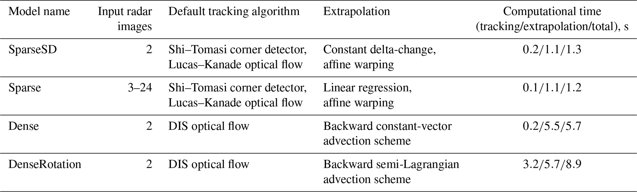
The benchmark models developed in this study consist of different combinations of algorithms for the two major steps of Lagrangian nowcasting frameworks, namely tracking and extrapolation (Austin and Bellon, 1974). Table 1 provides an overview of the models. The values of model parameters adopted in the benchmark experiment have been heuristically determined and not yet been subject to systematic optimization. However, the rainymotion library provides an opportunity to investigate how different optical flow model parameters can affect nowcasting results or how they can be tuned to represent, e.g., the typical range of advection speeds of real precipitation fields. For a description of parameters, please refer to Sect. S1 in the Supplement or the rainymotion library documentation (https://rainymotion.readthedocs.io/, last access: 28 March 2019).
Table 1Overview of the nowcasting models developed and their computational performance. Nowcasting experiments were carried out for 1 h lead time at a 5 min temporal resolution (12 resulting nowcast frames in total) using the RY radar data (spatial resolution of 1 km, grid size 900×900) and a standard office PC with an Intel® Core™ i7-2600 CPU (eight cores, 3.4 GHz).
2.1 The Sparse group
The central idea around this group of methods is to identify distinct features in a radar image that are suitable for tracking. In this context, a “feature” is defined as a distinct point (“corner”) with a sharp gradient of rainfall intensity. That approach is less arbitrary and scale dependent and thus more universal than classical approaches that track storm cells as contiguous objects (e.g., Wilson et al., 1998) because it eliminates the need to specify arbitrary and scale-dependent characteristics of “precipitation features” while the identification of corners depends only on the gradient sharpness in a cell's neighborhood. Inside this group, we developed two models that slightly differ with regard to both tracking and extrapolation.
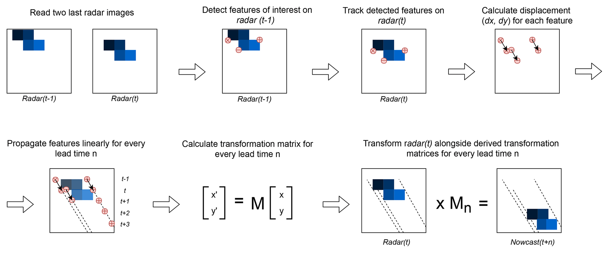
The first model (SparseSD, for Sparse Single Delta) uses only the two most recent radar images for identifying, tracking, and extrapolating features. Assuming that t denotes both the nowcast issue time and the time of the most recent radar image, the implementation can be summarized as follows.
-
Identify features in a radar image at time t−1 using the Shi–Tomasi corner detector (Shi and Tomasi, 1994). This detector determines the most prominent corners in the image based on the calculation of the corner quality measure (), where λ1 and λ2 are corresponding eigenvalues of the covariance matrix of derivatives over the neighborhood of 3×3 pixels) at each image pixel (see Sect. S1 for a detailed description of algorithm parameters).
-
Track these features at time t using the local Lucas–Kanade optical flow algorithm (Lucas and Kanade, 1981). This algorithm tries to identify the location of a feature we previously identified at time t−1 in the radar image at time t, based on solving a set of optical flow equations in the local feature neighborhood using the least-squares approach (see Sect. S1 for a detailed description of algorithm parameters).
-
Linearly extrapolate the features' motion in order to predict the features' locations at each lead time n.
-
Calculate the affine transformation matrix for each lead time n based on the locations of all identified features at time t and t+n using the least-squares approach (Schneider and Eberly, 2003). This matrix uniquely identifies the required transformation of the last observed radar image at time t so that the nowcast images at times provide the smallest possible difference between the locations of detected features at time t and the extrapolated features at times .
-
Extrapolate the radar image at time t by warping: for each lead time, the warping procedure uniquely transforms each pixel location of the radar image at time t to its future location in the nowcast radar images at times , using the affine transformation matrix. Remaining discontinuities in the predicted image are linearly interpolated in order to obtain nowcast intensities on a grid that corresponds to the radar image at time t (Wolberg, 1990).
To our knowledge, this study is the first to apply image warping directly as a simple and fast algorithm to represent advective motion of a precipitation field. In Sect. S2, you can find a simple synthetic example which shows the potential of the warping technique to replace an explicit advection formulation for temporal extrapolation.
For a visual representation of the SparseSD model, please refer to Fig. 1.
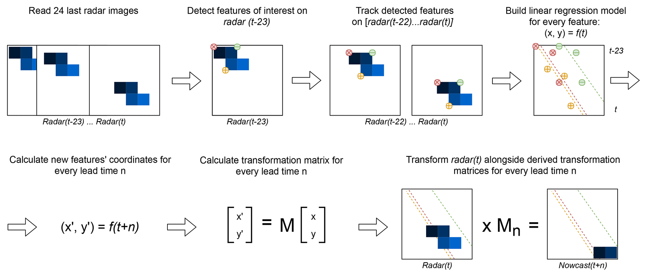
The second model (Sparse) uses the 24 most recent radar images, and we consider only features that are persistent over the whole period (of 24 time steps). The implementation can be summarized as follows.
-
Identify features on a radar image at time t−23 using the Shi–Tomasi corner detector (Shi and Tomasi, 1994).
-
Track these features in the radar images from t−22 to t using the local Lucas–Kanade optical flow algorithm (Lucas and Kanade, 1981).
-
Build linear regression models which independently parameterize changes in coordinates through time (from t−23 to t) for every successfully tracked feature.
-
Continue with steps 3–5 of SparseSD.
For a visual representation of the Sparse model, please refer to Fig. 2.
2.2 The Dense group
The Dense group of models uses, by default, the Dense Inverse Search algorithm (DIS) – a global optical flow algorithm proposed by Kroeger et al. (2016) – which allows us to explicitly estimate the velocity of each image pixel based on an analysis of two consecutive radar images. The DIS algorithm was selected as the default optical flow method for motion field retrieval because it showed, in our benchmark experiments, a higher accuracy and also a higher computational efficiency in comparison with other global optical flow algorithms such as DeepFlow (Weinzaepfel et al., 2013), and PCAFlow (Wulff and Black, 2015). We also tested the local Farnebäck algorithm (Farnebäck, 2003), which we modified by replacing zero velocities by interpolation and by smoothing the obtained velocity field based on a variational refinement procedure (Brox et al., 2004) (please refer to Sect. S5 for verification results of the corresponding benchmark experiment with various dense optical flow models). However, the rainymotion library provides the option to choose any of the optical flow methods specified above for precipitation nowcasting.
The two models in this group differ only with regard to the extrapolation (or advection) step. The first model (Dense) uses a constant-vector advection scheme (Bowler et al., 2004), while the second model (DenseRotation) uses a semi-Lagrangian advection scheme (Germann and Zawadzki, 2002). The main difference between both approaches is that a constant-vector scheme does not allow for the representation of rotational motion (Bowler et al., 2004); a semi-Lagrangian scheme allows for the representation of large-scale rotational movement while assuming the motion field itself to be persistent (Fig. 3).
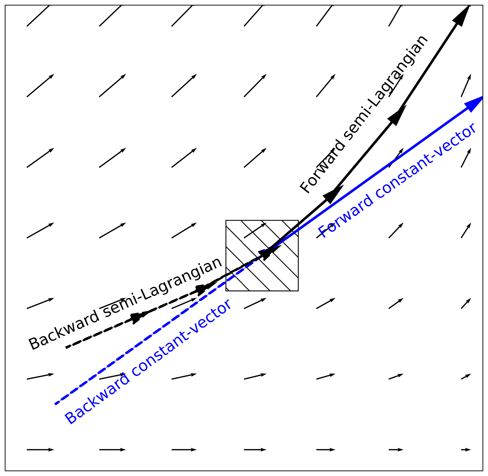
Figure 3Displacement vectors of four proposed advection schemes: forward or backward constant vector and forward or backward semi-Lagrangian.
There are two possible options of how both advection schemes may be implemented: forward in time (and downstream in space) or backward in time (and upstream in space) (Fig. 3). It is yet unclear which scheme can be considered as the most appropriate and universal solution for radar-based precipitation nowcasting, regarding the conservation of mass on the one hand and the attributed loss of power at small scales on the other hand (e.g., see discussion in Bowler et al., 2004; Germann and Zawadzki, 2002). Thus, we conducted a benchmark experiment with any possible combination of forward vs. backward and constant-vector vs. semi-Lagrangian advection. Based on the results (see Sect. S6), we use the backward scheme as the default option for both the Dense and DenseRotation models. However, the rainymotion library still provides the option to use the forward scheme, too.
Both the Dense and DenseRotation models utilize a linear interpolation procedure in order to interpolate advected rainfall intensities at their predicted locations to the native radar grid. The interpolation procedure “distributes” the value of a rain pixel to its neighborhood, as proposed in different modifications by Bowler et al. (2004), Liu et al. (2015), and Zahraei et al. (2012). The Dense group models' implementation can be summarized as follows.
-
Calculate a velocity field using the global DIS optical flow algorithm (Kroeger et al., 2016), based on the radar images at time t−1 and t.
-
Use a backward constant-vector (Bowler et al., 2004) or a backward semi-Lagrangian scheme (Germann and Zawadzki, 2002) to extrapolate (advect) each pixel according to the displacement (velocity) field, in one single step for each lead time t+n. For the semi-Lagrangian scheme, we update the velocity of the displaced pixels at each prediction time step n by linear interpolation of the velocity field to a pixel's location at that time step.
-
As a result of the advection step, we basically obtain an irregular point cloud that consists of the original radar pixels displaced from their original location. We use the intensity of each displaced pixel at its predicted location at time t+n in order to interpolate the intensity at each grid point of the original (native) radar grid (Liu et al., 2015; Zahraei et al., 2012), using the inverse distance weighting interpolation technique. It is important to note that we minimize numerical diffusion by first advecting each pixel over the target lead time before applying the interpolation procedure (as in the “interpolate once” approach proposed by Germann and Zawadzki, 2002). That way, we avoid rainfall features being smoothed in space by the effects of interpolation.
2.3 Persistence
The (trivial) benchmark model of Eulerian persistence assumes that for any lead time n, the precipitation field is the same as for time t. Despite its simplicity, it is quite a powerful model for very short lead times, and, at the same time, its verification performance is a good measure of temporal decorrelation for different events.
2.4 The rainymotion Python library
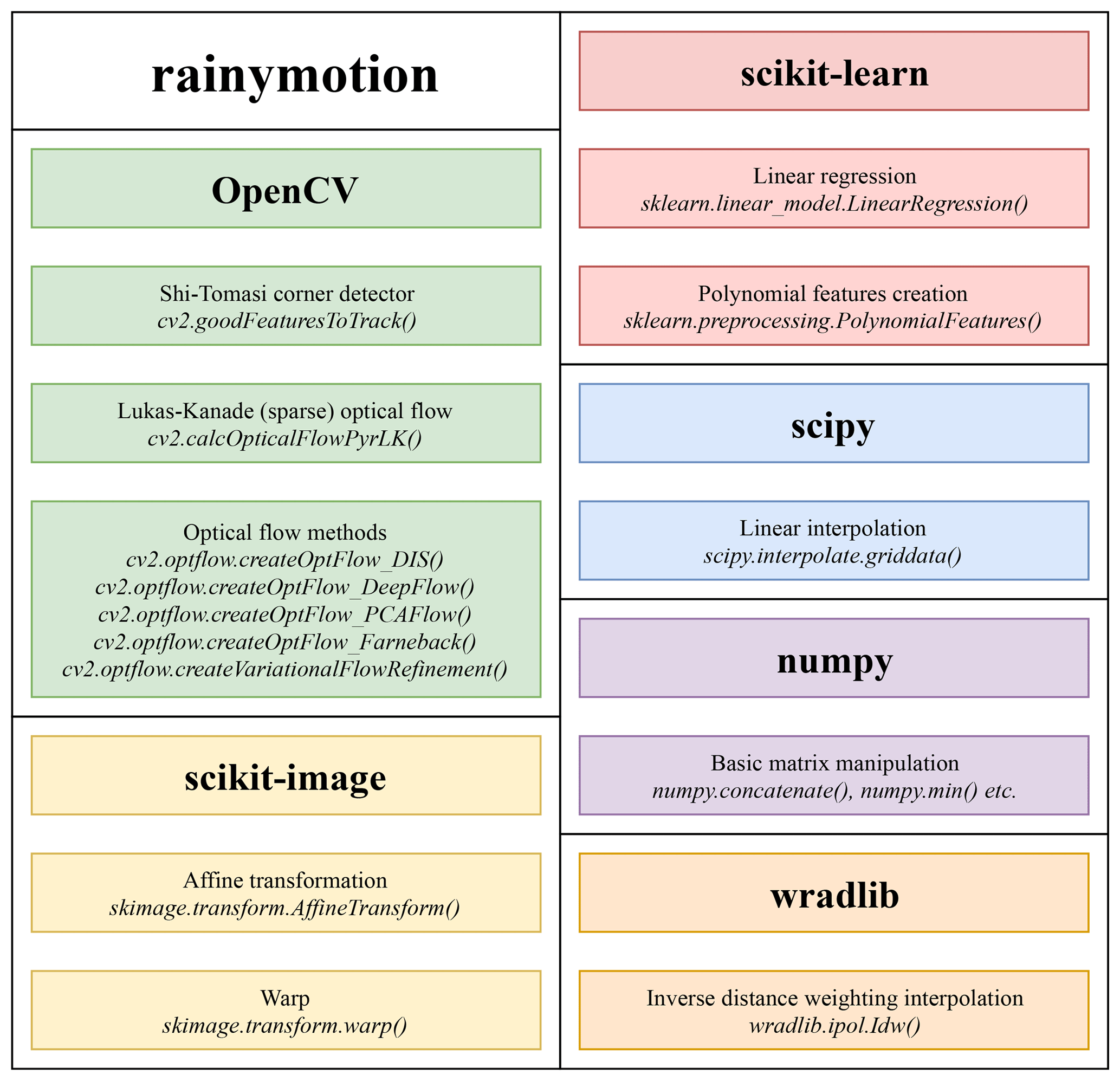
We have developed the rainymotion Python library to implement the above models. Since the rainymotion uses the standard format of numpy arrays for data manipulation, there is no restriction in using different data formats which can be read, transformed, and converted to numpy arrays using any tool from the set of available open software libraries for radar data manipulation (the list is available on https://openradarscience.org, last access: 28 March 2019). The source code is available in a Github repository (Ayzel et al., 2019) and has a documentation page (https://rainymotion.readthedocs.io, last access: 28 March 2019) which includes installation instructions, model description, and usage examples. The library code and accompanying documentation are freely distributed under the MIT software license which allows unrestricted use. The library is written in the Python 3 programming language (https://python.org, last access: 28 March 2019), and its core is entirely based on open-source software libraries (Fig. 4): ωradlib (Heistermann et al., 2013), OpenCV (Bradski and Kaehler, 2008), SciPy (Jones et al., 2018), NumPy (Oliphant, 2006), Scikit-learn (Pedregosa et al., 2011), and Scikit-image (Van der Walt et al., 2014). For generating figures we use the Matplotlib library (Hunter, 2007), and we use the Jupyter notebook (https://jupyter.org, last access: 28 March 2019) interactive development environment for code and documentation development and distribution. For managing the dependencies without any conflicts, we recommend to use the Anaconda Python distribution (https://anaconda.com, last access: 28 March 2019) and follow rainymotion installation instructions (https://rainymotion.readthedocs.io, last access: 28 March 2019).
2.5 Operational baseline (RADVOR)
The DWD operationally runs a stack of models for radar-based nowcasting and provides precipitation forecasts for a lead time up to 2 h. The operational QPN is based on the RADVOR module (Bartels et al., 2005; Rudolf et al., 2012). The tracking algorithm estimates the motion field from the latest sequential clutter-filtered radar images using a pattern recognition technique at different spatial resolutions (Winterrath and Rosenow, 2007; Winterrath et al., 2012). The focus of the tracking algorithm is on the meso-β scale (spatial extent: 25–250 km) to cover mainly large-scale precipitation patterns, but the meso-γ scale (spatial extension: 2.5–25 km) is also incorporated to allow the detection of smaller-scale convective structures. The resulting displacement field is interpolated to a regular grid, and a weighted averaging with previously derived displacement fields is implemented to guarantee a smooth displacement over time. The extrapolation of the most recent radar image according to the obtained velocity field is performed using a semi-Lagrangian approach. The described operational model is updated every 5 min and produces precipitation nowcasts at a temporal resolution of 5 min and a lead time of 2 h (RV product). In this study we used the RV product data as an operational baseline and did not re-implement the underlying algorithm itself.
3.1 Radar data and verification events
We use the so-called RY product of the DWD as input to our nowcasting models. The RY product represents a quality-controlled rainfall depth product that is a composite of the 17 operational Doppler radars maintained by the DWD. It has a spatial extent of 900 km×900 km and covers the whole area of Germany. Spatial and temporal resolution of the RY product is 1 km×1 km and 5 min, respectively. This composite product includes various procedures for correction and quality control (e.g., clutter removal). We used the ωradlib (Heistermann et al., 2013) software library for reading the DWD radar data.
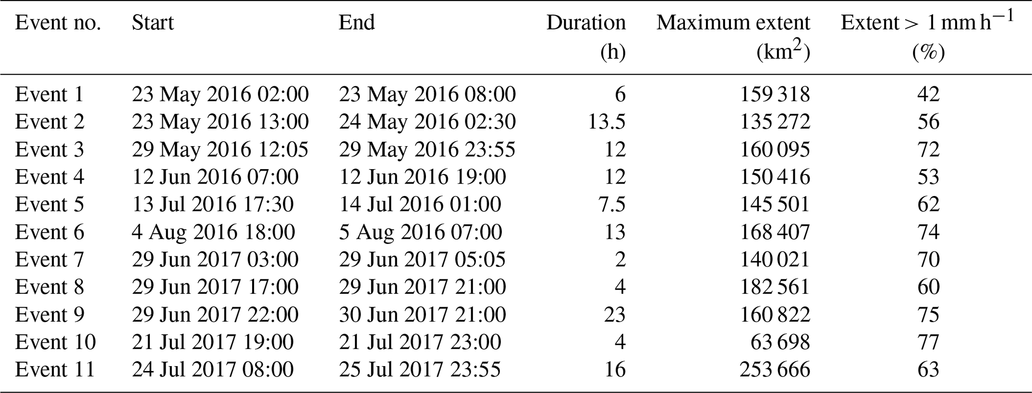
For the analysis, we selected 11 events during the summer periods of 2016 and 2017. These events are selected for covering a range of event characteristics with different rainfall intensity, spatial coverage, and duration. Table 2 shows the studied events. You can also find links to animations of event intensity dynamics in Sect. S3.
3.2 Verification metrics
For the verification we use two general categories of scores: continuous (based on the differences between nowcast and observed rainfall intensities) and categorical (based on standard contingency tables for calculating matches between Boolean values which reflect the exceedance of specific rainfall intensity thresholds). We use the mean absolute error (MAE) as a continuous score:
where nowi and obsi are nowcast and observed rainfall rate in the ith pixel of the corresponding radar image and n is the number of pixels. To compute the MAE, no pixels were excluded based on thresholds of nowcast or observed rainfall rate.
And we use the critical success index (CSI) as a categorical score:
where hits, false alarms, and misses are defined by the contingency table and the corresponding threshold value (for details see Sect. S4).
Following studies of Bowler et al. (2006) and Foresti et al. (2016), we have applied threshold rain rates of 0.125, 0.25, 0.5, 1, and 5 mm h−1 for calculating the CSI.
These two metrics inform us about the models' performance from the two perspectives: MAE captures errors in rainfall rate prediction (the less the better), and CSI captures model accuracy (the fraction of the forecast event that was correctly predicted; it does not distinguish between the sources of errors; the higher the better). You can find results represented in terms of additional categorical scores (false alarm rate, probability of detection, equitable threat score) in Sect. S4.
For each event, all models (Sparse, SparseSD, Dense, DenseRotation, Persistence) were used to compute nowcasts with lead times from 5 to 60 min (in 5 min steps). Operational nowcasts generated by the RADVOR system were provided by the DWD with the same temporal settings. An example of nowcasts for lead times 0, 5, 30, and 60 min is shown in Fig. 5.
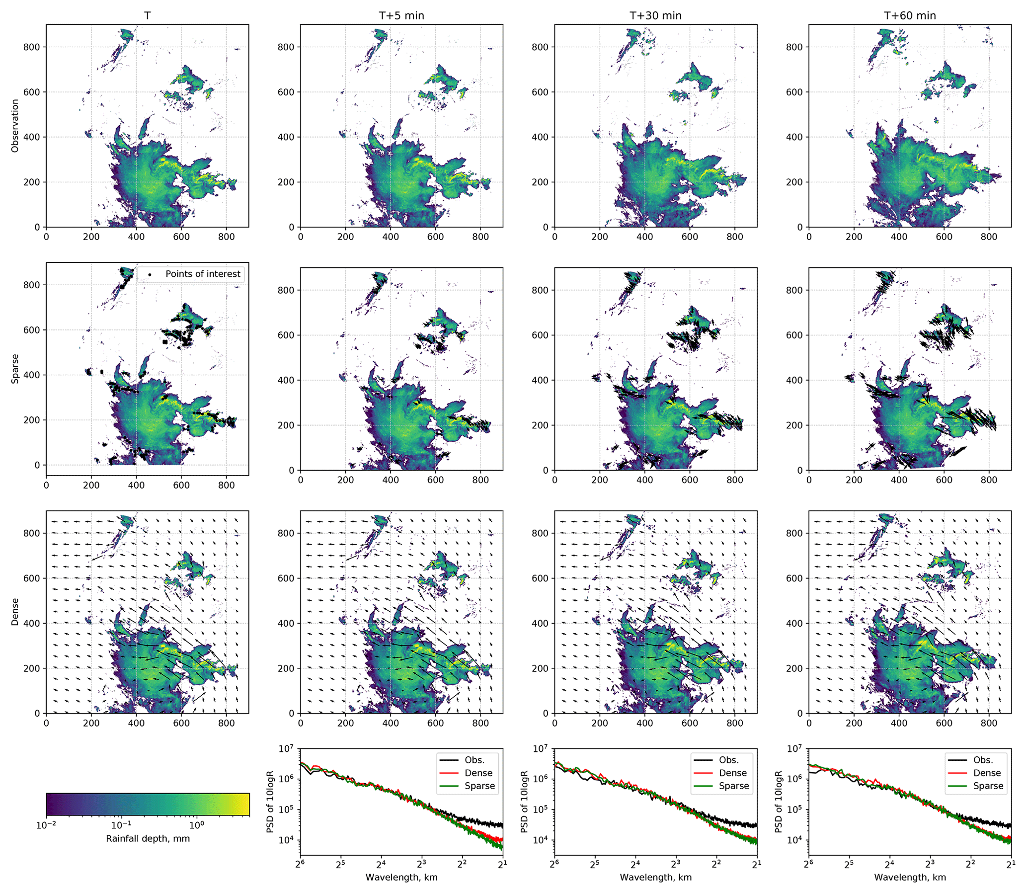
Figure 5Example of the nowcasting models output (SparseSD and Dense models) for the timestep, 29 May 2016, 19:15, and corresponding level of numerical diffusion (last row).
To investigate the effects of numerical diffusion, we calculated, for the same example, the power spectral density (PSD) of the nowcasts and the corresponding observations (bottom panels in Fig. 5) using Welch's method (Welch, 1967). Germann and Zawadzki (2002) showed that the most significant loss of power (lower PSD values) occurs at scales between 8 and 64 km. They did not analyze scales below 8 (23) km because their original grid resolution was 4 km. We extended the spectral analysis to consider scales as small as 21 km. Other than Germann and Zawadzki (2002), we could not observe any substantial loss of power between 8 and 64 km, yet Fig. 5 shows that both Dense and Sparse models consistently start to lose power at scales below 4 km. That loss does not depend much on the nowcast lead time, yet the Sparse group of models loses more power at a lead time of 5 min as compared to the Dense group. Still, these results rather confirm Germann and Zawadzki (2002): they show, as would be expected, that any loss of spectral power is most pronounced at the smallest scales and disappears at scales about 2–3 orders above the native grid resolution. For the investigated combination of data and models, this implies that our nowcasts will not be able to adequately represent rainfall features smaller than 4 km at lead times of up to 1 h.
Figure 6 shows the model performance (in terms of MAE) as a function of lead time. For each event, the Dense group of models is superior to the other ones. The RV product achieves an efficiency that is comparable to the Dense group. The SparseSD model outperforms the Sparse model for short lead times (up to 10–15 min) and vice versa for longer lead times. For some events (1–4, 6, 10, 11), the performance of the RV product appears to be particularly low in the first 10 min, compared to the other models. These events are characterized by particularly fast rainfall field movement.
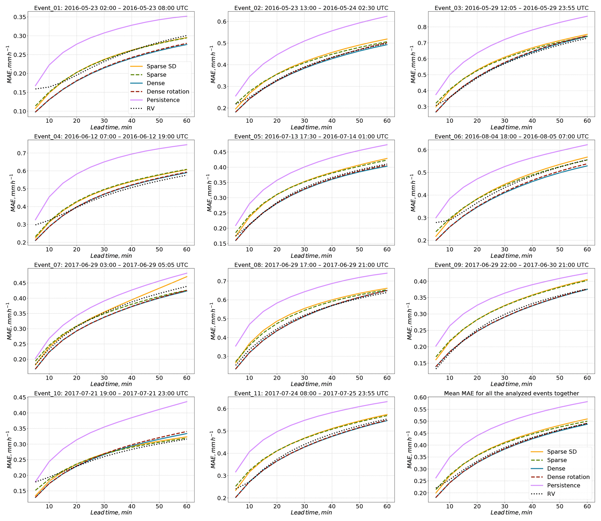
Figure 6Verification of the different optical flow based nowcasts in terms of MAE for 11 precipitation events over Germany.
Figure 7 has the same structure as Fig. 6 but shows the CSI with a threshold value of 1 mm h−1. For two events (7 and 10) the RV product achieves a comparable efficiency with the Dense group for lead times beyond 30 min. For the remaining events, the Dense group tends to outperform all other methods and the RV product achieves an average rank between models of the Sparse and Dense groups. For the Dense group of models, it appears that accounting for field rotation does not affect the results of the benchmark experiment much – the Dense and DenseRotation models perform very similarly, at least for the selected events and the analyzed lead times. The behavior of the Sparse group models is mostly consistent with the MAE.

Figure 7Verification of the different optical flow based nowcasts in terms of CSI for the threshold of 1 mm h−1 for 11 precipitation events over Germany.
Figure 8 shows the model performance using the CSI with a threshold value of 5 mm h−1. For the majority of events, the resulting ranking of models is the same as for the CSI with a threshold of 1 mm h−1. For events no. 2 and no. 3, the performance of the RV product relative to the Dense models is a little bit better, while for other events (e.g., no. 7), the Dense models outperform the RV product more clearly than for the CSI of 1 mm kh−1.
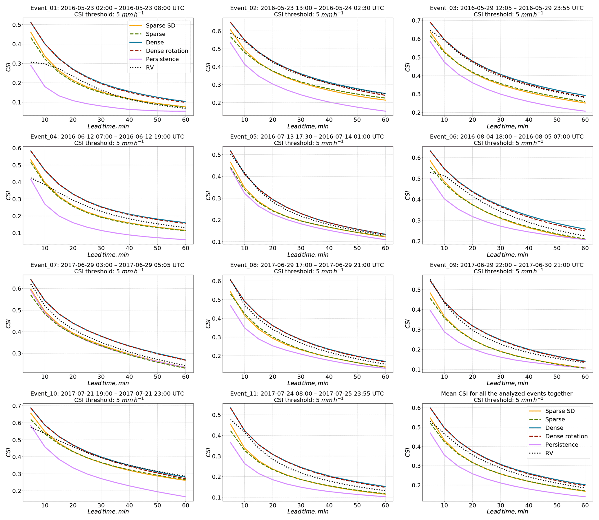
Figure 8Verification of the different optical flow based nowcasts in terms of CSI for the threshold of 5 mm h−1 for 11 precipitation events over Germany.
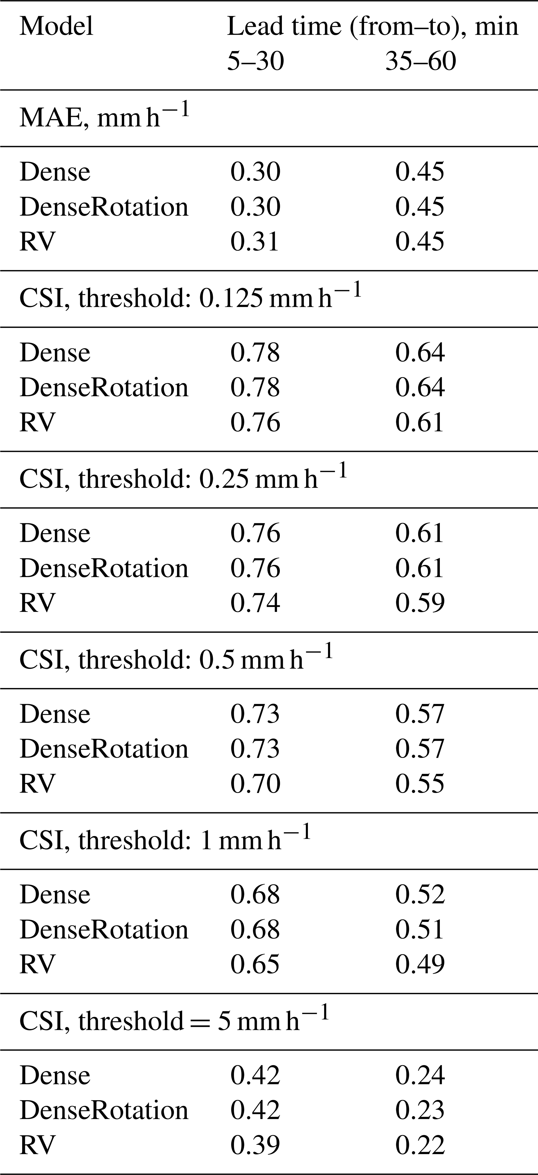
Table 3 summarizes the results of the Dense group models in comparison to the RV product for different verification metrics averaged over all the selected events and two lead time periods: 5–30 and 35–60 min. Results show that the Dense group always slightly outperforms the RV model in terms of CSI metric for both lead time periods and all analyzed rainfall intensity threshold used for CSI calculation. In terms of MAE, differences between model performances are less pronounced. For the CSI metric, the absolute differences between all models tend to be consistent with increasing rainfall thresholds.
You can find more figures illustrating the models' efficiency for different thresholds and lead times in Sect. S4.
5.1 Model comparison
All tested models show significant skill over the trivial Eulerian persistence over a lead time of at least 1 h. Yet a substantial loss of skill over lead time is present for all analyzed events, as expected. We have not disentangled the causes of that loss, but predictive uncertainty will always result from errors in both the representation of field motion and the total lack of representing precipitation formation, dynamics, and dissipation in a framework of Lagrangian persistence. Many studies specify a lead time of 30 min as a predictability limit for convective structures with fast dynamics of rainfall evolution (Foresti et al., 2016; Grecu and Krajewski, 2000; Thorndahl et al., 2017; Wilson et al., 1998; Zahraei et al., 2012). Our study confirms these findings.
For the majority of analyzed events, there is a clear pattern that the Dense group of optical flow models outperforms the operational RV nowcast product. For the analyzed events and lead times, the differences between the Dense and the DenseRotation models (or, in other words, between constant-vector and semi-Lagrangian schemes) are negligible. The absolute difference in performance between the Dense group models and the RV product appears to be independent of rainfall intensity threshold and lead time (Table 3), which implies that the relative advance of the Dense group models over the RV product increases both with lead time and rainfall intensity threshold. A gain in performance for longer lead times by taking into account more time steps from the past can be observed when comparing the SparseSD model (looks back 5 min in time) against the Sparse model (looks back 2 h in time).
Despite their skill over Eulerian persistence, the Sparse group models are significantly outperformed by the Dense group models for all the analyzed events and lead times. The reason for this behavior still remains unclear. It could, in general, be a combination of errors introduced in corner tracking and extrapolation as well as image warping as a surrogate for formal advection. While the systematic identification of error sources will be subject to future studies, we suspect that the local features (corners) identified by the Shi–Tomasi corner detector might not be representative of the overall motion of the precipitation field: the detection focuses on features with high intensities and gradients, the motion of which might not represent the dominant meso-γ-scale motion patterns.
There are a couple of possible directions for enhancing the performance for longer lead times using the Dense group of models. A first is to use a weighted average of velocity fields derived from radar images three (or more) steps back in time (as done in RADVOR to compute the RV product). A second option is to calculate separate velocity fields for low-and high-intensity subregions of the rain field and advect these subregions separately (as proposed in Golding, 1998) or find an optimal weighting procedure. A third approach could be to optimize the use of various optical flow constraints in order to improve the performance for longer lead times, as proposed in Germann and Zawadzki (2002), Bowler et al. (2004), or Mecklenburg et al. (2000). The flexibility of the rainymotion software library allows users to incorporate such algorithms for benchmarking any hypothesis, and, for example, implement different models or parameterizations for different lead times. Bowler et al. (2004) also showed a significant performance increase for longer lead times by using NWP model winds for the advection step. However, Winterrath and Rosenow (2007) did not obtain any improvement compared to RADVOR for longer lead times by incorporating NWP model winds into the nowcasting procedure.
5.2 Advection schemes properties and effectiveness
Within the Dense group of models, we could not find any significant difference between the performance and PSD of the constant-vector (Dense model) and the semi-Lagrangian scheme (DenseRotation). That confirms findings presented by Germann and Zawadzki (2002), who found that the constant vector and the modified semi-Lagrangian schemes have very similar power spectra, presumably since they share the same interpolation procedure. The theoretical superiority of the semi-Lagrangian scheme might, however, materialize for other events with substantial, though persistent rotational motion. A more comprehensive analysis should thus be undertaken in future studies.
Interpolation is included in both the post-processing of image warping (Sparse models) and in the computation of gridded nowcasts as part of the Dense models. In general, such interpolation steps can lead to numerical diffusion and thus to the degradation or loss of small-scale features (Germann and Zawadzki, 2002). Yet we were mostly able to contain such adverse effects for both the Sparse and the Dense group of models by carrying out only one interpolation step for any forecast at a specific lead time. We showed that numerical diffusion was negligible for lead times of up to 1 h for any model; however, as has been shown in Germann and Zawadzki (2002), for longer lead times these effects can be significant, depending on the implemented extrapolation technique.
5.3 Computational performance
Computational performance might be an important criterion for end users aiming at frequent update cycles. We ran our nowcasting models on a standard office PC with an Intel® Core™ i7-2600 CPU (eight cores, 3.4 GHz), and on a standard laptop with an Intel® Core™ i5-7300HQ CPU (four cores, 2.5 GHz). The average time for generating one nowcast for 1 h lead time (at 5 min resolution) is 1.5–3 s for the Sparse group and 6–12 s for the Dense group. The Dense group is computationally more expensive due to interpolation operations implemented for large grids (900×900 pixels). There is also potential for increasing the computational performance of the interpolation.
Optical flow is a technique for deriving a velocity field from consecutive images. It is widely used in image analysis and has become increasingly popular in meteorological applications over the past 20 years. In our study, we examined the performance of optical-flow-based models for radar-based precipitation nowcasting, as implemented in the open-source rainymotion library, for a wide range of rainfall events using radar data provided by the DWD.
Our benchmark experiments, including an operational baseline model (the RV product provided by the DWD), show a firm basis for using optical flow in radar-based precipitation nowcasting studies. For the majority of the analyzed events, models from the Dense group outperform the operational baseline. The Sparse group of models showed significant skill, yet they generally performed more poorly than both the Dense group and the RV product. We should, however, not prematurely discard the group of Sparse models before we have not gained a better understanding of error sources with regard to the tracking, extrapolation, and warping steps. Combining the warping procedure for the extrapolation step with the Dense optical flow procedure for the tracking step (i.e., to advect corners based on a “Dense” velocity field obtained by implementing one of the dense optical flow techniques) might also be considered. This opens the way for merging two different model development branches in the future releases of the rainymotion library.
There is a clear and rapid model performance loss over lead time for events with high rainfall intensities. This issue continues to be unresolved by standard nowcasting approaches, but some improvement in this field may be achieved by using strategies such as merging with NWP results and stochastic modeling of rainfall field evolution. Admittedly, deterministic nowcasts in a Lagrangian framework account neither for precipitation intensity dynamics nor for the uncertainties in representing precipitation field motion. At least for the latter, the rainymotion library provides ample opportunities to experiment with forecast ensembles, based on various tracking and extrapolation techniques. Furthermore, we suppose that using new data-driven models based on machine and deep learning may increase the performance by utilizing and structuring common patterns in the massive archives of radar data.
We do not claim that the developed models will compete with well-established and excessively tuned operational models for radar-based precipitation nowcasting. Yet we hope our models may serve as an essential tool for providing a fast, free, and open-source solution that can serve as a benchmark for further model development and hypothesis testing – a benchmark that is far more advanced than the conventional benchmark of Eulerian persistence.
Recent studies show that open-source community-driven software advances the field of weather radar science (Heistermann et al., 2015a, b). Just a few months ago, the pySTEPS (https://pysteps.github.io, last access: 28 March 2019) initiative was introduced “to develop and maintain an easy to use, modular, free and open-source python framework for short-term ensemble prediction systems”. As another piece of evidence of the dynamic evolution of QPN research over the recent years, these developments could pave the way for future synergies between the pySTEPS and rainymotion projects – towards the availability of open, reproducible, and skillful methods in quantitative precipitation nowcasting.
The rainymotion library is free and open-source. It is distributed under the MIT software license, which allows unrestricted use. The source code is provided through a GitHub repository (Ayzel et al., 2019), the snapshot of the rainymotion v0.1 is also available on Zenodo: https://doi.org/10.5281/zenodo.2561583 (Ayzel, 2019), and the documentation is available on a website (https://rainymotion.readthedocs.io, last access: 28 March 2019). The DWD provided the sample data of the RY product, and they are distributed with the rainymotion repository to provide a real-case and reproducible example of precipitation nowcasting.
The supplement related to this article is available online at: https://doi.org/10.5194/gmd-12-1387-2019-supplement.
GA performed the benchmark experiments, analyzed the data, and wrote the paper. MH coordinated and supervised the work, analyzed the data, and wrote the paper. TW assisted in the data retrieval and analysis and shared her expertise in DWD radar products.
The authors declare that they have no conflict of interest.
Georgy Ayzel was financially supported by Geo.X, the Research Network for Geosciences in Berlin and Potsdam. The authors thank Loris Foresti, Seppo Pulkkinen, and Remko Uijlenhoet for their constructive comments and suggestions that helped to improve the paper. We acknowledge the support of Deutsche Forschungsgemeinschaft (German Research Foundation) and the Open Access Publication Fund of Potsdam University.
This paper was edited by Axel Lauer and reviewed by Seppo Pulkkinen, Remko Uijlenhoet, and Loris Foresti.
Austin, G. L. and Bellon, A.: The use of digital weather radar records for short-term precipitation forecasting, Q. J. Roy. Meteor. Soc., 100, 658–664, https://doi.org/10.1002/qj.49710042612, 1974. a, b
Ayzel, G.: hydrogo/rainymotion: rainymotion v0.1, Version v0.1, Zenodo, https://doi.org/10.5281/zenodo.2561583, 2019. a
Ayzel, G., Heistermann, M., and Winterrath, T.: rainymotion: python library for radar-based precipitation nowcasting based on optical flow techniques, available at: https://github.com/hydrogo/rainymotion (last access: 28 March 2019), 2019. a, b, c, d
Bauer, P., Thorpe, A., and Brunet, G.: The quiet revolution of numerical weather prediction, Nature, 525, 47–55, https://doi.org/10.1038/nature14956, 2015. a
Bellerby, T. J.: High-resolution 2-D cloud-top advection from geostationary satellite imagery, IEEE T. Geosci. Remote, 44, 3639–3648, https://doi.org/10.1109/TGRS.2006.881117, 2006. a
Berenguer, M., Sempere-Torres, D., and Pegram, G. G. S.: SBMcast – An ensemble nowcasting technique to assess the uncertainty in rainfall forecasts by Lagrangian extrapolation, J. Hydrol., 404, 226–240, https://doi.org/10.1016/j.jhydrol.2011.04.033, 2011. a, b
Berenguer, M., Surcel, M., Zawadzki, I., Xue, M., Kong, F., Berenguer, M., Surcel, M., Zawadzki, I., Xue, M., and Kong, F.: The Diurnal Cycle of Precipitation from Continental Radar Mosaics and Numerical Weather Prediction Models. Part II: Intercomparison among Numerical Models and with Nowcasting, Mon. Weather Rev., 140, 2689–2705, https://doi.org/10.1175/MWR-D-11-00181.1, 2012. a
Bowler, N. E., Pierce, C. E., and Seed, A.: Development of a precipitation nowcasting algorithm based upon optical flow techniques, J. Hydrol., 288, 74–91, https://doi.org/10.1016/j.jhydrol.2003.11.011, 2004. a, b, c, d, e, f, g, h, i
Bowler, N. E., Pierce, C. E., and Seed, A. W.: STEPS: A probabilistic precipitation forecasting scheme which merges an extrapolation nowcast with downscaled NWP, Q. J. Roy. Meteor. Soc., 132, 2127–2155, https://doi.org/10.1256/qj.04.100, 2006. a, b, c
Bradski, G. and Kaehler, A.: Learning OpenCV: Computer vision with the OpenCV library, O'Reilly Media, Inc., 2008. a
Brox, T., Bruhn, A., Papenberg, N., and Weickert, J.: High accuracy optical flow estimation based on a theory for warping, in: Computer Vision – ECCV 2004. Lecture Notes in ComputerScience, edited by: Pajdla, T. and Matas, J., Springer, Berlin, 3024, 25–36, 2004. a, b
Bruhn, A., Weickert, J., Feddern, C., Kohlberger, T., and Schnörr, C.: Variational optical flow computation in real time, IEEE T. Image Process., 14, 608–615, https://doi.org/10.1109/TIP.2005.846018, 2005a. a
Bruhn, A., Weickert, J., and Schnörr, C.: Lucas/Kanade meets Horn/Schunck: Combining local and global optic flow methods, Int. J. Comput. Vision, 61, 211–231, 2005b. a
Cheung, P. and Yeung, H. Y.: Application of optical-flow technique to significant convection nowcast for terminal areas in Hong Kong, in: The 3rd WMO International Symposium on Nowcasting and Very Short-Range Forecasting (WSN12), Rio de Janeiro, Brazil, 6–10 August 2012, Reprint 1025, 10 pp., available at: http://www.hko.gov.hk/publica/reprint/r1025.pdf (last access: 28 March 2019), 2012. a, b, c
Farnebäck, G.: Two-frame motion estimation based on polynomial expansion, in: Image Analysis, SCIA 2003, Lecture Notes in Computer Science, edited by: Bigun, J. and Gustavsson, T., Springer, Berlin, Heidelberg, 2749, 363–370, https://doi.org/10.1007/3-540-45103-x_50, 2003. a
Foresti, L., Reyniers, M., Seed, A., and Delobbe, L.: Development and verification of a real-time stochastic precipitation nowcasting system for urban hydrology in Belgium, Hydrol. Earth Syst. Sci., 20, 505–527, https://doi.org/10.5194/hess-20-505-2016, 2016. a, b, c, d, e
Germann, U. and Zawadzki, I.: Scale-Dependence of the Predictability of Precipitation from Continental Radar Images. Part I: Description of the Methodology, Mon. Weather Rev., 130, 2859–2873, https://doi.org/10.1175/1520-0493(2002)130<2859:SDOTPO>2.0.CO;2, 2002. a, b, c, d, e, f, g, h, i, j, k, l, m, n, o, p
Golding, B. W.: Nimrod: A system for generating automated very short range forecasts, Meteorol. Appl., 5, 1–16, https://doi.org/10.1017/S1350482798000577, 1998. a
Grecu, M. and Krajewski, W. F.: A large-sample investigation of statistical procedures for radar-based short-term quantitative precipitation forecasting, J. Hydrol., 239, 69–84, https://doi.org/10.1016/S0022-1694(00)00360-7, 2000. a, b, c
Heistermann, M., Jacobi, S., and Pfaff, T.: Technical Note: An open source library for processing weather radar data (wradlib), Hydrol. Earth Syst. Sci., 17, 863–871, https://doi.org/10.5194/hess-17-863-2013, 2013. a, b
Heistermann, M., Collis, S., Dixon, M. J., Giangrande, S., Helmus, J. J., Kelley, B., Koistinen, J., Michelson, D. B., Peura, M., Pfaff, T., and Wolff, D. B.: The emergence of open-source software for the weather radar community, B. Am. Meteorol. Soc., 96, 117–128, https://doi.org/10.1175/BAMS-D-13-00240.1, 2015a. a
Heistermann, M., Collis, S., Dixon, M. J., Helmus, J. J., Henja, A., Michelson, D. B., and Pfaff, T.: An open virtual machine for cross-platform weather radar science, B. Am. Meteorol. Soc., 96, 1641–1645, https://doi.org/10.1175/BAMS-D-14-00220.1, 2015b. a
Horn, B. K. and Schunck, B. G.: Determining optical flow, Artif. Intell., 17, 185–203, 1981. a, b
Hunter, J. D.: Matplotlib: A 2D graphics environment, Comput. Sci. Eng., 9, 90–95, 2007. a
Jensen, D. G., Petersen, C., and Rasmussen, M. R.: Assimilation of radar-based nowcast into a HIRLAM NWP model, Meteorol. Appl., 22, 485–494, https://doi.org/10.1002/met.1479, 2015. a
Jones, E., Oliphant, T., and Peterson, P.: SciPy: open source scientific tools for Python, available at: https://scipy.org/, last access: 29 June 2018. a
Kroeger, T., Timofte, R., Dai, D., and Van Gool, L.: Fast optical flow using dense inverse search, in: Computer Vision – ECCV 2016. ECCV 2016. Lecture Notes in Computer Science, edited by: Leibe, B., Matas, J., Sebe, N., and Welling, M., Springer, Cham, 9908, 471–488, https://doi.org/10.1007/978-3-319-46493-0_29, 2016. a, b, c
Lin, C., Vasić, S., Kilambi, A., Turner, B., and Zawadzki, I.: Precipitation forecast skill of numerical weather prediction models and radar nowcasts, Geophys. Res. Lett., 32, L14801, https://doi.org/10.1029/2005GL023451, 2005. a
Liu, Y., Xi, D. G., Li, Z. L., and Hong, Y.: A new methodology for pixel-quantitative precipitation nowcasting using a pyramid Lucas Kanade optical flow approach, J. Hydrol., 529, 354–364, https://doi.org/10.1016/j.jhydrol.2015.07.042, 2015. a, b, c, d, e, f, g
Lucas, B. D. and Kanade, T.: An iterative image Registration Technique with an Application to Stereo Vision, in: Proceedings DARPA Image Understanding Workshop, Vancouver, BC, Canada, 24–28 August 1981, 674–679, 1981 a, b, c, d
Mecklenburg, S., Joss, J., and Schmid, W.: Improving the nowcasting of precipitation in an Alpine region with an enhanced radar echo tracking algorithm, J. Hydrol., 239, 46–68, https://doi.org/10.1016/S0022-1694(00)00352-8, 2000. a
Mueller, C. M., Axen, T. S., Oberts, R. R., Ilson, J. W., Etancourt, T. B., Ettling, S. D., and Ien, N. O.: NCAR Auto-Nowcast System, Weather Forecast., 18, 545–561, https://doi.org/10.1175/1520-0434(2003)018<0545:NAS>2.0.CO;2, 2003. a
Oliphant, T. E.: A guide to NumPy, vol. 1, Trelgol Publishing, USA, 2006. a
Pedregosa, F., Varoquaux, G., Gramfort, A., Michel, V., Thirion, B., Grisel, O., Blondel, M., Prettenhofer, P., Weiss, R., Dubourg, V., Vanderplas, J., Passos, A., and Cournapeau D.: Scikit-learn: Machine learning in Python, J. Mach. Learn. Res., 12, 2825–2830, 2011. a
Reyniers, M.: Quantitative precipitation forecasts based on radar observations: Principles, algorithms and operational systems, Institut Royal Météorologique de Belgique, available at: https://www.meteo.be/meteo/download/fr/3040165/pdf/rmi_scpub-1261.pdf (last access: 28 March 2019), 2008. a
Ruzanski, E., Chandrasekar, V., and Wang, Y.: The CASA nowcasting system, J. Atmos. Ocean. Tech., 28, 640–655, https://doi.org/10.1175/2011JTECHA1496.1, 2011. a
Schneider, P. J. and Eberly, D. H.: Geometric tools for computer graphics, Boston, available at: https://www.sciencedirect.com/science/book/9781558605947 (last access: 28 March 2019), 2003. a
Shi, J. and Tomasi, C.: Good features to track, in: 1994 Proceedings of IEEE Conference on Computer Vision and Pattern Recognition, Seattle, WA, USA, USA, 21–23 June 1994, IEEE, 593–600, https://doi.org/10.1109/CVPR.1994.323794, 1994. a, b
Thorndahl, S., Einfalt, T., Willems, P., Nielsen, J. E., ten Veldhuis, M.-C., Arnbjerg-Nielsen, K., Rasmussen, M. R., and Molnar, P.: Weather radar rainfall data in urban hydrology, Hydrol. Earth Syst. Sci., 21, 1359–1380, https://doi.org/10.5194/hess-21-1359-2017, 2017. a
Van der Walt, S., Schönberger, J. L., Nunez-Iglesias, J., Boulogne, F., Warner, J. D., Yager, N., Gouillart, E., and Yu, T.: scikit-image: image processing in Python, PeerJ, 2, e453, https://doi.org/10.7717/peerj.453, 2014. a
Weinzaepfel, P., Revaud, J., Harchaoui, Z., and Schmid, C.: DeepFlow: Large Displacement Optical Flow with Deep Matching, in: 2013 IEEE International Conference on Computer Vision, Sydney, NSW, Australia, 1–8 December 2013, IEEE, 1385–1392, https://doi.org/10.1109/ICCV.2013.175, 2013. a
Welch, P.: The use of fast Fourier transform for the estimation of power spectra: a method based on time averaging over short, modified periodograms, IEEE T. Acoust. Speech, 15, 70–73, 1967. a
Wilson, J. W., Crook, N. A., Mueller, C. K., Sun, J., and Dixon, M.: Nowcasting Thunderstorms: A Status Report, B. Am. Meteorol. Soc., 79, 2079–2099, https://doi.org/10.1175/1520-0477(1998)079<2079:NTASR>2.0.CO;2, 1998. a, b
Winterrath, T. and Rosenow, W.: A new module for the tracking of radar-derived precipitation with model-derived winds, Adv. Geosci., 10, 77–83, https://doi.org/10.5194/adgeo-10-77-2007, 2007. a
Winterrath, T., Rosenow, W., and Weigl, E.: On the DWD quantitative precipitation analysis and nowcasting system for real-time application in German flood risk management, in: Weather Radar and Hydrology (Proceedings of a symposium held in Exeter, UK, April 2011), IAHS Publ. 351, 323–329, available at: https://www.dwd.de/DE/leistungen/radolan/radolan_info/Winterrath_German_flood_risk_management_pdf.pdf? blob=publicationFile&v=4 (last access: 28 March 2019), 2012. a
Wolberg, G.: Digital Image Warping, IEEE Computer Society Press, Los Alamitos, CA, USA, 1990. a
Wong, W. K., Yeung, L. H. Y., Wang, Y. C., and Chen, M.: Towards the blending of NWP with nowcast – Operation experience in B08FDP, WMO Symposium on Nowcasting, 30 August–4 September 2009, Whistler, B.C., Canada, available at: http://my.hko.gov.hk/publica/reprint/r844.pdf (last access: 28 March 2019), 2009. a
Woo, W.-C. and Wong, W.-K.: Operational Application of Optical Flow Techniques to Radar-Based Rainfall Nowcasting, Atmosphere, 8, 48, https://doi.org/10.3390/atmos8030048, 2017. a, b, c, d
Wulff, J. and Black, M. J.: Efficient Sparse-to-Dense Optical Flow Estimation Using a Learned Basis and Layers, in: IEEE Conf. on Computer Vision and Pattern Recognition (CVPR 2015), Boston, MA, USA, 7–12 June 2015, 120–130, 2015. a
Yeung, L. H. Y., Wong, W. K., Chan, P. K. Y., Lai, E. S. T., Yeung, L. H. Y., Wong, W. K., Chan, P. K. Y., and Lai, E. S. T.: Applications of the Hong Kong Observatory nowcasting system SWIRLS-2 in support of the 2008 Beijing Olympic Games, in: WMO Symposium on Nowcasting, 30 August–4 September 2009, Whistler, B.C., Canada, available at: http://my.hko.gov.hk/publica/reprint/r843.pdf (last access: 28 March 2019), 2009. a
Zahraei, A., lin Hsu, K., Sorooshian, S., Gourley, J. J., Lakshmanan, V., Hong, Y., and Bellerby, T.: Quantitative Precipitation Nowcasting: A Lagrangian Pixel-Based Approach, Atmos. Res., 118, 418–434, https://doi.org/10.1016/j.atmosres.2012.07.001, 2012. a, b, c, d, e
Zahraei, A., lin Hsu, K., Sorooshian, S., Gourley, J. J., Hong, Y., and Behrangi, A.: Short-term quantitative precipitation forecasting using an object-based approach, J. Hydrol., 483, 1–15, https://doi.org/10.1016/j.jhydrol.2012.09.052, 2013. a