the Creative Commons Attribution 4.0 License.
the Creative Commons Attribution 4.0 License.
 | 26 Apr 2019
A statistical and process-oriented evaluation of cloud radiative effects in high-resolution global models
Abhay Devasthale
Torben Koenigk
Klaus Wyser
Malcolm Roberts
Christopher Roberts
Katja Lohmann
This study evaluates the impact of atmospheric horizontal resolution on the representation of cloud radiative effects (CREs) in an ensemble of global climate model simulations following the protocols of the High Resolution Model Intercomparison Project (HighResMIP). We compare results from four European modelling centres, each of which provides data from “standard”- and “high”-resolution model configurations. Simulated radiative fluxes are compared with observation-based estimates derived from the Clouds and Earth's Radiant Energy System (CERES) dataset. Model CRE biases are evaluated using both conventional statistics (e.g. time and spatial averages) and after conditioning on the phase of two modes of internal climate variability, namely the El Niño–Southern Oscillation (ENSO) and the North Atlantic Oscillation (NAO). Simulated top-of-atmosphere (TOA) and surface CREs show large biases over the polar regions, particularly over regions where seasonal sea-ice variability is strongest. Increasing atmospheric resolution does not significantly improve these biases. The spatial structure of the cloud radiative response to ENSO and NAO variability is simulated reasonably well by all model configurations considered in this study. However, it is difficult to identify a systematic impact of atmospheric resolution on the associated CRE errors. Mean absolute CRE errors conditioned on the ENSO phase are relatively large (5–10 W m−2) and show differences between models. We suggest this is a consequence of differences in the parameterization of SW radiative transfer and the treatment of cloud optical properties rather than a result of differences in resolution. In contrast, mean absolute CRE errors conditioned on the NAO phase are generally smaller (0–2 W m−2) and more similar across models. Although the regional details of CRE biases show some sensitivity to atmospheric resolution within a particular model, it is difficult to identify patterns that hold across all models. This apparent insensitivity to increased atmospheric horizontal resolution indicates that physical parameterizations play a dominant role in determining the behaviour of cloud–radiation feedbacks. However, we note that these results are obtained from atmosphere-only simulations and the impact of changes in atmospheric resolution may be different in the presence of coupled climate feedbacks.
- Article
(36828 KB) - Full-text XML
- BibTeX
- EndNote


Clouds cover about 70 % of the Earth's area and have multiple effects on climate (Karlsson and Devasthale, 2018; Stubenrauch et al., 2013). They regulate the Earth's radiation budget by modulating the incoming solar radiation as well as the outgoing longwave radiation (Stephens et al., 2018). Cloud processes occur from micrometre (e.g. condensation or freezing) to kilometre scales (e.g. convective systems). Clouds also have a strong dynamic character and vary substantially in space and time in the atmosphere (Steiner et al., 2018). Given the complexity of cloud–climate interactions, cloud processes are heavily parameterized in climate models. Considering their tight coupling to the radiation budget, they are one of the key components of the Earth system that need to be evaluated in the global climate models. Evaluating clouds requires a two-pronged approach, wherein both statistical and process-oriented comparisons with observations are needed. In the former, the absolute biases in cloud properties and cloud radiative effects by statistical comparisons of mean fields are carried out, whereas the degree with which a certain cloud process is simulated by climate models is assessed in the latter.
Atmospheric processes, especially those related to cloud–climate interactions, are sensitive to the spatial resolution of climate models. For example, increasing the spatial resolution in models is shown to be crucial to accurately reproduce the large-scale features such as the El Niño–Southern Oscillation (Shaevitz et al., 2014; Masson et al., 2012), Intertropical Convergence Zone (ITCZ) (Doi et al., 2012), jet streams (Lu et al., 2015; Sakaguchi et al., 2015) and storm tracks (Hodges et al., 2011). Improvements are also seen in the simulation of synoptic-scale phenomena such as tropical cyclones (Murakami et al., 2015; Walsh et al., 2015; Shaevitz et al., 2014) and polar lows (Zappa et al., 2014). A detailed overview of the improvements in the key climate processes is addressed in Haarsma et al. (2016). In light of these studies, the EU-funded PRIMAVERA (PRocess-based climate sIMulation: AdVances in high resolution modelling and European climate Risk Assessment) project (https://www.primavera-h2020.eu/, last access: 9 February 2019) aims at improving our understanding of the role that an increased spatial resolution plays in simulating climate processes and their feedbacks.
Here, in the context of this PRIMAVERA project, the surface and top-of-the-atmosphere cloud radiative effects (CREs) are analyzed in global climate models from four European modelling centres, each with varying spatial resolutions. The observed flux estimates from NASA's CERES-EBAF (Clouds and the Earth's Radiant Energy System-Energy Balanced And Filled) instrument is used for the evaluation. CERES provides the longest, continuous space-based global observations of cloud forcings. Evaluating climate models provides a positive feedback loop, wherein as the climate models improve, in part due to better observations; the requirements on observations have also increased (Flato et al., 2013; Ferraro et al., 2015; Webb et al., 2017). Particularly, the last decade has seen an exponential increase and maturity in observations and, as a result, has provided greater insights into model deficiencies and limitations (Reichler and Kim, 2001; Tian et al., 2013; Teixeira et al., 2014; Baker and Taylor, 2016).
In the present study, we carry out evaluations using both approaches, i.e. the statistical and process-oriented comparisons. For the latter, we focus on two major modes of natural variability, namely ENSO and North Atlantic Oscillation (NAO), that govern the atmospheric variability in the tropical Pacific and North Atlantic oceans and the surrounding continents. First, the typical cloud radiative response to ENSO and NAO is investigated, and then we test how well this response is simulated by climate models. Cloud radiative response is defined as the change in cloud radiative effects observed during the positive and negative phases of ENSO and NAO compared to climatology. We further investigated if high spatial resolution adds value while capturing the cloud radiative response during these two major modes of natural variability.
2.1 Models participated in the PRIMAVERA project
The shortwave (SW), longwave (LW) and combined cloud radiative effects (CREs) are evaluated in the High Resolution Model Intercomparison Project (HighResMIP; Haarsma et al., 2016) models with varying resolutions that participated in the PRIMAVERA project. A brief description of these models used in this study is provided in the table below. The atmosphere-only simulations are forced by sea surface temperature (SST) and sea ice concentrations from the Hadley Centre Sea Ice and Sea Surface Temperature data set version 2.2 (HadISST2.2; Kennedy et al., 2017). The HadGEM3 model is the only model that is run at three different spatial resolutions at approximately 40, 90 and 200 km (at the Equator). All the other models are run at two different horizontal resolutions, as shown in Table 1. Longer simulations from 1950 to 2014 were carried out with these models as part of HighResMIP; however, the period from 1982 to 2014 is used for this study. Each model uses its own background aerosol climatology. However, the aerosol forcing from the anthropogenic sources is generated by the MACv2-SP method proposed by Stevens et al. (2017). By this method, the aerosol forcing is calculated based on the aerosol optical properties and fractional change in cloud droplet number concentrations. More details of these high-resolution simulations (HighResMIPv1.0) are given in Haarsma et al. (2016). Monthly means of SW and LW, clear-sky and all-sky fluxes are used to derive the CREs. The CREs at the top of the atmosphere (TOA) and surface (SFC) are defined as the difference between all-sky and clear-sky fluxes. For the analysis, the models are separated into high-resolution (Hi-res) and standard-resolution (Std-res) model configurations. The models that are included in the Hi-res configurations are HadGEM3-GC31-HM, EC-Earth3-HR, MPI-ESM-XR and ECMWF-HR. Their respective low-/standard-resolution counterparts constitute the Std-res configurations.
Williams et al. (2017)Williams et al. (2017)Williams et al. (2017)Haarsma et al. (2018)Haarsma et al. (2018)Stevens et al. (2013)Stevens et al. (2013)Roberts et al. (2018)Roberts et al. (2018)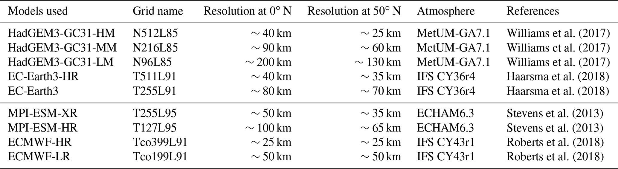
2.2 CERES-EBAF
The model-simulated TOA and SFC CREs for the December–January–February (DJF) and June–July–August (JJA) averaged months are evaluated against the CERES-EBAF satellite observational data (https://ceres-tool.larc.nasa.gov, last access: 3 April 2019). The CERES instrument aboard NASA's satellites aims at understanding the clouds and Earth's energy budget. The first CERES instrument was launched aboard NASA's Tropical Rainfall Measurement Mission (TRMM) in 1997 and thereafter similar instruments were flown aboard three satellite missions, namely Terra and Aqua satellites and Suomi National Polar-orbiting Partnership (S-NPP) satellite. The clear- and all-sky TOA and SFC fluxes are available at a 1×1∘ resolution for the period 2000–2016. For the fluxes at the TOA and SFC, the CERES_EBAF_TOA_Ed4.0 version (Loeb et al., 2009) and CERES_EBAF_Surface_Ed2.8 (Kato et al., 2013) are used, respectively. CERES cloud forcing and flux datasets have been used in a number of studies for model evaluations (Wang and Su, 2013, 2015; Stanfield et al., 2015; Calisto et al., 2014). For the analysis, the model data are also regridded to a 1×1∘ grid. However, in order to increase the number of cases with enhanced positive and negative phases of ENSO and NAO, we consider the whole time period in our simulations from 1982 to 2014, even though the observational reference period is shorter. In the era of both Terra and Aqua satellites (i.e. from 2002 onwards), both the global and regional uncertainties in the CERES-EBAF TOA and SFC fluxes are reduced dramatically. The typical overall uncertainty, after considering the uncertainties in the calibration, diurnal corrections and radiance-to-flux conversions in the TOA SW and LW, remain in the range of 2–5 W m−2. The uncertainties in the surface fluxes are higher, typically in the range 5–18 W m−2. The detailed data quality summaries are found at the following links:
-
https://ceres.larc.nasa.gov/documents/DQ_summaries/CERES_EBAF_Ed4.0_DQS.pdf (last access: 3 February 2019)
-
https://ceres.larc.nasa.gov/documents/DQ_summaries/CERES_EBAF-Surface_Ed4.0_DQS.pdf (last access: 26 May 2017)
2.3 ENSO analysis
ENSO is the leading mode of interannual climate variability in the tropics, where it has an impact on the Walker circulation and the local Hadley circulation, and thereby has a big response in the CREs (Cess et al., 2001a, b). To compute the CRE response to ENSO, first, the Niño3.4 index is computed to extract the positive and negative phases of El Niño. This index is based on the sea surface temperature (SST) anomalies over the Niño3.4 region (5∘ N–5∘ S, 170–120∘ W). When the SST anomalies over this region are positive (negative) and more (less) than 1 standard deviation, ENSO is considered to be in a stronger positive (negative) phase (denoted hereafter as ENP and ENN, respectively). This method is applied to all the models used in this study to extract the months when these phases are encountered. For our reference dataset, CERES, the positive and negative phases are chosen from observations (https://www.esrl.noaa.gov/psd/enso/, last access: 5 April 2019). The TOA and SFC cloud radiative fluxes associated with these phases are then computed. To extract the cloud response associated solely with ENP and ENN phases, the differences from the monthly climatological CREs are taken. This would give the change in the CREs during El Niño/La Niña years with respect to normal years. The ensemble mean of the CRE response from the Hi-res and Std-res models is evaluated.
2.4 NAO analysis
NAO is the most prominent mode of winter variability in the North Atlantic region. To evaluate the CREs associated with the positive and negative phases of NAO, the standard NAO index is calculated by taking the difference between normalized sea level pressure (SLP) anomalies between Ponta Delgada, Azores (southernmost point), Portugal, and Stykkishólmur, Iceland (northernmost point) (Stoner et al., 2009). To extract the stronger positive and negative phases of NAO in the observational reference dataset, the NAO indices are calculated using the SLP from ERA-Interim data. This study focuses on stronger- and weaker-than-normal NAO phases. If the NAO index is positive (negative) and is more (less) than 1 standard deviation, the NAO is considered to be in the stronger positive (negative) phase (NAOP/NAON). For this analysis, we consider the extended winter period from November to April. This method is followed to compute the NAO indices in all the models. As in the case of the ENSO analysis, to quantify the response of the NAO to the TOA and SFC CREs, the difference of the CREs associated with the phases from the climatological mean is taken. Here, since the focus is on the winter half of the year, the seasonal climatological mean is considered. Here, too, the CRE responses based on Hi-res and Std-res model setups are analyzed separately.
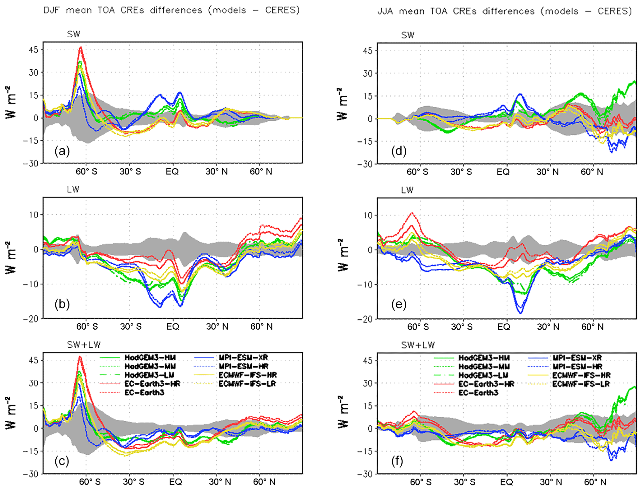
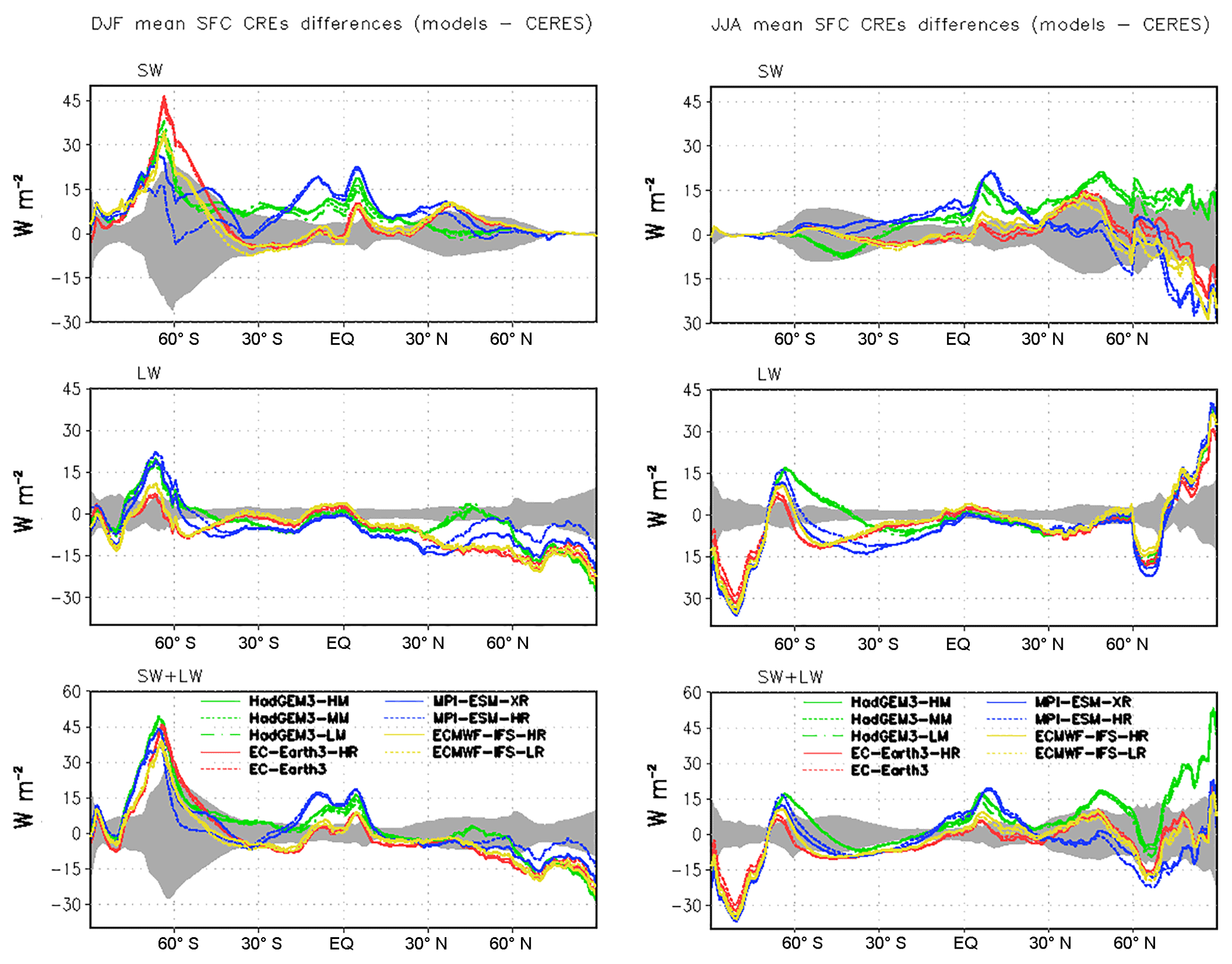
Figure 1The model-simulated SW, LW and combined TOA cloud radiative effects in W m−2 shown as differences from the CERES-EBAF observations for (a, b, c) DJF mean and (d, e, f) JJA mean. The green lines correspond to the simulations with the HadGEM3 model, red lines to the EC-Earth3 model, blue lines to the MPI-ESM model and yellow lines to the ECMWF model. The grey-coloured envelope indicates 1 standard deviation of CREs based on CERES, shown here as a measure of natural variability in the observations.
In this section, the statistical comparison and evaluation of TOA and SFC cloud radiative effects and their sensitivity to model resolution are presented in Figs. 1 to 4. The SW and LW components are evaluated separately for DJF mean (left) and JJA mean (right) seasons and are presented as zonally averaged differences from the observations. Also shown are the net CREs (i.e. SW + LW). The grey envelopes in Figs. 1 and 4 show 1 standard deviation of CREs in the CERES observations over the 16-year period, as a measure of natural interannual variability in the zonal means.
3.1 CREs at the TOA
In DJF, all models, irrespective of their resolution, overestimate the SW TOA CRE by 20–40 W m−2 over the bright and persistent decks of Southern Ocean clouds (Fig. 1, left). This overestimation is well above the expected variability seen in the observations (grey envelope). A clear distinction can be seen in the MPI-ESM model, where the lower-resolution simulation has the lowest positive bias compared to the other models. All the models underestimate the SW TOA CRE by 10 W m−2 over the convective regimes in the Southern Hemisphere (SH), while HadGEM3 setups better simulate this response, irrespective of their resolution. Over the tropical belt, the two models (HadGEM3 and MPI-ESM) show a positive bias by up to 15 W m−2, and the other models seem to have a slight negative bias. On the contrary, the LW CREs are underestimated by all the models over this region. Here, too, the biases are significantly higher than the observational variability. The standard-resolution versions of the respective models better simulate the LW effects in DJF mean over the tropical belt. The high biases in the SW CREs in the south are clearly seen in the combined response.
In JJA months, a large discrepancy is seen north of 30∘ N in the SW CREs (Fig. 1, right). The model resolution of the respective models does not play an important role in this case. While the HadGEM3 simulations have a strong positive bias, all the other models tend to have a more negative bias. This is also reflected in the combined CREs, as the biases in the LW tend to be relatively smaller. The model biases vary widely over the warm pool area in the western Pacific. While the HadGEM3 and MPI-ESM model simulations overestimate the TOA SW cloud radiative fluxes in the tropical monsoon belt, they underestimate the TOA LW fluxes by up to 15 W m−2. It is evident that, in both DJF and JJA averages, the opposite sign in the TOA SW and LW effects nearly compensates for the biases in the fluxes over the tropics in the net effects at the TOA.
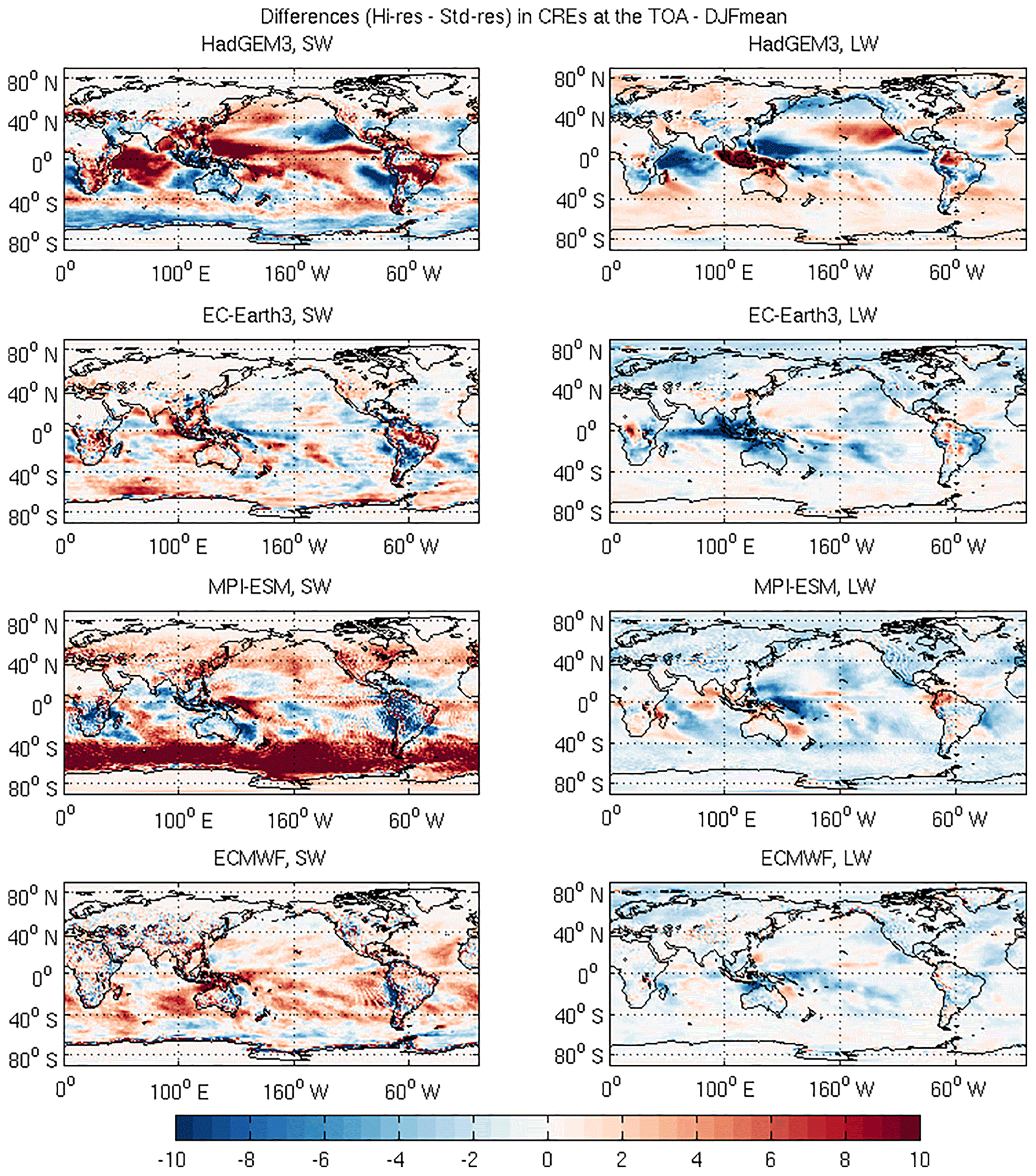
Figure 2Differences in the CREs at the TOA during DJF (W m−2) between the Hi-res and Std-res configurations of the respective models in the SW (left) and LW (right).
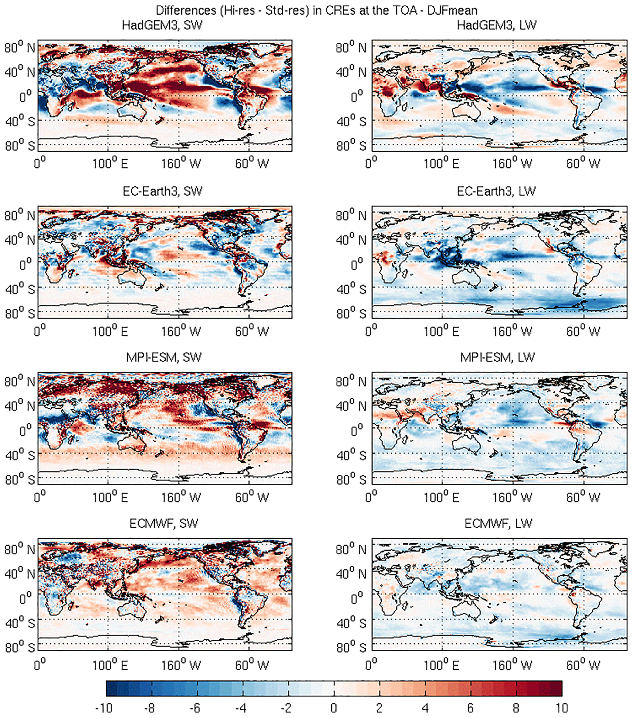
As can be seen in Fig. 1, when the zonal averaging of the CREs is performed, the differences between the high- and standard-resolution models remain low, mainly due to averaging out of over- and underestimations. Therefore, it looks as if the choice of the resolution does not seem to have a major impact on the simulation of the CREs. The regional differences emerge as we look in detail into the spatial patterns of the CRE differences between the Hi-res and Std-res setups of the respective models. This is presented in Figs. 2 and 3 at the TOA for the DJF and JJA months, respectively. It can be seen that the EC-Earth3 and the ECMWF models have lower differences, indicating insensitivity to the resolution. The Hi-res setup of MPI-ESM model is, however, strongly overestimating the SW response by around 15 W m−2 over the Southern Ocean compared to its corresponding standard-resolution setup during DJF mean months. Though a slight underestimation by the Hi-res setup is observed in the HadGEM3 model over this region, the major difference is observed over the tropics, where the Hi-res setup is overestimating the SW CRE over the tropical Pacific and Indian oceans compared to the respective Std-res setup. However, the Hi-res model configurations of the respective models seem to underestimate the CREs globally in the LW compared to their standard-resolution counterparts. The most notable underestimation is over the equatorial west Pacific. While the Hi-res EC-Earth3 and ECMWF model setups tend to slightly underestimate the LW CRE, the Hi-res HadGEM3 model setup tends to overestimate this over the southeast Asian region. A completely different picture can be seen in the JJA mean CREs at the TOA (Fig. 3). Strong differences in the SW CREs are simulated in the MPI-ESM and HadGEM3 models, with significant overestimation in Hi-res setups over the North Pacific in the HadGEM3 models and north of 40∘ N in the MPI-ESM model compared to their Std-res model counterparts. The impact of the resolution seems to be fairly negligible in the ECMWF model. The Hi-res setups of the respective models underestimate the LW CRE in general. This underestimation is prominent over southeast Asia and equatorial Pacific in the EC-Earth and HadGEM3 models. Stronger response to increased resolution is simulated over southern India and northern Africa in the Hi-res HadGEM3 model.
It is noteworthy that the cloud regimes that seem to be affected by increasing resolution are different in different models. For example, in DJF, the HadGEM3 models show largest differences in the convective ITCZ regions, while MPI-ESM over the Southern Ocean stratocumulus regions. The most drastic change in resolution occurs in the HadGEM3 models (from 200 to 50 km). This may have an impact on SST resampling and thus convection. In the case of Southern Ocean clouds, the increasing resolution in MPI-ESM may change the humidity PDFs (probability density functions) in a way that would change cloud fraction (since the relative humidity is already persistently high in this region). In addition, the lack of tuning in higher-resolution versions can further explain the observed differences.
3.2 CREs at the surface
The differences in the model-simulated CREs at the SFC from the observations are shown in Fig. 4 in the SW, LW and SW + LW averaged over DJF (left) and JJA (right) months. A similar picture, as observed at the TOA, can be seen at the SFC in SW CREs over the Southern Ocean clouds in the DJF season. All the models show a positive bias over this region, similar in magnitude to the TOA CREs. The MPI-ESM models tend to simulate a lower positive bias with the standard-resolution setup reducing this bias even more. Over the tropical belt, the models exhibit a similar variability, but a marginally stronger bias is simulated in SW CREs at the SFC compared to that what is seen at the TOA. A similar tendency compared to that at the TOA is observed in JJA mean SFC CREs in tropics and beyond 30∘ N. The differences are enhanced during DJF and JJA months in LW CREs at the SFC, when compared to that seen at the TOA. While all the models, irrespective of their resolutions, tend to simulate the LW CREs reasonably well over the tropics in both seasons, large discrepancies can be seen at higher latitudes. A strong overestimation is simulated by all the models in LW CREs south of 60∘ S and a strong underestimation north of 30∘ N. The EC-Earth and ECMWF models simulate a lower positive bias in LW CREs compared to the other model setups over the Southern Ocean in the mean DJF months. The JJA mean LW CREs are poorly simulated by all the models southward of 45∘ S and northward of 60∘ N. The biases in the SW CREs at the TOA and the surface are correlated, while they are less so in the LW. This is mainly due to the fact that the LW CRE at the surface is heavily dependent on the cloud base heights and the surface conditions. Both of these factors do not change significantly in the models for optically thicker clouds. In comparison, the different description of convection can heavily impact cloud top pressure and thus the LW TOA CREs.
During polar summers in both hemispheres, strong biases are observed in the surface SW CREs. These biases are most pronounced over the regions where seasonal sea-ice melt drives the intraseasonal variability in sea ice. The magnitude of these biases can reach up to 40 W m−2 over sea-ice regions near Antarctica and up to 30 W m−2 over the Arctic Ocean. The signs of the biases are however different in the both hemispheres during their respective summers. While the models mostly tend to underestimate the SW CRE over the Arctic in NH summer, they tend to overestimate it over Antarctica in the SH summer. Having a correct description of surface albedo in models is crucial to minimize these biases. However, it is evident that the models differ considerably from observations and from one another, as each model has its own formulation of sea-ice albedo (Koenigk et al., 2014); for example, a climatological annual cycle is used in EC-Earth3 models. This in turn has an impact on the formation of clouds through air–sea interaction processes. The biases in the LW CREs are also high in the polar regions at the surface, most likely originating from the biases in describing dominant atmospheric processes such as the strength of temperature inversions and heat and moisture transport (Medeiros et al., 2011; Woods et al., 2017). The higher positive bias north of 60∘ N in the HadGEM3 model simulations both in the SW CREs during JJA months at both the SFC and TOA results in a much higher positive bias compared to the other models in the net CREs.
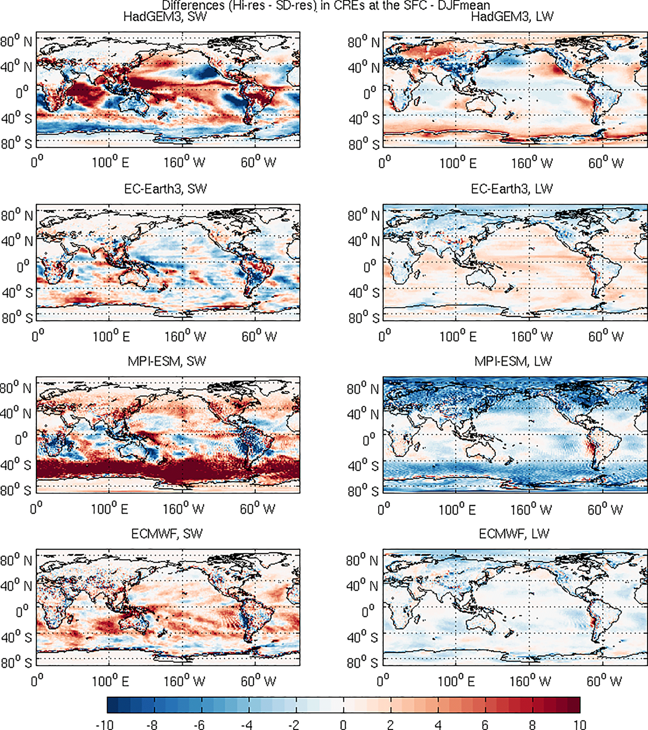
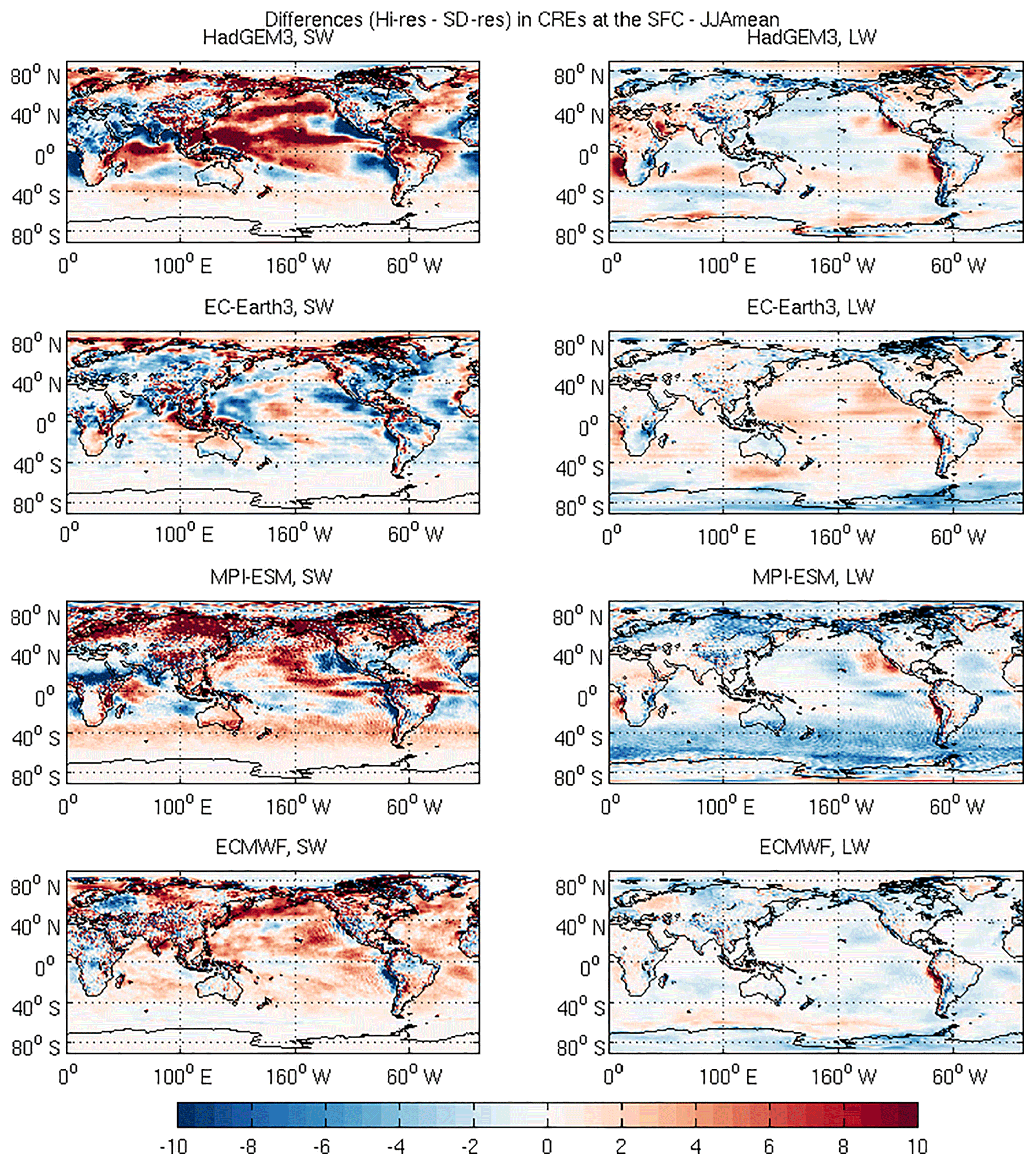
Similar to the TOA, the differences in spatial distribution in the SW CREs between the Hi-res and the Std-res model configurations are analyzed at the surface and are shown in Figs. A1 and A2 in Appendix A for mean DJF and JJA, respectively. It can be seen that the differences at the surface in the SW CREs are similar, both spatially and in magnitude to what is seen at the TOA in winter. However, large differences are seen in the surface LW CREs. As in the case of the TOA, the ECMWF model is insensitive to a change in resolution. The Hi-res setup of the MPI-ESM model significantly underestimates the LW CREs north of 40∘ N compared to its Std-res configuration. The DJF mean surface LW CRE biases are much smaller in EC-Earth3 model, but the Hi-res setup overestimates the LW forcing over the oceans and underestimates it over the continents. A strong overestimation is also seen in the Hi-res setup of the HadGEM3 model over the Southern Ocean and Eurasia. In summer, the SW CREs at the surface follow the same pattern as is seen at the TOA. However, the summer LW CRE biases at the surface are considerably weaker as compared to those in winter.
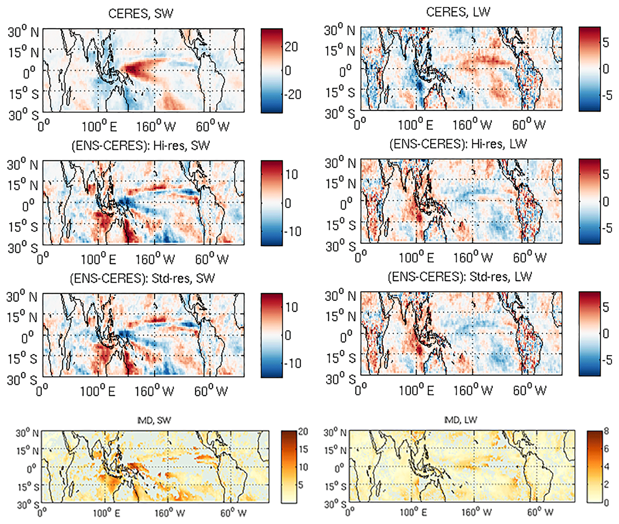
The TOA and SFC CREs associated with the ENP and ENN cases from model simulations are analyzed. The top row in Fig. 5 first shows the CREs associated with ENP from CERES-EBAF observations at the TOA in the SW (left panels) and LW (right panels). To investigate the simulated responses, the ensemble mean of the Hi-res and Std-res model configurations is analyzed. This would give us an understanding if increasing the spatial resolution results in an improvement of the response in the models. Hence, the second and third rows in Fig. 5 show the differences of the model ensemble mean of Hi-res and Std-res from the observations, respectively, and the intermodel differences are plotted in the bottom row. The intermodel differences are calculated as follows. At each grid point, if all nine model setups agree on the sign of bias with respect to the CERES observations, the absolute difference between the model setups showing the highest and lowest bias is reported as the intermodel difference. The regions, where all nine model setups do not agree in the sign of the bias, are marked in grey colour. Figure 6 shows the same but at the surface. Furthermore, Figs. 7 and 8 show similar responses but during the ENN case at the TOA and SFC, respectively.
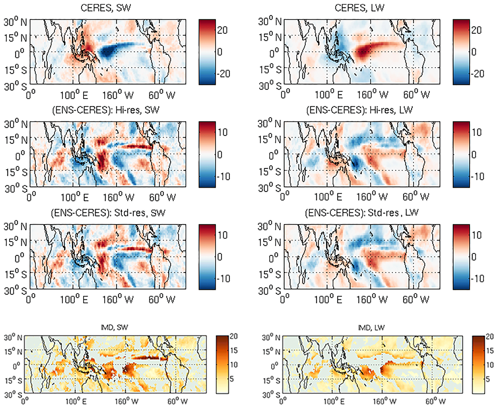
Figure 5The SW (left) and LW (right) cloud radiative fluxes at the TOA as a response to positive phase of ENSO (ENP) from the top row: CERES-EBAF observations; second row: the ensemble mean Hi-res; and third row: Std-res model-simulated differences of this response from observations. Bottom row: the ensemble intermodel differences in W m−2. The grey shaded areas are the regions where all the nine model setups do not agree with the sign of the bias.
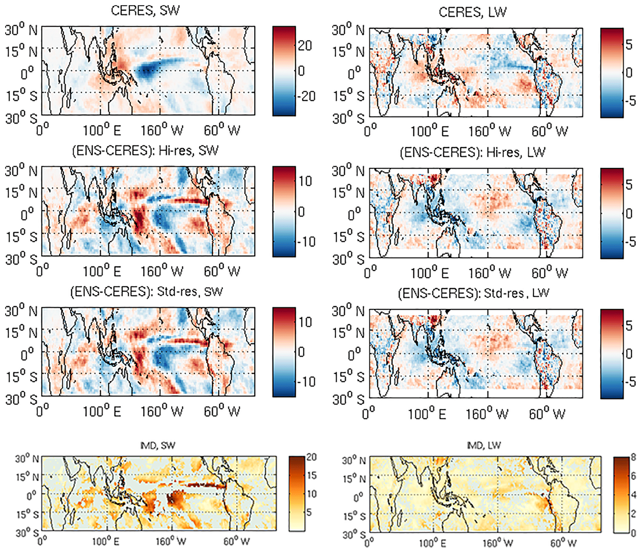
Figure 7The SW (left) and LW (right) cloud radiative fluxes at the TOA as a response to negative phase of ENSO from top row: CERES-EBAF observations; second row: the ensemble mean Hi-res; and third row: Std-res model-simulated differences of this response from observations. Bottom row: the ensemble intermodel differences in W m−2. The grey shaded areas are the regions where all the nine model setups do not agree with the sign of the bias.
4.1 The ENP case
In the ENP case, negative CRE anomalies (cooling) of up to 35 W m−2 over the western and central Pacific in the SW and positive anomalies (warming) of magnitude 20 W m−2 over the same region in the LW at the top of the atmosphere are observed. This is expected, because, during the positive phase of El Niño, the Walker circulation weakens, resulting in warmer ocean surface temperatures over the eastern and central Pacific, which favours increased deep convective and stratiform clouds in this region and reduced cloud cover over the southeast Asian regions (Fig. 9), and the opposite is observed during the La Niña phase (Eastman et al., 2011; Park and Leovy, 2004). This induces enhanced cooling/warming in the SW/LW, respectively, not only at the TOA but also at the surface in the SW. The LW signal at the surface during ENP is considerably weaker, as for similar convective systems; the cloud base heights over the oceans do not change significantly in the models.
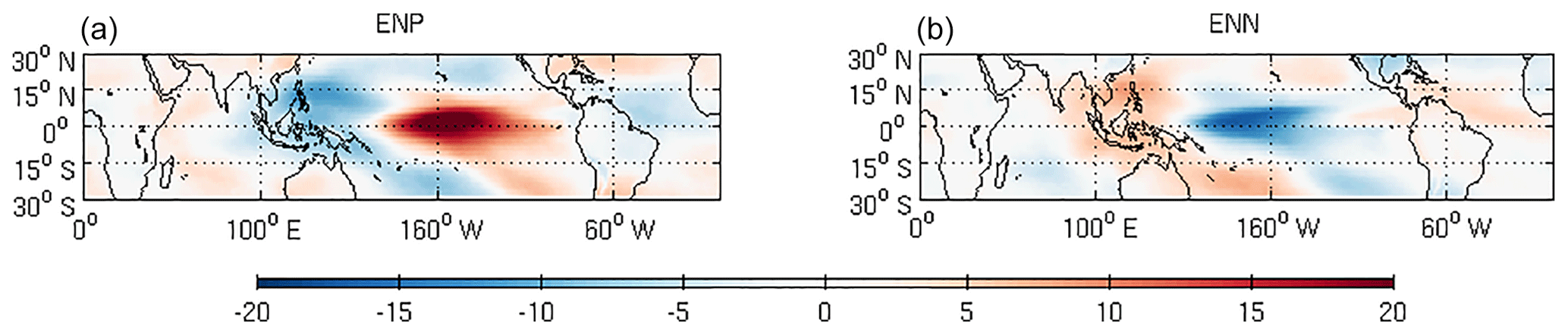
Figure 9Ensemble model mean of simulated total cloud fraction anomalies (%) as a response to the positive phase of ENSO (a) and negative phase of ENSO (b).
It is observed that the pattern correlations (i.e. the Pearson product–moment coefficient of linear correlation) with CERES observations in the tropical belt (30∘ N–30∘ S) are approximately above 0.75 for all the models irrespective of their resolution (not shown here). This suggests that the models realistically reproduce the spatial variability of the CRE response. However, the magnitude of this response and the location of the peak cooling/warming vary substantially regionally among the models, as can be seen from the differences of the ensemble model means from the observations.
Both model setups, i.e. Hi-res and Std-res, simulate the peak cooling region in SW cloud radiative fluxes at the TOA and surface over the western and central Pacific during ENP reasonably well. The multi-model ensemble mean strongly overestimates the TOA and surface SW CREs north and south of the peak cooling region over the western Pacific by around 10 W m−2 and underestimates the cooling by around 5 W m−2 over the central Pacific. The Hi-res model setups simulate a stronger bias than the Std-res models over this region. Both the Hi-res and the Std-res models slightly overestimate the cooling over the tropical Indian Ocean and underestimate the warming over SE Asia at the surface and at the TOA. Over the SE Asian region, the underestimation at the TOA is around 5–8 W m−2, more so, in the Hi-res ensemble model mean.
The models, irrespective of their resolution, tend to simulate the peak ENSO response over the central Pacific to the TOA LW cloud radiative fluxes reasonably well. The LW biases over the southwest Pacific are marginally stronger in the Hi-res compared to the Std-res ensemble mean model configurations. An opposite sign in the biases is observed in the LW CREs compared to the SW CREs at the TOA. Although the model biases in the LW at the TOA during the positive phase of ENSO are small, clear hemispherical differences can be seen over the central and eastern Pacific at the TOA in the ENP case characterized by negative biases north of 5∘ N and positive biases south of 5∘ N. Considering that the models do capture the broad spatial pattern in the CRE response but at the same time exhibit wave-like structures in the SW biases and hemispheric nature of LW biases, it can be due to the fact that the shift of Walker circulation in the models is not followed with corresponding changes in cloud optical and physical characteristics. The signal in the LW CREs at the surface during ENP is muted and hence are the biases.
Large variability of up to 20 W m−2 can be seen in the intermodel differences on the simulation of TOA and surface SW CREs associated with ENP and are mainly over the Pacific. The model bias is higher in the SW CREs compared to the LW CREs. The TOA biases are consistent with those observed in the set of CMIP5 models carried out with varying resolutions forced by AMIP (Atmospheric Model Intercomparison Project) SSTs (Wang and Su, 2015). These strong model over-/underestimations over the tropical convective regions could be because of the discrepancies in the simulation of convective clouds (Wang and Su, 2013), as models have a tendency to produce optically thicker and deeper clouds compared to observations, whereas thin cirrus is prevalent in observations in those regions.
4.2 The ENN case
In the ENN case, a signal of opposite sign to that of ENP is observed with positive CREs in the SW at the TOA and the surface and negative anomalies in the LW at the TOA over the western and central Pacific. Over southeast Asia, a weaker signal is observed. Though the models marginally underestimate the warming in the SW associated with ENN at the TOA and the surface, they simulate the response in the LW at the TOA reasonably well. The Hi-res model setups tend to slightly intensify this underestimation in the SW compared to the Std-res model setups. The LW CRE associated with ENN at the surface is weaker. No notable improvements can be seen in simulating the cloud response in the LW using Hi-res model setups. The intermodel differences are smaller in the simulation of the TOA and surface LW CREs compared to the SW.
4.3 The regional absolute biases
In order to better understand the role of varying spatial resolution locally, we further examine individual models under their high- and standard-resolution setups. Figure 10 shows the average absolute biases in TOA and SFC CREs in the SW and LW during the positive and negative phases of ENSO, with reference to CERES, over the Niño3.4 region (170–120∘ W, 5∘ N–5∘ S). It can be seen that the absolute biases across the models are high in the SW at the TOA and SFC and in the LW at the TOA during the positive phase of ENSO, particularly in the HadGEM3 and EC-Earth3 models. The uncertainty bars show 1 standard deviation in the CERES anomalies for the respective cases as a measure of the variability in the observation data. It is to be noted that, in all cases, the observed biases over the selected region remain below the variability in the CERES data. The Hi-res setups of HadGEM3 and EC-Earth models have a lower bias compared to their Std-res setups. The opposite is seen in MPI-ESM models. ECMWF models, irrespective of their resolution, show a similar bias.
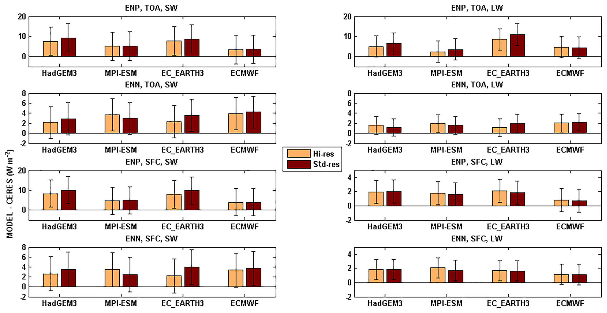
Figure 10Average absolute errors in the Hi-res and Std-res of the model versions with reference to CERES averaged over the Niño3.4 region (170–120∘ W, 5∘ N–5∘ S) in the SW (left) and LW (right) during the enhanced positive and negative phases of El Niño at the TOA (rows 1–2) and at the SFC (rows 3–4). The uncertainty bars show 1 standard deviation in the CERES anomalies for the respective cases as a measure of the variability in the observation data.
The TOA and SFC CREs associated with NAOP from observations are shown in top row of Figs. 11 and 12, respectively. The second and third rows show the ensemble mean difference of the response simulated in Hi-res and Std-res models with the observations, respectively, and the intermodel differences are shown in the bottom row. Figures 13 and 14 show the same but for the NAON case. The SW (left) and LW (right) components of the total CREs are shown separately in each of the NAOP and NAON cases.
5.1 The NAOP case
During the positive phase, as the polar vortex strengthens trapping the cold air in the central Arctic, the winter storms in the North Atlantic penetrate further to the north, with their remnants reaching deep over the northern Norwegian and Greenland seas. The northeast Atlantic is usually persistently cloud covered. However, the additional transport of heat and moisture brought about by winter storms leads to increased opacity of these cloud systems. This is evident in the slight decrease in the TOA and surface SW CRE. The increased opacity of clouds leads to additional reflection of solar radiation back to the space, while the clouds also emit at warmer temperatures than normal. LW CRE is especially stronger over Scandinavia and the Norwegian Sea at the TOA. The LW CRE anomalies over the North Atlantic are quite muted at the surface, whereas the Greenland and Canadian sectors of the Arctic show increased LW CREs. This is mainly due to the fact that, in contrast to open oceanic waters in the North Atlantic, clouds can exert strong LW forcing over the ice- and snow-covered areas in the Arctic. Over the Mediterranean region and Iberian Peninsula, colder and drier conditions prevail during the NAOP case due to the northward shift of the storm tracks. This results in a significant reduction in cloud cover over this region, as can be seen in the model-simulated NAO-related total cloud fraction anomalies during this phase (Fig. 15), which are also consistent with the previous studies (Chaboureau and Claud, 2006; Trigo et al., 2002). Clearer conditions result in an increase in SW CRE and a decrease in LW CRE at the TOA and at the surface.
The Hi-res and Std-res model ensemble mean differences against CERES observations are generally quite low (below ±5 W m−2) and do not exceed 1 standard deviation of the CRE anomalies observed in the CERES data over the majority of the regions (not shown). The models capture the spatial cloud radiative response to the positive phases of the NAO quite well. For example, the models, irrespective of their resolution, simulate the response reasonably well over the North Atlantic, over Scandinavia and over the Mediterranean at the TOA in both SW and LW and at the SFC in the SW. The models overestimate the cooling by 3–4 W m−2 over continental Europe in the SW at the TOA and SFC. The LW TOA CRE is, on the other hand, underestimated over this region. However, strong discrepancies can be noted in the SFC LW CREs with models overestimating the response by more than 5 W m−2 over northern Europe. Strong underestimation of similar magnitude in the LW CRE at the surface can be noted in the Canadian sector of the Arctic Ocean and also over Greenland.
The CRE biases in the Hi-res and Std-res model setups do not seem to be strikingly different from one another at a first glance. However, the Hi-res models seem to amplify the positive SW bias over eastern Europe at the SFC during NAOP compared to the Std-res model ensemble mean. On the other hand, the Hi-res models better simulate the TOA LW CREs over continental Europe. No notable improvement is seen in the SFC LW CREs with resolution. The intermodel differences are of the same magnitude as those of the under- and overestimations in the CRE response at the TOA. The SW and LW biases are, respectively, much higher at the surface over continental Europe and over Scandinavia.
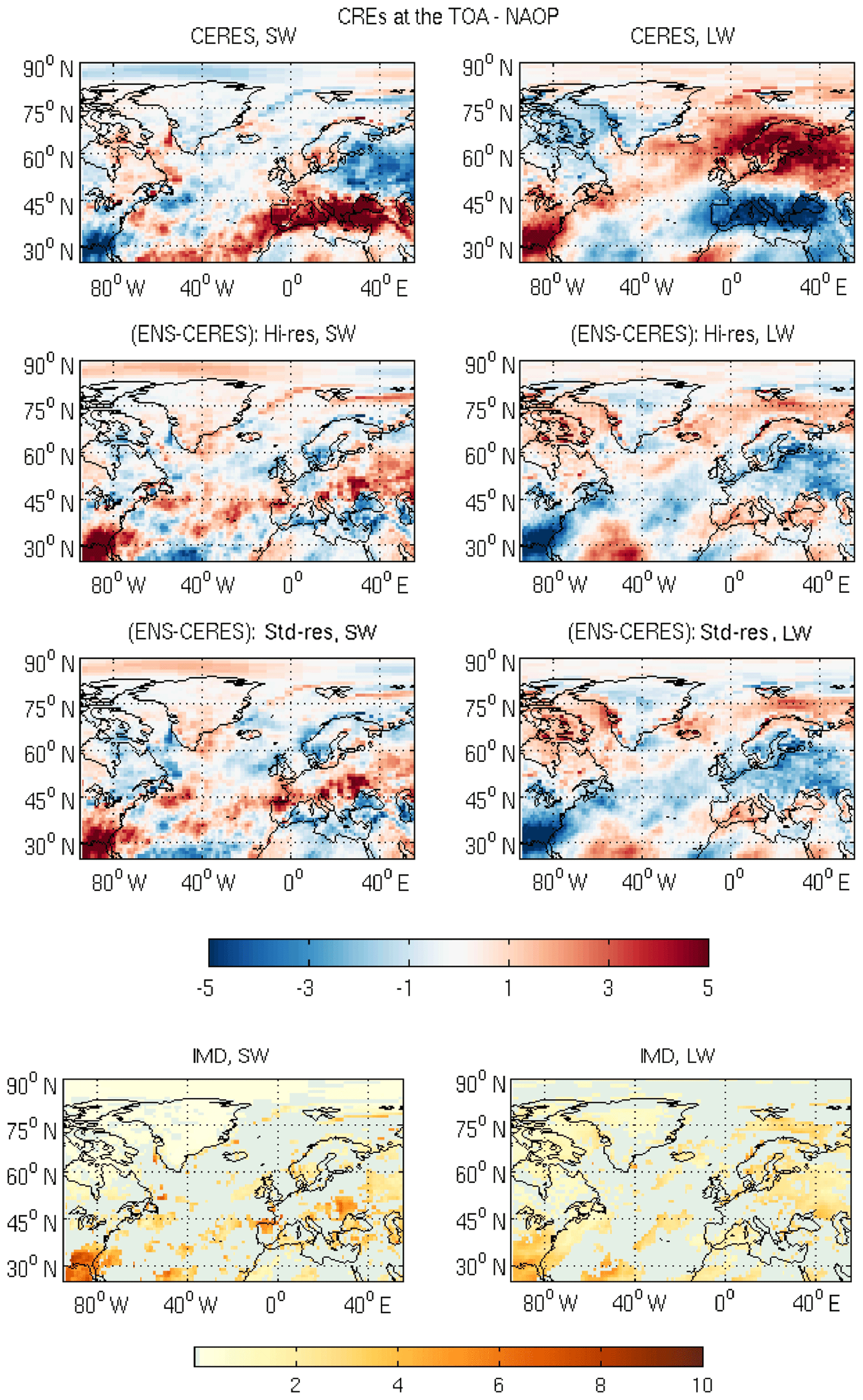
Figure 11The SW (left) and LW (right) cloud radiative fluxes at the TOA as a response to positive phase of NAO from top row: CERES observations; second row: the ensemble mean Hi-res; and third row: Std-res model-simulated differences of this response from observations. Bottom row: the ensemble intermodel differences in W m−2. The grey shaded areas are the regions where all the nine model setups do not agree with the sign of the bias.
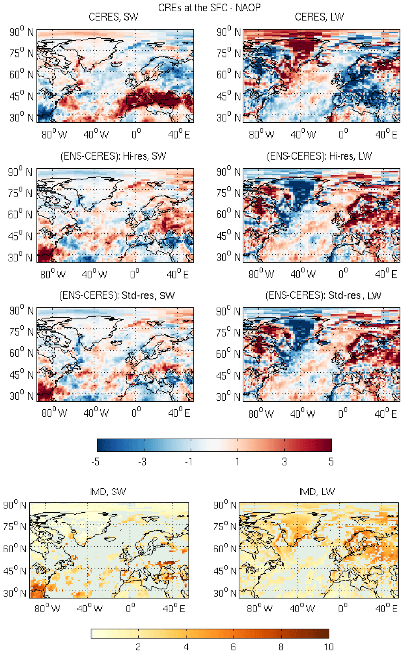
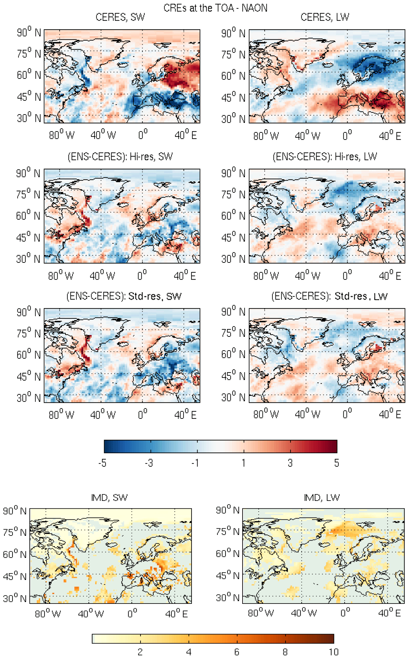
Figure 13The SW (left) and LW (right) cloud radiative fluxes at the TOA as a response to negative phase of NAO from top row: CERES observations; second row: the ensemble mean Hi-res; and third row: Std-res model-simulated differences of this response from observations. Bottom row: the ensemble intermodel differences in W m−2. The grey shaded areas are the regions where all the nine model setups do not agree with the sign of the bias.
5.2 The NAON case
In the NAON case (Fig. 13), the winter storms are not as intense and do not penetrate deeper into the northern North Atlantic as the cold air outbreaks from the Arctic over the northern high latitudes and midlatitudes prevail, shifting the zonal temperature gradient southwards. As a result, the TOA SW CRE is higher than usual over northern midlatitudes, and the TOA LW CRE is lower than usual as the clouds emit at the colder temperatures, especially over Scandinavia. The LW CRE at the surface is decreased over Greenland and the Canadian Arctic and increased over the Eurasian Arctic (Fig. 14). This response is opposite to that observed in the NAOP case. The CRE response in the Mediterranean region is also, as expected, opposite to that of the NAOP case.
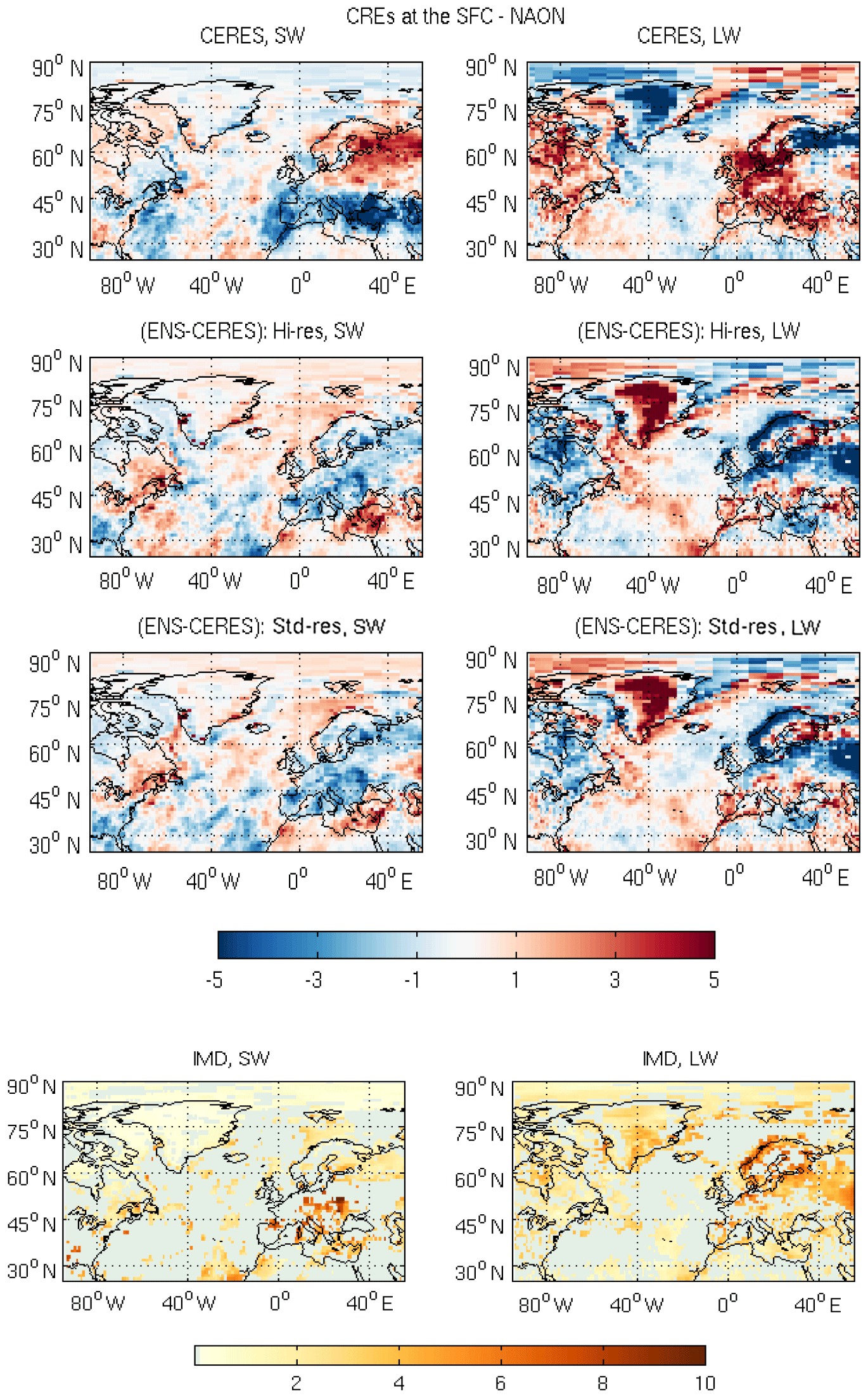
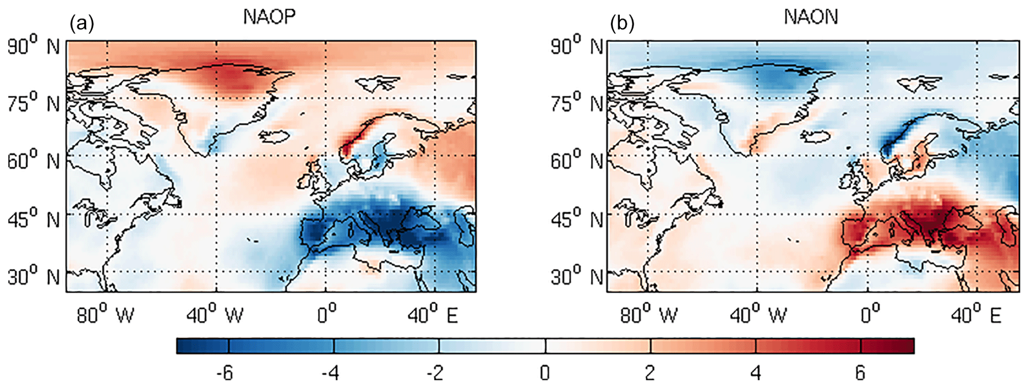
Figure 15Ensemble mean of model-simulated total cloud fraction anomalies (%) as a response to the (a) positive phase of NAO and (b) negative phase of NAO.
Both at the TOA and the SFC, though the biases are small in the SW CREs over the Atlantic and Scandinavia, the models underestimate the SW CREs over continental Europe by −4 W m−2. The models simulate the LW CREs at the TOA reasonably well; however, marginal underestimation in the cooling in the North Atlantic in LW CREs at the TOA can be noted. At the SFC, the biases in the LW CREs are highest over northern continental Europe, Greenland and along the west coast of Norway but are of opposite sign, in that the models underestimate CREs over northern Europe and the west coast of Europe and overestimate it over Greenland (locally exceeding 5 W m−2). Over the Eurasian and Canadian Arctic regions, the biases in the surface LW CREs are of opposite sign to that of the NAOP case.
An improvement in the SW CREs at the TOA can be noted in the Hi-res model ensemble mean over continental Europe at the TOA and SFC. Though there is a marginal improvement in the LW CREs at the TOA over North Atlantic, no notable differences are seen at the SFC. The intermodel differences, like in the case of NAOP, are much higher in the SW than the LW at the TOA and SFC, particularly over continental Europe. The differences are the same or even lower in magnitude compared to that of the under- and overestimations of the CRE response.
5.3 The absolute regional biases
Figure 16 shows the absolute biases in the high- and standard-resolution model setups for the different phases of NAO over Europe (30–75∘ N, 40∘ W–40∘ E). This region is active with winter storms during the positive phases of the NAO, which eventually transport heat and moisture to the northernmost latitudes. Here, it has to be noted that the biases are comparatively smaller than the biases observed in the ENSO cases. Further, there is no noticeable improvement with increased resolution. This indicates that improving the surface description and treatment (e.g. surface snow and ice variability) in models might be more important than increasing only the horizontal resolution for cloud processes. The uncertainty bars show that the biases over the selected region remain below the variability in the CERES data. This means that the model biases are not significant.

Figure 16Average absolute errors in the Hi-res and Std-res of the model versions with reference to CERES averaged over Europe (30–75∘ N, 40∘ W–40∘ E) in the SW (left) and LW (right) during the enhanced positive (NAOP) and negative (NAON) phases of NAO at the TOA (rows 1–2) and at the SFC (rows 3–4). The uncertainty bars show 1 standard deviation in the CERES anomalies for the respective cases as a measure of the variability in the observation data.
In the present study, we evaluated four global climate models at different spatial resolutions to assess how well they simulate CREs, both at the top of the atmosphere and at the surface, as well as their shortwave and longwave components. The focus is placed on evaluating cloud radiative response to two leading modes of natural variabilities, namely ENSO and NAO, allowing process-oriented evaluations. The simulations from the high- and standard-resolution model setups were contrasted to investigate if any value can be added by increasing the spatial resolution of the different models. The retrievals of CREs from CERES instruments aboard a series of satellites were used as the observational reference. The following conclusions can be drawn from the evaluations.
- a.
The largest disagreement between models and observations occurs over the polar regions, both at the TOA and the SFC, and especially over the locations where seasonal sea-ice variability is strongest. The surface SW CRE plays an important role during the melt season. The models, however, overestimate this forcing by up to 35 W m−2 over the coastal Antarctic and underestimate it by 20–30 W m−2 over the Arctic. This will have an implication for quantifying the cloud feedbacks on the sea ice and estimating future changes in sea ice during the melt season.
- b.
The zonally averaged CREs do not seem to be resolution dependent. This means that all the models follow a similar response irrespective of the resolution in most regions. However, regional differences emerge when looking at the spatial patterns of the forcings. Here, it is seen that different cloud regimes are affected by increasing resolution in different models.
- c.
The spatial patterns of cloud radiative response to ENSO in the tropical belt is simulated reasonably well by the models, with spatial correlations up to 0.75. However, strong biases in the magnitude of this response are noted. The model biases are generally half as large as those of the actual cloud radiative response seen in the CERES data for the ENSO cases (5–10 W m−2) at both the TOA and the surface, with Hi-res model setups simulating a stronger bias than the respective Std-res models. The biases in the LW CRE tend to be smaller than in the SW CRE. The intermodel differences in the SW CRE at the TOA and surface over the convectively active regions are stronger, nearly of the same order as the actual response. The intermodel differences in the LW CRE are lower at the surface during both ENP and ENN, typically within a few W m−2. This suggests that the parameterization of SW radiative transfer and the treatment of cloud optical properties vary strongly among the models. The large-scale organization of convection and associated cloud types can also be different.
- d.
In the case of NAO, the model biases are less than observational uncertainties and also well within the observational variability (less than 1σ) in the CREs. The spatial patterns of the response are also simulated quite well by the models during the positive and negative phases of the NAO. The biases in the surface LW CREs have a strong meridional character, in that they are of opposite sign over the eastern and western parts of the Arctic across 20∘ W and also have the opposite sign of that of the cloud radiative response observed in the CERES data.
- e.
The average absolute biases over the Niño3.4 region for the ENP and ENN cases and over Europe (30–75∘ N, 40∘ W–40∘ E) for the NAOP and NAON cases are investigated in the high- and standard-resolution setups of each model. The absolute biases in both cases are well below the variability in the observational data. The average biases in the case of NAO are smaller than the biases seen over the Niño3.4 region. The Hi-res setup of HadGEM3 and EC-Earth3 models has a lower bias compared to their Std-res counterparts over the Niño3.4 region, whereas an opposite signal is seen in MPI-ESM models. ECMWF model setups exhibit the same biases irrespective of the resolution.
From this study, it is clear that the well-known issue of the large biases in SW CREs over the polar regions during the melt season does not improve by increasing the resolution of the models chosen here. This would require improvements not only in the parameterization schemes involving the microphysical properties of clouds but also in the surface description. Analysis of the spatial pattern of the TOA SW CREs during winter reveals that different cloud regimes are affected drastically with a change in resolution in MPI-ESM and HadGEM3 models. For example, the Hi-res HadGEM3 model shows an overestimation over the convective ITCZ regions compared to its Std-res counterpart, and this may have an impact on SST resampling and thus convection. On the other hand, the Hi-res MPI-ESM overestimates the CREs over the Southern Ocean stratocumulus region and this may have an impact on the cloud fraction. The observed differences can be attributed to the lack of tuning in higher-resolution versions. Though the models tend to simulate the spatial variability in cloud radiative response to ENSO and NAO variability, they vary widely in the magnitude of the response. The CRE biases associated with the NAO phase are smaller compared to those with the ENSO phase. Although some improvements can be seen regionally, it is difficult to identify patters that hold across all models. Hence, it can be concluded that improving the physical parameterization schemes rather than increasing the resolution is perhaps important in better simulating the CREs. However, it has to be noted that these are atmospheric-only simulations and the impact may be different in the presence of coupled climate models.
Access to the model output data used in this study will be available through the European Research Council Horizon 2020 PRIMAVERA project (https://www.primavera-h2020.eu/modelling/, last access: 24 April 2019). More information regarding model configurations and data availability are available from the authors upon request.
MAT performed the analysis and drafted the paper. AD and TK helped in the interpretation of the results. The output for the respective models used in this paper was provided by KW, MR, CR and KL. All the authors contributed to the revision of the paper text.
The authors declare that they have no conflict of interest.
This study was financially supported by PRIMAVERA (PRocess-based climate sIMulation: AdVances in high resolution modelling and European climate Risk Assessment), a Horizon 2020 project funded by the European Commission.
This paper was edited by Klaus Gierens and reviewed by two anonymous referees.
Baker, N. C. and Taylor, P. C.: A framework for evaluating climate model performance metrics, J. Climate, 29, 1773–1782, https://doi.org/10.1175/JCLI-D-15-0114.1, 2016. a
Calisto, M., Folini, D., Wild, M., and Bengtsson, L.: Cloud radiative forcing intercomparison between fully coupled CMIP5 models and CERES satellite data, Ann. Geophys., 32, 793–807, https://doi.org/10.5194/angeo-32-793-2014, 2014. a
Cess, R. D., Zhang, M., Wielicki, B. A., Young, D. F., Zhou, X. L., and Nikitenko, Y.: The influence of the 1998 El Niño upon cloud-radiative forcing over the Pacific warm pool, J. Climate, 14, 2129–2137, 2001a. a
Cess, R. D., Zhang, M. H., Wang, P. H., and Wielicki, B. W.: Cloud structure anomalies over the tropical Pacific during the 1997/98 El Niño, Geophys. Res. Lett., 28, 4547–4550, https://doi.org/10.1029/2001GL013750, 2001b. a
Chaboureau, J.-P. and Claud, C.: Satellite-based climatology of Mediterranean cloud systems and their association with large-scale circulation, J. Geophys. Res., 111, D01102, https://doi.org/10.1029/2005JD006460, 2006. a
Doi, T., Vecchi, G. A., Rosati, A. J., and Delworth, T. L.: Biases in the Atlantic ITCZ in seasonal-interannual variations for a coarse- and a high-resolution coupled climate model, J. Climate, 25, 5494–5511, https://doi.org/10.1175/JCLI-D-11-00360.1, 2012. a
Eastman, R., Warren, S. G., and Hahn, C. J.: Variations in cloud cover and cloud types over the ocean from surface observations, 1954–2008, J. Climate, 24, 5914–5934, https://doi.org/10.1175/2011JCLI3972.1, 2011. a
Ferraro, R., Waliser, D. E., Gleckler, P., Taylor, K. E., and Eyring, V.: Evolving Obs4MIPs to support phase 6 of the Coupled Model Intercomparison Project (CMIP6), B. Am. Meteorol. Soc., 96, https://doi.org/10.1175/BAMS-D-14-00216.1, 2015. a
Flato, G., Marotzke, J., Abiodun, B., Braconnot, P., Chou, S. C., Collins, W., Cox, P., Driouech, F., Emori, S., Eyring, V., Forest, C., Gleckler, P., Guilyardi, E., Jakob, C., Kattsov, V., Reason, C., and Rummukainen, M.: Evaluation of Climate Models, in: Climate Change 2013: The Physical Science Basis. Contribution of Working Group I to the Fifth Assessment Report of the Intergovernmental Panel on Climate Change, edited by: Stocker, T. F., Qin, D., Plattner, G.-K., Tignor, M., Allen, S. K., Boschung, J., Nauels, A., Xia, Y., Bex, V., and Midgley, P. M., Cambridge University Press, Cambridge, United Kingdom and New York, NY, USA, 2013. a
Haarsma, R., le Sager, P., van den Oord, G., Bakhshi, R., van Noye, T., van Weele, M., von Hardenberg, J., Davini, P., Corti, S., Acosta, M., Bretonnière, P.-A., Caron, L.-P., Castrillo, M., Exarchou, E., Ruprich-Robert, Y., Tourigny, E., Wyser, K., Koenigk, T., and Fladrich, U.: PRIMAVERA versions of EC-Earth: EC-Earth3P and EC-Earth3P-HR. Description, model performance, data handling and validation, Geosci. Model Dev. Discuss., in preparation, 2018. a, b
Haarsma, R. J., Roberts, M. J., Vidale, P. L., Senior, C. A., Bellucci, A., Bao, Q., Chang, P., Corti, S., Fuckar, N. S., Guemas, V., von Hardenberg, J., Hazeleger, W., Kodama, C., Koenigk, T., Leung, L. R., Lu, J., Luo, J.-J., Mao, J., Mizielinski, M. S., Mizuta, R., Nobre, P., Satoh, M., Scoccimarro, E., Semmler, T., Small, J., and von Storch, J.-S.: High Resolution Model Intercomparison Project (HighResMIP v1.0) for CMIP6, Geosci. Model Dev., 9, 4185–4208, https://doi.org/10.5194/gmd-9-4185-2016, 2016. a, b, c
Hodges, K. I., Lee, R. W., and Bengtsson, L.: A comparison of extratropical cyclones in recent re-analyses ERA-Interim, NASA MERRA, NCEP CFSR, JRA-25, J. Climate, 24, 4519–4528, https://doi.org/10.1175/2011JCLI4137.1, 2011. a
Karlsson, K.-G. and Devasthale, A.: Inter-comparison and evaluation of the four longest satellite-derived cloud climate data records: CLARA-A2, ESA Cloud CCI V3, ISCCP-HGM, and PATMOS-x, Remote Sensing, 10, 1567, https://doi.org/10.3390/rs10101567, 2018. a
Kato, S., Loeb, N. G., Rose, F. G., Doelling, D. R., Rutan, D. A., Caldwell, T. E., Lisan, Y., and Weller, R. A.: Surface irradiances consistent with CERES-derived top-of-atmosphere shortwave and longwave irradiances, J. Climate, 26, 2719–2740, 2013. a
Kennedy, J., Titchner, H., Rayner, N., and Roberts, M.: input4MIPs.MOHC.SSTs and SeaIce.HighResMIP.MOHC-HadISST-2-2-0-0-0. Version 20170505, Earth System Grid Federation, https://doi.org/10.22033/ESGF/input4MIPs.1221, 2017. a
Koenigk, T., Devasthale, A., and Karlsson, K.-G.: Summer Arctic sea ice albedo in CMIP5 models, Atmos. Chem. Phys., 14, 1987–1998, https://doi.org/10.5194/acp-14-1987-2014, 2014. a
Loeb, N. G., Wielicki, B., Doelling, D. R., Smith, G. L. S., Keyes, D. F., Kato, S., Manalo-Smith, N., and Wong, T.: Toward optimal closure of the Earth's top-of-atmosphere radiation budget, J. Climate, 22, 748–766, 2009. a
Lu, J., Chen, G., Leung, L. R., Burrows, A., Yang, Q., Sakaguchi, K., and Hagos, S.: Towards the dynamical convergence on the jet stream in aquaplanet AGCMs, J. Climate, 28, 6763–6782, 2015. a
Masson, S., Terray, P., Madec, G., Luo, J.-J., Yamagata, T., and Takahashi, K.: Impact of intra-daily SST variability on ENSO characteristics in a coupled mode, Clim. Dynam., 39, 681–707, 2012. a
Medeiros, B., Deser, C., Tomas, R. A., and Kay, J.: Arctic inversion strength in climate models, J. Climate, 24, 4733–4740, https://doi.org/10.1175/2011JCLI3968.1, 2011. a
Murakami, H., Vecchi, G. A., Underwood, S., Delworth, T. L., Wittenberg, A. T., Anderson, W. G., Chen, J.-H., Gudgel, R. G., Harris, L. M., Lin, S.-J., and Zeng, F.: Simulation and prediction of Category 4 and 5 hurricanes in the High-Resolution GFDL HiFLOR coupled climate model,, J. Climate, 28, 9058–9079, https://doi.org/10.1175/JCLI-D-15-0216.1, 2015. a
Park, S. and Leovy, C. B.: Marine low-cloud anomalies associated with ENSO, J. Climate, 17, 3448–3469, https://doi.org/10.1175/1520-0442(2004)017<3448:MLAAWE>2.0.CO;2, 2004. a
Reichler, T. and Kim, J.: How well do coupled models simulate today's climate?, B. Am. Meteorol. Soc., 89, 303–311, https://doi.org/10.1175/BAMS-89-3-303, 2001. a
Roberts, C. D., Senan, R., Molteni, F., Boussetta, S., Mayer, M., and Keeley, S. P. E.: Climate model configurations of the ECMWF Integrated Forecasting System (ECMWF-IFS cycle 43r1) for HighResMIP, Geosci. Model Dev., 11, 3681–3712, https://doi.org/10.5194/gmd-11-3681-2018, 2018. a, b
Sakaguchi, K., Leung, L. R., Zhao, C., Yang, Q., Lu, J., Hagos, S., Ringler, T. D., Rauscher, S. A., and Dong, L.: Exploring a multi-resolution approach using AMIP simulations, J. Climate, 28, 5549–5574, 2015. a
Shaevitz, D., Camargo, S. J., Sobel, A. H., Jonas, J. A., Kim, D., Kumar, A., LaRow, T. E., Lim, Y.-K., Murakami, H., Reed, K., Roberts, M. J., Scoccimarro, E., Vidale, P. L., Wang, H., Wehner, M. F., Zhao, M., and Henderson, N.: Characteristics of tropical cyclones in high-resolution models in the present climate, J. Adv. Model. Earth Sy., 6, 1154–1172, https://doi.org/10.1002/2014MS000372, 2014. a, b
Stanfield, R. E., Dong, X., Xi, B., Del-Genio, A. D., Minnis, P., Doelling, D., and Loeb, N.: Assessment of NASA GISS CMIP5 and Post-CMIP5 simulated clouds and TOA radiation budgets using satellite observations. Part II: TOA radiation budget and CREs, J. Climate, 28, 1842–1864, https://doi.org/10.1175/JCLI-D-14-00249.1, 2015. a
Steiner, A. K., Lackner, B. C., and Ringer, M. A.: Tropical convection regimes in climate models: evaluation with satellite observations, Atmos. Chem. Phys., 18, 4657–4672, https://doi.org/10.5194/acp-18-4657-2018, 2018. a
Stephens, G., Winker, D., Pelon, J., Trepte, C., Vane, D., Yuhas, C., L'Ecuyer, T., and Lebsock, M.: CloudSat and CALIPSO within the A-Train: Ten years of actively observing the earth system, B. Am. Meteorol. Soc., 99, 569–581, https://doi.org/10.1175/BAMS-D-16-0324.1, 2018. a
Stevens, B., Giorgetta, M., Esch, M., Mauritsen, T., Crueger, T., Rast, S., Salzmann, M., Schmidt, H., Bader, J., Block, K., Brokopf, R., Fast, I., Kinne, S., Kornblueh, L., Lohmann, U., Pincus, R., Reichler, T., and Roeckner, E.: Atmospheric component of the MPI-M Earth System Model: ECHAM6, J. Adv. Model. Earth Sy., 5, 146–172, 2013. a, b
Stevens, B., Fiedler, S., Kinne, S., Peters, K., Rast, S., Müsse, J., Smith, S. J., and Mauritsen, T.: MACv2-SP: a parameterization of anthropogenic aerosol optical properties and an associated Twomey effect for use in CMIP6, Geosci. Model Dev., 10, 433–452, https://doi.org/10.5194/gmd-10-433-2017, 2017. a
Stoner, A. M. K., Hayhoe, K., and Wuebbles, D. J.: Assessing general circulation model simulations of atmospheric teleconnection patterns, J. Climate, 22, 4348–4372, 2009. a
Stubenrauch, C. J., Rossow, W. B., Kinne, S., Ackerman, S., Cesana, G., Chepfer, H., Di Girolamo, L., Getzewich, B., Guignard, A., Heidinger, A., Maddux, B. C., Menzel, W. P., Minnis, P., Pearl, C., Platnick, S., Poulsen, C., Riedi, J., Sun-Mack, S., Walther, A., Winker, D., Zeng, S., and Zhao, G.: Assessment of Global Cloud Datasets from Satellites: Project and Database Initiated by the GEWEX Radiation Panel, B. Am. Meteorol. Soc., 94, 1031–1049, https://doi.org/10.1175/BAMS-D-12-00117.1, 2013. a
Teixeira, J., Waliser, D., Ferraro, R., Gleckler, P., Lee, T., and Potter, G.: Satellite observations for CMIP5: The Genesis of Obs4MIPs, B. Am. Meteorol. Soc., 95, 1329–1334, https://doi.org/10.1175/BAMS-D-12-00204.1, 2014. a
Tian, B., Fetzer, E. J., Kahn, B. H., Teixeira, J., Manning, E., and Hearty, T.: Evaluating CMIP5 models using AIRS tropospheric air temperature and specific humidity climatology, J. Geophys. Res., 118, 114–134, 2013. a
Trigo, R., Osborn, T., and Corte-Real, J.: The North Atlantic Oscillation influence on Europe: Climate impacts and associated physical mechanisms, Clim. Res., 20, 9–17, https://doi.org/10.3354/cr020009, 2002. a
Walsh, K., Camargo, S. J., Vecchi, G. A., Daloz, A. S., Elsner, J., Emanuel, K., Horn, J. M., Lim, Y.-K., Roberts, M., Patricola, C., Scoccimarro, E., Sobel, A., Strazzo, S., Villarini, G., Wehner, M., Zhao, M., Kossin, J. P., LaRow, T., Oouchi, K., Schubert, S., Wang, H., Bacmeister, J., Chang, P., Chauvin, F., Jablonowski, C., Kumar, A., Murakami, H., Ose, T., Reed, K. A., Saravanan, R., Yamada, Y., Zarzycki, C. M., Vidale, P. L., Jonas, J. A., and Henderson, N.: Hurricanes and climate: the U.S. CLIVAR working group on hurricanes, B. Am. Meteorol. Soc., 96, 997–1017, https://doi.org/10.1175/BAMS-D-13-00242.1, 2015. a
Wang, H. and Su, W.: Evaluating and understanding top of the atmosphere cloud radiative effects in Intergovernmental Panel on Climate Change (IPCC) Fifth Assessment Report (AR5) Coupled Model Intercomparison Project Phase 5 (CMIP5) models using satellite observations, J. Geophys. Res.-Atmos., 118, 683–699, https://doi.org/10.1029/2012JD018619, 2013. a, b
Wang, H. and Su, W.: The ENSO effects on tropical clouds and top-of-atmosphere cloud radiative effects in CMIP5 models, J. Geophys. Res.-Atmos., 120, 4443–4465, https://doi.org/10.1002/2014JD022337, 2015. a, b
Webb, M. J., Andrews, T., Bodas-Salcedo, A., Bony, S., Bretherton, C. S., Chadwick, R., Chepfer, H., Douville, H., Good, P., Kay, J. E., Klein, S. A., Marchand, R., Medeiros, B., Siebesma, A. P., Skinner, C. B., Stevens, B., Tselioudis, G., Tsushima, Y., and Watanabe, M.: The Cloud Feedback Model Intercomparison Project (CFMIP) contribution to CMIP6, Geosci. Model Dev., 10, 359–384, https://doi.org/10.5194/gmd-10-359-2017, 2017. a
Williams, K. D., Copsey, D., Blockley, E. W., Bodas-Salcedo, A., Calvert, D., Comer, R., Davis, P., Graham, T., Hewitt, H. T., Hill, R., Hyder, P., Ineson, S., Johns, T. C., Keen, A. B., Lee, R. W., Megann, A., Milton, S. F., Rae, J. G. L., Roberts, M. J., Scaife, A. A., Schiemann, R., Storkey, D., Thorpe, L., Watterson, I. G., Walters, D. N., West, A., Wood, R. A., Woollings, T., and Xavier, P. K.: The Met Office Global Coupled Model 3.0 and 3.1 (GC3.0 and GC3.1) Configurations, J. Adv. Model. Earth Sy., 10, 357–380, https://doi.org/10.1002/2017MS001115, 2017. a, b, c
Woods, C., Caballero, R., and Svensson, G.: Representation of Arctic moist intrusions in CMIP5 Models and Implications for winter climate biases, J. Climate, 30, 4083–4102, https://doi.org/10.1175/JCLI-D-16-0710.1, 2017. a
Zappa, G., Shaffrey, L., and Hodges, K.: Can polar lows be objectively identified and tracked in the ECMWF operational analysis and the ERA-Interim reanalysis?, Mon. Weather Rev., 142, 2596–2608, 2014. a
- Abstract
- Introduction
- Models, observations and methods used in the study
- A statistical evaluation of the cloud radiative effects
- Response of cloud radiative effects to ENSO
- Response of cloud radiative effects to NAO
- Conclusions
- Data availability
- Appendix A
- Author contributions
- Competing interests
- Acknowledgements
- Review statement
- References