the Creative Commons Attribution 4.0 License.
the Creative Commons Attribution 4.0 License.
 | 30 Apr 2019
Quantifying uncertainties due to chemistry modelling – evaluation of tropospheric composition simulations in the CAMS model (cycle 43R1)
Andrea Pozzer
Joaquim Arteta
Guy Brasseur
Idir Bouarar
Simon Chabrillat
Yves Christophe
Thierno Doumbia
Johannes Flemming
Jonathan Guth
Béatrice Josse
Vlassis A. Karydis
Virginie Marécal
Sophie Pelletier
We report on an evaluation of tropospheric ozone and its precursor gases in three atmospheric chemistry versions as implemented in the European Centre for Medium-Range Weather Forecasts (ECMWF) Integrated Forecasting System (IFS), referred to as IFS(CB05BASCOE), IFS(MOZART) and IFS(MOCAGE). While the model versions were forced with the same overall meteorology, emissions, transport and deposition schemes, they vary largely in their parameterisations describing atmospheric chemistry, including the organics degradation, heterogeneous chemistry and photolysis, as well as chemical solver. The model results from the three chemistry versions are compared against a range of aircraft field campaigns, surface observations, ozone-sondes and satellite observations, which provides quantification of the overall model uncertainty driven by the chemistry parameterisations. We find that they produce similar patterns and magnitudes for carbon monoxide (CO) and ozone (O3), as well as a range of non-methane hydrocarbons (NMHCs), with averaged differences for O3 (CO) within 10 % (20 %) throughout the troposphere. Most of the divergence in the magnitude of CO and NMHCs can be explained by differences in OH concentrations, which can reach up to 50 %, particularly at high latitudes. There are also comparatively large discrepancies between model versions for NO2, SO2 and HNO3, which are strongly influenced by secondary chemical production and loss. Other common biases in CO and NMHCs are mainly attributed to uncertainties in their emissions. This configuration of having various chemistry versions within IFS provides a quantification of uncertainties induced by chemistry modelling in the main CAMS global trace gas products beyond those that are constrained by data assimilation.


The analysis and forecasting capabilities of trace gases are key objectives of the European Copernicus Atmosphere Monitoring Service (CAMS) in order to provide operational information on the state of the atmosphere. This service relies on a combination of satellite observations with state-of-the-art atmospheric composition modelling (Flemming et al., 2017). For that purpose, the European Centre for Medium-Range Weather Forecasts (ECMWF) numerical weather prediction (NWP) system, the Integrated Forecasting System (IFS), contains modules for describing atmospheric composition, including aerosols (Morcrette et al., 2009; Benedetti et al., 2009), greenhouse gases (Agustí-Panareda et al., 2016; Engelen et al., 2009) and reactive gases (Flemming et al., 2015).
Having atmospheric chemistry available within the IFS allows for the use of detailed meteorological parameters to drive the fate of constituents and its capabilities to constrain trace gas concentrations through assimilation of satellite retrievals. Furthermore, having atmospheric chemistry as an integral element of the IFS enables the study of feedback processes between atmospheric chemistry and other parts of the earth system, such as the impact of ozone in the radiation scheme on temperature and the provision of trace gases as precursors for aerosol.
Other examples in which chemistry modules have been implemented in general circulation models (GCMs) for NWP applications have been, for instance, GEM-AQ (Kaminski et al., 2008; Struzewska et al., 2015), GEMS-BACH (de Grandpré et al., 2009; Robichaud et al., 2010), the Met Office's Unified Model (Morgenstern et al., 2009; O'Connor et al., 2014) and, on a regional scale, WRF-Chem (Powers et al., 2017).
The chemistry module that is currently used operationally in the CAMS originates from the chemistry transport model TM5 (Huijnen et al., 2010). The chemistry module is based on a modified version of CB05 tropospheric chemistry (Williams et al., 2013), while stratospheric ozone is modelled using a linear ozone scheme (Cariolle and Deque, 1986; Cariolle and Teyssèdre, 2007). This version, referred to as IFS(CB05), is used in a range of applications, such as for the CAMS operational analyses and forecasts of atmospheric composition (http://atmosphere.copernicus.eu, last access: 25 April 2019) and for the generation of reanalyses: the CAMS interim reanalysis (CAMSiRA; Flemming et al., 2017) and the CAMS reanalysis (Inness et al., 2019). Furthermore, this module is used in modelling studies, e.g. to analyse extreme fire events (Huijnen et al., 2016a; Nechita-Banda et al., 2018) and to study the relationship between tropospheric composition and El Niño–Southern Oscillation (ENSO) conditions (Inness et al., 2015). It has also contributed to model intercomparison studies such as Arctic pollution (Emmons et al., 2015), HTAP (e.g. Huang et al., 2017) and AQMEII (Im et al., 2018).
Other chemistry versions have also been implemented in the IFS, and each version has its choice regarding the gas-phase chemical mechanism, computation of photolysis rates, definition of cloud and heterogeneous reactions, and solver specifics. This enables flexibility in the choice of the atmospheric chemistry component in the global CAMS system. A model version which contains the extension of the CB05 scheme with a comprehensive stratospheric chemistry originating from the Belgian Assimilation System for Chemical ObsErvations (BASCOE; Skachko et al., 2016) has been developed (Huijnen et al., 2016b). Furthermore, in predecessors of the current system, the MOZART (Kinnison et al., 2007) and MOCAGE (Bousserez et al., 2007) chemistry transport models had also been coupled with IFS (Flemming et al., 2009). Afterwards, their chemistry modules were technically integrated into the IFS (Flemming et al., 2015). Recently, three fully functioning systems have been prepared, as are presented here, based on CB05BASCOE, MOZART and MOCAGE chemistry.
Many studies such as HTAP and AQMEII (Galmarini et al., 2017) try to explore the uncertainties of global chemistry modelling through changing emissions. But in such multi-model assessments meteorological model parameterisations, such as advection, deposition or vertical diffusion, also vary (e.g. Emmons et al., 2015; Huang et al., 2017; Im et al., 2018). While such a multi-model approach is appropriate to define the overall uncertainty, it makes it hard to isolate the impact of the differences in the chemistry parameterisations. In this work we study the model spread caused by three chemistry modules that are fully independent in an otherwise identical configuration for describing meteorology, transport, emissions and deposition. This endeavour intends to provide insights into the uncertainty induced purely by the simulation of chemistry and as such complements the many model intercomparison studies that try to explore other sources of uncertainty in global atmospheric modelling.
The central application of tropospheric chemistry analyses and forecasts in the IFS is to provide global coverage of the current state of atmospheric composition, along with its long-term trends (Inness et al., 2019). These are intensively used as boundary conditions for regional models (Marécal et al., 2015). Uncertainty information is relevant to CAMS users of global chemistry forecasts, in particular for the trace gases that are not constrained or are poorly constrained by observations, such as the non-methane hydrocarbons (NMHCs) and reactive nitrogen species. Therefore, we focus here not only on the model ability to represent tropospheric ozone (O3) and carbon monoxide (CO), but also include evaluations of the NMHCs, nitrogen dioxide (NO2), nitric acid (HNO3) and sulfur dioxide (SO2).
In this study, we rely on various sets of observations. Comparatively dense in situ observation networks exist to measure surface and tropospheric CO and O3, which are further expanded by satellite retrievals for CO and NO2 columns. Observations from aircraft campaigns form a crucial source of information on atmospheric composition, particularly for the NMHCs, and have been used in the past in various modelling efforts and intercomparison studies (e.g. Pozzer et al., 2007; Emmons et al., 2015). Even though all model versions considered here contain parameterisations for both tropospheric and stratospheric chemistry, we limit ourselves to evaluating differences in the tropospheric composition; evaluation of stratospheric composition is beyond the scope of this work. It is worth noting that each of the versions is constantly developed further over time, which means that particular aspects of the model performance, and as a consequence inter-model spread, are subject to change depending on model version.
The paper is structured as follows. Section 2 provides a description of the various chemistry schemes implemented in IFS. Section 3 provides an overview of the observational datasets used for model evaluation, while in Sect. 4 a basic assessment of model differences for tracers playing a key role in tropospheric ozone is provided. Section 5 contains the evaluation against observations of a full year simulation with the three atmospheric chemistry versions of IFS with a focus on tropospheric chemistry. The paper is concluded with a summary and an outlook in Sect. 6, where the recent model evolution in the various versions is also briefly described.
2.1 Chemical mechanisms
The three chemistry schemes implemented in the IFS are described in more detail in the following subsections. A brief analysis of elemental differences is given in Sect. 2.1.4
2.1.1 IFS(CB05BASCOE)
For IFS(CB05BASCOE), a merging approach has been developed whereby the tropospheric and stratospheric chemistry schemes are used side by side within IFS (Huijnen et al., 2016b). The tropospheric chemistry in the IFS is based on a modified version of the CB05 mechanism (Yarwood et al., 2005). It adopts a lumping approach for organic species by defining a separate tracer species for specific types of functional groups. Modifications and extensions to this include an explicit treatment of C1 to C3 species, as described in Williams et al. (2013), and SO2, dimethyl sulfide (DMS), methyl sulfonic acid (MSA) and ammonia (NH3) (Huijnen et al., 2010). Gas–aerosol partitioning of nitrate and ammonium is calculated using the Equilibrium Simplified Aerosol Model (EQSAM; Metzger et al., 2002). Heterogeneous reactions and photolysis rates in the troposphere depend on cloud droplets and the CAMS aerosol fields. The reaction rates for the troposphere follow the recommendations given in either Jet Propulsion Laboratory (JPL) evaluation 17 (Sander et al., 2011) or Atkinson et al. (2006).
The modified band approach (MBA) is adopted for the online computation of photolysis rates in the troposphere (Williams et al., 2012) and uses seven absorption bands across the spectral range 202–695 nm, accounting for cloud and aerosol optical properties. At instances of large solar zenith angles (71–85∘) a different set of band intervals is used. The complete chemical mechanism as applied for the troposphere is referred to as “tc01a” and is extensively documented in Flemming et al. (2015).
For the modelling of atmospheric composition above the tropopause, the chemical scheme and the parameterisation for polar stratospheric clouds (PSCs) have been taken over from the BASCOE system (Huijnen et al., 2016b) version “sb14a”. Lookup tables of photolysis rates were computed offline by the TUV package (Madronich and Flocke, 1999) as a function of log-pressure altitude, ozone overhead column and solar zenith angle. Gas-phase and heterogeneous reaction rates are taken from JPL evaluation 17 (Sander et al., 2011) and JPL evaluation 13 (Sander et al., 2000), respectively.
For solving both the tropospheric and stratospheric reaction mechanism we use KPP-based four stages and third-order Rosenbrock solvers (Sandu and Sander, 2006). Photolysis rates for reactions occurring in both the troposphere and stratosphere are merged at the interface in order to ensure a smooth transition between the two schemes. To distinguish between the tropospheric and stratospheric regime, we use a chemical definition of the tropopause level, whereby tropospheric grid cells are defined at O3 < 200 and CO > 40 ppb for P > 40 hPa. With this definition the associated tropopause pressure ranges in practice approximately between 270 and 50 hPa globally, with the lowest tropopause pressure naturally in the tropics.
2.1.2 IFS(MOCAGE)
The MOCAGE chemical scheme (Bousserez et al., 2007; Lacressonnière et al., 2012) is a merge of reactions of the tropospheric RACM (Regional Atmospheric Chemistry Mechanism) scheme (Stockwell et al., 1997) with the reactions relevant to the stratospheric chemistry of REPROBUS (REactive Processes Ruling the Ozone BUdget in the Stratosphere) (Lefèvre et al., 1994, 1998). It uses a lumping approach for organic trace gas species. The MOCAGE chemistry has been extended, in particular by the inclusion of the sulfur cycle in the troposphere (Ménégoz et al., 2009) and peroxyacetyl nitrate (PAN) photolysis.
The RACMOBUS (RACM-REPROBUS) chemistry scheme implemented in IFS uses 115 species in total, including long-lived and short-lived species, family groups, and a PSC tracer. A total of 326 thermal reactions and 53 photolysis reactions are considered to model both tropospheric and stratospheric gaseous chemistry. Nine heterogeneous reactions are taken into account for the stratosphere and two for the aqueous oxidation reaction of sulfur dioxide into sulfuric acid in the troposphere (Lacressonnière et al., 2012). For photolysis rates, a lookup table of photolysis rates was computed offline by the TUV package (Madronich and Flocke, 1997, version 5.3.1) as a function of solar zenith angle, ozone column above each cell, altitude and surface albedo.
2.1.3 IFS(MOZART)
The atmospheric chemistry in IFS(MOZART) is based on the MOZART-3 mechanism (Kinnison et al., 2007) and includes additional species and reactions from MOZART-4 (Emmons et al., 2010) with further updates from the Community Atmosphere Model with interactive chemistry, referred to as CAM4-Chem (Lamarque et al., 2012; Tilmes et al., 2016). As for IFS(CB05BASCOE), the heterogeneous reactions in the troposphere are parameterised based on aerosol surface area density (SAD), which is derived using the CAMS aerosol fields. IFS(MOZART) contains a parameterisation for the gas–aerosol partitioning of nitrate and ammonium (Emmons et al., 2010). The heterogeneous chemistry in the stratosphere accounts for heterogeneous processes on liquid sulfate aerosols and polar stratospheric clouds following the approach of Considine et al. (2000).
The photolysis frequencies in wavelengths from 200 to 750 nm are calculated from a lookup table based on the four-stream version of the Stratosphere, Troposphere, Ultraviolet (STUV) radiative transfer model (Madronich et al., 1989). For wavelengths from 120 to 200 nm, the wavelength-dependent cross sections and quantum yields are specified, and the transmission function is calculated explicitly for each wavelength interval. In the case of J(NO) and J(O2), detailed photolysis parameterisations are included online. The current IFS(MOZART) version includes the influence of clouds on photolysis rates, which is parameterised according to Madronich (1987). However, it does not currently account for the impact of aerosols. A detailed description of the parameterisation of photolysis frequencies, absorption cross sections and quantum yields is given in Kinnison et al. (2007).
2.1.4 Key differences in chemistry modules
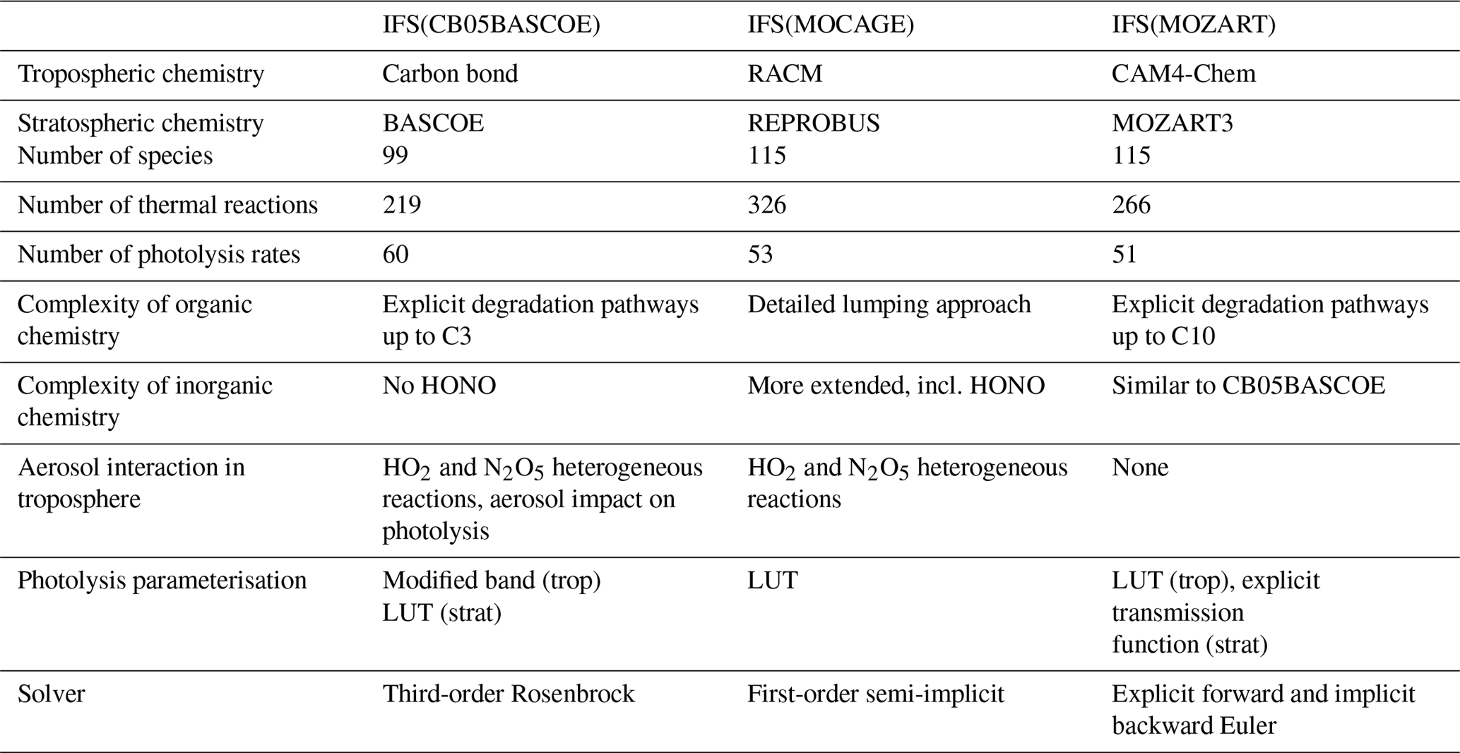
An overview of the most important differences in the three chemistry modules described above is given in Table 1. First, there are large differences in the choices made to compile the tropospheric chemistry mechanism. IFS(MOZART) describes the degradation of organic carbon types C1, C2, C3, C4, C5, C7 and C10, together with lumped aromatics, while IFS(CB05BASCOE) only describes explicit degradation up to C3, with the same reactions as present in IFS(MOZART). Instead, emissions and degradation of higher volatile organic compounds (VOCs) in IFS(CB05BASCOE) are lumped to a few tracers. Furthermore, the parameterisation of isoprene and terpene degradation is simpler in IFS(CB05BASCOE) than in IFS(MOZART). Aromatics are currently not described in IFS(CB05BASCOE), while they are accounted for with simple approaches in IFS(MOZART).
IFS(MOCAGE) describes many more lumped organic species than IFS(CB05BASCOE) and IFS(MOZART), also accounting for the more complex organics beyond C3. Furthermore, IFS(MOCAGE) uses a rather different lumping approach and contains more complexity for different terpene components, also including aromatics. Such differences are bound to impact the effective degradation of VOCs and thus ozone production efficiency and oxidation capacity (e.g. Sander et al., 2019).
With respect to the inorganic chemistry, the schemes are mostly similar. Still, IFS(MOCAGE) includes nitrous acid (HONO) chemistry, which is missing in both IFS(CB05BASCOE) and IFS(MOZART) implementations. Gas-phase sulfur chemistry is mostly similar between IFS(CB05BASCOE) and IFS(MOZART), while IFS(MOCAGE) has some more complexity by considering reactions involving dimethyl sulfoxide (DMSO) and H2S. Instead, IFS(CB05BASCOE) and IFS(MOZART) contain a treatment of gas–aerosol partitioning for nitrate and ammonium, which is missing in IFS(MOCAGE).
Significant uncertainty remains in the magnitude of heterogeneous reaction probabilities. Heterogeneous reactions of HO2 and N2O5 on aerosol are included in IFS(CB05BASCOE) and IFS(MOZART), although with different efficiencies, but not in the IFS(MOCAGE) version considered here. This has only become available in a more recent model version. Also, for instance, a more recent version of IFS(MOZ) with updated values following Emmons et al. (2010) leads to a significantly reduced NOx lifetime. So far, two-way coupling of secondary aerosol formation has not been available in any of the current model versions.
Regarding the treatment of photolysis in the troposphere, IFS(CB05BASCOE) applies a modified band approach, whereby for seven wavelengths the photolysis rates are computed online, taking into account the scattering and absorption properties of gases (overhead ozone and oxygen), clouds and aerosol. IFS(MOCAGE) adopts a lookup table approach, accounting for overhead ozone column, solar zenith angle, surface albedo and altitude, providing photolysis rates for clear-sky conditions. The impact of cloudiness on photolysis rates is applied online in IFS during the simulation using the parameterisation proposed by Brasseur et al. (1998). IFS(MOZART) applies the lookup table approach from MOZART-3 (Kinnison et al., 2007), considering overhead ozone column and cloud scattering effects on photolysis rates. Despite such larger differences, an intercomparison of an instantaneous field of photolysis rates showed similar average profiles, with a spread in magnitude in the range of 5 % in the tropical free troposphere for important photolysis rates like jO3, jNO2 and jHNO3. Locally, differences are larger and associated, amongst other factors, with different cloud treatment (Hall et al., 2018).
As for the stratospheric chemistry, IFS(CB05BASCOE) contains the largest complexity of the three model versions, with more species and reactions compared to the other mechanisms.
Different methods are used to solve the reaction mechanism. IFS(CB05BASCOE) applies the Rosenbrock solver, IFS(MOCAGE) here applies a first-order semi-implicit solver with fixed time steps, and IFS(MOZART) applies the explicit Euler method for species with long lifetimes (e.g. N2O) and an implicit backward Euler solver for other trace gases with short lifetimes. Experiments using different solvers for both IFS(CB05BASCOE) and IFS(MOCAGE) have revealed significant differences, with decreases in tropospheric ozone of the order of up to 20 % regionally when replacing a semi-implicit solver with the Rosenbrock solver. These differences are mostly traced to an increase in N2O5 chemical production (Cariolle et al., 2017), in turn reducing the NOx lifetime because of a larger net N2O5 loss on aerosol. This in turn leads to reduced chemical ozone production efficiency.
Table 1Specification of elemental aspects describing the three chemistry versions.
2.2 Emission, deposition and surface boundary conditions
The actual emission totals used in the simulation for 2011 from anthropogenic, biogenic and natural sources, biomass burning, and lightning NO are given in Table 2. MACCity emissions are used to prescribe the anthropogenic emissions (Granier et al., 2011), wherein wintertime CO traffic emissions have been scaled up according to Stein et al. (2014). Aircraft NO emissions are 1.8 Tg NO yr−1 , following Lamarque et al. (2010). Lightning NO emissions are parameterised as described in Flemming et al. (2015).
Monthly specific biogenic emissions originating from the MEGAN-MACC inventory (Sindelarova et al., 2014) are adopted, complemented with POET-based oceanic emissions (Granier et al., 2005).
Daily biomass burning emissions are taken from the Global Fire Assimilation System (GFAS) version 1.2, which is based on satellite retrievals of fire radiative power (Kaiser et al., 2012).
As described above, the chemistry mechanisms vary, particularly in their description of VOC degradation, with the most explicit treatment described in IFS(MOZ), while IFS(MOCAGE) and IFS(CB05BASCOE) rely on a more extended lumping approach. This has consequences for the partitioning of the various emissions. Still, we have ensured that the total of VOC and aromatic emissions in terms of tetragrams of carbon are essentially the same for the three chemistry schemes.
For CB05BASCOE, the emissions of “paraffins” (toluene and higher alkane emissions), “olefins” (butenes and higher alkenes) and “aldehydes” (acetaldehyde and other aldehydes) have been prescribed. Likewise, MOZART applies emissions of BIGALK (butanes and higher alkanes) and BIGENE (butenes and higher alkenes). MOCAGE adopts tracers HC3, HC5 and HC8, over which emissions of ethyne, propane, butanes and higher alkanes, esters, methanol, and other alcohols are distributed, whereas DIEN (butadiene) contains butenes and higher alkene emissions.
As for the aromatics, IFS(CB05BASCOE) disregards those, but includes toluene carbon emissions as part of the paraffins. IFS(MOZART) additionally treats a toluene tracer, while IFS(MOCAGE) contains two types of aromatics, designated TOL and XYL. These aromatic emissions are composed from toluene, trimethylbenzene, xylene and other aromatics.
Dry deposition velocities in the current configuration were provided as monthly mean values from a simulation using the approach discussed in Michou et al. (2004). To account for the diurnal variation in deposition velocities, a cosine function of the solar zenith angle is adopted with ±50 % variation. Wet scavenging, including in-cloud and below-cloud scavenging as well as re-evaporation, is treated following Jacob et al. (2000). The reader is referred to Flemming et al. (2015) for further details on dry and wet deposition parameterisation.
Methane (CH4), N2O and a selection of chlorofluorocarbons (CFCs) are prescribed at the surface as boundary conditions. While for N2O and CFC annually and zonally fixed values are currently assumed (Huijnen et al., 2016b), for CH4 zonally and seasonally varying surface concentrations are adopted based on a climatology derived from NOAA flask observations ranging from 2003 to 2014.
2.3 Model configuration and meteorology
The IFS model versions evaluated here were implemented in IFS cycle 43R1 and are run on a T255 horizontal resolution (∼0.7∘) with 60 model levels in the vertical up to 0.1 hPa, all excluding chemical data assimilation. The naming conventions and experiment IDs for the three model runs are specified in Table 3. For brevity we refer to the model runs as “CBA”, “MOC” and “MOZ”, respectively. A 30 min time stepping for the dynamics is applied, while meteorology is nudged towards ERA-Interim. To allow for sufficient model spin-up, the model versions are initialised for 1 July 2010 and run through until 1 January 2012. The initial condition (IC) fields have been generated for this date using fields that are as realistic and consistent as possible. For this purpose, tropospheric CO and O3 from the CAMS interim reanalysis (Flemming et al., 2017) have been combined with VOCs from its control run. CFCs, halogens and other tracers relevant for stratospheric composition originate from the BASCOE reanalysis v05.06 (Skachko et al., 2016) and have been merged for altitudes below the tropopause with model fields from Huijnen et al. (2016b), all specified for 1 July 2010. For MOZ and MOC, these IC fields have been completed for a few missing VOCs and CFCs using separate MOZART and MOCAGE climatologies, respectively. The first 6 months of the simulation are considered as spin-up and therefore not evaluated.
For the evaluation, the model was sampled in the troposphere and lower stratosphere (i.e. the lowest 40 model levels) every 3 h to have full coverage of the daily cycle. These are used to compute monthly to yearly averages. Standard deviations are computed to represent the model variability for a specified range in time and space.
3.1 Aircraft measurements
Aircraft measurements of trace gas composition from a database produced by Emmons et al. (2000) were used for the evaluation of distributions of collocated monthly mean modelled fields. Although these measurements cover only limited time periods, they provide valuable information about the vertical distribution of the analysed trace gases. The database is formed with data from a number of aircraft campaigns that took place during 1990–2001 which are gridded onto global maps, forming data composites of chemical species important for tropospheric ozone photochemistry. These are used to create observation-based climatologies (Emmons et al., 2000). Here we use measurements of ozone, CO, CH2O, C2H6, C2H4, methyl hydroperoxide (CH3OOH), NO2, nitric acid (HNO3) and sulfur dioxide (SO2). Note that the field campaigns used in this evaluation have been extended, also including data observed after the year 2000, such as the TOPSE and TRACE-P campaigns. The geographical distribution of the aircraft campaigns and their coverage areas are shown in Fig. 1.
Although the specific field campaign data are in theory representative for the specific year, the averaging of a large number of measurements over space and time partly solves the problem of interannual variability, and therefore these data can be considered as a climatology. Pozzer et al. (2009) showed that the correlation between model results and these observations would vary less than 5 % if model results 5 years apart were used. For the total anthropogenic VOC emissions the changes between the year 1990 and 2011 are of the order of 14 %, following the Emissions Database for Global Atmospheric Research (EDGARv4.3.2 database). Nevertheless, the evaluations presented here are all sampling background locations or outflow regions and are hence only partly affected by such changes in anthropogenic emissions. Also, the variability as well as measurement uncertainties present in the observations are larger than 14 %, implying that we can still consider these observations representative. Finally, these data summaries are useful for providing a picture of the global distributions of NMHCs and nitrogen-containing trace gases.
Table 2Specification of annual emission totals from anthropogenic, biogenic and natural sources, and biomass burning for 2011, in tetragrams of species mass, for three chemistry versions.

* Anthropogenic surface NO emissions (Tg NO) are split according to 90 % NO and 10 % NO2 emissions. Additionally, they contain a contribution of 1.8 Tg NO aircraft emissions and 9.2 Tg NO lightning emissions (LiNO).
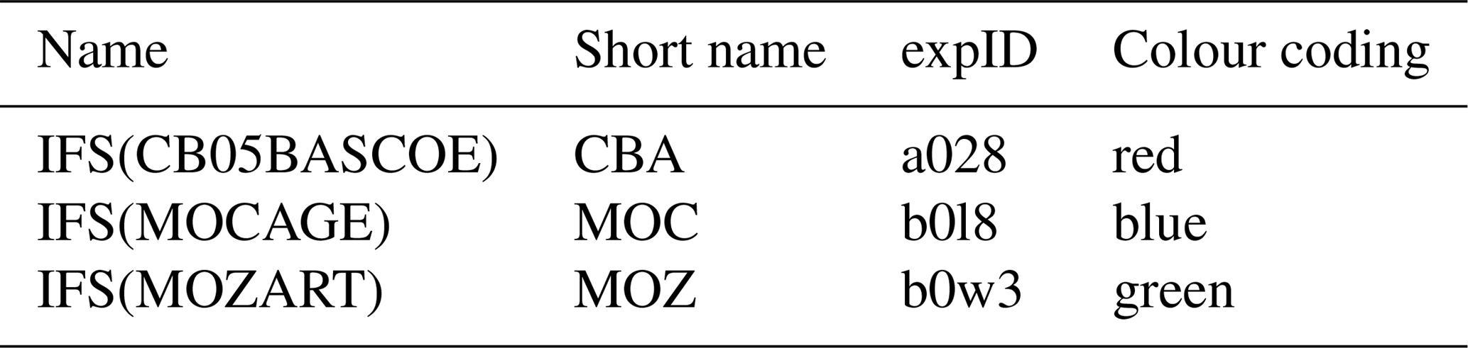
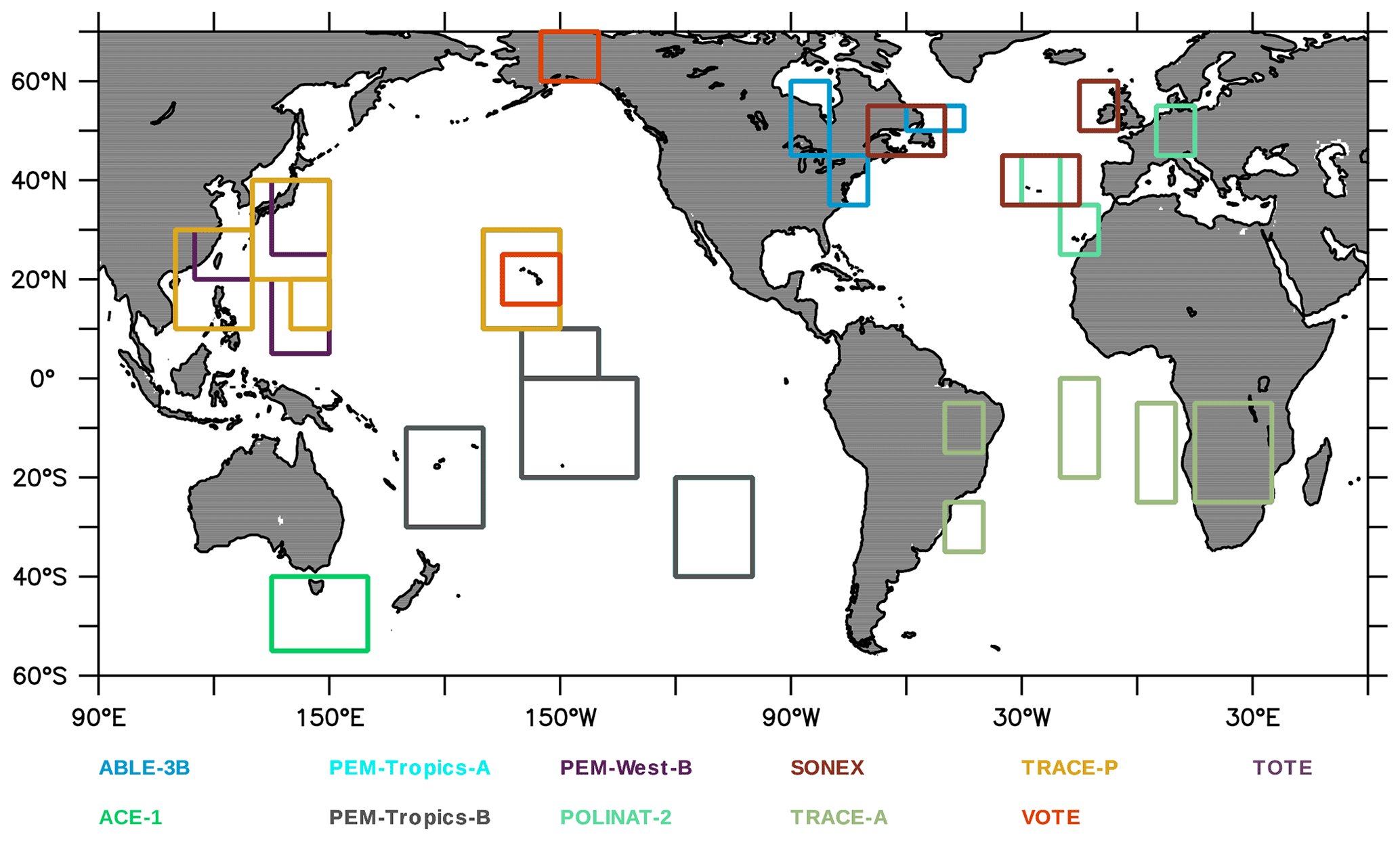
Figure 1Geographical distribution of the aircraft campaigns presented by Emmons et al. (2000). Each field campaign is represented by a different colour. Further information on the campaigns is found in Emmons et al. (2000).
3.2 Near-surface CO and ozone-sondes
In situ observations for monthly mean CO for the year 2011 are used to evaluate monthly mean modelled surface CO fields. Observational data are taken from the World Data Centre for Greenhouse Gases (WDCGG), the data repository and archive for greenhouse and related gases of the World Meteorological Organization (WMO) Global Atmosphere Watch (GAW) programme. The uncertainty of the CO observations is estimated to be of the order of 1–3 ppm (Novelli et al., 2003).
Tropospheric ozone was evaluated using sonde measurement data available from the World Ozone and Ultraviolet Radiation Data Center (WOUDC; http://woudc.org, last access: 25 April 2019), further expanded with observations from the Network for the Detection of Atmospheric Composition Change (NDACC) network. About 50 individual stations covering various worldwide regions are taken into account for the evaluation over the Arctic, Northern Hemisphere mid-latitudes, tropics, Southern Hemisphere mid-latitudes and the Antarctic. The 3-hourly output of the three model versions has been collocated to match the location and launch time of the individual sonde observations during 2011. The precision of ozone-sonde observations in the troposphere is of the order of −7 % to 17 % (Komhyr et al., 1995; Steinbrecht et al., 1998), while larger errors are found in the presence of steep gradients and where the ozone amount is low.

Figure 2Geographical distribution of the ozone-sondes during 2011 used for evaluation, coloured for the various seasons. The size of the triangles provides information on the relative number of observations available for each of the seasons and locations compared to the other locations. The geographical aggregation for the five latitude bands presented in Figs. 5 and 7, as well as the western Europe and eastern US regions, is also given.
3.3 Satellite observations
MOPITT (Measurements of Pollution in the Troposphere) v7 CO column observations (Deeter et al., 2017) are used to evaluate the CO total columns. The MOPITT instrument is a multi-channel thermal infrared (TIR) and near infrared (NIR) instrument operating onboard the Terra satellite. The total column CO product is based on the integral of the retrieved CO volume mixing ratio profile. A climatology based on CAM4-Chem (Lamarque et al., 2012) is used to provide the MOPITT a priori profiles. For our study we use the TIR-derived CO total column observations, which are provided over both the oceans and over land. The highest CO sensitivities of these MOPITT TIR measurements are in the middle troposphere at around 500 hPa. Sensitivity to the lower troposphere depends on the thermal contrast between the land and lower atmosphere, which is higher during the day than in the night. Therefore, in our study we only use daytime MOPITT TIR observations. The standard deviation of the error in individual pixels for the MOPITT v7 TIR product evaluated against NOAA flask measurements is reported as 0.13×10¹⁸ mol cm−2 (Deeter et al., 2017), i.e. of the order of 10 % of the observation value. Daily mean model CO columns have been gridded to a spatial resolution, and for our analysis we applied the MOPITT averaging kernels to the logarithm of the mixing ratio profiles, following Deeter et al. (2012).
OMI retrievals of tropospheric NO2 were taken from the QA4ECV dataset (Boersma et al., 2017). For this evaluation the 3-hourly model output of NO2 was interpolated in time to the local overpass of the satellite (13:30 h), while pixels with a satellite-observed radiance fraction originating from clouds greater than 50 % were filtered out. The averaging kernels of the retrievals are taken into account, hence making the evaluation independent of the a priori NO2 profiles used in the retrieval algorithm. Note that by using the averaging kernels the model levels in the free troposphere are given relatively greater weight in the column calculation, which means that errors in the shape of the NO2 profile can contribute to biases in the total column.
In this section we provide a basic assessment of the magnitude and differences in annual and zonal mean concentration fields between the three chemistry versions for a few essential tracers: O3, CO, NOx (NO + NO2) and OH. This provides a first insight into the correspondences and differences between chemistry modules and will help to interpret more quantitative differences seen in the evaluation against observations.
The annual zonal mean O3 mixing ratios (Fig. 2, top) show very similar patterns, with overall low values over the Southern Hemisphere (SH) and the highest over the Northern Hemisphere (NH) mid-latitudes, associated with the dominating emission patterns. Differences between chemistry versions are of the order of 10 %, with MOC comparatively showing the lowest values over the tropical free troposphere and MOZ the highest over the NH extratropics. Differences in tropospheric ozone between model versions are remarkably small on a global scale.
Likewise, annual zonal mean CO mixing ratios show the highest values associated with pollution regions in the tropics and over the NH. The highest values are obtained with CBA and the lowest with MOC, with differences ranging between 10 % and 20 %. As CO and precursor emissions are essentially identical, this is likely caused by differences in oxidising capacity, which is governed by OH abundance, as described below.
Zonal mean NOx mixing rations, a tracer playing a crucial role in ozone formation, show overall the highest values for MOC and the lowest for CBA. MOZ and CBA are overall similar, but MOC shows higher values in the lower and middle troposphere in the tropics and up to the NH high latitudes. This is likely related to the fact that in this version of IFS(MOCAGE) the coupling with the aerosol module has not yet been established, contrary to CBA and MOZ, implying a missing sink of NOx through the heterogeneous reaction of N2O5 to HNO3. Additionally, Cariolle et al. (2017) showed limitations of the semi-implicit method as used in MOC for resolving NOx chemistry. Both elements likely contribute to significantly larger tropospheric NOx lifetimes in MOC compared to CBA and MOZ. In contrast, the NOx lifetime in the IFS(CB05BASCOE) scheme is comparatively short, which is associated with a diagnosed relatively efficient organic nitrate production term from the reaction of NOx with VOCs in the modified CB05 mechanism compared to other mechanisms, as assessed in a box-modelling configuration (Sander et al., 2019).
Figure 2 also shows the annual zonal mean concentrations of OH. Overall, the magnitude of OH is largest for MOC and lowest for CBA, with MOZ in between. The largest differences in absolute terms are found in the tropics, where the concentrations are highest. Nevertheless, in relative terms the largest differences are found in the extratropics, particularly over the SH, as can be seen from Fig. 3. This figure shows the temporal evolution of the difference between MOC and MOZ simulated daily average OH at 600 hPa. This shows that differences can be up to 50 % in daily averages, in particular over the extratropics where the absolute values are lower compared to those in the tropics.
Tropospheric NOx in MOC is comparatively high, suggesting relatively efficient O3 and OH production. On the other hand, the photolysis rates of tropospheric ozone, responsible for the primary production of OH, are very similar (not shown). Therefore, the ozone production in MOC must be counter-balanced by a relatively large loss through reaction with OH and HO2 (which are the other major loss terms in the ozone cycle), suggesting a relatively short tropospheric O3 lifetime. An assessment of the ozone chemical production and loss terms is beyond the scope of this work. But such differences in oxidation capacity naturally have important implications for understanding differences in the performance of NMHCs, as discussed in the next sections.
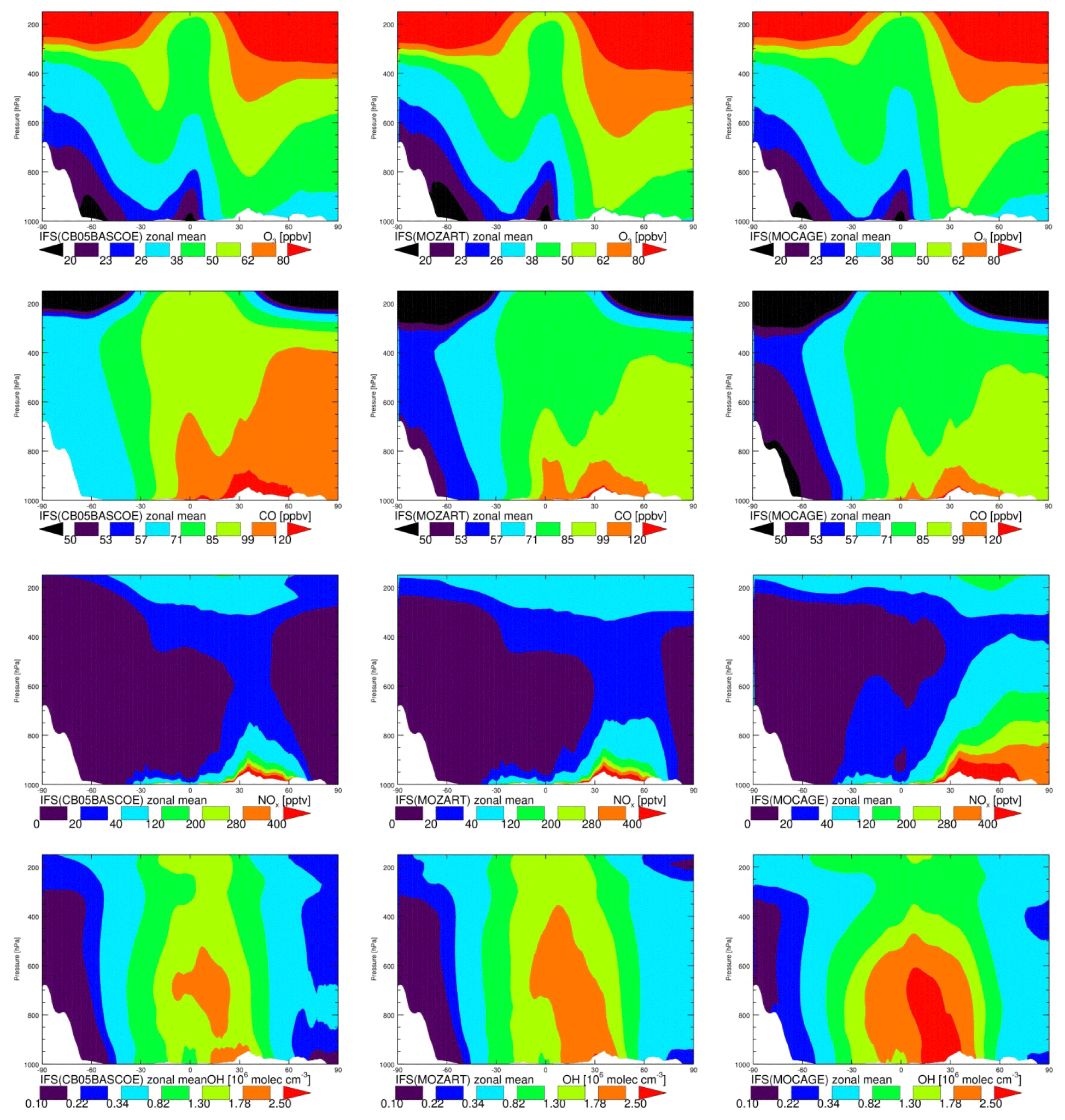
Figure 3Zonal annual mean O3, CO, NOx, mixing ratios and OH concentrations in CBA (a), MOZ (b) and MOC (c).
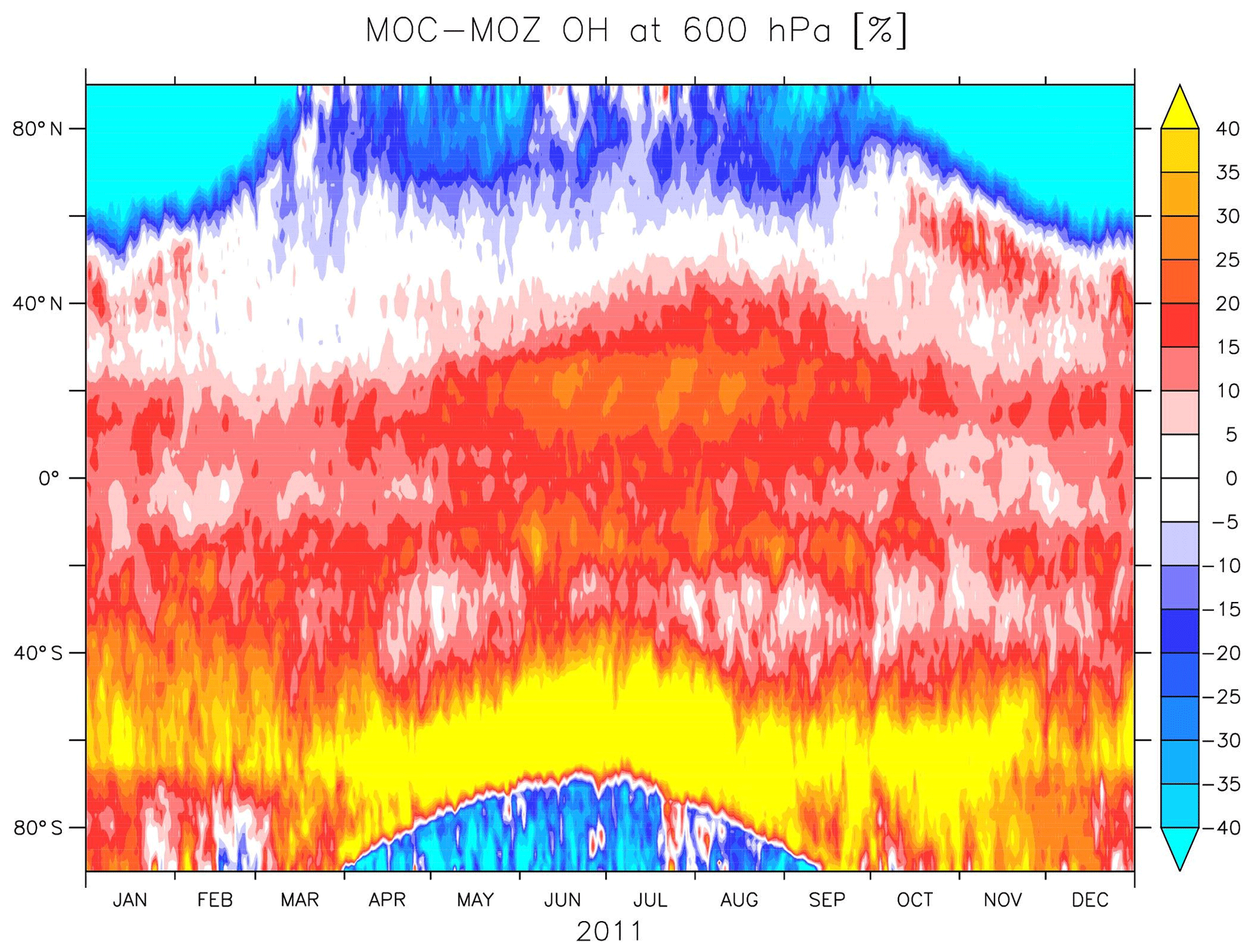
Figure 4Relative differences (in percent) of OH daily averaged mixing ratios of simulation MOC with respect to MOZ at 600 hPa.
In this section we evaluate the model simulations against a range of observations, including ozone-sondes, aircraft measurements and satellite observations, for carbon monoxide and nitrogen dioxide.
Table 4 summarises the comparison of the various model results with aircraft measurements described in Sect. 3.1 in terms of biases and correlation, in terms of explained variance (R2), both unweighted and weighted with uncertainties, which are approximated by the root mean square of model variability and measurement variability. Here model variability is represented by the standard deviation from the averaged output values, and measurement variability is represented by the combination of instrumental errors and standard deviation. As explained in further detail by Jöckel et al. (2006), with this approach, the measurement locations with high variability have less weight, whereas more weight is given to stable, homogeneous conditions. This allows us to compare values that are more representative for the average conditions and to eliminate specific episodes that cannot be expected to be reproduced by the model. For this reason the weighted correlations are also generally expected to be higher than the normal correlations.
Also according to this analysis, the discrepancies between model results and measurements are smaller than the uncertainties if the absolute value of the weighted bias (i.e. in units of the normalised standard deviation, Table 4) for a specific tracer is less than 1. A high weighted correlation in combination with a weighted bias of [] indicates that the model is able to reproduce the observed mixing ratios on average. This holds for all versions for CO, O3, CH2O, NO2 and HNO3, while model versions have more difficulties with CH3OOH. For SO2 CBA is the only model version to deliver a weighted bias that is larger than −1. For C2H4 and C2H6 none of the versions are able to match the observations to an acceptable degree. Remarkably, C2H4 is the only trace gas for which values for the weighted R2 are lower than the normal R2 values, suggesting fundamental problems representing this trace gas properly in any of the chemistry versions. The inability of the model versions to reproduce the observed magnitude of C2H6 and the vertical distribution of C2H4, as indicated by the relatively low correlation with all aircraft measurements included in the database, requires a more detailed analysis. This is investigated in more detail in the next sections.
Table 4Summary of the bias and correlation coefficients (in terms of explained variance, R2) of model results versus all available aircraft observations, also weighted with relative uncertainties. Bias: model results minus observations.
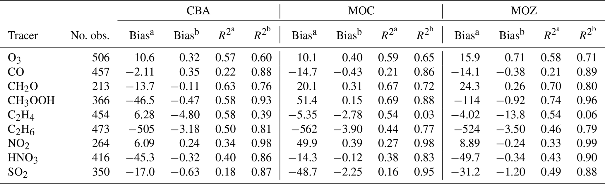
a Bias is given in pmol mol−1 (nmol mol−1 for CO and O3). b Bias is in standard deviation units. Likewise, is the normal correlation coefficient, and is the correlation coefficient weighted with standard deviations (see text).
5.1 Ozone (O3)
Figure 4 compares tropospheric O3 profiles simulated by the three model versions with ozone-sonde observations for six different regions over the four seasons. Overall the three chemistry versions deliver a similar performance, reproducing the regionally averaged variability in O3 observations, with various biases depending on the season, region and altitude range. Typically, the model versions tend to simulate lower O3 mixing ratios in the SH middle and high latitudes compared to sonde observations and higher in the tropics. Over the Arctic, western Europe, the eastern US and the tropics, MOZ simulates too-high O3 concentrations at all altitudes and for all seasons except June–July–August (JJA), with average positive biases ranging from 1 to 12 ppbv in the free troposphere. Here it is worth mentioning that recent updates to reaction probabilities and aerosol radius assumptions in the heterogeneous chemistry module in IFS(MOZART) significantly improved O3 concentrations, particularly in the NH.
MOC shows positive biases over the NH mid-latitudes during winter and spring and negative biases during Arctic winter in the lower troposphere (< 700 hPa) as well as in the 700–300 hPa range in summer. CBA simulates O3 mixing ratios that are generally in close agreement with observations over the Arctic and NH mid-latitudes, but negative biases up to 10 ppbv are obtained in the Arctic upper troposphere (500–300 hPa) during wintertime (Fig. 5, top panel). All three model versions are consistently too high close to the surface (> 800 hPa) over the tropics for all seasons, but particularly during December–January–February (DJF). Over the Antarctic and, to a lesser extent, the SH mid-latitudes all three model versions underestimate O3, with negative biases up to 10 ppbv for a large part of the year. However, it should be noted that in the SH regions this evaluation is less representative because there are very few observations.
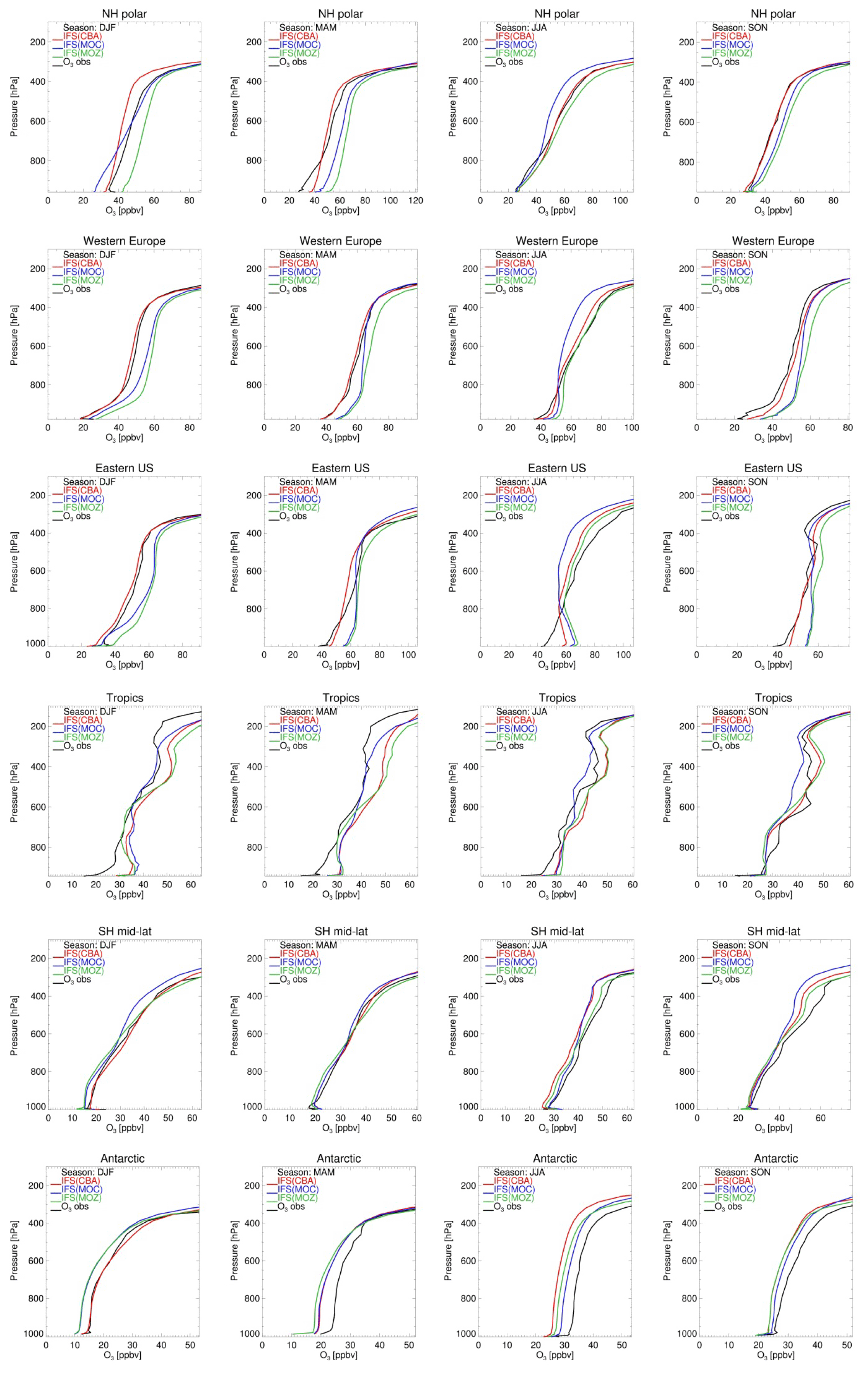
Figure 5Tropospheric ozone profiles from model versions CBA (red), MOC (blue) and MOZ (green) against sondes (black) in volume mixing ratios (ppbv) over six different regions (from top row to bottom row): NH polar (90–60∘ N), western Europe (45–54∘ N; 0–23∘ E), eastern US (32–45∘ N; 90–65∘ W), the tropics (30∘ N–30∘ S), SH mid-latitudes (30–60∘ S) and the Antarctic (60–90∘ S), averaged over four seasons (from left to right: December–January–February, March–April–May, June–July–August, September–October–November).

Figure 6Mean tropospheric ozone profiles from model versions CBA (red), MOC (blue) and MOZ (green) against sondes (black) in volume mixing ratios (ppbv) during DJF and JJA at selected individual stations. Error bars represent the 1σ spread in the seasonal mean observations.
Figure 5 shows an evaluation of O3 profiles against sondes at selected individual WOUDC sites representative of the Arctic (Ny-Ålesund), NH mid-latitudes (Lindenberg), the tropics (Hong Kong, Nairobi), SH mid-latitudes (Lauder) and the Antarctic (Neumayer) for DJF and JJA seasons in 2011. We note generally similar biases compared to those for the regional averages, even though local conditions play a larger role in explaining the different performance statistics for these stations. Overall, the evaluation at individual stations provides reasonable agreement between model simulations and sondes.
Evaluation against the aircraft climatology as provided in Table 4 shows on average a positive bias in the range of 10 (CBA and MOC) to 16 ppbv (MOZ), while the correlation statistics show generally acceptable values (R2>0.57), giving overall confidence in the model ability to describe ozone variability. Figure 6 shows annually averaged model biases and root mean square errors (RMSEs) for various latitude bands and for altitude ranges 900–700, 700–500 and 500–300 hPa against WOUDC sondes. In this evaluation we also present data from the CAMS interim reanalysis (CAMSiRA) for the year 2011 to put the current model evaluation into perspective. This summary analysis shows averaged biases within ±10 ppbv, which is also in line with the O3 bias statistics against the aircraft climatology. At lower altitudes the model biases are mostly equal to or better than those from CAMSiRA, while above 500 hPa CAMSiRA delivers mostly smaller biases thanks to the assimilation of satellite ozone observations. The RMSE shows a larger spread in the lower troposphere of the NH, while at higher altitudes above 500 hPa the overall magnitude of the RMSE for the three chemistry versions converges to values ranging from 10 to 16 ppbv, depending on the latitude. Here CAMSiRA shows overall better performance, mainly for the tropics and SH, while over the NH its performance is similar to IFS(CBA). This evaluation summarises common discrepancies between model versions and observations, such as the negative bias over the Antarctic and positive bias below 700 hPa for tropical stations (see also Fig. 4), suggesting biases in common parameterisations such as transport, emissions and deposition. The largest discrepancies between model versions have been detected at northern middle and high latitudes below 500 hPa, with significantly higher values for RMSE for MOC and MOZ compared to CBA. A comparatively large positive bias for MOZ was detected, which has been linked to an underestimate of the N2O5 heterogeneous loss efficiency. The differences between MOC and CBA can likely be explained by similar aspects that are likely as important to explain differences with respect to the performance of IFS(MOCAGE).
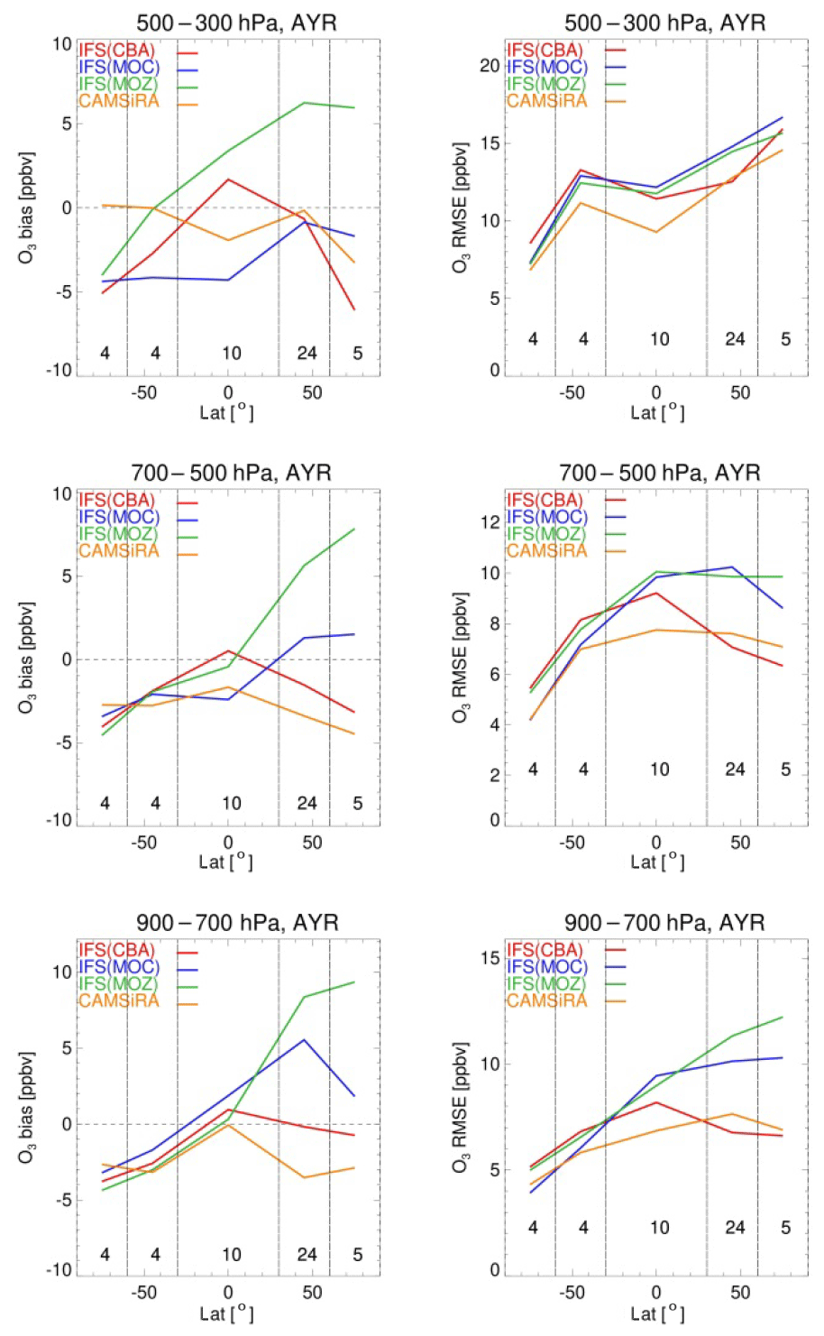
Figure 7Mean of all model biases (a) and RMSE (b) values against ozone-sondes as a function of latitude for various pressure ranges (top row: 300–500; middle row: 500–700; bottom row: 700–900 hPa), averaged over the full year. Same colour codes as in the previous figure. The numbers in each latitude range indicate the number of stations that contribute to these statistics. For reference, the corresponding results from the CAMS interim reanalysis (CAMSiRA) are also given in orange.
5.2 Carbon monoxide (CO)
Carbon monoxide is a key tracer for tropospheric chemistry, as a marker of biomass burning and anthropogenic pollution, and provides the most important sink for OH. Approximately half of the CO burden is directly emitted, and the rest is formed through degradation of CH4 and other VOCs (Hooghiemstra et al., 2011). Hence, a correct simulation of this tracer is very important for studies of atmospheric oxidants. Considering the use of the same emissions and CH4 surface conditions, differences in CO concentrations are essentially caused by differences in chemistry.
Figures 7 and 8 show the monthly mean evaluation against MOPITT total CO columns for April and August 2011. Whereas generally the model versions show good agreement with the observations in terms of their spatial patterns, persistent seasonal biases remain, such as the negative bias over the NH during April (further analysed in, e.g. Shindell et al., 2006; Stein et al., 2014) and a negative bias over Eurasia during August. For all three chemistry versions the patterns of enhanced CO in the tropics, associated with biomass burning, are generally well captured, as is the magnitude of CO columns over the SH. Looking at differences between model versions, CBA shows the overall highest magnitudes, implying a smaller negative bias over the NH, particularly during April, while this simultaneously results in an emerging positive bias in the tropics.
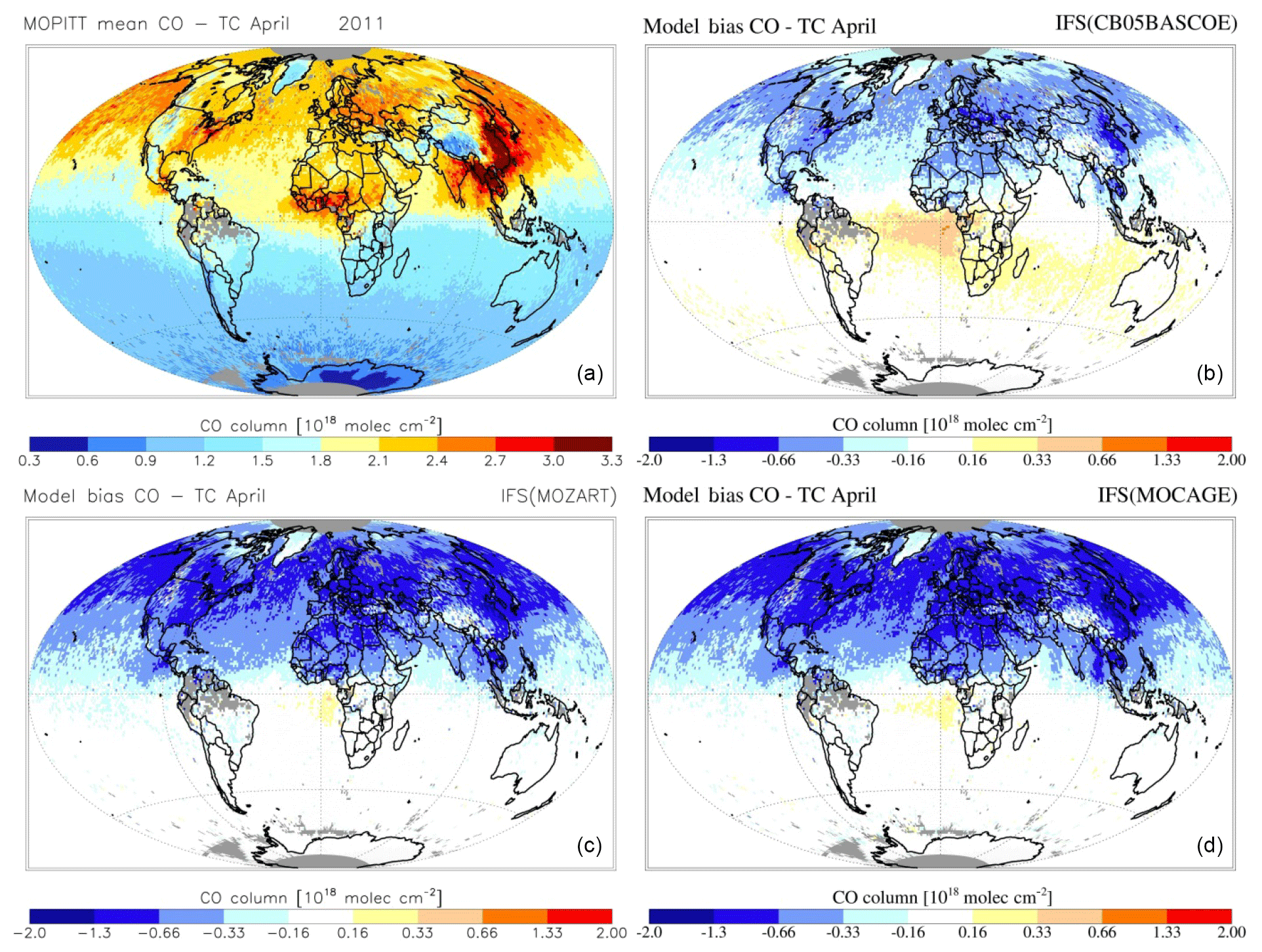
Figure 8MOPITT CO total column retrieval for April 2011 (a) and simulated by IFS(CBA) (b), IFS(MOZ) (c) and IFS(MOC) (d).
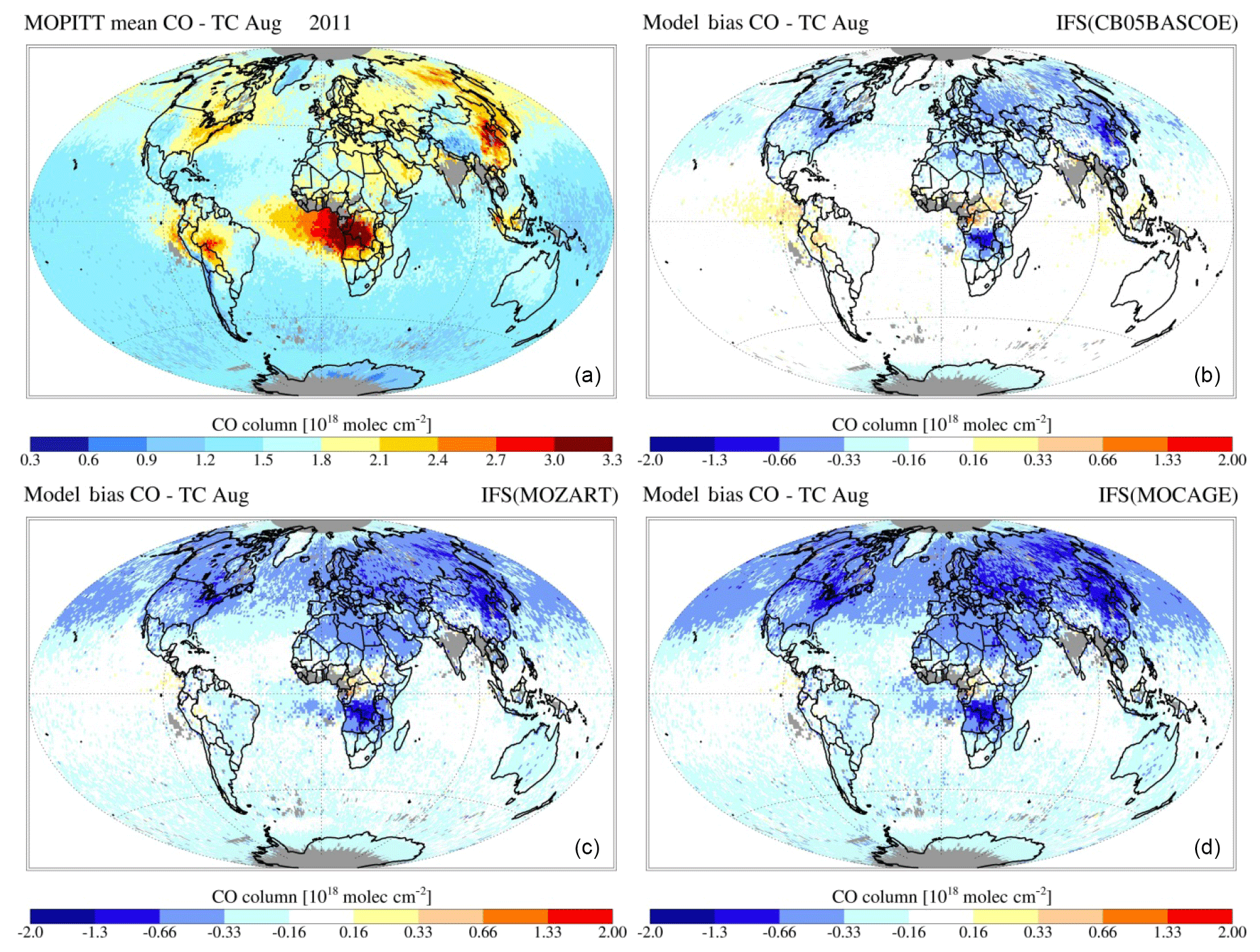
Figure 9MOPITT CO total column retrieval for August 2011 (a) and simulated by IFS(CBA) (b), IFS(MOZ) (c) and IFS(MOC) (d).
In Fig. 9 the annual cycle at selected GAW stations is shown, while Fig. 10 additionally shows the corresponding temporal correlation between the simulated monthly mean CO for all stations. Even though the phase and amplitude of the annual cycle are well reproduced by the model versions at several locations (e.g. Mauna Loa, Hawaii), the concentrations tend to be overestimated in the Southern Hemisphere, particularly by CBA and to a lesser extent by the other chemistry versions, and underestimated over the remote Northern Hemisphere. This points to sensitivities due to the applied chemistry scheme mainly associated with differences in OH, which is lowest in CBA and highest in MOC (see also Sect. 4). A possible overestimation of CO over the tropics and Southern Hemisphere could relate to uncertainties in the biogenic emissions (Sindelarova et al., 2014).
The correlations (in terms of R2) of monthly mean time series against GAW stations are mostly above 0.8. Particularly over Antarctica, the correlation is very high with R2≈0.9, indicating that the main processes controlling the CO abundance are indeed well represented by the model. Nevertheless, at locations between 40 and 60∘ N the correlation is lower. These regions are strongly influenced by local chemistry and emissions, including industry and biomass burning. Clearly, the seasonal cycle is not optimally reproduced in northern America (Canada regions) by any of the three chemistry versions, indicating that uncertainties in regional emissions, such as boreal biomass burning, could be responsible for these disagreements.

Figure 10Comparison of CO mixing ratios (ppbv) at the surface as simulated (red, blue and green are model results from CBA, MOC and MOZ, respectively) and observed (black) at 12 stations sorted by decreasing latitudes. The bars represent 1 standard deviation of the monthly average for the location of the station.

Figure 11Temporal correlation (R2) between monthly mean surface CO as derived from observations (GAW network) and model simulations (a: CBA, b: MOC, c: MOZ).
Compared to aircraft observations (see Fig. 11), the three model versions produce similar CO mixing ratio vertical profiles, with differences among them typically within the range of 10 %–20 %, depending on the location. The biomass burning plumes are reproduced consistently (see Fig. 11, TRACE-A, West Africa coast), and all three models compare well with observations for both background conditions in the Northern Hemisphere (SONEX, Ireland) and highly polluted conditions (PEM-West-B, China coast).
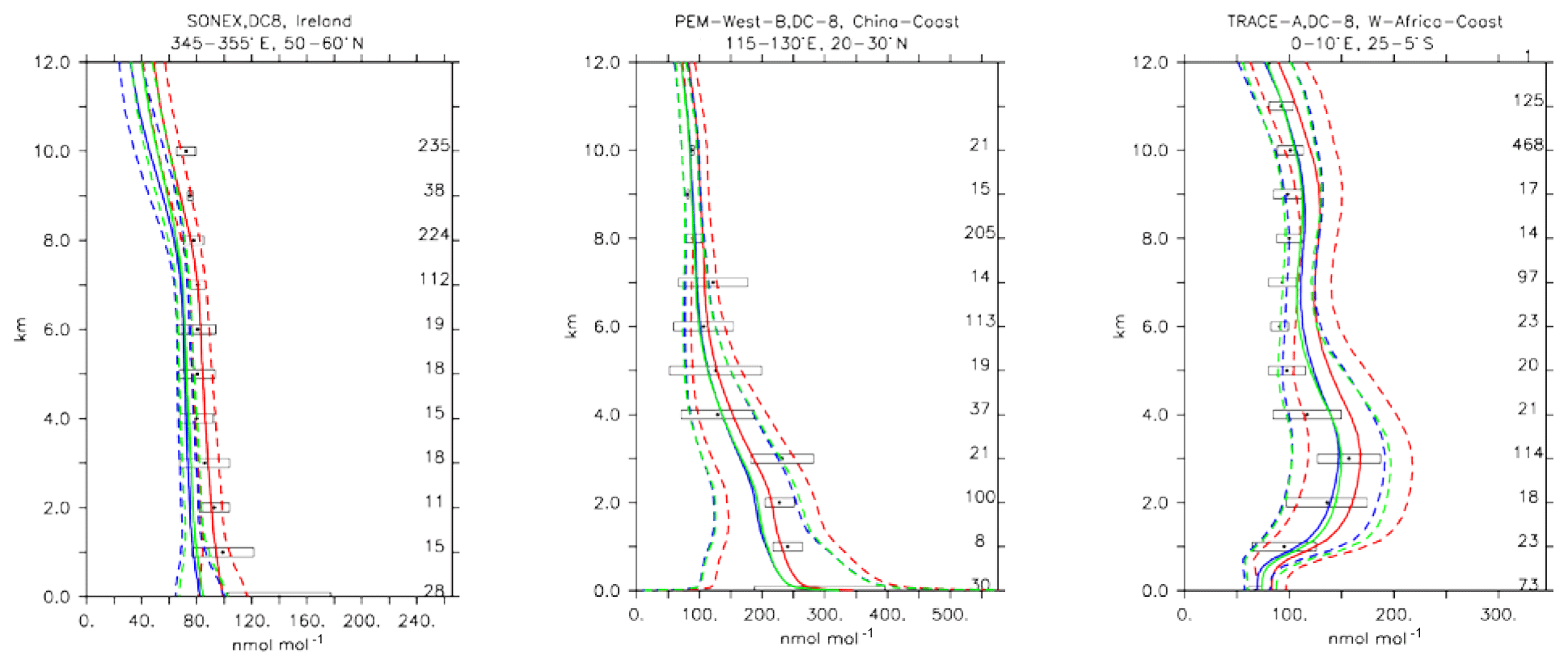
Figure 12Comparison of simulated CO vertical profiles by using the CBA (red solid line), MOC (blue solid line) and MOZ (green solid line) chemistry versions against aircraft data (black dots). Also shown are the modelled (dashed lines) and measured (black rectangular) standard deviations. The numbers on the right vertical axis indicate the number of available measurements.
5.3 Formaldehyde (CH2O) and methyl hydroperoxide (CH3OOH)
Formaldehyde is important as one of the most ubiquitous carbonyl compounds in the atmosphere (Fortems-Cheiney et al., 2012). It is mainly formed through the oxidation of methane, isoprene and other VOCs such as methanol (Jacob et al., 2005), while its oxidation and photolysis are responsible for about half of the CO in the atmosphere. A good agreement of the simulations with the observations can be seen from Fig. 12, where the vertical profile from selected aircraft observations and model simulations is shown. Also from Table 4 it is clear that all three model versions reproduce formaldehyde accurately. The weighted bias is always well below 1 standard deviation unit (i.e. −0.11, 0.31 and 0.26 for CBA, MOC and MOZ, respectively), indicating that the simulations are well within the statistical uncertainties.
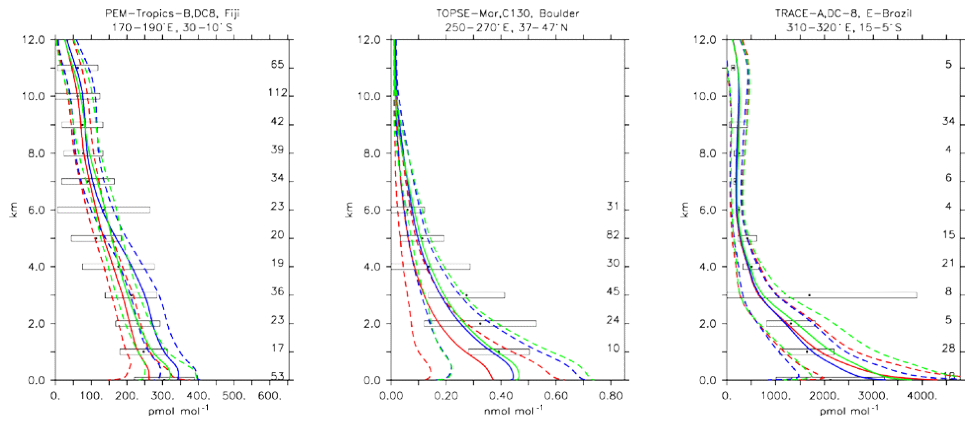
Figure 13Comparison of simulated CH2O vertical profiles by using the CBA (red), MOC (blue) and MOZ (green) chemistry versions against aircraft data (black). Line styles and symbols have the same meaning as in Fig. 12.
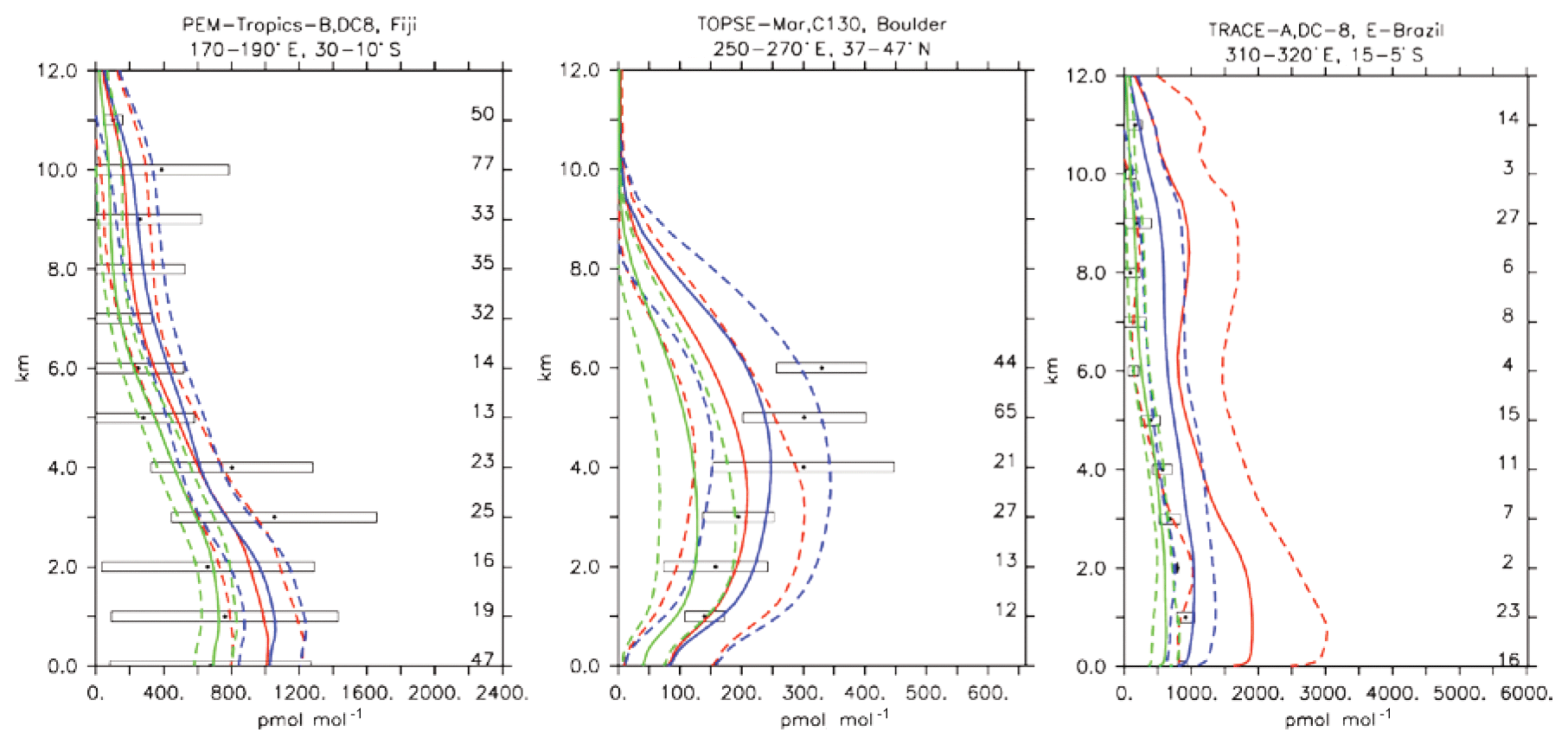
Figure 14Comparison of simulated CH3OOH vertical profiles by using the CBA (red), MOC (blue) and MOZ (green) chemistry versions against aircraft data (black). Line styles and symbols have the same meaning as in Fig. 11.
CH3OOH is a main organic peroxide acting as a temporary reservoir of oxidising radicals (Zhang et al., 2012). It is mainly formed through reaction of CH3O2+HO2, which are both produced in the oxidation process of many hydrocarbons. The CH3OOH lifetime of about 1 d globally is mainly governed by its reaction with OH and photolysis. Figure 13 presents an evaluation for CH3OOH for the same sites presented for CH2O in Fig. 12. Mixing ratios are generally reasonably within the range of the observations, for example over the tropical Pacific over Fiji. A larger spread between model versions, with a strong overestimate for CBA, is found in the Amazon region over Brazil. As a global average, a comparatively large underestimate for MOZ and, to a lesser extent, also for CBA was found; see also Table 4. Nevertheless, correlations, especially those weighted with the uncertainties, are overall good, giving general confidence in the modelling.
Considering the short lifetimes for CH2O (a few hours in daytime) and also CH3OOH, as well as the large dependence of their abundances on details of the VOC degradation scheme, which vary across the chemistry versions presented here, it is beyond the scope of this paper to explain these differences. This would require a detailed assessment of the respective production and loss budgets, which are currently not available.
5.4 Ethene (C2H4)
Ethene is the smallest alkene which is primarily emitted from biogenic sources. In our configuration, biogenic C2H4 emissions are 30 Tg yr−1, which appears at the upper end of such emission estimates as reported by Toon et al. (2018). The rest of the emissions are attributed to incomplete combustion from biomass burning or anthropogenic sources.
The three chemical mechanisms produce mostly very similar mixing ratios of C2H4. Nevertheless, as indicated by the bias (Table 4), which ranges between −2 and −14 in standard deviation units, as well as the weighted correlations, the model versions have difficulties in simulating C2H4. Even though this evaluation should only be considered in a climatological sense, the vertical profiles (see Fig. 13) are strongly biased (e.g. SONEX, Newfoundland and PEM-Tropics-A, Tahiti), with positive biases occurring at the surface and negative biases in the free troposphere. In remote regions and at higher altitudes, where the direct influence of emissions is lower, the model is at the lower end of the range of observations, with frequent underestimates (see Fig. 13, PEM-Tropics-A, Christmas Island). This was already observed in other studies (e.g. Pozzer et al., 2007), implying that the chemistry of this tracer is not well understood. As the underestimation appears to be ubiquitously distributed, this suggests that C2H4 decomposition is too strong or that the model versions miss some chemical production terms (e.g. Sander et al., 2019).
Furthermore, it is interesting to note the comparatively large difference present between the simulations at high latitudes (e.g. SONEX, Newfoundland), where the largest relative differences in modelled OH have been found (see also Sect. 4), illustrating the importance of OH for explaining inter-model differences. CBA indeed shows the largest values for C2H4, which is explained by the comparatively low abundance of OH in this model version.
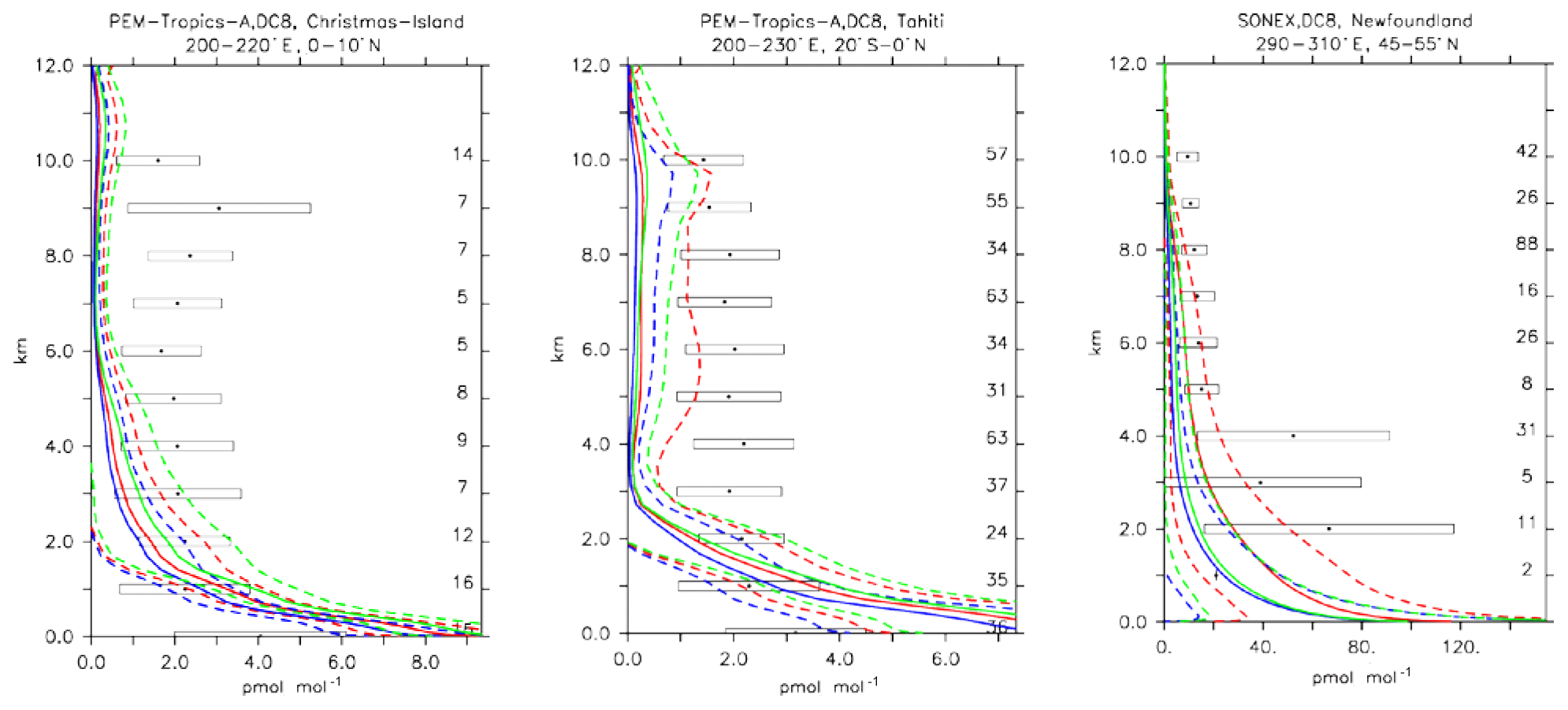
Figure 15Comparison of simulated C2H4 vertical profiles by using the CBA (red), MOC (blue) and MOZ (green) chemistry versions against aircraft data (black). Line styles and symbols have the same meaning as in Fig. 12.
5.5 Ethane (C2H6)
Ethane (C2H6) is the lightest trace gas of the family of alkanes and has an atmospheric lifetime of about 2 months. Ethane emissions are primarily of anthropogenic nature and have seen a relatively strong decrease since the 1980s (Aydin et al., 2011). Nevertheless, since 2009 an increase in C2H6 concentrations has been observed, believed to be associated with recent increases in CH4 fossil fuel extraction activities (Hausmann et al., 2016; Monks et al., 2018).
Compared to aircraft observations, all three model versions significantly underestimate the C2H6 observed mixing ratios at all locations and ubiquitously (see Fig. 14). A particularly strong underestimation is found in the Northern Hemisphere, where most of the observations are located (e.g. the SONEX campaign over Ireland). A strong negative bias was also reported in the overall statistics (Table 4), even though, contrarily to C2H4, the weighted correlation showed acceptable values for all versions (R2>0.7). These findings can be explained well by an underestimation of the MACCity-based C2H6 emissions, which are at least a factor of 2 lower than the corresponding estimates of 12–17 Tg yr−1 reported in the literature (Monks et al., 2018; Aydin et al., 2011; Emmons et al., 2015; Folberth et al., 2006). On the other hand, the comparison with the TRACE-A field campaign, which covered long-range transport of biomass burning plumes, shows a reasonable agreement in the lower troposphere (1–4 km), i.e. at the location of the biomass plume, suggesting appropriate biomass burning emissions. Still, a considerable underestimation is present in the upper troposphere, probably due to the missing background concentration.

Figure 16Comparison of simulated C2H6 vertical profiles by using the CBA (red), MOC (blue) and MOZ (green) chemistry versions against aircraft data (black). Line styles and symbols have the same meaning as in Fig. 12.
5.6 Nitrogen dioxide (NO2)
Nitrogen dioxide is a trace gas difficult to compare with in situ observations due to its photochemical balance with nitric oxide. Nitrogen dioxide shows a strong diurnal cycle, mainly due to the fast photolysis rate. Here only daytime values have been used to construct the model averages because the observations from the various field campaigns were equally conducted in daylight conditions. Figure 15 shows the strong variability in daytime NO2 values in both the measurements and the simulations. In general the MOC simulation shows the highest concentration of NO2 in different locations, particularly over source regions (see Fig. 15; TRACE-P, Japan, and TOPSE-Feb, Boulder), with MOZ and CBA being more similar. This is in line with the analysis given in Sect. 4. Outside the source regions the secondary processes (such as its equilibrium with HNO3; see also next section) have larger influences, and hence the model and observation profiles of NO2 show even stronger variability and larger differences (see Fig. 15; TOPSE-May, Thule). Still, in general all the chemical mechanisms are able to reproduce NO2 within 1 standard deviation (see Table 4), even though the unweighted mean bias for MOC is significantly higher than for CBA and MOZ.
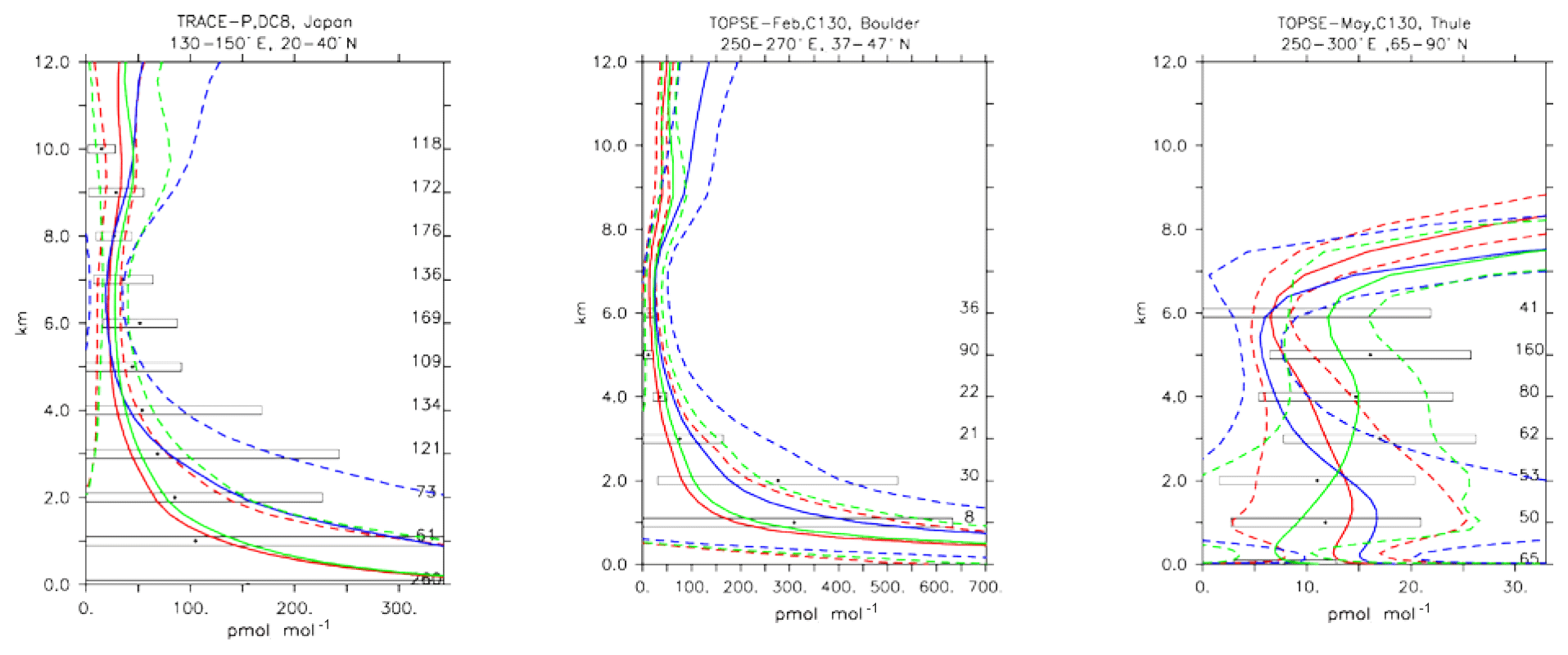
Figure 17Comparison of daytime NO2 vertical profiles simulated by CBA (red), MOC (blue) and MOZ (green) chemistry versions against aircraft data (black). Line styles and symbols have the same meaning as in Fig. 12.
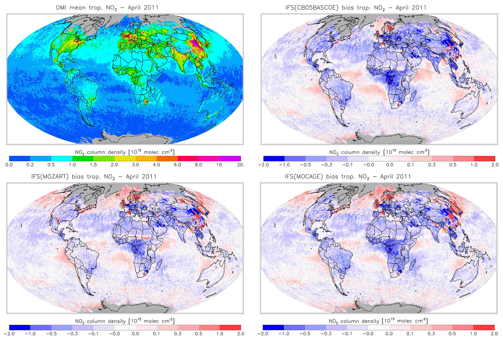
Figure 18Monthly mean tropospheric NO2 columns from OMI satellite retrievals from the QA4ECV product for April 2011, along with the corresponding collocated model biases.
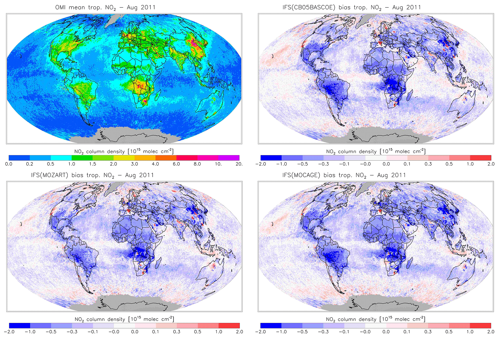
Figure 19Monthly mean tropospheric NO2 columns from OMI satellite retrievals from the QA4ECV product for August 2011, along with the corresponding collocated model biases.
Figures 16 and 17 evaluate tropospheric NO2 using the OMI satellite observations. The simulations deliver generally appropriate distributions with a correct extent of the regions with high pollution, as largely dictated by the emission patterns. Nevertheless, a general underestimation of NO2 over West Africa in April and Central Africa and South America in August is found, suggesting uncertainties associated with the modelling of biomass burning emissions.
Another interesting finding is a relatively strong negative bias over the Eurasian and North American continents in April for CBA, which is stronger than modelled in MOZ and MOC. In contrast, MOC in particular (but also MOZ) overestimates NO2 over the comparatively clean North Atlantic and North Pacific oceans in April. This all suggests a relatively short NOx lifetime in CBA compared to MOZ and MOC, which in turn helps to explain the lower O3 over the NH mid-latitude regions as modelled with CBA (see Fig. 5). The causes of these differences in modelled NO2 are mainly the use of a different numerical solver and differences in the efficiency assumed for N2O5 heterogeneous reactions (see Sect. 2.1.4). In August the differences in tropospheric NO2 between the three model versions are smaller than in April.
5.7 Nitric acid (HNO3)
Compared to several of the trace gases previously analysed, nitric acid is not primary emitted but is purely photochemically formed in the atmosphere. It has a very high solubility and therefore tends to be scavenged by precipitation very efficiently, providing an effective sink for the NOx family. Furthermore, it can act as a precursor for nitrate aerosols (Bian et al., 2017). HNO3 concentrations are therefore expected to show the largest variation between the simulations, as the production and sink terms can largely differ due to uncertainties in the parameterisations. In Fig. 18, the model results are compared with selected aircraft measurements. Although all three models tend to reproduce HNO3 in a statistically similar way, over the lower troposphere and up to 2 km of height MOC tends to result in higher HNO3 concentrations compared to the other two chemical mechanisms and measurements. This is also reflected by the overall lowest negative biases in Table 4. While MOC performs better at higher altitudes, in a biomass burning plume (e.g. TRACE-A; Fig. 18), it also overestimates the production of HNO3 or underestimates its sinks. Over polluted regions (Fig. 18; TRACE-P, Japan), all models tend to perform well, but in remote areas (Fig. 18; TOPSE, Churchill) the discrepancies between the models increase, with MOC delivering twice as much HNO3 as the other two model versions. Nevertheless, as the variability of the observations is very large, all the model versions still fall within the range of uncertainties of the observations. The discrepancies between the model versions can be mainly attributed to differences in NOx lifetimes, associated with differences in heterogeneous chemistry, and parameterisations for nitrate aerosol formation, as discussed in Sect. 2.1.4.
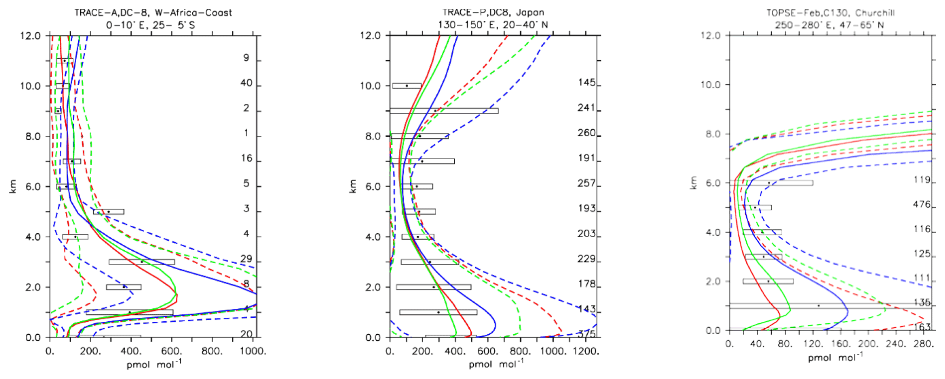
Figure 20Comparison of simulated HNO3 vertical profiles by using the CBA (red), MOC (blue) and MOZ (green) chemistry versions against aircraft data (black). Line styles and symbols have the same meaning as in Fig. 12.
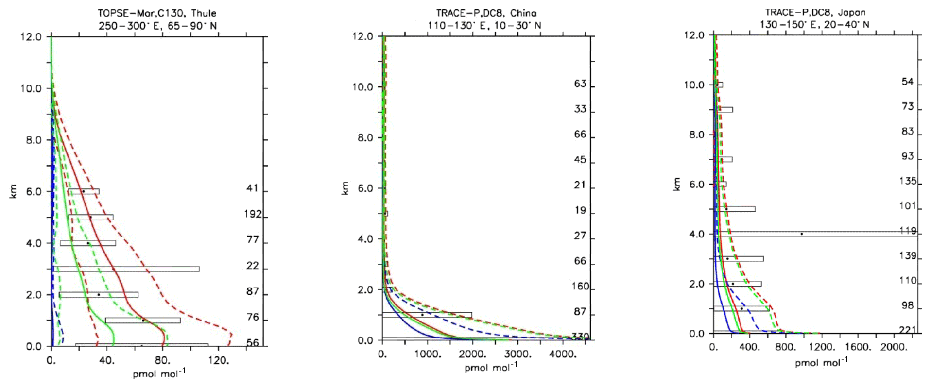
Figure 21Comparison of simulated SO2 vertical profiles by using the CBA (red), MOC (blue) and MOZ (green) chemistry versions against aircraft data (black). Line styles and symbols have the same meaning as in Fig. 12.
5.8 Sulfur dioxide (SO2)
Similar to HNO3, SO2 is also strongly influenced by wet deposition due to its high solubility. Furthermore, SO2 is primarily emitted and converted to sulfuric acid (H2SO4) both by gas-phase and aqueous-phase oxidation, an essential process for the production of new sulfate aerosol particles. Considering the complexity of the processes that control the SO2 fate in the atmosphere, large variability is expected for this tracer. The evaluation of SO2 shows that among the three chemistry versions, CBA always produces the highest SO2 mixing ratios, whereas MOC produces the lowest, and MOZ always lies in between. Nevertheless, all three mechanisms tend to underpredict SO2 mixing ratios (see Table 4) compared to the aircraft observations (see Fig. 19). Notwithstanding significant uncertainties regarding SO2 emissions, the simulated mixing ratios over polluted regions seem to reproduce the observed values (Fig. 19; Trace-P, China and Japan). CBA presents the best comparison with aircraft observations, as can be seen in Fig. 19 for the TOPSE aircraft measurements. Also from Table 4, only CBA delivers a normalised weighted bias within [] for SO2, while for the other model versions these are below −1 (−2.25 and −1.20 for MOC and MOZ, respectively).
We have reported on an extended evaluation of tropospheric trace gases as modelled in three largely independent chemistry configurations to describe ozone chemistry, as implemented in ECMWF's Integrated Forecasting System of cycle 43R1. These configurations are based on IFS(CB05BASCOE), IFS(MOZART) and IFS(MOCAGE) chemistry versions. While the model versions were forced with the same overall emissions and adopt the same parameterisations for transport and dry and wet deposition, they largely vary in their parameterisations describing atmospheric chemistry. In particular their VOC degradation, treatment of heterogeneous chemistry and photolysis, and the adopted chemical solver vary strongly across model versions. Therefore, this evaluation provides a quantification of the overall model uncertainties in the CAMS system for global reactive gases, which are due to these chemistry parameterisations, compared to other common uncertainties such as emissions or transport processes.
Overall the three chemistry versions implemented in the IFS produce similar patterns and magnitudes for CO, O3, CH2O, C2H4 and C2H6. For instance, the averaged differences for O3 (CO) are within 10 % (20 %) throughout the troposphere, which is in line with larger model intercomparison studies reported in the literature (Emmons et al., 2015; Huang et al., 2017). Except for C2H6 and C2H4, all these trace gases are also well reproduced by the various model versions, with an uncertainty-weighted bias always well within 1 standard deviation when compared to aircraft observations. Nevertheless, the daily average OH levels may vary by up to 50 % between the different simulations, particularly at high latitudes where absolute values are smaller. This may explain the larger model spread seen for C2H4. Comparatively large discrepancies between model versions exist for NO2, SO2 and HNO3 because they are strongly influenced by parameterised processes such as photolysis, heterogeneous chemistry and conversion to aerosol through gas-phase and aqueous-phase oxidation. For instance, IFS(MOCAGE) tends to predict significantly higher NOx and HNO3 concentrations in the lower troposphere compared to the other two chemistry versions.
The comparison of the model simulations of NMHCs against a selection of aircraft observations reveals two major issues. First, the evaluation shows that large uncertainties remain in current and widely used emission estimates. For instance, the MACCity ethane emissions are likely underestimated by at least a factor of 2 (Hausmann et al., 2016; Monks et al., 2018) and were shown to lead to significantly lower C2H6 concentrations compared to aircraft observations. Secondly, as has been shown before (Pozzer et al., 2007), the significantly lower C2H4 levels at high altitudes compared to measurements, even though C2H4 emissions appear of the right order of magnitude, suggest that the C2H4 chemistry is not well described. Other issues to constrain tropospheric ozone chemistry, as revealed from this assessment, are the model spread in NO2 and its biases against observations. To handle the various discrepancies discussed here, several promising updates are being introduced in the three chemistry versions of IFS, specifically the following:
-
coupling of the heterogeneous reactions in the troposphere with CAMS aerosol in IFS(MOCAGE);
-
implementations of more accurate solvers for atmospheric chemistry based on Rosenbrock (Sandu and Sander, 2006) or alternatively ASIS (Cariolle et al., 2017) in IFS(MOCAGE);
-
revisions in the atmospheric chemistry scheme in IFS(MOZART) by revising assumptions in the heterogeneous chemistry, expending the complexity of the scheme with additional species, detailed aromatic speciation instead of lumped toluene and updated reaction products following recent developments in CAM-Chem;
-
updates to the lookup table for photolysis rate determination in IFS(MOZART); and
-
updates of the reaction rate coefficients in any of the chemistry schemes to follow the latest recommendations from IUPAC or JPL.
An update of the emission inventories is also foreseen for the near future. All these updates should tend to narrow the spread between the three model versions and bring them closer to observations. This suggests that the present estimates of uncertainties in atmospheric chemistry parameterisations are on the conservative side. Still, the diversity of chemistry versions will be useful to provide a quantification of uncertainties in key CAMS products due to the chemistry module compared to other sources of uncertainties.
The source codes of the chemistry modules are integrated into ECWMF's IFS code, which is only available subject to a licence agreement with ECMWF. The IFS code without modules for Research Atmospheric Science Data Center assimilation and chemistry can be obtained for educational and academic purposes as part of the openIFS release (https://confluence.ecmwf.int/display/OIFS, ECMF, 2019). Detailed documentation of the IFS code is available from https://www.ecmwf.int/en/forecasts/documentation-and-support/changes-ecmwf-model/ifs-documentation (ECMF, 2019). The CB05 chemistry module of IFS was originally developed in the TM5 chemistry transport model. Readers interested in the TM5 code can contact the TM5 developers (http://tm5.sourceforge.net, TM5-community, 2019). The BASCOE stratospheric chemistry module can be freely obtained from the BASCOE developers (http://bascoe.oma.be, BIRA-IASB, 2019). The MOCAGE chemistry module of IFS is developed at Météo-France on the basis of the MOCAGE chemistry transport model (http://www.umr-cnrm.fr/spip.php?article128, CNRM, 2019). The MOZART code can be obtained by contacting the developers via https://www2.acom.ucar.edu/gcm/mozart (NCAR, 2019). The MOZART and CB05BASCOE chemistry schemes are also freely available through the Sander et al. (2019) publication.
The model simulation datasets used in this work are archived on the ECMWF archiving system (MARS) under the experiment IDs listed in Table 3. Readers with no access to this system can freely obtain these datasets from the corresponding author upon request.
VH designed the study, contributed to the evaluations against sondes and satellite retrievals, and wrote large parts of the paper. VH, SC, YC and JF developed the IFS(CB05BASCOE) chemistry module; VM, JA, TD, JG, BJ and SP developed the IFS(MOCAGE) chemistry module; IB and GB contributed to the development of the IFS(MOZART) chemistry module; and AP and VK performed the evaluation against aircraft observations and contributed to the writing.
The authors declare that they have no conflict of interest.
We acknowledge funding from the Copernicus Atmosphere Monitoring Service (CAMS), which is funded by the European Union's Copernicus Programme. We are grateful to the World Ozone and Ultraviolet Radiation Data Centre (WOUDC) for providing ozone-sonde observations. We thank the Global Atmospheric Watch programme for the provision of CO surface observations. MOPITT data were obtained from the NASA Langley Research Atmospheric Science Data Center. We acknowledge the free use of tropospheric NO2 column data from the OMI sensor from the QA4ECV project.
This paper was edited by Jason Williams and reviewed by Carlos Ordóñez and one anonymous referee.
Agustí-Panareda, A., Massart, S., Chevallier, F., Balsamo, G., Boussetta, S., Dutra, E., and Beljaars, A.: A biogenic CO2 flux adjustment scheme for the mitigation of large-scale biases in global atmospheric CO2 analyses and forecasts, Atmos. Chem. Phys., 16, 10399–10418, https://doi.org/10.5194/acp-16-10399-2016, 2016.
Atkinson, R., Baulch, D. L., Cox, R. A., Crowley, J. N., Hampson, R. F., Hynes, R. G., Jenkin, M. E., Rossi, M. J., Troe, J., and IUPAC Subcommittee: Evaluated kinetic and photochemical data for atmospheric chemistry: Volume II – gas phase reactions of organic species, Atmos. Chem. Phys., 6, 3625–4055, https://doi.org/10.5194/acp-6-3625-2006, 2006.
Aydin, M., Verhulst, K. R., Saltzman, E. S., Battle, M. O., Montzka, S. A., Blake, D. R., Tang, Q., and Prather, M. J.: Recent decreases in fossil-fuel emissions of ethane and methane derived from firn air, Nature, 476, 198–201, https://doi.org/10.1038/nature10352, 2011.
Benedetti, A., Morcrette, J.-J., Boucher, O., Dethof, A., Engelen, R. J., Fisher, M., Flentje, H., Huneeus, N., Jones, L.,Kaiser, J. W., Kinne, S., Mangold, A., Razinger, M., Simmons, A. J., Suttie, M., and the GEMS-AER team: Aerosol analysis and forecast in the European Centre for Medium-Range Weather Forecasts Integrated Forecast System: 2. Data assimilation, J. Geophys. Res., 114, D13205, https://doi.org/10.1029/2008JD011115, 2009.
Bian, H. S., Chin, M., Hauglustaine, D. A., Schulz, M., Myhre, G., Bauer, S. E., Lund, M. T., Karydis, V. A., Kucsera, T. L., Pan, X. H., Pozzer, A., Skeie, R. B., Steenrod, S. D., Sudo, K., Tsigaridis, K., Tsimpidi, A. P., and Tsyro, S. G.: Investigation of global particulate nitrate from the AeroCom phase III experiment, Atmos. Chem. Phys., 17, 12911–12940, https://doi.org/10.5194/acp-17-12911-2017, 2017.
BIRA-IASB: BASCOE website, http://bascoe.oma.be, last access: 25 April 2019.
Boersma, K. F., Eskes, H., Richter, A., De Smedt, I., Lorente, A., Beirle, S., Van Geffen, J., Peters, E., Van Roozendael, M. and Wagner, T.: QA4ECV NO2 tropospheric and stratospheric vertical column data from OMI (Version 1.1) [Data set], Royal Netherlands Meteorological Institute (KNMI), https://doi.org/10.21944/qa4ecv-no2-omi-v1.1, 2017.
Bousserez, N., Attié, J.-L., Peuch, V.-H., Michou, M., and Pfister, G.: Evaluation of the MOCAGE chemistry and transport model during the ICARTT/ITOP experiment, J. Geophys. Res., 112, D10S42, https://doi.org/10.1029/2006JD007595, 2007.
Brasseur, G. P., Hauglustaine, D. A., Walters, S., Rasch, P. J., Muller, J.-F., Granier, C., and Tie, X.-X.: MOZART: A global chemical transport model for ozone and related chemical tracers, Part 1: Model description, J. Geophys. Res., 103, 28265–28289, 1998.
Cariolle, D. and Deque, M.:. Southern hemisphere medium-scale waves and total ozone disturbances in a spectral general circulation model, J. Geophys. Res. D, 91, 10825–10846, 1986.
Cariolle, D. and Teyssèdre, H.: A revised linear ozone photochemistry parameterization for use in transport and general circulation models: multi-annual simulations, Atmos. Chem. Phys., 7, 2183–2196, https://doi.org/10.5194/acp-7-2183-2007, 2007.
Cariolle, D., Moinat, P., Teyssèdre, H., Giraud, L., Josse, B., and Lefèvre, F.: ASIS v1.0: an adaptive solver for the simulation of atmospheric chemistry, Geosci. Model Dev., 10, 1467–1485, https://doi.org/10.5194/gmd-10-1467-2017, 2017.
CNRM: MOCAGE website, http://www.umr-cnrm.fr/spip.php?article128, last access: 25 April 2019.
Considine, D. B., A. R. Douglass, P. S. Connell, D. E. Kinnison, and D. A. Rotman: A polar stratospheric cloud parameterization for the global modeling initiative three-dimensional model and its response to stratospheric aircraft, J. Geophys. Res., 105, 3955–3973, 2000.
Deeter, M. N., Worden, H. M., Edwards, D. P., Gille, J. C., and Andrews, A. E.: Evaluation of MOPITT Retrievals of Lower tropospheric Carbon Monoxide over the United States, J. Geophys. Res., 117, D13306, https://doi.org/10.1029/2012JD017553, 2012.
Deeter, M. N., Edwards, D. P., Francis, G. L., Gille, J. C., Martínez-Alonso, S., Worden, H. M., and Sweeney, C.: A climate-scale satellite record for carbon monoxide: the MOPITT Version 7 product, Atmos. Meas. Tech., 10, 2533–2555, https://doi.org/10.5194/amt-10-2533-2017, 2017.
de Grandpré, J., Ménard, R., Rochon, Y. J., Charette, C., Chabrillat, S., and Robichaud, A.: Radiative Impact of Ozone on Temperature Predictability in a Coupled Chemistry–Dynamics Data Assimilation System, Mon. Weather Rev., 137, 679–692, 2009.
ECMWF: OpenIFS Home, https://confluence.ecmwf.int/display/OIFS, last access: 25 April 2019a.
ECMWF: IFS model documentation, https://www.ecmwf.int/en/forecasts/documentation-and-support/changes-ecmwf-model/ifs-documentation, last access: 25 April 2019b.
Emmons, L. K., Hauglustaine, D. A., Müller, J., Carroll, M. A., Brasseur, G. P., Brunner, D., Staehelin, J., Thouret, V., and Marenco, A.: Data composites of airborne observations of tropospheric ozone and its precursors, J. Geophys. Res., 105, 20497–20538, https://doi.org/10.1029/2000JD900232, 2000.
Emmons, L. K., Walters, S., Hess, P. G., Lamarque, J.-F., Pfister, G. G., Fillmore, D., Granier, C., Guenther, A., Kinnison, D., Laepple, T., Orlando, J., Tie, X., Tyndall, G., Wiedinmyer, C., Baughcum, S. L., and Kloster, S.: Description and evaluation of the Model for Ozone and Related chemical Tracers, version 4 (MOZART-4), Geosci. Model Dev., 3, 43–67, https://doi.org/10.5194/gmd-3-43-2010, 2010.
Emmons, L. K., Arnold, S. R., Monks, S. A., Huijnen, V., Tilmes, S., Law, K. S., Thomas, J. L., Raut, J.-C., Bouarar, I., Turquety, S., Long, Y., Duncan, B., Steenrod, S., Strode, S., Flemming, J., Mao, J., Langner, J., Thompson, A. M., Tarasick, D., Apel, E. C., Blake, D. R., Cohen, R. C., Dibb, J., Diskin, G. S., Fried, A., Hall, S. R., Huey, L. G., Weinheimer, A. J., Wisthaler, A., Mikoviny, T., Nowak, J., Peischl, J., Roberts, J. M., Ryerson, T., Warneke, C., and Helmig, D.: The POLARCAT Model Intercomparison Project (POLMIP): overview and evaluation with observations, Atmos. Chem. Phys., 15, 6721–6744, https://doi.org/10.5194/acp-15-6721-2015, 2015.
Engelen, R. J., Serrar, S., and Chevallier, F.: Four-dimensional data assimilation of atmospheric CO2 using AIRS observations, J. Geophys. Res., 114, D03303, https://doi.org/10.1029/2008JD010739, 2009.
Flemming, J., Inness, A., Flentje, H., Huijnen, V., Moinat, P., Schultz, M. G., and Stein, O.: Coupling global chemistry transport models to ECMWF's integrated forecast system, Geosci. Model Dev., 2, 253–265, https://doi.org/10.5194/gmd-2-253-2009, 2009.
Flemming, J., Huijnen, V., Arteta, J., Bechtold, P., Beljaars, A., Blechschmidt, A.-M., Diamantakis, M., Engelen, R. J., Gaudel, A., Inness, A., Jones, L., Josse, B., Katragkou, E., Marecal, V., Peuch, V.-H., Richter, A., Schultz, M. G., Stein, O., and Tsikerdekis, A.: Tropospheric chemistry in the Integrated Forecasting System of ECMWF, Geosci. Model Dev., 8, 975–1003, https://doi.org/10.5194/gmd-8-975-2015, 2015.
Flemming, J., Benedetti, A., Inness, A., Engelen, R. J., Jones, L., Huijnen, V., Remy, S., Parrington, M., Suttie, M., Bozzo, A., Peuch, V.-H., Akritidis, D., and Katragkou, E.: The CAMS interim Reanalysis of Carbon Monoxide, Ozone and Aerosol for 2003–2015, Atmos. Chem. Phys., 17, 1945–1983, https://doi.org/10.5194/acp-17-1945-2017, 2017.
Folberth, G. A., Hauglustaine, D. A., Lathière, J., and Brocheton, F.: Interactive chemistry in the Laboratoire de Météorologie Dynamique general circulation model: model description and impact analysis of biogenic hydrocarbons on tropospheric chemistry, Atmos. Chem. Phys., 6, 2273–2319, https://doi.org/10.5194/acp-6-2273-2006, 2006.
Fortems-Cheiney, A., Chevallier, F., Pison, I., Bousquet, P., Saunois, M., Szopa, S., Cressot, C., Kurosu, T. P., Chance, K., and Fried, A.: The formaldehyde budget as seen by a global-scale multi-constraint and multi-species inversion system, Atmos. Chem. Phys., 12, 6699–6721, https://doi.org/10.5194/acp-12-6699-2012, 2012.
Galmarini, S., Koffi, B., Solazzo, E., Keating, T., Hogrefe, C., Schulz, M., Benedictow, A., Griesfeller, J. J., Janssens-Maenhout, G., Carmichael, G., Fu, J., and Dentener, F.: Technical note: Coordination and harmonization of the multi-scale, multi-model activities HTAP2, AQMEII3, and MICS-Asia3: simulations, emission inventories, boundary conditions, and model output formats, Atmos. Chem. Phys., 17, 1543–1555, https://doi.org/10.5194/acp-17-1543-2017, 2017.
Granier, C., Lamarque, J. F., Mieville, A., Muller, J. F., Olivier, J., Orlando, J., Peters, J., Petron, G., Tyndall, G., and Wallens, S.: POET, a database of surface emissions of ozone precursors, available at: http://eccad.aeris-data.fr/ (last access: 25 April 2019), 2005.
Granier, C., Bessagnet, B., Bond, T., D'Angiola, A., v. d. Gon, H. D., Frost, G. J., Heil, A., Kaiser, J. W., Kinne, S., Klimont, Z.,, Kloster, Lamarque, J.-F., Liousse, C., Masui, T., Meleux, F., Mieville, A., Ohara, T., Raut, J.-C., Riahi, K., Schultz, M. G., Smith, S. J., Thomson, A., v. Aardenne, J., v. d. Werf, G. R., and v. Vuuren, D. P.: Evolution of anthropogenic and biomass burning emissions of air pollutants at global and regional scales during the 1980–2010 period, Climatic Change, 109, 163–190, https://doi.org/10.1007/s10584-011-0154-1, 2011.
Hall, S. R., Ullmann, K., Prather, M. J., Flynn, C. M., Murray, L. T., Fiore, A. M., Correa, G., Strode, S. A., Steenrod, S. D., Lamarque, J.-F., Guth, J., Josse, B., Flemming, J., Huijnen, V., Abraham, N. L., and Archibald, A. T.: Cloud impacts on photochemistry: building a climatology of photolysis rates from the Atmospheric Tomography mission, Atmos. Chem. Phys., 18, 16809–16828, https://doi.org/10.5194/acp-18-16809-2018, 2018.
Hausmann, P., Sussmann, R., and Smale, D.: Contribution of oil and natural gas production to renewed increase in atmospheric methane (2007–2014): top–down estimate from ethane and methane column observations, Atmos. Chem. Phys., 16, 3227–3244, https://doi.org/10.5194/acp-16-3227-2016, 2016.
Hooghiemstra, P. B., Krol, M. C., Meirink, J. F., Bergamaschi, P., van der Werf, G. R., Novelli, P. C., Aben, I., and Röckmann, T.: Optimizing global CO emission estimates using a four-dimensional variational data assimilation system and surface network observations, Atmos. Chem. Phys., 11, 4705–4723, https://doi.org/10.5194/acp-11-4705-2011, 2011.
Huang, M., Carmichael, G. R., Pierce, R. B., Jo, D. S., Park, R. J., Flemming, J., Emmons, L. K., Bowman, K. W., Henze, D. K., Davila, Y., Sudo, K., Jonson, J. E., Tronstad Lund, M., Janssens-Maenhout, G., Dentener, F. J., Keating, T. J., Oetjen, H., and Payne, V. H.: Impact of intercontinental pollution transport on North American ozone air pollution: an HTAP phase 2 multi-model study, Atmos. Chem. Phys., 17, 5721–5750, https://doi.org/10.5194/acp-17-5721-2017, 2017.
Huijnen, V., Williams, J., van Weele, M., van Noije, T., Krol, M., Dentener, F., Segers, A., Houweling, S., Peters, W., de Laat, J., Boersma, F., Bergamaschi, P., van Velthoven, P., Le Sager, P., Eskes, H., Alkemade, F., Scheele, R., Nédélec, P., and Pätz, H.-W.: The global chemistry transport model TM5: description and evaluation of the tropospheric chemistry version 3.0, Geosci. Model Dev., 3, 445–473, https://doi.org/10.5194/gmd-3-445-2010.
Huijnen V., Wooster, M. J., Kaiser, J. W. , Gaveau, D. L. A. , Flemming, J. , Parrington, M. Inness, A., Murdiyarso, D., Main, B., and van Weele, M.: Fire carbon emissions over maritime southeast Asia in 2015 largest since 1997, Sci. Rep., 6, 26886, https://doi.org/10.1038/srep26886, 2016a.
Huijnen, V., Flemming, J., Chabrillat, S., Errera, Q., Christophe, Y., Blechschmidt, A.-M., Richter, A., and Eskes, H.: C-IFS-CB05-BASCOE: stratospheric chemistry in the Integrated Forecasting System of ECMWF, Geosci. Model Dev., 9, 3071–3091, https://doi.org/10.5194/gmd-9-3071-2016, 2016b.
Im, U., Christensen, J. H., Geels, C., Hansen, K. M., Brandt, J., Solazzo, E., Alyuz, U., Balzarini, A., Baro, R., Bellasio, R., Bianconi, R., Bieser, J., Colette, A., Curci, G., Farrow, A., Flemming, J., Fraser, A., Jimenez-Guerrero, P., Kitwiroon, N., Liu, P., Nopmongcol, U., Palacios-Peña, L., Pirovano, G., Pozzoli, L., Prank, M., Rose, R., Sokhi, R., Tuccella, P., Unal, A., Vivanco, M. G., Yarwood, G., Hogrefe, C., and Galmarini, S.: Influence of anthropogenic emissions and boundary conditions on multi-model simulations of major air pollutants over Europe and North America in the framework of AQMEII3, Atmos. Chem. Phys., 18, 8929–8952, https://doi.org/10.5194/acp-18-8929-2018, 2018.
Inness, A., Benedetti, A., Flemming, J., Huijnen, V., Kaiser, J. W., Parrington, M., and Remy, S.: The ENSO signal in atmospheric composition fields: emission-driven versus dynamically induced changes, Atmos. Chem. Phys., 15, 9083–9097, https://doi.org/10.5194/acp-15-9083-2015, 2015.
Inness, A., Ades, M., Agustí-Panareda, A., Barré, J., Benedictow, A., Blechschmidt, A.-M., Dominguez, J. J., Engelen, R., Eskes, H., Flemming, J., Huijnen, V., Jones, L., Kipling, Z., Massart, S., Parrington, M., Peuch, V.-H., Razinger, M., Remy, S., Schulz, M., and Suttie, M.: The CAMS reanalysis of atmospheric composition, Atmos. Chem. Phys., 19, 3515–3556, https://doi.org/10.5194/acp-19-3515-2019, 2019.
Jacob, D. J., Liu, H., Mari, C., and Yantosca, R. M.: Harvard wet deposition scheme for GMI, Harvard University Atmospheric Chemistry Modeling Group, avbailable at: http://acmg.seas.harvard.edu/geos/wiki_docs/deposition/wetdep.jacob_etal_2000.pdf (last access: 28 November 2018), 2000.
Jacob, D. J., Field, B. D., Li, Q., Blake, D. R., de Gouw, J., Warneke, C., Hansel, A., Wisthaler, A., Singh, H. B., and Guenther, A.: Global budget of methanol: Constraints from atmospheric observations, J. Geophys. Res., 110, D08303, https://doi.org/10.1029/2004JD005172, 2005.
Jöckel, P., Tost, H., Pozzer, A., Brühl, C., Buchholz, J., Ganzeveld, L., Hoor, P., Kerkweg, A., Lawrence, M. G., Sander, R., Steil, B., Stiller, G., Tanarhte, M., Taraborrelli, D., van Aardenne, J., and Lelieveld, J.: The atmospheric chemistry general circulation model ECHAM5/MESSy1: consistent simulation of ozone from the surface to the mesosphere, Atmos. Chem. Phys., 6, 5067–5104, https://doi.org/10.5194/acp-6-5067-2006, 2006.
Kaiser, J. W., Heil, A., Andreae, M. O., Benedetti, A., Chubarova, N., Jones, L., Morcrette, J.-J., Razinger, M., Schultz, M. G., Suttie, M., and van der Werf, G. R.: Biomass burning emissions estimated with a global fire assimilation system based on observed fire radiative power, Biogeosciences, 9, 527–554, https://doi.org/10.5194/bg-9-527-2012, 2012.
Kaminski, J. W., Neary, L., Struzewska, J., McConnell, J. C., Lupu, A., Jarosz, J., Toyota, K., Gong, S. L., Côté, J., Liu, X., Chance, K., and Richter, A.: GEM-AQ, an on-line global multiscale chemical weather modelling system: model description and evaluation of gas phase chemistry processes, Atmos. Chem. Phys., 8, 3255–3281, https://doi.org/10.5194/acp-8-3255-2008, 2008.
Kinnison, D. E., Brasseur, G. P., Walters, S., Garcia, R. R., Marsh, D. R, Sassi, F., Harvey, V. L., Randall, C. E., Emmons, L., Lamarque, J. F., Hess, P., Orlando, J. J., Tie, X. X., Randel, W., Pan, L. L., Gettelman, A., Granier, C., Diehl, T., Niemeier, U. and Simmons, A. J.: Sensitivity of Chemical Tracers to Meteorological Parameters in the MOZART-3 Chemical Transport Model, J. Geophys. Res, 112, D03303, https://doi.org/10.1029/2008JD010739, 2007.
Komhyr, W. D., Barnes, R. A., Borthers, G. B., Lathrop, J. A., Kerr, J. B., and Opperman, D. P.: Electrochemical concentration cell ozonesonde performance evaluation during STOIC 1989, J. Geophys. Res., 100, 9231–9244, 1995
Lacressonnière, G., Peuch, V.-H., Arteta, J., Josse, B., Joly, M., Marécal, V., Saint Martin, D., Déqué, M., and Watson, L.: How realistic are air quality hindcasts driven by forcings from climate model simulations?, Geosci. Model Dev., 5, 1565–1587, https://doi.org/10.5194/gmd-5-1565-2012, 2012.
Lamarque, J.-F., Bond, T. C., Eyring, V., Granier, C., Heil, A., Klimont, Z., Lee, D., Liousse, C., Mieville, A., Owen, B., Schultz, M. G., Shindell, D., Smith, S. J., Stehfest, E., Van Aardenne, J., Cooper, O. R., Kainuma, M., Mahowald, N., McConnell, J. R., Naik, V., Riahi, K., and van Vuuren, D. P.: Historical (1850–2000) gridded anthropogenic and biomass burning emissions of reactive gases and aerosols: methodology and application, Atmos. Chem. Phys., 10, 7017–7039, https://doi.org/10.5194/acp-10-7017-2010, 2010.
Lamarque, J.-F., Emmons, L. K., Hess, P. G., Kinnison, D. E., Tilmes, S., Vitt, F., Heald, C. L., Holland, E. A., Lauritzen, P. H., Neu, J., Orlando, J. J., Rasch, P. J., and Tyndall, G. K.: CAM-chem: description and evaluation of interactive atmospheric chemistry in the Community Earth System Model, Geosci. Model Dev., 5, 369–411, https://doi.org/10.5194/gmd-5-369-2012, 2012.
Lefevre, F., Brasseur, G. P., Folkins, I., Smith, A. K., and Simon, P.: Chemistry of the 1991–1992 stratospheric winter: three-dimensional model simulations, J. Geophys. Res., 99, 8183–8195, 1994.
Lefèvre, F., Figarol, F., Carlsaw, K. S., and Peter, T.: The 1997 ozone hole quantified from three dimensional model simulations, Geophys. Res. Lett., 25, 2425–2428, 1998.
Madronich, S.: Photodissociation in the atmosphere 1. Actinic flux and the effects of ground reflections and clouds, J. Geophys. Res., 92, 9740–9752, 1987.
Madronich, S.: Photodissociation in the atmosphere: 1. Actinic flux and effect of ground reflection and clouds, J. Geophys. Res., 92, 9740–9752, 1989.
Madronich, S. and Flocke, S.: The Role of Solar Radiation in Atmospheric Chemistry, in: Environmental Photochemistry, edited by: Boule, P., vol. 2/2L of The Handbook of Environmental Chemistry, Springer Berlin Heidelberg, 1–26, https://doi.org/10.1007/978-3-540-69044-3_1, 1999.
Madronich, S. and Flocke, S. J.: Theoretical estimation of biologically effective uv radiation at the Earth's surface, in: Solar Ultraviolet Radiation – Modelling, Measurement and Effects, edited by: Zerefos, C., Springer-Verlag, Berlin, 23–48, 1997.
Marécal, V., Peuch, V.-H., Andersson, C., Andersson, S., Arteta, J., Beekmann, M., Benedictow, A., Bergström, R., Bessagnet, B., Cansado, A., Chéroux, F., Colette, A., Coman, A., Curier, R. L., Denier van der Gon, H. A. C., Drouin, A., Elbern, H., Emili, E., Engelen, R. J., Eskes, H. J., Foret, G., Friese, E., Gauss, M., Giannaros, C., Guth, J., Joly, M., Jaumouillé, E., Josse, B., Kadygrov, N., Kaiser, J. W., Krajsek, K., Kuenen, J., Kumar, U., Liora, N., Lopez, E., Malherbe, L., Martinez, I., Melas, D., Meleux, F., Menut, L., Moinat, P., Morales, T., Parmentier, J., Piacentini, A., Plu, M., Poupkou, A., Queguiner, S., Robertson, L., Rouïl, L., Schaap, M., Segers, A., Sofiev, M., Tarasson, L., Thomas, M., Timmermans, R., Valdebenito, Á., van Velthoven, P., van Versendaal, R., Vira, J., and Ung, A.: A regional air quality forecasting system over Europe: the MACC-II daily ensemble production, Geosci. Model Dev., 8, 2777–2813, https://doi.org/10.5194/gmd-8-2777-2015, 2015.
Ménégoz, M., Salas y Melia, D., Legrand, M., Teyssèdre, H., Michou, M., Peuch, V.-H., Martet, M., Josse, B., and Dombrowski- Etchevers, I.: Equilibrium of sinks and sources of sulphate over Europe: comparison between a six-year simulation and EMEP observations, Atmos. Chem. Phys., 9, 4505–4519, https://doi.org/10.5194/acp-9-4505-2009, 2009.
Metzger, S., Dentener, F., Krol, M. C., Jeuken, A., and Lelieveld, J.: Gas/aerosol partitioning 2. Global modeling results, J. Geophys. Res., 107, 4313, https://doi.org/10.1029/2001JD001103, 2002.
Michou, M., Laville, P., Serça, D., Fotiadi, A., Bouchou, P., and Peuch, V.-H.: Measured and modeled dry deposition velocities over the ESCOMPTE area, Atmos. Res., 74, 89–116, 2004.
Monks, S. A., Wilson, C., Emmons, L. K., Hannigan, J., Helmig, D., Blake, N. J., and Blakes, D. R.: Using an inverse model to reconcile differences in simulated and observed global ethane concentrations and trends between 2008 and 2014, J. Geophys. Res.-Atmos., 123, 11262–11282, https://doi.org/10.1029/2017JD028112, 2018.
Morgenstern, O., Braesicke, P., O'Connor, F. M., Bushell, A. C., Johnson, C. E., Osprey, S. M., and Pyle, J. A.: Evaluation of the new UKCA climate-composition model – Part 1: The stratosphere, Geosci. Model Dev., 2, 43–57, https://doi.org/10.5194/gmd-2-43-2009, 2009.
Morcrette, J.-J., Boucher, O., Jones, L., Salmond, D. , Bechtold, P., Beljaars, A., Benedetti, A., Bonet, A., Kaiser, J. W., Razinger, M., Schulz, M. , Serrar, S. , Simmons, A. J., Sofiev, M., Suttie, M., Tompkins, A. M. and Untch, A.: Aerosol analysis and forecast in the ECMWF Integrated Forecast System, Part I: Forward modelling, J. Geophys. Res., 114, D06206, https://doi.org/10.1029/2008JD011235, 2009.
NCAR: MOZART website, https://www2.acom.ucar.edu/gcm/mozart, last access: 25 April 2019.
Nechita-Banda, N., Krol, M., van der Werf, G. R., Kaiser, J. W., Pandey, S., Huijnen, V., Clerbaux, C., Coheur, P., Deeter, M. N., and Röckmann T.: Monitoring emissions from the 2015 Indonesian fires using CO satellite data, Phil. T. R. Soc. B, 373, 20170307, https://doi.org/10.1098/rstb.2017.0307, 2018.
Novelli, P. C., Masarie, K. A., Lang, P. M., Hall, B. D., Myers, R. C., and Elkins, J. W.: Reanalysis of tropospheric CO trends: effects of the 1997–1998 wildfires, J. Geophys. Res., 108, 4464, https://doi.org/10.1029/2002JD003031, 2003.
O'Connor, F. M., Johnson, C. E., Morgenstern, O., Abraham, N. L., Braesicke, P., Dalvi, M., Folberth, G. A., Sanderson, M. G., Telford, P. J., Voulgarakis, A., Young, P. J., Zeng, G., Collins, W. J., and Pyle, J. A.: Evaluation of the new UKCA climate-composition model – Part 2: The Troposphere, Geosci. Model Dev., 7, 41–91, https://doi.org/10.5194/gmd-7-41-2014, 2014.
Powers, J. G., Klemp, J. B., Skamarock, W. C., Davis, C. A., Dudhia, J., Gill, D. O., Coen, J. L., Gochis, D. J., Ahmadov, R., Peckham, S. E., Grell, G. A., Michalakes, J., Trahan, S., Benjamin, S. G., Alexander, C. R., Dimego, G. J., Wang, W., Schwartz, C. S., Romine, G. S., Liu, Z., Snyder, C., Chen, F., Barlage, M. J., Yu, W., and Duda, M. G.: The Weather Research and Forecasting Model: Overview, System Efforts, and Future Directions, B. Am. Meteorol. Soc., 98, 1717–1737, https://doi.org/10.1175/BAMS-D-15-00308.1, 2017.
Pozzer, A., Jöckel, P., Tost, H., Sander, R., Ganzeveld, L., Kerkweg, A., and Lelieveld, J.: Simulating organic species with the global atmospheric chemistry general circulation model ECHAM5/MESSy1: a comparison of model results with observations, Atmos. Chem. Phys., 7, 2527–2550, https://doi.org/10.5194/acp-7-2527-2007, 2007.
Pozzer, A., Jöckel, P., and Van Aardenne, J.: The influence of the vertical distribution of emissions on tropospheric chemistry, Atmos. Chem. Phys., 9, 9417–9432, https://doi.org/10.5194/acp-9-9417-2009, 2009.
Robichaud, A., Ménard, R., Chabrillat, S., de Grandpré, J., Rochon, Y. J., Yang, Y., and Charette, C.: Impact of energetic particle precipitation on stratospheric polar constituents: an assessment using monitoring and assimilation of operational MIPAS data, Atmos. Chem. Phys., 10, 1739–1757, https://doi.org/10.5194/acp-10-1739-2010, 2010.
Sander, S. P., Friedl, R. R., DeMore, W. B., Golden, D. M., Kurylo, M. J., Hampson, R. F., Huie, R. E., Moortgat, G. K., Ravishankara, A. R., Kolb, C. E., and Molina, M. J.: Chemical Kinetics and Photochemical Data for Use in Stratospheric Modeling. Supplement to Evaluation 12: Update of Key Reactions, Evaluation Number 13, JPL Publication 00-03, Jet Propulsion Laboratory, Pasadena, 2000.
Sander, S. P., Abbatt, J. R., Burkholder, J. B., Friedl, R. R., Golden, D. M., Huie, R. E., Kolb, C. E., Kurylo, G., Moortgat, K., Orkin, V. L. and Wine, P. H.: Chemical kinetics and Photochemical Data for Use in Atmospheric studies, Evaluation No.17, JPL Publication 10-6, Jet Propulsion Laboratory, Pasadena, 2011.
Sander, R., Baumgaertner, A., Cabrera-Perez, D., Frank, F., Gromov, S., Grooß, J.-U., Harder, H., Huijnen, V., Jöckel, P., Karydis, V. A., Niemeyer, K. E., Pozzer, A., Riede, H., Schultz, M. G., Taraborrelli, D., and Tauer, S.: The community atmospheric chemistry box model CAABA/MECCA-4.0, Geosci. Model Dev., 12, 1365–1385, https://doi.org/10.5194/gmd-12-1365-2019, 2019.
Sandu, A. and Sander, R.: Technical note: Simulating chemical systems in Fortran90 and Matlab with the Kinetic PreProcessor KPP-2.1, Atmos. Chem. Phys., 6, 187–195, https://doi.org/10.5194/acp-6-187-2006, 2006.
Shindell, D. T., Faluvegi, G., Stevenson, D. S., Krol, M. C., Emmons, L. K., Lamarque, J.-F., Petron, G., Dentener, F. J., Ellingsen, K., Schultz, M. G., Wild, O., Amann, M., Atherton, C. S., Bergmann, D. J., Bey, I., Butler, T., Cofala, J., Collins, W. J., Derwent, R. G., Doherty, R. M., Drevet, J., Eskes, H. J., Fiore, A. M., Gauss, M., Hauglustaine, D. A., Horowitz, L.W., Isaksen, I. S. A., Lawrence, M. G., Montanaro, V., Muller, J. F., Pitari, G., Prather, M. J., Pyle, J. A., Rast, S., Rodriguez, J. M., Sanderson, M. G., Savage, N. H., Strahan, S. E., Sudo, K., Szopa, S., Unger, N., van Noije, T. P. C., and Zeng, G.: Multimodel simulations of carbon monoxide: Comparison with observations and projected near-future changes, J. Geophys. Res., 111, D19306, https://doi.org/10.1029/2006JD007100, 2006.
Skachko, S., Ménard, R., Errera, Q., Christophe, Y., and Chabrillat, S.: EnKF and 4D-Var data assimilation with chemical transport model BASCOE (version 05.06), Geosci. Model Dev., 9, 2893–2908, https://doi.org/10.5194/gmd-9-2893-2016, 2016.
Stein, O., Schultz, M. G., Bouarar, I., Clark, H., Huijnen, V., Gaudel, A., George, M., and Clerbaux, C.: On the wintertime low bias of Northern Hemisphere carbon monoxide found in global model simulations, Atmos. Chem. Phys., 14, 9295–9316, https://doi.org/10.5194/acp-14-9295-2014, 2014.
Steinbrecht, W., Shwartz, R., and Claude, H.: New pump correction for the Brewer-Mast ozone sonde: Determination from experiment and instrument intercomparisons, J. Atmos. Ocean. Tech., 15, 144–156, 1998.
Stockwell, W. R., Kirchner, Kuhn, F., M., and Seefeld, S.: A new mechanism for regional atmospheric chemistry modeling, J. Geophys. Res., 102, 25847–25879, https://doi.org/10.1029/97JD00849, 1997.
Sindelarova, K., Granier, C., Bouarar, I., Guenther, A., Tilmes, S., Stavrakou, T., Müller, J.-F., Kuhn, U., Stefani, P., and Knorr, W.: Global data set of biogenic VOC emissions calculated by the MEGAN model over the last 30 years, Atmos. Chem. Phys., 14, 9317–9341, https://doi.org/10.5194/acp-14-9317-2014, 2014.
Struzewska, J., Zdunek, M., Kaminski, J. W., Łobocki, L., Porebska, M., Jefimow, M., and Gawuc, L.: Evaluation of the GEM-AQ model in the context of the AQMEII Phase 1 project, Atmos. Chem. Phys., 15, 3971–3990, https://doi.org/10.5194/acp-15-3971-2015, 2015.
Tilmes, S., Lamarque, J.-F., Emmons, L. K., Kinnison, D. E., Marsh, D., Garcia, R. R., Smith, A. K., Neely, R. R., Conley, A., Vitt, F., Val Martin, M., Tanimoto, H., Simpson, I., Blake, D. R., and Blake, N.: Representation of the Community Earth System Model (CESM1) CAM4-chem within the Chemistry-Climate Model Initiative (CCMI), Geosci. Model Dev., 9, 1853–1890, https://doi.org/10.5194/gmd-9-1853-2016, 2016.
TM5-community: TM5 website, http://tm5.sourceforge.net, last access: 25 April 2019.
Toon, G. C., Blavier, J.-F. L., and Sung, K.: Measurements of atmospheric ethene by solar absorption FTIR spectrometry, Atmos. Chem. Phys., 18, 5075–5088, https://doi.org/10.5194/acp-18-5075-2018, 2018.
Williams, J. E., Strunk, A., Huijnen, V., and van Weele, M.: The application of the Modified Band Approach for the calculation of on-line photodissociation rate constants in TM5: implications for oxidative capacity, Geosci. Model Dev., 5, 15–35, https://doi.org/10.5194/gmd-5-15-2012, 2012.
Williams, J. E., van Velthoven, P. F. J., and Brenninkmeijer, C. A. M.: Quantifying the uncertainty in simulating global tropospheric composition due to the variability in global emission estimates of Biogenic Volatile Organic Compounds, Atmos. Chem. Phys., 13, 2857–2891, https://doi.org/10.5194/acp-13-2857-2013, 2013.
Yarwood, G., Rao, S., Yocke, M., and Whitten, G.: Updates to the carbon bond chemical mechanism: CB05. Final report to the US EPA, EPA Report Number: RT-0400675, available at: http://www.camx.com (last access: 28 November 2018), 2005.
Zhang, X., He, S. Z., Chen, Z. M., Zhao, Y., and Hua, W.: Methyl hydroperoxide (CH3OOH) in urban, suburban and rural atmosphere: ambient concentration, budget, and contribution to the atmospheric oxidizing capacity, Atmos. Chem. Phys., 12, 8951–8962, https://doi.org/10.5194/acp-12-8951-2012, 2012.