the Creative Commons Attribution 4.0 License.
the Creative Commons Attribution 4.0 License.
 | 08 May 2019
A stochastic rupture earthquake code based on the fiber bundle model (TREMOL v0.1): application to Mexican subduction earthquakes
Marisol Monterrubio-Velasco
Quetzalcóatl Rodríguez-Pérez
Ramón Zúñiga
Doreen Scholz
Armando Aguilar-Meléndez
Josep de la Puente
In general terms, earthquakes are the result of brittle failure within the heterogeneous crust of the Earth. However, the rupture process of a heterogeneous material is a complex physical problem that is difficult to model deterministically due to numerous parameters and physical conditions, which are largely unknown. Considering the variability within the parameterization, it is necessary to analyze earthquakes by means of different approaches. Computational physics may offer alternative ways to study brittle rock failure by generating synthetic seismic data based on physical and statistical models and through the use of only few free parameters. The fiber bundle model (FBM) is a stochastic discrete model of material failure, which is able to describe complex rupture processes in heterogeneous materials. In this article, we present a computer code called the stochasTic Rupture Earthquake MOdeL, TREMOL. This code is based on the principle of the FBM to investigate the rupture process of asperities on the earthquake rupture surface. In order to validate TREMOL, we carried out a parametric study to identify the best parameter configuration while minimizing computational efforts. As test cases, we applied the final configuration to 10 Mexican subduction zone earthquakes in order to compare the synthetic results by TREMOL with seismological observations. According to our results, TREMOL is able to model the rupture of an asperity that is essentially defined by two basic dimensions: (1) the size of the fault plane and (2) the size of the maximum asperity within the fault plane. Based on these data and few additional parameters, TREMOL is able to generate numerous earthquakes as well as a maximum magnitude for different scenarios within a reasonable error range. The simulated earthquake magnitudes are of the same order as the real earthquakes. Thus, TREMOL can be used to analyze the behavior of a single asperity or a group of asperities since TREMOL considers the maximum magnitude occurring on a fault plane as a function of the size of the asperity. TREMOL is a simple and flexible model that allows its users to investigate the role of the initial stress configuration and the dimensions and material properties of seismic asperities. Although various assumptions and simplifications are included in the model, we show that TREMOL can be a powerful tool to deliver promising new insights into earthquake rupture processes.


Rupture models of large earthquakes suggest significant heterogeneity in slip and moment release over the fault plane (e.g., Aochi and Ide, 2011). In order to characterize the seismic source rupture complexity, two main models have been proposed: the asperity model (Kanamori and Stewart, 1978) and the barrier model (Das and Aki, 1977). Asperities are defined as regions on the fault rupture plane that have larger slip and strength in comparison to the average values on the fault plane (Somerville et al., 1999). Asperities also have larger stress drop than the background area (Madariaga, 1979; Das and Kostrov, 1986). Understanding the physical features in the fault zone that produce these high-slip regions is still a challenge.
The most common method for studying seismic asperities is waveform slip inversion. However, information obtained from this method is highly variable due to the inherent nature of the inversion process (see review in Scholz, 2018). The slip inversion results depend on the type of data (such as strong ground motion and geodetic and/or seismic data at different distances) and the inversion technique used. Somerville et al. (1999) used average slip to define asperities. In their criterion, asperities include fault elements for which slip is 1.5 times or more larger than the average slip. By using this criterion, it is possible to estimate the asperity area from a finite-fault slip model. Considering the stress drop for a circular crack model (Δσ) (Eshelby, 1957), the stress drop on an asperity (Δσa) can be estimated as , where Aeff and Aa are the rupture effective area and the asperity area, respectively (Madariaga, 1979). The Aeff∕Aa factor (or its reciprocal value) depends on different features with the most relevant one being the type of earthquake. For example, Somerville et al. (1999) found that on average the total area covered by asperities represents 22 % of the total rupture area for inland crustal events. Murotani et al. (2008) showed that Aa∕Aeff is approximately equal to 20 % for plate-boundary events. Similarly, for subduction events, the value of Aa∕Aeff is approximately equal to 25 % (Somerville et al., 2002; Rodríguez-Pérez and Ottemöller, 2013). The previous average values were determined considering values that range from 0.09 to 0.35. This last condition means, for instance, that the reciprocal fraction Aa∕Aeff can deviate from these average values as well (for example, 0.09 to 0.35 for the proportions mentioned above), which leads to great stress contrasts (factors of 2.8 to 11) (Iwata and Asano, 2011; Murotani et al., 2008). Mai et al. (2005) proposed another definition of asperities based on the maximum displacement, Dmax. They defined “large-slip” and “very-large-slip” asperities as regions where the slip D lies between and 0.66Dmax≤D, respectively. They found that approximately 28 % of the rupture plane is occupied by large-slip asperities, whereas very-large-slip areas constitute only 7 % of the fault plane. Furthermore, different authors agree that the rupture area of the asperity scales with the seismic magnitude (Somerville et al., 1999; Murotani et al., 2008; Iwata and Asano, 2011; Rodríguez-Pérez and Ottemöller, 2013, among others). The estimation of seismic magnitude is an essential feature for characterizing the energy of an earthquake. In fact, an accurate magnitude estimation is indispensable to conduct both deterministic and probabilistic seismic hazard assessments.
Earthquakes are the most relevant example of self-organized criticality (SOC) (Bak and Tang, 1989; Olami et al., 1992). The concept of SOC can be visualized by imagining a natural system in a marginally stable state, wherein phases of instability may occur that place the system back into a meta-stable state (Barriere and Turcotte, 1994). A popular model representing this process was proposed by Bak and Tang (1989) and is well-known as the “sand pile model”. Some models have been proposed to explain the statistical behavior of earthquake patterns based on the SOC concept: e.g., Caruso et al. (2007), Barriere and Turcotte (1994), Olami et al. (1992), and Bak and Tang (1989). The failure properties of solids have been modeled by simple stochastic discrete models, which are based on the SOC framework. The fiber bundle model, FBM, is one of those models that has been used to reproduce many basic properties of the failure dynamic within solids (Chakrabarti and Benguigui, 1997). Additionally, the FBM has been successfully applied to studies of brittle failure of rocks (Hansen et al., 2015; Monterrubio et al., 2015; Turcotte and Glasscoe, 2004; Moreno et al., 2001).
The FBM is a mathematical tool to study the rupture process of heterogeneous materials that was originally introduced by Peirce (1926). Over the years the FBM has been widely used to study failure in a wide range of heterogeneous materials (Hansen et al., 2015; Pradhan and Chakrabarti, 2003). Regardless of the specific FBM type, there are three basic assumptions that all FBMs have in common (Daniels, 1945; Andersen et al., 1997; Kloster et al., 1997; Vázquez-Prada et al., 1999; Phoenix and Beyerlein, 2000; Pradhan et al., 2010; Monterrubio-Velasco et al., 2017).
-
A discrete set of cells (or fibers) is defined on a d-dimensional lattice. In seismology, the bundle can represent a fault system or seismic source wherein each fiber is a section of the fault plane (Moreno et al., 2001) or individual faults (Lee and Sornette, 2000).
-
A probability distribution defines the inner properties of each cell (fiber), such as lifetime or stress distribution.
-
A load-transfer rule determines how the load is distributed from the ruptured cell to its neighbor cells. The most common load-transfer rules are (a) equal load sharing (ELS), in which the distributed load is equally shared to the other cells within the material or bundle, and (b) local load sharing (LLS) whereby the transferred load is only shared with the nearest neighbors.
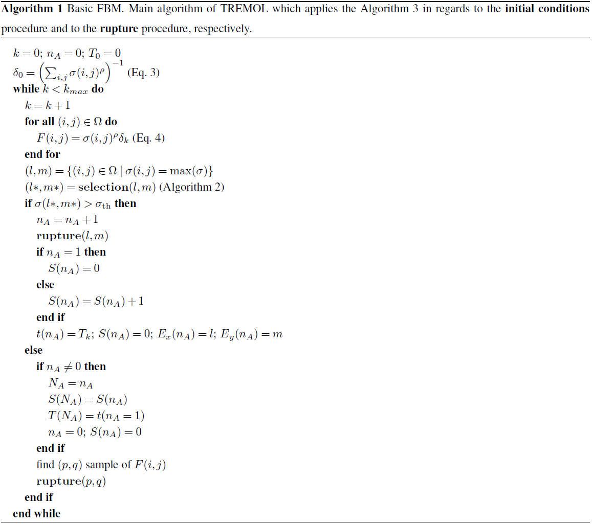
TREMOL is based on the probabilistic formulation of the FBM, with the failure rate of a set of fibers given by Eq. (1): (Gómez et al., 1998; Moral et al., 2001).
where U(t) is the number of fibers that remain unbroken at time t. The hazard rate K(σ(t)) is a function of the fiber stress σ(t). Experimental results show that the hazard rate of materials under constant load can be well-described by the Weibull probability distribution function. This behavior can be summarized in Eq. (2) (Coleman, 1958; Phoenix, 1978; Phoenix and Tierney, 1983; Vázquez-Prada et al., 1999; Moreno et al., 2001; Biswas et al., 2015):
where ν0 is the reference hazard rate, and σ0 the reference stress. The Weibull exponent, ρ, quantifies the nonlinearity (Yewande et al., 2003). If , the expression in Eq. (2) can be simplified to K(σ(t))=σ(t)ρ. From the probabilistic formulation, two equations arise (Eqs. 3 and 4), which are applied in our algorithm to define the system dynamics. The details of these two equations are described below.
- a)
Gómez et al. (1998) and Moral et al. (2001) developed a relation to compute the expected rupture time (dimensionless) of the fibers following Eqs. (1) and (2). This expected rupture time interval is defined as δk (Eq. 3) and can be applied to any load-transfer rule:
where N is the total number of cells, and σi is the load in the ith cell. The dimensionless cumulative time, T, is the sum of δk.
- b)
The failure probability, Fi, which is a function of the load σi in each cell, is (Moreno et al., 2001)
The dynamic values δk and Fi are updated with each time step due to rupture processes and the resulting load transfer.
A suitable FBM algorithm to simulate earthquakes should consider a complex stress field, physical properties of materials, stress transfer between faults (at short and long distances), and dissipative effects. Using the FBM we assume that earthquakes can be considered analogous to characteristic brittle rupture of a heterogeneous material (Kun et al., 2006a, b).
The previous basic concepts about the FBM were considered for the development of the TREMOL code, with the purpose of modeling the behavior of seismic asperities. In the next section, we describe the details of this code.
Since the main objective of TREMOL is to simulate the rupture process of seismic asperities based on the principles of the FBM, we model two materials with different mechanical properties interacting with each other.
In order to introduce the features of TREMOL we describe three main stages during the application of TREMOL.
- 1.
Preprocessing
In this stage we have to assign the following input data:- -
the size of the fault plane,
- -
the size of the maximum asperity within the fault plane, and
- -
other parameters (load-transfer value π, strength value γ, initial load values σ, and load threshold σth).
- -
- 2.
Processing
TREMOL uses the data from the preprocessing stage to carry out the FBM algorithm, and by applying Eqs. (3) and (4) the rupture process is computed in the fault plane studied. The asperity size of each earthquake is used by TREMOL to also compute the magnitude of each synthetic earthquake. - 3.
Post-processing
In this stage, TREMOL summarizes the results that are computed in the processing stage and computes the equivalent rupture area (km2). In general, TREMOL output generates a synthetic catalog of earthquakes, which consists of the following:- -
total number of earthquakes that can occur in the fault plane studied,
- -
size of the asperity of each earthquake, and
- -
magnitude of each earthquake.
- -
In the next sections we describe with more detail each one of the three main stages during the application of TREMOL. An overview of the entire simulation process is shown in Fig. 1.
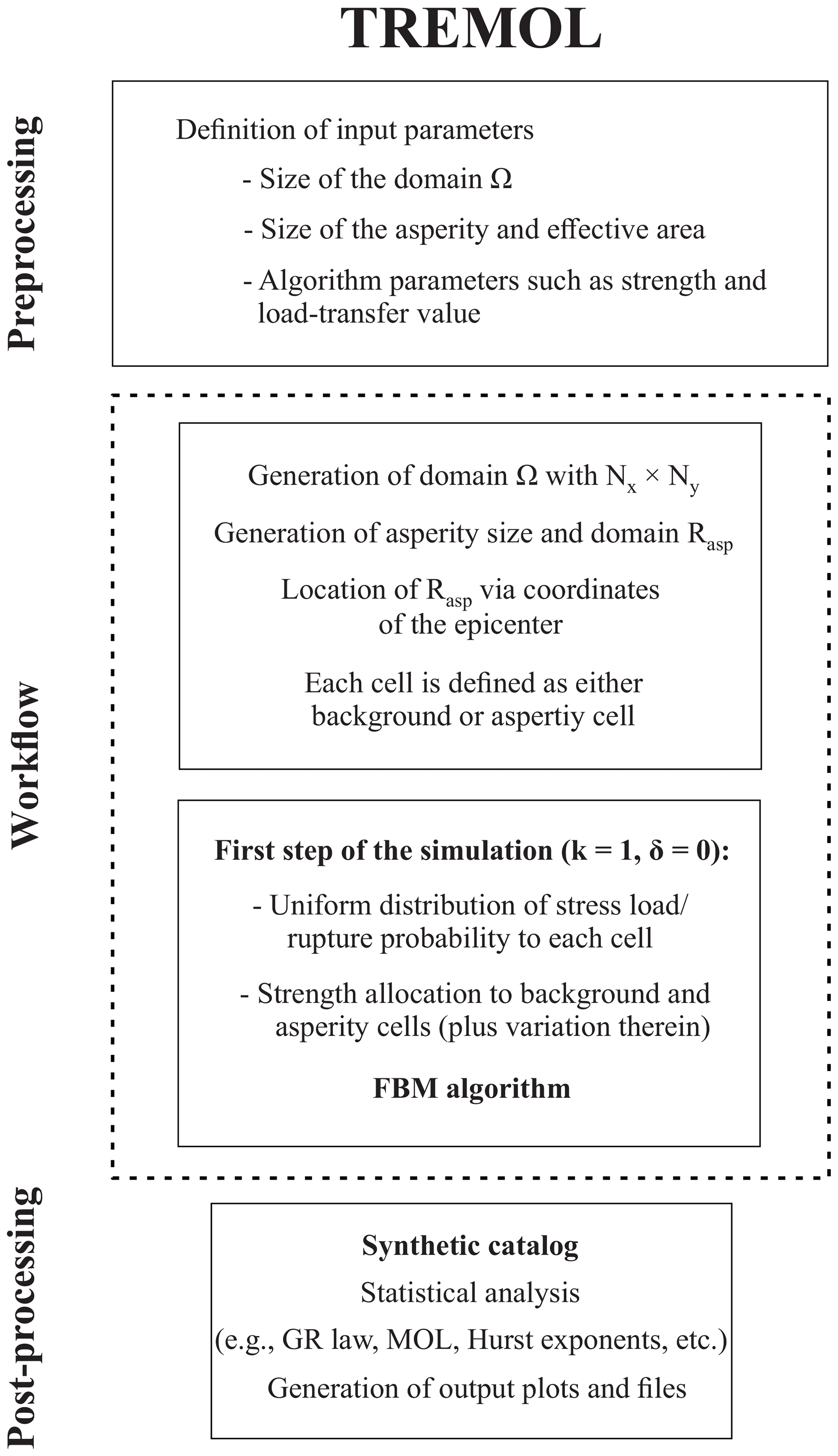
Figure 1TREMOL flowchart. At the beginning (preprocess) the algorithm initiates a domain Ω with Nx×Ny cells in which every cell is either part of an asperity or of the background or fault plane. Afterwards (first time step, k=1) a uniform distribution allocates a random stress load and rupture probability to all cells. In addition, asperity cells obtain a random strength value from a uniform distribution. Next (time step k≥2) the failure process starts following the FBM algorithm. After every failure the stress of the broken cell is redistributed via the LLS rule and the number of time steps (k) increases by 1 until the target number of time steps is reached. If the final number of time steps has been reached the simulation stops. At the end, all information about the entire failure process is saved in a database or a synthetic catalog that can be used for statistical analysis. Further details about the algorithm are given in Sect. 3.
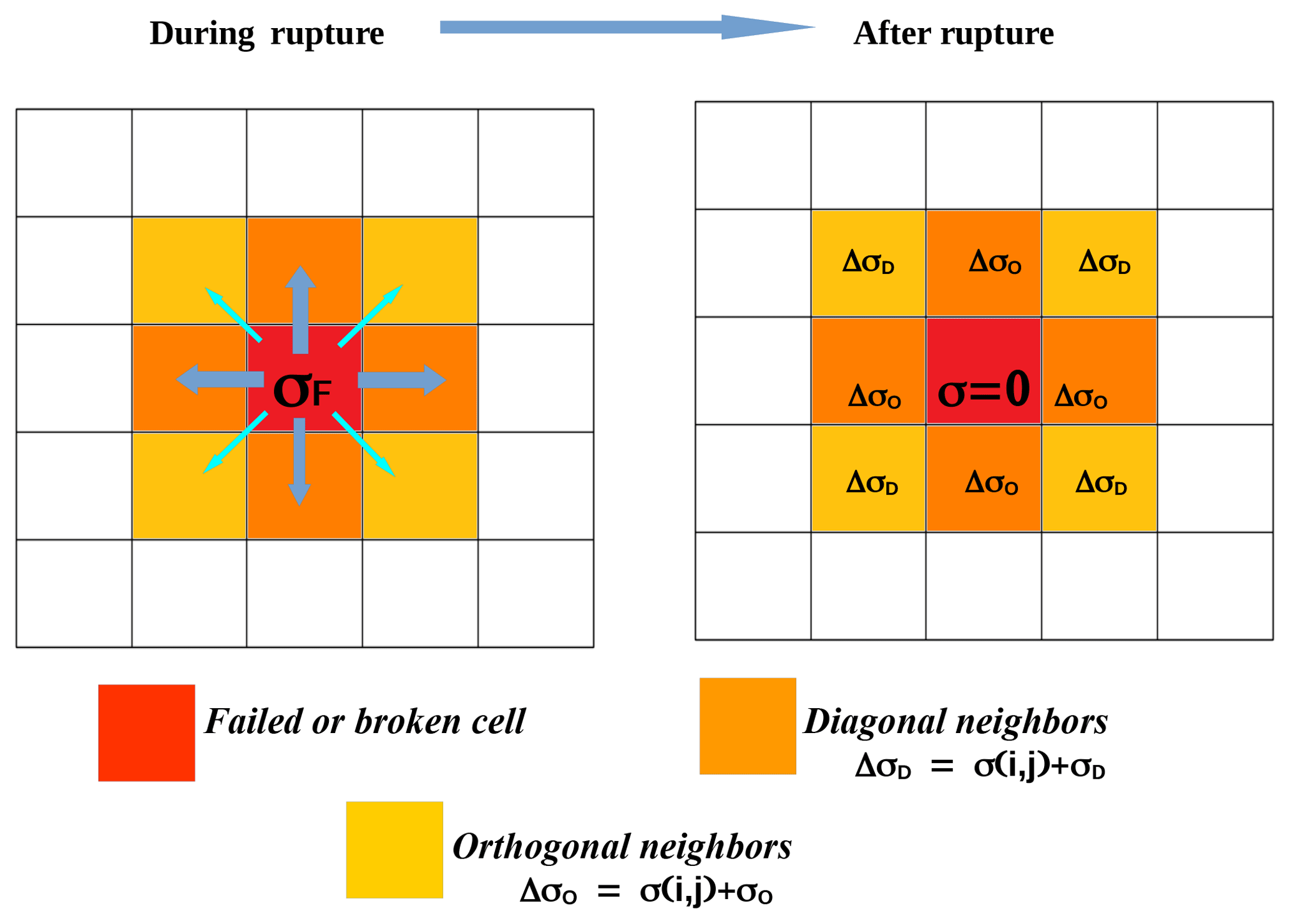
Figure 2Schematic representation of the considered local load rule. The broken cell with load, σF, distributes the largest load fraction, σO (Eq. 5), to its four orthogonal neighbor cells. The remaining load, σD (Eq. 6), is transferred to its four diagonal neighbor cells. Afterwards, the load of the broken cell drops to zero, σ=0. Asperity cells cannot receive any new load.
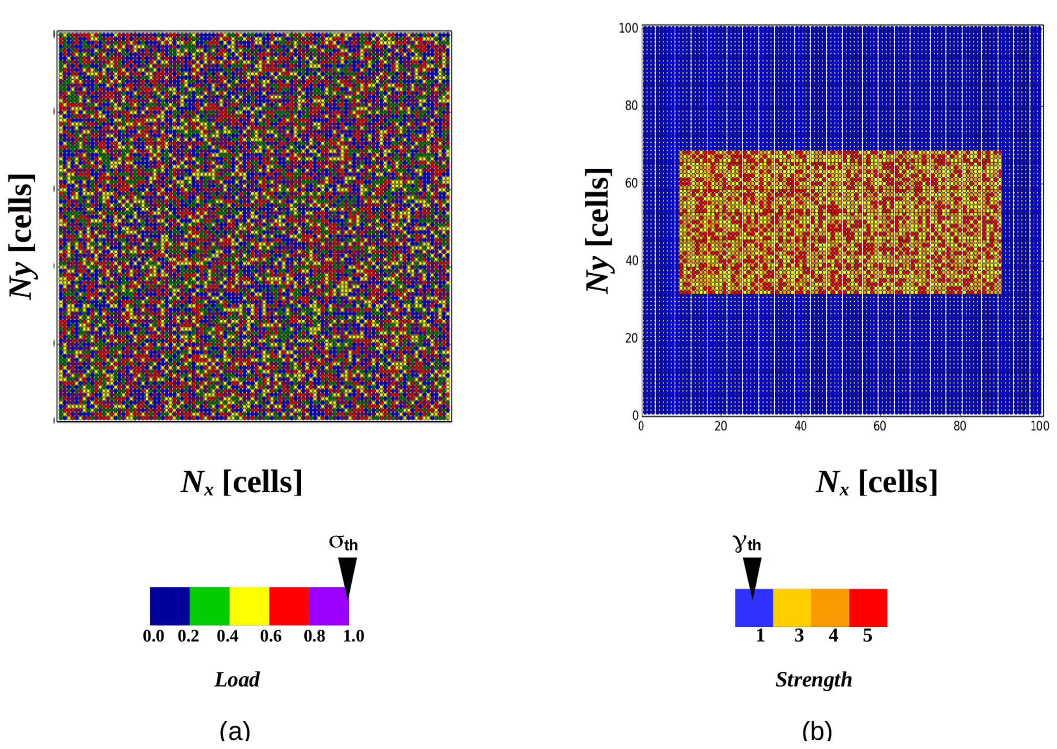
Figure 3(a) Spatial distribution of the random initial loads σ(i,j). RAsp represents a rectangular fault plane of cells. The color bar indicates the load and the threshold load of σth=1. (b) Spatial distribution of the strength γ(i,j). Two main regions can be distinguished in this figure: (1) the asperity region defined as the inner rectangle and (2) a background area or fault plane. While the asperity contains strength values in the range of 3 to 5, the rest of the fault plane has a strength value of 1.
3.1 Preprocessing: input data and initial conditions
In TREMOL, a fault plane is modeled as a rectangle (Ω), which is divided into Nx×Ny cells. Each cell is defined by its position (i, j), where and . In the fault plane Ω earthquakes can occur with different magnitudes. Additionally, it is possible to assign to each fault plane an asperity region (RAsp).
To define each fault plane (Ω) and its respective asperity region (RAsp) it is necessary to assign specific properties to their cells. Particularly, it is necessary to define three properties (or values) for each cell of Ω and RAsp: a load σ(i,j), a strength value γ(i,j), and a load-transfer value π(i,j).
-
The load σ(i,j). At the beginning of each realization, TREMOL randomly assigns a value of the load σ(i,j) to each cell of Ω using a uniform distribution function (). This assumption simulates a heterogeneous stress field. Moreover, a load threshold σth=1 is necessary to create a limit at which a cell must fail (Moreno et al., 2001). At the end of this step any cell within Ω must have a load value between 0 and 1.
-
The strength value γ(i,j). This parameter represents an analogy to the concept of hardness or strength. In our model, the algorithm will find it difficult to break a cell if this cell has a value γ>1 since the strength threshold before failure is set as γth=1 (see a detailed explanation in Sect. 3.2). As a result, a strength γ>1 may simulate a hard material that needs to be weakened before it can fail. This process can be regarded as similar to material fatigue or creep failure. The strength value for all cells in RAsp, namely γAsp, is chosen in a discrete interval of , where 𝒰D is an integer uniformly distributed and γRef is an assigned reference value.
-
The load-transfer value π(i,j). This parameter represents the percentage of load that can be distributed from a ruptured cell to its neighbors. In this study, the load in the ruptured cell is called σF(i,j). TREMOL uses a local load sharing (LLS) rule considering the eight nearest neighbors. According to previous studies, such as Monterrubio-Velasco et al. (2017), TREMOL redistributes the majority of the load to the four orthogonal neighbors. The load that is transferred to these orthogonal neighbors is called σO, and it is defined according to Eq. (5):
where πF is the load-transfer value of the failed cell. Additionally, a small proportion of the load is transferred to the four diagonal neighbors. The value of this load is called σD(i,j), and it is defined according to Eq. (6):
The assumption of Eqs. (5) and (6) is in agreement with what is expected for the maximum shear stress directions with respect to the main stress orientation that gives rise to both synthetic and antithetic faulting (e.g., Stein and Wysession, 2008). Figure 2 is a schematic representation of the load distribution process from the failed cell, σF(i,j) (in red), to its nearest neighbors.
In order to differentiate the parameters of the asperity from the rest of the fault plane Ω, we define πAsp(i,j) and γAsp(i,j) that refer only to the cells within RAsp. For the rest of the fault plane Ω, we are using the same parameters defined previously: π(i,j) and γ(i,j). Figure 3a shows an example of the randomly distributed initial load throughout the fault plane. Figure 3b displays an example of differences between the strength of the asperity and the rest of the fault plane.
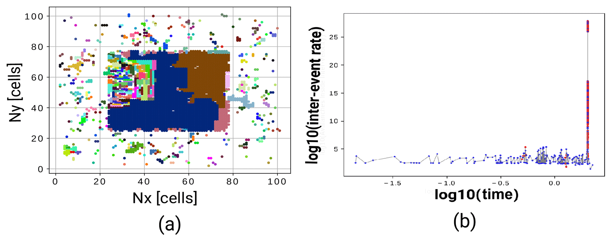
Figure 4Results of one realization by TREMOL. (a) The spatial distribution of avalanches. Patches of the same color indicate one temporal-consecutive Avalanche cluster (synthetic earthquake). (b) Logarithmic representation of the inter-event rate with time. The red dots represent the inter-event rate when the asperity rupture occurs. The blue dots indicate foreshocks.
3.2 Main computational processes
Once the initial information for the entire domain Ω is defined, the core algorithm of TREMOL will realize a transfer, accumulation, and rupture process. While the cells interact with each other, there are two basic failure processes depending on the load of the cell in comparison with the threshold load (Moreno et al., 2001).
-
Normal event. If all cells within the system have a load , a normal event is generated, and the cell that will fail is randomly chosen considering the individual failure probability of each cell, F(i,j) (Eq. 4).
-
Avalanche event. If one or more cells have a load value , an avalanche event is generated, and the cell that fails is the one with the greatest σ(i,j) value.
Due to the integrated strength property some extra rules for rupture are necessary. The requirement for failure is . On the other hand, if a cell with is chosen, its strength is reduced by one unit. This strength condition enables us to simulate a material weakening process during the load-transfer process. Additionally, this condition offers the possibility to produce large load accumulations locally, which are more likely to generate larger ruptures.
When a cell within RAsp breaks it becomes inactive until the end of the simulation, which means it cannot receive any further load. The large load concentration within the asperity usually produces a very short time interval (Eq. 3), with the result that there is physically not enough time available to reload the stress on an asperity right after its rupture. On the contrary, a cell outside of the asperity region remains active after its failure but its load drops to zero. The simulation ends when all the cells within the asperity have become inactive.
3.3 Output data and post-processing
After every execution TREMOL outputs a catalog detailing where the position (x,y) of the failed cell, the rupture time (Eq. 12), the avalanche event or normal event identification, the mean load, and many other values are saved for each time step. We cluster avalanche events considering the time and space criterion. We assume and are two consecutive avalanche events generated in chronological order. If their Euclidean distance is Δri≤rth (where ), then ai and ai−1 will belong to the same cluster. This clustering algorithm is applied to all generated avalanche events. Lastly, we extract a new catalog that shows the size of each cluster, the position of the first element of each cluster related to the nucleation point, and the time when it was initiated. This database is our simulated seismic catalog. Note that the cluster size is given in nondimensional units. However, we use an equivalence between Ω and an effective area Aeff in order to obtain a physical rupture area. Finally, each cell can represent an area in square kilometers. This step is necessary in order to compute an equivalent magnitude, which is comparable with real earthquake magnitudes. For this purpose, we use three magnitude–area relations. In particular, we use Eqs. (7), (8), and (9) obtained by Rodríguez-Pérez and Ottemöller (2013) for Mexican subduction earthquakes:
where Aa is the asperity area (km2). Equation (7) was obtained from asperities defined by the average displacement criterion (Somerville et al., 1999). Equations (8) and (9) were computed from asperities defined by the maximum displacement criterion for a large asperity and a very large asperity, respectively (Mai et al., 2005).
Furthermore, we define the inter-event rate Δνk as analogous to the rupture velocity:
where Δrk is the inter-event Euclidean distance between the k event located at (xk,yk) and k−1 event in .
The inter-event time Δδk is computed following
where δk is given by Eq. (3). Figure 4a shows an example of the final spatial distribution of rupture clusters for a particular example. Each cluster is indicated by the same color and represents a simulated earthquake. Figure 4b shows the related inter-event rate. The inter-event rate largely increases when the asperity rupture occurs.
In the post-processing step we additionally computed the rupture duration of the largest simulated earthquake, DAval, using the rupture velocity and the effective fault dimensions obtained from finite-fault models (Table 5).
We used Eq. (13) (Geller, 1976) to compute DAval:
where
Using these considerations, we can assign a physical unit of time (s) to the largest simulated earthquake, .
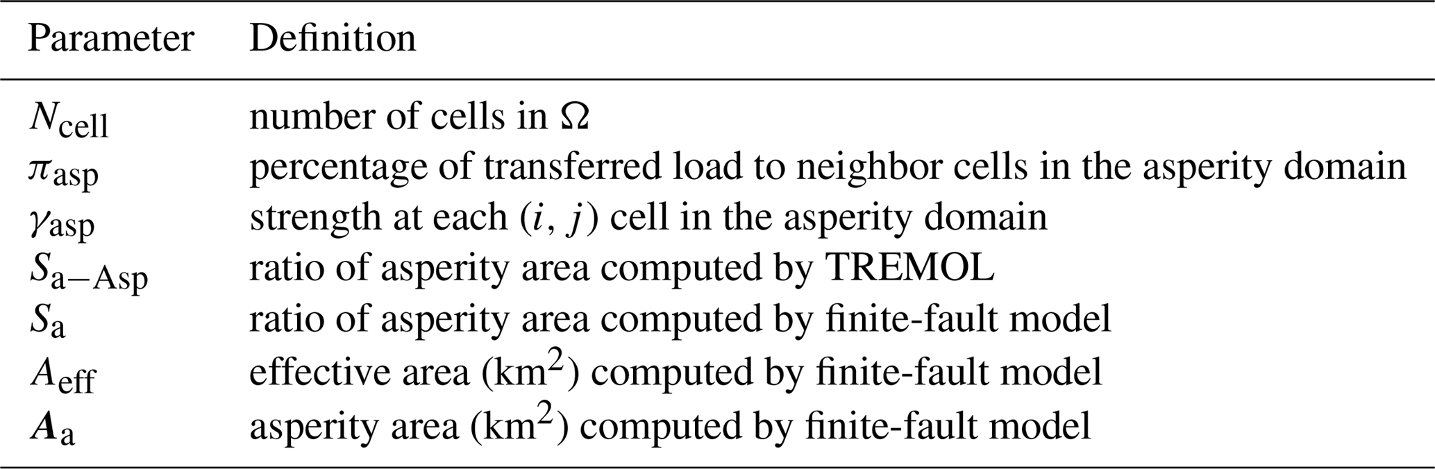
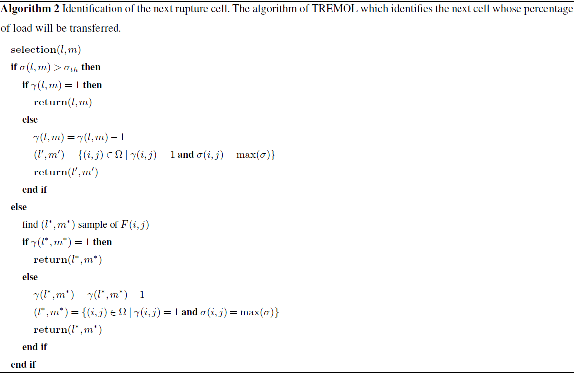
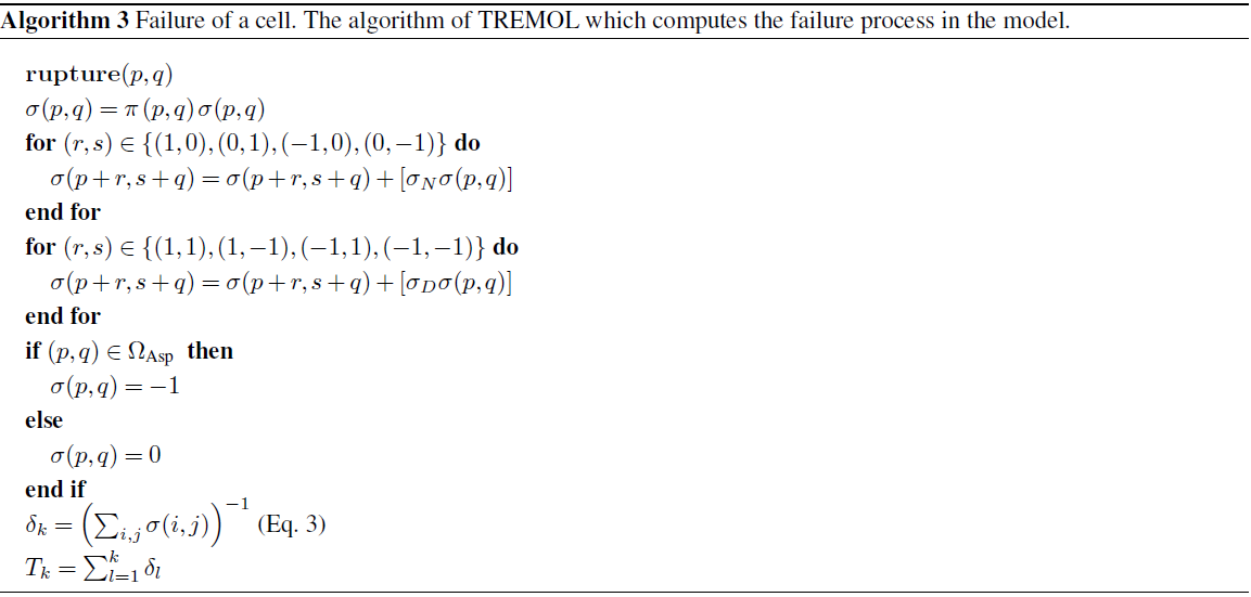
The flowchart in Fig. 1 and the pseudo-codes 1, 2, and 3 summarize the algorithm of TREMOL. A summary of all required parameters to execute the TREMOL code are shown in Table 1.
Table 1TREMOL preprocessing: input parameters and their definition.
4.1 Methods: parametric study
We performed a sensitivity analysis of the three asperity parameters (γasp, Sa−Asp, and πasp) in order to identify the best combination that produces the best approximation to real data, such as the maximum rupture area, Asyn, and its related magnitude Msyn. In order to investigate the influence of every single parameter, we statistically determined how the results vary with different parameter configurations.
4.1.1 Percentage of transferred load, πasp – methods
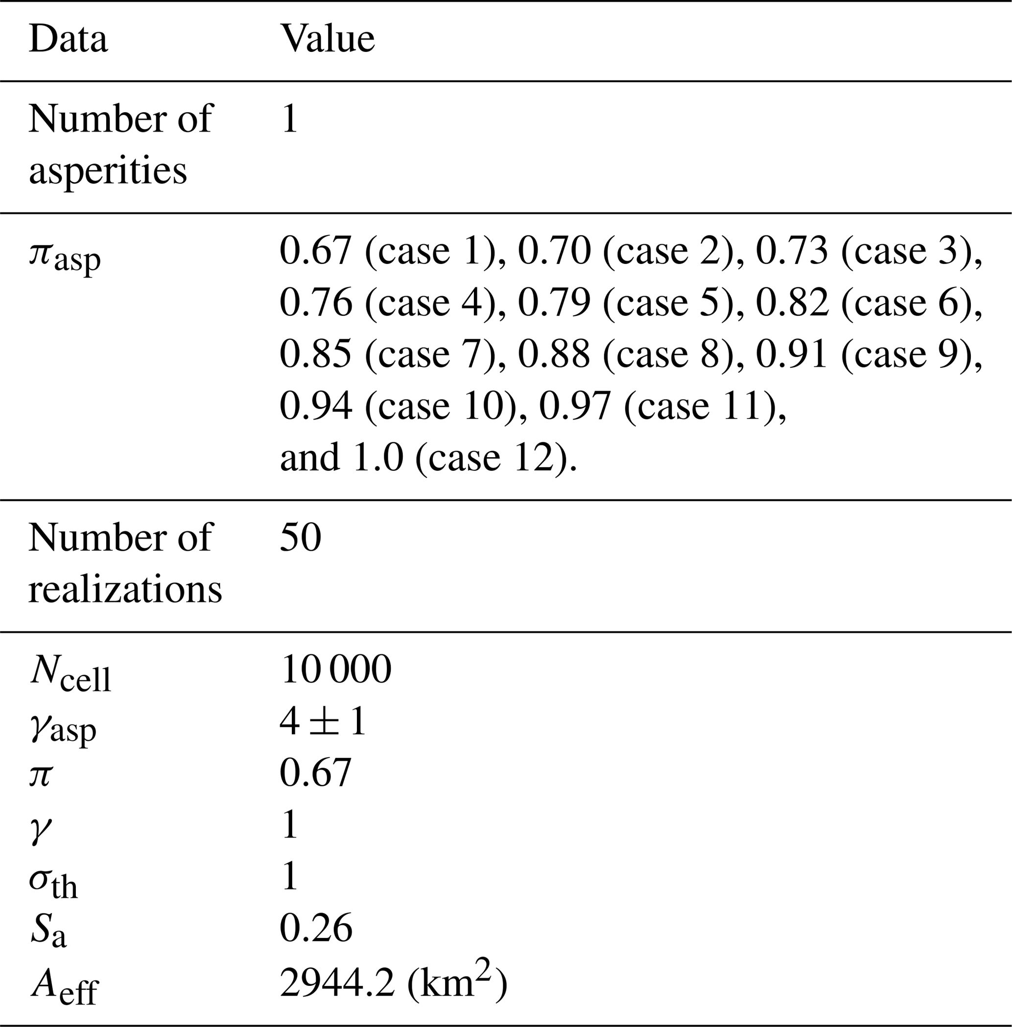
To explore the influence of πasp, we analyzed 12 values (, with increments of 0.3). The minimum πasp=0.67 assigns the same value to an asperity cell and to a background cell. On the other hand, πasp=1.0 means that the load in a failed asperity cell is fully transmitted to the neighbors (ideal case with no dissipative effects). Note that πasp=1 does not represent real physical conditions since dissipative effects are ignored completely. On the other hand, if πasp=0.67 (case 1) the asperity cells would transfer as much load as the cells in the background. The objective is to generate a load concentration within the asperity that corresponds to the largest magnitude. If the asperity cells transfer as much load as the background cells, no such load concentration can be obtained. As a result, we can expect that the mean Asyn for πasp=0.67 (case 1) is the lowest value in comparison to all other cases.
The input data of this experiment are summarized in Table 2. We assigned a strength to the asperity (RAsp) and a value of γBkg=1 to the rest of the fault plane. These values are chosen after experimental trials, which have shown that the difference is large enough to simulate a significant strength difference with low computational effort. To define the effective area and the asperity size, we chose the values computed for the earthquake of 20 March 2012, Mw=7.4, in Rodríguez-Pérez and Ottemöller (2013): Aeff=2944.2 km2 and Sa=0.26. We defined the size of Ω consisting of Ncell=10 000 cells in total. We carried out 50 simulations per πasp configuration. In addition, we modified the random seed to have different initial load configurations, σ(i,j), to ensure that the results over πasp are independent of the initial load conditions σ(i,j).
4.1.2 Strength parameter, γasp – methods
To perform the parametric study of γasp, we configured two asperities embedded in Ω. In this experiment, the total size is cells. Afterwards, we located each asperity in the center of the two sub-domains Ω′ of 100×100 cells. Figure 5 shows a schematic representation of the domains Ω and Ω′ used in this experiment.
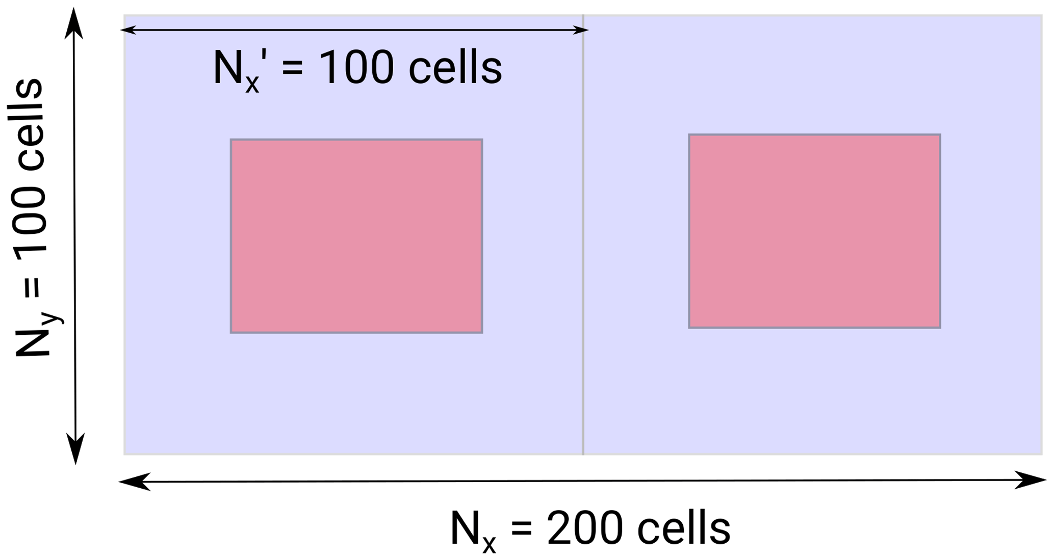
Figure 5Schematic configuration for the parametric study of γasp and Sa−Asp. The size of the domain Ω is cells. Each asperity is located within the center of the two sub-domains Ω′ of 100×100 cells. The strength parameter γasp and degree of heterogeneity for each asperity can be varied according to the material properties.
The separation between the two asperities remains constant. We chose a value of πasp=0.90 to produce a large contrast between the asperity and the rest of the fault plane (π=0.67) (Monterrubio-Velasco et al., 2017). In order to analyze the influence of γasp (and Sa−Asp), the asperity on the right-hand side (Asp. 2) has varying strength values, while the strength of the left asperity (Asp. 1) remains constant. Finally, the maximum ruptured area and magnitude generated in each Ω′ are computed.
In order to explore how the system behaves when γasp changes, we analyzed six different values of (cases 13 to 18). The input data used in this test are summarized in Table 3. We defined the same asperity size for both: . In Fig. 6, we show an example of the spatial configuration of this analysis. The background strength is considered to be constant, and the color bar indicates the γ(i,j) values.
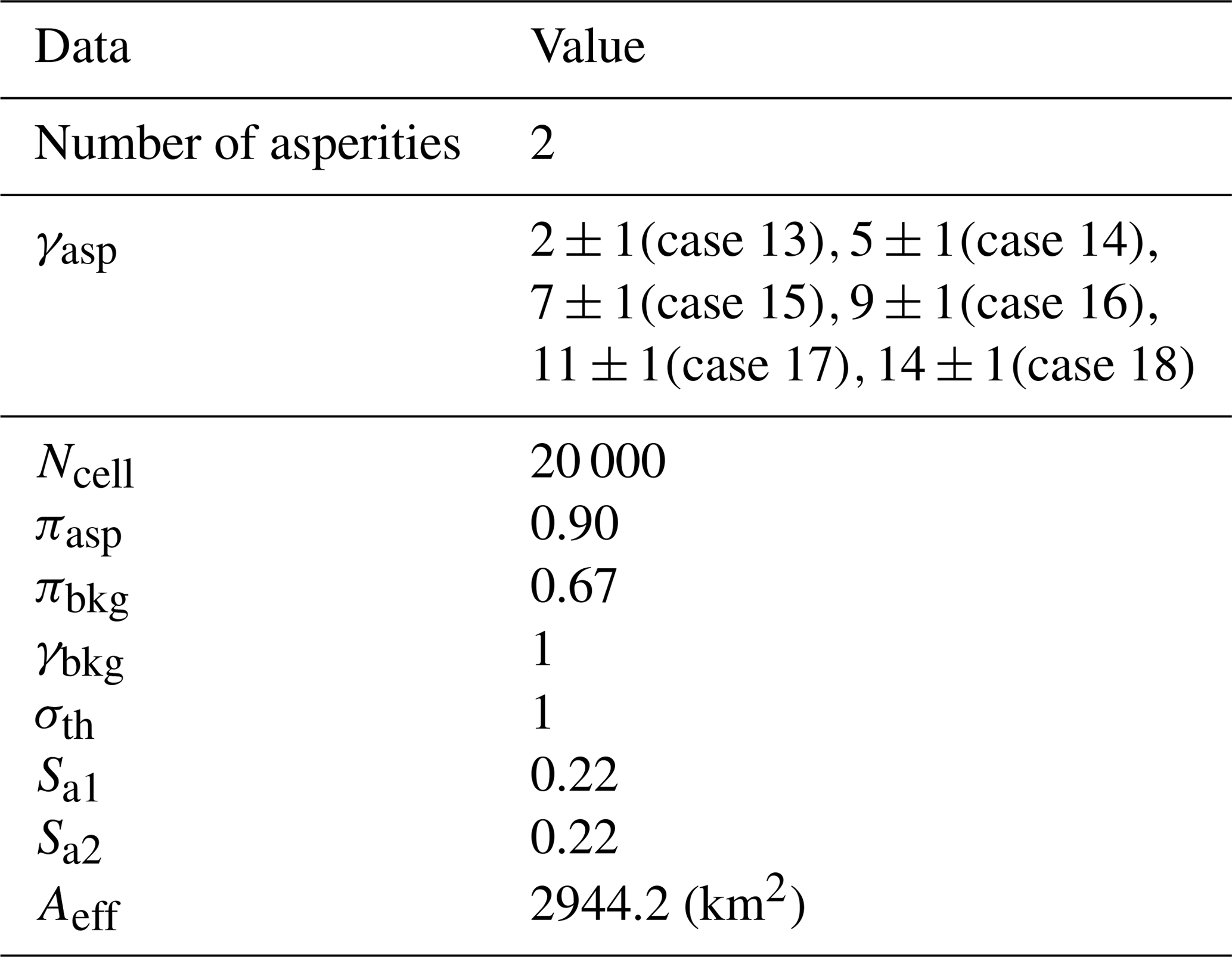

Figure 6Example of the strength configuration γ(i,j) for the sensitivity analysis of γasp. Two asperities with the same size are defined and embedded in Ω following the schema in Fig. 5. The conservation parameters are πasp=0.90 and πasp=0.67. The color bar indicates different γ(i,j) values. The left asperity (Asp. 1) contains constant properties, while the right asperity (Asp. 2) has variable strength values.
4.1.3 Asperity size, Sa−Asp – methods
The modification of the Sa−Asp parameter was based on the same configuration as described in the previous section. We analyzed six different values of the asperity size Sa (cases 19 to 24). In Fig. 7 we show an example of the asperity configuration in which the left asperity (Asp. 1) has a constant size Sa2, while the size of the right one (Asp. 2) increases. In this experiment, we considered and πasp=0.90. The main data related to these six cases are summarized in Table 4.
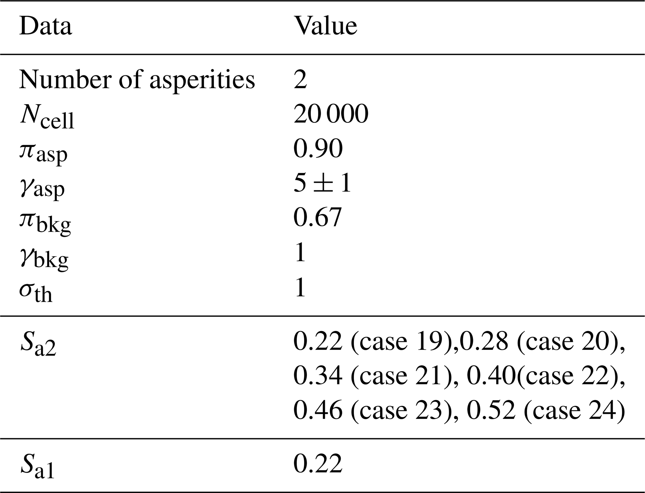
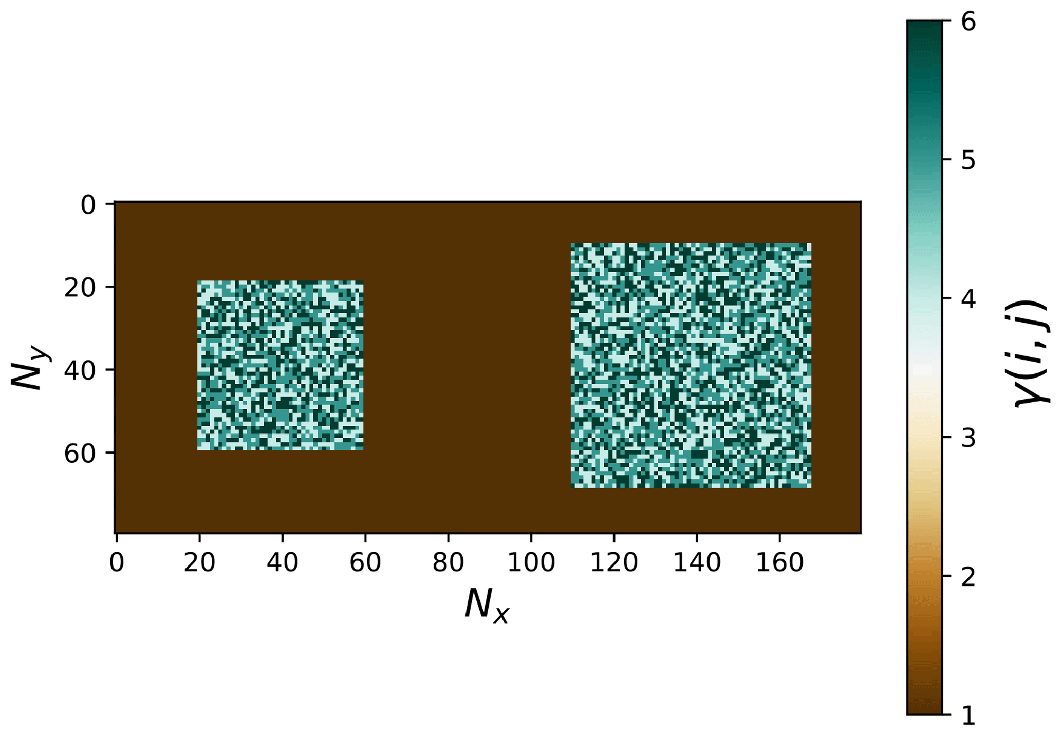
Figure 7An example configuration of different asperity sizes, Sa−Asp. The color bar indicates the strength γ(i,j) values used during the test.
4.2 Model validation – methods
We evaluated the capability of the model to reproduce the characteristics of 10 Mexican subduction earthquakes (eight shallow thrust subduction events, ST, and two intra-slab subduction events, IN). The input data of the effective area, Aeff, and the asperity ratio size, Sa, are given from waveform slip inversions and seismic source studies ( and ) shown in the database of Mexican earthquake source parameters by Rodríguez-Pérez et al. (2018). This database includes results from two different methodologies: spectral analysis and finite-fault models. From the latter, the database provides estimations of effective fault dimensions, rupture velocity, source duration, number of asperities, stress, and radiated seismic energy on the asperities and background areas. Slip solutions were obtained with teleseismic data for events with .
The number of cells was Ncell=10 000 for a domain Ω of 100×100 cells. We modeled the size of Ω proportionally to the size of Leff and Weff for each scenario according to the following equations, Eqs. (15) and (16):
where Nx and Ny are the number of cells in the x axis and y axis, respectively. As an example, Fig. 8 presents the size and aspect ratio of Ev. 3 and Ev. 5 (Table 5).
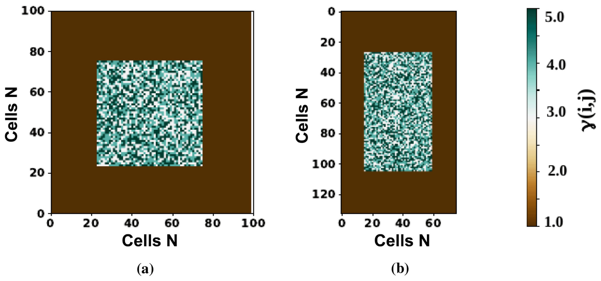
Figure 8Example of the domain configuration Ω, considering Leff and Weff. (a) Example configuration of event 3 and (b) example configuration of event 5. The required data can be found in Table 5.
In some cases, the number of asperities computed in Rodríguez-Pérez et al. (2018) is greater than 1. However, as a first approximation we simplified the problem by modeling only one asperity per earthquake.
In order to study how the asperity size Sa affects the maximum ruptured area, we randomly modified the size as
where is a random value. We introduce this assumption because we want to avoid a preconceived final size. In future trials it may be useful to consider the inner uncertainties of finite-fault models. The asperity aspect ratio follows the same proportion as the effective area, (Fig. 8).
We carried out 50 realizations per event (Table 5), changing the size Sa−Asp in each one (Eq. 17).
Rodríguez-Pérez and Zúñiga (2016)Mendoza (1989)Rodríguez-Pérez and Ottemöller (2013)Rodríguez-Pérez and Ottemöller (2013)Rodríguez-Pérez and Ottemöller (2013)Rodríguez-Pérez and Ottemöller (2013)Rodríguez-Pérez and Ottemöller (2013)Rodríguez-Pérez and Ottemöller (2013)Table 5The finite-fault source parameters used in this work. Weff and Leff are the effective fault dimensions (width and length, respectively, according to Mai and Beroza, 2000). Areal is the asperity area, Aeff is the effective rupture area (Weff×Leff). Duration is the rupture duration computed from the slip inversion, Na is the number of asperities, and Vr is the rupture velocity. Ratio is the aspect ratio of the fault area. The type of the event is labeled ST for shallow thrust and IN for intra-slab events.

4.2.1 Modeling the rupture area and magnitude of 10 subduction earthquakes – methods
In this case the number of cells is Ncell=10 000 (100×100). We carried out 50 executions per event and in each execution we randomly changed the size Sa−Asp following Eqs. (15), (16), and (17). The input data of the 10 modeled earthquakes in Table 5 are summarized in Table 6.

4.2.2 Case study (Oaxaca, Mw=7.4, 20/03/2012): using different effective areas Aeff for the same event – methods
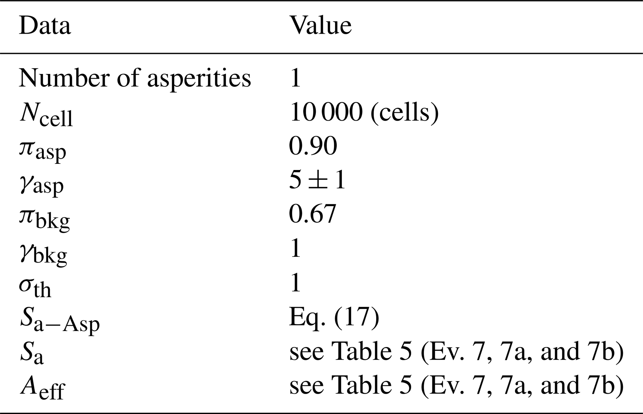
As reported in Rodríguez-Pérez et al. (2018) for some events, there are several solutions that allow us to analyze the variability in the estimated source parameters (see parameters of events 7, 7a, and 7b in Table 5). In this study, we applied TREMOL to study how the ruptured area and the assessed magnitude change when we use different input data to model the same earthquake. The data related to these three events are summarized in Table 7.
Table 7Main data for the case study Ev. 7 test, Ev. 7a test, and Ev. 7b test.
4.2.3 Assessing a future earthquake in the Guerrero seismic gap: rupture area and magnitude – methods
We apply our method for the estimation of possible future earthquakes, in particular to compute the expected magnitude, since TREMOL may offer new insights for future hazard assessments. We carried out a statistical test to assess the size of an earthquake that may occur in the Guerrero seismic gap (GG) region.
As input parameters, we used the area found by Singh and Mortera (1991): km. We defined the asperity size ratio Sa as proposed by Somerville et al. (2002) for regular subduction zone events (SB) based on average slip, Sa=0.25. Singh and Mortera (1991), Astiz et al. (1987), and Astiz and Kanamori (1984) proposed a probable maximum magnitude for this region of . Therefore, using the effective rupture area (Leff, Weff, and Sa), we executed the algorithm as in previous sections. The input data related to this analysis are summarized in Table 8. Likewise, we want to estimated the duration Daval of the event. To compute this value, we used a mean of the Vr from Table 5.
Table 8Main data for assessing a future earthquake in the Guerrero seismic gap (GG event).

5.1 Results: parametric study
5.1.1 Percentage of transferred load, πasp
Figure 9 shows the mean (black dots) of the maximum ruptured area Asyn, including the upper and lower limits of the standard deviations (blue squares), after the execution of all 12 cases (Table 2) with 50 realizations. The value of Asyn is related to the largest produced cluster in Ω. There are two dominant tendencies identifiable.
-
If πasp<0.76, the mean of the maximum ruptured area increases continuously more than 1 order of magnitude from 15 to ≈500 km2, i.e., an increase of 3333 %. The standard deviation of Asyn for πasp=0.7 is ≈35 km2 (100 % error).
-
If πasp≥0.76 (cases 4 to 12), the Asyn values remain essentially constant (≈500 km2). Likewise, the upper and lower limit vary around the same order. The standard deviation for this interval is ≈100 km2 (20 % error).
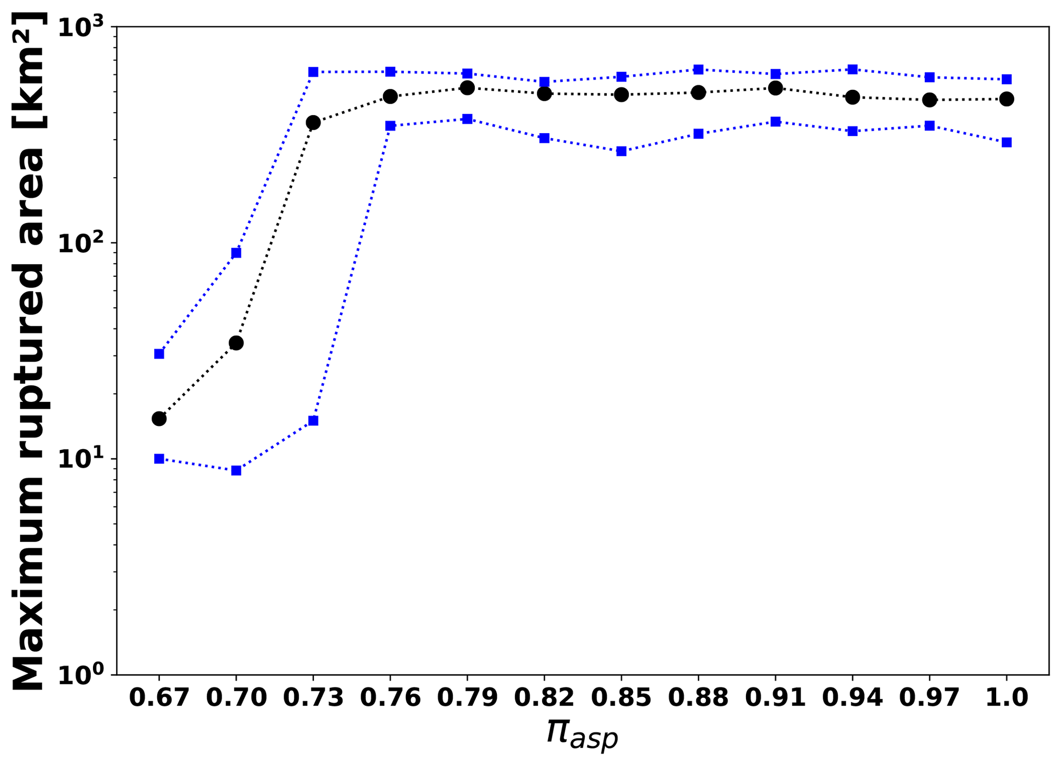
Figure 9Mean of the maximum rupture area (km2), Asyn, for different values of πasp depicted as black circles. The minimum and maximum limits of the rupture area are represented by blue squares.
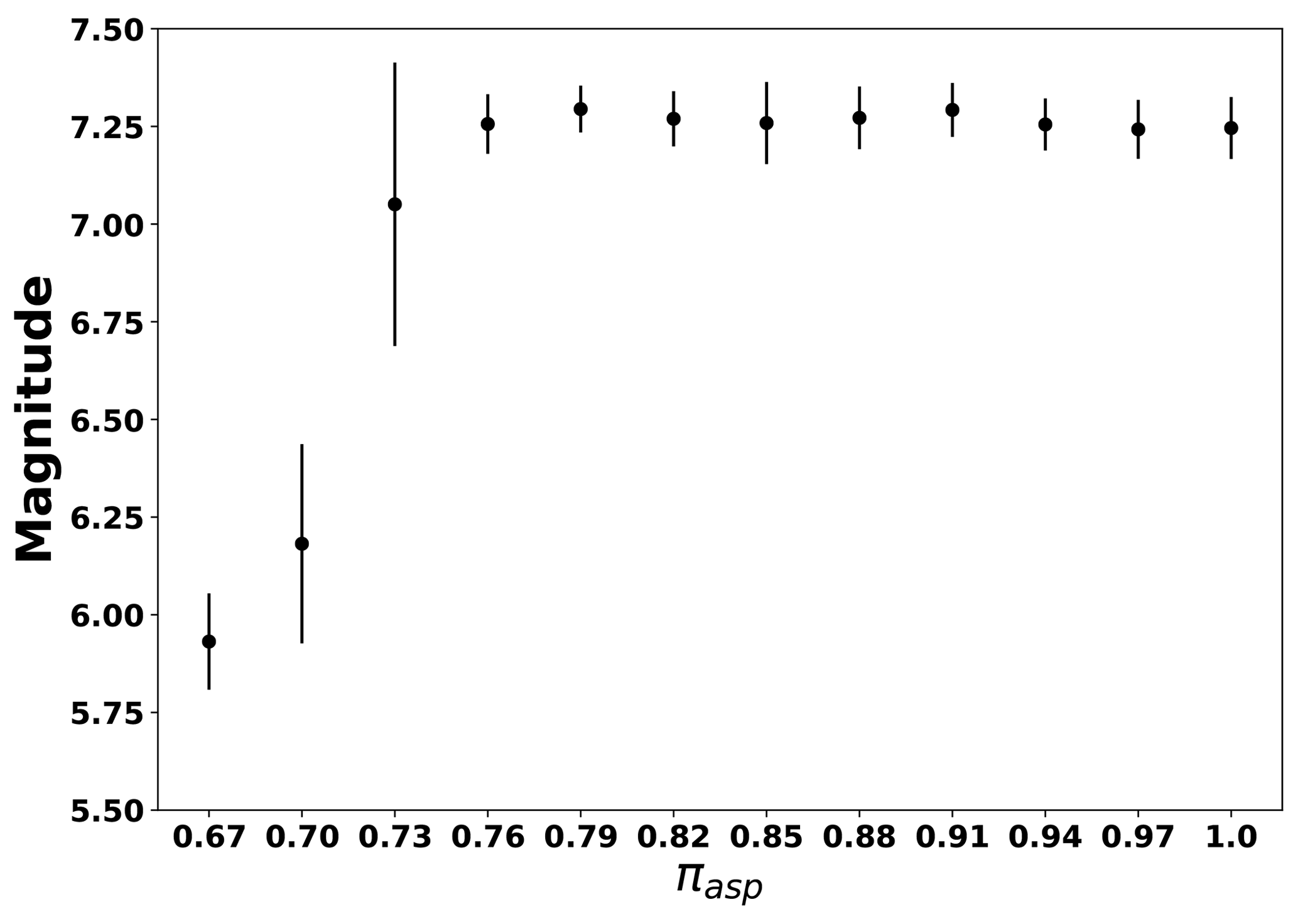
Figure 10Mean and standard deviation of the maximum magnitude over 50 realizations depending on πasp.
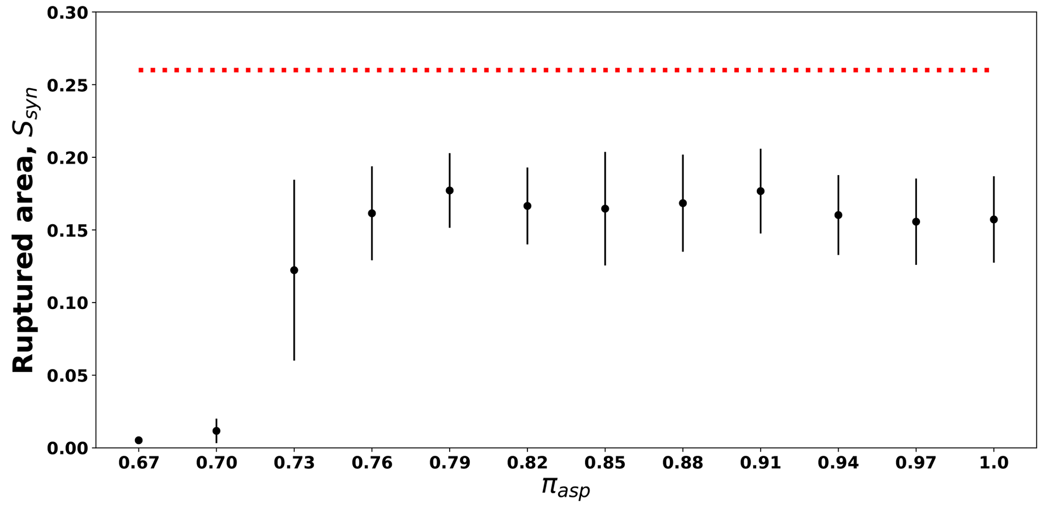
Figure 11Mean and standard deviation of the ratio over 50 realizations for different values of πasp. The red line indicates the asperity ratio Sa computed for event 7 (Table 5).
Using the mean of Asyn obtained in each case, we computed the corresponding magnitude. The results are given as the mean and standard deviation of the maximum magnitude in Fig. 10 for all 12 cases (see Table 2). Due to the fact that ruptured area and magnitude are correlated (see Eqs. 7, 8, and 9), the pattern in Fig. 10 is very similar to the one in Fig. 9.
Overall, there are three aspects observable.
-
If πasp≥0.76 (cases 4 to 12), the mean magnitudes show a steady value (≈7.2).
-
If , a transition with an increasing trend with the largest standard deviation is visible.
-
If πasp=0.67 (case 1), the mean of the maximum magnitude is the lowest.
In this experiment, the initial value of Sa=0.26 remains constant; i.e., the asperity size does not increase randomly (red line in Fig. 11). After executing all configurations, we computed the ratio of , relating to the largest ruptured area. We show the mean and standard deviation of this ratio Sa−Asp in Fig. 11. We observed that the ratio of Sa−Asp is always ≈0.10 lower than Sa.
5.1.2 Strength parameter, γasp
For each value of γasp (Table 3), we performed 50 executions while changing the initial strength parameter of the asperity γasp (Fig. 3b). Likewise, we computed the maximum magnitude obtained for each Ω′. Figure 12 indicates the mean and standard deviation of the computed maximum magnitude with a dependence on γasp. The upper subplot (blue markers) shows the results for the left (constant) asperity (Asp. 1). The lower subplot (red markers) shows the results for the right (variable) asperity (Asp. 2).
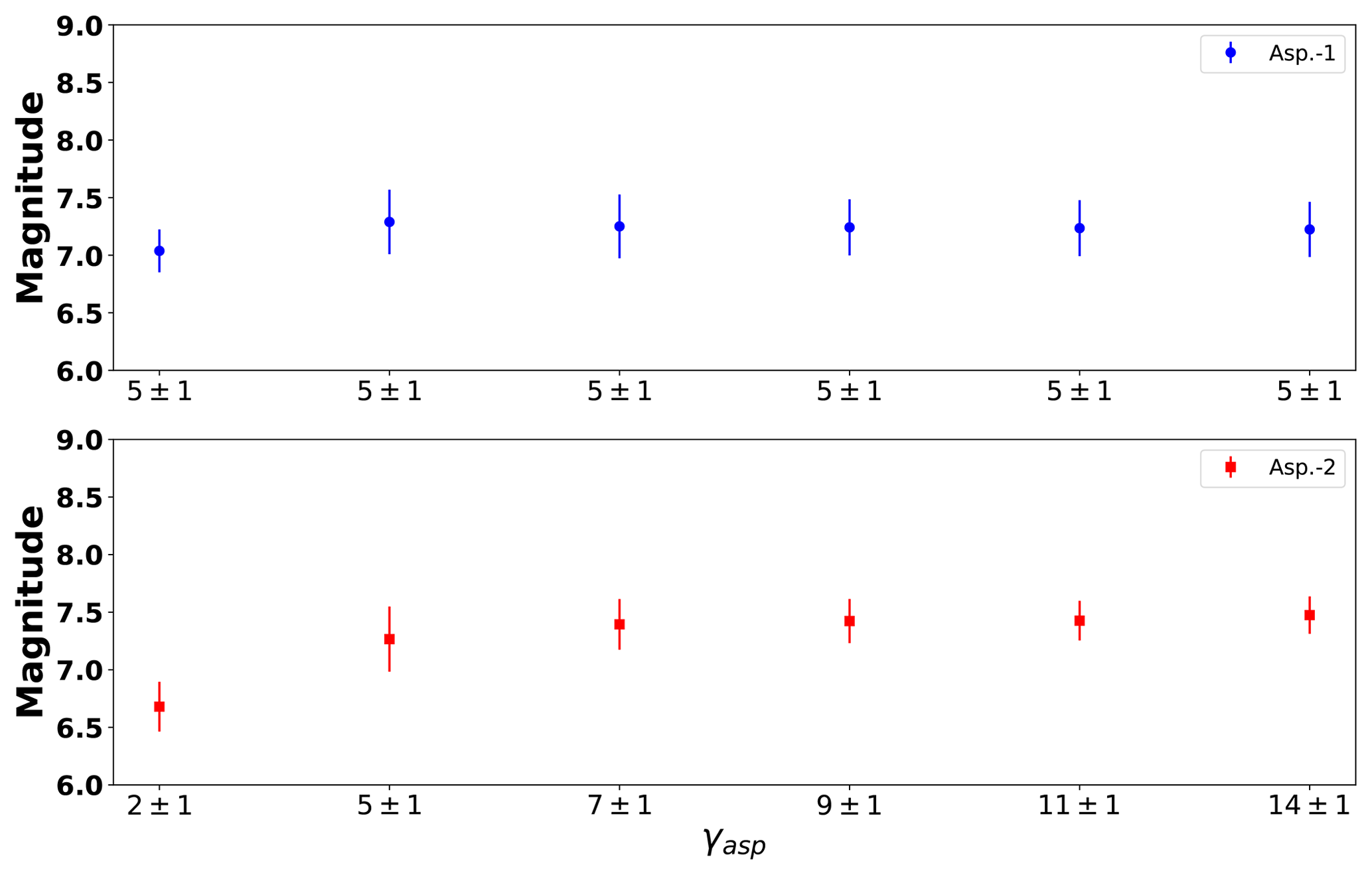
Figure 12Statistical results of γasp for a configuration similar to Fig. 6. Markers represent the mean value, while the error bars indicate the standard deviation for all 50 executions considering different initial strength configurations. The red markers correspond to the results of the left asperity (Asp. 1) and blue markers to the results of the right asperity (Asp. 2) (Fig. 6). The strength of the left asperity is kept constant, whereas the strength of the right asperity is variable.
We observe in Fig. 12 that the mean magnitude remains essentially independent for . Additionally, the error bars slightly decrease, while γasp increases. Another observation is that when the average of the maximum magnitude is the lowest in both asperities. Moreover, there is a transition zone for . We observed that has a limited influence on the results of the maximum magnitude. The maximum magnitude of is approximately 0.3 magnitudes larger than the one of .
5.1.3 Asperity size, Sa−Asp
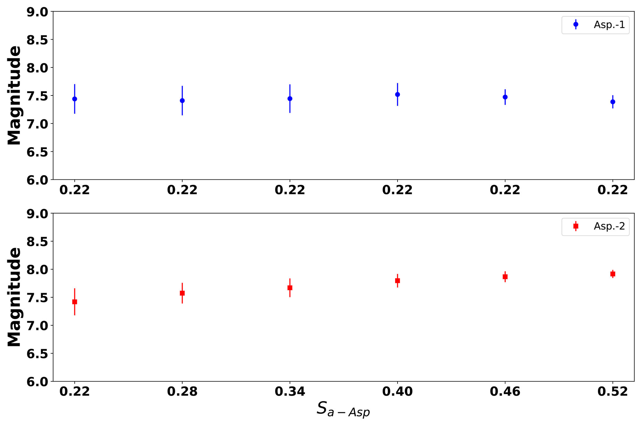
Figure 13 shows the mean magnitude and standard deviation as a function of asperity size. The first asperity with the fixed size indicates a relatively constant magnitude of approximately 7.4. Conversely, the second asperity with variable size produces only a slight increase in magnitude. The magnitude of is approximately 0.5 magnitudes larger than the one of .
5.2 Results: model validation
5.2.1 Modeling 10 Mexican subduction zone earthquakes
Based on the observations described in the previous section, we used and πasp=0.90 in order to validate the model. We chose because it represents the strength interval of with less computational cost. We chose πasp=0.90 because it represents the relatively constant magnitude for the parameter range . In addition, πasp=0.90 enables us to obtain the best approximation to the ratios of Sa−Asp. Both parameter choices ensure an appropriate reproduction of the asperity rupture area, the maximum magnitude, and least computational payload.
Figure 14 depicts a comparison between the (real) asperity area Areal (Table 5) and the area of the largest simulated earthquake, Asyn. We plot the mean (blue dots), the minimum (green triangles), and the maximum (red triangles) of all 50 realizations for each real earthquake event. Black squares represent the real asperity size. The results in Fig. 14 point out that Asyn is almost identical to Areal from Table 5 for the majority of earthquakes. Only three events show significant differences between synthetic and realistic maximum rupture area. Even in these cases, however, Areal is located within the upper and lower limit of Asyn.
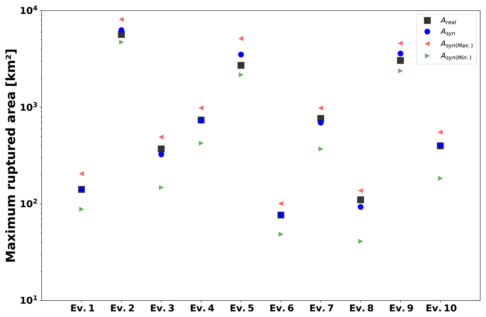
Figure 14Comparison between the real asperity area Areal and the synthetic values (mean and standard deviation) of the largest ruptured event Asyn. Black squares depict the real asperity area from Table 5, whereas blue circles indicate the mean area of 50 executions. Red and green triangles represent the maximum and minimum Asyn.
Figure 15 shows the statistical results of the synthetic maximum magnitude, Msyn, determined for all 10 events. The real magnitudes from Table 5 are given as red markers. Black circles indicate the mean of Msyn of 50 realizations using Eq. (7), whereas blue and green markers indicate the magnitude following the Eqs. (8) and (9), respectively. The error bars represent the standard deviation. We observed that the statistical parameters computed with TREMOL fit the magnitudes shown in Table 5. However, the computed magnitudes depend on the scale relation employed (Eqs. 7, 8, and 9). Figure 16 includes the mean of the three scale relations. Overall, the mean magnitude and the expected magnitude Mw show similar values. Given that the difference between the mean and the expected value (Table 5) is lower than ΔMw<0.5 for the 10 events, we can confirm that the results of assessing the magnitude by means of TREMOL using a randomly modified asperity size, Sa−Asp (Eq. 17), are reasonable.
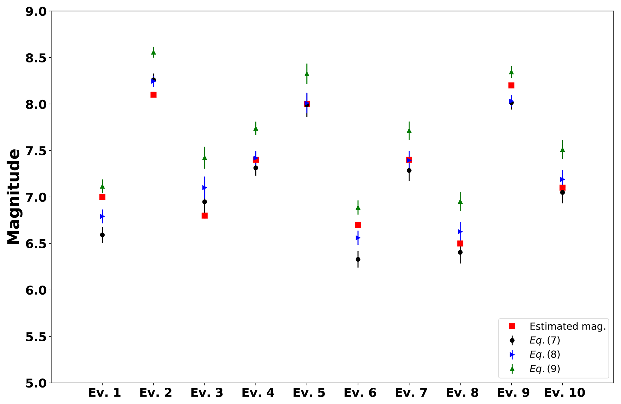
Figure 15Statistical results of the maximum magnitude for the events from Table 5. Red squares depict the real estimated magnitudes from Table 5, while black circles, blue triangles, and green triangles represent the synthetic mean magnitude of 50 executions following Eqs. (7), (8), and (9), respectively. The error bars are the standard deviation of the scale relations.

Figure 16Statistical results of the maximum magnitude for the events from Table 5. Red squares represent the magnitudes from Table 5, whereas black circles represent the mean magnitude () value of all 50 executions following Eqs. (7), (8), and (9). The error bars stand for the standard deviation of the mean for the three scale relations.
Figure 17 shows the real ratio size Sa from Table 5 (black squares) in comparison to the mean of the largest simulated earthquake, Ssyn (blue squares). The standard deviation is represented as error bars. The results indicate that in most of the cases the computed Ssyn range fits the expected Sa well. Note that for events 3, 7, and 8 the mean values are lower than the reported Sa, while Ssyn is overestimated for events 2, 5, and 9. For events 1, 4, 6, and 10 the estimated value of Ssyn coincides with the expected one. However, the error bars encompass the expected values in all cases (Fig. 17). Moreover, if we compare Fig. 17 with Fig. 11 we observe that the employed strategy of randomly increasing asperity size (using Eq. 17) generates rupture areas similar to the ones proposed by Rodríguez-Pérez et al. (2018).
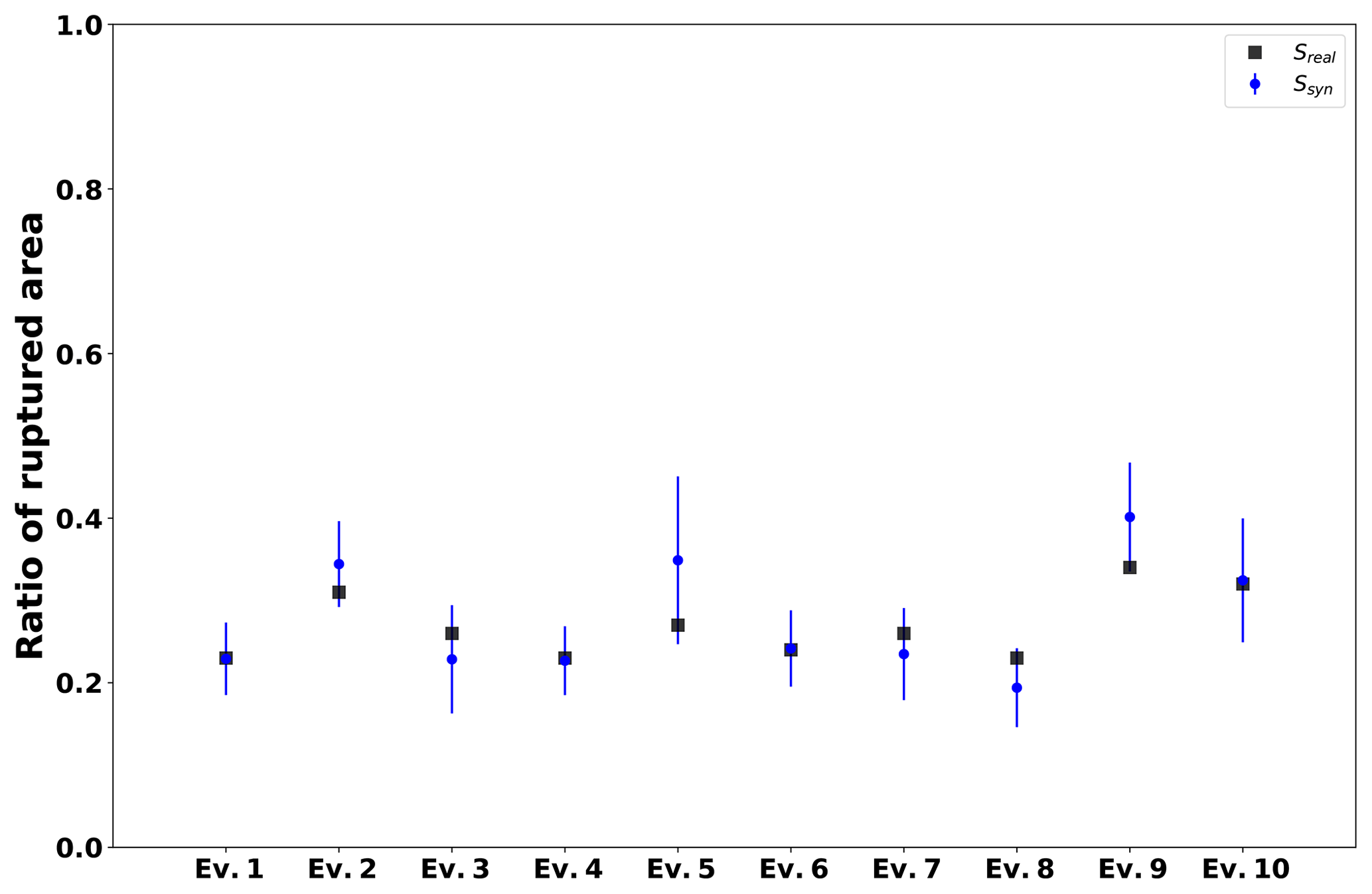
Figure 17Proportion of simulated ruptured area occupied by the largest avalanche, Ssyn, in comparison with the real ratio size Sa from Table 5. The real ratio size Sa from Table 5 is represented by black squares and the mean of the largest simulated earthquake, Ssyn, by blue squares. The standard deviation is represented as error bars.
We also computed an equivalent rupture duration, DAval, using the equation proposed by Geller (1976) to calculate the rise time (Eqs. 13 and 14). Rodríguez-Pérez and Ottemöller (2013) determined the rupture velocity Vr (Ev. 3–8), which is a useful parameter in order to validate our results. Figure 18 shows the results of this analysis. In red we plot the values Vr calculated by Rodríguez-Pérez and Ottemöller (2013) and in blue the DAval based on Eq. (13) with Vr provided by Table 5. The equivalent DAval using Eqs. (13) and (14) is printed in black. In cases in which we have the reference values, Vr, computed by Rodríguez-Pérez and Ottemöller (2013), we observe that the reference values are always larger than the modeled DAval values.
However, it is worth noting that Vr is the mean rupture time that considers the rupture of the whole effective area (Aeff). For the simulated rupture duration, DAval, we only consider the rupture length of the largest rupture cluster Asyn. As a result, smaller values than those proposed in Rodríguez-Pérez and Ottemöller (2013) are expected. Nevertheless, the rupture duration shows a clear dependency on the magnitude.

Figure 18Equivalent rupture duration DAval (s) calculated via the rupture velocity by using the size of the largest rupture cluster. Red squares represent the reference values proposed by Rodríguez-Pérez and Ottemöller (2013), while blue squares and black circles depict the synthetic rupture duration computed by means of Vr based on Eqs. (13) and (14), respectively.
5.2.2 Case study (Oaxaca, Mw=7.4, 20/03/2012)
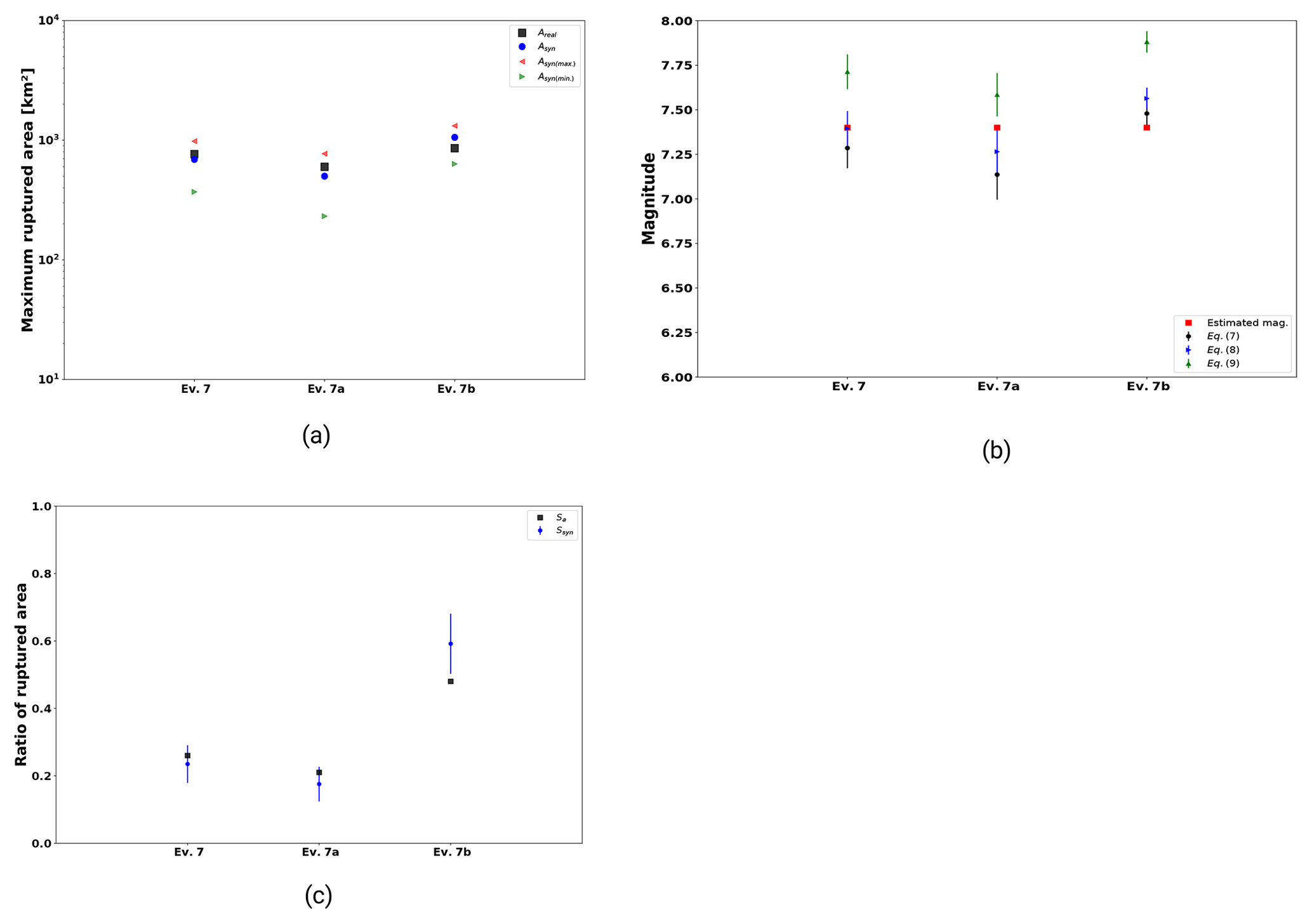
In the cases in which several effective rupture areas were proposed by different studies (see Table 5), it is possible to assess which set of parameters is better in order to simulate an event by means of TREMOL. We tested TREMOL by using three different combinations of Leff, Weff, and Sa according to results for Ev. 7 in Table 5. A comparison of these three combinations is visualized in Fig. 19: panel (a) shows the comparison of the ruptured areas, Areal and Asyn; panel (b) shows the mean and standard deviation of the maximum magnitude, Msyn, in comparison to the reference magnitude; and panel (c) shows the ratio Ssyn of the simulated events compared to Sa, the real scenarios. Although the three combinations express similar results, the closest approximation between real and synthetic data is generated based on Rodríguez-Pérez and Ottemöller (2013) (Ev. 7).
5.2.3 Assessing a future earthquake in the Guerrero seismic gap: rupture area and magnitude

In Fig. 20a, we compare the mean of maximum ruptured area, Asyn, including error bars with the reference area, Aa. The rupture area computed in TREMOL shows a possible range from 4000 to 7000 km2. This interval is based on a considered size of Sa=0.25. In the subplot of Fig. 20b, we estimated the duration Daval of the rupture event. The results in Fig. 20b indicate that the duration Daval is similar to that of the other events of magnitude Mw≈8. The duration may range from 80 to 110 s, while a rupture duration between 90 and 100 s is most likely. Figure 20c shows the mean of the estimated magnitude using Eqs. (7), (8), and (9). TREMOL outputs a possible range of , which matches the proposed value by Singh and Mortera (1991), Astiz et al. (1987), and Astiz and Kanamori (1984) of .
6.1 Discussion: parametric study
6.1.1 Percentage of transferred load, πasp
In the results, there were two dominant tendencies visible: (1) πasp<0.76 and (2) 0.76≤πasp. If πasp<0.76 the mean of the maximum ruptured area increased continuously more than 1 order of magnitude from 15 to ≈500 km2, i.e., an increase of 3333 %. Therefore, the range of πasp is both crucial and sensitive. A parameter increase of only 15 % affects the size of the biggest earthquake within the system by 3333 %. Considering the large standard deviation of ≈35 km2 (100 % error) a parameter configuration based on πasp<0.76 would be unsuitable for further simulations due to the unstable properties obtained for that range. The second tendency, however, offers the possibility to determine a stable conservation parameter that can be freely chosen in the range of . The stable state of maximum rupture area is caused by a self-organized critical avalanche size of Acrit≈500km2 based on a grid of 100×100 cells with Aeff=2944.2 km2 and Sa=0.26. As soon as Acrit is achieved by the system, the largest avalanche will stop increasing in size, whereas other avalanches within the system will be favored to grow. On the other hand, this means that TREMOL breaks the asperity in patches rather than completely during one unique rupture event (see Figs. 4 and 11). This last condition is reasonable considering that the algorithm of FBM used in TREMOL favors clustering the rupture of cells. Therefore, it is reasonable that some cells remain outside of a unique rupture group because they do not satisfy the failure conditions. As a consequence, we think that it is necessary to define an initial area greater than the expected area of the asperity where the asperity rupture can occur. This result also justifies the proposed Eq. (17), wherein the size of the asperity increases randomly up to 50 % larger than the value proposed by Rodríguez-Pérez et al. (2018). Future studies may be useful to better determine the influence of Acrit.
The parametric study indicates that the largest rupture πasp is produced as long as it is within the range . So even though as πasp increases, large rupture clusters are generated because a large amount of load is transferred to the neighboring cells, thereby producing critical local load concentrations in the system, the particular lower bound is critical. In our simulation short-range interactions convert to long-range processes through the avalanche mechanism in TREMOL v0.1. The explicit interaction range is given by the parameter π and the local load sharing rule, since this produces a load concentration in neighboring cells, promoting ruptures in a local manner (short range). However, the long range is also captured in a more implicit way.
As mentioned in Sect. 3.2, the algorithm searches for a cell to fail that fulfills two different criteria based on the stress and the strength values of the cells. This property results in long-range interactions since the randomness of the initial stress distribution allows cells at large distances to be activated after a sufficient amount of subsequent steps.
6.1.2 Strength parameter, γasp
The parameter γasp quantifies the “hardness” of the asperity in comparison to the background material. Its value is given as . The value γref=2 indicates that the strength in the asperity is twice as big as in the background area. The explored range of γref (2, 5, 7, 9, 11, 14) is based on an experimental trial. Figure 12 presents the mean of the maximum magnitude of an event as a function of γasp with two tendencies being visible.
-
There is an unstable transition zone of where the maximum rupture has a strong variation. Therefore, a strength value within this range should be avoided.
-
There is a stable zone of , where γasp can be freely chosen. However, due to computational costs it is recommended to use the lowest value of , since the number of necessary time steps to activate the whole asperity increases strongly with the applied asperity strength (see Algorithm 1).
Moreover, as γasp increases the simulation requires a larger number of iterations to break a cell in the asperity, thus implying a larger computational cost. Our selection (γref=5) ensures a “stable” maximum magnitude in the lowest computational time. Figure 21 visualizes the magnitude, the number of steps required to activate the whole asperity, and the computational time in seconds for one execution as a function of γref. In this sense, we considered a value of γref=5 to be adequate from a computational point of view and also to ensure relatively constant values of maximum magnitude.
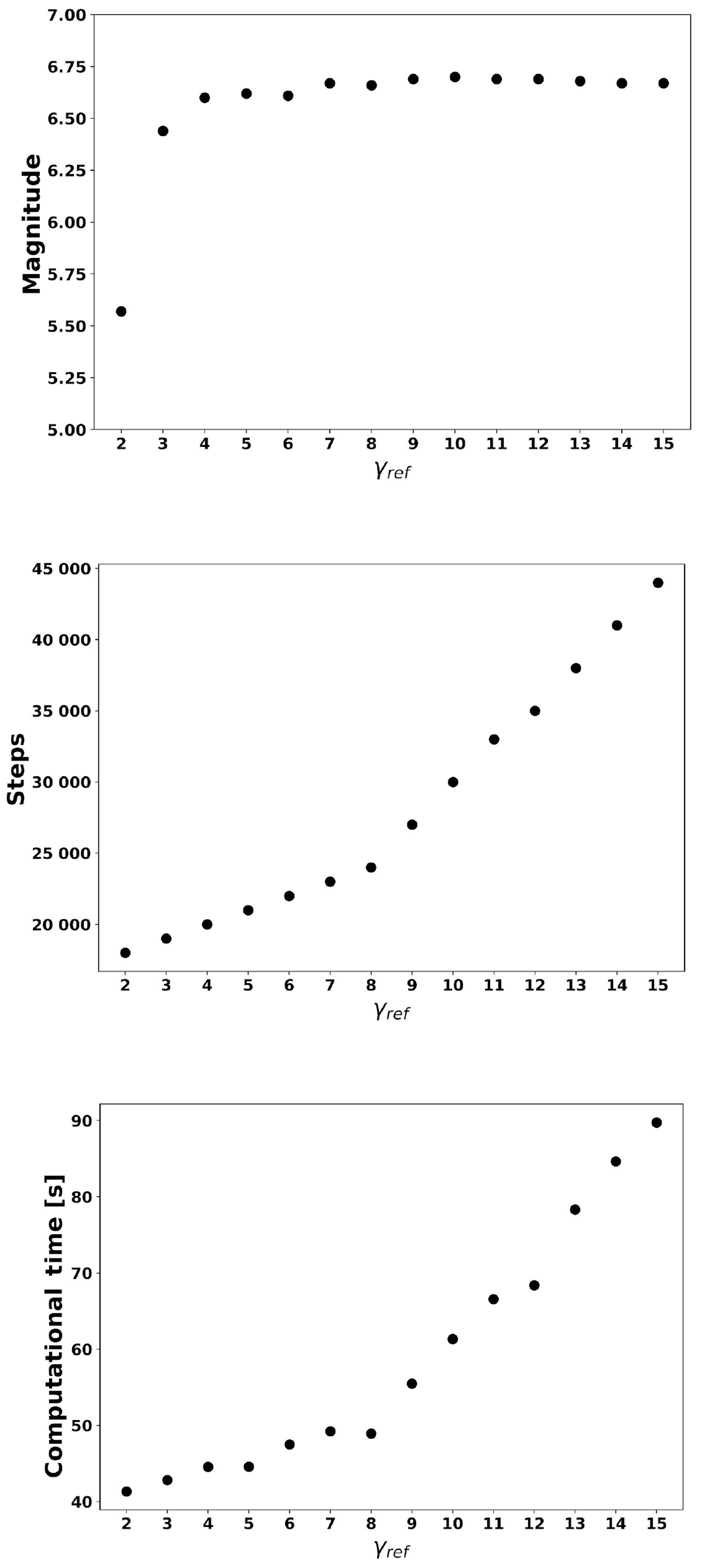
Figure 21Magnitude, computational time (s), and number of steps to “activate” the whole asperity for one execution as a function of γref.
6.1.3 Asperity size, Sa−Asp
The results of Fig. 13 indicate that asperity size has a significant influence on the maximum magnitude. We emphasize the importance of these results because they show that the parameter Sa−Asp is critical to control the generated magnitude. At the same time, these results provide the appropriate range of values that TREMOL requires to do a reasonable assessment of the maximum rupture area and magnitude of an earthquake.
6.2 Discussion: model validation
The model validation by means of 10 different subduction earthquakes showed that TREMOL is capable of reproducing rupture area and magnitude appropriately – by means of only few input data – in comparison to the results from inversion studies. The computed rupture duration by TREMOL differs from the reference values. The reason may be that the calculation of the rupture duration is based on the largest (critical) rupture area that is not equal to the available asperity area (see Figs. 11 and 6.1.1). Nevertheless, the rupture duration shows a clear dependency on the magnitude. Since TREMOL only requires few input data, it is a powerful tool to simulate future earthquakes, such as those that might take place in the Guerrero gap region. The determination of the magnitude of an earthquake based on the asperity area depends on the scale relation used. We considered it more appropriate that the relation used be related to the tectonic regime to be modeled. For example, other possible relations to be applied for a subduction earthquake regimen could be Strasser et al. (2010) and Blaser et al. (2010). However, if the user wants to include another empirical relation it is possible to add it in the script TREMOL_singlets/postprocessing/calcuMagniSpaceTime Singlets.jl, such as in the example presented by Wells and Coppersmith (1994). It is worth mentioning that the relation proposed by Wells and Coppersmith (1994) was analyzed as part of our tests. However, we found that the magnitude values are lower than the ones reported by Eqs. (7), (8), and (9). Blaser et al. (2010) discussed similarities and differences with Wells and Coppersmith (1994) in detail. Nevertheless, the rupture area is not model sensitive (Fig. 14), so in order to compare real data and simulations it is more appropriate to use the rupture area.
After validating the capability of the model, constraining the input parameters, and analyzing the results, we consider the conceptual basis of TREMOL to be expandable to model other tectonic regimes. For example, the FBM may be applied to study the rupture process in active fault systems and its effect on aftershock production. Likewise, a three-dimensional version can be developed to simulate mainshock rupture and its aftershocks as reported in Scholz (2018), who tested a first prototype of a 3-D version.
6.3 TREMOL: advantages and disadvantages
The algorithm of TREMOL enables the model to store stress history and to simulate static fatigue due to an included strength parameter γ. The vast majority of asperity parameters have already been examined in previous inversion studies and are usually accessible from online databases.
The range of values found in the sensitivity analysis are not unique for the Mexican examples. In fact, the parameters π, γ, and σ are generic for any simulation of similar types of earthquakes. The only information that needs to be defined beforehand for a unique earthquake is the effective area size and the asperity area, which may come from finite-fault models.
Dynamic deterministic modeling of aftershock series is still a challenge due to both the physical complexity and uncertainties related to the current state of the system. In seismicity process simulations the lack of knowledge of some important features, such as the initial stress distribution or the strength and material heterogeneities, generates a wide spectrum of uncertainties. One way to address this issue may be to consider a simple distribution such as a uniform distribution. We think that the validity of this assumption is given by the comparison of the simulated results with real data. It is possible that other distributions might also give similar results. However, the intention of TREMOL v0.1 is to propose a model that can be used to assign values to the unknown properties mentioned before, including different distributions. Therefore, we encourage users to try other distributions and investigate their effects.
The FBM, on the other hand, produces similar statistical and fractal characteristics as real earthquake series, and its parameters can be regarded as analogous to physical variables. Likewise, the FBM is able to simulate failure through static fatigue, creep failure, or delayed rupture (Pradhan and Chakrabarti, 2003; Moreno et al., 2001).
One disadvantage of TREMOL is that its output is highly dependent on the input, which is based on information from kinematic models and therefore contains inherent uncertainties from inversion studies (see Table 5). TREMOL may be able to compensate for some errors, but how far this possibility can be exploited needs to be investigated in the future. Further steps in the advance of the model have just started, which includes the analysis of a machine-learning approach (Monterrubio-Velasco et al., 2018) that will exploit all the possibilities of this technique.
There are still issues that will likely be addressed in future tests, as outlined below.
-
For our validations, we used earthquakes for which a suitable amount of information is available. How can the technique be applied to other events for which little information is available through, for instance, far-field recordings of seismicity?
-
For our validation study, we used a simplified geometry of the real complex asperity geometries. However, other irregular asperity geometries may be introduced in future works.
-
The FBM is a pure statistical model and therefore gives only hints about underlying physical processes. So far, it does not take into consideration physical effects such as pore fluid pressure, soil amplification, stress relaxation of the upper mantle, reactivation of existing faults, volcanic activity, and many more. One strength of the FBM is that an endless number of information layers can be included into the model that would allow us to include physical properties and topography as well.
-
As it currently stands, TREMOL is not able to simulate complete seismic cycles. Rate-and-state friction models such as by Lapusta et al. (2000) and Lapusta and Rice (2003) have the ability to reload stress. TREMOL is still in an early stage of development and thus lacks a reloading feature.
Additional setbacks of TREMOL are that (1) the number of time steps needs to be adjusted manually for every grid resolution and case scenario, and (2) it is based on a sequential algorithm. In order to save the stress history within every cell of the system, a consecutive algorithm is necessary that changes the state of the system with every time step. This limits the integration of a parallel domain, but a parallel distributed memory is a good approach to solve the problem of large domains. As a result high-performance computing facilities are required when very large grid sizes are used (Monterrubio-Velasco et al., 2018).
Overall, the results of TREMOL are promising. However, the results also point out the need for further modifications of the algorithm and more intensive studies. Likewise, many questions are still left to be answered due to the model's early development stage. In the very near future, however, TREMOL may be a true alternative to classical approaches in seismology. The simple integration of layers of information makes TREMOL a simple model that can be easily modified to simulate the most complex scenarios. At the moment, TREMOL cannot compete with state-of-the-art and widely accepted rate-and-state friction-based models, but it is a totally different, complementary, and promising approach that can provide important insights into earthquake physics and hazard assessment from a completely different perspective. The development of TREMOL and similar models should therefore be strongly encouraged and supported.
In this study, we present an FBM-based computer code called the stochasTic Rupture Earthquake MOdeL, TREMOL, in order to investigate the rupture process of seismic asperities. We show that the model is capable of reproducing the main characteristics observed in real scenarios by means of few input parameters. We carried out a parametric study in order to determine the optimal values for the three most important initial input parameters.
-
πasp. as long as the fault plane has a conservation parameter of πbkg=0.67, the conservation parameter of the asperity must be πasp≥0.76 to ensure a realistic maximum rupture area.
-
γasp. the best strength interval for the asperity is . However, due to computational costs it is recommended to use the lowest value of , since the number of necessary time steps to activate the whole asperity increases strongly with the applied asperity strength (see Algorithm 1).
-
Sa−Asp. the generated magnitude can be controlled by parameter Sa−Asp. This parameter is dependent on the earthquake of interest and follows results with data from inversion studies.
We also carried out a validation study employing 10 subduction earthquakes that occurred in Mexico. TREMOL proved that it is able to reproduce those scenarios with an appropriate tolerance.
A big advantage of our algorithm is the low number of free parameters (Leff, Weff, and Sa) to obtain an appropriate rupture area and magnitude assessment. Our code TREMOL allows its users to investigate the role of the initial stress configuration and the material properties over the seismic asperity rupture. Both characteristics are key factors for understanding earthquake dynamics. The strengths of our FBM model are the simplicity of implementation, the flexibility, and the capability to model different rupture scenarios (i.e., asperity configurations) with varying mechanical properties within the asperities and/or background area or fault plane. Although we simplified the expected complex asperity geometries, irregular asperity geometries may be introduced in future works. Another advantage is the analysis of earthquake dynamics from the point of view of deformable materials that break under critical stress. The results of TREMOL are promising. However, various assumptions and simplifications require further experiments and modifications of the algorithm to cover various tectonic settings. Likewise, the machine-learning application by Monterrubio-Velasco et al. (2018) needs to be incorporated into the model to determine the optimal parameter ranges for different fault types and tectonic regimes. Although many questions are still left to be answered due to the model's early development stage, TREMOL proved to be a powerful tool that can deliver promising new insights into earthquake triggering processes. Our future work will investigate complex asperity configurations, earthquake doublets, and stress transfer in three-dimensional domains.
The TREMOL code is freely available at the home page (https://doi.org/10.5281/zenodo.1884981, Monterrubio-Velasco, 2018b), from its GitHub repository (https://github.com/monterrubio-velasco), or by request to the author (marisol.monterrubio@bsc.es, marisolmonterrub@gmail.com). In all cases, the code is supplied in a manner to ease the immediate execution under Linux platforms. User's manual documentation is provided in the archive as well.
MMV developed the code TREMOL v0.1. MMV, QRP, RZ, AAM, and JP provided guidance and theoretical advice during the study. All the authors contributed to the analysis and interpretation of the results. DS helped in the improving of the paper's style and the user manual. All the authors contributed to the writing and editing of the paper.
The authors declare that they have no conflict of interest.
The authors are grateful to two anonymous reviewers and the editor for their relevant and constructive comments that have greatly contributed to improving the paper. M. Monterrubio-Velasco and J. de la Puente thank the European Union's Horizon 2020 Programme under the ChEESE Project (https://cheese-coe.eu/, last access: 1 May 2019), grant agreement no. 823844, for partially funding this work. M. Monterrubio-Velasco and A. Aguilar-Meléndez thank CONACYT for support of this research project. Quetzalcoatl Rodríguez-Pérez was supported by the Mexican National Council for Science and Technology (CONACYT) (Catedras program, project 1126). This project has received funding from the European Union's Horizon 2020 research and innovation program under Marie Skłodowska-Curie grant agreement no. 777778, MATHROCKS, and from the Spanish Ministry project TIN2016-80957-P. Initial funding for the project through grant UNAM-PAPIIT IN108115 is also gratefully acknowledged.
This paper was edited by Thomas Poulet and reviewed by two anonymous referees.
Andersen, J. V., Sornette, D., and Leung, K.-T.: Tricritical behavior in rupture induced by disorder, Phys. Rev. Lett., 78, 2140–2143, https://doi.org/10.1103/PhysRevLett.78.2140, 1997. a
Aochi, H. and Ide, S.: Conceptual multi-scale dynamic rupture model for the 2011 off the Pacific coast of Tohoku Earthquake, Earth Planet. Space, 63, 761–765, https://doi.org/10.5047/eps.2011.05.008, 2011. a
Astiz, L. and Kanamori, H.: An earthquake doublet in Ometepec, Guerrero, Mexico, Phys. Earth Planet. In., 34, 24–45, 1984. a, b
Astiz, L., Kanamori, H., and Eissler, H.: Source characteristics of earthquakes in the Michoacan seismic gap in Mexico, B. Seismol. Soc. Am., 77, 1326–1346, 1987. a, b
Bak, P. and Tang, C.: Earthquakes as a self-organized critical phenomenon, J. Geophys. Res.-Sol. Ea., 94, 15635–15637, 1989. a, b, c
Barriere, B. and Turcotte, D.: Seismicity and self-organized criticality, Phys. Rev. E, 49, 1151–1160, https://doi.org/10.1103/PhysRevE.49.1151, 1994. a, b
Biswas, S., Ray, P., and Chakrabarti, B. K.: Statistical physics of fracture, breakdown, and earthquake: effects of disorder and heterogeneity, John Wiley & Sons, USA, 2015. a
Blaser, L., Krüger, F., Ohrnberger, M., and Scherbaum, F.: Scaling relations of earthquake source parameter estimates with special focus on subduction environment, B. Seismol. Soc. Am., 100, 2914–2926, 2010. a, b
Caruso, F., Pluchino, A., Latora, V., Vinciguerra, S., and Rapisarda, A.: Analysis of self-organized criticality in the Olami-Feder-Christensen model and in real earthquakes, Phys. Rev. E, 75, 055101, https://doi.org/10.1103/PhysRevE.75.055101, 2007. a
Chakrabarti, B. K. and Benguigui, L.-G.: Statistical physics of fracture and breakdown in disordered systems, vol. 55, Oxford University Press, UK, 1997. a
Coleman, B. D.: Statistics and time dependence of mechanical breakdown in fibers, J. Appl. Phys., 29, 968–983, 1958. a
Daniels, H. E.: The statistical theory of the strength of bundles of threads, I, Proc. R. Soc. Lond. A, 183, 405–435, 1945. a
Das, S. and Aki, K.: Fault plane with barriers: a versatile earthquake model, J. Geophys. Res., 82, 5658–5670, 1977. a
Das, S. and Kostrov, B.: Fracture of a single asperity on a finite fault: a model for weak earthquakes?, Earthq. Source Mech., 37, 91–96, 1986. a
Eshelby, J. D.: The determination of the elastic field of an ellipsoidal inclusion, and related problems, Proc. R. Soc. Lond. A, 241, 376–396, 1957. a
Geller, R. J.: Scaling relations for earthquake source parameters and magnitudes, B. Seismol. Soc. Am., 66, 1501–1523, 1976. a, b
Gómez, J., Moreno, Y., and Pacheco, A.: Probabilistic approach to time-dependent load-transfer models of fracture, Phys. Rev. E, 58, 1528–1523, https://doi.org/10.1103/PhysRevE.58.1528, 1998. a, b
Hansen, A., Hemmer, P. C., and Pradhan, S.: The fiber bundle model: modeling failure in materials, John Wiley & Sons, USA, 2015. a, b
Iwata, T. and Asano, K.: Characterization of the heterogeneous source model of intraslab earthquakes toward strong ground motion prediction, Pure Appl. Geophys., 168, 117–124, 2011. a, b
Kanamori, H. and Stewart, G. S.: Seismological aspects of the Guatemala earthquake of February 4, 1976, J. Geophys. Res.-Sol. Ea., 83, 3427–3434, 1978. a
Kloster, M., Hansen, A., and Hemmer, P. C.: Burst avalanches in solvable models of fibrous materials, Phys. Rev. E, 56, 2615–2625, https://doi.org/10.1103/PhysRevE.56.2615, 1997. a
Kun, F., Hidalgo, R. C., Raischel, F., and Herrmann, H. J.: Extension of fibre bundle models for creep rupture and interface failure, Int. J. Frac., 140, 255–265, 2006a. a
Kun F., Raischel F., Hidalgo R., and Herrmann H.: Extensions of Fibre Bundle Models. In: Modelling Critical and Catastrophic Phenomena in Geoscience, edited by: Bhattacharyya P. and Chakrabarti B. K., Lecture Notes in Physics, vol 705, Springer, Berlin, Heidelberg, https://doi.org/10.1007/3-540-35375-5_3, 2006b. a
Lapusta, N. and Rice, J.: Nucleation and early seismic propagation of small and large events in a crustal earthquake model, J. Geophys. Res.-Sol. Ea., 108, 1–18, 2003. a
Lapusta, N., Rice, J. R., Ben-Zion, Y., and Zheng, G.: Elastodynamic analysis for slow tectonic loading with spontaneous rupture episodes on faults with rate-and state-dependent friction, J. Geophys. Res.-Sol. Ea., 105, 23765–23789, 2000. a
Lee, M. and Sornette, D.: Novel mechanism for discrete scale invariance in sandpile models, Eur. Phys. J. B, 15, 193–197, 2000. a
Madariaga, R.: On the relation between seismic moment and stress drop in the presence of stress and strength heterogeneity, J. Geophys. Res.-Sol. Ea., 84, 2243–2250, 1979. a, b
Mai, P. M. and Beroza, G. C.: Source scaling properties from finite-fault-rupture models, B. Seismol. Soc. Am., 90, 604–615, 2000. a
Mai, P. M., Spudich, P., and Boatwright, J.: Hypocenter locations in finite-source rupture models, B. Seismol. Soc. Am., 95, 965–980, 2005. a, b
Mendoza, C. and Hartzell S. H.: Slip distribution of the 19 September 1985 Michoacán, México, earthquake: near source and teleseismic contraints, Bull. Seismol Soc. Am., 79, 655–669, 1989. a
Monterrubio, M., Lana, X., and Martínez, M. D.: Aftershock sequences of three seismic crises at southern California, USA, simulated by a cellular automata model based on self-organized criticality, Geosci. J., 19, 81–95, 2015. a
Monterrubio-Velasco, M., Zúñiga, F., Márquez-Ramírez, V. H., and Figueroa-Soto, A.: Simulation of spatial and temporal properties of aftershocks by means of the fiber bundle model, J. Seismol., 21, 1623–1639, 2017. a, b, c
Monterrubio-Velasco, M., Carrasco-Jiménez, C., Castillo-Reyes, O., Cucchietti, F., and la Puente J., D.: A Machine Learning Approach for Parameter Screening in Earthquake Simulation, in: High Performance Machine Learning Workshop, 24–27 September, Lyon, France, https://doi.org/10.1109/CAHPC.2018.8645865, 2018a. a, b, c
Monterrubio-Velasco, M.: TREMOL_singlets, Zenodo, https://doi.org/10.5281/zenodo.1884981, 2018b.
Moral, L., Moreno, Y., Gómez, J., and Pacheco, A.: Time dependence of breakdown in a global fiber-bundle model with continuous damage, Phys. Rev. E, 63, 066106, https://doi.org/10.1103/PhysRevE.63.066106, 2001. a, b
Moreno, Y., Correig, A., Gómez, J., and Pacheco, A.: A model for complex aftershock sequences, J. Geophys. Res.-Sol. Ea., 106, 6609–6619, 2001. a, b, c, d, e, f, g
Murotani, S., Miyake, H., and Koketsu, K.: Scaling of characterized slip models for plate-boundary earthquakes, Earth Planet. Space, 60, 987–991, 2008. a, b, c
Olami, Z., Feder, H., S., J., and Christensen, K.: Comparison of average stress drop measures for ruptures with heterogeneous stress change and implications for earthquake physics, Phys. Rev. Lett., 68, 1244, https://doi.org/10.1103/PhysRevLett.68.1244, 1992. a, b
Peirce, F. T.: Tensile tests for cotton yarns: “the weakest link” theorems on the strength of long and of composite specimens, J. Textile Inst., 17, 355–368, 1926. a
Phoenix, S. L.: Stochastic strength and fatigue of fiber bundles, Int. J. Frac., 14, 327–344, 1978. a
Phoenix, S. L. and Beyerlein, I.: Statistical strength theory for fibrous composite materials, Comprehens. Composite Mat., 1, 559–639, 2000. a
Phoenix, S. L. and Tierney, L.: A statistical model for the time dependent failure of unidirectional composite materials under local elastic load-sharing among fibers, Eng. Fract. Mech., 18, 193–215, 1983. a
Pradhan, S. and Chakrabarti, B. K.: Failure properties of fiber bundle models, Int. J. Modern Phys. B, 17, 5565–5581, 2003. a, b
Pradhan, S., Hansen, A., and Chakrabarti, B. K.: Failure processes in elastic fiber bundles, Rev. Modern Phys., 82, 499–555, https://doi.org/10.1103/RevModPhys.82.499, 2010. a
Rodríguez-Pérez, Q. and Ottemöller, L.: Finite-fault scaling relations in Mexico, Geophys. J. Int., 193, 1570–1588, 2013. a, b, c, d, e, f, g, h, i, j, k, l, m, n, o, p
Rodríguez-Pérez, Q. and Zúñiga, F.: Båth's law and its relation to the tectonic environment: A case study for earthquakes in Mexico, Tectonophysics, 687, 66–77, 2016. a
Rodríguez-Pérez, Q., Márquez-Ramírez, V., Zúñiga, F., Plata-Martínez, R., and Pérez-Campos, X.: The Mexican Earthquake Source Parameter Database: A New Resource for Earthquake Physics and Seismic Hazard Analyses in México, Seismol. Res. Lett., 89, 1846–1862, https://doi.org/10.1785/0220170250, 2018. a, b, c, d, e
Scholz, D. N.: Numerical simulations of stress transfer as a future alternative to classical Coulomb stress change? Investigation of the El Mayor Cucapah event, Master's thesis, University College London, London, 2018. a, b
Singh, S. and Mortera, F.: Source time functions of large Mexican subduction earthquakes, morphology of the Benioff zone, age of the plate, and their tectonic implications, J. Geophys. Res., 96, 21487–21502, 1991. a, b, c
Somerville, P., Irikura, K., Graves, R., Sawada, S., Wald, D., Abrahamson, N., Iwasaki, Y., Kagawa, T., Smith, N., and Kowada, A.: Characterizing crustal earthquake slip models for the prediction of strong ground motion, Seismol. Res. Lett., 70, 59–80, 1999. a, b, c, d, e
Somerville, P. G., Sato, T., Ishii, T., Collins, N., Dan, K., and Fujiwara, H.: Characterizing heterogeneous slip models for large subduction earthquakes for strong ground motion prediction, in: Proceedings of the 11th Japan Earthquake Engineering Symposium, 20–22 November, Tokio, vol. 1, 163–166, Architectural Institute of Japan, 2002. a, b
Stein, S. and Wysession, M.: An introduction to seismology, eartquakes, and Earth structure, John Wiley & Sons, USA, 2008. a
Strasser, F., Arango, M., and Bommer, J.: Scaling of the source dimensions of interface and intraslab subduction-zone earthquakes with moment magnitude, Seismol. Res. Lett., 81, 941–950, 2010. a
Turcotte, D. L. and Glasscoe, M. T.: A damage model for the continuum rheology of the upper continental crust, Tectonophysics, 383, 71–80, 2004. a
Vázquez-Prada, M., Gómez, J., Moreno, Y., and Pacheco, A.: Time to failure of hierarchical load-transfer models of fracture, Phys. Rev. E, 60, 2581–2594, https://doi.org/10.1103/PhysRevE.60.2581, 1999. a, b
Wells, D. L. and Coppersmith, K. J.: New empirical relationships among magnitude, rupture length, rupture width, rupture area, and surface displacement, B. Seismol. Soc. Am., 84, 974–1002, 1994. a, b, c
Yewande, O. E., Moreno, Y., Kun, F., Hidalgo, R. C., and Herrmann, H. J.: Time evolution of damage under variable ranges of load transfer, Phys. Rev. E, 68, 026116, https://doi.org/10.1103/PhysRevE.68.026116, 2003. a