the Creative Commons Attribution 4.0 License.
the Creative Commons Attribution 4.0 License.
 | 15 May 2019
CSIB v1 (Canadian Sea-ice Biogeochemistry): a sea-ice biogeochemical model for the NEMO community ocean modelling framework
Hakase Hayashida
James R. Christian
Amber M. Holdsworth
Xianmin Hu
Adam H. Monahan
Eric Mortenson
Paul G. Myers
Olivier G. J. Riche
Tessa Sou
Nadja S. Steiner
Process-based numerical models are a useful tool for studying marine ecosystems and associated biogeochemical processes in ice-covered regions where observations are scarce. To this end, CSIB v1 (Canadian Sea-ice Biogeochemistry version 1), a new sea-ice biogeochemical model, has been developed and embedded into the Nucleus for European Modelling of the Ocean (NEMO) modelling system. This model consists of a three-compartment (ice algae, nitrate, and ammonium) sea-ice ecosystem and a two-compartment (dimethylsulfoniopropionate and dimethylsulfide) sea-ice sulfur cycle which are coupled to pelagic ecosystem and sulfur-cycle models at the sea-ice–ocean interface. In addition to biological and chemical sources and sinks, the model simulates the horizontal transport of biogeochemical state variables within sea ice through a one-way coupling to a dynamic-thermodynamic sea-ice model (LIM2; the Louvain-la-Neuve Sea Ice Model version 2). The model results for 1979 (after a decadal spin-up) are presented and compared to observations and previous model studies for a brief discussion on the model performance. Furthermore, this paper provides discussion on technical aspects of implementing the sea-ice biogeochemistry and assesses the model sensitivity to (1) the temporal resolution of the snowfall forcing data, (2) the representation of light penetration through snow, (3) the horizontal transport of sea-ice biogeochemical state variables, and (4) light attenuation by ice algae. The sea-ice biogeochemical model has been developed within the generic framework of NEMO to facilitate its use within different configurations and domains, and can be adapted for use with other NEMO-based sub-models such as LIM3 (the Louvain-la-Neuve Sea Ice Model version 3) and PISCES (Pelagic Interactions Scheme for Carbon and Ecosystem Studies).
- Article
(12239 KB) -
Supplement
(225 KB) - BibTeX
- EndNote


Biogeochemical processes at the sea-ice–ocean interface play an active role in polar marine ecosystems and global cycling of important chemical elements and compounds. For example, microalgae that colonize the base of sea ice in spring can have a strong influence on primary production of phytoplankton through light attenuation, nutrient drawdown, and seeding as well as on secondary production by providing a food source for grazers (Arrigo, 2014). Furthermore, these ecological processes regulate the production and removal of greenhouse gases (e.g., carbon dioxide and nitrous oxide) and other climatically important gases (e.g., dimethylsulfide) in ice-covered regions, and the exchange of these gases with the overlying atmosphere (Vancoppenolle et al., 2013).
However, our current understanding of many of these processes remains limited due to both logistical and technical challenges for field observations (Miller et al., 2015). Process-based numerical models representing sea-ice biogeochemistry can both fill gaps between sparse measurements and aid in the interpretation of these measurements. Furthermore, these models can be used in systematic intercomparisons that can build confidence in our understanding of polar marine science such as has been done for pelagic ecosystem models (e.g., Popova et al., 2012; Jin et al., 2015).
Dupont (2012)Jin et al. (2012)Watanabe et al. (2015)Castellani et al. (2017)Table 1Comparison of pan-Arctic 3-D sea-ice biogeochemical model configurations developed in various frameworks. dx: the horizontal resolution; dzo: the vertical resolution of the uppermost water column; dzi: the vertical extent of the biologically active layer at ice base; i0 (snow surface): the fraction of incoming shortwave radiation that penetrates through the snow surface; Shading: attenuation of light by ice algae; Runoff: river discharge of nitrate.
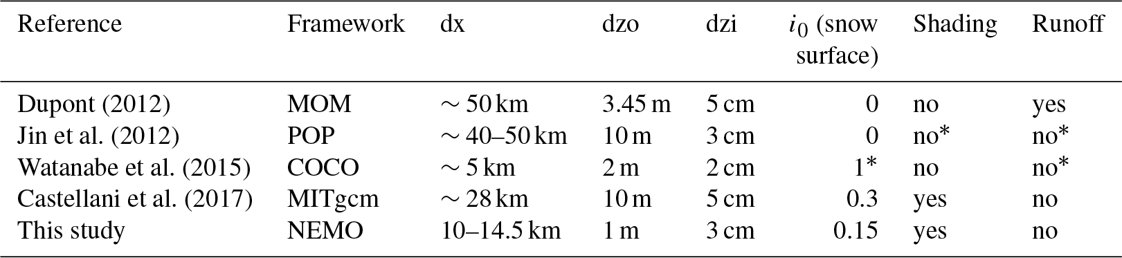
∗ Confirmed through personal communication with the lead author (2018).
Although considerable effort has been invested in developing process-based numerical models for sea-ice biogeochemistry over the last 3 decades following the pioneering work of Arrigo et al. (1991), most of these models were applied in one-dimensional (1-D) frameworks, and the results are therefore limited to particular locations (see Vancoppenolle and Tedesco, 2016). Only a few of these models have been applied in three-dimensional (3-D) framework coupled to either a regional or global sea-ice–ocean general circulation model (see Table 1 for a list of 3-D model configurations developed for pan-Arctic studies). More efforts toward developing such 3-D sea-ice biogeochemical models are needed to better understand the large-scale variability in biogeochemical processes within sea ice and their role in underlying pelagic and benthic ecosystems.
In this study, we present CSIB v1 (Canadian Sea-ice Biogeochemistry version 1), a new sea-ice biogeochemical model implemented into the Nucleus for European Modelling of the Ocean (NEMO), a state-of-the-art modelling framework for oceanographic research (https://www.nemo-ocean.eu/, last access: 13 May 2019). To the best of our knowledge, Tedesco et al. (2017) is the only previous study in which a sea-ice biogeochemical model has been coupled to NEMO. However, the coupling is done in an offline configuration in that study. An important advance of the present study is that the model is written within the NEMO code to allow in-line coupling (i.e., physical dynamics are computed simultaneously with biogeochemistry) and the computation of horizontal transport of sea-ice biogeochemical state variables associated with sea-ice drift. These implementations allow for more realistic simulation of sea-ice biogeochemistry and intercomparison of process-based numerical ice algae models. The main objectives of the present study are to describe the development of the coupled model in a pan-Arctic configuration (Sect. 2), present the basic features of the simulation (Sect. 3), and assess the model sensitivity to modifications of parameters and parameterizations (Sect. 4). Key findings of the present study are summarized in Sect. 5. We note that this study is intended as a model description paper, and the analysis focuses on results for the year 1979, corresponding to the end of a decadal model spin-up. The analysis of the simulation beyond 1979, in which more observational data are available for evaluation (Hayashida, 2018a), is planned to be published as a journal article separately.
The fundamental constituents of NEMO are the following three sub-models: ocean physics, sea-ice physics, and ocean biogeochemistry. In the present study, we adopted version 3.4 of NEMO (NEMO v3.4; Madec, 2008) and developed within it an additional sub-model, sea-ice biogeochemistry. Technical details on the code structure of the model developed in this study are provided in Appendix A for those who are interested in using the newly added sea-ice biogeochemical model.
2.1 Ocean and sea-ice physics (OPA–LIM2)
The physical ocean sub-model is the Océan PArallélisé (OPA), which is a free-surface, hydrostatic, primitive-equation model developed for regional and global ocean circulation studies (Madec, 2008). OPA is coupled to the sub-model for sea-ice physics, namely the Louvain-la-Neuve Sea Ice Model (LIM). The present study uses version 2 of LIM (LIM2; Fichefet and Maqueda, 1997; Bouillon et al., 2009), consisting of a three-layer (one for snow and two for ice) dynamic-thermodynamic model.
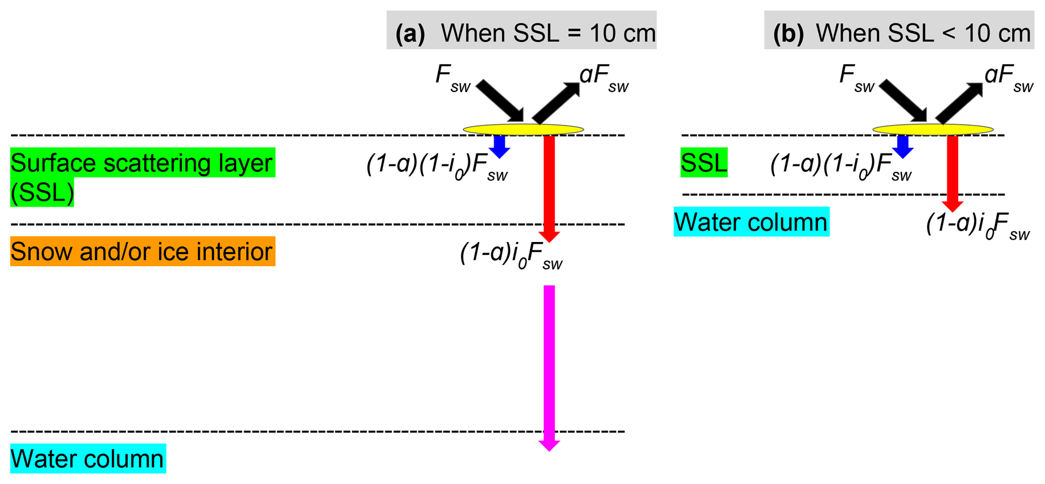
Figure 1Shortwave radiative transfer through snow and sea ice in the LIM2/LIM3 model. Fsw represents the incoming shortwave radiation, a fraction of which is reflected due to the surface albedo of snow or ice (a). The remaining radiation is either absorbed within the surface scattering layer (SSL) (; blue arrows) or penetrates below the SSL ((1−a)i0Fsw; red arrows). (a) When the SSL is 10 cm (i.e., the sum of snow depth and ice thickness is equal to or greater than 10 cm), the radiation penetrating into the snow and/or ice interior attenuates following the Beer–Lambert law and reaches the water column (magenta arrow). (b) When the SSL is less than 10 cm, the penetrating radiation directly reaches the water column. Modified from Fig. 3.4 of Vancoppenolle et al. (2012).
To model ambient light available for ice algae and under-ice phytoplankton properly, we modified the module that computes the shortwave radiative transfer through snow and sea ice as shown schematically in Fig. 1. In this module, the unreflected fraction (1−a) of the incoming shortwave radiation (Fsw) is parameterized as either being absorbed within a thin layer of surface snow and/or ice or penetrating below this layer. This thin layer at the surface is known as the surface scattering layer (SSL; Grenfell and Maykut, 1977), and is defined in the model as the uppermost 10 cm of snow and/or ice column in NEMO v3.4. When the sum of snow depth and ice thickness is less than 10 cm, the SSL equals this total thickness. The penetrating fraction is determined by the coefficient i0, which is set to zero in the presence of snow in the default configuration of LIM2 following Maykut and Untersteiner (1971). While this assumption of complete blockage of light may be a reasonable approximation for thermodynamic processes of snow and sea ice, it is problematic for modelling sea-ice biogeochemistry. Specifically, the assumption implies that primary producers can not photosynthesize until snow disappears completely, which is inconsistent with the findings of many field observations that measure high algal biomass at the base of snow-covered sea ice (e.g., Leu et al., 2015). Furthermore, i0 for snow surface has been set to non-zero values in other sea-ice models in the case of thin or melting snow (Flato and Brown, 1996; Abraham et al., 2015). For these reasons, we use a non-zero value of i0 for snow surface and parameterize the light transmission through the snow column below the specified surface layer following the Beer–Lambert law. The value of i0 for snow surface was set to 0.15 following the 1-D sea-ice biogeochemical modelling work of Vancoppenolle et al. (2010). The attenuation coefficient of snow was set to 10 m−1, which falls within the observed range for melting and freezing snow (Grenfell and Maykut, 1977). Model sensitivity to i0 for snow surface is discussed in Sect. 4.2.
2.2 Ocean biogeochemistry (CanOE)
The sub-model for ocean biogeochemistry adopted in the present study is the Canadian Ocean Ecosystem Model (CanOE), developed by the ocean modelling group at the Canadian Centre for Climate Modelling and Analysis (Christian et al., 2019; see Appendix A3 of Hayashida, 2018a). This model has been developed for the latest version of the Canadian Earth System Model (CanESM5), which will be used in the next phase of the Coupled Model Intercomparison Project (CMIP6). CanOE simulates the lower trophic levels of marine ecosystems (nutrients, phytoplankton, zooplankton, and detritus) and biogeochemical cycling of key elements (carbon, oxygen, nitrogen, and iron). This model is built around the basic code structure of the Pelagic Interactions Scheme for Carbon and Ecosystem Studies (PISCES) version 2, the default sub-model for ocean biogeochemistry of NEMO (Aumont et al., 2015). CanOE is an updated version of the Canadian Model of Ocean Carbon (CMOC) used in an earlier version of CanESM (CanESM2; Arora et al., 2011) designed to limit the complexity as much as possible, while addressing insufficiencies in CMOC (e.g., single nutrient–phytoplankton–zooplankton–detritus models are either tuned towards low-nutrient or high-nutrient conditions). CanOE is somewhat more efficient than PISCES as a result of having fewer state variables (19 vs. 24) and fewer computationally expensive parameterizations (Christian et al., 2019; Appendix A3 of Hayashida, 2018a).
In the present study, we made two modifications to CanOE. The first modification is the addition of an ocean sulfur-cycle model and the second modification is the parameterization of the photosynthetically active radiation (PAR).
2.2.1 Addition of an ocean sulfur cycle
Figure 2 shows a schematic of CanOE including the ocean sulfur cycle and the sea-ice biogeochemistry. Here, the sulfur cycle is restricted to sources and sinks of two state variables: dissolved dimethylsulfoniopropionate (DMSPd) and dimethylsulfide (DMS). The ocean sulfur cycle is one-way coupled to CanOE as the sources and sinks of DMSPd and DMS depend on the conditions of primary and secondary producers, but not vice versa. The ocean sulfur-cycle model is based on Hayashida et al. (2017) with the following two modifications. First, the cellular DMSP content of modelled phytoplankton is derived from their carbon content as opposed to the chlorophyll content as in Hayashida et al. (2017). This change was made because there are more observation-based estimates of the intracellular DMSP-to-carbon (DMSP to C) ratio than the DMSP-to-chlorophyll a ratio (e.g., Stefels et al., 2007). The DMSP:C ratios for small and large phytoplankton (respectively high and low DMSP producers) are set to 12 and 4 mmol mol−1.
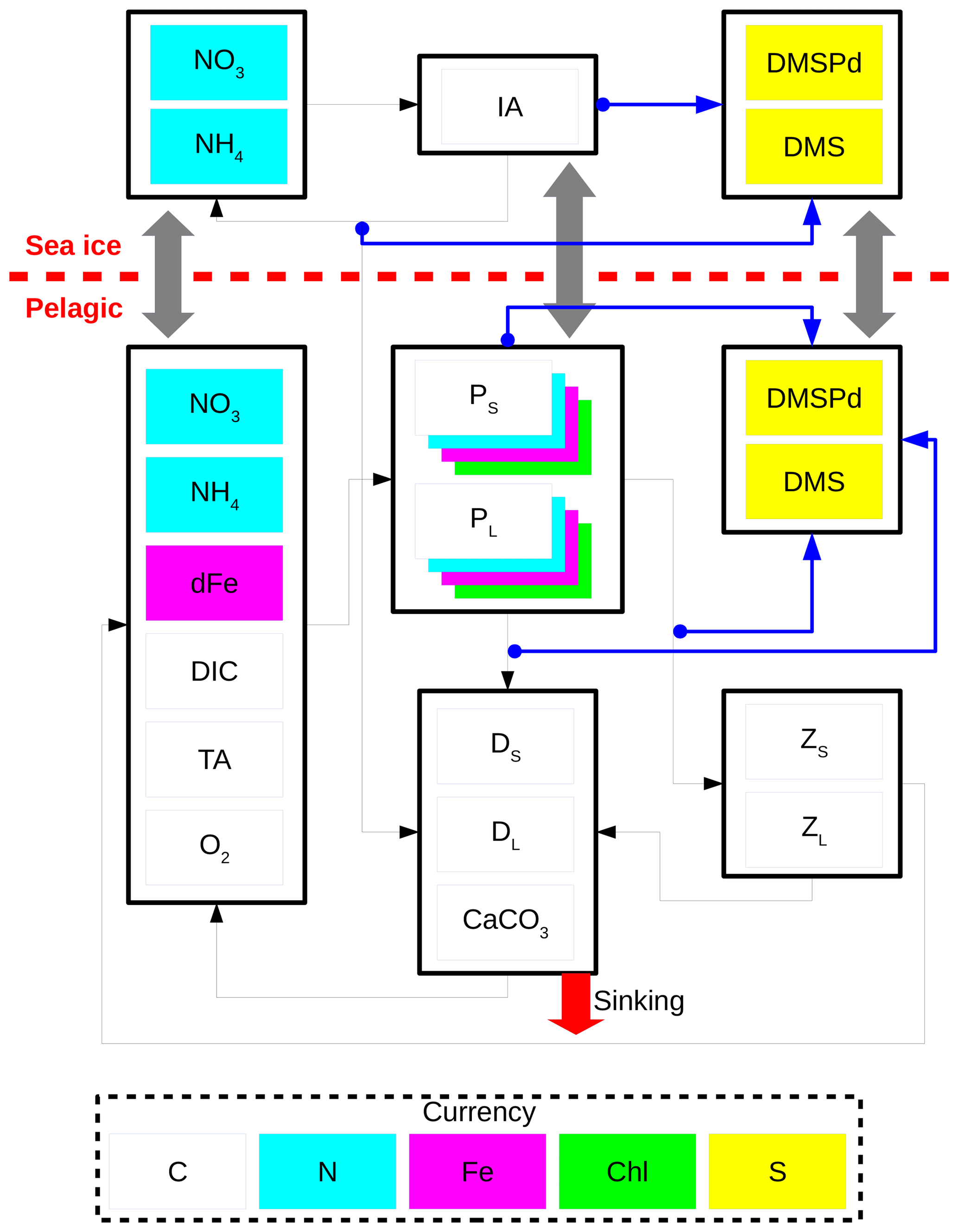
Figure 2Schematic of the CanOE pelagic ecosystem model and associated sea-ice biogeochemistry and pelagic sulfur-cycle models. Black arrows indicate fluxes of carbon (C), nitrogen (N), and iron (Fe) between compartments; blue arrows indicate sources of dissolved dimethylsulfoniopropionate (DMSPd); gray arrows indicate ice–ocean fluxes of nitrate (NO3), ammonium (NH4), ice algae (IA) and large phytoplankton (PL), DMSPd, and dimethylsulfide (DMS). Flows of dissolved oxygen (O2) are opposite to those of dissolved inorganic carbon (DIC) and are not explicitly illustrated. Detritus (DS and DL) and zooplankton (ZS and ZL) are denominated in C units but have implicit N and Fe pools according to fixed elemental ratios; phytoplankton (PS and PL) have separate state variables for each currency. O2 and total alkalinity (TA) have their own currencies, but are shown as white here for simplicity; their sources and sinks follow well established stoichiometries relative to those of DIC. Sources and sinks of TA associated with the nitrogen cycle (Wolf-Gladrow et al., 2007) are included but not shown in the figure. The state variables dFe and CaCO3 represent dissolved iron and calcium carbonate, respectively. The currencies Chl and S represent chlorophyll a and sulfur, respectively.
Also, the parameterization of sea-to-air flux of DMS was modified to account for the non-linear dependence of the flux on the open-water fraction (Loose et al., 2009):
where F is the DMS flux (µmol m−2 s−1), fow is the open-water fraction (–), kdms is the gas transfer velocity (m s−1), and DMS (nM) is the DMS concentration in the uppermost layer of the water column.
2.2.2 Correction to the fractionation of under-ice PAR
The second modification to CanOE was made to the PAR fraction of incident solar radiation. PAR is the shortwave radiation in the 400–700 nm wavelength range, which is available for photosynthesis. In CanOE, PAR is 43 % of the downwelling shortwave radiation reaching the sea surface, a well established estimate for PAR in open water (e.g., Morel, 1988). However, this assumption underestimates PAR reaching the sea surface under sea ice. The shortwave radiation penetrating through snow and ice is almost entirely PAR, as radiation outside of the 400–700 nm range is absorbed by the snow and ice (e.g., Zeebe et al., 1996). Thus, we have set the fraction of the downwelling shortwave radiation to unity (instead of 43 %) when computing the sea-surface PAR under sea ice.
2.3 Sea-ice biogeochemistry
The sub-model for sea-ice biogeochemistry is a modified version of a three-compartment (ice algae, nitrate, and ammonium) ecosystem based on Mortenson et al. (2017) and a two-compartment (DMS and DMSPd) sulfur cycle based on Hayashida et al. (2017).
Sea-ice biogeochemical processes are assumed to take place in a layer of fixed thickness at the ice base. Hence, this bottom-ice biogeochemical layer is not explicitly modelled and does not correspond to one of the two ice layers in LIM. Although algal biomass in ice core samples above this layer can be substantial (e.g., Melnikov et al., 2002; Olsen et al., 2017), resolving vertical distributions of sea-ice biogeochemistry in 3-D models is computationally impractical at present. The governing equation for any sea-ice biogeochemical state variable is
where X denotes the concentration of the state variable, denotes the horizontal velocity field of sea ice, and D denotes the horizontal eddy diffusion coefficient. The first two terms on the right-hand side of Eq. (2) represent tendencies associated with horizontal motion of sea ice (Sect. 2.3.1). The third term represents biological and chemical source minus sink (SMS). Note that while LIM2 computes the impact of mechanical redistribution (i.e., deformation due to ridging/rafting) on sea-ice physical properties, these processes are neglected in computations of the sea-ice biogeochemical state variables in the present study as the model uses a simple representation of the sea-ice biogeochemical layer as a layer of fixed thickness (3 cm) at the ice base.
2.3.1 Horizontal transport
Horizontal transport of sea-ice biogeochemical state variables is computed simultaneously and in the same way as the sea-ice physical properties of LIM2 (i.e., snow and sea-ice volume, heat content, and areal coverage). Specifically, it is done by solving the advection–diffusion equation for sea ice. Advection (by which we refer to the transport associated with the resolved motion of sea ice) is computed using the scheme of Prather (1986). Diffusion, on the other hand, represents transport by unresolved motions (random component of sea-ice motion analogous to turbulence in fluids; Thorndike, 1986; Rampal et al., 2009, 2016), and is often tuned to improve numerical stability. Diffusion is computed within the ice pack by evaluating the second-order diffusive operator using the Crank–Nicholson scheme (Crank and Nicolson, 1996), while it is set to zero at the ice edge. The horizontal diffusion coefficient (D) is set to 5 m2 s−1, as suggested by Vancoppenolle et al. (2012). The impacts of horizontal transport of sea ice on modelled biogeochemical state variables are discussed in Sect. 4.3.
2.3.2 New ice formation
The bottom 3 cm of newly formed ice is assumed to contain the same concentrations of biogeochemical state variables as those in the underlying water column. Thus, the concentration (X) of any sea-ice biogeochemical state variable is updated as follows:
where SICt−1 and SICt respectively denote the sea-ice concentrations in the previous and current time step. X∗ denotes the concentration of the sea-ice biogeochemical state variables (meltwater equivalent) after the computation of advection and diffusion but prior to the computation of biological and chemical sources and sinks. Xui denotes the concentration of the biogeochemical state variable in the uppermost layer of the water column under the ice. Equation (3) neglects the density difference between sea ice and seawater, and therefore violates mass conservation. However, this simplification has a negligible effect on ocean biogeochemistry given the relatively thin sea-ice biogeochemical layer (Hayashida et al., 2017). For ice algae only, a minimum biomass is set at 10 mmol C m−3 in order to mimic reasonable overwintering biomass. This threshold is derived based on the observed range of ice algal biomass in young sea ice (Garrison et al., 1983) and by assuming a fixed carbon-to-chlorophyll ice algal cell quota (Mortenson et al., 2017).
2.3.3 Biological and chemical sources and sinks
The biological and chemical processes represented as sources and sinks of the sea-ice biogeochemical state variables are described in detail in Mortenson et al. (2017) and Hayashida et al. (2017). For the ecosystem component, these processes include photosynthesis, mortality, and remineralization of dead organic matter. The growth rate of ice algae is dependent on ambient temperature (of underlying seawater), PAR, and nutrient concentrations (nitrate and ammonium). Note that the growth rate dependence on ice melt considered in Mortenson et al. (2017) has been neglected in the present study because (1) our preliminary results indicated that ice algal blooms were generally insensitive to it, (2) the parameterization for ice melt limitation was applied for a specific location and might not be appropriate for other locations, and (3) the parameterization lacks observational evidence.
In addition to the computation of biological and chemical sources and sinks, processes relevant to the ice–ocean fluxes are computed, including (1) turbulent molecular diffusive exchange of nutrients, (2) release of all state variables into the water column due to basal ablation, and (3) flushing of these variables by flow of water through the ice from rainfall and surface melting (including flooding due to negative freeboard). For process (1), the effects of turbulence are approximated by parameterizing the molecular sublayer as a function of friction velocity, and molecular diffusion is calculated using the observed diffusion coefficient of dissolved silica measured in seawater at 2 ∘C (Rebreanu et al., 2008).
2.4 Spatial domain
The model domain is based on the North Atlantic and Arctic (NAA) configuration developed by the ocean modelling group at the University of Alberta (http://knossos.eas.ualberta.ca/anha/model_configuration.php#naa, last access: 13 May 2019). This configuration was built on the curvilinear orthogonal coordinate system of NEMO that has been successfully applied to study the freshwater budget of the Arctic Ocean in present (Hu and Myers, 2013) and future climates (Hu and Myers, 2014), as well as to investigate pelagic ecosystem processes in the Canada Basin (Steiner et al., 2015). The NAA domain includes the Arctic Ocean, the Canadian Arctic Archipelago, the northern Bering Sea, the North Atlantic Ocean, and the Nordic Seas (Fig. 3). The horizontal resolution of the 568×400 grid varies from 10 km along the North American boundary to 14.5 km along the Eurasian boundary. Vertically, the ocean is divided into 46 layers with variable resolution, from approximately 1 m in the uppermost layer to 255 m in the bottommost layer. This vertical resolution is finer than that of the original NAA configuration in the upper layers, while it is slightly coarser in the deeper layers (approximately below the 20th level; Fig. 4). The bathymetry is based on the 1 arcmin global relief data (ETOPO1; Amante and Eakins, 2009) as described by Hu and Myers (2013). For numerical stability, each ocean grid cell is set to have at least seven vertical levels, corresponding to a depth of approximately 20 m.
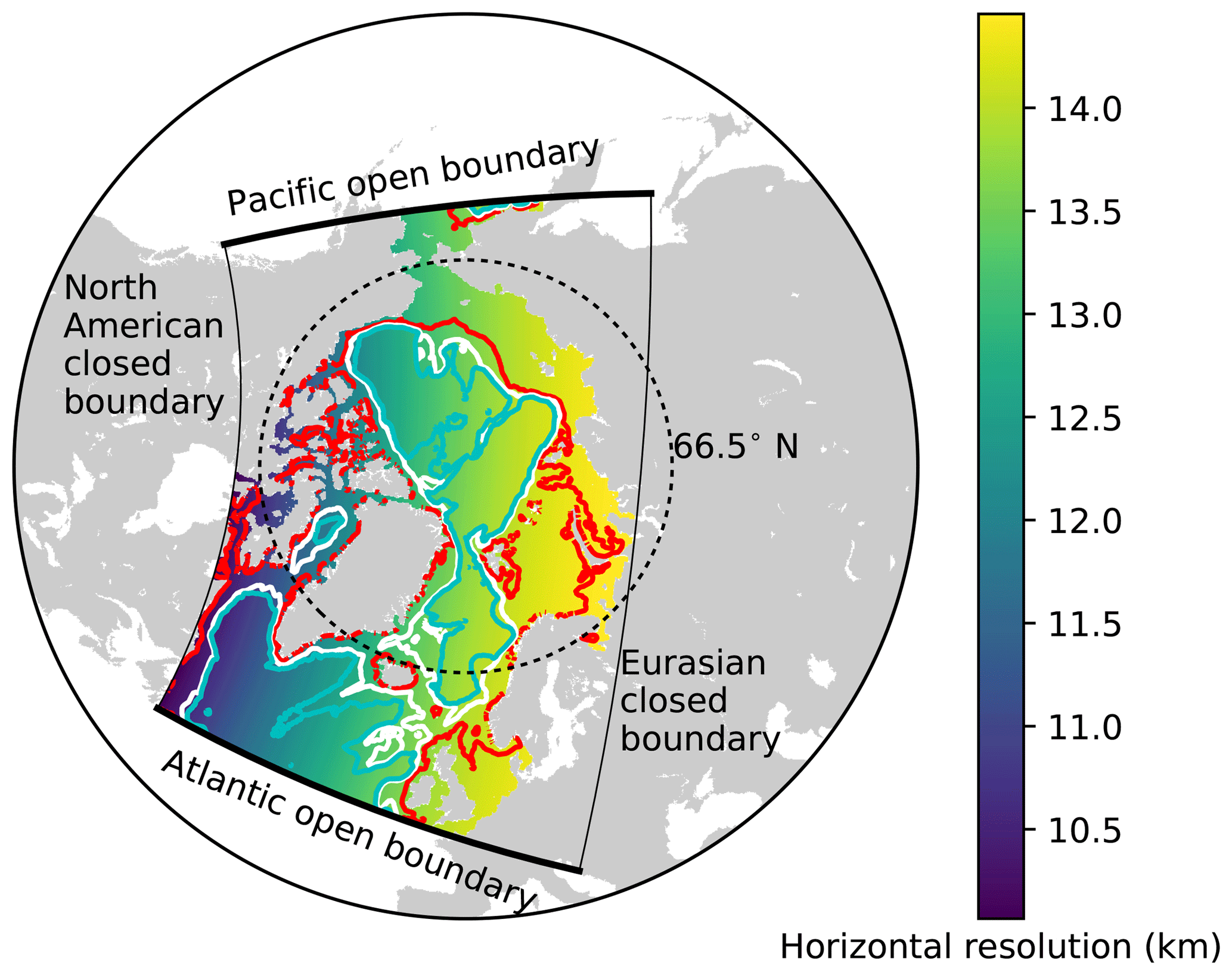
Figure 3The domain of the North Atlantic and Arctic (NAA) configuration. The colour map represents the horizontal resolution and the contour lines denote the isobaths at 100 m (red), 1000 m (white), and 2000 m (cyan). The thick (thin) solid black lines indicate the locations of Atlantic and Pacific open (North American and Eurasian closed) boundaries.
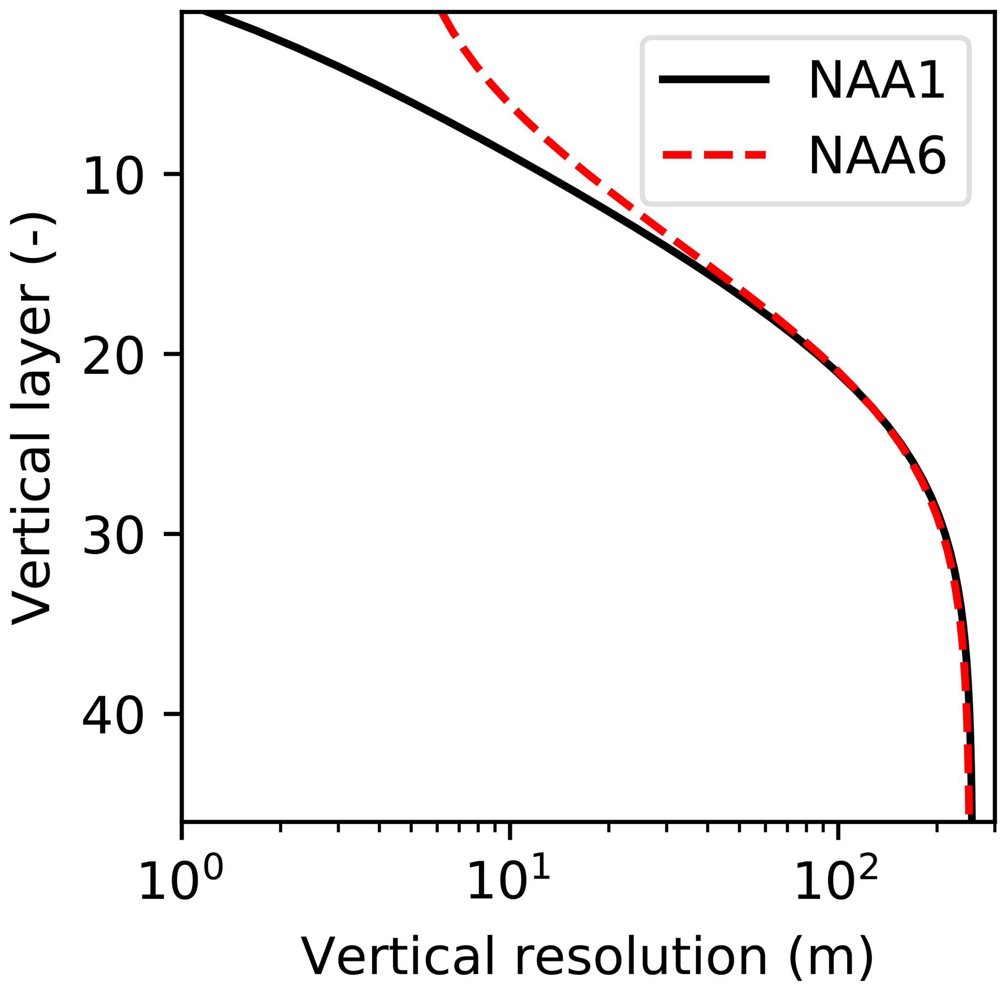
Figure 4Comparison of the vertical resolution of the ocean model between the original NAA configuration (NAA6, i.e., approximately 6 m in the uppermost layer) and the configuration adopted in the present study (NAA1, i.e., approximately 1 m in the uppermost layer). Note the log scale on the x axis.
2.5 Experiments
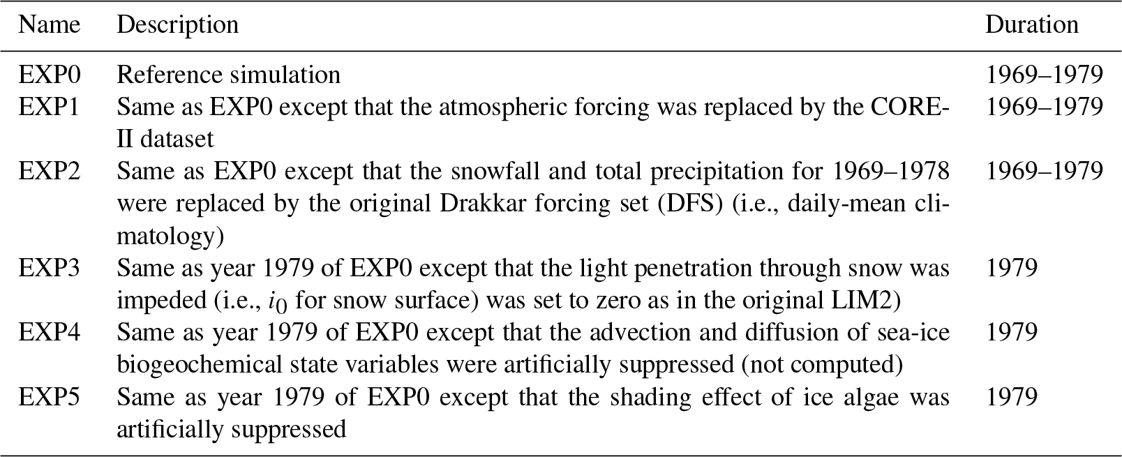
We consider six model experiments (Table 2). The first experiment is a reference simulation (EXP0), which is intended as the most realistic among all simulations considered in this study. The 11-year duration of EXP0 is considered sufficient for the spin-up of sea-ice and near-surface pelagic variables based on previous Arctic biogeochemical model studies (e.g., Dupont, 2012; Jin et al., 2012). The results during this spin-up period are presented in Appendix B. The setup of EXP0 is described below. The remaining experiments (EXP1–5) are designed to assess the sensitivity of the model simulations to changes in uncertain forcing data and parameter values.
2.5.1 Initial and lateral boundary conditions, runoff, and atmospheric forcing
The ocean was initialized from rest with temperature and salinity fields for January 1969 derived from the Ocean Reanalysis System 4 (ORAS4; Balmaseda et al., 2013). The initial snow depth, ice thickness, and ice concentration were respectively set to 0.1 m, 2.5 m, and 0.95 for grid cells with temperatures within 2 ∘C of the seawater freezing point. Elsewhere, these values were set to zero. The initial concentrations of nitrate, dissolved inorganic carbon, and total alkalinity were taken from the annual-mean fields of the GLobal Ocean Data Analysis Project version 2 (GLODAP2; Lauvset et al., 2016). The initial concentrations of dissolved oxygen were set to the annual-mean fields from the World Ocean Atlas 2013 Version 2 (WOA13; Garcia et al., 2014). The initial concentration of dissolved iron was set to 0.6 nM in the entire domain (Aumont et al., 2015). Because the model simulation starts at a time of low biological production (i.e., 1 January), the remaining biogeochemical state variables in the ocean were initialized uniformly in space to very low values (e.g., 0.01 mmol C m−3 for the carbon contents of phytoplankton, zooplankton, and detritus). The initial concentrations of sea-ice biogeochemical state variables were set to the same values as their respective variables in the uppermost layer of the ocean.
Open boundary conditions were applied by a radiation-relaxation algorithm (Madec, 2008) along the Atlantic and Pacific boundaries of the model domain, while the other two boundaries (along North America and Eurasia) were assumed to be closed (Fig. 3). The boundary temperature, salinity, and zonal and meridional current fields were interpolated from the interannual monthly-mean fields of ORAS4. The open boundary conditions for ocean biogeochemical state variables were the same as their initial conditions. The relaxation timescales were set to 1 d for inflow and 15 d for outflow. These values are identical to those used in Dupont et al. (2015), but differ from the original NAA configuration (Hu and Myers, 2013). Our preliminary experiments suggested that these changes were needed to prevent salinity drift. Because the feature to prescribe the open boundary conditions for the sea-ice prognostic variables was not available in NEMO version 3.4, these were set to zero for the sea-ice prognostic variables of LIM2 as well as the sea-ice biogeochemical state variables; this feature is available in the subsequent version of NEMO (version 3.6).
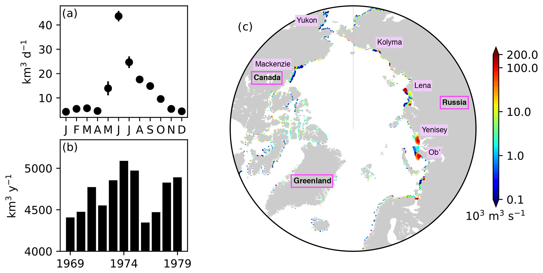
Figure 5River runoff of freshwater prescribed in the model. (a) Annual cycle of daily discharge and (b) interannual variability in annual discharge integrated over the region north of 60∘ N. (c) Spatial distribution of annual discharge rate averaged over the period 1969–1979. In panel (a), the error bars indicate the standard deviations over the period 1969–1979. In panel (c), note the log scale on the colour bar, and names of major rivers and countries or regions are labelled.
River discharge of freshwater was derived from the interannual monthly-mean product of Dai and Trenberth (2002). Figure 5 shows the seasonal and interannual variability (panels a and b) and spatial distribution (c) of the total discharge over the pan-Arctic. The river discharge of biogeochemical state variables was neglected due to the lack of adequate data. Additional external supplies of nutrients (dust deposition and sediment mobilization) were neglected due to the lack of reliable data. Partial pressure of carbon dioxide in the atmosphere was derived from the monthly-mean Mauna Loa CO2 data (https://www.esrl.noaa.gov/gmd/ccgg/trends/data.html, last access: 19 April 2017).
The surface atmospheric conditions used to drive the sea-ice and ocean model simulations were derived from the Drakkar forcing set 5.2 (DFS; Dussin et al., 2016). The DFS dataset has high resolutions in space (0.7∘) and time (3-hourly for zonal and meridional wind speed at 10 m height as well as air temperature and specific humidity at 2 m height, and daily for incoming shortwave and longwave radiation, total precipitation, and snowfall). It is based on a combination of ERA-40 and ERA-Interim reanalysis products (Uppala et al., 2005; Dee et al., 2011). The original DFS dataset (https://www.drakkar-ocean.eu/forcing-the-ocean, last access: 13 May 2019) has missing data flags which cause a simulation crash in some years. As a substitute, we used a version provided by Clark Pennelly at the University of Alberta (personal communication) which addressed the missing data flag errors without any modifications to the atmospheric data (the only changes were indexing and ordering of latitudinal coordinates and remaining variables). In the original DFS dataset, the daily total precipitation (rain and snow) and snowfall fields prior to 1979 were set to their respective 1979–2012 climatological daily averages due to the lack of adequate observations to construct the dataset for those years individually (Dussin et al., 2016). However, in EXP0, we prescribed the total precipitation and snowfall for 1979 repeatedly for the simulation over the period 1969–1978, while keeping the remaining atmospheric variables the same as the original DFS dataset. This modification was necessary to simulate adequate snow depths (discussed further in Sect. 4.1).
2.5.2 Additional settings
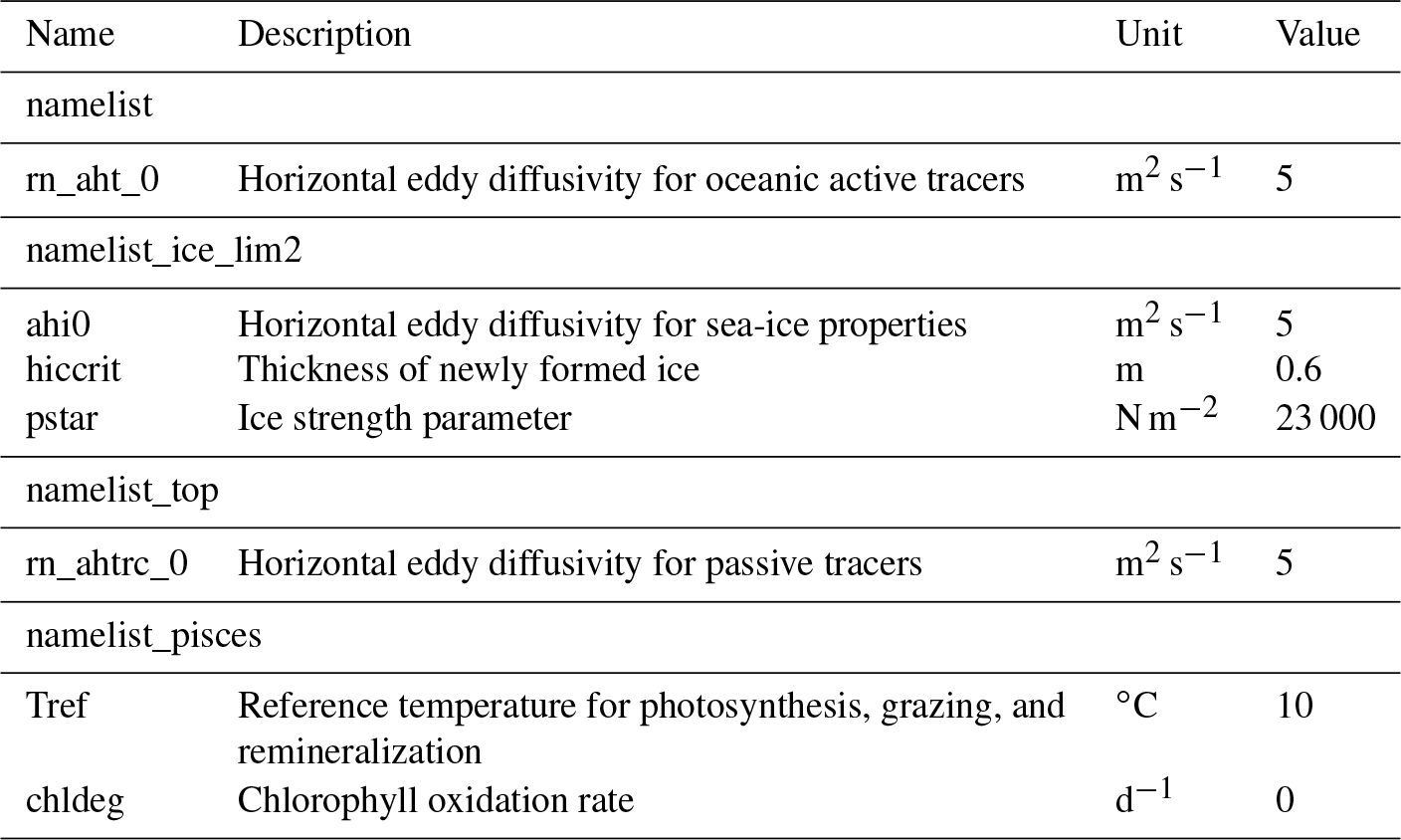
The time step of the model integration was 20 min. Unlike Hu and Myers (2013), no additional treatments for modelled temperature, salinity, or wind-stress fields near the open boundaries were necessary since no obvious drift was apparent in the simulated fields. Table 3 displays some of the model parameters that were modified from their default values in NEMO v3.4. For a complete list of the parameters, readers are referred to the source-code repository (https://doi.org/10.5281/zenodo.1435254). The coefficients for horizontal eddy diffusion for oceanic and sea-ice tracers (rn_aht_0, ahi0, and rn_ahtrc_0) were reduced to keep diffusion relatively small compared to resolved dynamical processes, as recommended by Vancoppenolle et al. (2012). The other two parameters (hiccrit and pstar) were adjusted to improve the fit with the PIOMAS data product (Sect. 2.6) in terms of sea-ice volume and extent for 1979 (Sect. 3.1.1). While parameter hiccrit is very large considering that it is the initial thickness of newly formed ice, it is also known as a tuning parameter for sea-ice extent in LIM (Wang et al., 2010; Roy et al., 2015). Hence, we chose this value while trying to keep it low as much as possible. Lastly, two parameters of CanOE (Tref and chldeg) were adjusted to simulate reasonable annual primary production in the Arctic Ocean (Sect. 3.2). Note that chldeg is a parameter for photo-oxidation designed specifically for the global configuration of CanOE to tune the global chlorophyll distribution, and therefore we set this to zero in our Arctic configuration.
Table 3List of selected model parameters in the NEMO namelists.
2.5.3 Output
The output of the model experiments was saved as annual means for the first 10 years (1969–1978) and 5-day means for the final year (1979). Ice (snow) volume was defined as the sum of the product of grid-cell-mean ice thickness (snow depth) and the grid-cell area. Ice extent was defined as the areal sum of all grid cells with an ice concentration of at least 0.15. Primary productivity of ice algae and phytoplankton was quantified in terms of depth-integrated (bottom 3 cm of sea ice and upper 90 m of water column, respectively) net primary productivity (NPP). Ice algal NPP is assumed to equal the growth term in the model equation (Mortenson et al., 2017), as the specific growth rate associated with that term is derived from Eppley (1972). This rate is a measure of particulate production, which is considered to provide values closer to NPP than gross primary productivity (GPP) (e.g., Sakshaug et al., 1997; Hashimoto et al., 2005). Thus, the loss due to respiration is implicitly included in the growth term in the model equation for ice algae. On the other hand, CanOE has an explicit representation of respirational loss, and so phytoplankton NPP is defined as the growth minus the respiratory cost of biosynthesis (Christian et al., 2019; see Appendix A3 of Hayashida, 2018a). For the analysis of NPP and PAR only, any grid cell whose ice concentration is 0.15 or greater was considered “under-ice” following Zhang et al. (2010). To investigate the interannual variability in pan-Arctic primary productivity, the ice algal NPP, phytoplankton NPP, and under-ice NPP were integrated annually and horizontally to derive respective pan-Arctic annual quantities. The term pan-Arctic is defined here as the region north of the Arctic Circle (66.5∘ N). The pan-Arctic mean refers to an area-weighted average over the region north of the Arctic Circle. This areal restriction allows for a consistent comparison to some previous studies (e.g., Legendre et al., 1992; Jin et al., 2012).
2.6 PIOMAS data product
The modelled sea-ice properties were evaluated against the output of the Pan-Arctic Ice Ocean Modeling and Assimilation System (PIOMAS), which is a regional coupled sea-ice–ocean circulation model that assimilates some observational data (Zhang and Rothrock, 2003; Schweiger et al., 2011). The monthly-mean ice thickness and ice concentration gridded data products of PIOMAS were interpolated onto the NAA grid in order to perform a grid-to-grid comparison across the same domain. Although the PIOMAS data product is considered here as the best presently available, note that it has its own biases that could result in mismatches with our model results.
3.1 Comparison of sea-ice physical properties with PIOMAS in 1979
3.1.1 Seasonal variability
To assess the model performance in simulating sea ice, the seasonal variability of modelled ice volume and extent in EXP0 are compared to PIOMAS (Fig. 6a and b) for 1979 (after a decadal spin-up). In both EXP0 and PIOMAS, the annual maximum in ice volume (extent) takes place in April (March), while both the ice volume and extent are at their annual minima in September. The ice volume is consistently higher in EXP0 than PIOMAS. The difference in the annual-mean ice volume over the NAA domain is 3.9 km3 (17 %). In contrast, the ice extent comparison is much better with the difference of 0.1×10⁶ km2 (1 %) in the annual means.
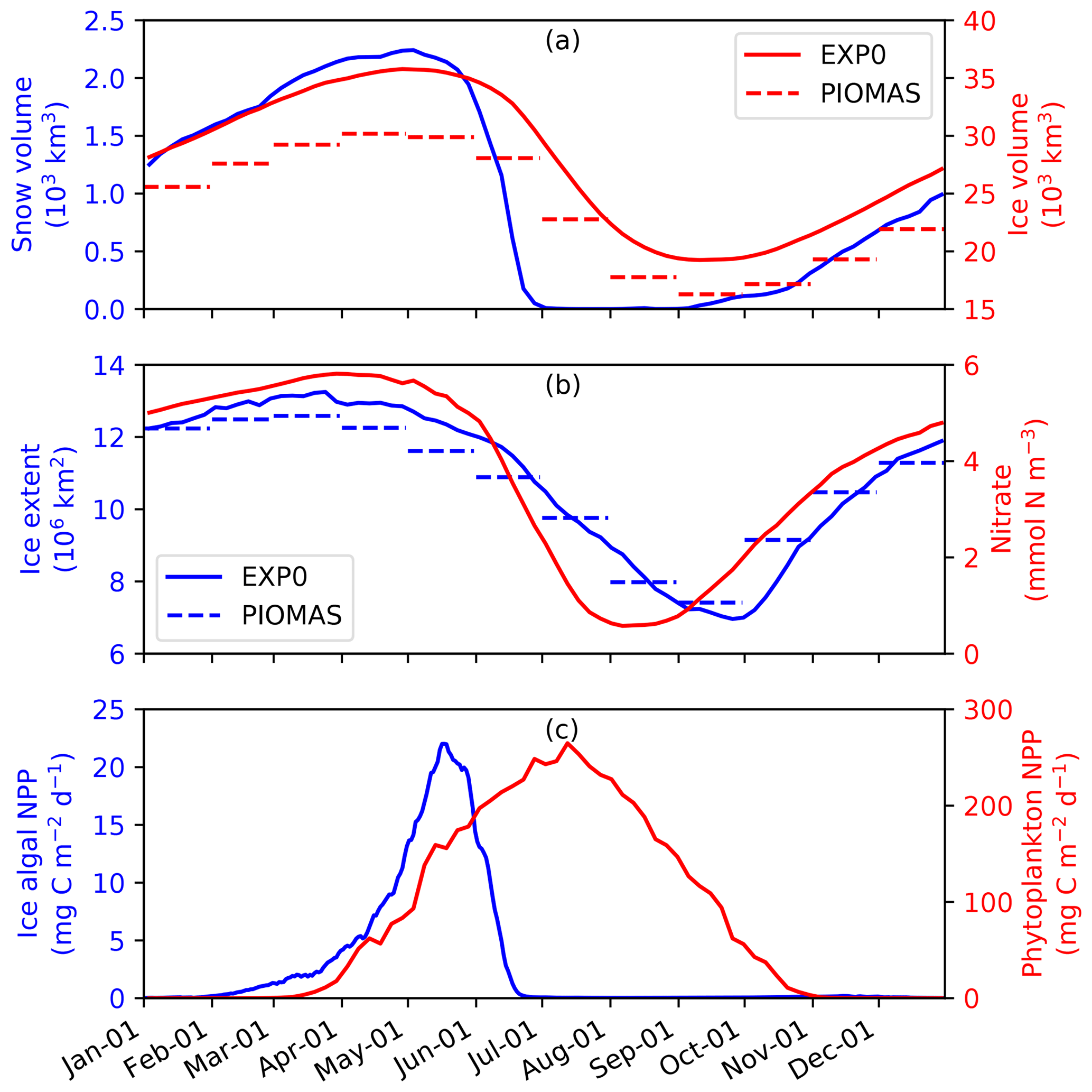
Figure 6Time series of 5 d mean modelled (a) snow and ice volumes, (b) ice extent, and pan-Arctic-mean surface seawater nitrate concentration, and (c) pan-Arctic ice algal and phytoplankton NPP during 1979 in EXP0. The dashed lines in panels (a) and (b) represent the monthly-mean PIOMAS ice volume and extent, respectively.
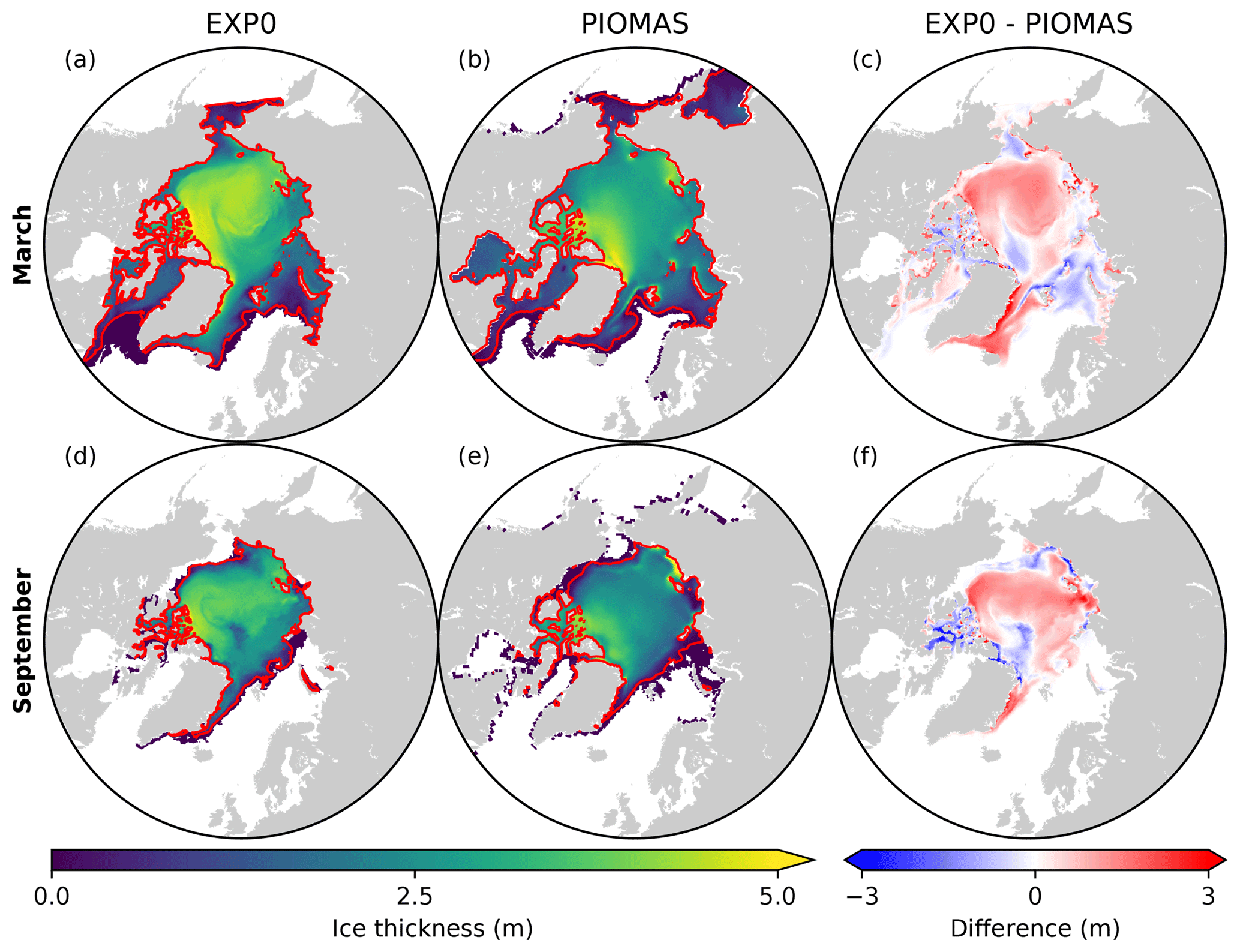
Figure 7Spatial distributions of monthly-mean ice thickness in EXP0 (a, d) and the PIOMAS product interpolated onto the NAA grid (b, e) and their difference (c, f) for March and September in 1979. The red lines represent the ice edge, defined here as the 0.15 contour of ice concentration.
3.1.2 Spatial variability
Figure 7 shows the spatial variability in modelled March- and September-mean ice thickness fields in EXP0 and PIOMAS. The extent of modelled Arctic sea ice can be inferred from the location of the ice edge, defined here as the 0.15 contour of ice concentration (Fig. 7a, b, d, e). Overall, the locations of the ice edge within our model domain are similar between EXP0 and PIOMAS for both March and September. Beyond the model domain, the ice coverage in March extends to Hudson Bay and the Sea of Okhotsk in PIOMAS (Fig. 7b). The March-mean ice thickness distribution in EXP0 includes a band of >5 m thick ice along the coast of the Canadian Arctic Archipelago extending east to Greenland, and a region of relatively thick ice (∼4 m) in the Arctic Basin north of the East Siberian Sea (Fig. 7a). The band is also present in PIOMAS, although it is restricted to the north of Greenland (Fig. 7b). The thick-ice region in the Arctic Basin north of the East Siberian Sea, on the other hand, is absent in PIOMAS. Besides these particular regions, EXP0 generally simulates thicker ice than PIOMAS in the Greenland Sea and various shelf regions (Fig. 7c). On the other hand, EXP0 simulates thinner ice than PIOMAS on the Canadian Polar Shelf and in the Chukchi Sea, the Barents Sea, the Kara Sea, and an area near the North Pole (Fig. 7c). Overall, the mean absolute difference in the ice thickness distribution over the NAA domain is 0.43 m (30 %). Note that the difference is still calculated even if the ice is absent by considering a thickness of 0 m. Also, note that even though PIOMAS assimilates data, it is still a model product, and therefore the difference is not a definite measure of accuracy.
In September, the most notable features in the ice thickness distribution are the presence of thinner (<2 m) ice in an area near the North Pole in EXP0 (Fig. 7d) and thicker (>5 m) ice along the coast of Siberia in PIOMAS (Fig. 7e). While the latter feature is not discussed in any of the literature on PIOMAS, it seems unrealistic considering that it is thicker in September than in March and it is thicker than the multi-year ice present along the band north of the Canadian Arctic Archipelago and Greenland. Both of these features constitute negative ice thickness anomalies in the model relative to PIOMAS (Fig. 7f). The difference is also negative and large (∼3 m) on the Canadian Polar Shelf; this could be due to the fact that the horizontal resolution of PIOMAS (∼22 km; Zhang et al., 2010) is too coarse to resolve the circulation through these relatively narrow channels, resulting in the simulation of first-year ice that is too thick in this region at this particular time of the year. The ice thickness is greater in EXP0 than in PIOMAS in the Arctic Basin, part of the East Siberian Sea, and the Laptev Sea as well as along the eastern coast of Greenland. The mean absolute difference is 0.31 m (38 %), similar to the March comparison.
3.2 Primary productivity of ice algae and phytoplankton
3.2.1 Seasonal variability
Figure 6 shows the seasonal variability in modelled pan-Arctic-mean ice algal NPP and phytoplankton NPP during 1979 (panel c) along with relevant environmental factors (panels a and b). Ice algal NPP starts increasing in early February, peaks in mid-May, sharply declines in late May to early June, and is near zero by late June. The start of the decline of the ice algal NPP coincides with the decline of the ice volume (Fig. 6a) demonstrating that the decline is driven by the release of ice algae as a result of ice melt. The seasonal progression of the ice algal production is similar to Jin et al. (2012). The phytoplankton NPP starts increasing in early March, peaks in early July, and decreases to near zero by the end of October (Fig. 6d). At the peak in phytoplankton NPP, the pan-Arctic-mean surface seawater nitrate concentration is below 1 mmol N m−3 and remains so until the end of August (Fig. 6b).
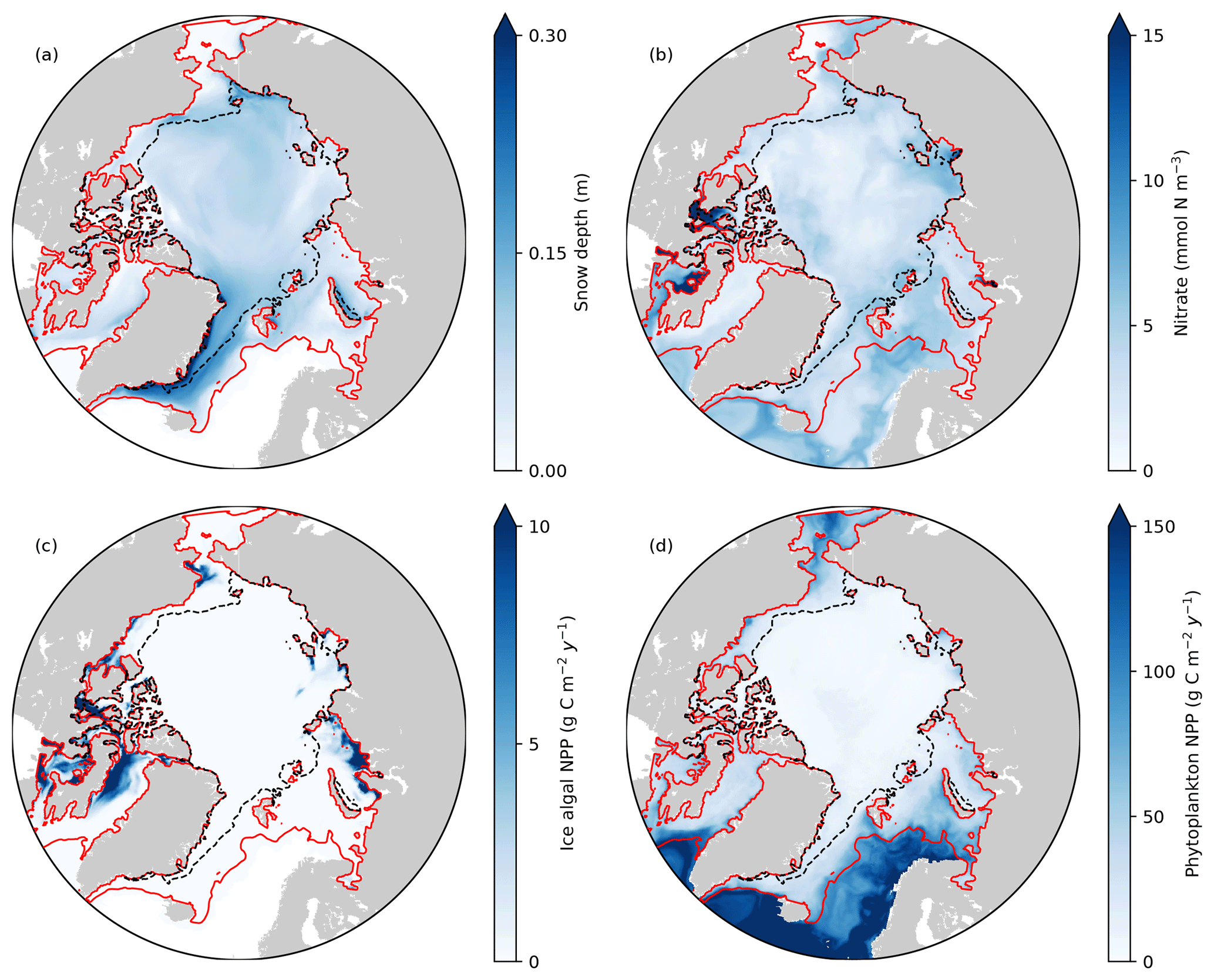
Figure 8Spatial distribution of annual-mean (a) snow depth and (b) surface seawater nitrate concentration, and (c) depth-integrated (bottom 3 cm) ice algal annual NPP and (d) depth-integrated (upper 90 m) phytoplankton annual NPP in 1979 in EXP0. The red and black dashed lines represent the 0.15 contour of monthly-mean ice concentration in March and September, respectively.
3.2.2 Spatial variability
Figure 8 shows the spatial distribution of annual-mean snow depth, surface seawater nitrate concentration, ice algal NPP, and phytoplankton NPP for 1979. The largest values of ice algal annual NPP (>10 g C m−2 yr−1) are present on the Canadian Polar Shelf and in the coastal regions of Baffin Bay, the Chukchi Sea, the East Siberian Sea, and the Kara Sea (Fig. 8c). All of these regions have relatively thin snow (less than 0.1 m; Fig. 8a), demonstrating the control of light on ice algal growth. In contrast, the nutrient control on ice algal production is less pronounced; although high ice algal NPP usually coincides with high surface seawater nitrate, it is also present in a few areas where the nitrate levels are relatively low (Baffin Bay and Chukchi Sea; Fig. 8b). Overall, ice algal production is mostly confined to shelf regions (excluding the Barents Sea), consistent with previous model studies (Deal et al., 2011; Dupont, 2012; Jin et al., 2012, 2018).
There are a few noteworthy similarities and differences in the spatial variability in modelled ice algal annual production between the present study and previous model studies. All studies show a moderate-to-high level of ice algal production in Baffin Bay. In contrast, disagreement in the ice algal production is found along the eastern coast of Greenland and in the Bering Sea; the values along the eastern coast of Greenland are moderate (5–10 g C m−2 yr−1) in Deal et al. (2011) and Jin et al. (2012), while they are low (less than 5 g C m−2 yr−1) in Dupont (2012), Jin et al. (2018), and the present study. Similarly, although the Bering Sea is identified as a region of high ice algal production by Deal et al. (2011), Jin et al. (2012), and Jin et al. (2018), Dupont (2012) and the present study simulate low ice algal production in this region. A possible explanation for the lower ice algal production in this region in the latter studies is an insufficient nutrient supply from the Pacific boundary as discussed in Dupont (2012). Lastly, the recent study by Jin et al. (2018) finds the Sea of Okhotsk to be a region of elevated ice algal annual production, which we are unable to assess in the present study due to the limited model domain. We also note the difference in the temporal coverage of simulations among these studies, which can explain some of the differences in these results.
The modelled phytoplankton annual NPP is high (>100 g C m−2 yr−1) in the Atlantic and the Pacific sectors with little-to-no ice cover, moderate (50–100 g C m−2 yr−1) in the shelf seas along the North American and the Eurasian continents, and low (<50 g C m−2 yr−1) in the interior of the Arctic Ocean (Fig. 8d). These findings are in quantitative agreement with the results of five different models and satellite-based estimates (Fig. 1 of Popova et al., 2012).
3.2.3 Interannual variability
The modelled pan-Arctic ice algal annual NPP in EXP0 ranges from 10.5 to 18.2 Tg C yr−1 for the period 1970–1979, excluding the initial spin-up year. While this value is on the lower end of the range of observation-based NPP estimates (9–73 Tg C yr−1; Legendre et al., 1992), it is close to the decadal mean of the annual NPP (10.1 Tg C yr−1 for 1998–2007) simulated by Jin et al. (2012). The pan-Arctic estimates by Legendre et al. (1992) are quite speculative as they are based on the integration of a single ice algal production value over a specified ice area (discussed in detail in Deal et al., 2011). The close agreement between the two model-based estimates suggests that the lower end of the observation-based estimates is more plausible than their upper end. Although the upper end accounts for contribution from mat and strand communities that are not represented in our model (representing them would require additional state variable(s) and/or new formulation with more parameters), their contribution to the pan-Arctic production should be small as their spatial distribution is generally localized (e.g., Assmy et al., 2013). Direct comparisons with the results of Deal et al. (2011) and Dupont (2012) are not possible because the reported values in those studies include contributions from below the Arctic Circle. The modelled pan-Arctic phytoplankton annual NPP in EXP0 ranges from 378 to 465 Tg C yr−1, which is in line with the observation-based estimate (>329 Tg C yr−1; “Total High Arctic”) of Sakshaug (2004) and the satellite-based estimate (419 Tg C yr−1 for 1998–2006) of Pabi et al. (2008), but below the model-based estimate (627 Tg C yr−1 for 1998–2006) of Jin et al. (2012).
3.3 Vertical distribution of salinity, nitrate, chlorophyll a, and DMS in the upper water column
The seasonal variability in pan-Arctic-mean seawater salinity, nitrate, chlorophyll a, and DMS in the upper 15 m of the water column is shown in Fig. 9. During the summer, a prominent freshening of the uppermost layer occurs as a result of ice melt (Fig. 9a). This freshening results in the formation of a thin layer of low-salinity water known as a meltwater lens, which strengthens stratification and reduces mixing with the underlying water column. The formation of the lens coincides with the bloom of modelled phytoplankton, resulting in the depletion of nitrate first in the uppermost model layer and then in the underlying layers (Fig. 9b). Nutrient depletion in the near-surface waters then results in the formation of subsurface chlorophyll a and DMS maxima during the latter half of July (Fig. 9c and d). Note that the meltwater lens and the subsurface maxima are respectively thicker and shallower than those observed by field measurements (e.g., Brown et al., 2015) because of averaging over the pan-Arctic domain. The purpose of this spatial averaging is to quantify the impacts at a larger scale rather than assessing localized effects. Note that the model does simulate reasonable subsurface chlorophyll a maxima compared to observations (Appendix C). On the other hand, the modelled salinity distribution shows a fresh bias compared to the Polar Hydrographic Climatology version 3.0 (PHC3.0; Steele et al., 2001) throughout the year in the upper water column and most substantially (>2 psu) in the surface layer (Fig. S1 in the Supplement).
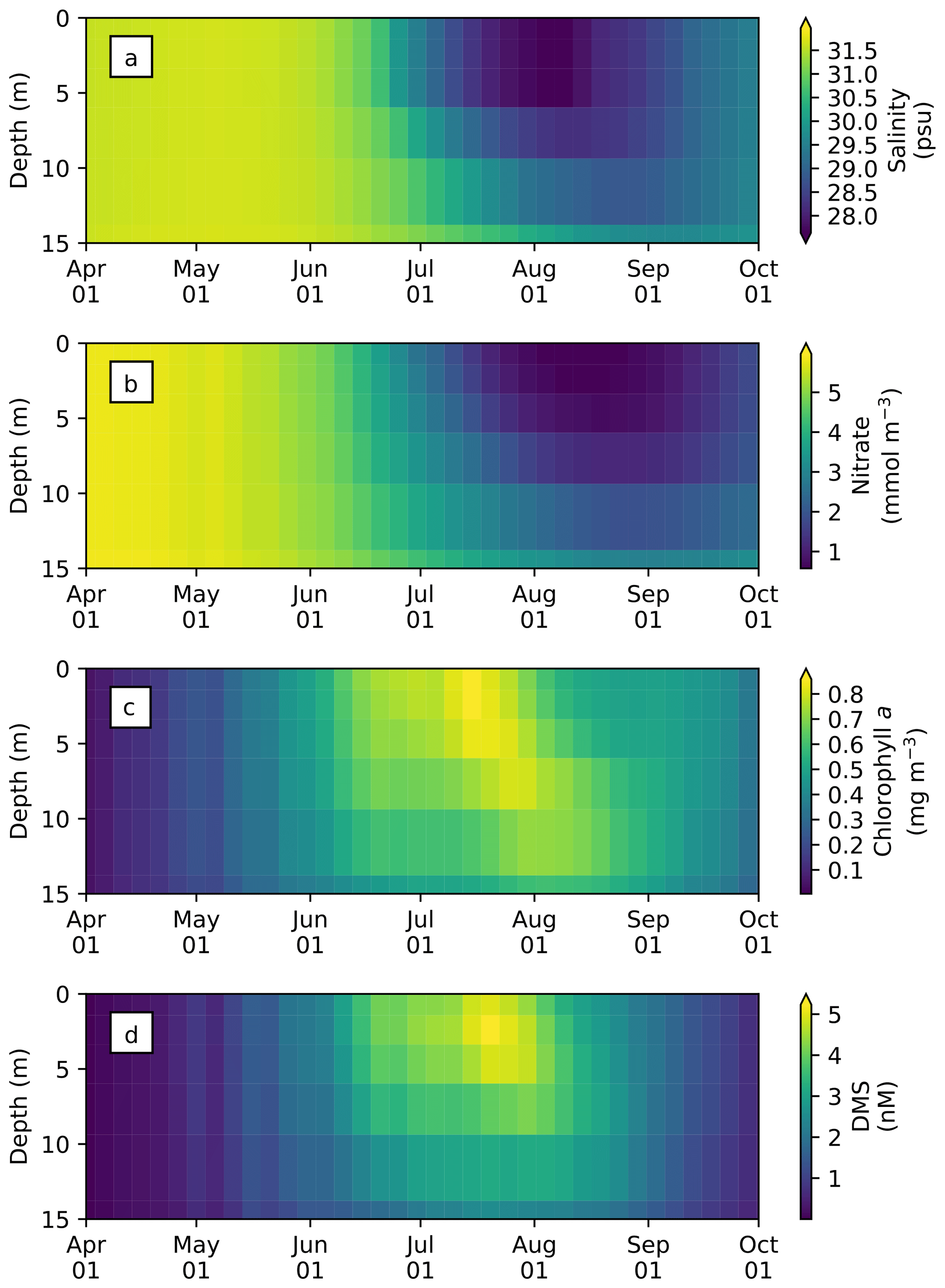
Figure 9Time series of 5 d mean and pan-Arctic-mean seawater (a) salinity, and concentrations of (b) nitrate, (c) chlorophyll a, and (d) DMS in the upper 15 m of the water column during April–September in 1979 of EXP0.
These ice-associated physical and biogeochemical processes take place within a relatively shallow upper-water column (∼10 m), and would have been impossible to simulate with a model of coarse vertical resolution. It is for this reason that the near-surface vertical resolution of the NAA configuration considered in the present study is finer than that of the original configuration (6 m in the uppermost layer; Hu and Myers, 2013). Although modelling these small-scale processes probably has a negligible effect on bulk quantities such as depth-integrated NPP, it can have an impact on processes at the air–sea or ice–sea interface (e.g., gas fluxes). To illustrate this point, the time series of modelled pan-Arctic-mean seawater DMS concentration in the uppermost layer of the water column (about 1 m) is compared with the concentration averaged over the top four layers (about 12 m) as a proxy for values simulated by a coarse-vertical-resolution model (Fig. 10).
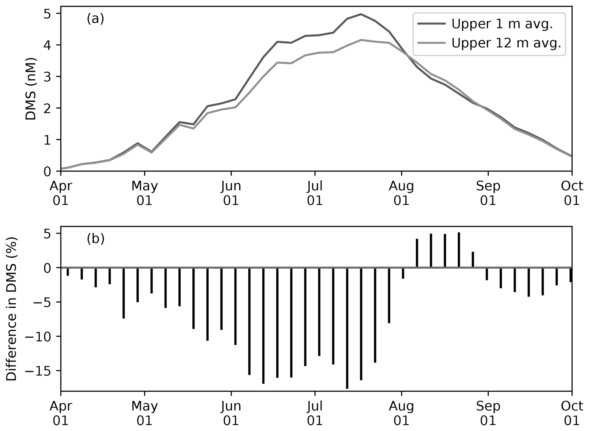
Figure 10(a) Time series of 5 d mean and pan-Arctic-mean seawater DMS concentration (a) in the uppermost layer (∼1 m; black) and averaged over the upper four layers (∼12 m; gray) during April–September in 1979 of EXP0. (b) The percentage difference between the two time series (the 12 m average minus the 1 m average, divided by the 1 m average).
Modelled DMS concentration is higher in the uppermost layer than the 12 m average throughout most of April–September, while it is slightly lower in August (Fig. 10a). The concentration difference is highest (up to about 20 %) in June–July (Fig. 10b). Overall, the annual-mean DMS concentration averaged over the upper 12 m of the water column is 9 % lower than in the upper 1 m. Here, the averaging over a thicker layer results in dilution of the DMS concentration in the uppermost layer represented in the model. Considering that this difference is present primarily during the ice melt period, and therefore that the sea-surface DMS is released into the atmosphere, the modelled sea-to-air DMS flux would be underestimated by a similar amount in the absence of fine vertical resolution in the upper water column.
4.1 Snowfall forcing frequency (EXP1 and 2)
Two sensitivity experiments (EXP1 and EXP2) are performed with the identical setup as EXP0 except for a change to the atmospheric forcing. In EXP1, all the forcing fields are replaced by the CORE-II dataset as in the original NAA configuration (Hu and Myers, 2013). Note that the temporal resolution of the snowfall and total precipitation fields in the CORE-II dataset is monthly. In EXP2, the snowfall and total precipitation fields over the period 1969–1978 are replaced by their respective 1979–2012 daily climatological values as in the original DFS dataset (Dussin et al., 2016). Comparing between EXP0 and EXP1 allows us to assess the impacts of atmospheric forcing (DFS vs. CORE-II), while comparing between EXP1 and EXP2 allows us to assess the impacts of snowfall dataset (daily vs. daily climatology) on modelled snow depth.

Figure 11Model sensitivity to snowfall forcing frequency. Time series of pan-Arctic-mean (a) prescribed snowfall rate of the CORE-II (blue) and DFS (black/red) datasets and (b) modelled annual-mean snow depth in EXP0 (black), EXP1 (blue), and EXP2 (red). Spatial maps of modelled annual-mean snow depth for the period 1970–1978 in (c) EXP0, (d) EXP1, and (e) EXP2. The units for the snowfall rate are converted from kilogram per square metre per second (kg m−2 s−1) to millimetre per day (mm d−1) using a constant snow density of 330 kg m−3, which is the value assumed in LIM2. In EXP0, the snowfall rate for 1979 is repeated annually throughout 1969–1979.
A comparison of the pan-Arctic-mean snowfall rates between the CORE-II and DFS datasets illustrates the differences between them (Fig. 11a). The monthly CORE-II dataset varies from approximately 1 to 2.4 mm d−1 (meltwater equivalent), while the range of the DFS dataset is 3 times as large (from near 0 to about 4.4 mm d−1 for the year 1979) most likely due to the difference in the temporal resolution of the datasets. The lack of high-frequency variability in the DFS daily climatology is evident from the comparison of the DFS dataset between 1969–1978 and 1979. The daily climatology ranges approximately from 0.2 to 2.2 mm d−1, less than half of the range for the individual daily averages for 1979. The annual-mean CORE-II snowfall rate is higher than that of the DFS dataset in all of these years. The annual mean of the DFS daily climatology is slightly greater than that of the individual daily averages for 1979.
Figure 11b shows a comparison of the modelled pan-Arctic annual-mean snow depth time series among EXP0, EXP1, and EXP2. The snow depth is substantially lower in EXP1 and EXP2 than in EXP0 throughout the period 1969–1979, except for 1969 (in which year the snow depth is affected by its initial value). In EXP2, the extremely low snow depth somewhat recovers in 1979. Figure 11c–e shows a spatial comparison of the modelled annual-mean snow depth over the period 1970–1978 (excluding the first and last year of simulation). There is a clear difference in the distribution between EXP0 and the other two experiments; the ice pack is generally covered by a moderate amount of snow (∼0.1 m) in EXP0, while in EXP1 and EXP2, most regions are nearly snow-free. These results of the latter two experiments are inconsistent with the available snow depth climatology indicating the presence of considerably thicker (>0.2 m) annual-mean snow cover over the Arctic Basin (Warren et al., 1999). As a result of these biases, the modified DFS dataset is used as the reference simulation, rather than the CORE-II dataset or the original DFS dataset.
The results of these sensitivity experiments demonstrate the need for high temporal resolution forcing for snowfall datasets in order to realistically simulate snow depth. The lack of snow accumulation in EXP1 and EXP2 is likely due to the mismatch between the timing of snowfall and the state of ice surface (freezing or melting). The latter is also determined by the forcing dataset (air temperature), which has relatively high temporal resolution (3-hourly for DFS and 6-hourly for CORE-II). Ideally, the temporal resolutions of snowfall and air temperature should be identical for consistency, such that snowfall occurs when air temperature is at or below freezing. Such an effort has been made recently (Tsujino et al., 2018), which should resolve the issue illustrated in our sensitivity experiments. Although the usage of a high-frequency atmospheric forcing dataset is desirable, our further sensitivity experiments indicate that the issue can be resolved by tuning another model parameter, which is presented for readers' interest in Appendix D.
4.2 Light penetration through snow column (EXP3)
Figure 12 compares the modelled sea-ice physical and biogeochemical properties in 1979 in EXP0 with those of EXP3, in which i0 for snow surface is set to the default LIM2 value of zero. The results for modelled snow and ice volume are almost identical between the two experiments (Fig. 12a), indicating a low sensitivity of these physical quantities to the change in i0 for the snow surface. On the other hand, an appreciable difference in the modelled bottom-ice PAR prior to the melt season in June results in a large difference in the modelled ice algal NPP (Fig. 12b). Ice algal NPP in EXP3 is restricted to snow-free regions, so an increase in the ice algal NPP due to the change in i0 for snow surface reflects production in snow-covered regions (Fig. 12c). The pan-Arctic ice algal annual NPP of EXP3 is 3.5 Tg C yr−1, only about a quarter of the value obtained in EXP0. This value is much lower than those obtained in previous studies (see Sect. 3.2.3). This result emphasizes the importance of correct representation of the light penetration through snow, and shows that the original LIM2 provides inadequate light for ice algal growth, resulting in insufficient ice algal NPP. Note that the default value of i0 for the snow surface is also set to zero in LIM3 (Vancoppenolle et al., 2012).
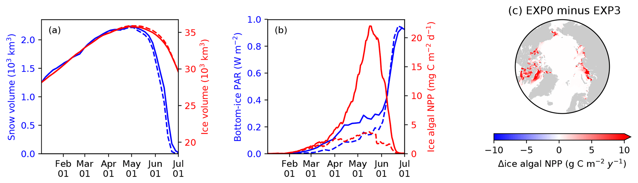
Figure 12Model sensitivity to light penetration through snow. Time series comparison of modelled 5 d mean (a) snow volume (blue) and ice volume (red) and (b) bottom-ice PAR (blue) and ice algal NPP (red) in 1979 between EXP0 (solid) and EXP3 (dashed). (c) Spatial distribution of the difference in the ice algal annual NPP between EXP0 and EXP3.
Previous 3-D sea-ice biogeochemical models differ in their choices of values for i0 for the snow surface (Table 1). The studies of Dupont (2012) and Jin et al. (2012) set this value to zero, yet their values for simulated ice algal productivity are relatively high. However, these models use special parameterizations for irradiance and light limitation, respectively, which likely result in realistic ice algal primary production values despite the lack of light penetration through snow. Dupont (2012) imposes a minimum lead fraction of 0.01 in any grid cell, supplying enough ambient light for ice algal growth. In Jin et al. (2012), the light limitation parameter (the ratio of light-limited slope and maximal photosynthetic rate; see Table 2 of Jin et al., 2006) is set to a very high value, nearly double the upper limit of the observed range reported in Table 2 of Lavoie et al. (2005). This reduction in light limitation allows the modelled ice algae to grow faster even under low-light conditions upon snow disappearance.
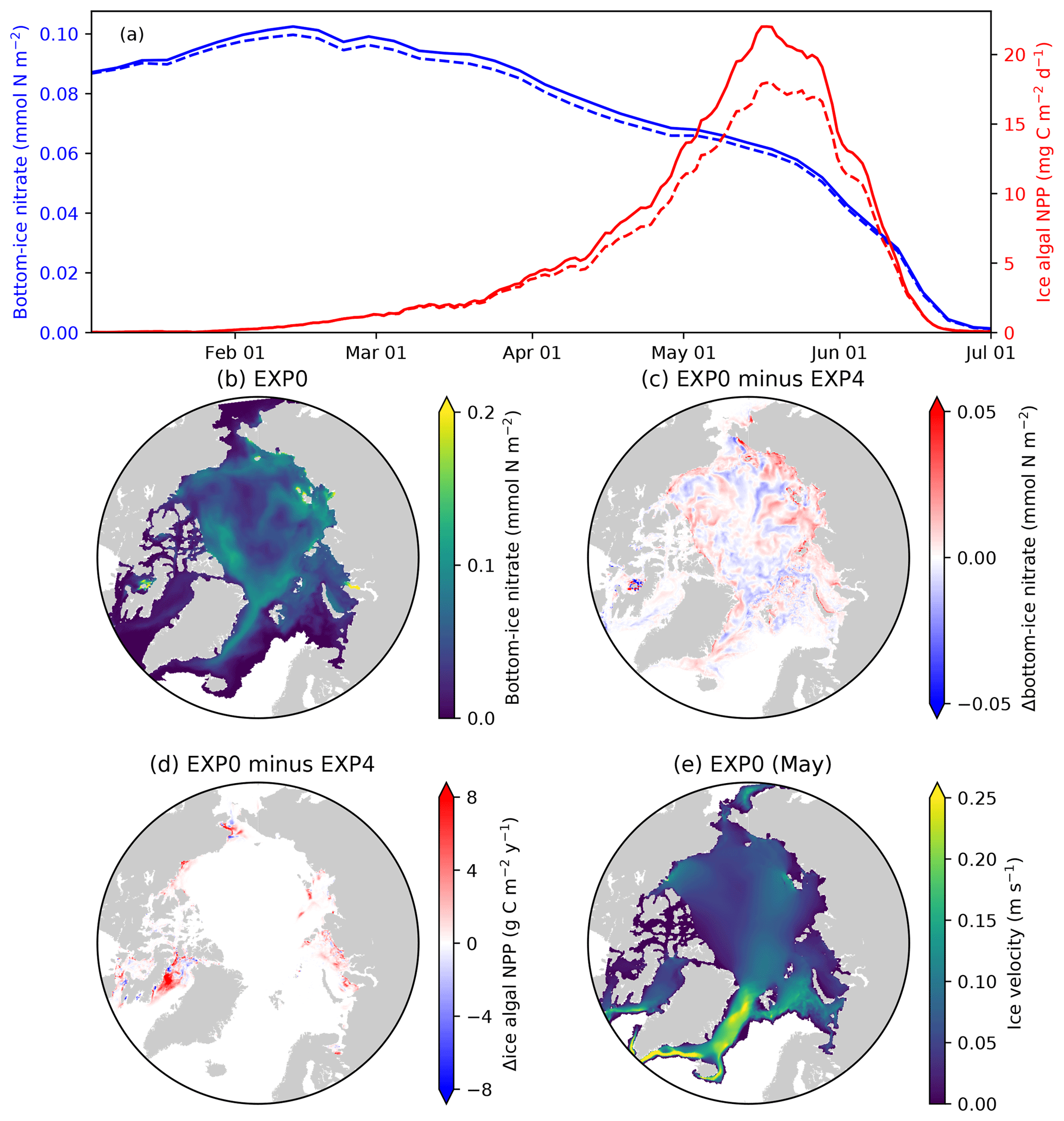
Figure 13Model sensitivity to the horizontal transport of sea-ice biogeochemical state variables. (a) Time series comparison of 5 d mean and pan-Arctic-mean modelled bottom-ice nitrate (blue) and ice algal daily NPP (red) during January–June of 1979 between EXP0 (solid) and EXP4 (dashed). Spatial maps of the annual-mean bottom-ice nitrate in (b) EXP0 and (c) its difference between EXP0 and EXP4, (d) the difference in the ice algal annual NPP between EXP0 and EXP4, and (e) the magnitude of the ice velocity during May.
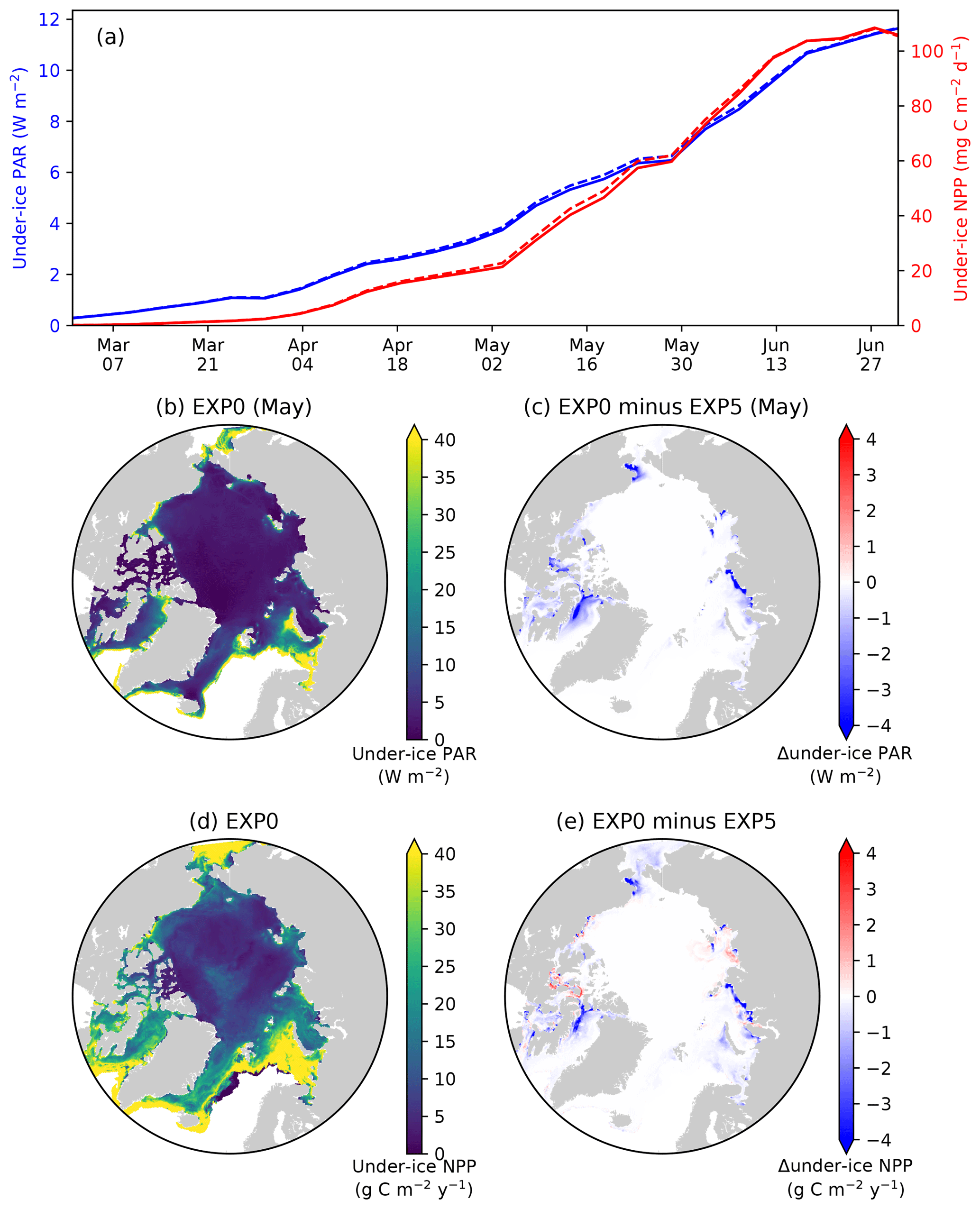
Figure 14Model sensitivity to shading by ice algae. (a) Time series comparison of modelled pan-Arctic-mean and 5 d mean under-ice PAR (blue) and NPP (red) between EXP0 (solid) and EXP5 (dashed) during 1979. Spatial maps of (b) monthly-mean under-ice PAR in May in EXP0 and (c) its difference from EXP5, (d) the under-ice annual NPP in EXP0, and (e) its difference from EXP5.
Two other regional modelling studies prescribe non-zero values of i0 for snow surface. Castellani et al. (2017) set i0 for snow surface to 0.3 based on the measurements over snow-free ice surface (Grenfell and Maykut, 1977). As such, this value (0.3) should be viewed as an overestimate. Similarly, the light penetration through snow is also overestimated in Watanabe et al. (2015), as i0 for snow surface is effectively unity in their study. Using these higher i0 for snow surface reduces light limitation for ice algal growth as long as the formulation for light limitation is inversely proportional to irradiance. However, higher i0 can result in increasing light limitation, e.g., if the formulation assumes some optimal irradiance level with photoinhibition at higher levels, such as done in Watanabe et al. (2015). As such, the overall impact of i0 on ice algal production depends on the choice of formulation and parameter(s) for the light limitation function.
To the best of the authors' knowledge, no studies have ever reported an observed value for i0 for snow surface. For a snow-free ice surface, Grenfell and Maykut (1977) report values ranging between 0.18 and 0.63 depending on both the ice type and whether the incoming shortwave radiation is direct or diffuse. Observation-based estimates of i0 for snow surface would be useful in order to reduce the uncertainty in ice algal and under-ice phytoplankton growth in models.
4.3 Horizontal transport associated with moving sea ice (EXP4)
EXP4 is designed to quantify the contribution of sea-ice advection and diffusion to the overall budget of sea-ice biogeochemical state variables. This analysis can be useful in deciding a location for conducting 1-D simulations in which horizontal processes of sea-ice biogeochemistry are neglected. Specifically, EXP4 is conducted with the identical model formulation as EXP0 except that the advection and diffusion of sea-ice biogeochemical state variables (the effect of horizontal transport associated with moving sea ice) are artificially suppressed (i.e., the first two terms on the right-hand side of Eq. (2) are removed). Note that the advection and diffusion of sea-ice physical state variables are retained in EXP4, so there is no difference in these variables between EXP0 and EXP4.
A time series comparison of the modelled pan-Arctic-mean bottom-ice nitrate and ice algal NPP for 1979 shows that these quantities are always higher in EXP0 than EXP4 (Fig. 13a). The pan-Arctic annual-mean bottom-ice nitrate and the ice algal annual NPP are higher in EXP0 than EXP4 by 2 % and 16 %, respectively. These results indicate that the overall effect of horizontal transport associated with moving sea ice over the pan-Arctic is an increase in these quantities. However, we note that these values could be quite different in other years given the large interannual variability in wind stress fields driving sea-ice drift patterns.
Although the overall effect is an enhancement, the spatial distribution shows regions of local increase and decrease (Fig. 13c–d). The difference in nitrate concentration between the two experiments is relatively high off the west coast of Baffin Island, where the bottom-ice nitrate concentration is relatively high in EXP0 (Fig. 13b), whereas the difference is relatively small on the Canadian Polar Shelf (Fig. 13c). The difference in ice algal NPP is relatively high in regions of high ice algal NPP except for the Canadian Polar Shelf (Fig. 13d), which is a region of relatively slow ice motion (Fig. 13e). One possible explanation for these spatial differences is the horizontal transport of nutrients into regions of high productivity, which results in further increase in ice algal production.
4.4 Shading of ice algae (EXP5)
In EXP5, the shading effect of ice algae on light transfer through the ice is artificially suppressed in order to assess its impact on under-ice NPP. Effectively, this is done by setting the light extinction coefficient for ice algae to zero (Eq. 15 of Mortenson et al., 2017). Note that this modification has no impact on simulated physics. On the pan-Arctic scale, there is almost no effect, as shown in Fig. 14a. The differences in the pan-Arctic- and annual-mean under-ice PAR and the pan-Arctic under-ice annual NPP between EXP0 and EXP5 are 2 % and 1 %, respectively.
Consistent with the patchiness of the ice algal distribution (Fig. 8c), the shading effect is rather localized as shown in Fig. 14b–e. The influence on under-ice PAR is assessed for the month of the ice algal bloom peak (May; Fig. 6c). The spatial distribution of the difference in the under-ice PAR between EXP0 and EXP5 is simply a reflection of ice algal abundance (Fig. 14c). Similarly, a general decrease in the under-ice NPP is found due to shading in the regions of high ice algal production. However, in some regions, shading results in a slight increase in under-ice NPP which is dominated by small phytoplankton, but a slight increase is also seen for large phytoplankton (Fig. 15c). The underlying mechanism for this response of the modelled ecosystem to a perturbation to light is unclear.
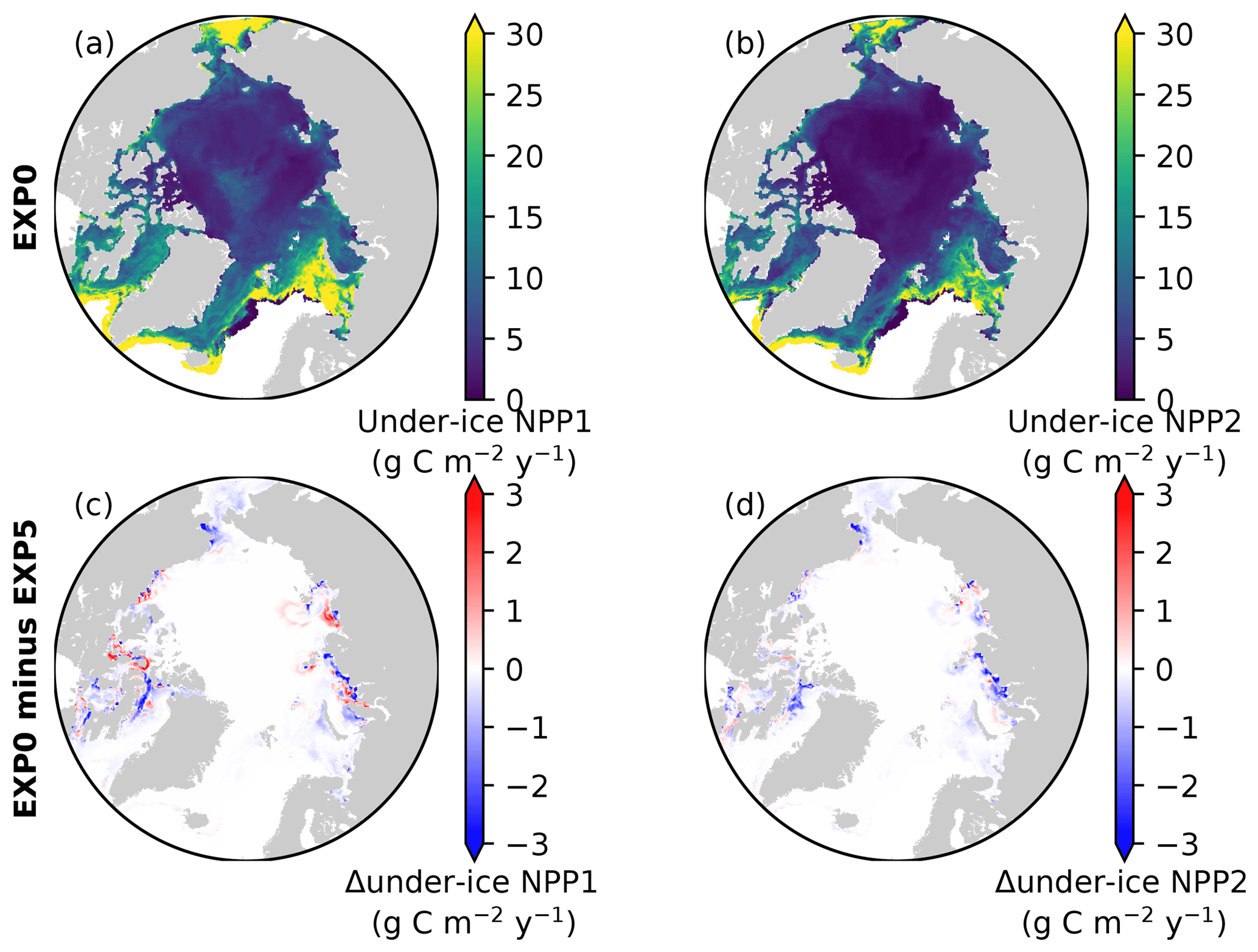
Figure 15Spatial maps of under-ice annual NPP by (a) small and (b) large phytoplankton during 1979 in EXP0, and (c, d) their respective differences from EXP5.
The shading effect of ice algae was recently examined in the model study of Castellani et al. (2017). Their results showed that the effect has greater influence at higher latitudes due to low ambient light. Furthermore, they hypothesized that the onset of the under-ice phytoplankton bloom north of 80∘ N can be delayed by up to 40 d depending on how their modelled under-ice PAR is affected by shading.
It is difficult to directly compare the results of the present study with those of Castellani et al. (2017), primarily due to the difference in the definition of the term under-ice. As described in Sect. 2.5.3, in the present study, a grid cell is considered “under-ice” as long as the ice concentration is 0.15 or above. Because of the high surface albedo and strong light attenuation by snow and ice, the under-ice PAR defined in the present study is therefore dominated by the light through the open-water fraction (see also Dupont, 2012). Consequently, the under-ice NPP is controlled by the light through the open-water fraction and does not show a strong influence by the shading of ice algae. Furthermore, direct comparison is difficult due to the difference in the target year of simulation; Castellani et al. (2017) simulated 2012, while we consider 1979.
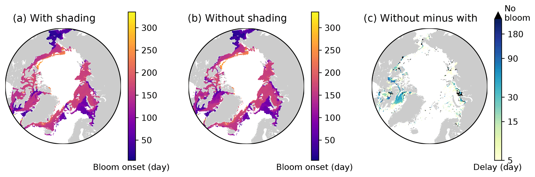
Figure 16Effects of ice algal shading on the onset of under-ice phytoplankton bloom. Spatial maps showing the bloom onset (as the day from 1 January) when the ice algal shading is (a) considered and (b) neglected and (c) the difference between the two cases representing the delay due to the shading in 1979 in EXP0. In panel (c), “No bloom” refers to regions in which the bloom was present in panel (b) but not in panel (a). See Sect. 4.4 for the definition of bloom onset.
Nevertheless, to carry out an analysis comparable to that of Castellani et al. (2017), we calculate the onset of under-ice phytoplankton bloom as follows. A bloom onset is defined as the day when bottom-ice PAR exceeds 0.4 W m−2 and remains above this value at least for 30 d. This threshold for bottom-ice PAR corresponds to the limit for under-ice algal growth considered in Castellani et al. (2017), assuming a unit conversion (from µmol photon m−2 s−1 to W m−2) factor of 1∕4.56 (Lavoie et al., 2005). Figure 16 shows the spatial variability in the under-ice bloom onset based on the definition above. The bloom takes place mostly in seasonally ice-covered regions, while it is absent in most of the pack ice (as indicated by white regions). Unlike Castellani et al. (2017), the under-ice bloom north of 80∘ N is absent even without the shading effect. The absence of the bloom in our simulation is due to the presence of snow in this region; despite the extremely low quantity (<0.01 m; data not shown), it keeps the light level below the threshold for the bloom to occur. The median value of the onset is on the 155th day (June 6) when the shading is accounted for (Fig. 16a), while it is 10 d earlier without the shading effect (Fig. 16b). Note that these results are based on the analysis of modelled light transmission through snow and ice columns only, and therefore are not comparable to field observations of under-ice blooms triggered by light transmission through open leads (e.g., Assmy et al., 2017).
Figure 16c shows the spatial variability in the delay in the under-ice bloom onset caused by the ice algal shading. The values range from 5 to 275 d; in some places, the bloom is prevented completely. The present study does confirm the finding of Castellani et al. (2017) that the shading effect is spatially variable and can have a strong impact on the phytoplankton bloom timing under the ice with high ice algal biomass. However, given the patchiness of ice algal distribution (mostly confined to shelf regions) and the control of the light through the open-water fraction, the impact of the shading on the pan-Arctic under-ice annual NPP is negligible.
Besides the shading effect, ice algae can contribute to ice melting through light absorption and conversion to heat (Zeebe et al., 1996). However, our model does not incorporate this bio-physical coupling for simplicity. Kauko et al. (2017) estimated that up to 0.8 cm of bottom ice was melted by ice algae and other particles in a week. Zeebe et al. (1996) showed that the amount of melting is highly sensitive to the amount of solar radiation, the ice algal biomass, and its vertical extent. Furthermore, Lavoie et al. (2005) quantified the impact on ice algal loss (release into the water column), and found that the loss is highly sensitive to the amount of solar radiation and ice algal biomass, but not so to the photosynthetic efficiency of ice algae. Future model studies can assess the impact on under-ice blooms, and eventually the combined effect of both the shading and melting by ice algae.
In the present study, we have developed a sea-ice biogeochemistry model which is coupled to NEMO. A number of modifications to the sea-ice physical model used in the standard distribution of NEMO (LIM2), to the ocean biogeochemical model (CanOE), and to the existing pan-Arctic configuration (NAA) were necessary to properly simulate the physical and biogeochemical processes in ice-covered regions. Results of the reference simulation (EXP0) were discussed and compared with previous studies, with a focus on the year 1979; more thorough evaluation of the model performance over the recent decades is planned for future studies. Adopting a high vertical resolution in the upper water column was found to be necessary to properly represent the effects of a meltwater lens on surface nutrients and the formation of a subsurface chlorophyll maximum. Furthermore, the vertical resolution was shown to have an effect on the magnitude of the modelled surface seawater DMS concentration (∼10 % annually and up to ∼20 % seasonally), which in turn influences DMS emissions. Results of the sensitivity experiments demonstrated that LIM2 requires high-frequency (daily) snowfall forcing data to simulate realistic snow depth (EXP1 and 2); the assumption of no light penetration through snow in LIM2 is unrealistic for simulating an adequate ice algal bloom (EXP3); horizontal transport of sea ice contributes to an enhancement of the pan-Arctic ice algal annual NPP by 16 % (EXP4); and attenuation of light by ice algae has local influence on under-ice NPP but is negligible when estimating larger-scale quantities (e.g., pan-Arctic under-ice annual NPP) (EXP5). While we believe that these findings would be qualitatively similar in other years, it would be worthwhile to quantify their interannual variability. The modifications to LIM2, CanOE, and NAA adopted in the present study are also applicable to other sub-models and configurations of NEMO (e.g., LIM3, PISCES, ORCA) as the code structures are similar, and therefore can be incorporated into future pan-Arctic biogeochemical studies. The sea-ice biogeochemical model developed in the present study has been embedded into NEMO in a generic way (see Appendix A), and can therefore be easily coupled to the aforementioned sub-models. To our knowledge, such a development has not been done previously within NEMO. Further sensitivity experiments and observational constraints are needed to refine the important parameters (e.g., i0) for sea-ice biogeochemistry.
The model code and the configuration used for conducting model simulations are archived at the Zenodo repository https://doi.org/10.5281/zenodo.1435254 (Hayashida, 2018b).
Figure A1 shows the structure of the NEMO v3.4 source-code directory (NEMO), which includes the following subdirectories (sub-models): OPA_SRC (OPA), LIM_SRC_2 (LIM2), and TOP_SRC (ocean biogeochemistry). The directory TOP_SRC contains two subdirectories: PISCES and MY_TRC. In this study, the directory PISCES contains the source code of CanOE, as CanOE has been developed using the code structure of the PISCES ocean biogeochemical model. The other directory, MY_TRC, consists of a list of generic modules that can be modified by end users to add their own biogeochemical models; we introduced an ocean sulfur cycle and sea-ice biogeochemistry into this interface. Furthermore, we modified a few modules in the directories LIM_SRC_2 and PISCES for the implementation of sea-ice biogeochemistry into the NEMO modelling system (Table A1).
Numerically, the tendencies for the sea-ice biogeochemical state variables are computed at each time step as follows: first, the concentrations of all state variables from the previous time step are transferred from the module trcsms_my_trc.F90 to the module limtrp_2.F90 to compute the advective and diffusive tendencies. The updated concentrations are transferred back to the module trcsms_my_trc.F90 within which the biological and chemical sources and sinks as well as the ice–ocean fluxes of these state variables are computed.
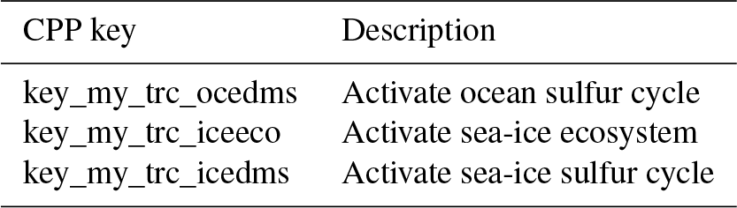
In NEMO, user-specific modules built within MY_TRC are designed to be activated by defining the C preprocessor (CPP) key key_my_trc. As such, we assigned CPP keys for each component of the newly developed models, which can be activated as needed (Table A2).
Table A1A list of NEMO modules modified to add ocean sulfur cycle and sea-ice biogeochemistry.
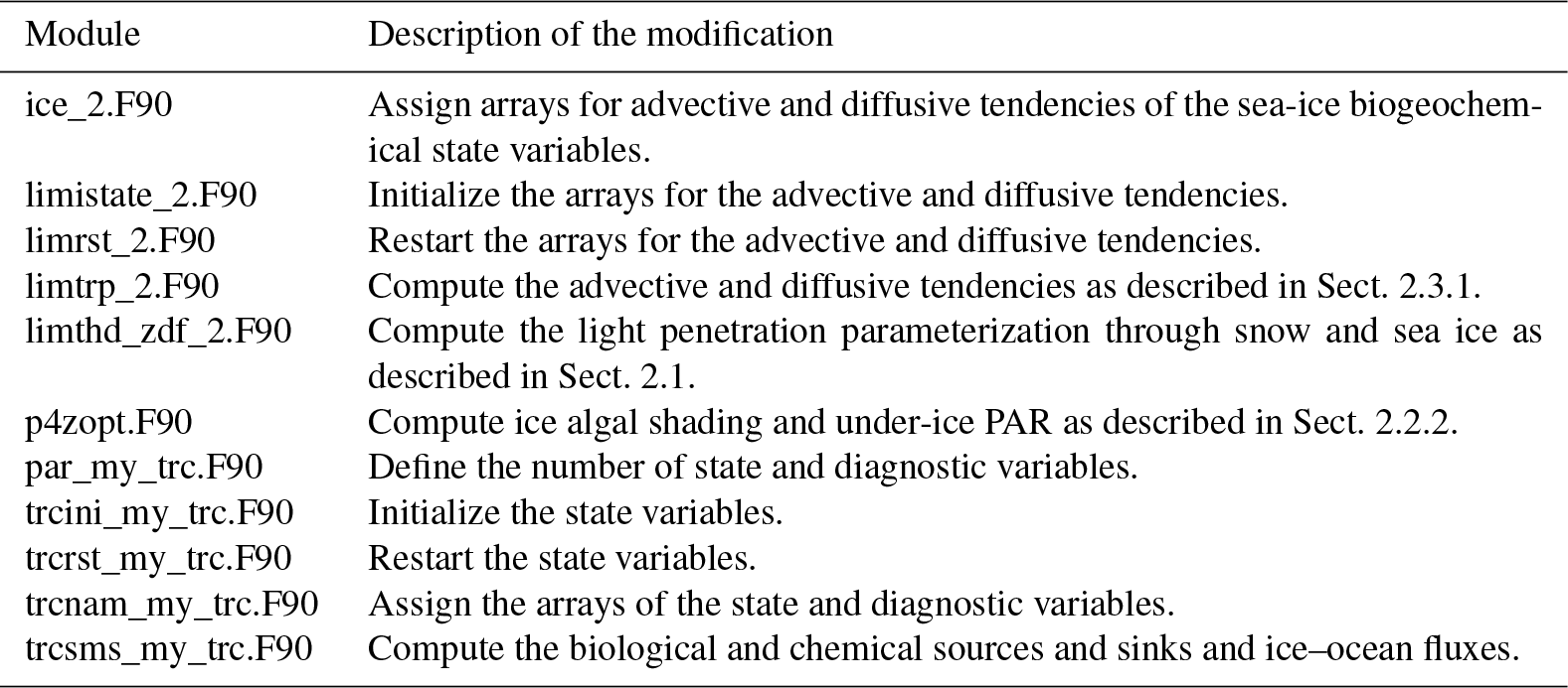
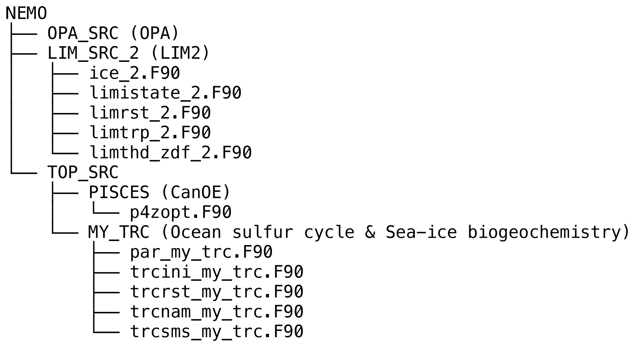
Figure A1File tree diagram of the OPA–LIM2–CanOE configuration of NEMO v3.4. The modules listed in the diagram (*.F90) have been modified in order to implement ocean sulfur cycle and sea-ice biogeochemistry into the present configuration.
The annual-mean time series of modelled snow and ice volumes, ice extent, seawater nitrate, and ice algal and phytoplankton biomass over the 11 years of EXP0 are shown in Fig. B1. This time period can be considered sufficiently long enough to spin up some of these quantities, while others may require additional time to spin-up. However, none of these quantities reach a steady state in the current setup as the model was driven by interannual surface and lateral boundary conditions. The aim of the present analysis is to examine the temporal variability starting from the initial year and compare with findings of previous model studies. Presenting the results from the initial year is often neglected in the literature, but can be useful for future studies.
The annual-mean modelled snow volume stabilizes around 0.8×10³ km3 after an initial drop of about 0.1×10³ km3 from year 1969 to 1970 (Fig. B1a), indicating a spin-up period of a year or so. In contrast, the annual-mean modelled ice volume variations show an initial reduction during 1969–1971 followed by an overall increase during 1973–1979. The relatively short duration of this simulation does not allow us to distinguish between trends and slow interannual variability, so we cannot determine if the ice volume has spun up based solely on this analysis; this will be addressed in a follow up study. A previous pan-Arctic regional model study of Watanabe (2013) shows a spin-up period of 10 years for modelled ice volume based on a simulation using a fixed annual cycle of atmospheric forcing and restoring of temperature and salinity.

Figure B1Time series of annual-mean modelled (a) snow and ice volumes, (b) ice extent and depth-integrated (90 m) seawater nitrate concentration, and (c) depth-integrated (3 cm) ice algal NPP and depth-integrated (90 m) phytoplankton NPP in EXP0. The depth-integrated quantities represent averages over the entire model domain.
Modelled ice extent shows a decrease in the first 6 years followed by a stabilization in the last 5 years, suggesting that this quantity spun up at year 1975 (Fig. B1b). This spin-up time is similar to that found in the pan-Arctic model study of Jin et al. (2012), in which their modelled ice area and extent became comparable to the observations after the first 6 years of simulation.
Annual-mean modelled seawater nitrate concentration integrated over the upper 90 m of the water column shows both increases and decreases during the 11 years (Fig. B1b), although the size of the fluctuation (∼20 mmol N m−2) is small relative to its mean state (∼490 mmol N m−2). Similarly to ice volume, a longer simulation would be needed to distinguish between trends and interannual variability in the modelled nitrate concentration. A previous pan-Arctic model study of Dupont (2012) indicated a spin-up period of at least a decade for nitrate in the upper 100 m water column for the model domain he considered. The modelled primary producers (ice algae and phytoplankton) appear to have spun up within a year of the model simulation, as their annual primary production fluctuates around a steady mean following the first year (Fig. B1c).
The model simulates subsurface chlorophyll a maxima (SCMs) at various locations in the Arctic. Figure C1 shows an example for the Chukchi Sea where the SCM is formed at depth in mid-June. This SCM depth (>20 m) is comparable to observations (e.g., Brown et al., 2015). A detailed discussion on SCM simulated by CanOE will be provided in a future study (Steiner et al., 2019).
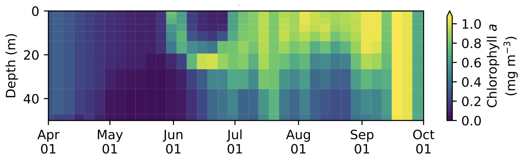
Figure C1Vertical time series of modelled 5 d mean chlorophyll a concentration in the upper 50 m of the water column at the grid cell corresponding to 170∘ W and 70∘ N in the Chukchi Sea.
Here we demonstrate that the lack of snow accumulation using the daily climatology for snowfall dataset can be resolved by tuning the model parameter nn_fsbc, which defines the frequency of the computation of surface boundary conditions and sea-ice physics relative to that of ocean dynamics. Figure D1 compares the annual-mean modelled snow depths for year 1970 of EXP2 with those of the simulations that varied nn_fsbc from the default value of 1 (i.e., the time step for surface boundary condition and sea-ice physics is identical to the ocean time step) to 5 and 10 (i.e., surface boundary condition and sea-ice physics are computed at every 5 and 10 ocean time steps, respectively). We find that setting nn_fsbc to 5 or 10 increased the modelled snow depth quite remarkably (Fig. D1). This high sensitivity to the choice of nn_fsbc is somewhat unexpected given that the tested range (1–10 time steps, equivalent to 20–200 min) is far less than the temporal resolution of the CORE-II dataset. A more detailed analysis of the model sensitivity to nn_fsbc is outside the scope of this study. Furthermore, we note that the tuning of this parameter without known constraints is quite arbitrary and might have other implications for modelled dynamics. As discussed in the main text, the usage of high-frequency atmospheric forcing dataset is therefore recommended to realistically simulate snow accumulation.
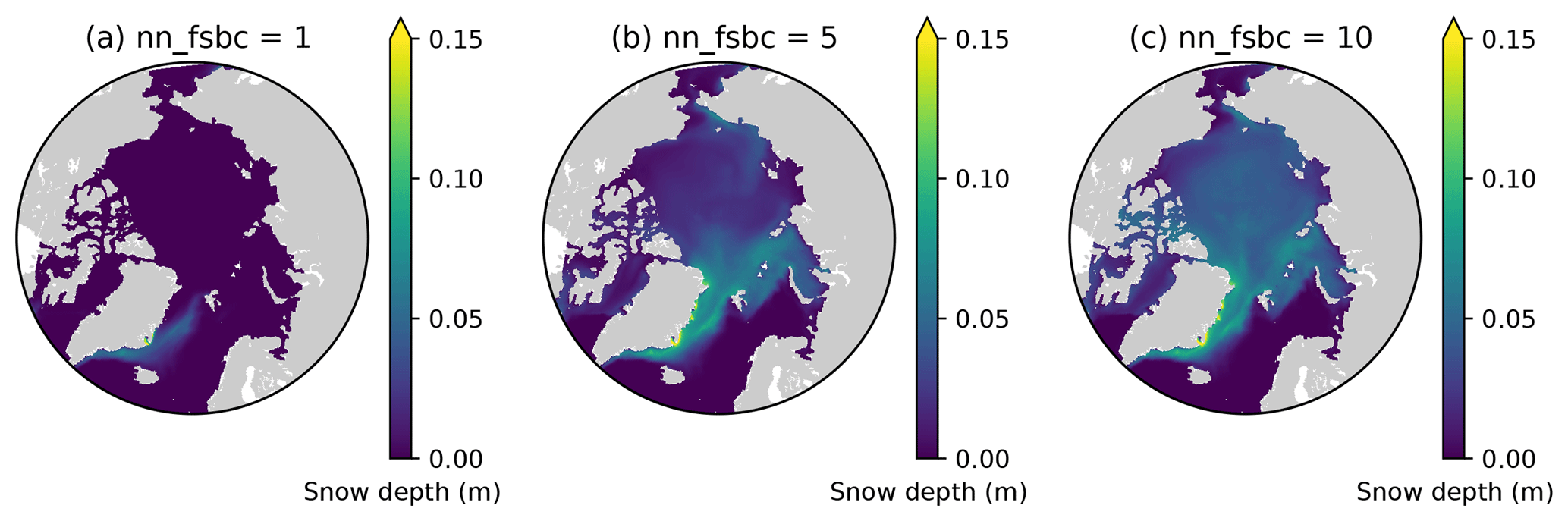
Figure D1Sensitivity of modelled snow depth to the parameter nn_fsbc, which defines the frequency of the computation of surface boundary conditions and sea-ice physics relative to that of ocean dynamics. Spatial distribution of annual-mean modelled snow depth for 1970 when nn_fsbc is set to (a) 1, (b) 5, and (c) 10.
The supplement related to this article is available online at: https://doi.org/10.5194/gmd-12-1965-2019-supplement.
HH wrote the model code, designed and performed the numerical experiments, conducted the analysis, and wrote the paper with input from JRC, AMH, XH, AHM, EM, PGM, OGJR, TS, and NSS. AHM and NSS supervised the project.
The authors declare that they have no conflict of interest.
We thank Achim Randelhoff and two anonymous referees for their thorough review, which greatly improved the presentation of this paper. We thank Martin Vancoppenolle for helpful discussion on the LIM model. This study contributes to the SCOR working group on Biogeochemical Exchange Processes at Sea Ice Interfaces (BEPSII), the Network on Climate and Aerosols: Addressing Key Uncertainties in Remote Canadian Environments (NETCARE), and ArcticNet. This research was enabled in part by support provided by WestGrid and Compute Canada. We thank Belaid Moa (University of Victoria) for computational support, Arlan Dirkson (Université du Québec à Montréal) for providing a netCDF version of the PIOMAS monthly-mean ice thickness and concentration gridded data products, Clark Pennelly (University of Alberta) for providing a modified version of the DFS dataset, and Ken Denman for providing a helpful discussion on growth rates and primary productivity. The original NAA configuration was developed under an NSERC Discovery Grant award to PGM.
This research has been supported by the Natural Sciences and Engineering Research Council (NETCARE), ArcticNet, Fisheries and Oceans Canada, and Environment and Climate Change Canada.
This paper was edited by Andrew Yool and reviewed by Achim Randelhoff and two anonymous referees.
Abraham, C., Steiner, N., Monahan, A., and Michel, C.: Effects of subgrid-scale snow thickness variability on radiative transfer in sea ice, J. Geophys. Res.-Oceans, 120, 5597–5614, https://doi.org/10.1002/2015JC010741, 2015. a
Amante, C. and Eakins, B. W.: ETOPO1 1 arc-minute global relief model: procedures, data sources and analysis, US Department of Commerce, National Oceanic and Atmospheric Administration, National Environmental Satellite, Data, and Information Service, National Geophysical Data Center, Marine Geology and Geophysics Division Colorado, Boulder, Colorado, USA, 2009. a
Arora, V. K., Scinocca, J. F., Boer, G. J., Christian, J. R., Denman, K. L., Flato, G. M., Kharin, V. V., Lee, W. G., and Merryfield, W. J.: Carbon emission limits required to satisfy future representative concentration pathways of greenhouse gases, Geophys. Res. Lett., 38, L05805, https://doi.org/10.1029/2010GL046270, 2011. a
Arrigo, K. R.: Sea Ice Ecosystems, Annu. Rev. Mar. Sci., 6, 439–467, https://doi.org/10.1146/annurev-marine-010213-135103, 2014. a
Arrigo, K. R., Sullivan, C. W., and Kremer, J. N.: A bio-optical model of Antarctic sea ice, J. Geophys. Res.-Oceans, 96, 10581–10592, https://doi.org/10.1029/91JC00455, 1991. a
Assmy, P., Ehn, J. K., Fernández-Méndez, M., Hop, H., Katlein, C., Sundfjord, A., Bluhm, K., Daase, M., Engel, A., Fransson, A., Granskog, M. A., Hudson, S. R., Kristiansen, S., Nicolaus, M., Peeken, I., Renner, A. H. H., Spreen, G., Tatarek, A., and Wiktor, J.: Floating Ice-Algal Aggregates below Melting Arctic Sea Ice, PLoS ONE, 8, e76599, https://doi.org/10.1371/journal.pone.0076599, 2013. a
Assmy, P., Fernández-Méndez, M., Duarte, P., Meyer, A., Randelhoff, A., Mundy, C. J., Olsen, L. M., Kauko, H. M., Bailey, A., Chierici, M., Cohen, L., Doulgeris, A. P., Ehn, J. K., Fransson, A., Gerland, S., Hop, H., Hudson, S. R., Hughes, N., Itkin, P., Johnsen, G., King, J. A., Koch, B. P., Koenig, Z., Kwasniewski, S., Laney, S. R., Nicolaus, M., Pavlov, A. K., Polashenski, C. M., Provost, C., Rösel, A., Sandbu, M., Spreen, G., Smedsrud, L. H., Sundfjord, A., Taskjelle, T., Tatarek, A., Wiktor, J., Wagner, P. M., Wold, A., Steen, H., and Granskog, M. A.: Leads in Arctic pack ice enable early phytoplankton blooms below snow-covered sea ice, Sci. Rep., 7, 40850, https://doi.org/10.1038/srep40850, 2017. a
Aumont, O., Ethé, C., Tagliabue, A., Bopp, L., and Gehlen, M.: PISCES-v2: an ocean biogeochemical model for carbon and ecosystem studies, Geosci. Model Dev., 8, 2465–2513, https://doi.org/10.5194/gmd-8-2465-2015, 2015. a, b
Balmaseda, M. A., Mogensen, K., and Weaver, A. T.: Evaluation of the ECMWF ocean reanalysis system ORAS4, Q. J. Roy. Meteor. Soc., 139, 1132–1161, https://doi.org/10.1002/qj.2063, 2013. a
Bouillon, S., Maqueda, M. A. M., Legat, V., and Fichefet, T.: An elastic–viscous–plastic sea ice model formulated on Arakawa B and C grids, Ocean Model., 27, 174–184, 2009. a
Brown, Z. W., Lowry, K. E., Palmer, M. A., van Dijken, G. L., Mills, M. M., Pickart, R. S., and Arrigo, K. R.: Characterizing the subsurface chlorophyll a maximum in the Chukchi Sea and Canada Basin, Deep-Sea Res. Pt. II, 118, 88–104, https://doi.org/10.1016/j.dsr2.2015.02.010, 2015. a, b
Castellani, G., Losch, M., Lange, B. A., and Flores, H.: Modeling Arctic sea-ice algae: Physical drivers of spatial distribution and algae phenology, J. Geophys. Res.-Oceans, 122, 7466–7487, https://doi.org/10.1002/2017JC012828, 2017. a, b, c, d, e, f, g, h, i
Crank, J. and Nicolson, P.: A practical method for numerical evaluation of solutions of partial differential equations of the heat-conduction type, Adv. Comput. Math., 6, 207–226, https://doi.org/10.1007/BF02127704, 1996. a
Christian, J. R., et al.: The Canadian Ocean Ecosystem Model (CanOE): a new ocean biogeochemistry model based on the NEMO modelling system, in preparation, 2019. a, b, c
Dai, A. and Trenberth, K. E.: Estimates of Freshwater Discharge from Continents: Latitudinal and Seasonal Variations, J. Hydrometeorol., 3, 660–687, https://doi.org/10.1175/1525-7541(2002)003<0660:EOFDFC>2.0.CO;2, 2002. a
Deal, C., Jin, M., Elliott, S., Hunke, E., Maltrud, M., and Jeffery, N.: Large-scale modeling of primary production and ice algal biomass within arctic sea ice in 1992, J. Geophys. Res., 116, C07004, https://doi.org/10.1029/2010JC006409, 2011. a, b, c, d, e
Dee, D. P., Uppala, S. M., Simmons, A. J., Berrisford, P., Poli, P., Kobayashi, S., Andrae, U., Balmaseda, M. A., Balsamo, G., Bauer, P., Bechtold, P., Beljaars, A. C. M., van de Berg, L., Bidlot, J., Bormann, N., Delsol, C., Dragani, R., Fuentes, M., Geer, A. J., Haimberger, L., Healy, S. B., Hersbach, H., Hólm, E. V., Isaksen, L., Kållberg, P., Köhler, M., Matricardi, M., McNally, A. P., Monge-Sanz, B. M., Morcrette, J.-J., Park, B.-K., Peubey, C., de Rosnay, P., Tavolato, C., Thépaut, J.-N., and Vitart, F.: The ERA-Interim reanalysis: configuration and performance of the data assimilation system, Q. J. Roy. Meteor. Soc., 137, 553–597, https://doi.org/10.1002/qj.828, 2011. a
Dupont, F.: Impact of sea-ice biology on overall primary production in a biophysical model of the pan-Arctic Ocean, J. Geophys. Res.-Oceans, 117, C00D17, https://doi.org/10.1029/2011JC006983, 2012. a, b, c, d, e, f, g, h, i, j, k
Dupont, F., Higginson, S., Bourdallé-Badie, R., Lu, Y., Roy, F., Smith, G. C., Lemieux, J.-F., Garric, G., and Davidson, F.: A high-resolution ocean and sea-ice modelling system for the Arctic and North Atlantic oceans, Geosci. Model Dev., 8, 1577–1594, https://doi.org/10.5194/gmd-8-1577-2015, 2015. a
Dussin, R., Barnier, B., Brodeau, L., and Molines, J. M.: The making of the Drakkar Forcing Set DFS5, DRAKKAR/MyOcean Rep. 01–04, 16, Laboratoire de glaciologie et géophysique de l'environnement (LGGE), Grenoble, France, 2016. a, b, c
Eppley, R. W.: Temperature and phytoplankton growth in the sea, Fish. Bull., 70, 1063–1085, 1972. a
Fichefet, T. and Maqueda, M. A. M.: Sensitivity of a global sea ice model to the treatment of ice thermodynamics and dynamics, J. Geophys. Res.-Oceans, 102, 12609–12646, https://doi.org/10.1029/97JC00480, 1997. a
Flato, G. M. and Brown, R. D.: Variability and climate sensitivity of landfast Arctic sea ice, J. Geophys. Res.-Oceans, 101, 25767–25777, https://doi.org/10.1029/96JC02431, 1996. a
Garcia, H. E., Locarnini, R. A., Boyer, T. P., Antonov, J. I., Baranova, O. K., Zweng, M. M., Reagan, J. R., and Johnson, D. R.: World Ocean Atlas 2013, Volume 3: Dissolved Oxygen, Apparent Oxygen Utilization, and Oxygen Saturation, edited by: Levitus, S. and Mishonov, A., NOAA Atlas NESDIS 75, National Oceanographic Data Center, Maryland, USA, 27 pp., 2014. a
Garrison, D. L., Ackley, S. F., and Buck, K. R.: A physical mechanism for establishing algal populations in frazil ice, Nature, 306, 363–365, https://doi.org/10.1038/306363a0, 1983. a
Grenfell, T. C. and Maykut, G. A.: The optical properties of ice and snow in the Arctic Basin, J. Glaciol., 18, 445–463, 1977. a, b, c, d
Hashimoto, S., Horimoto, N., Yamaguchi, Y., Ishimaru, T., and Saino, T.: Relationship between net and gross primary production in the Sagami Bay, Japan, Limnol. Oceanogr., 50, 1830–1835, 2005. a
Hayashida, H.: Modelling sea-ice and oceanic dimethylsulfide production and emissions in the Arctic, PhD Thesis, University of Victoria, Victoria, BC, Canada, available at: https://dspace.library.uvic.ca//handle/1828/10486 (last access: 5 January 2019), 2018a. a, b, c, d
Hayashida, H.: CSIB v1 source code (Version v1), Zenodo, https://doi.org/10.5281/zenodo.1435254, 2018b. a
Hayashida, H., Steiner, N., Monahan, A., Galindo, V., Lizotte, M., and Levasseur, M.: Implications of sea-ice biogeochemistry for oceanic production and emissions of dimethyl sulfide in the Arctic, Biogeosciences, 14, 3129–3155, https://doi.org/10.5194/bg-14-3129-2017, 2017. a, b, c, d, e
Hu, X. and Myers, P. G.: A Lagrangian view of Pacific water inflow pathways in the Arctic Ocean during model spin-up, Ocean Model., 71, 66–80, https://doi.org/10.1016/j.ocemod.2013.06.007, 2013. a, b, c, d, e, f
Hu, X. and Myers, P. G.: Changes to the Canadian Arctic Archipelago Sea Ice and Freshwater Fluxes in the Twenty-First Century under the Intergovernmental Panel on Climate Change A1B Climate Scenario, Atmos.-Ocean, 52, 331–350, https://doi.org/10.1080/07055900.2014.942592, 2014. a
Jin, M., Deal, C. J., Wang, J., Shin, K.-H., Tanaka, N., Whitledge, T. E., Lee, S. H., and Gradinger, R. R.: Controls of the landfast ice–ocean ecosystem offshore Barrow, Alaska, Ann. Glaciol., 44, 63–72, 2006. a
Jin, M., Deal, C., Lee, S. H., Elliott, S., Hunke, E., Maltrud, M., and Jeffery, N.: Investigation of Arctic sea ice and ocean primary production for the period 1992–2007 using a 3-D global ice–ocean ecosystem model, Deep-Sea Res. Pt. II, 81–84, 28–35, https://doi.org/10.1016/j.dsr2.2011.06.003, 2012. a, b, c, d, e, f, g, h, i, j, k, l
Jin, M., Popova, E. E., Zhang, J., Ji, R., Pendleton, D., Varpe, Ø., Yool, A., and Lee, Y. J.: Ecosystem model intercomparison of under-ice and total primary production in the Arctic Ocean, J. Geophys. Res.-Oceans, 121, 934–948, https://doi.org/10.1002/2015JC011183, 2015. a
Jin, M., Deal, C., Maslowski, W., Matrai, P., Roberts, A., Osinski, R., Lee, Y. J., Frants, M., Elliott, S., Jeffery, N., Hunke, E., and Wang, S.: Effects of Model Resolution and Ocean Mixing on Forced Ice-Ocean Physical and Biogeochemical Simulations Using Global and Regional System Models, J. Geophys. Res.-Oceans, 123, 358–377, https://doi.org/10.1002/2017JC013365, 2018. a, b, c, d
Kauko, H. M., Taskjelle, T., Assmy, P., Pavlov, A. K., Mundy, C. J., Duarte, P., Fernández-Méndez, M., Olsen, L. M., Hudson, S. R., Johnsen, G., Elliott, A., Wang, F., and Granskog, M. A.: Windows in Arctic sea ice: Light transmission and ice algae in a refrozen lead, J. Geophys. Res.-Biogeo., 122, 2016JG003626, https://doi.org/10.1002/2016JG003626, 2017. a
Lauvset, S. K., Key, R. M., Olsen, A., van Heuven, S., Velo, A., Lin, X., Schirnick, C., Kozyr, A., Tanhua, T., Hoppema, M., Jutterström, S., Steinfeldt, R., Jeansson, E., Ishii, M., Perez, F. F., Suzuki, T., and Watelet, S.: A new global interior ocean mapped climatology: the GLODAP version 2, Earth Syst. Sci. Data, 8, 325–340, https://doi.org/10.5194/essd-8-325-2016, 2016. a
Lavoie, D., Denman, K., and Michel, C.: Modeling ice algal growth and decline in a seasonally ice-covered region of the Arctic (Resolute Passage, Canadian Archipelago), J. Geophys. Res., 110, C11009, https://doi.org/10.1029/2005JC002922, 2005. a, b, c
Legendre, L., Ackley, S. F., Dieckmann, G. S., Gulliksen, B., Horner, R., Hoshiai, T., Melnikov, I. A., Reeburgh, W. S., Spindler, M., and Sullivan, C. W.: Ecology of sea ice biota, Polar Biol., 12, 429–444, https://doi.org/10.1007/BF00243114, 1992. a, b, c
Leu, E., Mundy, C. J., Assmy, P., Campbell, K., Gabrielsen, T. M., Gosselin, M., Juul-Pedersen, T., and Gradinger, R.: Arctic spring awakening – Steering principles behind the phenology of vernal ice algal blooms, Prog. Oceanogr., 139, 151–170, https://doi.org/10.1016/j.pocean.2015.07.012, 2015. a
Loose, B., McGillis, W. R., Schlosser, P., Perovich, D., and Takahashi, T.: Effects of freezing, growth, and ice cover on gas transport processes in laboratory seawater experiments, Geophys. Res. Lett., 36, L05603, https://doi.org/10.1029/2008GL036318, 2009. a
Madec, G.: NEMO ocean engine, Tech. Rep. 27, Institut Pierre Simon Laplace (ISPL), France, 2008. a, b, c
Maykut, G. A. and Untersteiner, N.: Some results from a time-dependent thermodynamic model of sea ice, J. Geophys. Res., 76, 1550–1575, https://doi.org/10.1029/JC076i006p01550, 1971. a
Melnikov, I. A., Kolosova, E. G., Welch, H. E., and Zhitina, L. S.: Sea ice biological communities and nutrient dynamics in the Canada Basin of the Arctic Ocean, Deep-Sea Res. Pt. I, 49, 1623–1649, https://doi.org/10.1016/S0967-0637(02)00042-0, 2002. a
Miller, L. A., Fripiat, F., Else, B. G., Bowman, J. S., Brown, K. A., Collins, R. E., Ewert, M., Fransson, A., Gosselin, M., Lannuzel, D., Meiners, K. M., Michel, C., Nishioka, J., Nomura, D., Papadimitriou, S., Russell, L. M., Sørensen, L. L., Thomas, D. N., Tison, J.-L., van Leeuwe, M. A., Vancoppenolle, M., Wolff, E. W., and Zhou, J.: Methods for biogeochemical studies of sea ice: The state of the art, caveats, and recommendations, Elementa, 3, 38, https://doi.org/10.12952/journal.elementa.000038, 2015. a
Morel, A.: Optical modeling of the upper ocean in relation to its biogenous matter content (case I waters), J. Geophys. Res.-Oceans, 93, 10749–10768, https://doi.org/10.1029/JC093iC09p10749, 1988. a
Mortenson, E., Hayashida, H., Steiner, N., Monahan, A., Blais, M., Gale, M. A., Galindo, V., Gosselin, M., Hu, X., Lavoie, D., and Mundy, C. J.: A model-based analysis of physical and biological controls on ice algal and pelagic primary production in Resolute Passage, Elem. Sci. Anth., 5, 39, https://doi.org/10.1525/elementa.229, 2017. a, b, c, d, e, f
Olsen, L. M., Laney, S. R., Duarte, P., Kauko, H. M., Fernández-Méndez, M., Mundy, C. J., Rösel, A., Meyer, A., Itkin, P., Cohen, L., Peeken, I., Tatarek, A., Róźańska-Pluta, M., Wiktor, J., Taskjelle, T., Pavlov, A. K., Hudson, S. R., Granskog, M. A., Hop, H., and Assmy, P.: The seeding of ice algal blooms in Arctic pack ice: The multiyear ice seed repository hypothesis, J. Geophys. Res.-Biogeo., 122, 2016JG003668, https://doi.org/10.1002/2016JG003668, 2017. a
Pabi, S., van Dijken, G. L., and Arrigo, K. R.: Primary production in the Arctic Ocean, 1998–2006, J. Geophys. Res.-Oceans, 113, C08005, https://doi.org/10.1029/2007JC004578, 2008. a
Popova, E. E., Yool, A., Coward, A. C., Dupont, F., Deal, C., Elliott, S., Hunke, E., Jin, M., Steele, M., and Zhang, J.: What controls primary production in the Arctic Ocean? Results from an intercomparison of five general circulation models with biogeochemistry, J. Geophys. Res.-Oceans, 117, C00D12, https://doi.org/10.1029/2011JC007112, 2012. a, b
Prather, M. J.: Numerical advection by conservation of second-order moments, J. Geophys. Res.-Atmos., 91, 6671–6681, https://doi.org/10.1029/JD091iD06p06671, 1986. a
Rampal, P., Weiss, J., Marsan, D., and Bourgoin, M.: Arctic sea ice velocity field: General circulation and turbulent-like fluctuations, J. Geophys. Res.-Oceans, 114, C10014, https://doi.org/10.1029/2008JC005227, 2009. a
Rampal, P., Bouillon, S., Bergh, J., and Ólason, E.: Arctic sea-ice diffusion from observed and simulated Lagrangian trajectories, The Cryosphere, 10, 1513–1527, https://doi.org/10.5194/tc-10-1513-2016, 2016. a
Rebreanu, L., Vanderborght, J.-P., and Chou, L.: The diffusion coefficient of dissolved silica revisited, Mar. Chem., 112, 230–233, https://doi.org/10.1016/j.marchem.2008.08.004, 2008. a
Roy, F., Chevallier, M., Smith, G. C., Dupont, F., Garric, G., Lemieux, J.-F., Lu, Y., and Davidson, F.: Arctic sea ice and freshwater sensitivity to the treatment of the atmosphere-ice-ocean surface layer: THE ARCTIC AIR-ICE-OCEAN SURFACE LAYER, J. Geophys. Res.-Oceans, 120, 4392–4417, https://doi.org/10.1002/2014JC010677, 2015. a
Sakshaug, E.: Primary and Secondary Production in the Arctic Seas, in: The Organic Carbon Cycle in the Arctic Ocean, edited by: Stein, R. and MacDonald, R. W., Springer Berlin Heidelberg, 57–81, https://doi.org/10.1007/978-3-642-18912-8_3, 2004. a
Sakshaug, E., Bricaud, A., Dandonneau, Y., Falkowski, P. G., Kiefer, D. A., Legendre, L., Morel, A., Parslow, J., and Takahashi, M.: Parameters of photosynthesis: definitions, theory and interpretation of results, J. Plankton Res., 19, 1637–1670, https://doi.org/10.1093/plankt/19.11.1637, 1997. a
Schweiger, A., Lindsay, R., Zhang, J., Steele, M., Stern, H., and Kwok, R.: Uncertainty in modeled Arctic sea ice volume, J. Geophys. Res.-Oceans, 116, C00D06, https://doi.org/10.1029/2011JC007084, 2011. a
Steele, M., Morley, R., and Ermold, W.: PHC: A Global Ocean Hydrography with a High-Quality Arctic Ocean, J. Climate, 14, 2079–2087, https://doi.org/10.1175/1520-0442(2001)014<2079:PAGOHW>2.0.CO;2, 2001. a
Stefels, J., Steinke, M., Turner, S., Malin, G., and Belviso, S.: Environmental constraints on the production and removal of the climatically active gas dimethylsulphide (DMS) and implications for ecosystem modelling, Biogeochemistry, 83, 245–275, https://doi.org/10.1007/s10533-007-9091-5, 2007. a
Steiner, N. S., Sou, T., Deal, C., Jackson, J. M., Jin, M., Popova, E., Williams, W., and Yool, A.: The Future of the Subsurface Chlorophyll-a Maximum in the Canada Basin - A Model Intercomparison, J. Geophys. Res.-Oceans, 120, 387–409, https://doi.org/10.1002/2015JC011232, 2015. a
Steiner, N. S., et al.: Using models to assess and understand trends in Arctic Ocean phytoplankton production from 1979–2015, in preparation, 2019. a
Tedesco, L., Miettunen, E., An, B. W., Happala, J., and Kaartokallio, H.: Long-term mesoscale variability of modelled sea-ice primary production in the northern Baltic Sea, Elem. Sci. Anth., 5, 29, https://doi.org/10.1525/elementa.223, 2017. a
Thorndike, A. S.: Diffusion of sea ice, J. Geophys. Res.-Oceans, 91, 7691–7696, https://doi.org/10.1029/JC091iC06p07691, 1986. a
Tsujino, H., Urakawa, S., Nakano, H., Small, R. J., Kim, W. M., Yeager, S. G., Danabasoglu, G., Suzuki, T., Bamber, J. L., Bentsen, M., Böning, C. W., Bozec, A., Chassignet, E. P., Curchitser, E., Boeira Dias, F., Durack, P. J., Griffies, S. M., Harada, Y., Ilicak, M., Josey, S. A., Kobayashi, C., Kobayashi, S., Komuro, Y., Large, W. G., Le Sommer, J., Marsland, S. J., Masina, S., Scheinert, M., Tomita, H., Valdivieso, M., and Yamazaki, D.: JRA-55 based surface dataset for driving ocean–sea-ice models (JRA55-do), Ocean Model., 130, 79–139, https://doi.org/10.1016/j.ocemod.2018.07.002, 2018. a
Uppala, S. M., KÅllberg, P. W., Simmons, A. J., Andrae, U., Bechtold, V. D. C., Fiorino, M., Gibson, J. K., Haseler, J., Hernandez, A., Kelly, G. A., Li, X., Onogi, K., Saarinen, S., Sokka, N., Allan, R. P., Andersson, E., Arpe, K., Balmaseda, M. A., Beljaars, A. C. M., Berg, L. V. D., Bidlot, J., Bormann, N., Caires, S., Chevallier, F., Dethof, A., Dragosavac, M., Fisher, M., Fuentes, M., Hagemann, S., Hólm, E., Hoskins, B. J., Isaksen, L., Janssen, P. a. E. M., Jenne, R., Mcnally, A. P., Mahfouf, J.-F., Morcrette, J.-J., Rayner, N. A., Saunders, R. W., Simon, P., Sterl, A., Trenberth, K. E., Untch, A., Vasiljevic, D., Viterbo, P., and Woollen, J.: The ERA-40 re-analysis, Q. J. Roy. Meteor. Soc., 131, 2961–3012, https://doi.org/10.1256/qj.04.176, 2005. a
Vancoppenolle, M. and Tedesco, L.: Numerical models of sea ice biogeochemistry, in: Sea Ice, Wiley-Blackwell, 3 edn., 492–515, https://doi.org/10.1002/9781118778371.ch20, 2016. a
Vancoppenolle, M., Goosse, H., de Montety, A., Fichefet, T., Tremblay, B., and Tison, J.-L.: Modeling brine and nutrient dynamics in Antarctic sea ice: The case of dissolved silica, J. Geophys. Res., 115, C02005, https://doi.org/10.1029/2009JC005369, 2010. a
Vancoppenolle, M., Bouillon, S., Fichefet, T., Goosse, H., Lecomte, O., Maqueda, M. A. M., and Madec, G.: The Louvain-la-Neuve sea ice model, Tech. rep., Université catholique de Louvain, available at: http://www.climate.be/users/lecomte/LIM3_users_guide_2012.pdf (last access: 13 May 2019), 2012. a, b, c, d
Vancoppenolle, M., Meiners, K. M., Michel, C., Bopp, L., Brabant, F., Carnat, G., Delille, B., Lannuzel, D., Madec, G., Moreau, S., Tison, J.-L., and van der Merwe, P.: Role of sea ice in global biogeochemical cycles: emerging views and challenges, Quaternary Sci. Rev., 79, 207–230, https://doi.org/10.1016/j.quascirev.2013.04.011, 2013. a
Wang, Z., Lu, Y., Wright, D. G., and Dupont, F.: Sea ice sensitivity to the parameterisation of open water area, J. Oper. Oceanogr., 3, 3–9, https://doi.org/10.1080/1755876X.2010.11020113, 2010. a
Warren, S. G., Rigor, I. G., Untersteiner, N., Radionov, V. F., Bryazgin, N. N., Aleksandrov, Y. I., and Colony, R.: Snow Depth on Arctic Sea Ice, J. Climate, 12, 1814–1829, https://doi.org/10.1175/1520-0442(1999)012<1814:SDOASI>2.0.CO;2, 1999. a
Watanabe, E.: Linkages among halocline variability, shelf-basin interaction, and wind regimes in the Beaufort Sea demonstrated in pan-Arctic Ocean modeling framework, Ocean Model., 71, 43–53, https://doi.org/10.1016/j.ocemod.2012.12.010, 2013. a
Watanabe, E., Onodera, J., Harada, N., Aita, M. N., Ishida, A., and Kishi, M. J.: Wind-driven interannual variability of sea ice algal production in the western Arctic Chukchi Borderland, Biogeosciences, 12, 6147–6168, https://doi.org/10.5194/bg-12-6147-2015, 2015. a, b, c
Wolf-Gladrow, D. A., Zeebe, R. E., Klaas, C., Körtzinger, A., and Dickson, A. G.: Total alkalinity: The explicit conservative expression and its application to biogeochemical processes, Mar. Chem., 106, 287–300, https://doi.org/10.1016/j.marchem.2007.01.006, 2007. a
Zeebe, R. E., Eicken, H., Robinson, D. H., Wolf-Gladrow, D., and Dieckmann, G. S.: Modeling the heating and melting of sea ice through light absorption by microalgae, J. Geophys. Res.-Oceans, 101, 1163–1181, https://doi.org/10.1029/95JC02687, 1996. a, b, c
Zhang, J. and Rothrock, D. A.: Modeling Global Sea Ice with a Thickness and Enthalpy Distribution Model in Generalized Curvilinear Coordinates, Mon. Weather Rev., 131, 845–861, https://doi.org/10.1175/1520-0493(2003)131<0845:MGSIWA>2.0.CO;2, 2003. a
Zhang, J., Spitz, Y. H., Steele, M., Ashjian, C., Campbell, R., Berline, L., and Matrai, P.: Modeling the impact of declining sea ice on the Arctic marine planktonic ecosystem, J. Geophys. Res.-Oceans, 115, C10015, https://doi.org/10.1029/2009JC005387, 2010. a, b
- Abstract
- Introduction
- Model description and setup
- Reference simulation (EXP0)
- Sensitivity experiments (EXP1–5)
- Conclusions
- Code availability
- Appendix A: Implementation of ocean sulfur cycle and sea-ice biogeochemistry into the NEMO source code
- Appendix B: Interannual variability during spin-up
- Appendix C: Subsurface chlorophyll a maxima
- Appendix D: Parameter tuning to increase snow accumulation
- Author contributions
- Competing interests
- Acknowledgements
- Financial support
- Review statement
- References
- Supplement