Evaluation of the WRF lake module (v1.0) and its improvements at a deep reservoir

Wang, Fushan; Ni, Guangheng; Riley, William J.; Tang, Jinyun; Zhu, Dejun; Sun, Ting

doi:https://doi.org/10.5194/gmd-12-2119-2019

Articles | Volume 12, issue 5

https://doi.org/10.5194/gmd-12-2119-2019

Articles | Volume 12, issue 5

Development and technical paper

29 May 2019

Development and technical paper |

| 29 May 2019

Evaluation of the WRF lake module (v1.0) and its improvements at a deep reservoir

Fushan Wang, Guangheng Ni, William J. Riley, Jinyun Tang, Dejun Zhu, and Ting Sun

Abstract

Large lakes and reservoirs play important roles in modulating regional hydrological cycles and climate; however, their representations in coupled models remain uncertain. The existing lake module in the Weather Research and Forecasting (WRF) system (hereafter WRF-Lake), although widely used, did not accurately predict temperature profiles in deep lakes mainly due to its poor lake surface property parameterizations and underestimation of heat transfer between lake layers. We therefore revised WRF-Lake by improving its (1) numerical discretization scheme; (2) surface property parameterization; (3) diffusivity parameterization for deep lakes; and (4) convection scheme, the outcome of which became WRF-rLake (i.e., revised lake model). We evaluated the off-line WRF-rLake by comparing simulated and measured water temperature at the Nuozhadu Reservoir, a deep reservoir in southwestern China. WRF-rLake performs better than its predecessor by reducing the root-mean-square error (RMSE) against observed lake surface temperatures (LSTs) from 1.4 to 1.1 ^∘C and consistently improving simulated vertical temperature profiles. We also evaluated the sensitivity of simulated water temperature and surface energy fluxes to various modeled lake processes. We found (1) large changes in surface energy balance fluxes (up to 60 W m⁻²) associated with the improved surface property parameterization and (2) that the simulated lake thermal structure depends strongly on the light extinction coefficient and vertical diffusivity. Although currently only evaluated at the Nuozhadu Reservoir, we expect that these model parameterization and structural improvements could be general and therefore recommend further testing at other deep lakes and reservoirs.

Download & links

Article (PDF, 6348 KB)

How to cite

How to cite.

Dates

Received: 07 Jul 2018 – Discussion started: 31 Aug 2018 – Revised: 09 Apr 2019 – Accepted: 24 Apr 2019 – Published: 29 May 2019

1 Introduction

Inland waters such as lakes and reservoirs differ from their surrounding land with altered albedo, larger thermal conductance and heat capacity, and lower surface roughness, and therefore different radiative and thermal properties. These lake properties can exert significant influence on local and regional climate and are important in understanding lake–atmosphere interactions (Hostetler et al., 1994; Bonan, 1995; Lofgren, 1997; Krinner, 2003; Long et al., 2007; Samuelsson et al., 2010; Dutra et al., 2010; Subin et al., 2012b; Deng et al., 2013; Xiao et al., 2016).

Lakes interact with atmosphere through energy, mass (mostly water), and momentum exchanges (Lerman and Chou, 2013). Generally, due to their larger thermal inertia and smaller roughness (Samuelsson et al., 2010; Xiao et al., 2016), lakes tend to attenuate surface diurnal temperature variation and enhance surface wind compared to the surrounding land. The influences of lakes on regional climate vary by season (Subin et al., 2012a). In the early winter and spring, lakes warm and moisten overlying air masses, generating the so-called “lake effect” on precipitation manifested as heavier snowfall in downwind regions (Bates et al., 1993; Niziol et al., 1995; Scott and Huff, 1996; Zhao et al., 2012; Wright et al., 2013). In the early summer, reduced sensible heat fluxes into the atmosphere are observed in some temperate and high latitude lakes because of their lower surface temperature and smaller roughness than the surrounding land (Lofgren, 1997; Krinner, 2003; Dutra et al., 2010). Also, anticyclones (cyclones) tend to be intensified in summer (winter) through their interactions with the Great Lakes (Notaro et al., 2013; Xiao et al., 2016). During fall and early winter, when the lake surface is warmer than the overlying air, high-latitude lakes (e.g., the Great Bear Lake in Canada) release the heat collected during summer to the atmosphere, reducing snow accumulation in the surface areas around the lakes (Long et al., 2007).

Since lakes strongly affect lower atmospheric heat, water, and momentum states and fluxes, predicting weather and climate in lake basins or lake-rich regions requires realistic lake representations in numerical weather prediction models (NWPMs) and climate models. In the last decade, many efforts have been made focusing on the development and analysis of lake modules in such models (MacKay et al., 2009; Bonan, 1995; Mironov et al., 2010; Dutra et al., 2010; Stepanenko et al., 2010, 2013; Subin et al., 2012a, 2013). Although there exist sophisticated lake models that account for detailed spatiotemporal dynamics of various lake processes, it is not a common practice to fully couple atmospheric models with them because of their high computational cost and prohibitive complexity for coupling (MacKay et al., 2009).

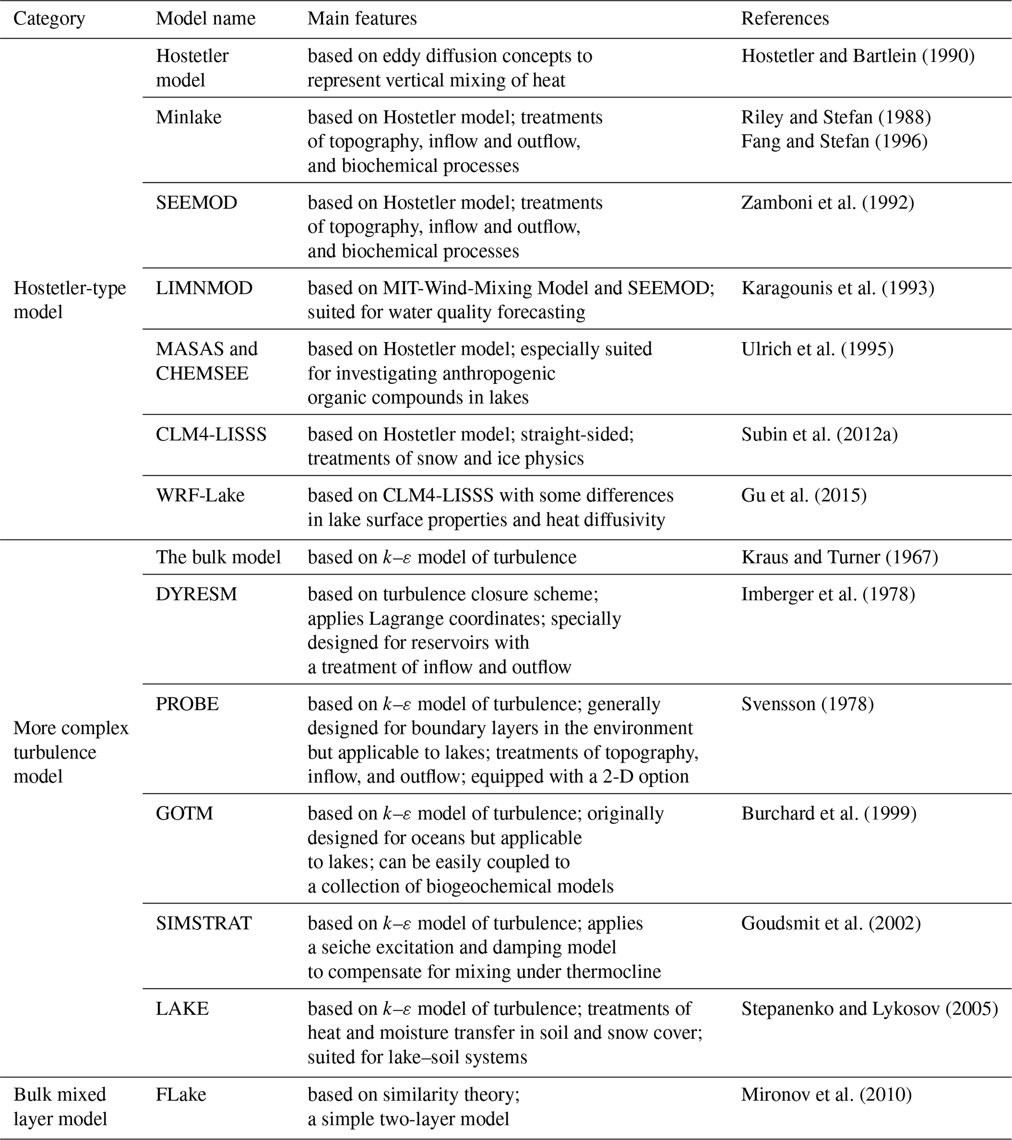
In contrast, one-dimensional (1-D) models have been widely used for coupling with atmospheric models, because 1-D models are sufficiently fast to facilitate long-term coupled simulations and have performed well in simulating seasonal and interannual variations of lake water temperature (Peeters et al., 2002). Depending on how they parameterize eddy diffusivity, these 1-D lake models mainly fall into two categories (MacKay et al., 2009; Perroud et al., 2009; Martynov et al., 2010; Stepanenko et al., 2010; Table 1): the Hostetler-type models, e.g., the Hostetler model (Hostetler and Bartlein, 1990; Hostetler et al., 1994), Minlake (Fang and Stefan, 1996), SEEMOD (Zamboni et al., 1992), LIMNMOD (Karagounis et al., 1993), MASAS and CHEMSEE (Ulrich, 1991), CLM4-LISSS (Subin et al., 2012a), and WRF-Lake (Gu et al., 2015); and the more sophisticated turbulence models, e.g., the bulk model of Kraus and Turner (1967), DYRESM (Imberger et al., 1978), PROBE (Svensson, 1978), GOTM (Burchard et al., 1999), SIMSTRAT (Goudsmit et al., 2002), and LAKE (Stepanenko and Lykosov, 2005; Stepanenko et al., 2011). The Hostetler-type models use parameterized eddy diffusivity to model vertical mixing in the lake body. The eddy diffusivity is dependent on surface wind speed and lake stratification and its parameterization follows that of Henderson-Sellers (1985), which is formulated under the assumptions of unstratified Ekman flow (Smith, 1979). Although the representativeness of this eddy diffusivity scheme for lakes has not been systematically evaluated, these models have been applied in numerous coupled simulations with regional climate models (Bates et al., 1995; Hostetler and Giorgi, 1995; Small et al., 1999) and general circulation models (Bonan, 1995; Krinner, 2003). The more complex turbulence models use the k–ε turbulence scheme and parameterize eddy diffusivity based on the Kolmogorov–Prandtl relation. Thus, the turbulence models require two additional equations for the turbulent kinetic energy (k) and its dissipation rate (ε). Although models from both categories have been intensively used in climate models, they share the potential and common drawback that the eddy diffusivity representations may be inappropriate when temperature gradients are weak (MacKay et al., 2009).

In addition to the above two categories, bulk mixed layer models have also been developed, including FLake (a relatively simple two-layer model based on the similarity theory; Mironov et al., 2010) as a typical example. Gula and Peltier (2012) and Mallard et al. (2014) have coupled FLake to WRF in one-way and two-way model configurations, respectively. However, it is difficult for these oversimplified lake models to capture seasonal stratification and to accurately simulate water temperature in deep lakes. Thus, the performance of the bulk mixed layer models in climate-modeling studies is still limited.

WRF-Lake is a 1-D lake model that has been widely applied to study how lakes affect local weather and regional climate (Gu et al., 2015, 2016; Mallard et al., 2015; Xiao et al., 2016). It is an eddy-diffusion model adapted from the Community Land Model (CLM) version 4.5 (Oleson et al., 2013) with further modifications by Gu et al. (2015). However, some previous studies and our evaluation here suggest that WRF-Lake is inaccurate when simulating deep lakes and reservoirs (Mallard et al., 2015; Xiao et al., 2016). To better represent thermodynamic processes of deep lakes and reservoirs in regional climate simulations, we here revised the WRF-Lake model. Our revisions fall into four categories: (1) including an improved spatial discretization scheme, (2) improving the surface property parameterization, (3) improving the diffusivity parameterization for deep lakes, and (4) improving the convection scheme to avoid unphysical mixing. We evaluated the improved lake model, WRF-rLake (i.e., revised lake model), at the Nuozhadu Reservoir, a deep reservoir (up to 200 m deep) in southwestern China, and conducted sensitivity experiments to evaluate the effect of dominant processes and parameters on simulated lake water temperature and surface heat fluxes.

Table 1Common 1-D lake models.

Download Print Version | Download XLSX

2 Model description and improvements

2.1 Description of the current WRF-Lake model

The WRF-Lake model is a mass and energy balance scheme which vertically divides the lake into 20–25 layers and solves the 1-D heat diffusion equation. The lake includes 0–5 snow layers, 10 lake liquid water and ice layers (hereafter lake body), and 10 sediment layers (Subin et al., 2012a). The lake body water content is assumed to be constant and sediment layers are fully saturated. An infinitely small interface is assumed between the first lake layer and the overlying atmosphere to calculate lake surface fluxes of heat, water mass, momentum, and radiation. After subtracting latent and sensible heat fluxes from the surface net all-wave radiation, the residual energy fluxes are set as the top boundary condition to force the heat diffusion equation. Mixing processes in the lake body include molecular diffusion, wind-driven eddy diffusion, and convective mixing (Hostetler and Bartlein, 1990). We describe below the basic model structure to indicate model processes and parameters that were analyzed and modified in this study.

2.1.1 Surface energy balance

In the WRF-Lake model, the energy balance at the lake surface is as follows:

\begin{matrix} (1) & S + L - G = H + λ E, \end{matrix}

where S is absorbed shortwave radiation, L is net longwave radiation, G is downward heat flux into the lake, H is sensible heat, and λE is latent heat. The units for all variables in Eq. (1) are watts per square meter (W m⁻²). In this equation, S is regulated by albedo (a); G, H, and λE are largely dependent on the thermal conductivity of the top lake layer (κ), aerodynamic resistance for heat (r_ah), and that for vapor (r_aw), respectively. A more thorough discussion of the relationship between lake surface fluxes and aerodynamic resistances is provided by Sect. 2.1.8 in Subin et al. (2012a).

2.1.2 Radiation transfer and absorption in the lake body

For unfrozen lakes, a fraction (β) of the incoming solar radiation is absorbed by the surface water within the first 0.6 m. The remaining solar radiation is absorbed by the lake body following Beer's law:

\begin{matrix} (2) & ϕ = (1 - a) (1 - β) S_{i} e^{- [η (z - z_{a})]}, \end{matrix}

where ϕ (W m⁻²) is the distribution of solar radiation with depth z (m; positive downward), β is set to a constant 0.4 (Oleson et al., 2010), z_a is the base of the surface absorption layer (0.6 m), and η is the light extinction coefficient (m⁻¹) which is calculated as a function of the lake depth according to Håkanson (1995):

\begin{matrix} (3) & η = 1.1925 d^{- 0.424}, \end{matrix}

where d (m) is the lake depth.

Though there exist more sophisticated radiation schemes in other lake models (e.g., the nine-band scheme by Paulson and Simpson, 1981), we kept the current WRF-Lake radiation scheme since it includes the essential components in a water-body physical radiation parameterization: an intensity-decaying formulation as a function of penetration depth following the Beer–Lambert law (Jerlov, 1976) and a scheme for absorption coefficients. Such an approach is also accepted by many other 1-D lake models (Fang and Stefan, 1996; Stepanenko and Lykosov, 2005). To improve the model performance, we tentatively set the cutoff depth z_a to be 0 m in this version as 0.6 m is usually an overestimated value, especially for shallow lakes (Deng et al., 2013). Although adopting this z_a value (0 m) demonstrates acceptable performance in this work, a more lake-specific cutoff depth may be needed for better model performance.

2.1.3 The heat diffusion solution

After the surface energy balance and radiation absorption are calculated, the following 1-D thermal diffusion equation is solved:

\begin{matrix} (4) & \frac{\partial T}{\partial t} = \frac{\partial}{\partial z} (k \frac{\partial T}{\partial z}) - \frac{1}{c_{w}} \frac{d ϕ}{d z}, \end{matrix}

where c_w is the volumetric heat capacity of water (J K⁻¹ m⁻³), T is water temperature (K), t is time (s), z is depth (m), k is the thermal diffusivity (m² s⁻¹), and ϕ is the solar radiation as in Eq. (3).

The thermal diffusivity k in WRF-Lake comprises molecular diffusivity (k_m) and wind-driven eddy diffusivity (k_e). k_m is a function of thermal conductivity and volumetric heat capacity of water ( $1.433 \times 10^{- 7}$ m² s⁻¹). k_e follows the Henderson-Sellers parameterization (shown in Appendix A) and is determined by wind speed at 2 m above the water surface, a latitude-dependent Ekman profile, and a lake-stratification-dependent Brunt–Väisälä frequency (Henderson-Sellers et al., 1983; Henderson-Sellers, 1985). However, for deep lakes, e.g., Lake Michigan (Martynov et al., 2010), Subin et al. (2012a) argued that increasing the eddy diffusivity by a factor of 10, and in some cases by a factor of 100, substantially improved simulated lake water temperatures and surface fluxes. Thus, in WRF-Lake, the eddy diffusivity for lakes deeper than 15 m was multiplied by a factor ranging from 10² to 10⁵ depending on lake depth and surface temperature (Gu et al., 2015).

2.1.4 Convective mixing

The convective mixing module is executed after the heat diffusion equation solution and is identical to that of Hostetler's lake model, which assumes that no temperature instability can be sustained in the lake body. In particular, at the end of any numerical time step, if there is denser water overlying lighter water, then convective mixing happens rapidly, mixing the lake body from surface to the unstable layers (Hostetler and Bartlein, 1990).

2.2 Improvements by WRF-rLake

As described below, we modified the existing WRF-Lake model (and named the revision WRF-rLake) by improving the spatial discretization scheme, parameterization for surface properties and vertical diffusivity, and convection scheme (Fig. 1).

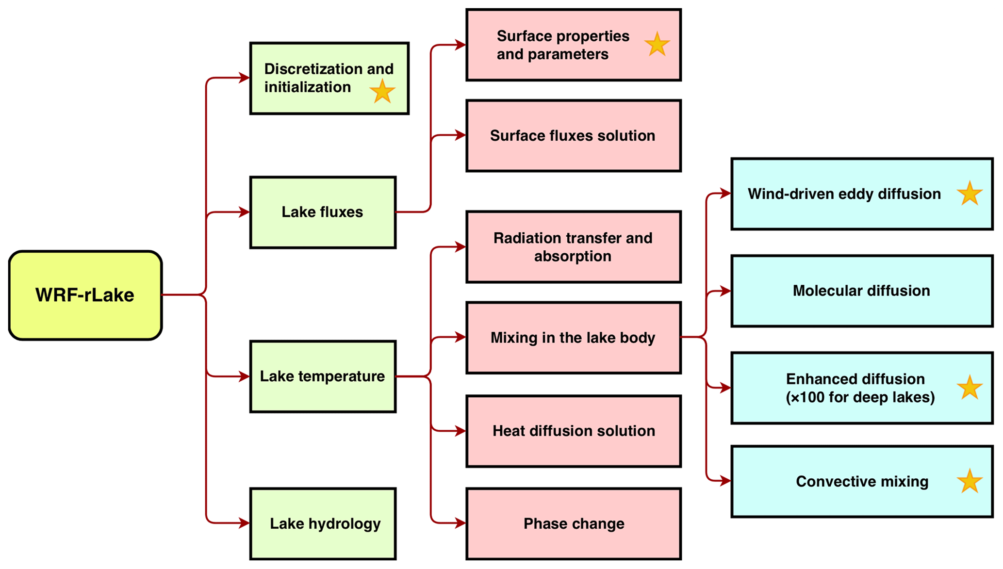
https://www.geosci-model-dev.net/12/2119/2019/gmd-12-2119-2019-f01

Figure 1Flow chart of the WRF-rLake model. The yellow star indicates the process is modified or newly added.

Download

2.2.1 Vertical discretization

The WRF-Lake model discretizes the water body into 10 layers, with the top-most layer fixed to 0.1 m (Gu et al., 2015) and each of the other nine layers constituting 10 % of the total depth. Although this discretization works well with shallow lakes (e.g., depth <50 m), it may be problematic for deep lakes in three aspects. The first is insufficient resolution. Discretizing lakes into only 10 layers is too coarse for the 200 m deep Nuozhadu Reservoir, resulting in only several layers to cover the thermocline. The second is depth loss, because the nine layers below the first layer only account for 90 % of the lake body, which, for very deep lakes, may cause up to approximately 10 % lake depth loss and will potentially lead to energy loss of the simulated lake system. The third is the large layer thickness transition between the first two layers. In the case of the Nuozhadu Reservoir (∼200 m deep), the default discretization results in a sharp thickness increase from 0.1 to 20 m (200 times) between the top two layers, which may be numerically problematic.

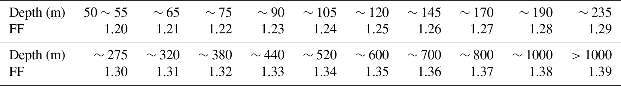
We therefore introduced a new discretization scheme for the lake body where both the vertical resolution and layer depth distribution are improved. For lakes deeper than 50 m, a 25-layer discretization scheme is used where the topmost layer is set to 0.1 m and the remaining layers have their thicknesses increasing exponentially by a fixed factor (FF) that depends on lake depth (Table 2). For the Nuozhadu Reservoir, FF is taken to be 1.29, which results in a series of layer depths (m) from the top to the bottom of 0.1, 0.1, 0.2, 0.2, 0.3, 0.4, 0.5, 0.6, 0.8, 1.0, 1.3, 1.6, 2.1, 2.7, 3.5, 4.6, 5.9, 7.6, 9.8, 12.6, 16.3, 21.0, 27.1, 35.0, and 44.7 m. Similar discretization techniques are widely used by various geoscientific models to improve model performance, e.g., the grid stretching in GFDL HiRAM (Harris et al., 2016) and nonuniform meshing in MPAS (Skamarock et al., 2018) etc. When a lake is less than 50 m deep, a new 10-layer discretization scheme is applied where the top layer is fixed at 0.1 m and the remaining depth is allocated evenly among the remaining nine layers.

Table 2Fixed factors (FFs) for vertical discretization for different lakes based on depth.

Download Print Version | Download XLSX

2.2.2 Surface properties and parameters

As discussed in Sect. 2.1.1, the aerodynamic resistances for heat (r_ah) and vapor (r_aw) heat fluxes are critical for surface energy balance predictions. The aerodynamic resistances are functions of momentum (z_0 m) and scalar roughness lengths (z_0 h for sensible heat and z_0 q for latent heat). In WRF-Lake, z_0 m is set to 1, 5, and 2.5 mm for unfrozen lakes, frozen lakes without snow, and frozen lakes with snow, respectively; while z_0 h and z_0 q are always kept equal to z_0 m.

However, for unfrozen lakes, the momentum roughness length of 1 mm is often too large. Open seas are believed to have larger roughness lengths than lakes due to better developed surface moving waves, while the Engineering Sciences Data Unit (ESDU) (1972) documentation suggested z_0 m=1 mm for normal and 0.1 mm for calm seas. A number of lake studies also have shown 1 mm to be a maximum z_0 m value. For example, measurements on Lake Washington in the US show z_0 m is generally below 1 mm and ranged between 0.01 and 1 mm (Atakturk and Katsaros, 1999); measurements on Lake Ngoring, a high-altitude lake in the Tibetan Plateau, found z_0 m ranged between 0.001 and 1 mm and seldom went beyond 1 mm (Li et al., 2015). Thus, in order to produce more realistic roughness lengths for lakes, CLM4-LISSS parameterized z_0 m based on the forcing wind, friction velocity, fetch, and lake depth. Adopting these parameterizations has produced more accurate surface heat fluxes and lake surface temperatures (LSTs) over many natural lakes (Subin et al., 2012a).

We therefore adopted the CLM4-LISSS parameterization of roughness lengths with some further modifications:

z_0 m is set to 2.4 mm for frozen lakes with snow and 1 mm for frozen lakes without explicit snow layers, and z_0 h and z_0 q are computed as functions of z_0 m and friction velocity u_* (m s⁻¹).
For unfrozen lakes, z_0 m is parameterized as follows:
$\begin{matrix} (5) & z_{0 m} = max (\frac{γ ν}{u_{*}}, α \frac{u_{*}}{g}), \end{matrix}$
where γ is a dimensionless empirical constant (0.1), α is the dimensionless Charnock coefficient described below, and g is the acceleration of gravity (Fairall et al., 1996; Charnock, 1955; Smith, 1988):
$\begin{array}{l} (6) & α = α_{min} + (α_{max} - α_{min}) \exp [- min (A, B)], \\ (7) & A = {(\frac{F g}{u^{2}})}^{1 / 3} /f_{c}, \\ (8) & B = ε \frac{\sqrt{d g}}{u}, \end{array}$
where F (m) is the lake fetch (assumed to be 25 times the lake depth when observations are unavailable), u (m s⁻¹) is 2 m wind speed, d (m) is lake depth, $α_{min} = 0.01$ , $α_{max} = 0.11$ , and ε=1. A and B account for influences from fetch and depth, respectively.

We also made further improvements in roughness length parameterizations for unfrozen lakes. In LISSS, f_c should be 100 but was tentatively set to 22, corresponding to the use of u instead of u_* in Eq. (7). Subin et al. (2012a) recommended that future lake models should relax this assumption by setting f_c=100 and directly applying u_* rather than u, which we have done in WRF-rLake. Because u_* depends on surface roughness lengths, which in turn depend on u_*, we introduced a fixed-point iteration for the equations relating u_* and surface roughness lengths. It is worth noting that the parameterization of roughness lengths for frozen lakes could also be improved. However, as the Nuozhadu Reservoir is unfrozen throughout the year, we did not make any modifications to the representations for lake ice. Future work should investigate lakes with frozen periods to further improve the roughness length parameterization.

2.2.3 Improved diffusivity parameterization

The Henderson-Sellers parameterization (see Appendix A) for wind-driven eddy diffusivity underestimates mixing in deep lakes and was therefore increased in WRF-Lake by a multiplicative factor (Gu et al., 2015). However, this treatment may trigger new problems. As k_e declines exponentially with depth (Eq. A1), it is more likely to be underestimated in deeper layers than in the topmost one. Thus, enlarging k_e by the same factor for the whole lake may introduce new problems in two ways.

First, k_e may be overestimated in lake surface layers. A number of empirical studies have estimated the effective vertical heat diffusivity in lakes and coastal oceans using heat flux measurements and tracer distribution measurements. These studies showed that vertical heat diffusivity in natural lakes seldom exceeds ∼1 cm² s⁻¹ and in oceans, where the forcing winds are usually stronger and moving surface waves are better developed, vertical heat diffusivity exceeds ∼10² cm² s⁻¹ (Hutchinson, 1957; Li, 1973; Kullenberg et al., 1973; Kullenberg, 1974; Jassby and Powell, 1975; Sarmiento et al., 1976; Quay et al., 1980). We thus set a maximum of 10² cm² s⁻¹ for wind-driven eddy diffusivity (corresponding to the maximum value for open seas) to avoid overestimation in surface layers.

Second, for deep layers, k_e may still be underestimated by WRF-Lake because k_e is forced to decline exponentially with depth. Additional diffusion terms should be included to account for turbulent mixing generated by other mechanisms in deeper layers where wind-driven eddies cannot penetrate. So, in WRF-rLake, we adopted the enhanced diffusion term, D_ed (m² s⁻¹), from CLM4-LISSS (Ellis et al., 1991; Fang and Stefan, 1996; Subin et al., 2012a), which was originally suggested by Hondzo and Stefan (1993) to compensate for unresolved turbulence (even below ice or at large depth) and is given as follows:

\begin{matrix} (9) & D_{ed} = δ {(N^{2})}^{- 0.43}, \end{matrix}

where δ is the level of turbulence which can be related to lake area, and N (s⁻¹) is the Brunt–Väisälä frequency (a minimum N² is suggested to be $7.5 \times 10^{- 5}$ s⁻²). CLM4-LISSS adopted the values measured at an ice-covered lake (Fang and Stefan, 1996) for Eq. (9) by setting $δ = 1.04 \times 10^{- 8}$ . However, as discussed by Subin et al. (2012a), this suggested value for D_ed is only several times larger than k_m and may still be too small for deep lakes. Therefore, for lakes deeper than 50 m, we imposed an increase in δ by a factor of 100 for all layers but admit that this coefficient may vary from lake to lake (partially explained by lake area) and thus needs to be tuned under specific scenarios.

2.2.4 Convective mixing

In WRF-Lake, density instability is the prerequisite for convective mixing. As we have mentioned above, density for each water layer is first calculated based on lake water temperature, then adjacent layers are compared for their densities to determine whether there should be convective mixing. However, since the water density is calculated as a function of temperature, when the temperature gradient between two adjacent layers is small (usually less than 10⁻³ K m⁻¹, but still with a lighter layer overlying a heavier layer), small numerical errors may incorrectly trigger convective mixing. In WRF-rLake we therefore set a density gradient threshold of 10⁻⁴ kg m⁻³ m⁻¹ (which is equivalent to a temperature gradient threshold of about 10⁻³ K m⁻¹) to avoid this unphysical convective mixing. In our tests at Nuozhadu Reservoir, convective mixing can penetrate as deep as 5 m below the surface in WRF-Lake, while it is almost always restricted within the top 1 m in WRF-rLake.

3 Data and modeling experiments

3.1 Study area

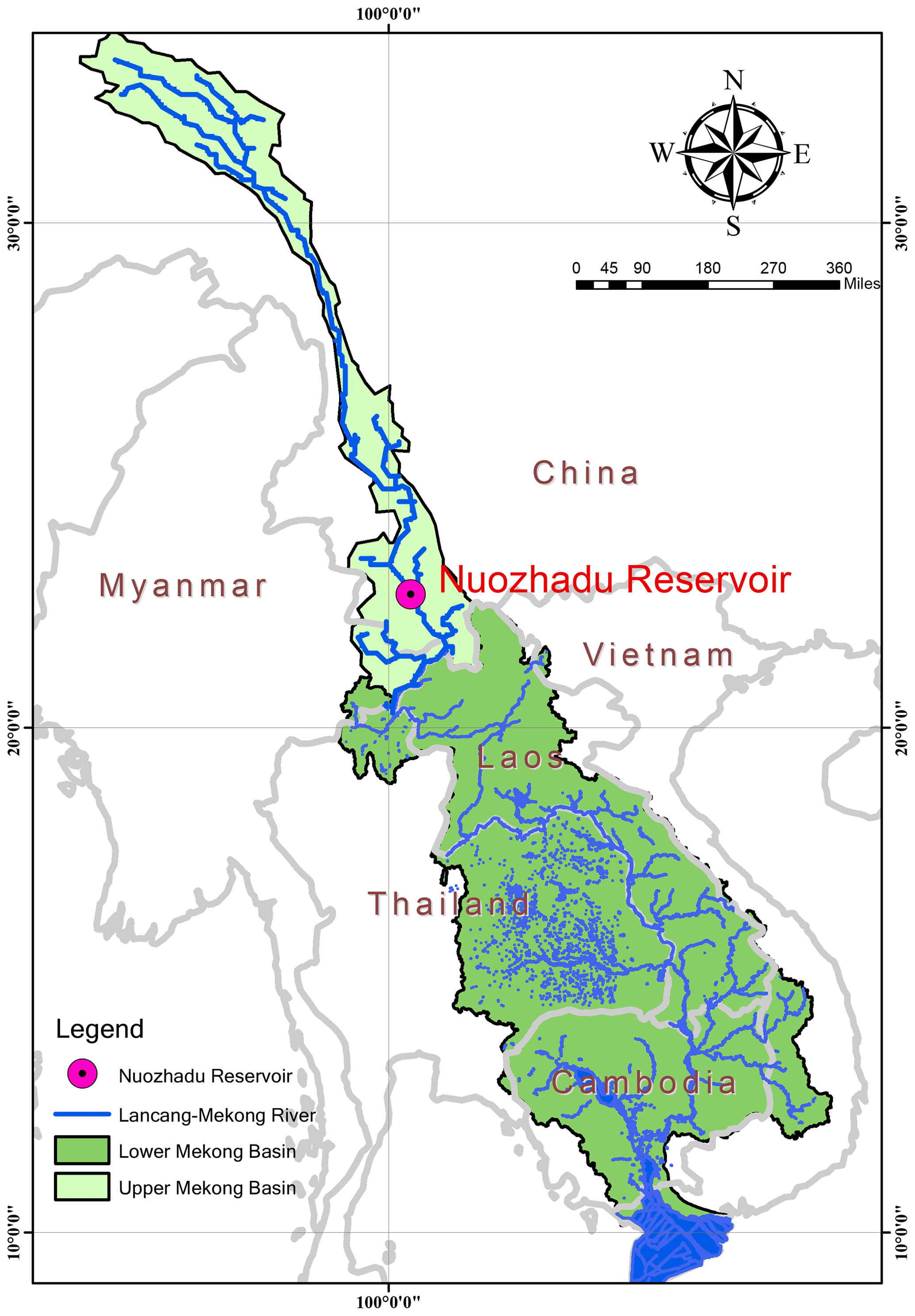
The Nuozhadu Reservoir is near the downstream end of a group of reservoirs along the Lancang River (22^∘38^′ N, 100^∘26^′ E), which is located in southwestern China and is called the Mekong River when it leaves China and enters Laos (Fig. 2). The Nuozhadu Reservoir has a dam height of 262 m and a normal water level¹ of 812 m a.s.l. The water depth upstream of the dam in the year 2015 is around 200 m. The water surface area has increased more than 10 times after construction of the reservoir. Owing to its particular location, great depth, and large surface area, the Nuozhadu Reservoir serves as a good example for research on the impacts of artificial inland waters on regional climate.

https://www.geosci-model-dev.net/12/2119/2019/gmd-12-2119-2019-f02

Figure 2Location of the Nuozhadu Reservoir.

Download

3.2 Forcing data

Our study period covers from 1 January to 31 December 2015, a year when the reservoir was under normal operation. We ran the lake module off-line, driven directly by forcing data acquired from local meteorological stations rather than WRF-simulated fields, in order to evaluate the lake module free from potential biases originating in WRF. The forcing data of the first day were repeated 7 times to form a 1-week spinup. The downward shortwave radiation and downward longwave radiation were obtained from the China Meteorological Forcing Dataset (Kun et al., 2010; Chen et al., 2011), which has a temporal resolution of 3 h and spatial resolution of $0.1^{\circ} \times 0.1^{\circ}$ . A linear interpolation was applied to these data to obtain hourly forcing for WRF-rLake. Although it probably underestimates peak radiation values, linear interpolation may still be considered to be an acceptable approximation given no data of higher temporal resolution are available.

Other forcing data, including atmospheric temperature, atmospheric pressure, atmospheric specific humidity, atmospheric wind speed in the east and north directions, and precipitation, were acquired with a 1 h temporal resolution from a meteorological observatory run by China Huaneng Group Co., Ltd., the construction unit of the Nuozhadu Reservoir (Fig. 3). The station (22^∘40^′ N, 100^∘23^′ E) is located about 5 km upstream (or northwest) of the Nuozhadu Dam and has an observational height of 10 m.

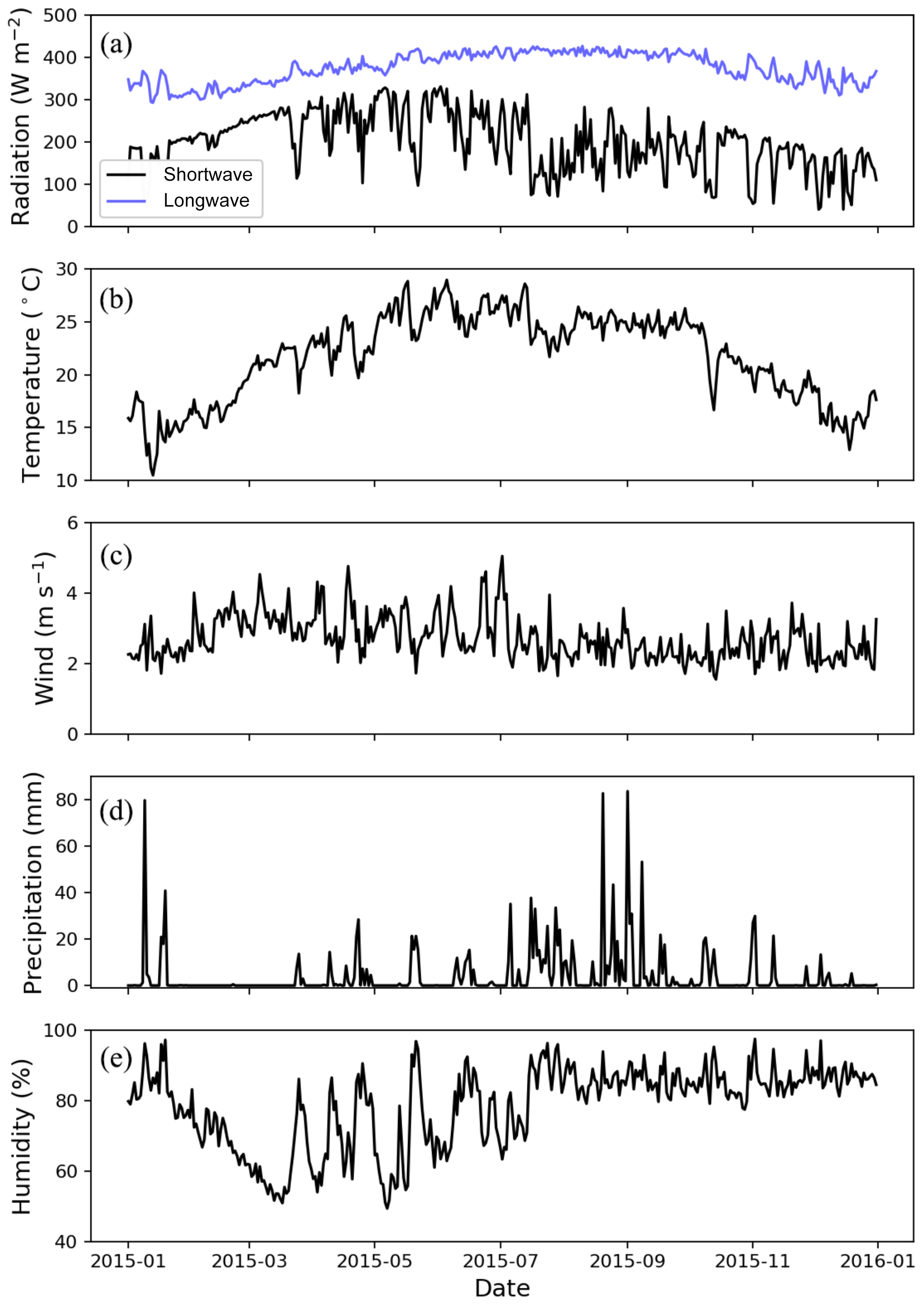
https://www.geosci-model-dev.net/12/2119/2019/gmd-12-2119-2019-f03

Figure 3The year-long meteorological forcing data used include (a) shortwave and longwave radiation, (b) air temperature, (c) wind speed, (d) precipitation, and (e) humidity. All data are averaged to produce mean daily values.

Download

3.3 Observations for model initialization and evaluation

Water temperature was measured hourly from 712 m to 804 m a.s.l. at an interval of 2 m near the Nuozhadu dam during 2015 (Fig. 4). Since the reservoir is in a tropical region, surface water temperature is higher than 20^∘ throughout the year. In 2015, the water level was dropped from January to June in preparation for the rainy season and rose gradually thereafter from July to December.

Measured water temperature on 1 January 2015 was used to initialize the first 90 m of the water body. The remaining 110 m of depth (for which observations were not made) were initialized using simulated results at the same site on the same day by Delft3D FLOW (Shen, 2017), a three-dimensional hydrodynamic model proven to be sufficiently accurate at the Nuozhadu Reservoir.

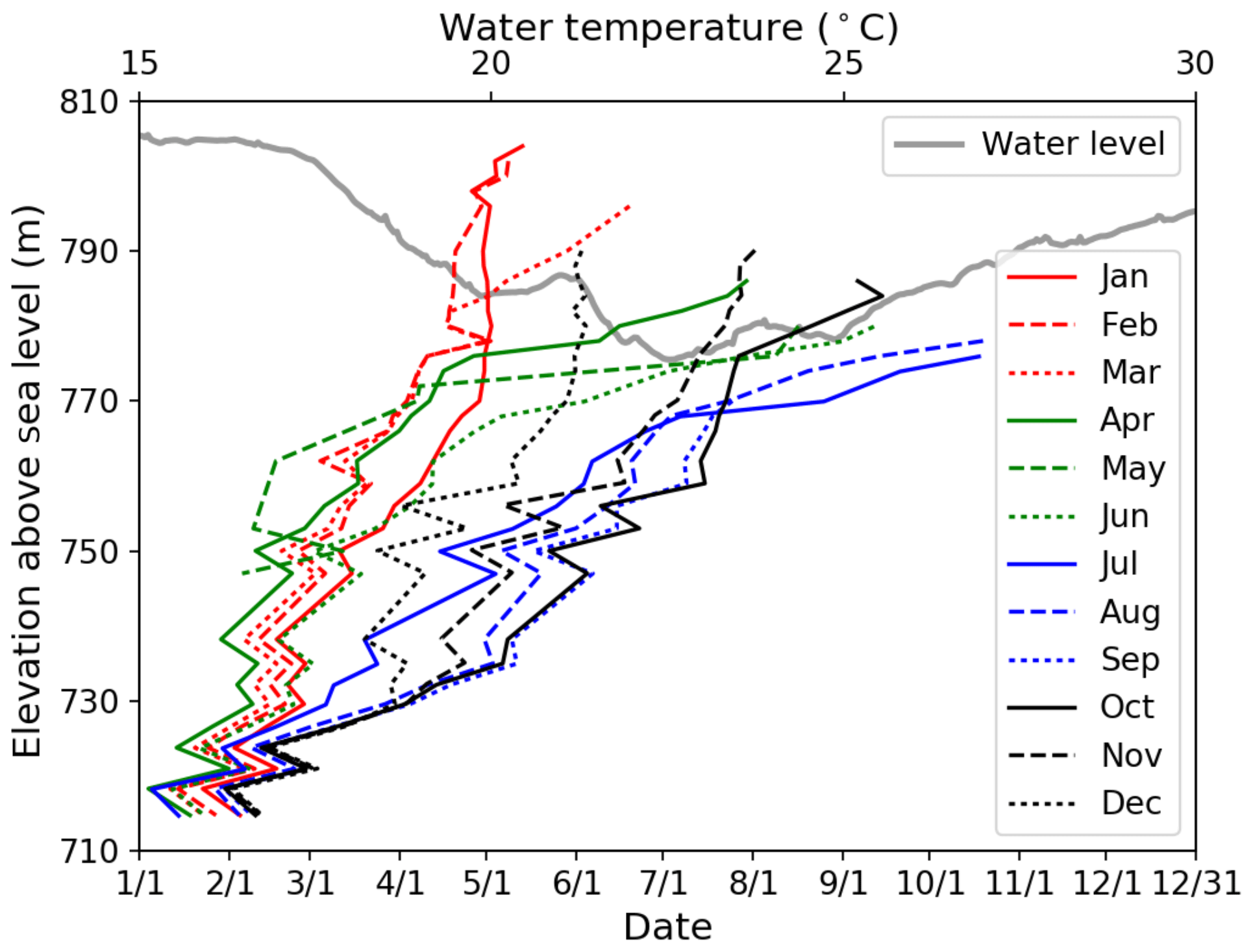
https://www.geosci-model-dev.net/12/2119/2019/gmd-12-2119-2019-f04

Figure 4Measured monthly water temperature profile for Nuozhadu Reservoir in the year 2015. The light gray line indicates the water level variation throughout the year.

Download

3.4 Numerical experiments

To examine the incremental improvements in the WRF-rLake simulations, we performed four sets of off-line numerical experiments analyzing four key parameterizations (Table 3):

Vertical discretization (“Lyr” set). the default WRF-Lake 10-layer and modified 25-layer settings were contrasted to assess the impacts of different vertical discretization schemes.
Vertical Diffusivity (“Diff” set). we examined the impact of vertical diffusivity by applying different diffusivity schemes: the original scheme by Hostetler and Bartlein (1990), the scheme by Gu et al. (2015), the scheme by Gu et al. (2015) with enhanced diffusion terms, and the scheme as discussed in Sect. 2.2.3 or called “modified” diffusivity as adopted by our new model WRF-rLake.
Roughness length (“Rou” set). momentum and scalar roughness lengths are set to 1, 10 mm, calculated as in Subin et al. (2012a), or calculated with further modification as in Sect. 2.2.2, to examine the effects of different roughness lengths schemes.
Light extinction coefficient (“Ext” set). through model tests, we conclude that in addition to the schemes we modified, the light extinction coefficient is also a key parameter for accurately modeling deep lakes (Hocking and Straškraba, 2015). Although the default parameterization of light extinction coefficient has been applied in previous WRF-Lake studies (e.g., Gu et al., 2015), we tested the impacts of different values of this coefficient. Given that no Secchi disk measurements were available in our study site, no empirical constrains for the light extinction coefficient could be directly developed. Thus, we tested a range of light extinction coefficient values: 0.13 m⁻¹ (default), 0.30, 1.00, and 3.00 m⁻¹. Although measurements have reported larger variability in the light extinction coefficient (e.g., 0.05 to 7.1 m⁻¹ in Subin et al., 2012a), we found simulated temperature profiles were insensitive to values outside of the 0.13 to 3.0 m⁻¹ range. We concluded that the best performance could be achieved by increasing the light extinction coefficient to ∼1.00 m⁻¹, which thus is adopted in our baseline run (BL).

In addition, a control run (CTL) was configured with default roughness lengths, extinction coefficient, and vertical diffusivity (Gu et al., 2015) as in the default WRF-Lake, and a baseline run (i.e., our proposed new model structure) was configured with all modifications described in Sect. 2.2 and a tuned light extinction coefficient to demonstrate the effects of each improvement in WRF-rLake.

Table 3An overview of numerical experiments designed to demonstrate sensitivity in WRF-rLake.

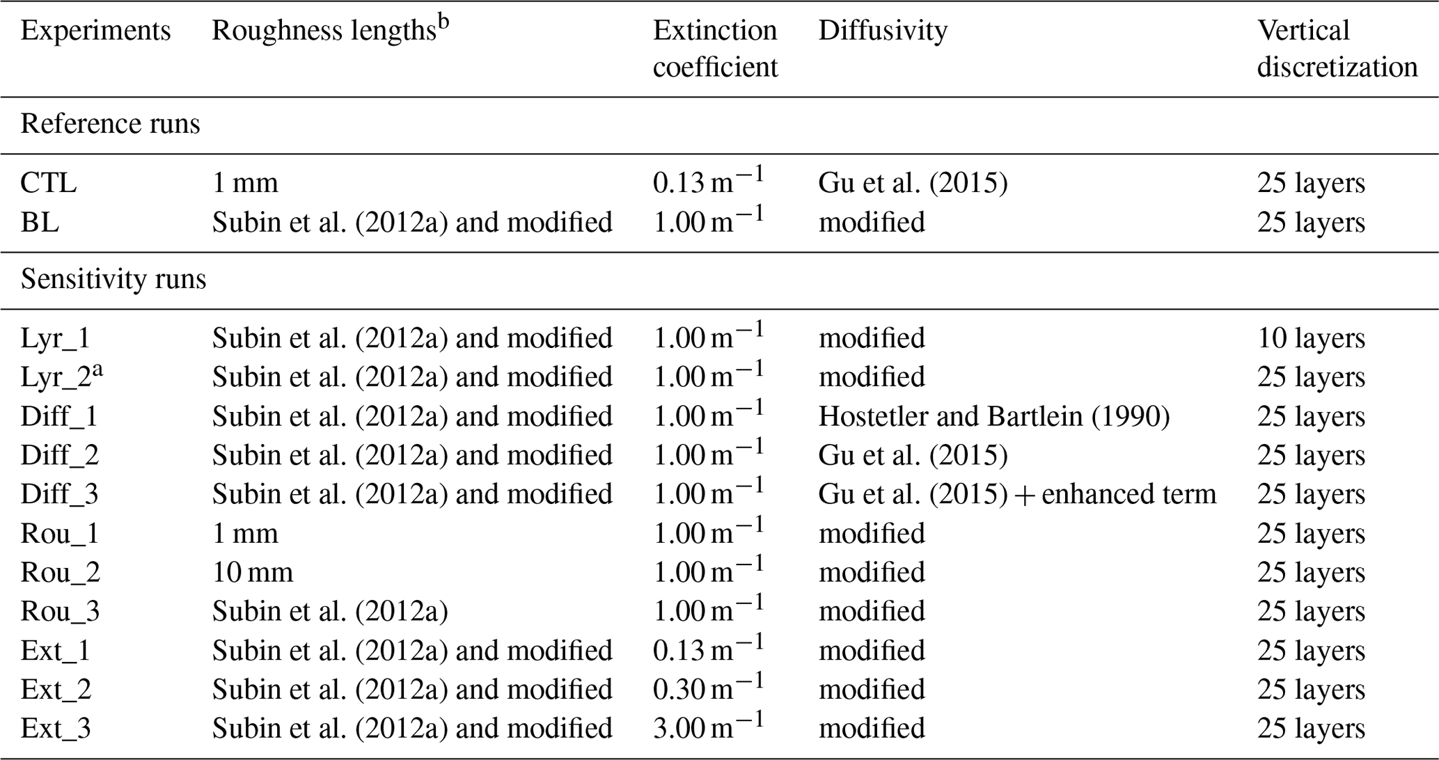
^a Configuration of Lyr_2 is the same as BL.
^b As the reservoir was ice-free in the year 2015, the constants given in this column refer to the roughness lengths for unfrozen lakes.

Download Print Version | Download XLSX

4 Results and discussion

4.1 Comparison of simulated temperature fields between WRF-Lake and WRF-rLake

The simulation results near the dam, the same place where the observations were collected, were used to conduct the evaluation. In comparing WRF-Lake simulations (CTL) to the observations (Fig. 5), the LSTs are underestimated most of the time with a mean bias error (MBE) of −0.69 ^∘C. The largest bias is found in the first quarter where it reached −3.37 ^∘C. This bias mainly resulted from the overestimation of roughness lengths by prescribing them to 1 mm, which resulted in overly large outgoing latent and sensible heat fluxes (Sect. 4.2).

https://www.geosci-model-dev.net/12/2119/2019/gmd-12-2119-2019-f05

Figure 5Time series of lake surface temperatures by observation (red dots), baseline (BL: black line), control (CTL: blue line), Diff_3 (green line), and air temperature (gray dashed line) of Nuozhadu Reservoir for the period 1 January 2015 through 31 December 2015.

Download

The configuration Diff_3 (with “half” modified diffusivity) overestimated LSTs by up to 5.55 ^∘C, reaching an MBE of 0.61 ^∘C. Seasonally, the LSTs are very well reproduced in the first and fourth quarter but are overestimated in the second and third quarter of the year. The vertical temperature profile (Fig. 6) shows that in the second and third quarters, Diff_3 simulated too much vertical mixing in the top 10 m, resulting in warmer water temperatures in this zone. Meanwhile, a sharp temperature decline is observed between 10 and 20 m depth followed by an underestimation of temperature below 20 m, suggesting overly weak vertical mixing simulated below 20 m. Further discussion in terms of diffusivity is shown in Sect. 4.3. Here the results of other diffusivity experiments (i.e., Diff_1 and Diff_2) are not shown.

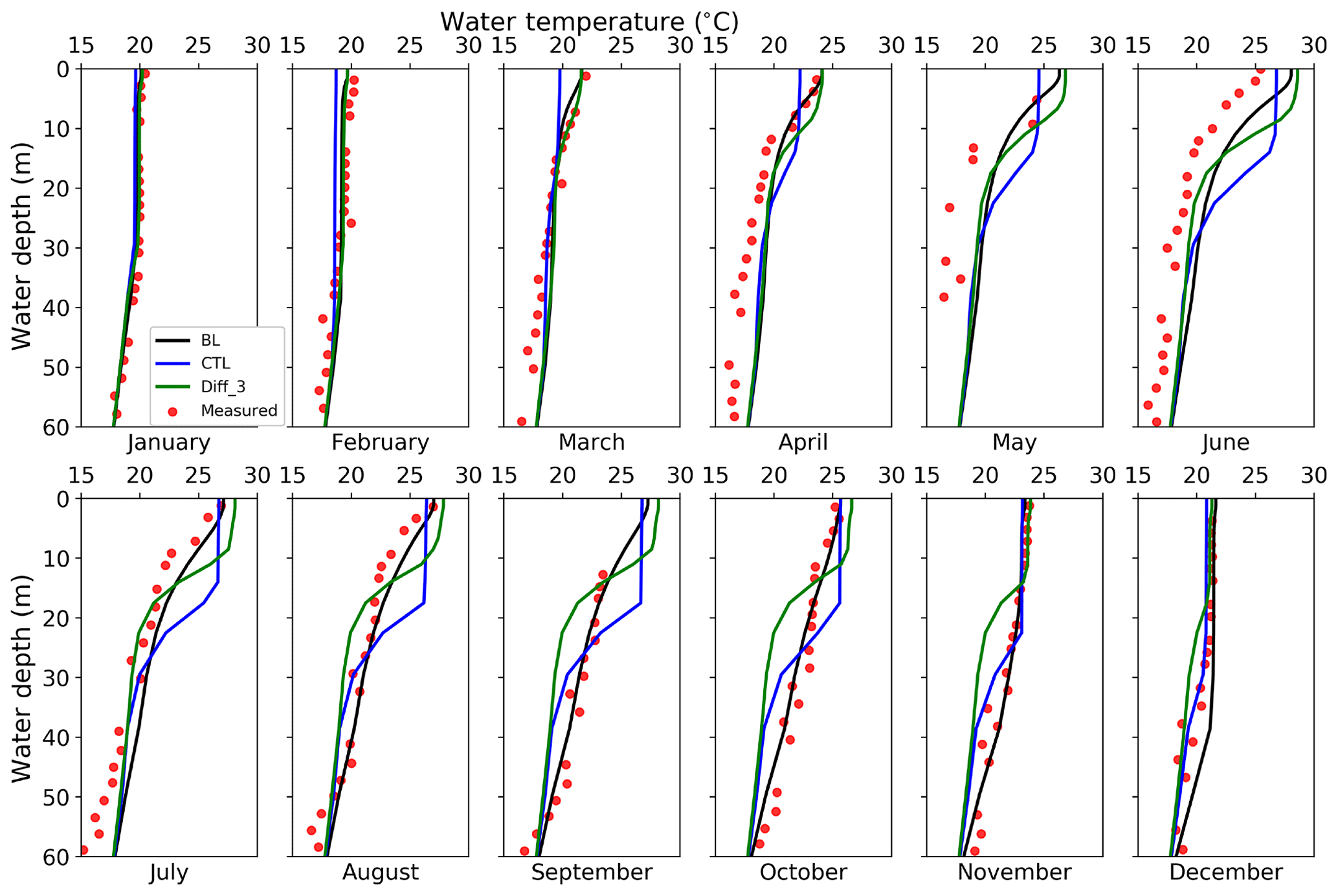
https://www.geosci-model-dev.net/12/2119/2019/gmd-12-2119-2019-f06

Figure 6Monthly vertical temperature profiles for the first 60 m water in the year 2015 by observation (red dots), BL (black line), CTL (blue line), and Diff_3 (green line).

Download

The simulation by BL is better in terms of root-mean-square error (RMSE) of simulated LSTs, which is reduced to 1.14 ^∘C from 1.35 ^∘C by CTL. Vertical temperature profiles were also improved, as the thermocline in the top 10 m is reproduced in hot seasons, in contrast to the CTL and Diff_3 simulations. More detailed statistical metrics of the vertical temperature profile (Table 4) suggest that BL gives the best simulations among the three simulations compared.

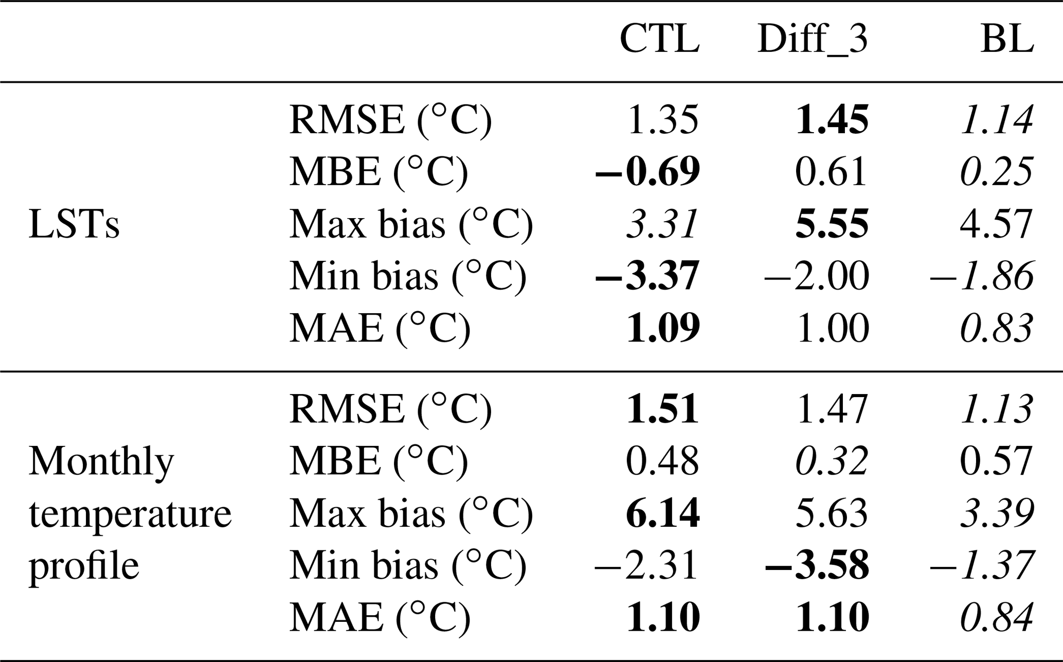
Table 4Statistics of the discrepancy between simulated (CTL, Diff_3, and BL) and observed LSTs and monthly temperature profiles during year 2015. Root-mean-square error (RMSE) and Mean Absolute Error (MAE) are calculated between each simulation and measurement. Mean bias error (MBE), max bias, and min bias are computed by simulation minus measurement. Bold and italic font indicate the largest and smallest absolute values among three simulations, respectively.

Download Print Version | Download XLSX

Applying all the modifications to vertical diffusivity (discussed in Sect. 2.2.4), we obtained the best simulations by BL; however, we note that the original diffusivity parameterization of Henderson-Sellers (1985) may be inappropriate for deep lakes as this parameterization finds it hard to yield good diffusivity simulations for deep lakes without tuning. Thus, we suggest more thorough evaluation and modification to this parameterization should be carried out in future research.

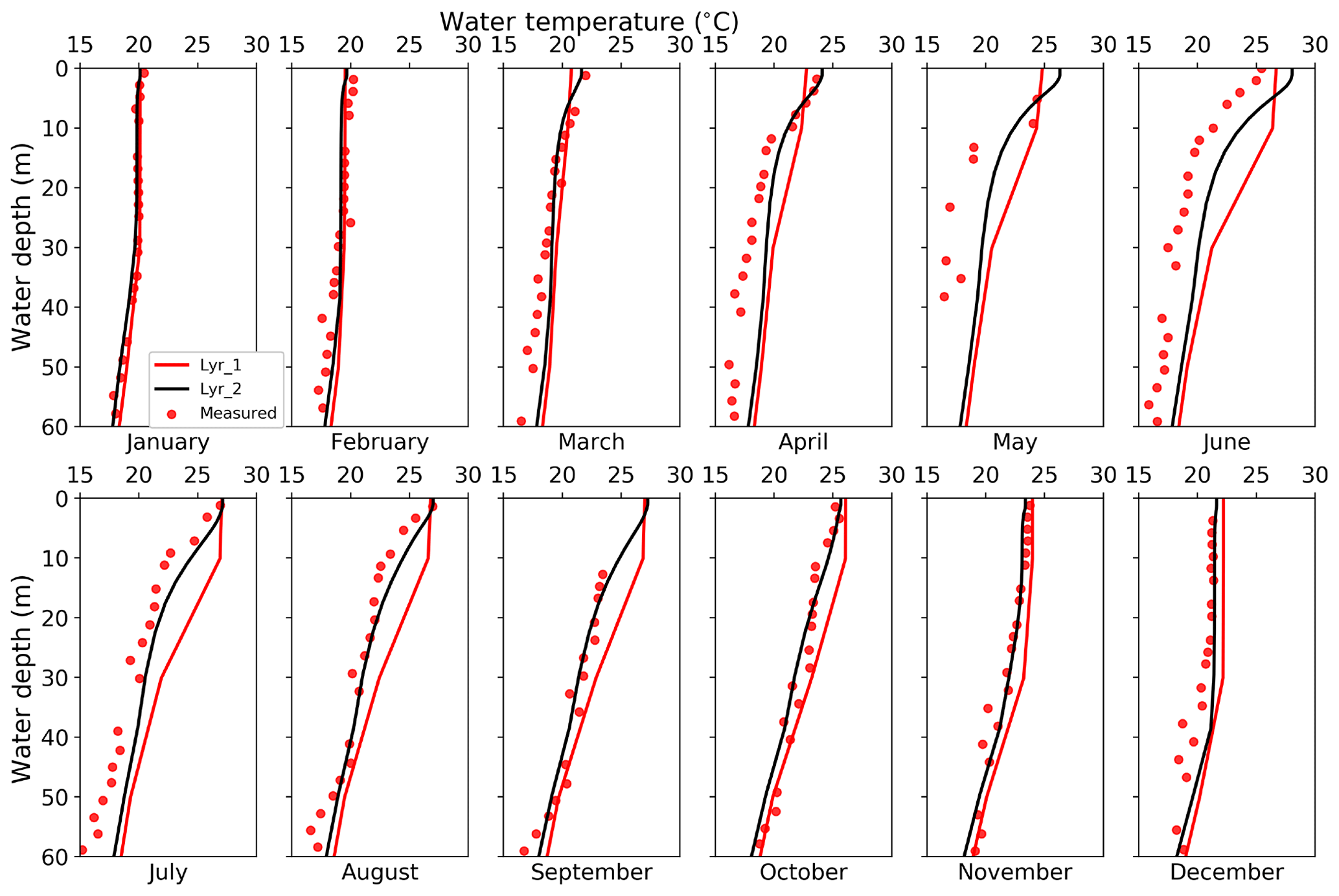
https://www.geosci-model-dev.net/12/2119/2019/gmd-12-2119-2019-f07

Figure 7Monthly vertical temperature profile for the first 60 m water by observation (red dots), Lyr_1 (red line), and Lyr_2 (black line) in the year 2015.

Download

4.2 Effects of vertical discretization

In these experiments, Lyr_1 adopted the default WRF-Lake 10-layer scheme and was identical to BL except for discretization. Lyr_2 (identical to BL) uses the modified 25-layer scheme. Overall, compared to Lyr_1, Lyr_2 reduced the RMSE against monthly observed lake temperatures profiles from 1.64 to 1.13 ^∘C. Lyr_1 predicted too much vertical mixing in the top 10 m, failing to reproduce the thermocline in this zone in summer (Fig. 7). In the first 2 months, the temperature difference in the top 10 m between Lyr_2 and Lyr_1 was not obvious. But as the lake warms up, the thermocline in Lyr_2 (top 10 m) is intensified, hindering heat transfer to the underlying layers, which in turn further strengthened the thermocline. However, this process is not captured by the Lyr_1 model; rather, a well-mixed water column in the top 10 m (top two layers) is simulated throughout the year. From March to June, the overmixing by Lyr_1 also resulted in colder LSTs, which in turn produced lower sensible and latent heat fluxes by up to 10 and 20 W m⁻², respectively (not shown). Lower outgoing heat fluxes kept more energy stored in the lake body, explaining why the whole lake body became increasingly warmer throughout the summer compared to Lyr_2. This underestimation of outgoing heat fluxes was reversed when the surface temperature in Lyr_1 finally exceeded that of Lyr_2 and produced more sensible and latent heat fluxes to the atmosphere from October to December.

In summary, the 10-layer scheme produced more uniform temperature fields across the water column and, due to its coarser spatial discretization, poorly predicted the thermocline where temperature changes rapidly. We further tested a 100-layer scheme but its simulations did not differ significantly from the 25-layer scheme (not shown here), so we conclude that the 25-layer scheme is sufficient for deep lakes like the Nuozhadu Reservoir.

4.3 Effects of diffusivity

BL, Diff_1, Diff_2, and Diff_3 form a group of sensitivity experiments for diffusivity. In the case of the Nuozhadu Reservoir, Diff_2 applies the eddy diffusivity of Diff_1 with an increase of 100 times throughout all layers, as in Gu et al. (2015); Diff_3 additionally includes the enhanced diffusion term on top of Diff_2.

For the monthly-averaged vertical temperature profile (Fig. 8), the BL scheme best captures the decrease in water temperature with depth and LSTs. BL yields the smallest RMSE of 1.13 ^∘C against monthly observed lake temperatures profiles, while Diff_1, Diff_2, and Diff_3 yield 1.62, 1.47, and 1.47 ^∘C, respectively. Diff_1 yields strong stratification within 10 m of the surface, indicating that the eddy diffusivity by Hostetler and Bartlein (1990) is too small and prevents heat from transferring from the surface to depth. This suppression reduces heat stored in the lake body and weakens the thermal inertia of the lake, leading to LSTs that are biased high in summer and LSTs that are biased low in winter.

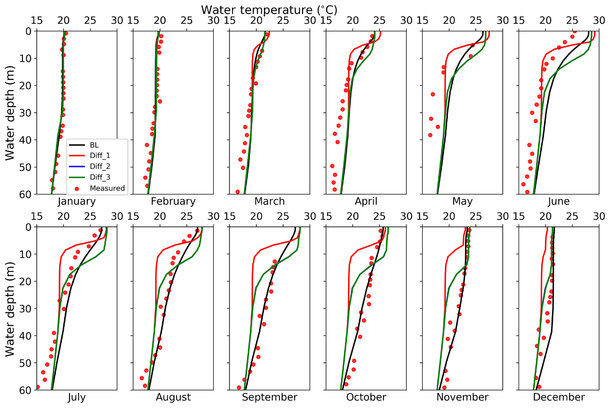
https://www.geosci-model-dev.net/12/2119/2019/gmd-12-2119-2019-f08

Figure 8Monthly vertical temperature profiles for the first 60 m water by observation (red dots), BL (black line), Diff_1 (red line), Diff_2 (blue line), and Diff_3 (green line) in the year 2015. Note Diff_2 and Diff_3 overlap each other.

Download

Diff_2 and Diff_3 produce identical vertical temperature profiles, indicating that the enhanced diffusion term is relatively small compared to eddy diffusivity and makes little difference. Diff_2 and Diff_3 produce lake layers of almost uniform temperatures in the top 10 m (Fig. 8). This pattern is further confirmed by the strong vertical mixing in the first 10 m inferred by the vertical profile of overall diffusivity that includes molecular, eddy, and enhanced diffusivity (Fig. 9). The overall diffusivity by Diff_2 in the top 10 m could be as large as 10³ cm² s⁻¹, which is too large compared to estimates in the literature (Sect. 2.2.3), supporting the necessity for limiting eddy diffusivity (Sect. 2.2.4).

https://www.geosci-model-dev.net/12/2119/2019/gmd-12-2119-2019-f09

Figure 9Monthly vertical diffusivity profile for the first 60 m water by BL (black line), Diff_1 (red line), Diff_2 (blue line), and Diff_3 (green line) in the year 2015. The gray shading indicates the diffusivity range of Lake Zürich reported by Li (1973).

Download

The overall vertical diffusivity below 20 m by Diff_2 or Diff_3 is of the same magnitude as molecular diffusivity ( $1.43 \times 10^{- 3}$ cm² s⁻¹). By increasing the enhanced diffusion term by 100 times for deep lakes, BL yielded more reasonable vertical diffusivity below 20 m (Fig. 9), which is quite close to an estimation at a very similar lake: Li (1973) estimated the vertical diffusivity in Lake Zürich, a lake with similar topography and depth (∼130 m deep) to the Nuozhadu Reservoir, and concluded its value for vertical diffusivity mostly ranged between 0.1 and 1 cm² s⁻¹.

With the constrained eddy diffusivity and “enhanced diffusion term”, BL produced the best temperature profiles compared to observations (Fig. 8). Further, the total diffusivity affects both the shape of vertical temperature profiles and the quantity of energy transferred down from the surface, which further influences LSTs.

4.4 Effects of roughness lengths

We next compare BL, Rou_1, Rou_2, and Rou_3, experiments that were conducted with different roughness length parameterizations, where the latter three have roughness lengths of 1, 10 mm, and the parameterization from the Subin et al. (2012a) scheme. In BL, the value of roughness values varied but were almost always smaller than Rou_1 and Rou_2 (generally less than 0.5 mm). BL and Rou_3 produced almost identical LSTs (Fig. 10) and latent and sensible heat fluxes (Fig. 11), suggesting that the modification added in Sect. 2.2.2 (i.e., setting f_c equal to 100 and applying u_* rather than u in Eq. 7), although being more realistic, do not influence the overall performance of WRF-rLake significantly. BL performs better in terms of RMSE of simulated LSTs, which is 1.14 ^∘C compared to 1.34 ^∘C by Rou_1 and 2.46 ^∘C by Rou_2.

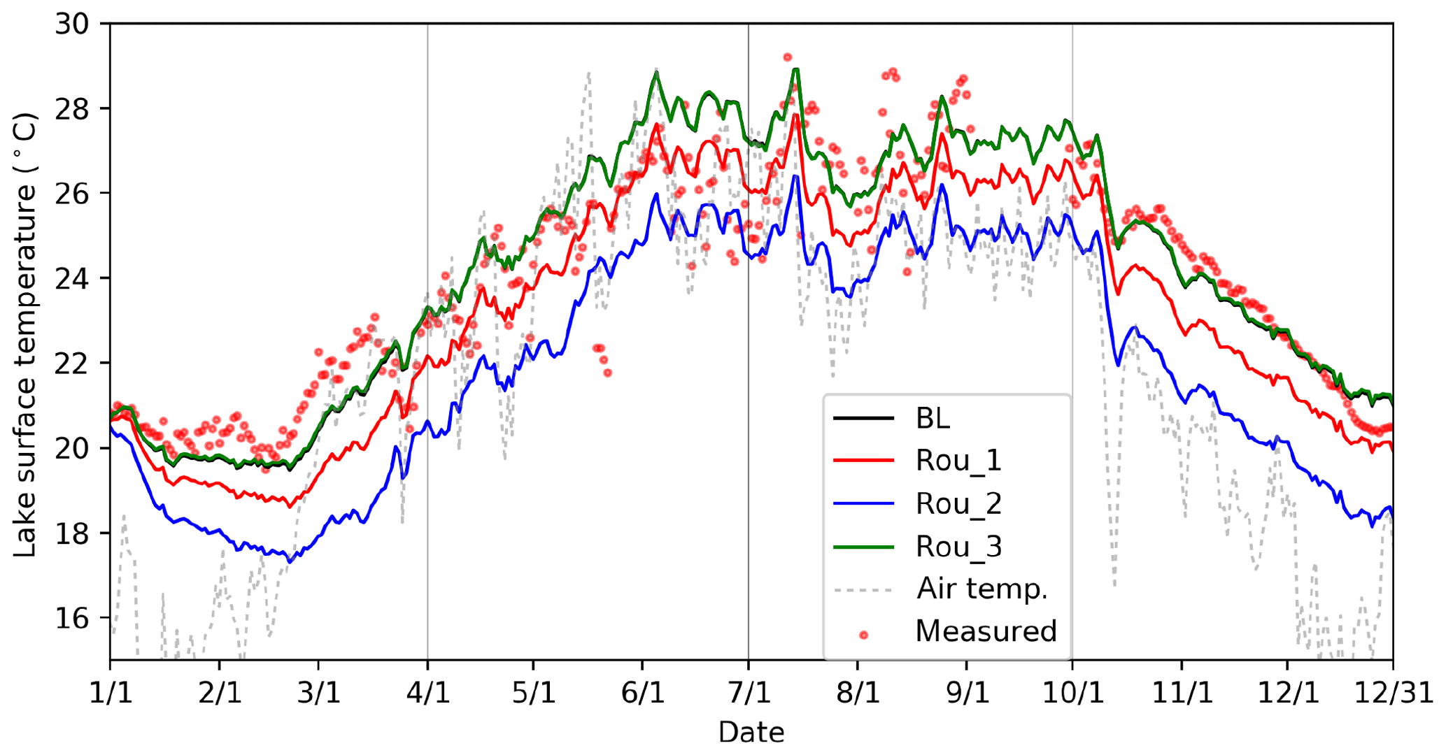
https://www.geosci-model-dev.net/12/2119/2019/gmd-12-2119-2019-f10

Figure 10Time series of LST by observation (red dots), BL (black line), Rou_1 (red line), Rou_2 (blue line), Rou_3 (green line), and air temperature (gray dashed line) of Nuozhadu Reservoir in the year 2015. Note that BL and Rou_3 overlap most of the time.

Download

When the roughness lengths are fixed to 1 mm (Rou_1), an increase in sensible heat fluxes up to 30 W m⁻² is caused in cold seasons but slight decreases are seen in warm seasons (Fig. 11a). A larger effect is observed in latent heat flux, which is increased throughout the year by up to 30 W m⁻² (Fig. 11b). Annual average LST is reduced by ∼1 ^∘C due to excessive outgoing heat fluxes, mainly the latent heat flux. These effects are amplified when fixing the roughness lengths at 10 mm (Rou_2), resulting in up to 100 W m⁻² increases in winter, 50 W m⁻² decreases in summer for sensible heat fluxes, and up to 200 W m⁻² increases throughout the year for latent heat fluxes. With Rou_2, annual average LST is accordingly reduced by ∼2.5 ^∘C compared to BL.

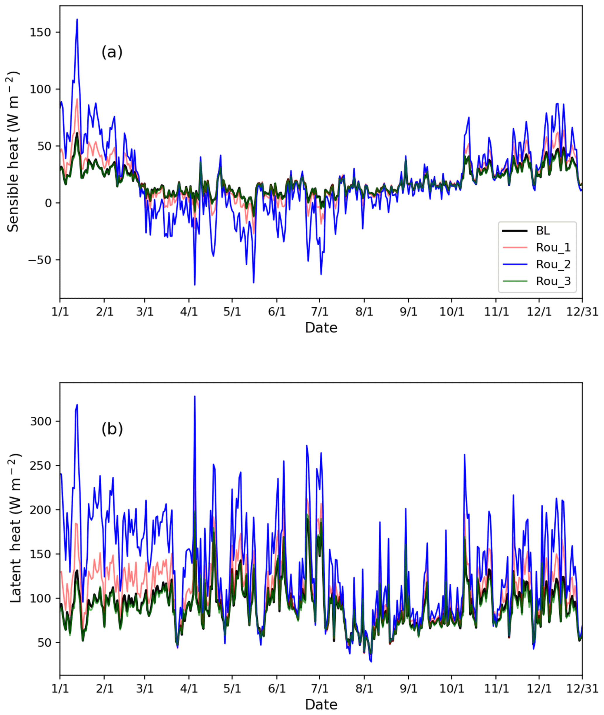
https://www.geosci-model-dev.net/12/2119/2019/gmd-12-2119-2019-f11

Figure 11Time series of (a) upward sensible heat flux, (b) upward latent heat flux by BL (black line), Rou_1 (red line), Rou_2 (blue line), and Rou_3 (green line) of Nuozhadu Reservoir in 2015.

Download

4.5 Effects of light extinction coefficient

The light extinction coefficient is the key parameter controlling the absorption and distribution of solar radiation in the lake body. BL, Ext_1, Ext_2, and Ext_3 form a group of experiments for the extinction coefficient by prescribing it as 1.00, 0.13, 0.30, and 3.00 m⁻¹ respectively. The control of the extinction coefficient over energy distribution is reflected in the monthly averaged vertical temperature profiles (Fig. 12). In general, as the extinction coefficient increases, a larger portion of energy from solar radiation is maintained in the shallow layers, producing shallower stratification. As the extinction coefficient decreases, more solar radiation penetrates to depth, resulting in a better-developed epilimnion (the top-most and well mixed layer in a thermally stratified lake, occurring above the deeper hypolimnion). BL and Ext_3 produced very similar temperature profiles, which indicates that when the extinction coefficient is sufficiently large, increasing it merely brings in marginal influences in the vertical temperature profile. Specifically, for the Nuozhadu Reservoir, the threshold is ∼1.0 m⁻¹.

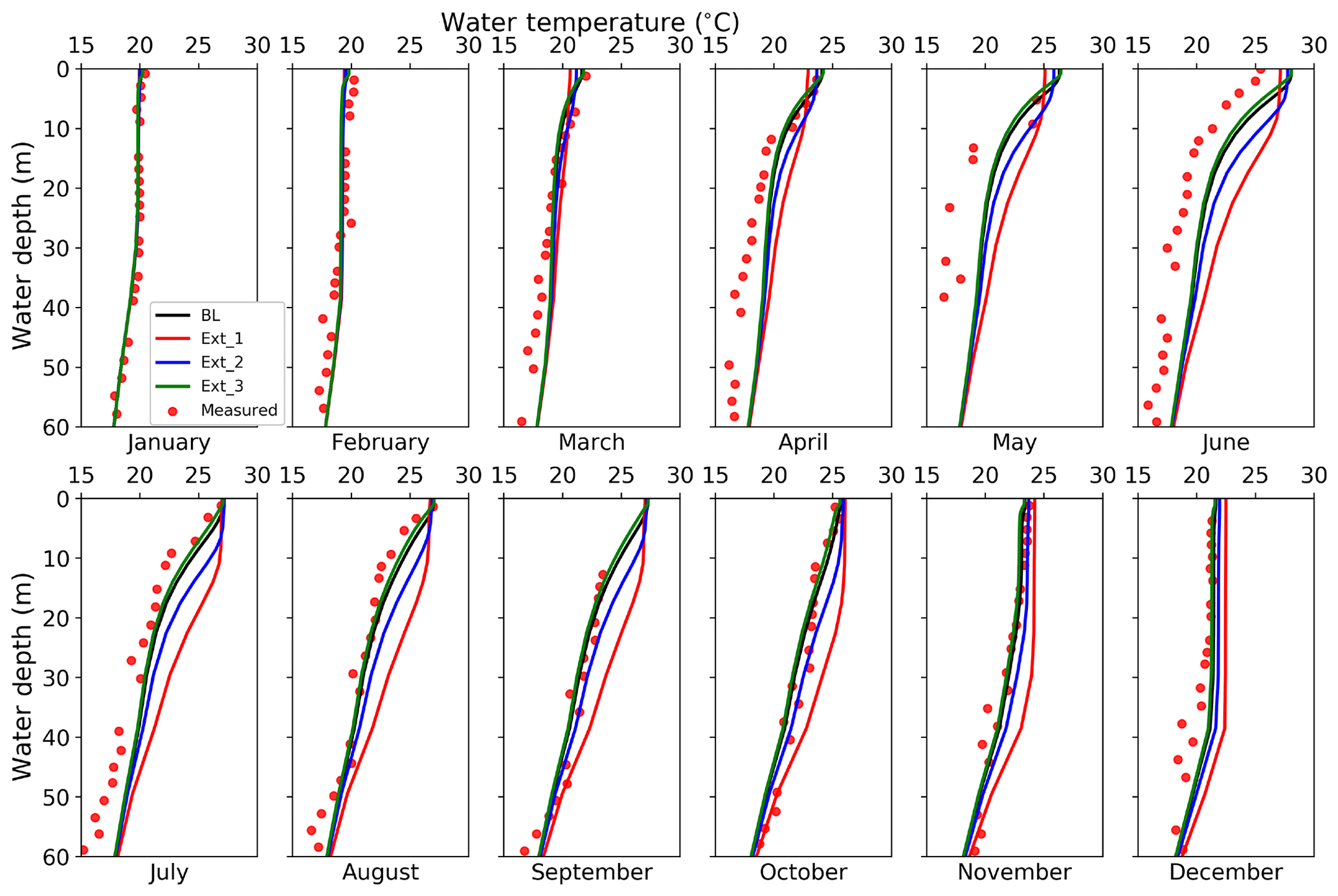
https://www.geosci-model-dev.net/12/2119/2019/gmd-12-2119-2019-f12

Figure 12Monthly vertical temperature profile for the first 60 m water by observation (red dots), BL (black line), Ext_1 (red line), Ext_2 (blue line), and Ext_3 (green line) in the year 2015.

Download

Among the four experiments, Ext_1 applied the default light extinction coefficient by WRF-Lake (the smallest). This allowed solar radiation to penetrated deeper and energy to be distributed more evenly in the lake body, resulting in less temperature stratification in the topmost 10 m almost year-round. The cumulative influence of lower lake opacity in Ext_1 is also well manifested in seasonal LST. In spring and summer, Ext_1 simulated lower LSTs than other scenarios as more solar radiation penetrated into and warmed up deeper layers. Further, with lower LSTs, less sensible and latent heat were dissipated and more energy was maintained within the lake body. By the end of the year, Ext_1 resulted in an integrally warmer water body than other scenarios with higher water temperatures of 1.5–2 ^∘C.

4.6 Uncertainties and limitations

Ice and snow processes could play a significant role in lake–atmosphere interactions (Brown and Duguay, 2010), especially for high-latitude lakes (e.g., north Eurasian lakes, Subin et al., 2012a; Great Lakes, Xiao et al., 2016). However, given the warm climatology of the Nuozhadu Reservoir, we only examined here the performance of WRF-rLake under ice-free conditions. Future work should be carried out to assess WRF-rLake performance at more reservoirs or lakes with ice-covered periods as well as different bathymetry and climate to evaluate the broader model applicability.

Due to the lack of Secchi disk measurements at the Nuozhadu Reservoir, we were unable to further improve the radiation scheme in WRF-rLake. However, we note that lake biology is a dominant factor influencing lake optical properties (Cristofor et al., 1994), which itself is affected by many processes, including lake hydrology and biogeochemistry. As modeling such processes is beyond the scope of the current WRF-rLake module, the parameterization of light extinction in WRF-Lake is simply based on lake depth (Eq. 3). Considering the remarkable impacts of lake opacity on lake energy distribution and mixing regime, future developments should include more sophisticated parameterizations of extinction coefficient with considerations of lake hydrology, chemistry, and biology.

Operation-induced inflows and outflows are key features of artificial reservoirs and can strongly affect seasonal and interannual evolution of reservoir surface water levels, intensity of thermal stratification, and thermal structure (Anohin et al., 2006; Çalışkan and Elçi, 2009). Given that reservoirs are essential infrastructures for the utilization and management of water resources (Jain and Singh, 2003; Ahmad et al., 2014), the WRF-rLake framework should be extended to include reservoir operation features (e.g., inflow and outflow controls) to better characterize reservoir–atmosphere interactions.

5 Conclusions

In this study, we revised the WRF-Lake model by adding a new spatial discretization scheme, modifying surface property and vertical diffusivity parameterizations, and adopting a revised convection scheme. The revised lake model, WRF-rLake, was evaluated at the deep Nuozhadu Reservoir in southwestern China and demonstrated overall improved performance in simulating water temperatures in comparison with WRF-Lake, the current lake model in WRF. Compared to WRF-Lake, WRF-rLake reduced the RMSE against observed lake surface temperatures (LSTs) from 1.35 to 1.14 ^∘C and that against monthly observed lake temperatures profiles from 1.51 to 1.13 ^∘C.

Based on the comparison between WRF-Lake and WRF-rLake, we found that the coarse discretization of water layers in the current WRF-Lake made it less able to accurately predict temperatures in the thermocline. A 25-layer scheme was thus introduced to WRF-rLake and demonstrated better performance than the original 10-layer scheme by reducing the RMSE against observed lake temperatures profiles from 1.64 to 1.13 ^∘C.

In WRF-Lake, the lake surface roughness length is prescribed to be 1 mm, which we found led to biased simulated surface fluxes and surface temperatures. Lakes have much smoother surfaces, and thus smaller roughness lengths, compared to land and oceans, and lake roughness lengths vary with wind and surface waves. Replacing the original parameterization of roughness lengths with our proposed parameterization (Eqs. 5, 6, 7, 8) reduced latent heat flux by up to 30 W m⁻², and considerably improved LST simulations by reducing the RMSE against observations from 1.34 to 1.14 ^∘C.

Simulations of temperature stratification and surface fluxes are sensitive to lake opacity, which modulates the absorption of solar radiation in the lake body. Considering that lake opacity may vary by more than 2 orders of magnitude (Subin et al., 2012a), more detailed global datasets on lake opacity based on remote sensing should be developed. Field measurements of extinction coefficients will be critical for achieving high-quality weather and climate simulations in lake-rich areas.

Previous studies have recognized that the wind-driven eddy diffusivity parameterization by Hostetler and Bartlein (1990) is insufficient to simulate large and deep lake surface fluxes and water temperatures. Gu et al. (2015) therefore increased eddy diffusivity for deep lakes with large multiplicative factors that depend on lake depth and surface temperature. However, we found such treatment resulted in unrealistically large eddy diffusivity in about the top 10 m of the Nuozhadu Reservoir and failed to compensate for the unresolved 3-D mixing processes in deeper layers. WRF-rLake thus adopts a maximum of 10² cm² s⁻¹ for eddy diffusivity to avoid overestimation in the surface layers and an enhanced diffusion term for deep lakes, resulting in more realistic eddy diffusivities in deeper layers. In the case of the Nuozhadu Reservoir, adopting all the modifications to eddy diffusivity produced overall similar diffusivity to those measured in Lake Zürich (a lake with similar topography and depth). Although considerable improvements have been brought in by WRF-rLake, the parameterization for vertical diffusivity should be further evaluated and improved to resolve remaining uncertainties in its performance at other lakes, especially for deep lakes. We note several other limitations that could guide future work, e.g., the need to evaluate ice and snow processes and to improve the radiation scheme and the inflow–outflow parameterization. Our future work will couple the WRF-rLake module with the WRF framework to examine the performance of the coupled system. Overall, we find that simulations of lake temperatures and surface energy balances were improved by WRF-rLake by modifications to the discretization scheme, lake opacity, parameterization for surface properties and vertical diffusivity, and convection scheme.

Code and data availability

The WRF-rLake source code (under MIT license) with a sample dataset is provided in Wang et al. (2019). Instructions for running the offline model can also be found in README.md via the above link. The whole dataset used in this paper is available upon request to Ting Sun (ting.sun@reading.ac.uk).

Appendix A: Parameterization for wind-driven eddy diffusivity

In the Henderson-Sellers parameterization scheme, wind-driven eddy diffusivity (k_e) is determined by wind speed at 2 m above the water surface, a latitude-dependent Ekman profile, and a lake-stratification-dependent Brunt–Väisälä frequency (Henderson-Sellers et al., 1983; Henderson-Sellers, 1985):

\begin{matrix} (A1) & k_{e} = (k u_{*} z / P_{0}) e^{(- k^{*} z)} {(1 + 37 {Ri}^{2})}^{- 1}, \end{matrix}

where k(=0.4) is von Kármán's constant, u_* is the surface friction velocity (m s⁻²), P₀(=1.0) is the neutral value of the turbulent Prandtl number, k^* is a latitudinally dependent parameter of the Ekman profile, and Ri is the gradient Richardson number.

The parameter u_* is given by the following:

\begin{matrix} (A2) & u_{*} = 1.2 \times 10^{- 3} u, \end{matrix}

where u (m s⁻¹) is wind speed at 2 m a.g.l.

The parameter k^* is expressed as follows:

\begin{matrix} (A3) & k^{*} = 6.6 \times {(\sin ϕ)}^{1 / 2} u^{- 1.84}, \end{matrix}

where ϕ is the latitude of the lake being modeled.

The parameter Ri is determined as follows:

\begin{matrix} (A4) & Ri = \frac{- 1 + {\{1 + 40 N^{2} k^{2} z^{2} / [u_{*}^{2} \exp (- 2 k^{*} z)]\}}^{1 / 2}}{20}, \end{matrix}

where N (s⁻¹) is the Brunt–Väisälä frequency specified as follows:

\begin{matrix} (A5) & N = {[- g / ρ (\partial ρ / \partial z)]}^{1 / 2} . \end{matrix}

Author contributions

FW and TS coded the revised model. GN, DZ, and TS designed the project that supports this study. WJR, JT, and FW designed numerical experiments. DZ provided measurements of Nuozhadu Reservoir for model evaluation. FW led the manuscript preparation with contributions from all other authors.

Competing interests

The authors declare that they have no conflict of interest.

Acknowledgements

We thank Huaneng Lancang River Hydropower Inc. for their support with measurements at the Nuozhadu Reservoir. We appreciate two anonymous reviewers and the editor James R. Maddison for their comments and suggestions that significantly improved the quality of this work.

Financial support

Fushan Wang, Guangheng Ni, and Dejun Zhu are supported by the National Natural Science Foundation of China (NSFC, grant nos. 51679119 and 91647107). Jinyun Tang and William J. Riley are supported by the Director, Office of Science, Office of Biological and Environmental Research of the US Department of Energy under contract no. DE-AC02-05CH11231 as part of the Regional and Global Climate Modeling (RGCM) Program. Ting Sun is supported by the UKRI NERC Independent Research Fellowship (grant no. NE/P018637/1).

Review statement

This paper was edited by James R. Maddison and reviewed by two anonymous referees.

References

Ahmad, A., El-Shafie, A., Razali, S. F. M., and Mohamad, Z. S.: Reservoir Optimization in Water Resources: a Review, Water Resour. Manag., 28, 3391–3405, https://doi.org/10.1007/s11269-014-0700-5, 2014.

Anohin, V. V., Imberger, J., Romero, J. R., and Ivey, G. N.: Effect of long internal waves on the quality of water withdrawn from a stratified reservoir, J. Hydraul. Eng.-ASCE, 132, 1134–1145, 2006.

Ataktürk, S. S. and Katsaros, K. B.: Wind Stress and Surface Waves Observed on Lake Washington, J. Phys. Oceanogr., 29, 633–650, 1999.

Bates, G. T., Giorgi, F., and Hostetler, S. W.: Toward the simulation of the effects of the Great Lakes on regional climate, Mon. Weather Rev., 121, 1373–1387, 1993.

Bates, G. T., Hostetler, S. W., and Giorgi, F.: Two-Year Simulation of the Great Lakes Region with a Coupled Modeling System, Mon. Weather Rev., 123, 1505–1522, 1995.

Bonan, G. B.: Sensitivity of a GCM simulation to inclusion of inland water surfaces, J. Chem. Ecol., 8, 2691—2704, 1995.

Burchard, H., Bolding, K., and Villarreal, M. R.: GOTM, a General Ocean Turbulence Model: theory, implementation and test cases, Space Applications Institute, Ispra, Italy, 1999.

Çalışkan, A. and Elçi, S. : Effects of selective withdrawal on hydrodynamics of a stratified reservoir, Water Resour. Manag., 23, 1257–1273, 2009.

Charnock, H.: Wind stress over a water surface, Q. J. Roy. Meteor. Soc., 81, 639–640, 1955.

Chen, Y., Yang, K., He, J., Qin, J., Shi, J., Du, J., and He, Q.: Improving land surface temperature modeling for dry land of China, J. Geophys. Res., 116, D20104, https://doi.org/10.1029/2011jd015921, 2011.

Cristofor, S., Vadineanu, A., Ignat, G., and Ciubuc, C.: Factors affecting light penetration in shallow lakes, Hydrobiologia, 275–276, 493–498, 1994.

Deng, B., Liu, S., Xiao, W., Wang, W., Jin, J., and Lee, X.: Evaluation of the CLM4 lake model at a large and shallow freshwater lake, J. Hydrometeorol., 14, 636–649, 2013.

Dutra, E., Stepanenko, V. M., Balsamo, G., Viterbo, P., Miranda, P. M. A., Mironov, D., and Schär, C.: An offline study of the impact of lakes on the performance of the ECMWF surface scheme, Boreal Environ. Res., 15, 100–112, 2010.

Ellis, C. R.: Water temperature dynamics and heat transfer beneath the ice cover of a lake, Limnol. Oceanogr., 36, 324–334, 1991.

Engineering Sciences Data Unit (ESDU): Characteristics of Wind Speed in the Lower Layers of the Atmosphere Near the Ground: Strong Winds (Neutral Atmosphere), ESDU Data Item No. 72026, ESDU, Regent Street, London, UK, 1972.

Fairall, C. W., Bradley, E. F., Rogers, D. P., Edson, J. B., and Young, G. S.: Bulk parameterization of air-sea fluxes for Tropical Ocean-Global Atmosphere Coupled-Ocean Atmosphere Response Experiment, J. Geophys. Res., 101, 3747–3764, 1996.

Fang, X. and Stefan, H. G.: Long-term lake water temperature and ice cover simulations/measurements, Cold Reg. Sci. Technol., 24, 289–304, 1996.

Goudsmit, G.-H., Burchard, H., Peeters, F., and Wüest, A.: Application of k–ϵ turbulence models to enclosed basins: The role of internal seiches, J. Geophys. Res., 107, 3230, https://doi.org/10.1029/2001JC000954, 2002.

Gu, H., Jin, J., Wu, Y., Ek, M. B., and Subin, Z. M.: Calibration and validation of lake surface temperature simulations with the coupled WRF-lake model, Climatic Change, 129, 471–483, https://doi.org/10.1007/s10584-013-0978-y, 2015.

Gu, H., Ma, Z., and Li, M.: Effect of a large and very shallow lake on local summer precipitation over the Lake Taihu basin in China, J. Geophys. Res.-Atmos., 121, 8832–8848, https://doi.org/10.1002/2015jd024098, 2016.

Gula, J. and Peltier, W. R.: Dynamical downscaling over the Great Lakes basin of North America using the WRF regional climate model: the impact of the Great Lakes system on regional greenhouse warming, J. Climate, 25, 7723–7742, 2012.

Håkanson, L.: Models to predict Secchi depth in small glacial lakes, Aquat. Sci., 57, 31–53, 1995.

Harris, L. M., Lin, S.-J., and Tu, C.: High-Resolution Climate Simulations Using GFDL HiRAM with a Stretched Global Grid, J. Climate, 29, 4293–4314, https://doi.org/10.1175/jcli-d-15-0389.1, 2016.

Henderson-Sellers, B.: New formulation of eddy diffusion thermocline models, Appl. Math. Model., 9, 441–446, 1985.

Henderson-Sellers, B., Mccormick, M. J., and Scavia, D.: A comparison of the formulation for eddy diffusion in two one-dimensional stratification models, Appl. Math. Model., 7, 212–215, 1983.

Hocking, G. C. and Straškraba, M.: The effect of light extinction on thermal stratification in reservoirs and lakes, Int. Rev. Hydrobiol., 84, 535–556, 2015.

Hondzo, M., and Stefan, H. G.: Lake Water Temperature Simulation Model, J. Hydraul. Eng.-ASCE, 119, 1251–1273, 1993.

Hostetler, S. W. and Bartlein, P. J.: Simulation of lake evaporation with application to modeling lake level variations of Harney-Malheur Lake, Oregon, Water Resour. Res., 26, 2603–2612, 1990.

Hostetler, S. W. and Giorgi, F.: Effects of a 2×CO₂, climate on two large lake systems: Pyramid Lake, Nevada, and Yellowstone Lake, Wyoming, Global Planet. Change, 10, 43–54, 1995.

Hostetler, S. W., Giorgi, F., Bates, G. T., and Bartlein, P. J.: Lake-atmosphere feedbacks associated with paleolakes Bonneville and Lahontan, Science, 263, 665–668, 1994.

Hutchinson, G. E.: A treatise on limnology v.1, John Wiley, John Wiley & Sons, Inc., Hoboken, United States, 1957.

Imberger, J., Patterson, J., Hebbert, B., and Loh, I.: Dynamics of reservoir of medium size, J. Hydr. Div.-ASCE, 104, 725–743, 1978.

Jain, S. K. and Singh, V. P.: Water resources systems planning and management, Elsevier, Amsterdam, 2003.

Jassby, A. and Powell, T.: Vertical patterns of eddy diffusion during stratification in Castle Lake, California1, Limnol. Oceanogr., 20, 530–543, 1975.

Jerlov, N. G.: Marine optics, Elsevier Scientific Publishing Company, Amsterdam, The Netherlands, 231 pp., 1976.

Karagounis, I., Trösch, J., and Zamboni, F.: A coupled physical-biochemical lake model for forecasting water quality, Aquat. Sci., 55, 87–102, 1993.

Kraus, E. B. and Turner, J. S.: A one-dimensional model of the seasonal thermocline II. The general theory and its consequences, Tellus, 19, 98–106, 1967.

Krinner, G.: Impact of lakes and wetlands on boreal climate, J. Geophys. Res., 108, 4520, https://doi.org/10.1029/2002JD002597, 2003.

Kullenberg, G., Murthy, C., and Westerbuy, H.: An experimental study of diffusion characteristics in the thermocline and hypolimnion regions of Lake Ontario, IEEE, 7, 739–751, 1973.

Kullenberg, G.: An experimental and theoretical investigation of the turbulent diffusion in the upper layer of the sea, J. Mod. Greek Stud., 18, 151–160, 1974.

Lerman, A. and Chou, L.: Physics and chemistry of lakes with 48 tables, Springer, Berlin, 2013.

Li, Y. H.: Vertical eddy diffusion coefficient in Lake Zürich, Schweiz. Z. Hydrol., 35, 1–7, 1973.

Li, Z., Lyu, S., Zhao, L., Wen, L., Ao, Y., and Wang, S.: Turbulent transfer coefficient and roughness length in a high-altitude lake, Tibetan Plateau, Theor. Appl. Climatol., 124, 723–735, https://doi.org/10.1007/s00704-015-1440-z, 2015.

Lofgren, B. M.: Simulated effects of idealized Laurentian great lakes on regional and large-scale climate, J. Climate, 10, 2847–2858, 1997.

Long, Z., Perrie, W., Gyakum, J., Caya, D., and Laprise, R.: Northern lake impacts on local seasonal climate, J. Hydrometeorol., 8, 881–896, 2007.

MacKay, M. D., Neale, P. J., Arp, C. D., De Senerpont Domis, L. N., Fang, X., Gal, G., Jöhnk, K. D., Kirillin, G., Lenters, J. D., Litchman, E., MacIntyre, S., Marsh, P., Melack, J., Mooij, W. M., Peeters, F., Quesada, A., Schladow, S. G., Schmid, M., Spence, C., and Stokesr, S. L.: Modeling lakes and reservoirs in the climate system, Limnol. Oceanogr., 54, 2315–2329, 2009.

Mallard, M. S., Nolte, C. G., Spero, T. L., Bullock, O. R., Alapaty, K., Herwehe, J. A., Gula, J., and Bowden, J. H.: Technical challenges and solutions in representing lakes when using WRF in downscaling applications, Geosci. Model Dev., 8, 1085–1096, https://doi.org/10.5194/gmd-8-1085-2015, 2015.

Mallard, M. S., Nolte, C. G., Bullock, O. R., Spero, T. L., and Gula, J.: Using a coupled lake model with WRF for dynamical downscaling, J. Geophys. Res., 119, 7193–7208, https://doi.org/10.1002/2014JD021785, 2014.

Martynov, A., Sushama, L., and Laprise, R.: Simulation of temperate freezing lakes by one-dimensional lake models: Performance assessment for interactive coupling with regional climate models, Boreal Environ. Res., 15, 143–164, 2010.

Mironov, D., Kourzeneva, E., Ritter, B., and Schneider, N.: Implementation of the lake parameterisation scheme Flake into numerical weather prediction model COSMO, Boreal Environ. Res., 15, 77–95, 2010.

Niziol, T. A., Snyder, W. R., and Waldstreicher, J.S.: Winter weather forecasting throughout the eastern United States. IV: lake effect snow, Weather Forecast., 10, 61–77, 1995.

Notaro, M., Holman, K., Zarrin, A., Fluck, E., Vavrus, S. J., and Bennington, V.: Influence of the Laurentian Great Lakes on regional climate, J. Climate, 26, 789–804, 2013.

Oleson, K. W., Lawrence, D. M., Bonan, G. B., Flanner, M. G., Kluzek, E., Lawrence, P. J., Levis, S., Swenson, S. C., Thornton, P. E., Dai, A., Decker, M., Dickinson, R., Feddema, J., Heald, C. L., Hoffman, F., Lamarque, J.-F., Mahowald, N., Niu, G.-Y., Qian, T., Randerson, J., Running, S., Sakaguchi, K., Slater, A., Stöckli, R., Wang, A., Yang, Z.-L., Zeng, X., and Zeng, X.: Technical description of version 4.0 of the Community Land Model (CLM), NCAR Technical Note NCAR/TN-478+STR, National Center for Atmospheric Research, Boulder, CO, 257 pp., 2010.

Oleson, K. W., Lawrence, D. M., Bonan, G. B., Drewniak, B., Huang, M., Koven, C. D., Levis, S., Li, F., W. J., Riley, Subin, Z. M., Swenson, S. C., Thornton, P. E., Bozbiyik, A., Fisher, R., Heald, C. L., Kluzek, E., Lamarque, J.-F., Lawrence, P. J., Leung, L. R., Lipscomb, W., Muszala, S., and Ricciuto, D. M.: Technical Description of version 4.5 of the Community Land Model (CLM), NCAR Technical Note NCAR/TN-503+STR, National Center for Atmospheric Research, Boulder, CO, 422 pp., 2013.

Paulson, C. A. and Simpson, J. J.: The temperature difference across the cool skin of the ocean, J. Geophys. Res., 86, 11044–11054, https://doi.org/10.1029/jc086ic11p11044, 1981.

Peeters, F., Livingstone, D. M., Goudsmit, G., Kipfer, R., and Forster, R.: Modeling 50 years of historical temperature profiles in a large central European lake, Limnol. Oceanogr., 47, 186–197, 2002.

Perroud, M., Goyette, S., Martynov, A., Beniston, M., and Anneville, O.: Simulation of multiannual thermal profiles in deep Lake Geneva: a comparison of one-dimensional lake models, Limnol. Oceanogr., 54, 1574–1594, 2009.

Quay, P. D., Broecker, W. S., Hesslein, R. H., and Schindler, D. W.: Vertical diffusion rates determined by tritium tracer experiments in the thermocline and hypolimnion of two lakes, Limnol. Oceanogr., 25, 201–218, 1980.

Riley, M. J. and Stefan, H. G.: Minlake: A dynamic lake water quality simulation model, Ecol. Model., 43, 155–182, 1988.

Samuelsson, P., Kourzeneva, E., and Mironov, D.: The impact of lakes on the European climate as simulated by a regional climate model, Boreal Environ. Res., 15, 113–129, 2010.

Sarmiento, J. L., Feely, H. W., Moore, W. S., Bainbridge, A. E., and Broecker, W. S.: The relationship between vertical eddy diffusion and buoyancy gradient in the deep sea, Earth Planet. Sc. Lett., 32, 357–370, 1976.

Scott, R. W. and Huff, F. A.: Impacts of the great lakes on regional climate conditions, J. Great Lakes Res., 22, 845–863, 1996.

Shen, C.: Accumulation impact on water temperature in a south-north dammed river – A case study in the middle and lower reaches of Lancang river, Report, Tsinghua University, Beijing, 2017 (in Chinese).

Skamarock, W. C., Duda, M. G., Ha, S., and Park, S.-H.: Limited-Area Atmospheric Modeling Using an Unstructured Mesh, Mon. Weather Rev., 146, 3445–3460, https://doi.org/10.1175/mwr-d-18-0155.1, 2018.

Small, E. E., Sloan, L. C., Hostetler, S., and Giorgi, F.: Simulating the water balance of the Aral Sea with a coupled regional climate-lake model, J. Geophys. Res., 104, 6583–6602, 1999.

Smith, I. R.: Hydraulic conditions in isothermal lakes, Freshwater Biol., 9, 119–145, 1979.

Smith, S. D.: Coefficients for sea surface wind stress, heat flux, and wind profiles as a function of wind speed and temperature, J. Geophys. Res., 93, 15467–15472, 1988.

Stepanenko, V. M. and Lykossov, V. N.: Numerical modeling of heat and moisture transfer processes in a system lake–soil, Russ. J. Meteorol. Hydrol., 3, 95–104, 2005.

Stepanenko, V. M., Goyette, S., Martynov, A., Perroud, M., Fang, X., and Mironov, D.: First steps of a lake model intercomparison project: lakemip, Boreal Environ. Res., 15, 191–202, 2010.

Stepanenko, V. M., Machul'Skaya, E. E., Glagolev, M. V., and Lykossov, V. N.: Numerical modeling of methane emissions from lakes in the permafrost zone, Izv. Atmos. Ocean. Phy., 47, 252–264, 2011.

Stepanenko, V. M., Martynov, A., Jöhnk, K. D., Subin, Z. M., Perroud, M., Fang, X., Beyrich, F., Mironov, D., and Goyette, S.: A one-dimensional model intercomparison study of thermal regime of a shallow, turbid midlatitude lake, Geosci. Model Dev., 6, 1337–1352, https://doi.org/10.5194/gmd-6-1337-2013, 2013.

Subin, Z. M., Riley, W. J., and Mironov, D.: An improved lake model for climate simulations: model structure, evaluation, and sensitivity analyses in CESM1, J. Adv. Model. Earth Sy., 4, M02001, https://doi.org/10.1029/2011MS000072, 2012a.

Subin, Z. M., Murphy, L. N., Li, F., Bonfils, C., and Riley, W. J.: Boreal lakes moderate seasonal and diurnal temperature variation and perturb atmospheric circulation: analyses in the Community Earth System Model 1 (CESM1), Tellus A, 64, 53–66, 2012b.

Subin, Z. M., Koven, C. D., Riley, W. J., Torn, M. S., Lawrence, D. M., and Swenson, S. C.: Effects of soil moisture on the responses of soil temperatures to climate change in cold regions, J. Climate, 26, 3139–3158, 2013.

Svensson, U.: A mathematical model of the seasonal thermocline, Phd thesis, Lund Institute of Technology, 1978.

Ulrich, M.: Modeling of chemicals in lakes – development and application of user-friendly simulation software (MASAS & CHEMSEE) on personal computers, PhD thesis, ETH Zürich, No. 9632, https://doi.org/10.3929/ethz-a-000626302, 1991.

Wang, F., Ni, G., Riley, W. J., Tang, J., Zhu, D., and Sun, T.: Code and sample data for GMD paper (https://doi.org/10.5194/gmd-2018-168), Zenodo, https://doi.org/10.5281/zenodo.2624892, 2019.

Wright, D. M., Posselt, D. J., and Steiner, A. L.: Sensitivity of lake-effect snowfall to lake ice cover and temperature in the Great Lakes region, Mon. Weather Rev., 141, 670–689, 2013.

Xiao, C., Lofgren, B. M., Wang, J., and Chu, P. Y.: Improving the lake scheme within a coupled WRF-lake model in the Laurentian great lakes, J. Adv. Model. Earth Sy., 8, 1969–1985, 2016.

Yang, K., Jie, H., Tang, W., Qin, J., and Cheng, C. C. K.: On downward shortwave and longwave radiations over high altitude regions: observation and modeling in the Tibetan Plateau, Agr. Forest Meteorol., 150, 38–46, 2010.

Zamboni, F., Barbieri, A., Polli, B., Salvadè, G., and Simona, M.: The dynamic model SEEMOD applied to the southern basin of lake Lugano, Aquat. Sci., 54, 367–380, 1992.

Zhao, L., Jin, J., Wang, S., and Ek, M. B.: Integration of remote-sensing data with WRF to improve lake-effect precipitation simulations over the Great Lakes region, J. Geophys. Res., 117, D09102, https://doi.org/10.1029/2011JD016979, 2012.

For a reservoir which controls its outflow by movable gates wholly or partially, the term “normal water level” refers to the maximum level that the water may reach under normal operating conditions.

Articles

Short summary

The current lake model in the Weather Research and Forecasting system was reported to be insufficient in simulating deep lakes and reservoirs. We thus revised the lake model by improving its spatial discretization scheme, surface property parameterization, diffusivity parameterization, and convection scheme. The revised model was evaluated at a deep reservoir in southwestern China and the results were in good agreement with measurements.