the Creative Commons Attribution 4.0 License.
the Creative Commons Attribution 4.0 License.
 | 03 Jun 2019
The Monash Simple Climate Model experiments (MSCM-DB v1.0): an interactive database of mean climate, climate change, and scenario simulations
Dietmar Dommenget
Kerry Nice
Tobias Bayr
Dieter Kasang
Christian Stassen
Michael Rezny
This study introduces the Monash Simple Climate Model (MSCM) experiment database. The simulations are based on the Globally Resolved Energy Balance (GREB) model to study three different aspects of climate model simulations: (1) understanding processes that control the mean climate, (2) the response of the climate to a doubling of the CO2 concentration, and (3) scenarios of external forcing (CO2 concentration and solar radiation). A series of sensitivity experiments in which elements of the climate system are turned off in various combinations are used to address (1) and (2). This database currently provides more than 1300 experiments and has an online web interface for fast analysis and free access to the data. We briefly outline the design of all experiments, give a discussion of some results, put the findings into the context of previously published results from similar experiments, discuss the quality and limitations of the MSCM experiments, and also give an outlook on possible further developments. The GREB model simulation is quite realistic, but the model without flux corrections has a root mean square error in the mean state of the surface temperature of about 10 ∘C, which is larger than those of general circulation models (2 ∘C). It needs to be noted here that the GREB model does not simulate circulation changes or changes in cloud cover (feedbacks). However, the MSCM experiments show good agreement to previously published studies. Although GREB is a very simple model, it delivers good first-order estimates, is very fast, highly accessible, and can be used to quickly try many different sensitivity experiments or scenarios. It builds a basis on which conceptual ideas can be tested to first order and it provides a null hypothesis for understanding complex climate interactions in the context of response to external forcing or interactions in the climate subsystems.
- Article
(10274 KB) -
Supplement
(1555 KB) - BibTeX
- EndNote


Our understanding of the dynamics of the climate system and climate changes is strongly linked to the analysis of model simulations of the climate system using a range of climate models that vary in complexity and sophistication. Climate model simulations help us to predict future climate changes and they help us to gain a better understanding of the dynamics of this complex system.
State-of-the-art climate models, such as those used in the Coupled Model Intercomparison Project (CMIP; Taylor et al., 2012), are highly complex simulations that require significant amounts of computing resources and time. Such model simulations require a significant amount of preparation. The development of idealized experiments that would help in the understanding and modelling of climate system processes is often difficult to realize with complex CMIP-type climate models. In this context, simplified climate models are useful, as they provide a fast first guess that helps to inform more complex models. They also help in understanding interactions in the complex system.
In this article, we introduce the Monash Simple Climate Model (MSCM) database (version: MSCM-DB v1.0). The MSCM is an interactive website (http://mscm.dkrz.de for Germany, last access: 22 May 2018; and http://monash.edu/research/simple-climate-model for Australia, last access: 22 May 2018) and database that provides access to a series of more than 1300 experiments with the Globally Resolved Energy Balance (GREB) model (Dommenget and Floter, 2011; hereafter referred to as DF11). The GREB model was primarily developed to conceptually understand the physical processes that control the global warming pattern in response to an increase in CO2 concentration. It therefore centres around the surface temperature (Tsurf) tendency equation and only simulates the processes and variables needed for resolving the global warming pattern.
Simplified climate models, such as Earth system models of intermediate complexity (EMICs), often aim at reducing the complexity to increase computation speed and therefore allow for faster model simulations (e.g. CLIMBER – Petoukhov et al., 2000; UVic – Weaver et al., 2001; FAMOUS – Smith et al., 2008; LOVECLIM – Goosse et al., 2010). These EMICs are very similar in structure to state-of-the-art coupled general circulation models (CGCMs), following the approach of simulating geophysical fluid dynamics. The GREB model differs in that it follows an energy balance approach and does not simulate the geophysical fluid dynamics of the atmosphere. It is therefore a climate model that does not include weather dynamics but focusses on the long-term mean climate and its response to external boundary changes. It also does not include cloud feedbacks or adjustments in the atmospheric circulation, as both are given as boundary conditions. However, it does include the most important water vapour, black-body radiation, and ice–albedo feedbacks.
The purposes of the MSCM database for research studies are the following.
-
First guess: The MSCM provides first guesses for how the climate may change in idealized or realistic experiments. The MSCM experiments can be used to test ideas before implementing and testing them in more detailed CGCM simulations.
-
Null hypothesis: The simplicity of the GREB model provides a good null hypothesis for understanding the climate system. Because it does not simulate weather dynamics or circulation changes on a large or small scale, it provides the null hypothesis of a climate as a pure energy balance problem.
-
Conceptual understanding: The simplicity of the GREB model helps us to better understand the interactions in the complex climate and therefore helps to formulate simple conceptual models for climate interactions.
-
Education: Studying the results of the MSCM helps us to understand the interactions that control the mean state of the climate and its regional and seasonal differences. It helps us to understand how the climate will respond to external forcings in a first-order approximation.
The MSCM provides interfaces for fast analysis of experiments and selection of data (see Figs. 1–3). It is designed for teaching and outreach purposes but also provides a useful tool for researchers. The focus in this study will be on describing the research aspects of the MSCM, whereas the teaching aspects of it will not be discussed. The MSCM experiments focus on three different aspects of climate model simulations: (1) understanding the processes that control the mean climate, (2) the response of the climate to a doubling of the CO2 concentration, and (3) scenarios of external CO2 concentration and solar radiation forcings. We will provide a short outline of the design of all experiments, give a brief discussion of some results, and put the findings into the context of previously published literature results from similar experiments.

Figure 1MSCM interface running the deconstruction of the mean climate experiments. Experiment A, on the left, has all processes turned ON, and experiment B, on the right, has all turned OFF. The Tsurf of experiment A is shown in the upper left map, experiment B in the upper right, and the difference between the two in the lower map. The example shows the values for the October mean.
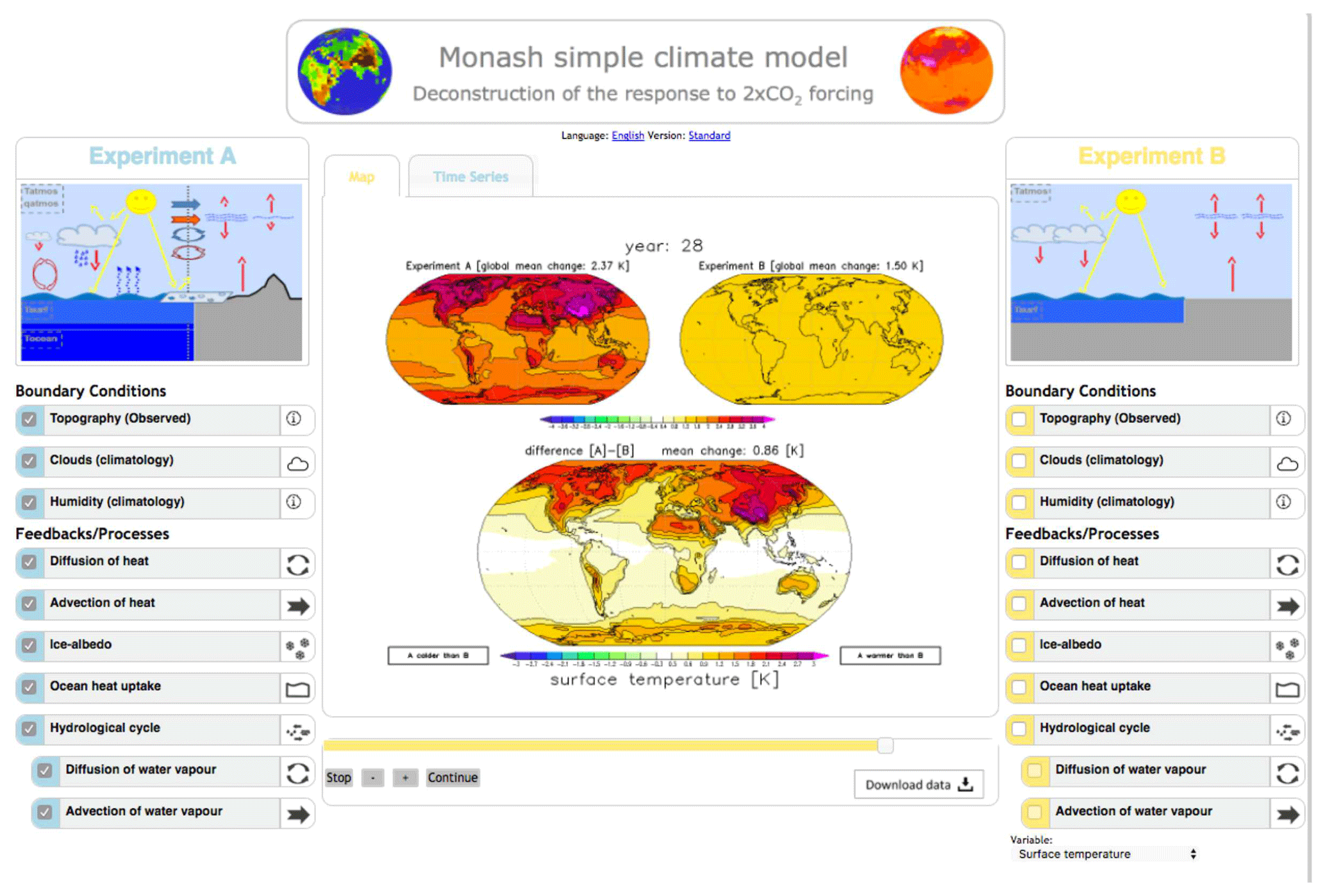
Figure 2MSCM interface running the deconstruction of the response to a doubling of the CO2 concentration in experiments. Experiment A, on the left, has all processes turned ON, and experiment B, on the right, has all turned OFF. The Tsurf response of experiment A is shown in the upper left map, experiment B in the upper right, and the difference between the two in the lower map. The example shows the annual mean values after 28 years.
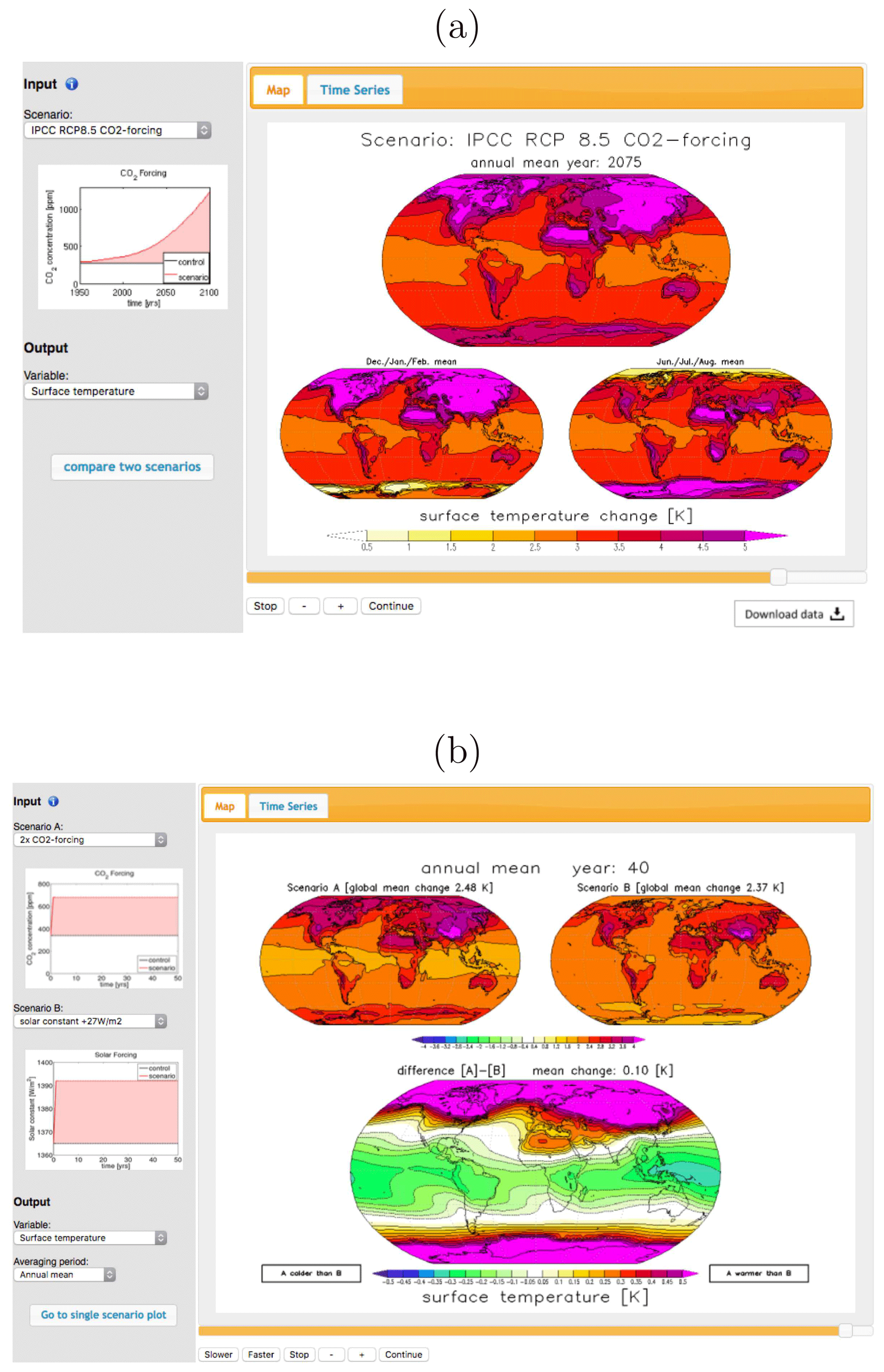
Figure 3Examples of the MSCM scenario interface. (a) A single scenario (here RCP8.5 CO2 forcing) and (b) the comparison of two different scenarios (here a CO2 forcing is compared against a change in the solar constant by +27 W m−2).
The DF11 study focussed primarily on the development of the model equations and a discussion of the response pattern to an increase in CO2 concentration. This study will give a more detailed discussion on the performance of the GREB model in simulations of the mean state of the climate and a wider range of external forcing scenarios, including solar radiation changes.
The paper is organized as follows: the following section describes the GREB model, the experiment designs, the MSCM interface, and the input data used. A short analysis of the experiments is given in Sect. 3. This section will mostly focus on the GREB model performance in comparison to observations and previously published simulations in the literature, but it will also give some indications of the findings in the model experiments and the limitations of the GREB model. The final section will give a short summary and outlook for potential future developments and analysis.
The GREB model is the underlying modelling tool for the MSCM interface. The development of the model and all equations have been presented in DF11. The model is simulating the global climate on a horizontal grid of 3.75∘ longitude ×3.75∘ latitude and in three vertical layers: surface, atmosphere, and subsurface ocean. It simulates four prognostic variables: surface, atmospheric and subsurface ocean temperature, and atmospheric humidity (column-integrated water vapour); see Appendix Eqs. (A1)–(A4). It further simulates a number of diagnostic variables, such as precipitation and snow–ice cover, resulting from the simulation of the prognostic variables.
The main physical processes that control the surface temperature tendencies are simulated: solar (short-wave) and thermal (long-wave) radiation, the hydrological cycle (including evaporation, moisture transport, and precipitation), horizontal transport of heat, and heat uptake in the subsurface ocean. Atmospheric circulation and cloud cover are seasonally prescribed boundary conditions, and state-independent flux corrections are used to keep the GREB model close to the observed mean climate. Thus, the GREB model does not simulate the atmospheric or ocean circulation and is therefore conceptually very different from CGCM simulations.
The model simulates important climate feedbacks, such as the water vapour and ice–albedo feedback, but an important limitation of the GREB model is that the response to external forcings or model parameter perturbations does not involve circulation or cloud feedbacks (Bony et al., 2006, 2015; Boucher et al., 2013). Circulation and cloud feedbacks alter the climate response to external forcings on a regional and, to a lesser extent, global scale. The experiments of this database neglect any effects resulting from cloud or circulation feedbacks. These experiments should therefore only be considered as first-guess estimates. In the context of some of the results discussed further below we will point out some of the limitations of the GREB model approach.
Input climatologies (e.g. Tsurf or atmospheric humidity) for the GREB model are taken from National Centers for Environmental Protection (NCEP) reanalysis data for 1950–2008 (Kalnay et al., 1996), cloud cover climatology from the International Satellite Cloud Climatology Project (ISCCP) (Rossow and Schiffer, 1991), ocean mixed layer depth climatology from Lorbacher et al. (2006), and topographic data from the ECHAM5 atmosphere model (Roeckner et al., 2003).
GREB does not have any internal (natural) variability since daily weather systems are not simulated. Subsequently, the control climate or response to external forcings can be estimated from one single year. The primary advantages of the GREB model in the context of this study are its simplicity, speed, and low computational cost. A 1-year GREB model simulation can be done on a standard personal computer in about 1 s (about 100 000 simulated years per day). It can do simulations of the global climate much faster than any state-of-the-art climate model and is therefore a good first-guess approach to test ideas before they are applied to more complex CGCMs. A further advantage is the lag of internal variability, which allows for the detection of a response to external forcing much more easily.
2.1 Experiments for the mean climate deconstruction
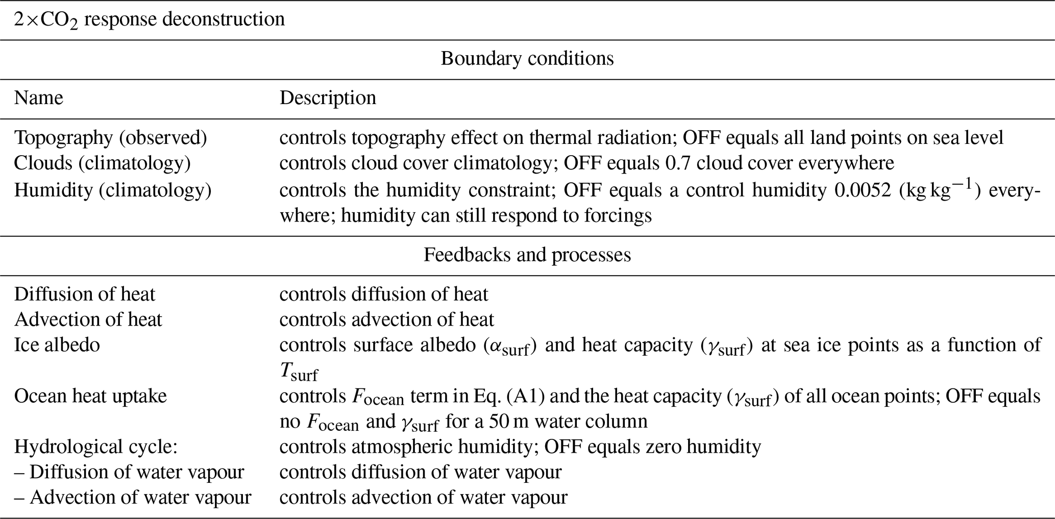
The conceptual deconstruction of the GREB model to understand interactions in the climate system that lead to mean climate characteristics is achieved by defining 11 processes (switches; see Fig. 1). For each of these switches, a term in the model equations is set to zero or altered if the switch is OFF. The processes and how they affect the model equations are briefly listed below (with a short summary in Table 1). The model equations relevant for the experiments in this study are briefly restated in Appendix A1 for the purpose of explaining each experimental set-up in the MSCM.
Table 1Processes (switches) controlled in the sensitivity experiment for the mean climate deconstruction. Indentation in the left column indicates that process switches are dependent on the switches above being ON.

Ice albedo. The surface albedo (αsurf) and the heat capacity over ocean points (γsurf) are influenced by snow and sea ice cover. In the GREB model these are a direct function of Tsurf. When the ice–albedo switch is OFF the surface albedo of all points is constant (0.1), and for ocean points γsurf follows the prescribed ocean mixed layer depth independent of Tsurf (i.e. no ice-covered ocean).
Clouds. The cloud cover, CLD, influences the amount of solar radiation reaching the surface (αclouds in Eq. A5) and the emissivity of the atmospheric layer, εatmos, for thermal radiation (Eq. A8). When the cloud switch is OFF, the cloud cover is set to zero.
Oceans. The ocean in the GREB model simulates subsurface heat storage with the surface mixed layer (∼ upper 50–100 m). When the ocean switch is OFF, the Focean term in Eq. (A1) is set to zero, Eq. (A3) is set to zero, and the heat capacity of all ocean points is set to that of land points.
Atmosphere. The atmosphere in the GREB model simulates a number of processes: the hydrological cycle, horizontal transport of heat, thermal radiation, and sensible heat exchange with the surface. When the atmosphere switch is OFF, Eqs. (A2) and (A4) are set to zero, the heat flux terms, Fsense and Flatent in Eq. (A1) are set to zero, and the downward atmospheric thermal radiation term in Eq. (A6) is set to zero.
Diffusion of heat. The atmosphere transports heat by isotropic diffusion (fourth term in Eq. A2). When this process is switched OFF, the term is set to zero.
Advection of heat. The atmosphere transports heat by advection following the mean wind field, u (fifth term in Eq. A2). When this process is switched OFF, the term is set to zero.
CO2. The CO2 concentration affects the emissivity of the atmosphere, εatmos (Eq. A9). When this process is switched OFF, the CO2 concentration is set to zero.
Hydrological cycle. The hydrological cycle in the GREB model simulates the evaporation, precipitation, and transport of atmospheric water vapour (Eq. A4). It further simulates latent heat cooling at the surface and heating in the atmosphere. When the hydrological cycle is switched OFF, Eq. (A4) is set to zero, the heat flux term Flatent in Eq. (A1) is set to zero, and viwvatmos in Eq. (A9) is set to zero. Subsequently, atmospheric humidity is zero.
It needs to be noted here that the atmospheric emissivity in the log-function parameterization of Eq. (A9) can become negative if the hydrological cycle, cloud cover, and CO2 concentration are switched OFF (set to zero). This marks an unphysical range of the GREB emissivity function and we will discuss the limitations of the GREB model in these experiments in Sect. 3b.
Diffusion of water vapour. The atmosphere transports water vapour by isotropic diffusion (third term in Eq. A4). When this process is switched OFF, the term is set to zero.
Advection of water vapour. The atmosphere transports water vapour by advection following the mean wind field, u (fifth term in Eq. A2). When this process is switched OFF, the term is set to zero.
Model corrections. The model correction terms in Eqs. (A1), (A3), and (A4) artificially force the mean Tsurf, Tocean, and qair climate to be as observed. When the model correction is switched OFF, the three terms are set to zero. This will allow the GREB model to be studied without any artificial corrections and therefore help to evaluate the GREB model equations' skill in simulating climate dynamics.
It should be noted here that the model correction terms in the GREB model have been introduced to study the response to doubling the CO2 concentration for the current climate, which is a relatively small perturbation if compared against the other perturbations considered above. They are meaningful for a small perturbation in the climate system but are less likely to be meaningful with large perturbations to the climate system (e.g. cloud cover set to zero).
Each different combination of the above-mentioned process switches defines a different experiment. However, not all combinations of switches are possible because some of the process switches depend on each other (see Table 1 and Fig. 1). The total number of experiments possible with these process switches is 656. For each experiment, the GREB model is run for 50 years, starting from the original GREB model climatology, and the final year is presented as the climatology of this experiment in the MSCM database.
2.2 Experiments for the 2× CO2 response deconstruction
In a similar way as described above for the mean climate, the climate response to a doubling of the CO2 concentration can be conceptually deconstructed with a set of GREB model experiments. These experiments help us to understand interactions in the climate system that lead to the climate response to a doubling of the CO2 concentration. However, there are a number of differences that need to be considered.
A meaningful deconstruction of the response to a doubling of the CO2 concentration should consider the reference control mean climate since the forcings and the feedbacks controlling the response are mean state dependent. We therefore ensure that all sensitivity experiments in this discussion have the same reference mean control climate. This is achieved by estimating the flux correction term in Eqs. (A1), (A3), and (A4) for each sensitivity experiment to maintain the observed control climate. Thus, when a process is switched OFF, the control climatological tendencies in Eqs. (A1), (S3), and (S4) are the same as in the original GREB model, but changes in the tendencies due to external forcings, such as doubling the CO2 concentration, are not affected by the disabled process. This is the same approach as in DF11.
For the 2×CO2 response deconstruction experiments, we define 10 boundary conditions or processes (switches; see Fig. 2). The ice albedo, advection and diffusion of heat and water vapour, and the hydrological cycle processes are defined in the same way as for the mean climate deconstruction (Sect. 2a). The remaining boundary conditions and processes are briefly listed below (and a short summary is given in Table 2).
Table 2Processes (switches) controlled in the sensitivity experiment for the 2×CO2 response deconstruction. Indentation in the left column indicates that process switches are dependent on the switches above being ON.
The following boundary conditions are considered.
Topography. The topography in the GREB model affects the amount of atmosphere above the surface and therefore affects the emissivity of the atmosphere in the thermal radiation (Eq. A9). Regions with high topography have lower greenhouse gas concentrations in the thermal radiation (Eq. A9). It further affects the diffusion coefficient (κ) for the transport of heat and moisture (Eqs. A2 and A4). When the topography is turned OFF, all points of the GREB model are set to sea level height and have the same amount of CO2 concentration in the thermal radiation (Eq. A9).
Clouds. The cloud cover in the GREB model affects the incoming solar radiation and the emissivity of the atmosphere in the thermal radiation (Eq. A9). In particular, it influences the sensitivity of the emissivity to changes in the CO2 concentration. A clear-sky atmosphere is more sensitive to changes in the CO2 concentration than a fully cloud-covered atmosphere. When the cloud cover switch is OFF, the observed cloud cover climatology boundary conditions are replaced with a constant global mean cloud cover of 0.7. It is not set to zero to avoid an impact on the global climate sensitivity and to focus on the regional effects of inhomogeneous cloud cover.
Humidity. Similarly to the cloud cover, the amount of atmospheric water vapour affects the emissivity of the atmosphere in the thermal radiation and, in particular, the sensitivity to changes in the CO2 concentration (Eq. A9). A humid atmosphere is less sensitive to changes in the CO2 concentration than a dry atmosphere. When the humidity switch is OFF, the constraint to the observed humidity climatology (flux correction in Eq. A4) is replaced with a constant global mean humidity of 0.0052 kg kg−1. It is again not set to zero to avoid an impact on the global climate sensitivity and to focus on the regional effects of inhomogeneous humidity.
The additional feedbacks and processes considered
Ocean heat uptake. The ocean heat uptake in GREB is done in two ocean layers. The largest part of the ocean heat is in the subsurface layer, Tocean (Eq. A3). When the ocean switch is OFF the Focean term in Eq. (A1) is set to zero, Eq. (A3) is set to zero, and the heat capacity (γsurf) of all ocean points in Eq. (A1) is set to that of a 50 m water column.
The total number of experiments with these process switches is 640. For each experiment, the GREB model is run for 50 years, starting from the original GREB model climatology, with a doubling of the CO2 concentrations in the first time step. The changes over the 50-year period relative to the original GREB model climatology of these experiments are presented in the MSCM database.
2.3 Scenario experiments
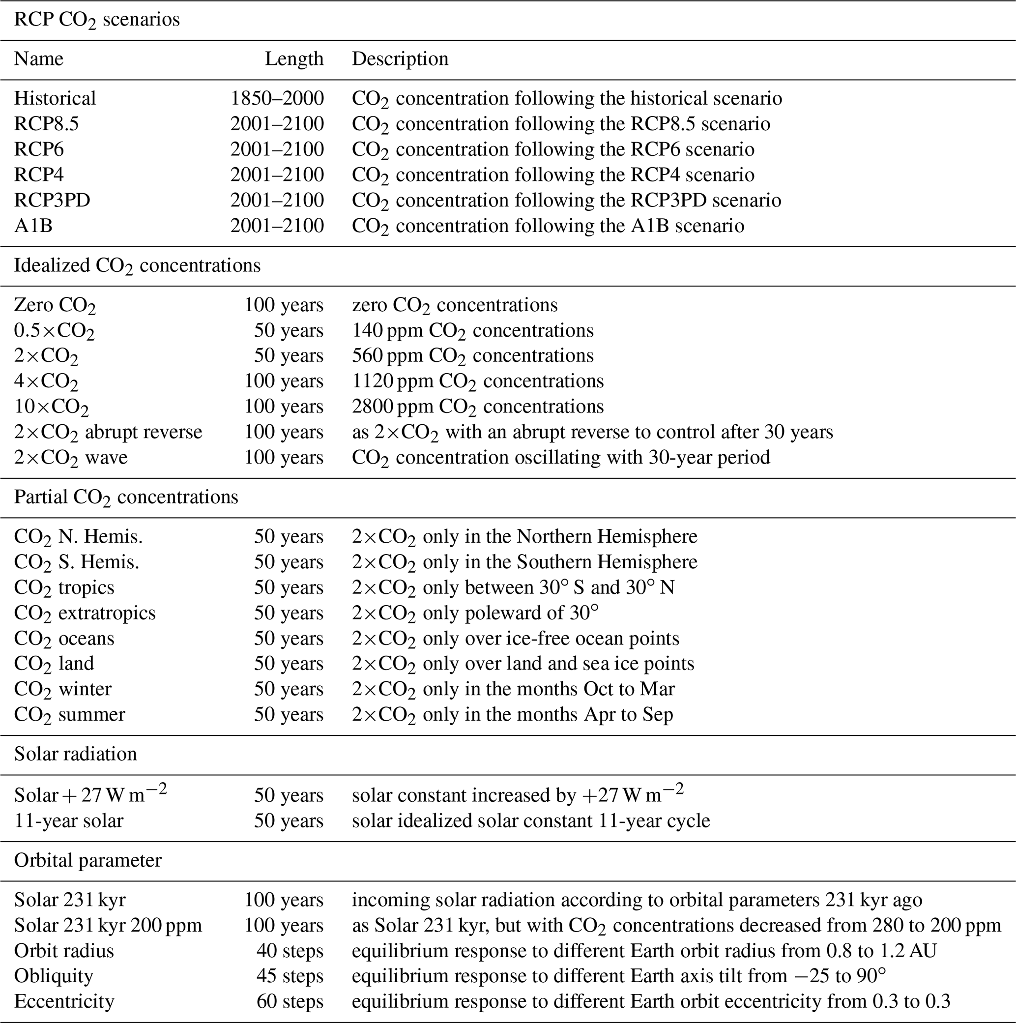
There are a number of different scenarios for external boundary condition changes in the MSCM experiment database. They include different changes in the CO2 concentration and in the incoming solar radiation. A complete overview is given in Table 3. A short description follows below.
2.3.1 RCP scenarios
In the Representative Concentration Pathway (RCP) scenarios the GREB model is forced with time-varying CO2 concentrations. All five different simulations have the same historical time evolution of CO2 concentrations starting from 1850 to 2000, and from 2001 the follow the RCP8.5, RCP6, RCP4.5, RCP2.6, and A1B CO2 concentration pathways until 2100 (van Vuuren et al., 2011).
2.3.2 Idealized CO2 scenarios
The 15 idealized CO2 concentration scenarios in the MSCM experiment database focus on the non-linear time delay and regional differences in the climate response to different CO2 concentrations. These were implemented in five simulations in which the control CO2 concentration (340 ppm) was changed in the first time step to a scaled CO2 concentration of 0, 0.5, 2, 4, and 10 times the control level. The 0.5×CO2 and 2×CO2 simulations are 50 years long and the others are 100 years long.
Two different simulations with idealized time evolutions of CO2 concentrations are conducted to study the time delay of the climate response. In one simulation, the CO2 concentration is doubled in the first time step, held at this level for 30 years, and then returned to control levels instantaneously (2×CO2 abrupt reverse). In the second simulation, the CO2 concentration is varied between the control and 2×CO2 concentrations following a sine function with a period of 30 years, starting at the minimum of the sine function at the control CO2 concentration (2×CO2 wave). Both simulations are 100 years long.
The third set of idealized CO2 concentration scenarios double the CO2 concentrations restricted to different regions or seasons. The eight regions and seasons include the Northern or Southern Hemisphere, the tropics (30∘ S–30∘ N) or extratropics (poleward of 30∘), land or oceans, and the months October to March or April to September. Each experiment is 50 years long.
2.3.3 Solar radiation
Two different experiments with changes in the solar constant were created. In the first experiment, the solar constant is increased by about 2 % (+27 W m−2), which leads to about the same global warming as a doubling of the CO2 concentration (Hansen et al., 1997). In the second experiment, the solar constant oscillates at an amplitude of 1 W m−2 and a period of 11 years, representing an idealized variation of the incoming solar short-wave radiation due to the natural 11-year solar cycle (Willson and Hudson, 1991). Both experiments are 50 years long.
2.3.4 Idealized orbital parameters
A series of five simulations are done in the context of orbital forcings and the related ice age cycles. In one simulation, the incoming solar radiation as a function of latitude and day of the year was changed to its values from 231 kyr ago (Berger and Loutre, 1991; Huybers, 2006). In an additional simulation, the CO2 concentration is reduced from 340 to 200 ppm as observed during the peak of ice age phases in combination with the incoming solar radiation changes. Both simulations are 100 years long.
In three sensitivity experiments, we changed the incoming solar radiation according to some idealized orbital parameter changes to study the effect of the most important orbital parameters. The orbital parameters changed are the distance to the Sun, the Earth axis tilt relative to the Earth–Sun plane (obliquity), and the eccentricity of the Earth orbit around the Sun. The orbit radius was changed from 0.8 to 1.2 AU in steps of 0.01 AU, the obliquity from −25 to 90∘ in steps of 2.5∘, and the eccentricity from 0.3 (Earth closest to the Sun in July) to 0.3 (Earth furthest from the Sun in July) in steps of 0.01. Each sensitivity experiment was started from the control GREB model (1AU radius, 23.5∘ obliquity, and 0.017 eccentricity) and run for 50 years. The last year of each simulation is presented as the estimate for the equilibrium climate.
The MSCM experiment database includes a large set of experiments that address many different aspects of the climate. At the same time, the GREB model has limited complexity and not all aspects of the climate system are simulated in the GREB experiments. The following analysis will give a short overview of some of the results that can be taken from the MSCM experiments. In this we will focus on aspects of general interest and on comparing the outcome to results of other published studies to illustrate the strengths and limitations of the GREB model in this context. The discussion, however, will be incomplete, as there are simply too many aspects that could be discussed in this set of experiments. We will therefore focus on a general introduction and leave space for future studies to address other aspects.
3.1 GREB model performance
The skill of the GREB model is illustrated in Fig. 4 by running the GREB model without the correction terms. For reference, we compare this GREB run with the observed mean climate and seasonal cycle (this is identical to running the GREB model with correction terms) and with a bare world. The latter is the GREB model with all switches OFF (radiative balance without an atmosphere and a dark surface). In comparison with the full GREB model, this illustrates how much all the climate processes affect the climate.
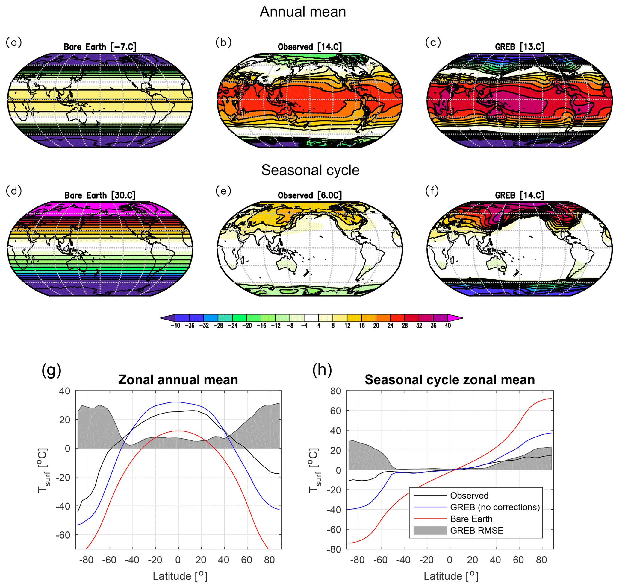
Figure 4Tsurf annual mean (a, b, c) and seasonal cycle (half the difference between mean of July to September minus January to March; d, c, f) for the GREB experiment with all processes turned OFF (bare Earth), only the correction term OFF (GREB), and observed (identical to GREB with all processes ON). The zonal mean of the annual mean (g) and seasonal cycle (h) of the experiments and observations in comparison with the zonal mean RMSE of the GREB model without correction terms relative to observed.
The GREB model without correction terms captures the main features of the zonal mean climate, the seasonal cycle, the land–sea contrast, and even smaller-scale structures within continents or ocean basins (e.g. seasonal cycle structure within Asia or zonal temperature gradients within ocean basins). For most of the globe (<50∘ from the Equator), the GREB model root mean square error (RMSE) for the annual mean Tsurf is less than 10 ∘C relative to the observed (see Fig. 4g). This is larger than for state-of-the-art CMIP-type climate models, which typically have an RMSE of about 2 ∘C (Dommenget, 2012). In particular, the regions near the poles have high RMSE. It seems likely that the meridional heat transport is the main limitation in the GREB model given tropical regions that are too warm, polar regions that are generally too cold, and a seasonal cycle in the polar regions that is too strong in the GREB model without correction terms.
The GREB model performance can be put in perspective by illustrating how much the climate processes simulated in the GREB model contribute to the mean climate relative to the bare world simulation (see Fig. 4). The GREB RMSE to observed is about 20 %–30 % of the RMSE of the bare world simulation (not shown), suggesting that the GREB model has a relative error of about 20 %–30 % in the processes that it simulates or due to processes that it does not simulate (e.g. ocean heat transport).
3.2 Mean climate deconstruction
Understanding what is causing the mean observed climate with its regional and seasonal difference is often central to understanding climate variability and change. For instance, the seasonal cycle is often considered as a first-guess estimate for climate sensitivity (Knutti et al., 2006). In the following analysis, we will give a short overview of how the 10 processes of the MSCM experiments contribute to the mean climate and its seasonal cycle. For these experiments, we use the GREB model without flux correction terms.
In the discussion of the experiments, it is important to consider the fact that climate feedbacks are contributing to the interactions of climate processes. The effect of a climate process on the climate is a result of all the other active climate processes responding to the changes that the climate process under consideration introduces. It also depends on the mean background climate. Therefore, the particular combination of switches with which GREB model experiments are discussed does matter. For instance, the effect of ice–snow cover is stronger in a much colder background climate, but it is also affected by feedback in other climate processes, such as the water vapour feedback. We will therefore consider different experiments or different experiment sets to shed some light on these interactions.
In Figs. 5 and 6 the contributions of each of the 10 processes (except the atmosphere) to the annual mean climate (Fig. 5) and its seasonal cycle (Fig. 6) are shown. In each experiment, all processes are active, but the process of interest and the model correction terms are turned OFF. The results are compared against the complete GREB model without the model correction terms (all processes active; expect model correction terms). For the hydrological cycle we will discuss some additional experiments in which the ice–albedo feedback is turned OFF as well.

Figure 5Changes in the annual mean Tsurf in the GREB model simulations with different processes turned OFF as described in Sect. 2a relative to the complete GREB model without model correction terms: (a) ice–snow, (b) clouds, (c) oceans, (d) heat advection, (e) heat diffusion, (f) CO2 concentration, (g) hydrological cycle, (h) diffusion of water vapour, and (i) advection of water vapour. Global mean differences are shown in the headings. Differences are for the control minus the sensitivity experiment (positive indicates the control experiment is warmer). All values are in degrees Celsius (∘C). In some panels, the values are scaled for better comparison: (b), (c), and (f) by a factor of 2; (a), (d), and (e) by a factor of 3; and (h) and (i) by a factor of 6.
The ice–snow cover (Fig. 5a) has a strong cooling effect, mostly at high latitudes in the cold season, which is due to the ice–albedo feedback. However, in the warm season (not shown) the insulation effect of the sea ice actually leads to warming, as the ocean cannot cool down as much during winter as it does without sea ice.
The cloud cover in the GREB model is only considered as a given boundary condition but does not simulate the formation of clouds. Therefore, it does not include cloud feedbacks. However, mean cloud cover influences the radiation balance of solar and thermal radiation and therefore affects the mean climate and its seasonal cycle. Figure 5b illustrates the fact that cloud cover has a large net cooling effect globally due to the solar radiation reflection effect dominating over the thermal radiation warming effect. Previous studies on the cloud cover effect on the overall climate mostly focus on radiative forcings estimates, but to our best knowledge, they do not discuss how much the mean surface temperature is affected by the mean cloud cover (e.g. Rossow and Zhang, 1995).
It is interesting to note that the strongest cooling effect of cloud cover is over regions with fairly little cloud cover (e.g. deserts and mountain regions). Here it is important to point out that the climate system response to any external forcing or changes in the boundary conditions, such as CO2 forcing or removing the cloud cover, is dominated by internal positive feedback rather than the direct local forcing effect (e.g. see the discussion of the global warming pattern in DF11).
The most important internal positive feedback is the water vapour feedback, which amplifies the effect of removing the cloud cover. This feedback is stronger over dry and cold regions (DF11) and therefore amplifies the effects of removing the cloud cover over deserts and mountain regions.
The large ocean heat capacity slows down the seasonal cycle (Fig. 6c). Subsequently, the seasons are more moderate than they would be without the ocean transferring heat from warm to cold seasons. This is, in particular, important in the middle and higher latitudes. The effect of the ocean heat capacity, however, also has an annual mean warming effect (Fig. 5c). This is due to the non-linear thermal radiation cooling. The non-linear black-body negative radiation feedback is stronger for warmer temperatures, which are not reached in a moderated seasonal cycle with the larger ocean heat capacity. Studies with more complex climate models find similar impacts of the ocean heat capacity on the annual mean and seasonal cycle (e.g. Donohoe et al., 2014).
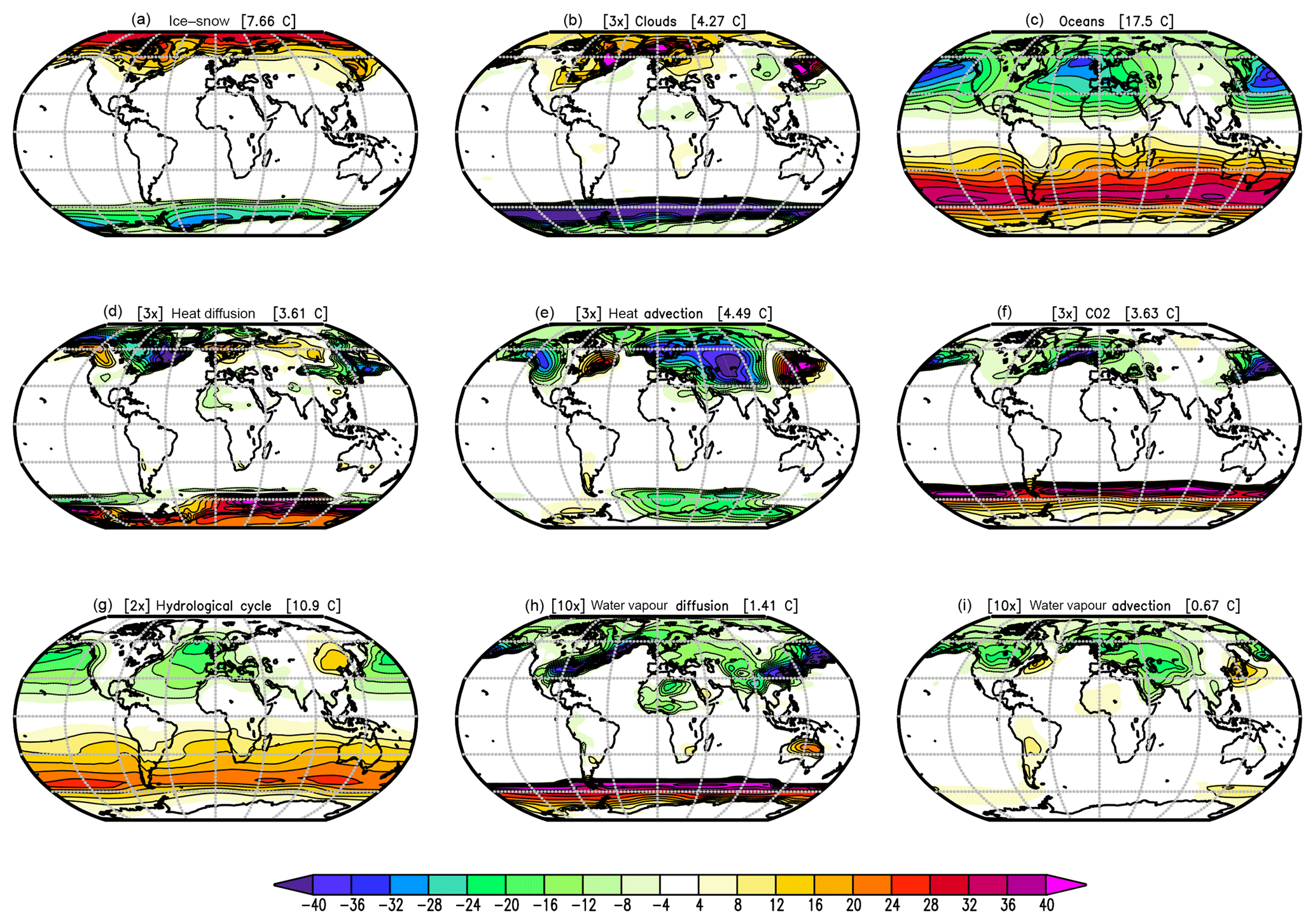
Figure 6As in Fig. 5, but for the seasonal cycle. The mean seasonal cycle is defined by the difference between the months (JAS – JFM) divided by two. Positive values on the Northern Hemisphere indicate a stronger seasonal cycle in the sensitivity experiments than in the full GREB model and vice versa for the Southern Hemisphere. Global root mean square differences are shown in the headings. All values are in degrees Celsius (∘C). In some panels, the values are scaled for better comparison: (b), (d), and (e) by a factor of 2; and (h) and (i) by a factor of 10. (g) The mean for the hydrological cycle experiments with and without the ice–albedo process active.
The diffusion of heat reduces temperature extremes (Fig. 5d). It therefore warms extremely cold regions (e.g. polar regions) and cools the hottest regions (e.g. warm deserts). In global averages, this is mostly cancelled out. The advection of heat has strong effects where the mean winds blow across strong temperature gradients. This is mostly present in the Northern Hemisphere (Fig. 5e). The most prominent feature is the strong warming of the northern European and Asian continents in the cold season. On global average, warming and cooling mostly cancel each other out.
Literature discussions of heat transport are usually based on heat budget analysis of the climate system (in observations or simulations) instead of “switching off” the heat transport in fully complex climate models, since such experiments are difficult to conduct. A similar heat budget analysis of the GREB model experiments is beyond the scope of this study, but the results of these experiments appear to be largely consistent with the findings of heat budget analyses. For instance, the regional contributions of diffusion and advection are similar to those found in previous studies (e.g. Peixoto and Oort, 1992; Yang et al., 2015).
The CO2 concentration leads to a global mean warming of about 9 ∘C (Fig. 5f). Even though it is the same CO2 concentration everywhere, the warming effect is different at different locations. This is discussed in more detail in DF11 and in Sect. 3c.
The input of water vapour into the atmosphere by the hydrological cycle leads to a substantial amount of warming globally (Fig. 5g). However, we need to consider the fact that the experiment with switching OFF the hydrological cycle is the only experiment in which we have a significant amount of global cooling (by about −44 ∘C). As a result, most of the Earth is below freezing temperatures and therefore has a much stronger ice–albedo feedback than in any other experiment. This leads to a significant amplification of the response.
It is instructive to repeat the experiments with the ice–albedo feedback switched OFF (see Supplement Fig. S1). In these experiments, all processes show a reduced impact on the annual mean temperatures, but the hydrological cycle is most strongly affected by it. The ice–albedo effect almost doubles the hydrological cycle response, while for all other processes the effect is about a 10 % to 40 % increase. In the following discussions, we will therefore consider the hydrological cycle impact with and without ice–albedo feedback. In the average of both responses (Figs. 5g and S1g) the hydrological cycle has a global mean impact of about +34 ∘C, with the strongest amplitudes in the tropics. It is still the strongest of all processes.
Similar to the oceans, the hydrological cycle dampens the seasonal cycle (Fig. 6g), but with a much weaker amplitude. The transport of water vapour away from warm and moist regions (e.g. tropical oceans) to cold and dry regions (e.g. high latitudes and continents) leads to additional warming in the regions that gain water vapour and cooling in those that lose water vapour (Fig. 6h). The effect is similar in both hemispheres. The transport of water vapour along the mean wind directions has stronger effects on the Northern Hemisphere than on the Southern Hemisphere, since the northern hemispheric mean winds have more of a meridional component, which creates advection across water vapour gradients (Fig. 6i). This effect is most pronounced in the cold seasons.
Most processes have a predominately zonal structure. We can therefore take a closer look at the zonal mean climate and seasonal cycle of all processes to get a good representation of the relative importance of each process; see Fig. 7. The annual mean climate is most strongly influenced by the hydrological cycle (here shown as the mean of the response with and without the ice–albedo feedback). The cloud cover has an opposing cooling effect but is weaker than the warming effect of the hydrological cycle. The warming effect by the ocean's heat capacity is similar in scale to that of the CO2 concentration.

Figure 7Zonal mean values of the annual mean (a) and seasonal cycle differences (b) for the experiments as shown in Figs. 5 and 6g. The mean for the hydrological cycle is for the experiments with and without the ice–albedo process active.
An interesting aspect of the climate system is that the Northern Hemisphere is warmer than the southern counterpart (by about 1.5 ∘C; not shown), which may be counterintuitive given the warming effect of the ocean heat capacity (see above discussion; Kang et al., 2015). The GREB model without flux correction also has a warmer Northern Hemisphere than the southern counterpart (by about 0.3 ∘C; not shown), whereas the bare Earth (pure black-body radiation balance; GREB all switches OFF) would have the Northern Hemisphere colder than the southern counterpart (by about −0.6 ∘C; not shown). A number of processes play into this inter-hemispheric contrast, with the most important contribution coming from cross-equatorial heat and moisture advection (see Fig. 7a). This is largely consistent with Kang et al. (2015).
The seasonal cycle is damped most strongly by the ocean's heat capacity and by the hydrological cycle. The latter may seem unexpected but is due to the effect of increased water vapour having a stronger warming effect in the cold seasons, similarly to the greenhouse effect of CO2 concentrations. In turn, ice–snow cover and cloud cover lead to an intensification of the seasonal cycle at higher latitudes. Again, the latter may seem unexpected but is due to interaction with other climate feedbacks such as the water vapour feedback, which also makes the climate more strongly respond to changes in cloud cover in regions where there actually is very little cloud cover (e.g. deserts).
As an alternative way of understanding the role of the different process we can build up the complete climate by introducing one process after the other; see Figs. 8 and 9. We start with the bare Earth (e.g. like our Moon) and then introduce one process after the other. The order in which the processes are introduced is mostly motivated by giving a good representation of each of the 10 processes. However, it can also be interpreted as a build-up of the Earth climate in a somewhat historical way: we assume that initially the Earth was a bare planet and then the atmosphere, ocean, and all other aspects were built up over time.
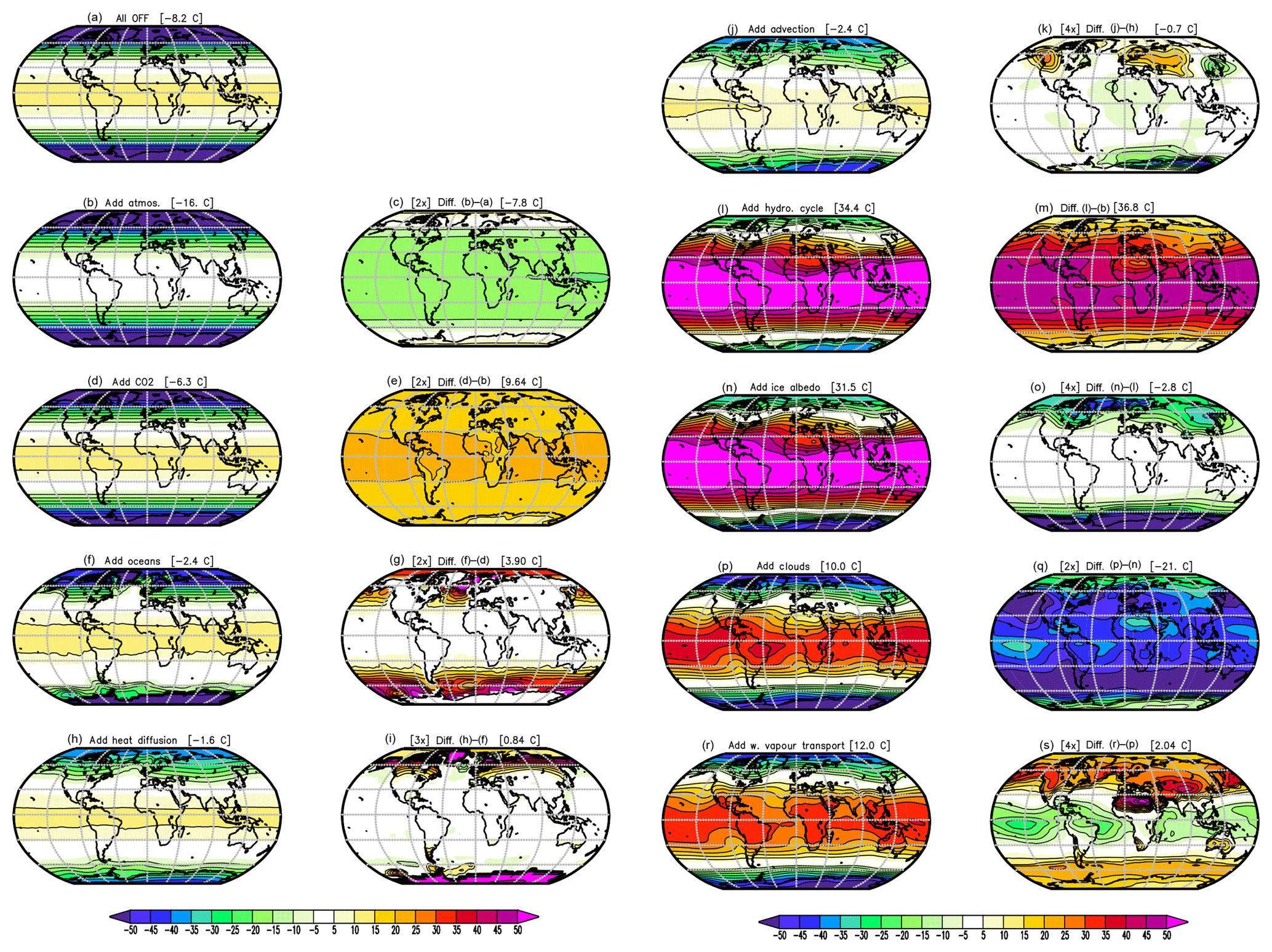
Figure 8Conceptual build-up of the annual mean climate starting with all processes turned OFF (a) and then adding more processes in each row: (b) atmosphere, (d) CO2, (f) oceans, (h) heat diffusion, (j) heat advection, (l) hydrological cycle, (n) ice albedo, (p) clouds, and (r) water vapour transport. Each panel in the second and fourth columns shows the difference between the panel to its left and the preceding panel. Global mean values are shown in the heading. All values are in degrees Celsius (∘C). In some panels the values are scaled for better comparison: (e), (g), and (q) by a factor of 2; (i) by a factor of 3; and (k), (o), and (s) by a factor of 4. For details on the experiments, see Sect. 2a.
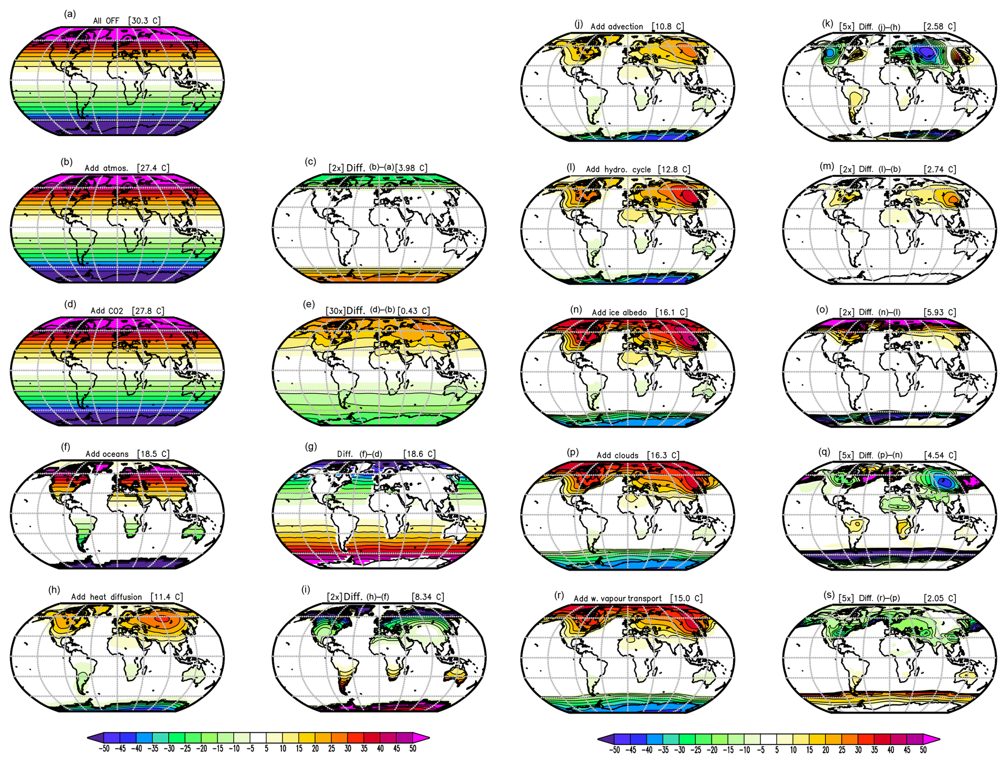
Figure 9As in Fig. 8, but conceptual build-up of the seasonal cycle. The seasonal cycle is defined by the difference between the months (JAS – JFM) divided by two. Global mean absolute values are shown in the heading. In some panels the values are scaled for better comparison: (c), (i), (m), and (o) by a factor of 2; (k), (q), and (s) by a factor of 5; and (e) by a factor of 30.
The bare Earth (all switches OFF) is a planet without atmosphere, ocean, or ice. It has an extremely strong seasonal cycle (Fig. 9a) and is much colder than our current climate (Fig. 8a). It also has no regional structure other than meridional temperature gradients. The combination of all climate processes will create most of the regional and seasonal differences that make up our current climate.
The atmospheric layer in the GREB model simulates two processes if all other processes are turned off: a turbulent sensible heat exchange with the surface and thermal radiation due to residual trace gases other than CO2, water vapour, or clouds. However, as mentioned in Appendix A1 the log-function approximation leads to negative emissivity if all greenhouse gas (CO2 and water vapour) concentrations and cloud cover are zero. The negative emissivity turns the atmospheric layer into a cooling effect, which dominates the impact of the atmosphere in this experiment (Fig. 8b, c). This is a limitation of the GREB model and the result of this experiment as such should be considered with caution. In a more realistic experiment we can set the emissivity of the atmosphere to zero or a very small value (0.01) to simulate the effect of the atmosphere without CO2, water vapour, and cloud cover; see Fig. S2. Both experiments have very similar warming effects in polar regions, suggesting that sensible heat exchange warms the surface. The residual thermal radiation effect from the emissivity of 0.01 has only a minor impact (Fig. S2f and g).
The warming effect of the CO2 concentration is nearly uniform (Fig. 8d, e) and without much of a seasonal cycle (Fig. 9d, e) if all other processes are turned OFF. This accounts for a warming of about +9 ∘C.
The large ocean heat capacity reduces the amplitude of the seasonal cycle (Fig. 9f, g). The effective heat capacity of the oceans is proportional to the observed mixed layer in the GREB model, which causes some small variations (differences from the zonal means) as seen in the seasonal cycle of the oceans. Land points are not affected, since there is no atmospheric transport (advection and diffusion turned OFF). The different heat capacity between oceans and land is already a significant element of the regional and seasonal climate differences (Fig. 8f, g).
Introducing the turbulent diffusion of heat in the atmosphere now enables interaction between points, which has the strongest effects along coastlines and in higher latitudes (Fig. 8h, i). It reduces the land–sea contrast and has strong effects over land with warming in winter and cooling in summer (Fig. 9h, i). The extreme climates of the winter polar region are most strongly affected by turbulent heat exchange with lower latitudes. The turbulent heat exchange makes regional climate differences a bit more realistic.
The advection of heat is strongly dependent on the temperature gradients along the mean wind field directions. It provides substantial heating during the winter season for Europe, Russia, and western North America (Figs. 8j, k, 9j, k). The structure (differences from the zonal mean) created by this process is mostly caused by the prescribed mean wind climatology. In particular, the milder climate in Europe compared to northeast Asia at the same latitudes is created by wind blowing from the ocean onto land. The same is true for the differences between the west and east coasts of northern North America. The climate regional and seasonal structures are now quite realistic, but the overall climate is much too cold. The ice–snow cover further cools the climate, in particular the polar regions (Fig. 8n, o). This difference illustrates the fact that the ice–albedo feedback primarily leads to cooling in higher latitudes and mostly in the winter season.
Introducing the hydrological cycle brings the most important greenhouse gas into the atmosphere: water vapour. This has an enormous warming effect globally (Fig. 8l, m) with a moderate reduction in the strength of the seasonal cycle (Fig. 9l, m). The resulting modelled climate is now much too warm, but introducing cloud cover cools the climate substantially (Fig. 8p, q) and leads to a fairly realistic climate.
The atmospheric transport (diffusion and advection) brings water vapour from relatively moist regions to relatively dry regions (Fig. 8r, s). This leads to enhanced warming in the dry and cold regions (e.g. the Sahara or polar regions) by the water vapour thermal radiation (greenhouse) effect and cooling in the regions where it came from (e.g. tropical oceans). The heating effect is similar to the transport of heat and also has a strong seasonal cycle component.
In the above discussion on how individual climate processes affect the climate we have to keep in mind the limitations of the GREB model and the experimental set-ups. The climate response to changing a single climate element is more complex in the real world than simulated in these GREB experiments. For instance, if the ocean heat capacity is turned OFF it will not just have an effect on the effective heat capacity, but the resulting changes in surface temperature gradients will also affect the atmospheric circulation patterns and subsequently the cloud cover. Such effects on the atmospheric circulation and cloud cover are neglected in the GREB model, as they are given as fixed boundary conditions. Regionally, such effects can be significant and CGCM simulations are required to study such effects.
3.3 2×CO2 response deconstruction
The doubling of the CO2 concentrations leads to a distinct warming pattern with polar amplification, a land–sea contrast, and significant seasonal differences in the warming rate. These structures in the warming pattern reflect complex interactions between feedbacks in the climate system and regional differences in the CO2 forcing pattern. The MSCM 2×CO2 response experiments are designed to help us understand the interactions causing this distinct warming pattern. DF11 discussed many aspects of these experiments with a focus on the land–sea contrast, the seasonal differences, and the polar amplification. We will therefore focus here only on some aspects that have not been previously discussed in DF11.
In the GREB model, we can turn OFF the atmospheric transport and thereby study the local interaction without any lateral interactions. Figure 10 shows three experiments in which the atmospheric transport and other processes (see figure caption) are inactive. The three experiments highlight the regional difference in the CO2 forcing pattern and in the two main feedbacks (water vapour and ice albedo).
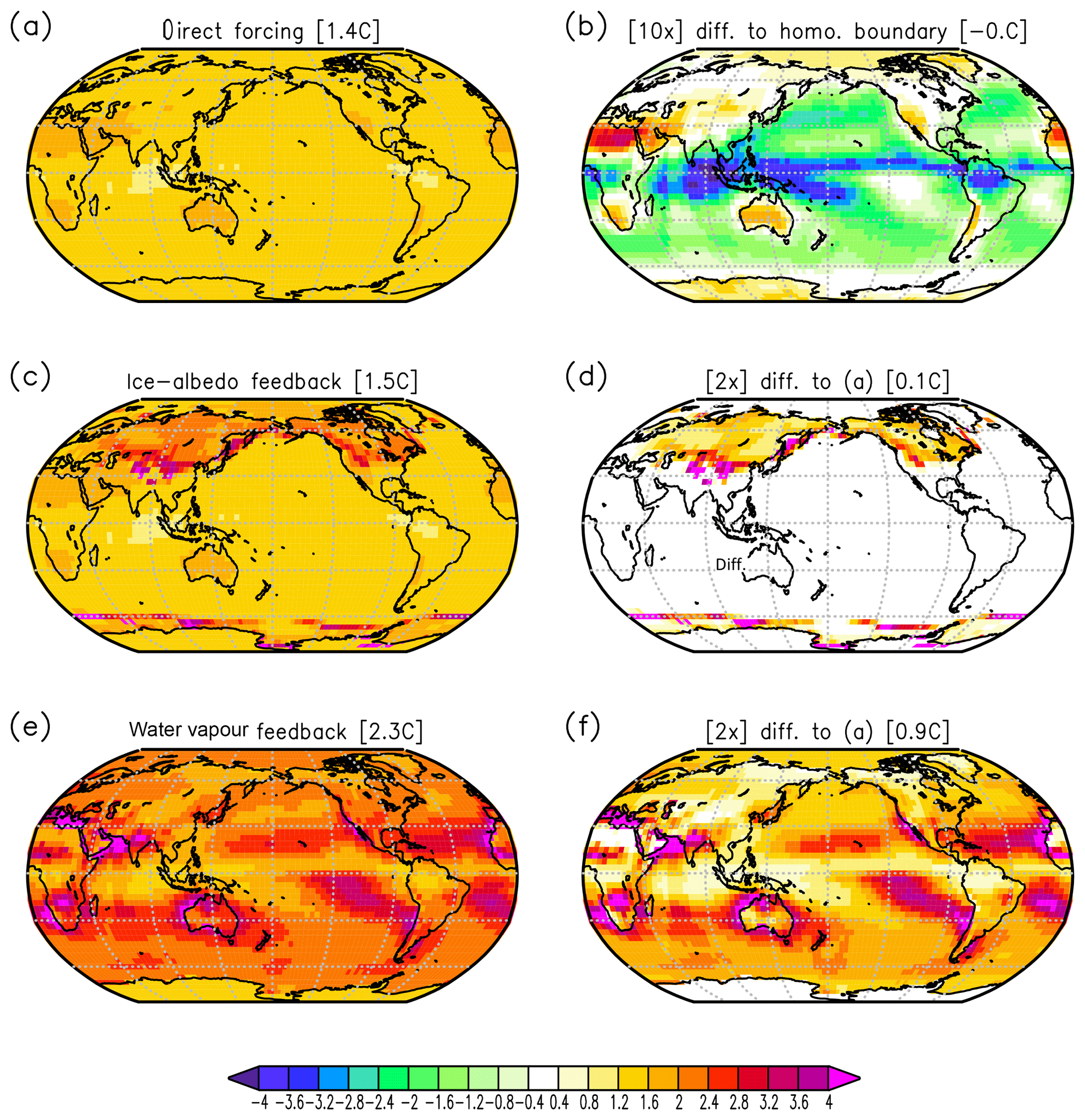
Figure 10Local Tsurf response to doubling of the CO2 concentration in experiments without atmospheric transport (each point on the maps is independent of the others). (a) GREB with topography, humidity, cloud processes, and all other processes OFF. (b) Difference of (a) to GREB with topography and all other processes OFF scaled by a factor of 10. (c) GREB model as in (a), but with the ice–albedo process ON. (d) Difference of (c–a) scaled by a factor of 2. (e) GREB model as in (a), but with hydrological cycle process ON. (f) Difference of (e–a) scaled by a factor of 2. For details on the experiments, see Sect. 2b.
In the first experiment (Fig. 10a) without feedback processes, the local Tsurf response is approximately directly proportional to the local CO2 forcing. The regional differences are caused by differences in cloud cover and atmospheric humidity, since both influence the thermal radiation effect of CO2 (DF11; Kiehl and Ramanathan, 1982; Cess et al., 1993). This causes, on average, the land regions to see a stronger forcing than oceanic regions (see Fig. 10b). However, even over oceans we can see clear differences. For instance, the warm pool of the western tropical Pacific sees less CO2 forcing than the eastern tropical Pacific.
The ice–albedo feedback is strongly localized, and it is strongest over the mid-latitudes of the northern continents and at the sea ice edge around Antarctica (Fig. 10c and d). The water vapour feedback is far more widespread and stronger (Fig. 10e and f). It is strongest in relatively warm and dry regions (e.g. subtropical oceans) but also shows some clear localized features, such as strong Arabian and Mediterranean Sea warming.
3.4 Scenarios
The set of scenario experiments in the MSCM simulations allows us to study the response of the climate system to changes in the external boundary conditions in a number of different ways. In the following, we will briefly illustrate some results from these scenarios and organize the discussion by the different themes in scenario experiments.
The CMIP has defined a number of standard CO2 concentration projection simulations that give different RCP scenarios for future climate change; see Fig. 11a. The GREB model sensitivity in these scenarios is similar to those of the CMIP database (Forster et al., 2013).

Figure 11Global mean Tsurf response to idealized forcing scenarios: (a) different RCP CO2 forcing scenarios. (b) Scaled CO2 concentrations. (c) Idealized CO2 concentration time evolutions (dotted lines) and the respective Tsurf responses (solid lines of the same colour) for the 2×CO2 abrupt reverse (red) and the 2×CO2 wave (blue) simulations. (d) Idealized 11-year solar cycle. The list of experiments is given in Table 3.
Idealized CO2 concentration scenarios help us to understand the response to the CO2 forcing. In Fig. 11b, we show the global mean Tsurf response to different scaling factors of CO2 concentrations. To first order, we can see that the global mean Tsurf response follows a logarithmic CO2 concentration (e.g. any doubling of the CO2 concentration leads to the same global mean Tsurf response; compare 2×CO2 with 4×CO2 or with Fig. 11b) as suggested in other studies (Myhre et al., 1998). However, this relationship does break down if we go to very low CO2 concentrations (e.g. zero CO2 concentration), illustrating the fact that the log-function approximation of the CO2 forcing effect is only valid within a narrow range far away from zero a CO2 concentration.
The transient response time to CO2 forcing can be estimated from idealized CO2 concentration changes; see Fig. 11c. The stepwise change in CO2 concentration illustrates the response time of the global climate. In the GREB model, it takes about 10 years to get 80 % of the response to a CO2 concentration change (see step function response; Fig. 11c). In turn, the response to a CO2 concentration wave time evolution is a lag of about 3 years. The fast versus slow response also leads to different warming patterns with strong land–sea contrasts (not shown) that are largely similar to those found in previous studies (Held et al., 2010).
The regional aspects of the response to a CO2 concentration can also be studied by partially increasing the CO2 concentration in different regions; see Fig. 12. The warming response mostly follows the regions where we partially changed the CO2 concentration, but there are some interesting variations in this. The partial increase in the CO2 concentration over oceans has a stronger warming impact than the partial increase in the CO2 concentration over land for most Southern Hemisphere land regions. In turn, the land forcing has little impact for the ocean regions. The boreal winter forcing has a stronger impact on the Southern Hemisphere than boreal summer forcing, suggesting that the warm season forcing is, in general, more important than the cold season forcing. The only exception to this is the Tibetan Plateau region.
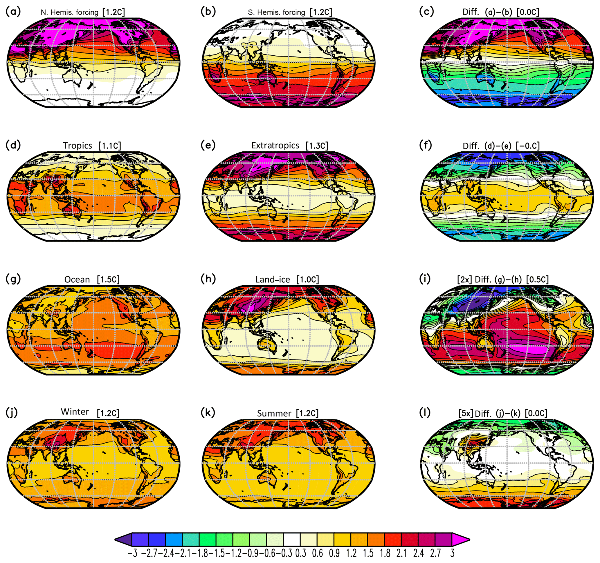
Figure 12Tsurf response to partial doubling of the CO2 concentration in the Northern (a) and Southern (b) Hemisphere, the tropics (d), extratropics (e), oceans (g), land (h), boreal winter (j), and summer (k). The right column shows the difference between the two panels to the left in the same row.
A series of scenarios focus on the impact of solar forcing. In Fig. 11d, we show the response to an idealized 11-year solar cycle. The global mean Tsurf response is 2 orders of magnitude smaller than the response to a doubling of the CO2 concentration, reflecting the weak amplitude of this forcing. This result is largely consistent with the response found in GCM simulations (Cubasch et al., 1997) but does not consider possible more complicated amplification mechanisms (Meehl et al., 2009). A change in the solar constant of +27 W m−2 has a global Tsurf warming response similar to a doubling of the CO2 concentration but with a slightly different warming pattern; see Fig. 13. The warming pattern of a solar constant change has a stronger warming when incoming sunlight is stronger (e.g. tropics or summer season) and a weaker warming in regions with less incoming sunlight (e.g. higher latitudes or winter season). This is in general agreement with other modelling studies (Hansen et al., 1997).
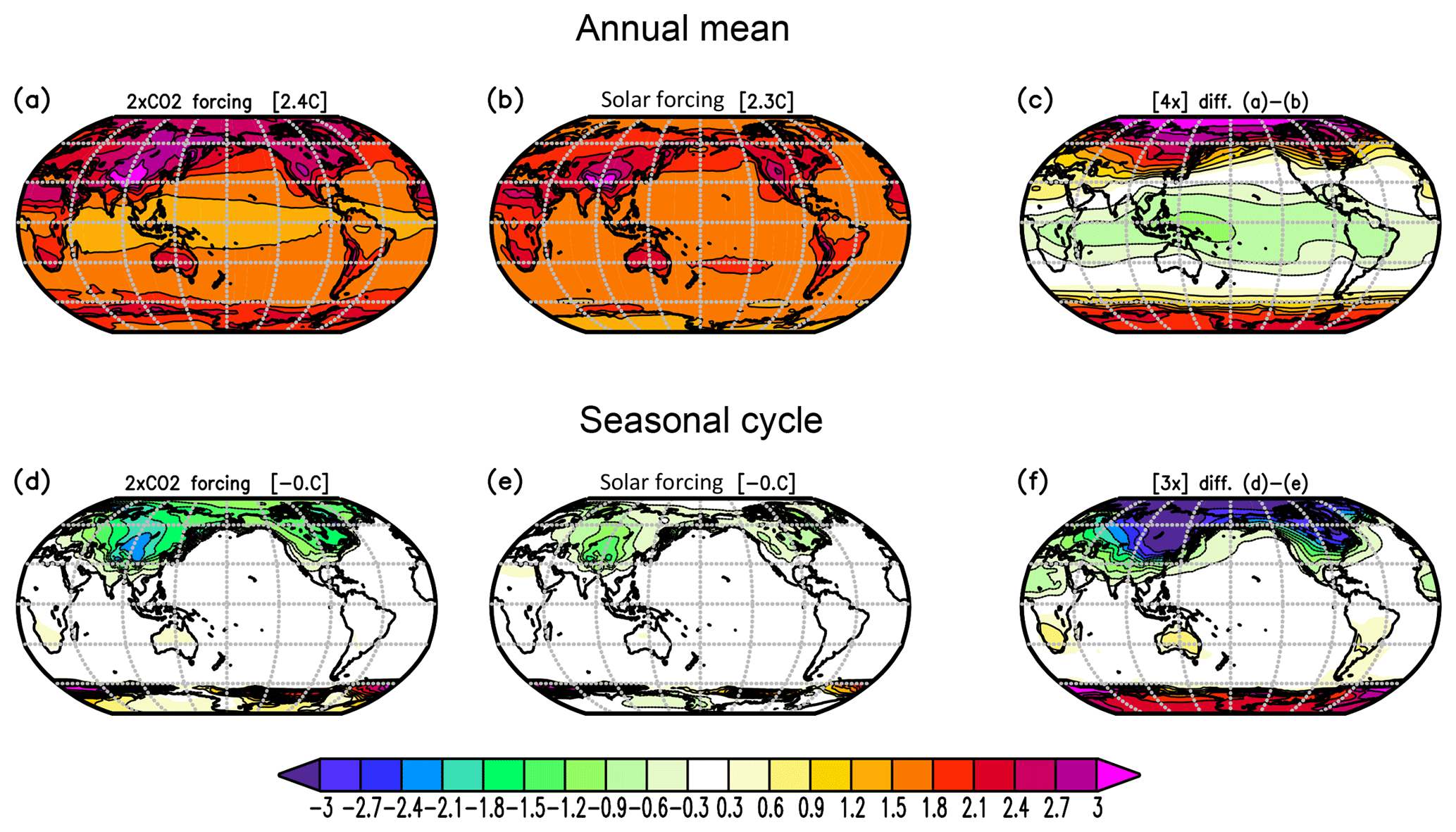
Figure 13Tsurf response to changes in the solar constant by +27 W m−2 (b, e) versus a doubling of the CO2 concentration (a, d) for the annual mean (a, c, c) and the seasonal cycle (d, e, f). The seasonal cycle is defined by the difference between the months (JAS – JFM) divided by two. (c, f) The difference between panels (a) and (b) and between panels (d) and (e), respectively, scaled by 4 (c) and 3 (f).
On longer paleo-timescales (>10 000 years), changes in the orbital parameters affect the incoming sunlight. Figure 14 illustrates the response to a number of orbital solar radiation changes. Incoming radiation (sunlight) typical of the ice age (231 kyr ago) has less incoming sunlight in the northern hemispheric summer. However, it has every little annual global mean change (Fig. 14a) due to increases in sunlight over other regions and seasons. The Tsurf response pattern in the zonal mean in different seasons is very similar to the solar forcing, but the response is slightly more zonal and seasonal differences are less dominant (Fig. 14b). The response is also amplified at higher latitudes. However, in the global mean there is no significant global cooling as observed during ice ages. If the solar forcing is combined with a reduction in the CO2 concentration (from 340 to 200 ppm), we find a global mean cooling of −1.7 ∘C (Fig. 14c), which is still much weaker than observed during ice ages but is largely consistent with previous simulations of ice age conditions (Weaver et al., 1998; Braconnot et al., 2007). This is not unexpected since the GREB model does not include an ice sheet model and, therefore, does not include glacier growth feedbacks that would amplify ice age cycles.
A better understanding of the orbital solar radiation forcing can be gained by analysing the response to idealized orbital parameter changes. We therefore vary the Earth distance to the Sun (radius), the Earth axis tilt to the Earth orbit plane (obliquity), and the shape of the Earth orbit around the Sun (eccentricity) over a wider range; see Fig. 14d–f. When the radius is changed by 10 %, the Earth climate becomes essentially uninhabitable, with either global mean temperature above 30 ∘C (approx. summer mean temperature of the Sahara) or a completely ice-covered snowball Earth. This suggests that the habitable zone of the Earth radius is fairly small due to the positive feedbacks within the climate system simulated in the GREB model (not considering long-term or more complex atmospheric chemistry feedbacks) and largely consistent with previous studies (Kasting et al., 1993).
When the obliquity is zero, the tropics become warmer and the polar regions cool down further than today's climate, as they now receive very little sunlight throughout the whole year. In the extreme case, when the obliquity is 90∘, the tropics become ice covered and cooler than the polar regions, which are now warmer than the tropics today and ice free. The polar regions now have an extreme seasonal cycle (not shown), with sunlight all day during summer and no sunlight during winter. Any eccentricity increase in amplitude would lead to a warmer overall climate. Thus, a perfect-circle orbit around the Sun has, on average, the coldest climate, and all of the more extreme eccentricity (elliptic) orbits have warmer climates. This suggests that the warming effect of the section of the orbit that has a closer transit around the Sun in an eccentricity orbit relative to the perfect-circle orbit overcompensates for the cooling effect of the more remote transit around the Sun in the other half of the orbit relative to the perfect-circle orbit.
In this study, we introduced the MSCM database (version: MSCM-DB v1.0) for research analysis with more than 1300 experiments. It is based on simulations with the GREB model for studies of the processes that contribute to the mean climate, the response to doubling the CO2 concentration, and different scenarios with CO2 or solar radiation forcings. The GREB model is a simple climate model that does not simulate internal weather variability, circulation, or cloud cover changes (feedbacks). It provides a simple and fast null hypothesis for interactions in the climate system and its response to external forcings.
The GREB model without flux corrections simulates the mean observed climate well and has an uncertainty of about 10 ∘C. The model has larger cold biases in the polar regions, indicating that the meridional heat transport is not strong enough. Relative to a bare world without any climate processes the RMSE is reduced to about 20 %–30 % relative to observed. Further, the GREB model emissivity function reaches unphysical negative values when water vapour, CO2, and cloud cover are set to zero. This is a limitation of the log-function parameterization that can potentially be revised if a new parameterization is developed that considers these cases. However, it is beyond the scope of this study to develop such a new parameterization and it is left for future studies.

Figure 14Orbital parameter forcings and Tsurf responses: (a) incoming solar radiation changes in the solar 231 kyr experiment relative to the control GREB model. Tsurf response in solar 231 kyr (b) and solar 231 kyr 200 ppm (c) relative to the control GREB model. Annual mean Tsurf in orbit radius (d), obliquity (e), and eccentricity (f). The solid vertical line in (d–f) marks the control (today) GREB model.
The MSCM experiments for the conceptual deconstruction of the observed mean climate provide a good understanding of the processes that control the annual mean climate and its seasonal cycle. The cloud cover, atmospheric water vapour, and ocean heat capacity are the most important processes that determine the regional difference in the annual mean climate and its seasonal cycle. The observed seasonal cycle is strongly damped not only by the ocean heat capacity, but also by the water vapour feedback. In turn, ice albedo and cloud cover amplify the seasonal cycle in higher latitudes.
The conceptual deconstruction of the response to a doubling of the CO2 concentration based on the MSCM experiments has mostly been discussed in DF11, but some additional results shown here focus on the local forcing in responses without horizontal interaction. It has been shown here that the CO2 forcing has a clear land–sea contrast, supporting the land–sea contrast in the Tsurf response. The water vapour feedback is widespread and most dominant over the subtropical oceans, whereas the ice–albedo feedback is more localized over northern hemispheric continents and around the sea ice border.
The series of scenario simulations with CO2 and solar forcing provide many useful experiments to understand different aspects of the climate response. The RCP and idealized CO2 forcing scenarios give good insights into climate sensitivity, regional differences, transient effects, and the role of CO2 forcing in different seasons or at different locations. The solar forcing experiments illustrate the subtle differences in the warming pattern of CO2 forcing, and the orbital solar forcing experiments illustrated elements of the climate response to long-term paleoclimate forcings.
In summary, the MSCM provides a wide range of experiments for understanding the climate system and its response to external forcings. It builds a basis on which conceptual ideas can be tested to first order, and it provides a null hypothesis for understanding complex climate interactions. Some of the experiments presented here are similar to previously published simulations. In general, the GREB model results agree well with the results of more complex GCM simulations. It is beyond the scope of this study to discuss all aspects of the experiments and their results. This will be left to future studies. Here we need to keep in mind the limitations of the GREB model in not considering atmospheric or ocean circulation changes and not simulating cloud cover feedbacks. Such processes will alter this picture somewhat. The concept of the GREB model may allow researchers to include simple models of atmospheric circulation changes and/or the formation of cloud cover and therefore cloud feedbacks. However, this would require further developments of the GREB to include such processes. Currently, studies of more detailed regional information on future climate change or socio-economic impacts require more complex climate models.
Future development of this MSCM database will continue and it is expected that this database will grow. The development will go in several directions: the GREB model performance in the processes that it currently simulates will be further improved. In particular, the simulation of the hydrological cycle needs to be improved to allow for the use of the GREB model to study changes in precipitation. Simulations of aspects of the large-scale atmospheric circulation, aerosols, carbon cycle, and glaciers would further enhance the GREB model and would provide a wider range of experiments to run for the MSCM database.
The MSCM model code, including all required input files, to do all the experiments described on the MSCM home page and in this paper can be downloaded as a compressed tar archive from the MSCM home page under http://mscm.dkrz.de/download/mscm-web-code.tar.gz (last access: 3 November 2018) or from the bitbucket repository under https://bitbucket.org/tobiasbayr/mscm-web-code (last access: 3 November 2018). The data for all the experiments of the MSCM can be accessed via the MSCM web page interface (DOI: https://doi.org/10.4225/03/5a8cadac8db60; Dommenget, 2018). The mean deconstruction experiment file names have an 11-digit binary code that describes the 11 process switch combinations: 1: ON and 0: OFF. The digits from left to right present the following processes.
-
Model corrections
-
Ice albedo
-
Cloud cover
-
Advection of water vapour
-
Diffusion of water vapour
-
Hydrologic cycle
-
Ocean
-
CO2
-
Advection of heat
-
Diffusion of heat
-
Atmosphere
For example, the data file greb.mean.decon.exp-10111111111.gad is the experiment with all processes ON, but ice albedo is OFF. The 2×CO2 response deconstruction experiment file names have a 10-digit binary code that describes the 10 process switch combinations. The digits from left to right present the following processes.
-
Ocean heat uptake
-
Advection of water vapour
-
Diffusion of water vapour
-
Hydrologic cycle
-
Ice albedo
-
Advection of heat
-
Diffusion of heat
-
Humidity (climatology)
-
Clouds (climatology)
-
Topography (observed)
For example, the data file response.exp-0111111111.2xCO2.gad is the experiment with all processes ON, but ocean heat uptake is OFF. The individual experiments can be chosen from the web page interface by selecting the desired switch combinations. Alternatively, all experiments can be downloaded in a combined tar file from the web page interface.
For all experiments, the datasets include five variables: surface, atmospheric, and subsurface ocean temperature, atmospheric humidity (column-integrated water vapour), and snow–ice cover.
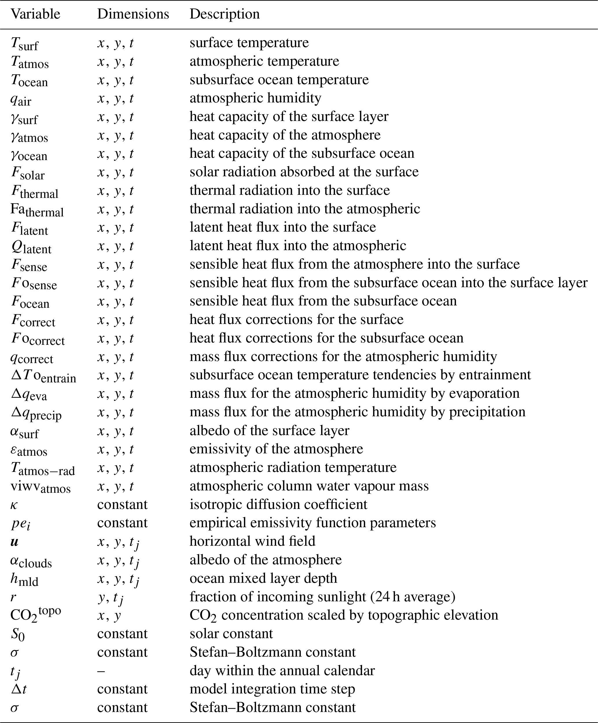
The GREB model has four primary prognostic equations, given below, and all variable names are listed and explained in Table A1. The surface temperature, Tsurf, tendencies are
The atmospheric layer temperature, Tatmos, tendencies are
The subsurface ocean temperature, Tocean, tendencies are
The atmospheric specific humidity, qair, tendencies are
It should be noted here that heat transport is only within the atmospheric layer (Eq. A2). Together with the moisture transport in Eq. (A4) these transports are the only way in which grid points of the GREB model interact with each other in the horizontal directions.
The surface layer heat capacity, γsurf, is constant over land points. For ocean points it follows the ocean mixed layer depth, hmld, if Tsurf is above a temperature range near freezing. Within a range below freezing it is a linear increasing function of Tsurf, and for Tsurf below this range γsurf is the same as over land points (see DF11).
The absorbed solar radiation, Fsolar, is a function of the cloud cover, CLD, boundary condition, and the surface albedo, αsurf:
with the atmospheric albedo, ; αsurf is a global constant if Tsurf is below or above a temperature range near freezing. Within this range it is a linear decreasing function of Tsurf (see DF11). The thermal radiation at the surface is
and the thermal radiation from the atmosphere is
The emissivity of the atmosphere, εatmos, is a function of the cloud cover, CLD, the atmospheric water vapour, viwvatmos, and the CO2 concentration, :
with
The first three terms in Eq. (A9) represent different spectral bands in which the thermal radiation of water vapour and CO2 are active. In the first term both are active, in the second only CO2, and in the third only water vapour. The combined effect of Eqs. (A8) and (A9) is that the sensitivity of the emissivity to CO2 depends on the presence of cloud cover and water vapour.
It is important to note that this log-function parameterization of the emissivity is an approximation developed in DF11 for 2×CO2 concentration experiments. While the parameterization may be a good approximation for a wide range of greenhouse gases, it is likely to have limited skill in extreme variation of greenhouse gases. For instance, if all greenhouse gas (CO2 and water vapour) concentrations and cloud cover are zero, then the emissivity of the atmospheric layer in Eq. (A9) becomes −0.26. This is not a physically meaningful value, and experiments in which all greenhouse gases (CO2 and water vapour) and cloud cover are zero need to be analysed with caution. Section 3.2 (“Mean climate deconstruction”) discusses such limitations in these experiments.
The supplement related to this article is available online at: https://doi.org/10.5194/gmd-12-2155-2019-supplement.
DD contributed to all parts of the study. KN contributed to the development of the web page interface. TB contributed to all parts of the study. DK contributed the design of the model experiments and web page interfaces. CS contributed to all parts of the study. MR contributed to the design of the numerical simulations.
The authors declare that they have no conflict of interest.
This study was supported by the ARC Centre of Excellence for Climate Extremes (CE170100023) and the ARC Centre of Excellence for Climate System Science, Australian Research Council (grant CE110001028). The development of the MSCM web pages was supported by a number of groups (see MSCM web pages). Special thanks go to Martin Schweitzer for his work on the first prototype of the MSCM web pages.
This research has been supported by the Australian Research Council (grant no. CE110001028) and supported by the ARC Centre of Excellence for Climate Extremes (CE170100023).
This paper was edited by Min-Hui Lo and reviewed by two anonymous referees.
Berger, A. and Loutre, M. F.: Insolation Values for the Climate of the Last 10000000 Years, Quaternary Sci. Rev., 10, 297–317, 1991.
Bony, S., Stevens, B., Frierson, D. M. W., Jakob, C., Kageyama, M., Pincus, R., Shepherd, T. G., Sherwood, S. C., Siebesma, A. P., Sobel, A. H., Watanabe, M., and Webb, M. J.: How well do we understand and evaluate climate change feedback processes?, J. Climate, 19, 3445–3482, 2006.
Bony, S., Stevens, B., Frierson, D. M. W., Jakob, C., Kageyama, M., Pincus, R., Shepherd, T. G., Sherwood, S. C., Siebesma, A. P., Sobel, A. H., Watanabe, M., and Webb, M. J.: Clouds, circulation and climate sensitivity, Nat. Geosci., 8, 261–268, 2015.
Boucher, O., Randall, D., Artaxo, P., Bretherton, C., Feingold, G., Forster, P., Kerminen, V.-M., Kondo, Y., Liao, H., Lohmann, U., Rasch, P., Satheesh, S. K., Sherwood, S., Stevens, B., and Zhang, X. Y: Clouds and Aerosols, in: Climate Change 2013: The Physical Science Basis, Contribution of Working Group I to the Fifth Assessment Report of the Intergovernmental Panel on Climate Change, edited by: Stocker, T. F., Qin, D., Plattner, G.-K., Tignor, M., Allen, S. K., Boschung, J., Nauels, A., Xia, Y., Bex, V., and Midgley, P. M., Cambridge University Press, Cambridge, United Kingdom and New York, NY, USA, 2013.
Braconnot, P., Otto-Bliesner, B., Harrison, S., Joussaume, S., Peterchmitt, J.-Y., Abe-Ouchi, A., Crucifix, M., Driesschaert, E., Fichefet, Th., Hewitt, C. D., Kageyama, M., Kitoh, A., Laîné, A., Loutre, M.-F., Marti, O., Merkel, U., Ramstein, G., Valdes, P., Weber, S. L., Yu, Y., and Zhao, Y.: Results of PMIP2 coupled simulations of the Mid-Holocene and Last Glacial Maximum – Part 1: experiments and large-scale features, Clim. Past, 3, 261–277, https://doi.org/10.5194/cp-3-261-2007, 2007.
Cess, R. D., Zhang, M.-H., Potter, G. L., Barker, H. W., Colman, R. A., Dazlich, D. A., Del Genio, A. D., Esch, M., Fraser, J. R., Galin, V., Gates, W. L., Hack, J. J., Ingram, W. J., Kiehl, J. T., Lacis, A. A., Le Treut, H., Li, Z.-X., Liang, X.-Z., Mahfouf, J.-F., McAvaney, B. J., Meleshko, V. P., Morcrette, J.-J., Randal, D. A., Roeckner, E., Royer, J.-F., Sokolov, A. P., Sporyshev, P. V., Taylor, K. E., Wang, W.-C., and Wetherald, R. T.: Uncertainties in Carbon-Dioxide Radiative Forcing in Atmospheric General-Circulation Models, Science, 262, 1252–1255, 1993.
Cubasch, U., Voss, R., Hegerl, G. C., Waszkewitz, J., and Crowley, T. J.: Simulation of the influence of solar radiation variations on the global climate with an ocean-atmosphere general circulation model, Clim. Dynam., 13, 757–767, 1997.
Donohoe, A., Frierson, D. M. W., and Battisti, D. S.: The effect of ocean mixed layer depth on climate in slab ocean aquaplanet experiments, Clim. Dynam., 43, 1041–1055, https://doi.org/10.1007/s00382-013-1843-4, 2014.
Dommenget, D.: Analysis of the Model Climate Sensitivity Spread Forced by Mean Sea Surface Temperature Biases, J. Climate, 25, 7147–7162, 2012.
Dommenget, D. and Floter, J.: Conceptual understanding of climate change with a globally resolved energy balance model, Clim. Dynam., 37, 2143–2165, 2011.
Dommenget, D., Nice, K., Bayr, T., Kasang, D., Stassen, C., and Rezny, M.: Monash Simple Climate Model (webpage interface), https://doi.org/10.4225/03/5a8cadac8db60, 2018.
Forster, P. M., Andrews, T., Good, P., Gregory, J. M., Jackson, L. S., and Zelinka, M.: Evaluating adjusted forcing and model spread for historical and future scenarios in the CMIP5 generation of climate models, J. Geophys. Res.-Atmos., 118, 1139–1150, 2013.
Goosse, H., Brovkin, V., Fichefet, T., Haarsma, R., Huybrechts, P., Jongma, J., Mouchet, A., Selten, F., Barriat, P.-Y., Campin, J.-M., Deleersnijder, E., Driesschaert, E., Goelzer, H., Janssens, I., Loutre, M.-F., Morales Maqueda, M. A., Opsteegh, T., Mathieu, P.-P., Munhoven, G., Pettersson, E. J., Renssen, H., Roche, D. M., Schaeffer, M., Tartinville, B., Timmermann, A., and Weber, S. L.: Description of the Earth system model of intermediate complexity LOVECLIM version 1.2, Geosci. Model Dev., 3, 603–633, https://doi.org/10.5194/gmd-3-603-2010, 2010.
Hansen, J., Sato, M., and Ruedy, R.: Radiative forcing and climate response, J. Geophys. Res.-Atmos., 102, 6831–6864, 1997.
Held, I. M., Winton, M., Takahashi, K., Delworth, T., Zeng, F. R., and Vallis, G. K.: Probing the Fast and Slow Components of Global Warming by Returning Abruptly to Preindustrial Forcing, J. Climate, 23, 2418–2427, 2010.
Huybers, P.: Early Pleistocene glacial cycles and the integrated summer insolation forcing, Science, 313, 508–511, 2006.
Kalnay, E., Kanamitsu, M., Kistler, R., Collins, W., Deaven, D., Gandin, L., Iredell, M., Saha, S., White, G., Woollen, J., Zhu, Y., Chelliah, M., Ebisuzaki, W., Higgins, W., Janowiak, J., Mo, K. C., Ropelewski, C., Wang, J., Leetmaa, A., Reynolds, R., Jenne, R., and Joseph, D.: The NCEP/NCAR 40-year reanalysis project, B. Am. Meteorol. Soc., 77, 437–471, 1996.
Kang, S. M., Seager, R., Frierson, D. M. W., and Liu, X.: Croll revisited: Why is the northern hemisphere warmer than the southern hemisphere?, Clim. Dynam., 44, 1457–1472, https://doi.org/10.1007/s00382-014-2147-z, 2015.
Kasting, J. F., Whitmire, D. P., and Reynolds, R. T.: Habitable Zones around Main-Sequence Stars, Icarus, 101, 108–128, 1993.
Kiehl, J. T. and Ramanathan, V.: Radiative Heating Due to Increased CO2 – the Role of H2O Continuum Absorption in the 12–18 Mu-M Region, J. Atmos. Sci., 39, 2923–2926, 1982.
Knutti, R., Meehl, G. A., Allen, M. R., and Stainforth, D. A.: Constraining climate sensitivity from the seasonal cycle in surface temperature, J. Climate, 19, 4224–4233, 2006.
Lorbacher, K., Dommenget, D., Niiler, P. P., and Kohl, A.: Ocean mixed layer depth: A subsurface proxy of ocean-atmosphere variability, J. Geophys. Res.-Oceans, 111, C07010, https://doi.org/10.1029/2003JC002157, 2006.
Meehl, G. A., Arblaster, J. M., Matthes, K., Sassi, F., and van Loon, H.: Amplifying the Pacific Climate System Response to a Small 11-Year Solar Cycle Forcing, Science, 325, 1114–1118, 2009.
Myhre, G., Highwood, E. J., Shine, K. P., and Stordal, F.: New estimates of radiative forcing due to well mixed greenhouse gases, Geophys. Res. Lett., 25, 2715–2718, 1998.
Peixoto, J. P. and Oort, A. H.: Physics of Climate, Springer US, 1992.
Petoukhov, V., Ganopolski, A., Brovkin, V., Claussen, M., Eliseev, A., Kubatzki, C., and Rahmstorf, S.: CLIMBER-2: a climate system model of intermediate complexity. Part I: model description and performance for present climate, Clim. Dynam., 16, 1–17, 2000.
Roeckner, E., Bäuml, G., Bonaventura, L., Brokopf, R., Esch, M., Giorgetta, M., Hagemann, S., Kirchner, I., Kornblueh, L., Manzini, E., Rhodin, A., Schlese, U., Schulzweida, U., and Tompkins, A.: The atmospheric general circulation model ECHAM 5. Part I: Model description, Reports of the Max-Planck-Institute for Meteorology, 349, 2003.
Rossow, W. B. and Schiffer, R. A.: Isccp Cloud Data Products, B. Am. Meteorol. Soc., 72, 2–20, 1991.
Rossow, W. B. and Zhang, Y. C., 1995: Calculation of Surface and Top of Atmosphere Radiative Fluxes from Physical Quantities Based on Isccp Data Sets.2. Validation and First Results, J. Geophys. Res.-Atmos., 100, 1167–1197, 1995.
Smith, R. S., Gregory, J. M., and Osprey, A.: A description of the FAMOUS (version XDBUA) climate model and control run, Geosci. Model Dev., 1, 53–68, https://doi.org/10.5194/gmd-1-53-2008, 2008.
Taylor, K. E., Stouffer, R. J., and Meehl, G. A.: An Overview of Cmip5 and the Experiment Design, B. Am. Meteorol. Soc., 93, 485–498, 2012.
van Vuuren, D. P., Edmonds, J., Kainuma, M., Riahi, K., Thomson, A., Hibbard, K., Hurtt, G. C., Kram, T., Krey, V., Lamarque, J.-F., Masui, T., Meinshausen, M., Nakicenovic, N., Smith, S. J., and Rose, S. K.: The representative concentration pathways: an overview, Clim. Change, 109, 5–31, 2011.
Weaver, A. J., Eby, M., Augustus, F. F., and Wiebe, E. C.: Simulated influence of carbon dioxide, orbital forcing and ice sheets on the climate of the Last Glacial Maximum, Nature, 394, 847–853, 1998.
Weaver, A. J., Eby, M., Wiebe, E. C., Bitz, C. M., Duffy, P. B., Ewen, T. L., Fanning, A. F., Holland, M. M., MacFadyen, A., Matthews, H. D., Meissner, K. J., Saenko, O., Schmittner, A., Wang, H., and Yoshimori, M.: The UVic Earth System Climate Model: Model description, climatology, and applications to past, present and future climates, Atmos.-Ocean, 39, 361–428, 2001.
Willson, R. C. and Hudson, H. S.: The Suns Luminosity over a Complete Solar-Cycle, Nature, 351, 42–44, 1991.
Yang, H., Li, Q., Wang, K., Sun, Y., and Sun, D.: Decomposing the meridional heat transport in the climate system, Clim. Dynam., 44, 2751–2768, https://doi.org/10.1007/s00382-014-2380-5, 2015.