the Creative Commons Attribution 4.0 License.
the Creative Commons Attribution 4.0 License.
 | 18 Jun 2019
The UKC3 regional coupled environmental prediction system
Huw W. Lewis
Juan Manuel Castillo Sanchez
Alex Arnold
Joachim Fallmann
Andrew Saulter
Jennifer Graham
Mike Bush
John Siddorn
Tamzin Palmer
Adrian Lock
John Edwards
Lucy Bricheno
Alberto Martínez-de la Torre
James Clark
This paper describes an updated configuration of the regional coupled research system, termed UKC3, developed and evaluated under the UK Environmental Prediction collaboration. This represents a further step towards a vision of simulating the numerous interactions and feedbacks between different physical and biogeochemical components of the environment across sky, sea and land using more integrated regional coupled prediction systems at kilometre-scale resolution. The UKC3 coupled system incorporates models of the atmosphere (Met Office Unified Model), land surface with river routing (JULES), shelf-sea ocean (NEMO) and ocean surface waves (WAVEWATCH III®), coupled together using OASIS3-MCT libraries. The major update introduced since the UKC2 configuration is an explicit representation of wave–ocean feedbacks through introduction of wave-to-ocean coupling. Ocean model results demonstrate that wave coupling, in particular representing the wave-modified surface drag, has a small but positive improvement on the agreement between simulated sea surface temperatures and in situ observations, relative to simulations without wave feedbacks. Other incremental developments to the coupled modelling capability introduced since the UKC2 configuration are also detailed.
Coupled regional prediction systems are of interest for applications across a range of timescales, from hours to decades ahead. The first results from four simulation experiments, each of the order of 1 month in duration, are analysed and discussed in the context of characterizing the potential benefits of coupled prediction on forecast skill. Results across atmosphere, ocean and wave components are shown to be stable over time periods of weeks. The coupled approach shows notable improvements in surface temperature, wave state (in near-coastal regions) and wind speed over the sea, whereas the prediction quality of other quantities shows no significant improvement or degradation relative to the equivalent uncoupled control simulations.
- Article
(35411 KB) -
Supplement
(253 KB) - BibTeX
- EndNote


This paper describes the third release of a regional coupled prediction system, termed UKC3, developed to support research to improve the simulation and understanding of the various interactions and feedbacks between different physical and biogeochemical components of the atmosphere, ocean and land across the UK and north-west European shelf region. The UKC3 system represents an incremental update to the second research-mode system, UKC2, described by Lewis et al. (2018). This paper provides a description of the enhancements to model components and of the new coupling science introduced within the latest configuration, and reports on system performance based on new simulations over longer evaluation periods than used to describe the UKC2 performance.
1.1 Motivations for regional coupled model development
Coupled Earth system modelling on global scales, encompassing representation of the physical and biogeochemical feedbacks and interactions between the atmosphere, oceans, cryosphere and land surface, is a well established and mature science discipline, particularly in the context of longer timescale applications from seasonal-range forecasting out to climate change prediction. For applications on shorter timescales or requiring information at more localized scales, including weather forecasting, regional climate scenarios, land management and marine forecasting for example, the discipline of regional coupled prediction has evolved over recent years. This is motivated by a drive from both research and operational applications to develop more wholistic simulations of the environment at high resolution in which the numerous Earth system feedback processes are more explicitly represented (e.g. Shapiro et al., 2010; Pullen et al., 2017a). These systems enable improved understanding of how heat, momentum, freshwater and biogeochemical exchanges affect both marine and atmosphere–land systems.
A number of complex interactions and feedbacks between air, sea and land only become relevant when considering the environment at more localized scales of the order of kilometres. At these scales, for example, mesoscale features such as ocean eddies begin to dominate air–sea interaction processes (e.g. Frenger et al., 2013; Byrne et al., 2015; Oerder et al., 2018), the local landscape and details of precipitation processes become relevant for linking meteorology with catchment-scale hydrology (e.g. Kay et al., 2015; Clark et al., 2016; Kendon et al., 2017), and the influence of freshwater flows on the coastal marine environment become apparent (e.g. Simpson, 1997; Dzwonkowski et al., 2017).
The coastal zone is particularly critical in this context – where the feedbacks between atmosphere, land and ocean state all interplay, and where significant populations live and critically important national infrastructure are sited. The impacts of feedbacks are often manifested through natural hazards, including coastal inundation, flooding and erosion resulting from high waves and storm surge or development of harmful algal blooms and impacts on aquaculture for example. Typically natural hazards from multiple sources may combine or occur concurrently (e.g. Forzieri et al., 2016; Lewis et al., 2015). It is therefore hypothesized that the predictive skill across atmosphere, land hydrology, ocean and wave systems can be improved through explicitly representing the feedbacks between them. Provision of information from coupled systems might also enable an improvement in the range and consistency of actionable information that can be provided through hazard warnings and guidance.
These drivers equally apply on longer timescales, over which the impact of feedbacks on the mean state and extremes may be more significant, and a full Earth system approach may prove to be beneficial for developing relevant regional-scale information of use for planning and policy-making applications (e.g. Miller et al., 2017).
Finally, kilometre-scale regional prediction tools applied in different regions around the world provide a test bed to inform parameterization development in coarser scale systems. As the availability and processing power of high-performance computing increases allowing more routine high-resolution application of global-scale atmosphere (e.g. Jung et al., 2012; Walters et al., 2017), hydrology (e.g. Bierkens et al., 2015; Emerton et al., 2016), ocean (e.g. Hewitt et al., 2017; Holt et al., 2017) and even Earth system (e.g. Palmer, 2012) prediction systems, developing effective coupling mechanisms at the kilometre-scale becomes increasingly relevant.
1.2 Recent progress in regional coupled model research, development and application
The kilometre-scale regional coupled prediction approach is already beginning to reach operational maturity in some forecasting centres and for specific contexts. For example, Durnford et al. (2018) describe the implementation of an integrated water cycle prediction system for the Great Lakes and Saint Lawrence river by Environment Canada, serving a range of applications for industries and populations with exposure to lake water levels. Kunii et al. (2017) and Wada and Kunii (2017) discuss the development of a strongly coupled regional atmosphere–ocean data assimilation system with the Japan Meteorological Agency's configurations, and its potential to improve tropical cyclone prediction through improved representation of the sea surface temperature (SST) initial condition and evolution.
The underpinning research required to improve regional coupled prediction systems, and their application to support process-based research, also continues. This is supported by learning from ongoing development of coupling parameterizations and their application in global-scale coupled systems (e.g. Mogensen et al., 2017; Shimura et al., 2017; Hirons et al., 2018; Donelan, 2018). There is also a critical dependence on the ongoing collection and analysis of relevant air–sea flux measurements in different regions for improving process understanding and supporting model evaluation (e.g. Hackerott et al., 2018; Vinayachandran et al., 2018).
Research using a range of kilometre-scale regional coupled prediction systems continues to deliver new insights. Developing increased understanding and system improvements benefit from the application of a diversity of simulation components and coupling technologies in a range of environments.
For example, Wahle et al. (2017) demonstrated complimentary improvements in both wave and wind forecasts in the complex coastal region of the southern North Sea by implementing wave-induced drag computed by the WAM wave model (Komen et al., 1994) running at 5 km resolution in the COSMO regional atmosphere model (Rockel et al., 2008) run at 10 km resolution. Two-way coupling was achieved using the OASIS3-MCT coupler (Valcke et al., 2015) every 3 min during the simulations. Significant wave height and wind speeds were reduced by approximately 8 % and 3 %, respectively, over a 3-month mean due to the extraction of energy and momentum from the atmosphere by waves. Gronholz et al. (2017) studied the impact of ocean–atmosphere interactions on ocean stratification over a similar model domain. Results demonstrated both the sensitivity of SST to the resolution of atmospheric forcing and that enhanced vertical mixing in the fully coupled ocean simulation during a storm event could have potential impacts for prediction of phytoplankton bloom development. This study applied the Coupled Ocean–Atmosphere–Wave–Sediment Transport (COAWST; Warner et al., 2010) system, based on the WRF (Weather Research & Forecasting; Skamarock and Klemp, 2008) atmosphere model coupled using the Model Coupling Toolkit (MCT; e.g. Larson et al., 2005) to the ROMS (Regional Ocean Modeling System; Shchepetkin and McWilliams, 2005) ocean model, both run at around 10 km horizontal resolution and with a 10 min coupling frequency between components.
Ricchi et al. (2017) also applied the COAWST system to demonstrate the sensitivity of a tropical-like cyclone case study in the Mediterranean Sea (often termed “medicanes”) to coupling. This study also implemented coupling between the atmosphere and ocean to the SWAN (Simulating WAves Nearshore; Booij et al., 1999) wave model. The system was applied at a 5 km horizontal resolution, with model fields exchanged between components every 5 min. While coupling was found to improve the simulation of heat and momentum fluxes for example, it was also highlighted that the sensitivity to details such as the surface roughness parameterization used was greater than the sensitivity to coupling. The beneficial impact of improved SST initial condition and its dynamic evolution through coupling on the simulation of heavy rainfall events in the Mediterranean was discussed by Rainaud et al. (2017), who applied a coupled simulation of the AROME atmosphere (2.5 km resolution) and NEMO ocean (1∕36∘ resolution) models.
Atmosphere–wave coupling over the Mediterranean during a cyclonic event was also assessed by Varlas et al. (2017) applying two-way coupling between WRF atmosphere (10 km resolution) and WAM wave models using the OASIS3-MCT coupler. Coupling was found to impact the evolution of the system, with similar reductions in wind speed and wave height to those discussed by Wahle et al. (2017), and result in an overall improvement of forecast wave height skill by up to 20 % and wind speed by up to 5 % over the sea. This is ultimately anticipated to lead to improved operational warnings and guidance to users.
Recent research focussed on other locations includes the work of Pullen et al. (2017b), who successfully applied a regional coupled model to assess the role of air–sea feedbacks on vortex shedding in the lee of Madeira Island. This modelling system incorporated nested implementations of the NOGAPS atmosphere (Bayler and Lewit, 1992) and NCOM ocean models (Barron et al., 2006), run at up to 2 km horizontal resolution and with coupled fields exchanged every 6 min using the Earth System Modeling Framework (ESMF) coupler through the 20-day simulation period. Seo (2017) used the Scripps Coupled Ocean–Atmosphere Regional model (SCOAR; Seo et al., 2007) over the Arabian Sea, in which WRF and ROMS models were run on 9 km resolution grids and coupled every 6 h. In addition to demonstrating local influences of SST–wind and current–wind interactions in the region, Seo (2017) noted the potential downstream influence and adjustment of the monsoon circulation due to air–sea interaction. Oerder et al. (2018) illustrated the impact of including ocean surface currents in the calculation of atmospheric wind stress, in particular above regions with coherent ocean eddies, in a study region around the eastern Pacific Ocean, Peru and Chile. This research applied a 1∕12∘ resolution implementation of the WRF atmosphere model coupled to a NEMO ocean model on the same horizontal grid, coupled at an hourly frequency using the OASIS3-MCT coupler library. Regional model coupling was also found to improve the simulation of extreme rainfall over Brazil by Luiz do Vale Silva et al. (2018), who applied COAWST at 12 km resolution and found intensification of rain-bearing systems driven by warm SST across the Atlantic Ocean off the coast of Brazil.
A number of other studies continue to examine atmosphere–land–ocean feedback processes in very near-coastal estuarine environments. For example, Marsooli and Lin (2018) applied a two-way coupled ocean–wave prediction system in the New York–New Jersey region for a simulation of Hurricane Sandy to illustrate the benefit of representing coupled feedbacks in an extreme event for improving storm tides. Akan et al. (2017) applied a nested implementation of the COAWST coupled modelling system to examine wave–current interactions at the mouth of the Columbia River. Results show an asymmetric impact of current-induced modification to the wave field, with waves amplified at the mouth of the river due to the impact of tides. The effect of tidal, wind and wave forcing in a near-coastal environment was also highlighted through detailed observations of the Rhine river region of freshwater influence by Flores et al. (2017).
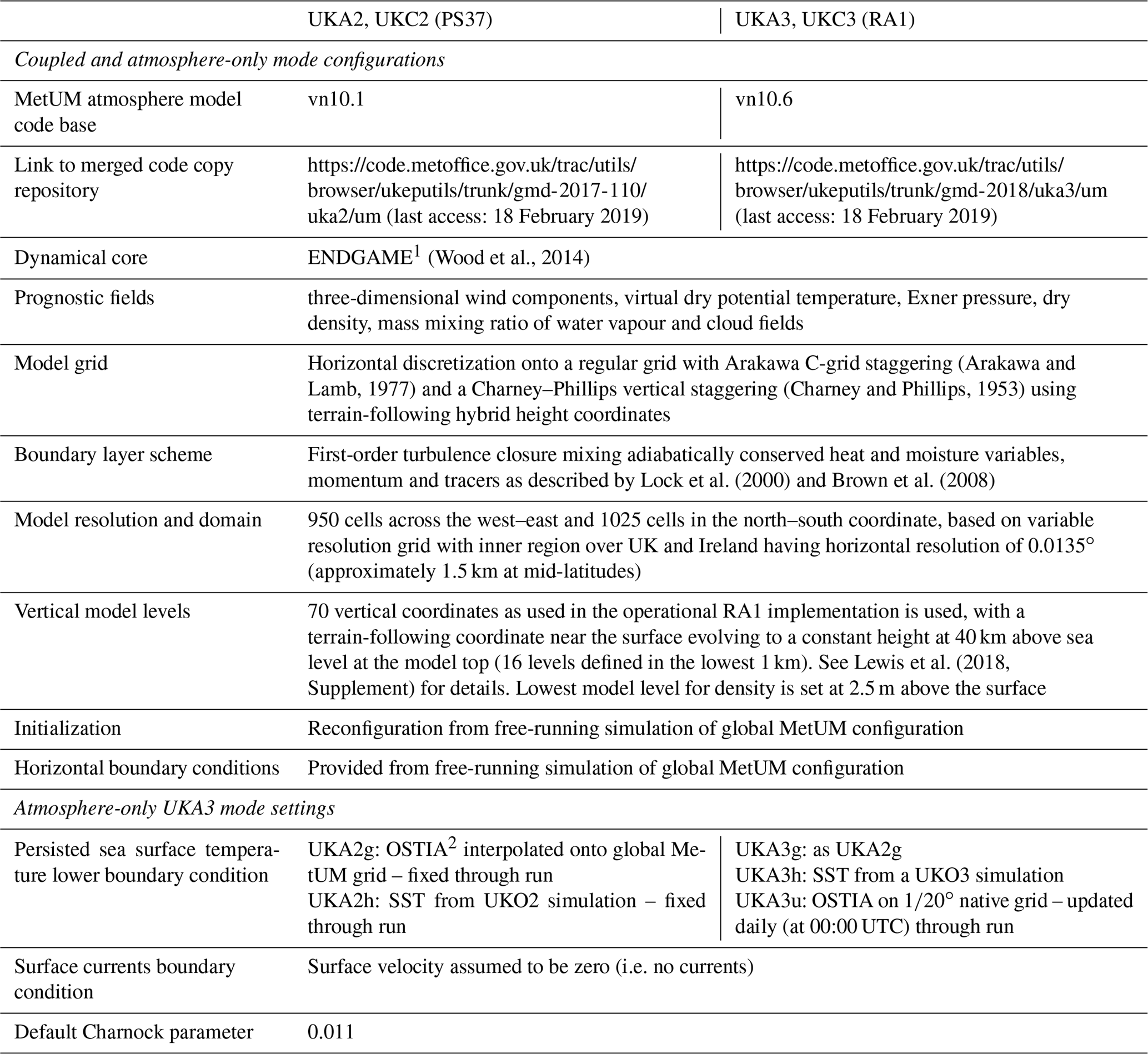
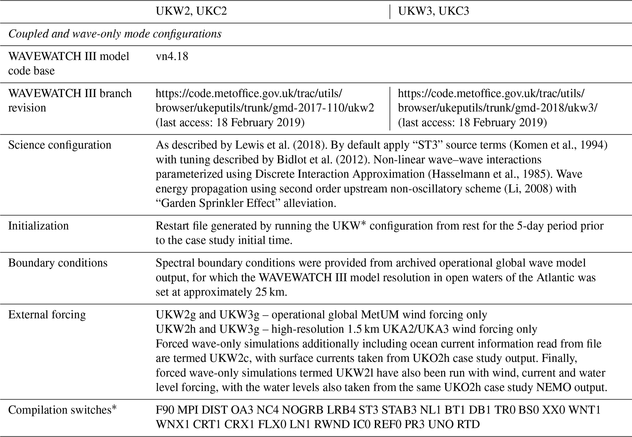
Table 1Summary of key differences and similarities between UKC3 configurations described in this paper and the preceding UKC2 system described by Lewis et al. (2018).
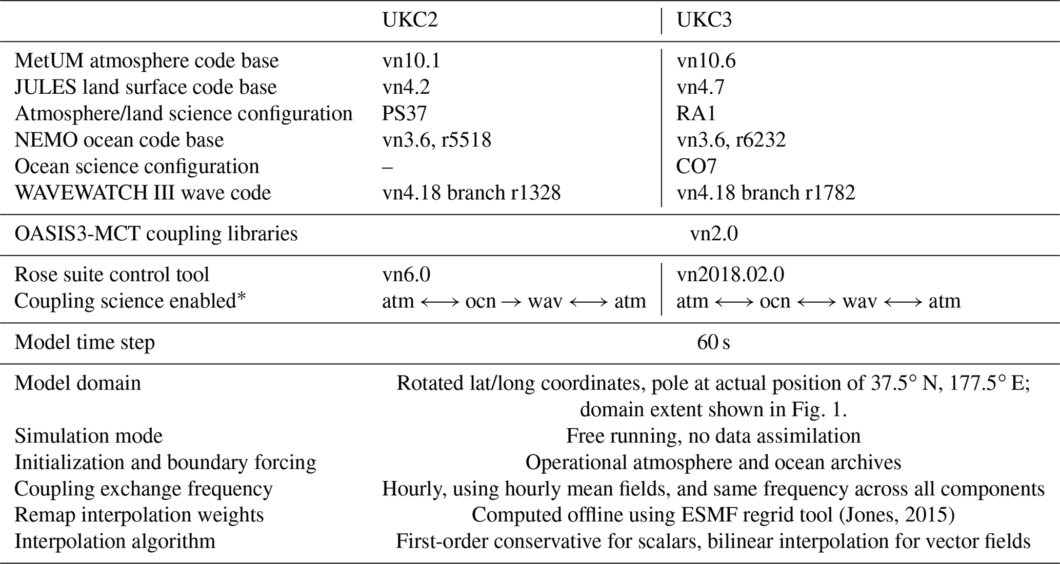
* Note coupling science is described as being enabled between model X and Y in one way as X→Y, or two-way coupling modes as X⟷Y.
1.3 Evolution of the UK and north-west shelf regional coupled system
Lewis et al. (2018) detailed the rationale for developing a regional coupled prediction capability at kilometre-scale resolution for a domain focused on the UK and north-west shelf region, and described the underpinning atmosphere and ocean boundary layer exchanges of momentum and heat, and of the fluxes of freshwater between the atmosphere and land systems before entering the ocean as river discharge. The UKC2 evaluation framework used to run and understand the impact of coupling in case study simulations was also described. This approach and associated naming conventions continues to support the research activities associated with evaluating UKC3 discussed in this paper. Results of the case studies described by Lewis et al. (2018) demonstrated that model performance could be achieved with the UKC2 system that was at least of comparable skill to its component control simulations, with examples where improvements in agreement against in situ observations could be achieved for atmosphere, ocean and wave variables assessed. Further research relevant to the UKC2 system is also described by Fallmann et al. (2017) and Martínez-de la Torre et al. (2018).
A number of limitations and priorities for short- and longer-term future development were also identified by Lewis et al. (2018). The following specific aspects have been addressed within the UKC3 configuration development and are discussed further in this paper.
-
Improving the functionality and flexibility of use for the coupled prediction system (see Sect. 2),
-
Development of wave-to-ocean coupling physics (see Sect. 3),
-
Revisiting a number of assumptions and parameterizations embedded within component models (see Sect. 3),
-
Performing longer simulations, expanding on an initial series of 5-day case studies (see Sect. 4).
This paper is organized as follows. Section 2 introduces the UKC3 regional coupled prediction system, providing details of updates to the UKA3 atmosphere and land, UKO3 ocean and UKW3 wave model configurations since the preceding configurations for each component described by Lewis et al. (2018). Section 3 describes the wave-to-ocean coupling physics introduced within UKC3 configurations. Results from new simulations using the UKC3 configurations during four contrasting month-long experiments are presented in Sect. 4. Conclusions and priorities for future development are discussed in Sect. 5.
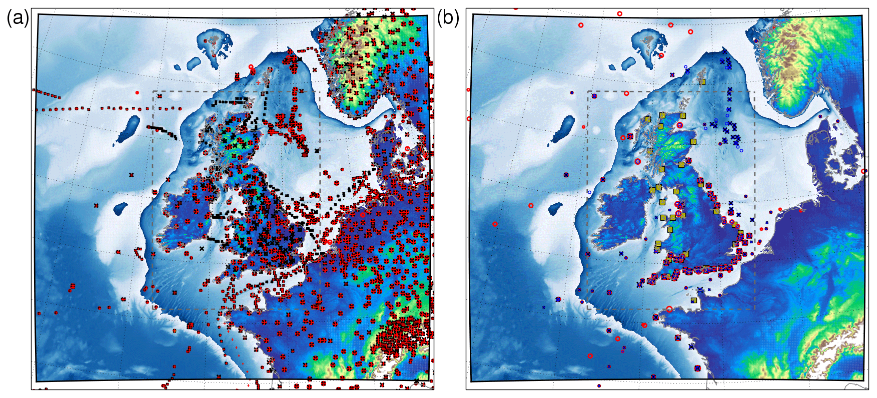
Figure 1Illustration of the UKC3 domain showing the extent of atmosphere/land model domain orography and ocean/wave model domain bathymetry. The regular 1.5 km resolution inner region of the atmosphere model grid is indicated by the dashed grey line. (a) Location of sample of in situ observations on 15 July 2014, relevant for evaluating atmosphere model results. Key to symbols: red circle – visibility, black cross – air temperature and red cross – wind speed and direction. (b) Location of in situ observations on 15 July 2014 relevant for evaluating ocean and wave components. Key: yellow squares – tide gauge sea surface height, red circle – sea surface temperature, black cross – peak wave period and blue circle – significant wave height.
The third release of the regional coupled prediction system UKC3 consists of configurations of the Met Office Unified Model (MetUM) atmosphere (version 10.6; e.g. Brown et al., 2012), and JULES (Joint UK Land Environment Simulator) land surface model (version 4.7; Best et al., 2011; Clark et al., 2011), coupled to the NEMO (Nucleus for European Models of the Ocean) model (version3.6, revision 6232; Madec et al., 2016) and WAVEWATCH III wave model (version4.18; WW3DG, 2016). Coupling is achieved through use of the OASIS3-MCT (Ocean Atmosphere Sea Ice Soil) coupling libraries (version 2.0; Valcke et al., 2015). A naming convention is adopted whereby the atmosphere–land (MetUM–JULES) configuration is termed UKA3, and similarly the uncoupled ocean and wave components as UKO3 and UKW3, respectively.
Table 1 provides a summary of the key differences and similarities between the UKC3 system and the previous UKC2 configuration as described by Lewis et al. (2018). The update of atmosphere, land surface, ocean and wave model codes used in UKC3 in itself represents the addition of new science, inherited from underpinning development of the component model science. Only those aspects where the model codes used in UKC3 have substantially developed between configurations are highlighted in the following sections. The model domain and grid definitions are identical to the UKC2 configuration. The extent of the UKC3 system domain is illustrated in Fig. 1, together with an illustration of the available in situ observing networks used for model evaluation.
Table 2Summary of UKC3 system coupled and uncoupled evaluation suites.
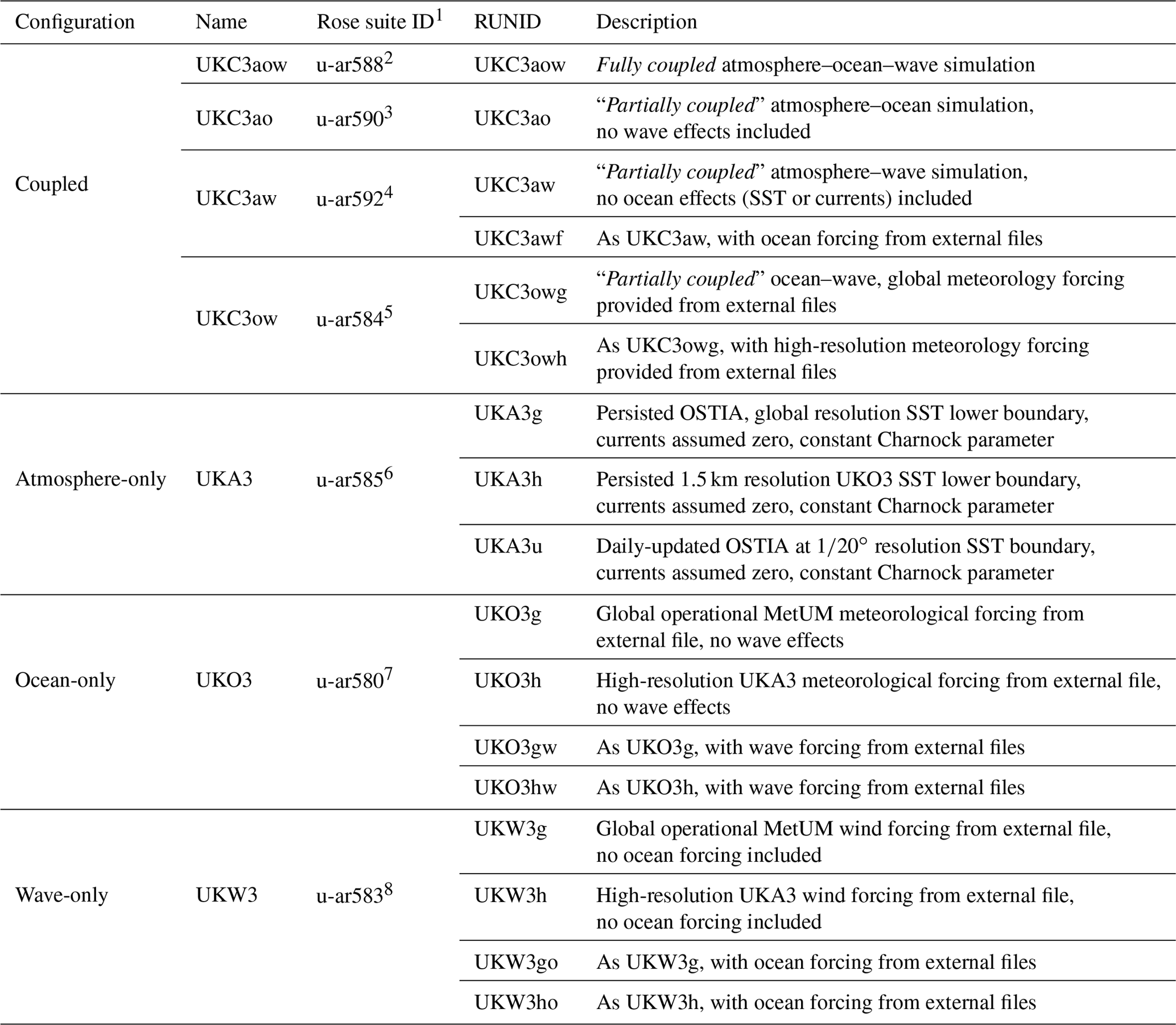
1 All configurations are available to registered researchers
from the https://code.metoffice.gov.uk/trac/roses-u/ (last access:
18 February 2019) repository. The various boundary condition and/or forcing
options described can be enabled
using the RUNID configuration parameter.
2 https://code.metoffice.gov.uk/trac/roses-u/browser/a/r/5/8/8 (last
access: 18 February 2019);
3 https://code.metoffice.gov.uk/trac/roses-u/browser/a/r/5/9/0 (last
access: 18 February 2019);
4 https://code.metoffice.gov.uk/trac/roses-u/browser/a/r/5/9/2 (last
access: 18 February 2019);
5 https://code.metoffice.gov.uk/trac/roses-u/browser/a/r/5/8/4 (last
access: 18 February 2019);
6 https://code.metoffice.gov.uk/trac/roses-u/browser/a/r/5/8/5 (last
access: 18 February 2019);
7 https://code.metoffice.gov.uk/trac/roses-u/browser/a/r/5/8/0 (last
access: 18 February 2019);
8 https://code.metoffice.gov.uk/trac/roses-u/browser/a/r/5/8/3 (last
access: 18 February 2019).
The overall approach to system development and the framework for running simulations as Rose suites is as described by Lewis et al. (2018). Table 2 summarizes the different coupled and uncoupled configurations defined as part of the UKC3 research system. This also introduces the naming convention adopted in order to run the same science and coupling configuration but with different initial conditions or external forcing. Where more than one option is available for a particular configuration, the required configuration can be specified by setting a RUNID environment variable prior to running a simulation.
A number of terms describing each simulation approach are introduced as follows.
-
Fully coupled (UKC3aow): two-way feedbacks represented between all model components within the system.
-
Partially coupled: two-way feedbacks represented between only two components of the system. In the ocean–wave coupled UKC3owg configuration for example, atmospheric forcing is provided from the external operational global MetUM archive, although with wave-modified surface drag coefficient used in the calculation of atmospheric stress from wind components (see Sect. 3.1).
-
Forced mode: information is provided on the state of external components (e.g. the wave state in the ocean model – UKO3gw; or the ocean state in a wave model – UKW3go) as updating surface boundary conditions via file forcing, with no feedbacks represented by the effect of either component on each other. Note that forced mode results are not discussed further in this paper for simplicity.
-
Uncoupled (control): default mode simulations for a given model component, in which no feedbacks with external components are represented. For the UKA3u atmosphere-only control simulations, the SST lower boundary condition is updated with OSTIA data each day and kept constant throughout the day, surface ocean currents are assumed to be zero and a default Charnock parameter constant of 0.011 is assumed. This is in contrast to the UKA3g or UKA3h configurations for which the initial condition SST would persist for the entire duration of a simulation, as applied by Lewis et al. (2018) for 5-day duration case study tests. For the UKO3g ocean-only control simulations, only hourly wind forcing and 3-hourly radiation and moisture fluxes are applied, read as external files from the operational global-scale MetUM archive. For the UKW3g wave-only control simulations, only hourly wind forcing is applied, read as external files from the operational global-scale MetUM archive.
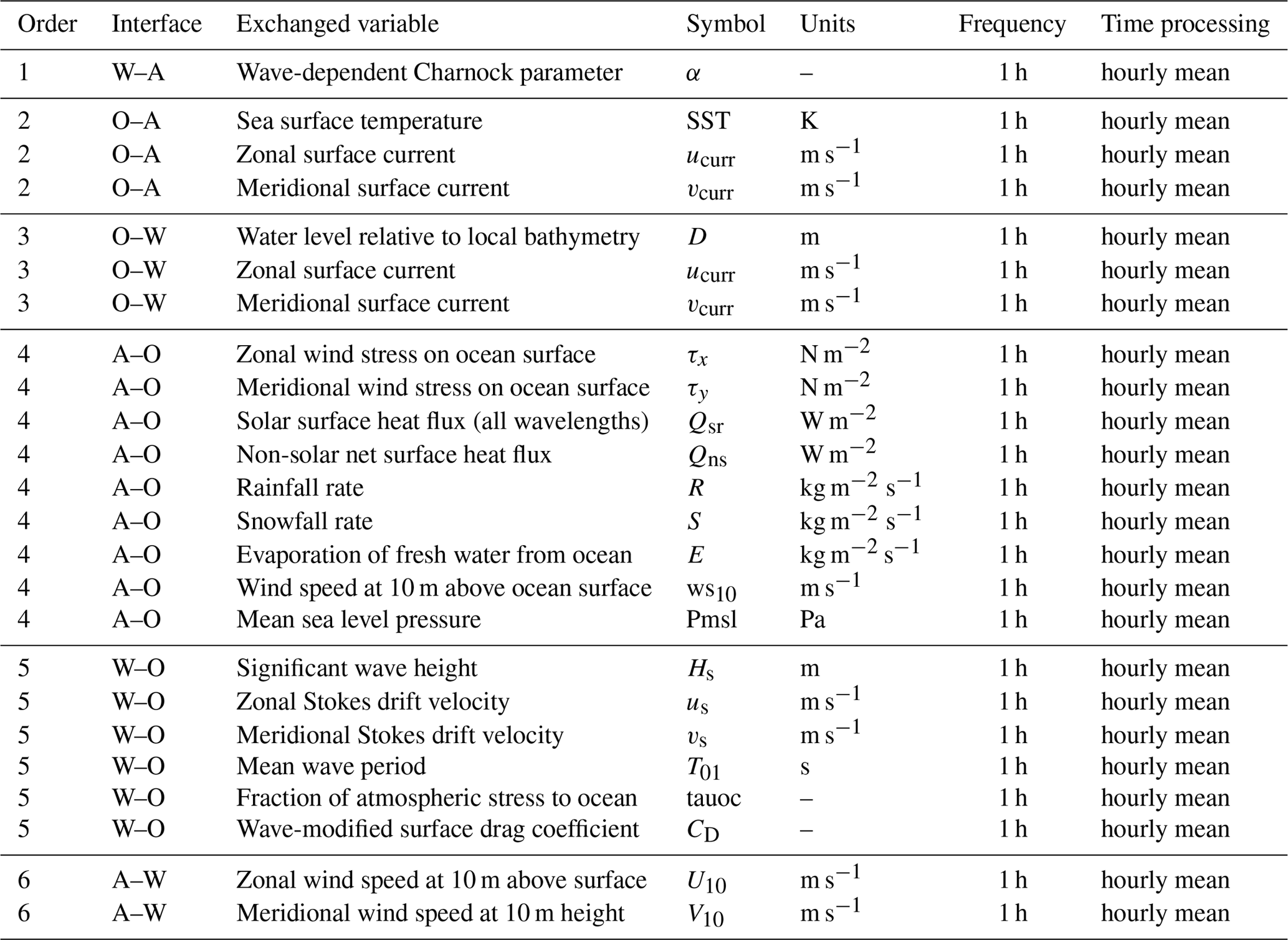
Table 3Summary of coupling exchanges between atmosphere/land (A), ocean (O) and wave (W) components within the UKC3 regional coupled prediction system. Note that the W–O exchanges listed at order 5 are introduced for the first time in UKC3. Other variable coupling is as described by Lewis et al. (2018). Ensuring that exchanges occur between model components in the coupling order shown avoids system deadlocks within OASIS3-MCT. The coupling frequency highlights that all fields are currently exchanged every hour of the simulation time, and that all fields are computed as hourly mean values. See Sect. 2 for further details.
Namelists describing the configuration for all components discussed in this paper are defined as suites under the Rose framework for managing and running model systems (http://metomi.github.io/rose/doc/rose.html, last access: 18 February 2019). All configurations described are made available as Rose suites to registered researchers under a repository at https://code.metoffice.gov.uk/trac/roses-u (last access: 18 February 2019). A more detailed description of the namelists used across all configurations is also included in the Supplement to this paper.
Table 3 lists the coupling exchanges of model variables between each component within UKC3. A total of 24 variables are exchanged, with 6 new exchanges introduced between the WAVEWATCH III wave and NEMO ocean models in UKC3 to support representation of wave-to-ocean feedbacks (discussed further in Sect. 3). Castillo and Lewis (2017) considered a number of aspects related to the optimization and computational costs of the UKC2 system, and assessed that the system runtimes are largely insensitive to the number of fields exchanged between components.
Table 4Summary of UKA3 atmosphere component, and key similarities and differences to the UKA2 configuration described by Lewis et al. (2018).
1 Even Newer Dynamics for General Atmospheric Modelling of the Environment (Wood et al., 2014). 2 Operational Sea Surface Temperature and Sea Ice Analysis (Donlon et al., 2012). Direct links to merged code are provided to support collaboration with registered researchers. Further information on accessing the MetUM can be found at http://www.metoffice.gov.uk/research/collaboration/um-partnership (last access: 18 February 2019).
2.1 The UKA3 atmosphere component
The atmosphere model component within UKC3 (named UKA3 when run in atmosphere-only mode) uses the RA1-M regional atmosphere science configuration described in detail by Bush et al. (2019). This is implemented using the MetUM code at version 10.6 (e.g. Walters et al., 2017). Table 4 highlights the key similarities and differences between UKA3 and UKA2 configurations. Updating between MetUM model code vn10.1 and vn10.6 introduces a substantial number of incremental scientific and technical fixes, enhancements and optimizations, delivered through ongoing model evaluation and development. Technical details on the RA1 science configuration are also provided to registered users of the MetUM code at https://code.metoffice.gov.uk/trac/rmed/wiki/ra1 (last access: 18 February 2019). Key changes introduced between UKA3 (RA1) and the UKA2 (PS37) science configuration in model code or namelist options used of relevance to the regional atmosphere performance are highlighted below. The corresponding namelist changes are listed in Table 5.
Table 5Summary of key changes between UKA2 and UKA3 configuration MetUM namelists, associated with implementing enhanced science options based on regional atmosphere-only model development and evaluation. Registered MetUM users can access further details at https://code.metoffice.gov.uk/trac/rmed/wiki/ra1/protoRA1 (last access: 18 February 2019).
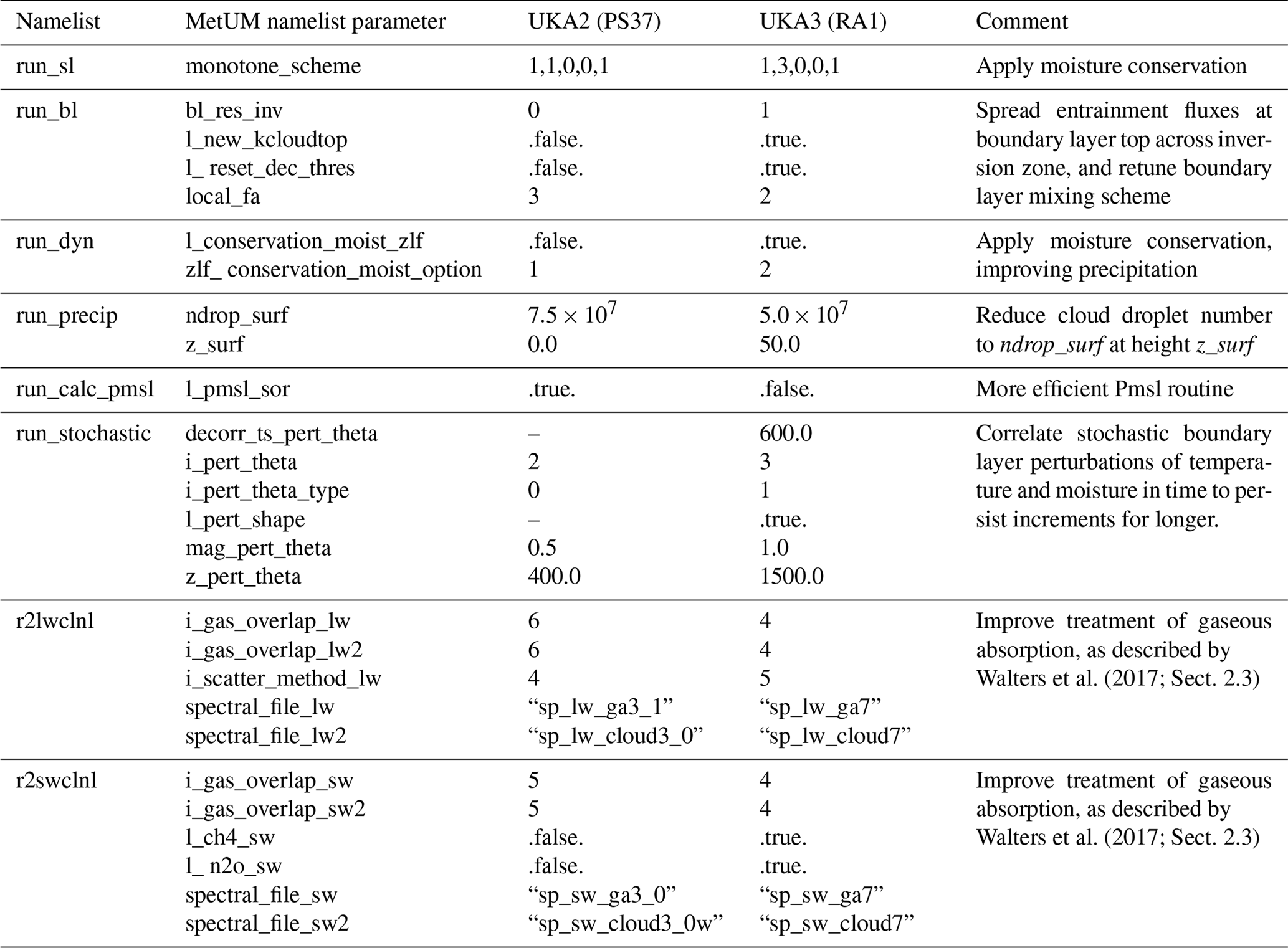
Improvements to simulation of low cloud and fog processes (RA1 ticket no. 1)
Following comparison of 1.5 km resolution model data to field campaign observations (Boutle et al., 2018), changes have been applied to the prescription of cloud droplet number variation with height. Cloud droplet numbers are set to a fixed parameter ndrop_surf below a defined height z_surf above the surface (see Table 5). While based on observations over land, this change is considered important to the evolution of UKC3, relative to UKC2, given evidence that fog and near-surface cloud evolution has been found to be sensitive to air–sea coupling (e.g. Fallmann et al., 2017, 2019).
Improvement to simulation of convective precipitation through moisture conservation (RA1 ticket no. 2)
Long-term application and evaluation of convective-scale configurations of the MetUM (e.g. Clark et al., 2016) have shown that the semi-Lagrangian advection scheme can give rise to spurious sources of moisture, and notably excessive rainfall rates, in the vicinity of resolved convection. The RA1-M configuration introduces global conservation of moisture species following Aranami et al. (2015) (defined by updated run_dyn and run_sl namelist parameters in Table 5). This has a significant beneficial impact on the mean rainfall rates in convective situations, reducing the domain mean accumulations and removing unrealistic extreme precipitation rates (Bush et al., 2019). This improvement is particularly important in the context of fully coupled environmental predictions and a vision of a more integrated representation of the hydrological cycle across atmosphere, land and ocean (e.g. Lewis et al., 2018).
Atmospheric boundary layer simulation enhancements (RA1 tickets nos. 5, 10, 12, 15)
A number of updates have been introduced in the RA1-M science configuration, and thereby in UKA3, related to the atmospheric boundary layer parameterization (run_bl parameters in Table 5). Entrainment fluxes are defined across a diagnosed inversion thickness at the boundary layer top rather than a previously assumed sharp sub-grid layer. Further details on this and other more incremental boundary layer mixing scheme updates are provided by Walters et al. (2017; see discussion of GA7 ticket no. 83) and Bush et al. (2019).
Improved atmospheric absorption and surface radiative fluxes in the MetUM radiation scheme (RA1 ticket no. 9)
The RA1-M science configuration adopts the same treatment of gaseous absorption as used in the GA7 MetUM configuration, described by Walters et al. (2017; see discussion of GA7 ticket no. 16). Briefly, an updated solar spectrum is used for shortwave radiation and improvements are made to the representation of atmospheric composition. These changes result in increased absorption and reduced surface shortwave fluxes in clear-sky conditions. At longwave bands, clear-sky outgoing longwave radiation is reduced and the downwards surface flux increased relative to the UKA2 definition.
Time-correlated stochastic boundary layer perturbations to improve triggering of showers (RA1 ticket no. 25)
The effectiveness of the stochastic boundary layer perturbations, applied in the vicinity of cumulus clouds only, at triggering resolved scale convection has been improved in RA1-M (configured with the run_stochastic namelist options listed in Table 5). Random heating increments can persist for several minutes, and both temperature and moisture perturbations are now applied. Perturbations are based on the surface buoyancy flux, and an option enabled in RA1-M (l_pert_shape = .true.) is also included to weight the perturbations more strongly to the middle of the boundary layer and not at all at the surface. Further details and the implications for precipitation forecasting are discussed by Bush et al. (2019).
Modifications to MetUM for regional atmosphere coupling
As for UKC2, exactly the same codes are compiled and built for both coupled and uncoupled configurations to ensure all simulations are run with identically built code. A number of required code adaptations were implemented as branches to the vn10.6 MetUM trunk code. These are detailed for reference in the Supplement. In general, these modifications can be categorized as being required either to
-
apply the RA1-M graupel definition in the JULES snow scheme (Sect. 2.2),
-
couple effectively between ocean and atmosphere grids with mismatching coastlines, due to grid interpolation of mismatched land/sea masks (as in Lewis et al., 2018),
-
enable dynamic coupling and exchange of information between the atmosphere and a wave model,
-
enable river routing within the coupled MetUM–JULES system,
-
enable consistent coupling of snow when convective snow is explicitly resolved.
To encourage collaboration, a single merged copy of the UKA3 MetUM model code is available to registered researchers via a shared code repository, which can be accessed via https://code.metoffice.gov.uk/trac/utils/browser/ukeputils/trunk/gmd-2018 (last access: 18 February 2019). The code repository location is also linked directly for registered researchers in Table 4.
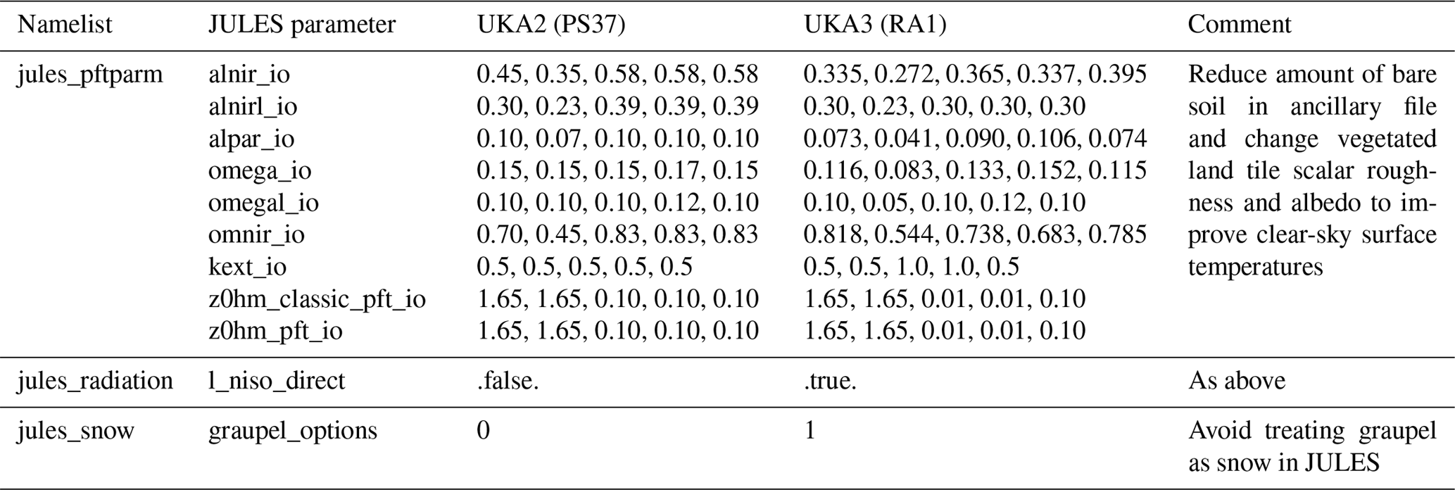
Table 6Summary of UKA3 land surface component, and key similarities and differences to the UKA2 configuration described by Lewis et al. (2018). The direct links to merged code are provided to support collaboration with registered researchers. Further information on accessing JULES can be found at http://jules.jchmr.org (last access: 18 February 2019).

2.2 The UKA3 land surface component
The JULES land surface component within UKC3 is implicitly coupled to the MetUM atmosphere model code, using the method of Best et al. (2004), in all configurations with an atmosphere component. This combined atmosphere–land configuration is termed UKA3. Table 6 lists the key similarities and differences between the land surface specification in UKA3 and UKA2. Details of the trunk code updates between JULES releases vn4.2 and vn4.7 can be accessed at http://jules-lsm.github.io/vn4.7/ (last access: 18 February 2019). The majority of changes, however, are not considered relevant for the regional land surface component. The UKA3 land surface definition is a direct implementation of the RA1-M science configuration, with additional options and parameters enabled for river routing. Key changes introduced in UKA3 are highlighted below, with corresponding namelist changes given in Table 7.
Improved representation of land surface properties to improve near-surface temperature biases (RA1 ticket no. 3)
Four related updates have been implemented in an attempt to reduce clear-sky surface temperature biases over land. These include reducing the amount of bare soil defined and changing the scalar roughness and albedo of vegetated tiles. An updated land use ancillary of land surface tile fractions was generated, using the European Space Agency Climate Change Initiative land cover data set (CCI, 2018) for parts of the domain away from the UK, and taking greater care to account for seasonal variations of the bare soil fraction as a function of the leaf area index (LAI). Further discussion is provided by Walters et al. (2017; see GA7 ticket no. 30) and Bush et al. (2019). Further, scalar roughness length parameters over grass tiles were reduced, by reducing its ratio to the momentum roughness from 0.1 to 0.01 (Table 7). This enhances the difference between surface and air temperatures, in closer agreement with field observational studies. The JULES albedo parameters alnir_io, alpar_io, omega_io and omnir_io were also revised (Table 7).
Ignoring graupel in treatment of JULES snow surfaces (RA1 ticket no. 19)
The JULES namelist parameter graupel_options is set to 1 in RA1-M to avoid the default behaviour of JULES including graupel as snow in the surface scheme when graupel is included in the MetUM surface snowfall diagnostic. While this maintains conservation of water and energy, the properties assigned to new snowfall are considered inappropriate for graupel and this can degrade the surface evolution.
Updated land surface hydrology parameters and runoff generation algorithm
The overall vision and initial implementation for representing the hydrological cycle across UKC2 coupled components was introduced by Lewis et al. (2018). The UKC3 system adopts the same configuration, which is not part of the standard RA1 definition. Martínez-de la Torre et al. (2018) provide a detailed description of the numerous offline tests and conclusions drawn for optimizing the JULES hydrology parameters in order to generate improved runoff characteristics and agreement between river flow simulations and gauge observations.
Modifications to JULES for regional coupling
Similar to the UKC2 system, a number of required code adaptations were implemented as branches to the vn4.7 JULES trunk code to enable regional coupling and run the MetUM–JULES coupled system with river routing. These are detailed for reference in the Supplement. In general, these modifications can be categorized as being required either to
-
apply the RA1 graupel definition in the JULES snow scheme,
-
enable dynamic coupling and exchange of information between the atmosphere and a wave model,
-
apply the Martínez-de la Torre et al. (2018) approach of a slope-dependent Probability Distribution Model runoff generation,
-
enable river routing within the coupled MetUM–JULES system,
-
apply a check in the calculation of surface exchange coefficients for slightly unstable conditions.
A single merged copy of the UKA3 JULES model code is also made available to registered researchers via a shared code repository, which can be accessed via https://code.metoffice.gov.uk/trac/utils/browser/ukeputils/trunk/gmd-2018 (last access: 18 February 2019). The repository location is also linked in Table 7.
Table 7Summary of key changes between UKA2 and UKA3 configuration JULES namelists, associated with implementing enhanced science options based on regional atmosphere-only model development and evaluation. Registered MetUM users can access further details at https://code.metoffice.gov.uk/trac/rmed/wiki/ra1/protoRA1 (last access: 18 February 2019).
2.3 The UKO3 ocean component
The most significant change related to coupling introduced between UKC2 and UKC3 is the implementation and configuration of wave-to-ocean feedbacks within the NEMO ocean model code. Further details are provided in Sect. 3.
Table 8Summary of UKO3 ocean component, and key similarities and differences to the UKO2 configuration described by Lewis et al. (2018). Note that the NEMO compilation key key_harm_ana was only used in UKO3 implementations.
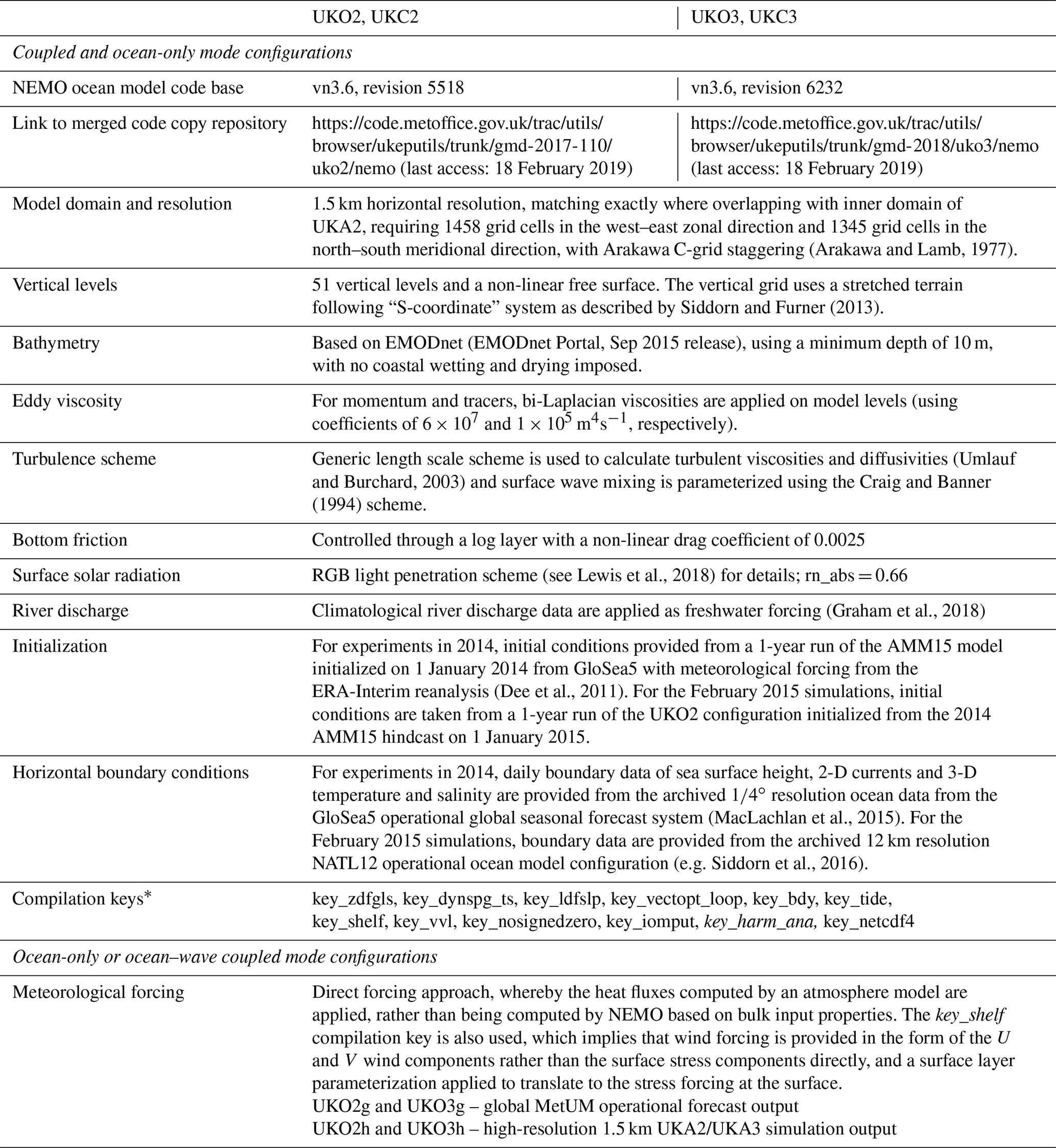
* See the Supplement for description of compilation keys. The direct links to merged code are provided to support collaboration with registered researchers. Further information on accessing NEMO can be accessed at http://www.nemo-ocean.eu (last access: 18 February 2019).
Table 8 highlights other common and differing aspects of the UKO3 regional shelf-seas ocean-only configuration relative to UKO2. Updates were introduced in order to maintain a common science configuration to the evolving Atlantic Margin Model (AMM15) ocean-only shelf-seas forecasting system, which is described in detail by Graham et al. (2018). This required updating the NEMO vn3.6 trunk code revision from r5518 to r6232, which includes a number of minor bug fixes and technical code improvements only. The following configuration changes were also implemented.
Solar radiation penetration and surface restoring parameters
Arnold (2018) describes a number of sensitivity tests conducted using the AMM15 regional ocean model configuration to investigate the impact of different choices in the specification of surface meteorological forcing on simulated SST. Particular consideration was given to the appropriate choice for the ratio of penetrating to non-penetrating shortwave solar radiation in the NEMO “RGB” light penetration scheme (Madec et al., 2016). This study confirms that improved summertime SST were produced when using a rn_abs ratio of 0.66, indicating 66 % absorption at the surface.
Arnold (2018) also highlights the importance of using a surface restoration scheme (ln_ssr = .true., ln_ukmo_haney = .true.) for ocean-only simulations using UKO3. This scheme nudges the simulated SST towards OSTIA, in order to correct for discrepancies between the surface temperatures consistent with the atmospheric forcing and the evolving ocean model climatology. Note that surface restoring was not implemented in UKO2 configurations. It is also not appropriate to apply these corrections when running in ocean–atmosphere coupled mode, given that the atmospheric fluxes are consistent with the underlying ocean model by definition.
Updated Baltic Sea boundary condition
For simplicity in UKO2, the inflow to the domain from the Baltic Sea at the eastern boundary was treated as two river sources, located in the Kattegat Strait. In UKO3, as in AMM15, eastern boundary conditions are instead taken from a regional Baltic simulation (Gräwe et al., 2015). Baltic boundary conditions are applied over a relaxation zone of horizontal width (nn_rimwidth) of 10 grid cells, while boundary conditions into the majority of the domain along the remaining edges are applied over a relaxation zone of 15 grid cells.
Table 9Summary of UKW3 WAVEWATCH III wave model component, highlighting substantive aspects same as for UKW2 configuration described by Lewis et al. (2018).
* A fuller description of the compilation switched is provided in the Supplement. The direct links to merged code are provided to support collaboration with registered researchers. Further information on accessing WAVEWATCH III can be found at http://polar.ncep.noaa.gov/waves/wavewatch (last access: 25 February 2019).
River outflows
Pending further testing and more thorough evaluation of the integrated atmosphere–land system for simulating river flows, by default the river runoff fluxes applied at ocean model coastal grid cells use a climatology as described by Graham et al. (2018), rather than applying the MetUM–JULES calculated flows. The impact of coupling of freshwater between the land and ocean is a priority for future research and development within a subsequent UKC4 system, and will be documented in future publications.
Modifications to NEMO for regional coupling
Section 3 provides a more detailed discussion of the implementation of wave-to-ocean coupling within UKC3, which required a number of code modifications and changes to namelist parameter settings beyond the AMM15 configuration. A single merged copy of the UKO3 NEMO model code has been prepared to be available to registered researchers via a shared code repository, which can be accessed via https://code.metoffice.gov.uk/trac/utils/browser/ukeputils/trunk/gmd-2018 (last access: 18 February 2019). The exact location is linked in Table 8. In general, modifications to the NEMO vn3.6 r6232 trunk code are made to
-
apply capability specific to running NEMO for a domain including a shelf-seas region,
-
implement wave-to-ocean coupling physics,
-
enable NEMO to run within a coupled system without using the MetUM coupling utilities,
-
ensure physically sensible coupled data exchanges in regions of unaligned atmosphere and ocean land/sea masks,
-
when enabled, apply river flux coupling within a sub-domain (UK coastlines only) of the UKC3 domain.
2.4 The UKW3 surface wave component
Table 9 reflects the close similarity in configuration between UKW2 and UKW3 wave model components. This is a result of model code developments being limited to the provision of new coupled fields to support wave-to-ocean coupling (Sect. 3) and some minor bug fixes. A copy of the WAVEWATCH III model code used to define the UKW3 configuration is made available via https://code.metoffice.gov.uk/trac/utils/browser/ukeputils/trunk/gmd-2018 (last access: 18 February 2019) to researchers who are registered as WAVEWATCH III users. The exact path is also linked from Table 9.
A key gap in the UKC2 regional coupled configuration requiring further system development identified by Lewis et al. (2018) was the lack of representation of wave-to-ocean coupling physics. In addition to the feedbacks to the overlying atmosphere through modifying surface roughness, it is well known that surface waves modify momentum exchanges and mixing in the underlying ocean surface boundary layer through a number of different processes. The main interactions represented in the fully coupled atmosphere–ocean–wave UKC3aow system are
- i.
the modification of surface stress by wave growth and dissipation,
- ii.
Stokes–Coriolis force,
- iii.
wave-height-dependent ocean surface roughness.
When forced by an uncoupled atmosphere, the effect of waves in modifying the atmospheric boundary layer can also be accounted for in modifying the calculation of surface stress from wind speed in the NEMO surface forcing. Note that modifications to the NEMO turbulent kinetic energy (TKE) budget due to wave processes are not included in UKC3. Some preliminary tests were conducted exchanging a TKE flux due to breaking waves between the wave and ocean models, but it was considered that further ocean model tuning, related to vertical mixing in particular, would be required before it could be fully implemented. This tuning is an area of ongoing research beyond the scope of the UKC3 configuration.
Breivik et al. (2015) set out the physical basis for the representation of surface wave effects in the NEMO ocean model, as implemented in the global coupled forecast system at the European Centre for Medium-Range Weather Forecasts (ECMWF). Results demonstrate reduced sea surface and sub-surface temperature biases and improvements in the simulated total ocean heat content relative to observations when wave effects are included. On regional scales of relevance to the UKC3 system, a number of previous studies have highlighted the potential importance of representing wave processes for providing improved ocean model simulations. For example, Brown et al. (2011) presented case study evidence of tide–surge–wave interactions from a two-way coupled ocean–wave system based on the POLCOMS (Proudman Oceanographic Laboratory Coastal Ocean Modelling System; Holt and James, 2001) and WAM (Komen et al., 1994) models run at a range of horizontal resolutions at 12 km, 1.8 km and 180 m, focussed on the shallow macrotidal Liverpool Bay region along the north-west English coast during an extreme storm event. Bolaños et al. (2014) extended this work to consider wave–current interactions within the very near coastal zone in the adjacent Dee Estuary. Reza Hashemi et al. (2015) applied the ROMS-SWAN ocean–wave model coupling in the COAWST (Warner et al., 2010) modelling system on a domain across the north-west European shelf of similar extent to that covered by UKC3. Their assessment focussed largely on the impact of ocean tides on the wave model performance, with improvements of up to 25 % in places where wave–current interaction is significant, which is of similar magnitude to that demonstrated by Lewis et al. (2018) from the one-way ocean–wave coupling in UKC2. It is worth noting that both Brown et al. (2011) and Reza Hashemi et al. (2015) commented on the disproportionate increase in computational cost incurred through introduction of the coupled system, relative to production of ocean-only or wave-only results. A summary of UKC3 configuration computational costs are provided in Sect. 4.
Staneva et al. (2016a, b, 2017) describe the application of coupling between wave and ocean models and its impact on improving model performance for the German Bight region of the southern North Sea for several extreme events. A change of 20–30 cm in the forecast surge level was computed in one case when accounting for wave forcing in an ocean model, while wave forcing was found to improve the representation of the vertical ocean profile relative to observations.
The following sections describe wave-to-ocean parameterizations applied in the UKC3 coupled configuration. NEMO parameter settings are highlighted where relevant. A list of all symbols used is provided in Appendix A for reference, and vector quantities are shown in bold-italic.
Appendix B provides a summary of the technical aspects relating to the implementation of wave-to-ocean coupling in the NEMO ocean model and relevant namelist and parameter options. All related ocean model code is now available to the community through an update to the NEMO trunk code resulting from this work (e.g. Law Chune and Aouf, 2018). Researchers and model developers can access this from NEMO vn4.0 (http://nemo-ocean.eu, last access: 18 February 2019).
The branch of the WAVEWATCH III wave model used for UKW3 and UKC3 has also been adapted to support these developments by providing the new coupling functionality, mainly by calculating and/or adding new coupling fields to the coupling communication, and to the diagnostics. The advantage of also adding the new coupling fields to the diagnostics is that the WAVEWATCH III output can be used as input for NEMO working in forcing mode. Careful tests were made to ensure that the models provided the same output when working in forced and coupled modes if the information passed to the models was the same. Comparisons with the WAM wave model code (Komen et al., 1994) have also been made, in particular with relation to the definition of terms in the new wave-modified stress calculations.
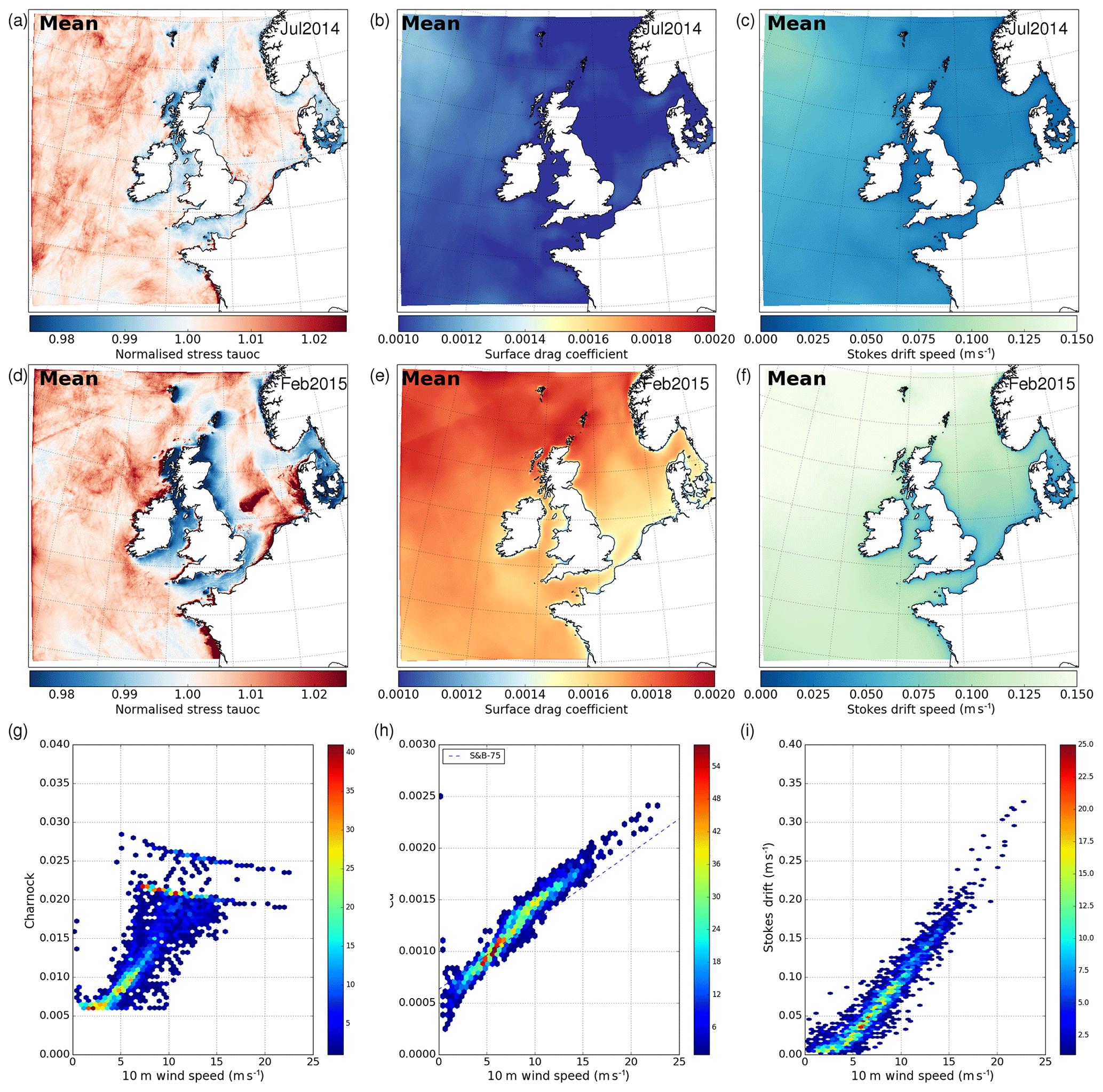
Figure 2Wave model climatology from UKW3g of coupling-related variables – (a, d) normalized stress fraction tauoc, (b, e, h) wave-modified surface drag coefficient and (c, f, i) Stokes drift speed. The maps in (a)–(c) show monthly mean values from the July 2014 “summer” period and in (d–f) from the February 2015 “winter” period. Binned scatter plots on the bottom row show the simulated variation of (g) Charnock parameter, (h) drag coefficient and (i) Stokes drift speed as a function of wind speed across all simulated months in April, July, October 2014 and February 2015 at a point in the central North Sea. Similar distributions are found across the model domain. Colours show the frequency of data within each bin. In (h), the nn_drag = 0 NEMO formulation is plotted by the S&B-75 dashed blue line.
3.1 Momentum modified by drag coefficient (atmospheric forcing modes only)
The wind stress from the atmosphere at the ocean surface that is transmitted to the ocean is modified due to the wave roughness. In a fully coupled system in which the atmospheric boundary layer is modified by the wave state (e.g. UKC3aow), it is considered that this effect is simulated through the wave–atmosphere coupling, and so the ocean component is driven by a wave-modified atmosphere. However, for partially coupled (e.g. UKC3ow) or wave-forced (e.g. UKO3gw) ocean configurations, it is possible to account for the wave-modified drag in computing the wind stress acting on the ocean.
In the UKO3 shelf-sea configuration (with ln_shelf_flx = .true. in namelist namsbc_flx), the wind components are read, and the wind stress is typically calculated from them using a drag coefficient which is a function of the wind velocity (nn_drag = 0) according to Eq. (1; Smith and Banke, 1975). In the new coupled or wave-forced implementation (ln_cdgw = .true.), the shelf sea configuration is also used and the drag coefficient CD is calculated by the wave model (nn_drag = 1), and applied as shown in Eq. (2). This formulation can also be used (nn_drag = 2) with a constant value for CD, set at 0.0015.
Alternative implementations of this effect are also available for use with bulk forcing mode configurations of NEMO.
As highlighted by Eq. (1), CD is a function of wind speed. Figure 2b and e illustrate the distribution of CD computed by the UKW3g WAVEWATCH III wave model configuration for a summer and winter month, and Fig. 2h shows its simulated variation as a function of forcing wind speed at a selected point in the North Sea. This shows values of between approximately 0.005 and 0.0025. The nn_drag = 2 default constant of 0.0015 appears to correspond to forcing winds of approximately 10 m s−1. There is a general tendency for the wave-simulated CD to exceed the default nn_drag = 0 formulation (i.e. Eq. 1; Smith and Banke, 1975) for wind speeds in excess of approximately 5 m s−1, and produce lower values for slower wind speeds. Results from UKC3ow and UKW3go simulations (not shown) also confirm generally low sensitivity of CD values to the presence of ocean forcing or coupling in the wave model.
3.2 Momentum fraction transferred to the ocean through wave breaking
Part of the momentum that the ocean receives from the atmosphere (after taking into account the effect of wave roughness either through wave–atmosphere coupling or modifying the drag coefficient through Sect. 3.1) is stored in surface waves through wave growth or released from the surface waves on wave breaking. The momentum that will actually force the ocean is therefore a fraction of the atmospheric momentum, which is calculated within the wave model according to Eq. (3). The fraction of atmospheric momentum transferred to the ocean is approximated by the normalized momentum flux variable tauoc (Breivik et al., 2015).
The following definitions are used to describe each component of the surface momentum budget.
-
τatm: stress applied by atmosphere on ocean surface
-
τwav: momentum flux absorbed by wave field
-
τwav:ocn: momentum stored by waves released to ocean through wave breaking
-
τocn: water-side stress transmitted into the ocean
Note that, as in Breivik et al. (2015), τwav and τwav:ocn terms are computed from the wave model source terms across the model's frequency range only. This implies that input and dissipation are balanced at higher frequencies. Further work is required to fully account for the tails of the wave frequency range.
Figure 2a and d show the mean simulated tauoc for a summer and winter month, and highlighted values tend to lie in the range 0.95 to 1.05 (i.e. approximately 5 % modification to the atmosphere surface stress due to waves). Largest enhancement can be found along west-facing coastlines, and largest reductions in the lee of land such as downstream of the Scottish islands, in the Irish Sea and along the English Channel. The spatial distribution is broadly consistent between summer and winter months, but with the magnitude of wave modification clearly increased in winter.
3.3 Stokes–Coriolis drift
The Stokes drift, caused by finite amplitude waves, creates a relative motion along the wave direction which quickly decays with depth. The NEMO momentum equation is modified to account for the Stokes drift velocity vs, taking into account the Coriolis forcing, as in Eq. (4).
As only the surface Stokes drift, v0, is usually available from the wave model, different parameterizations are used to estimate the change in the Stokes drift velocity with depth, vs(z), as a function of the mean wave period, t01; significant wave height, Hs; and peak wave frequency ωp. Options are controlled by the nn_sdrift NEMO namelist parameter.
For nn_sdrift = 0, the Breivik 2015 parameterization is used (Breivik et al., 2015, Eq. 120), with the Stokes drift velocity profile vs(z) given by Eq. (5). If nn_sdrift = 1, the Phillips parameterization (Breivik et al., 2016, Eq. 100) is applied using an inverse depth scale, according to Eq. (6). An extension can be applied if nn_sdrift = 2 using the peak wave number as calculated by the wave model rather than the inverse depth scale, as shown in Eq. (7).
Figure 2c, f and i also show a summer and winter spatial distribution of the surface Stokes drift velocity and its variability with wind speed.
3.4 Wave-modified surface roughness
The ocean surface roughness, which has an effect in the vertical mixing by defining the surface turbulent mixing length scale, can be calculated in different ways. In the generic length scale (GLS) turbulent closure scheme, used in the UKO3 configurations; this is dependent on the choice of parameter nn_z0_met. For example, Eqs. (8) and (9) show the simplest approach defining either a constant roughness or constant Charnock parameter via namelist settings.
Rascle et al. (2008) discuss how the roughness length is more physically related to the scale of breaking waves and related eddies responsible for high mixing levels close to the surface, and that it can be related to the significant wave height Hs (or more strictly the wind-sea wave height).
By default in UKO3 ocean-only configurations, the Rascle et al. (2008) parameterization for Hs (nn_z0_met = 2) is used. This estimates the wave age and subsequently significant wave height Hs as a function of wind speed, through Eq. (10a) and (10b).
Here is a typical friction velocity (0.3 m s−1). The surface roughness length z0 is then taken as a fraction rn_frac_hs (default value 1.3) of the estimated Hs. The appropriate value for this factor for the north-west shelf region should be reviewed further before consideration of this scheme for operational applications, while further development might consider the coupling of the wind-sea wave height computed by WAVEWATCH III explicitly.
When using wave forcing or coupling (nn_z0_met = 3), the same approach is used but with the wave model significant wave height replacing the Rascle et al. (2008) estimate, according to Eq. (11).
4.1 Evaluation framework
Lewis et al. (2018) described the development of an evaluation framework to understand the performance of model components run within coupled systems relative to uncoupled approaches. All coupled and uncoupled configurations defined in Table 2 are provided as Rose suites (http://metomi.github.io/rose/doc/rose.html, last access: 18 February 2019) and version controlled under the Flexible Configuration Management (FCM) system (http://metomi.github.io/fcm/doc/, last access: 18 February 2019). A number of different options for initial conditions or forcing are available for each configuration (Table 2), which are enabled within a given suite by setting the relevant RUNID environment variable.
4.2 Model experiments
The focus of UKC3 system evaluation discussed in this paper is on a series of four coupled and forced simulation experiments, each of approximately 1-month duration. This enables assessment across a variety of meteorological conditions within a given month and of ocean and wave results across a spring–neap tidal cycle, and covers evaluation at different times of the year. In order to capture a range of conditions, experiments are conducted for the following periods:
- a.
“Spring”: 30 March–19 April 2014
- b.
“Summer”: 30 June–30 July 2014
- c.
“Autumn”: 30 September–30 October 2014
- d.
“Winter”: 30 January–28 February 2015
This approach extends the analysis of Lewis et al. (2018) who considered a number of relatively short 5-day case study simulations across a range of conditions. By extending the simulation period, it is hoped to provide a more comprehensive evaluation of system performance and to establish whether any long-term drifts develop in any component or have an impact on the coupled system overall. These experiments represent the first time for the UK regional coupled prediction system to be run for such duration, and provides a useful check on the feasibility of applying the UKC3 or its successor systems for longer-term applications such as generation of climate scenarios. In general, it is found that the coupled system remains stable over the month-long simulation period across ocean, wave and atmosphere components, with no serious model drifts found, even without data assimilation. This gives confidence to the scientific validity of the configurations developed and suggests these to be suitable tools for conducting even longer-duration research runs. This stability can be partly attributed to the forcing of each component at the lateral boundaries of the regional domain, and the use of a fixed climatology for river flows into the ocean.
Table 10Summary of model configurations used for system evaluation simulations relevant to each model component. See also Table 2 for configuration definitions.
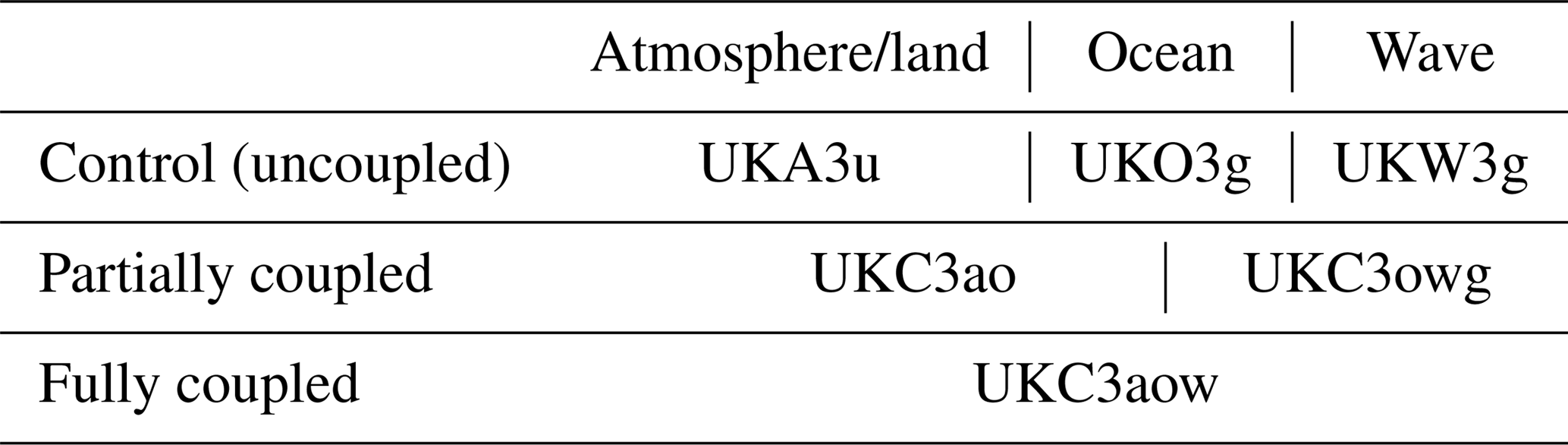
Table 10 lists the model simulations conducted for each period. Given the increased computational cost of running model experiments over longer periods, only a subset of the possible system configurations defined in Table 2 are considered here. Coupled model results from fully (UKC3aow) and partially (UKC3ao, UKC3owg) coupled mode simulations are compared with the UKA3u, UKO3g and UKW3g control simulations, as these are considered to be the most analogous to typical operational configurations currently in use.
It is considered most efficient to focus results on a relative evaluation between coupled and uncoupled simulations of the UKC3 system over the selected periods, rather than on a comparison between the UKC2 and UKC3 releases. This approach helps to isolate the impact of the new coupling capabilities within UKC3 from any other code or configuration updates between versions, and provides a more relevant summary of the relative performance of the coupled system relative to current operational approaches using more recent science configurations and code.
All simulations are initialized with the same initial conditions relevant to each model component, and the lateral boundary conditions applied are common across simulations, irrespective of the mode of running.
The following analysis compares model outputs to a variety of in situ observations taken from the Met Office operational archive. Figure 1 illustrates the typical data availability, as available for assessment of 1 day of the “Summer” 2014 experiment. Further details on the observing networks are provided by Lewis et al. (2018). Where model results are compared with observations, a “neighbourhood” of 3 by 3 grid cells nearest the observation location are considered and local mean values computed. This is considered to provide a more robust evaluation than considering only the nearest matching model grid cell for kilometre-scale model systems (e.g. Mittermaier, 2014).
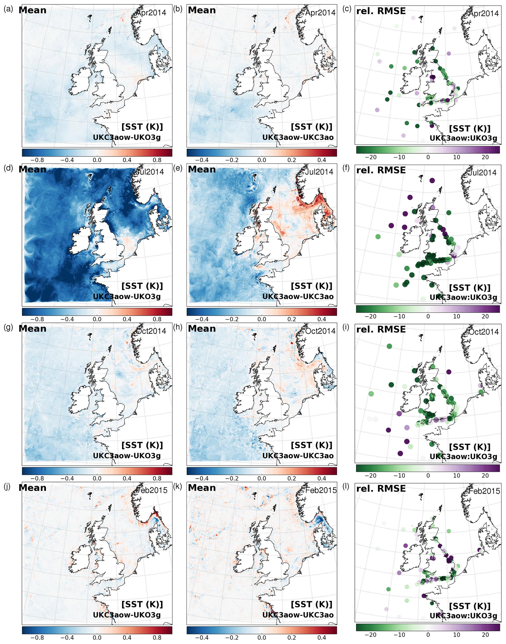
Figure 3Sensitivity of ocean model sea surface temperature (SST) to coupling. (a, d, g, j) Monthly mean difference between fully coupled and ocean only (UKC3aow–UKO3g) during April, July, October 2014 and February 2015 runs, respectively. (b, e, h, k) Monthly mean difference between fully coupled and partially coupled (UKC3aow–UKC3ao) runs during each experiment. Note the different colour scale. (c, f, i, l) Percentage difference in surface temperature RMSE statistic for UKC3aow relative to UKO3g.
4.3 Ocean component results
Figure 3 shows a summary of experiment-mean ocean model SST results across each simulation period, comparing fully coupled UKC3aow, partially coupled UKC3ao and forced-mode UKO3g configurations. The sensitivity of SST to coupling is highest during summer months as expected (e.g. Lewis et al., 2018).
The mean differences UKC3aow–UKO3g represent the impact of full atmosphere–ocean–wave coupling relative to a free-running ocean-only configuration. To a first order approximation, differences are therefore a combination of the impact of wave forcing and feedbacks on the ocean, the impact of a change in meteorological forcing resulting from increased atmospheric resolution from global (∼17 km) to regional (1.5 km) scale, and the effect of three-way coupled feedbacks between ocean and atmosphere, ocean or waves. In April, July and October runs, the impact of full coupling is a mean reduction of SST. This is typically 0.2 K in April and October, but mean changes of up to 1 K are found for the July 2014 simulations (Fig. 3d). The relative impact of wave feedbacks on both the ocean and atmosphere is illustrated in Fig. 3b, e, h and k by comparing UKC3aow with UKC3ao. This highlights a general tendency for wave coupling to cool the simulated SST, by up to 0.5 K, which is found to be mostly driven by a relatively reduced surface drag in April, July and October at least (e.g. Fig. 2b). This effect can be replicated in the partially coupled UKC3owg configuration through the wave-modified surface drag (Sect. 3.1).
The comparison between model results and in situ SST observations presented in Fig. 3 shows a general improvement in RMSE statistics, particularly at the near-coastal buoys but also more widely for UKC3aow relative to UKO3g. Time series of the average ocean model bias for SST through each simulation are shown in Fig. 4. This highlights that the UKO3g ocean-only simulation is generally biased warm for each season, and by up to 1 K during the July 2014 run. Note that all simulations are initialized from a multi-annual run of the UKO3g ocean configuration. For the July 2014 experiment, while UKO3g results maintain the initial bias of approximately 1 K too warm throughout the month-long simulation, the initial bias is eroded over the first week or so of simulations to be approximately 0.2 K too warm in both UKC3ao and UKC3aow runs, and is further reduced in the last week of the simulation. Similar features but of smaller magnitude can be seen during April and October 2014 experiments. This result is found to be a function of both the spatial and/or temporal resolution change (noting that the UKO3g forcing is obtained from operational archives with data assimilation) in the atmosphere forcing, and a result of an improved atmospheric state due to the dynamic coupling to the ocean (and wave) component. The magnitude of improvements due to coupled relative to observations is further highlighted for these months in Fig. 4b, d and f which show the time series of the absolute model bias relative to the UKO3g control.
The contribution of wave processes to the reduction in SST bias can be determined in fully coupled mode by comparing UKC3aow and UKC3ao results (dark red relative to light red in Fig. 4), and in partially coupled mode with consistent atmospheric forcing by comparing UKC3owg with ocean-only UKO3g (blue relative to grey line in Fig. 4). This shows representation of wave processes to improve the agreement of simulated SST with observations, but also that this contribution is estimated to be approximately 10 % of the differences between fully coupled and ocean-only modes. A larger relative improvement is also found in forced mode (UKC3owg–UKO3g) than found between UKC3aow and UKC3ao in April and July 2014 at least.
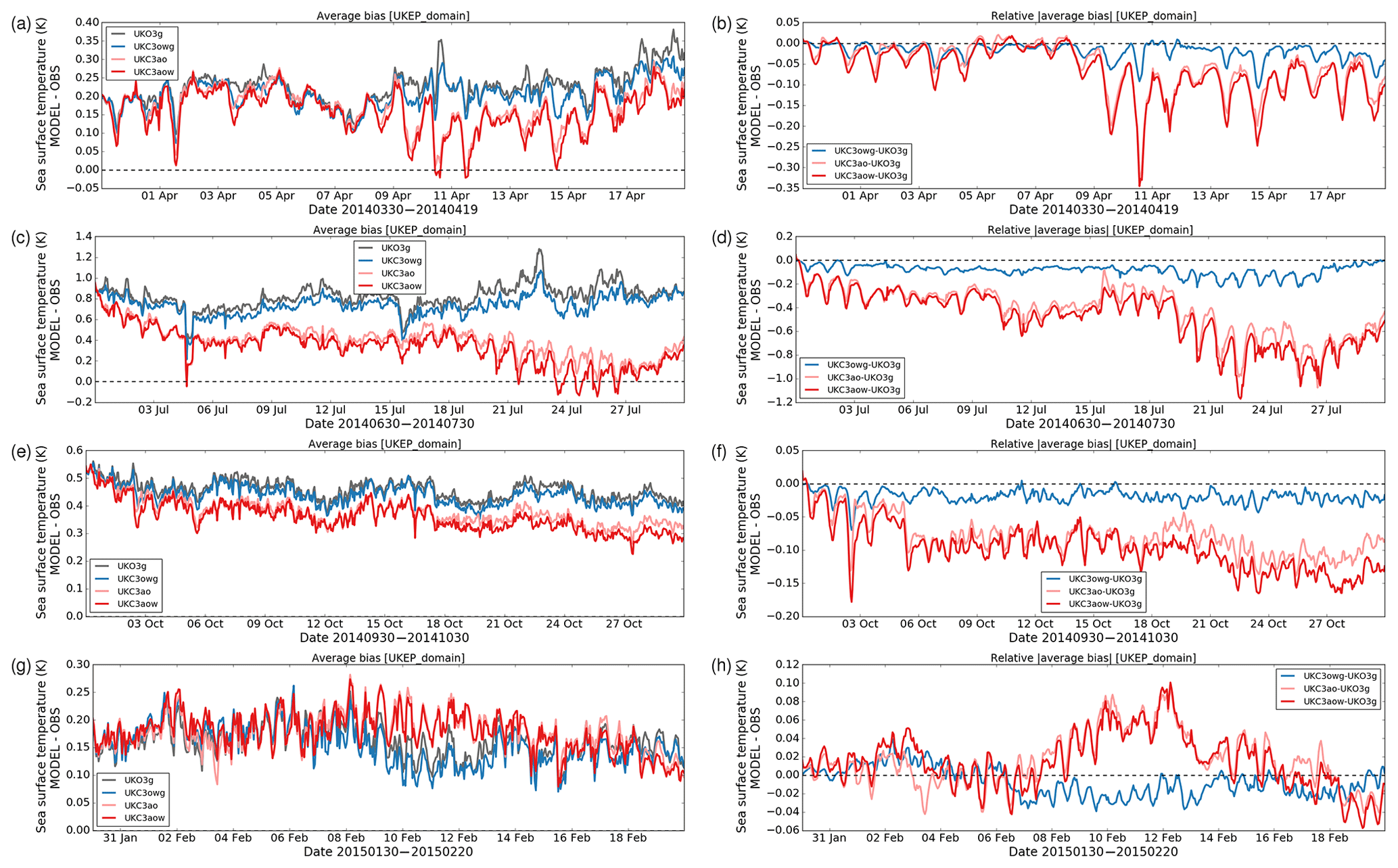
Figure 4(a, c, e, g) Time series of average model–observation (MODEL–OBS) bias of ocean model sea surface temperature across all observing sites for each simulation for July, April, October 2014 and February 2015, respectively. (b, d, f, h) Differences in absolute |MODEL–OBS| bias for each simulation period relative to UKA3u. A negative relative |average bias| indicates the coupled system to have a lower average absolute bias across all observation sites than the control. Note that plots have different scales across the different months evaluated, and observations are compared with a nearest neighbourhood mean of 3 by 3 model grid cells.
Results for a winter month (February 2015) show the impact of full coupling and wave feedbacks to be more isolated to near-coastal areas, and while improvements in RMSE for UKC3aow relative to UKO3g can be seen in Fig. 3l, the relative difference in mean bias in Fig. 4h fluctuates through the month (but typically within 0.1 K). In this case, the impact of wave feedbacks is generally very similar between UKC3aow and UKC3owg simulations relative to UKO3g.
This discussion highlights the potential of regional coupled systems to deliver improved simulation of the ocean state, and this development is being tested for implementation within the framework of the EU Copernicus Marine Environment Monitoring Service (CMEMS) for the north-west European shelf region for example.
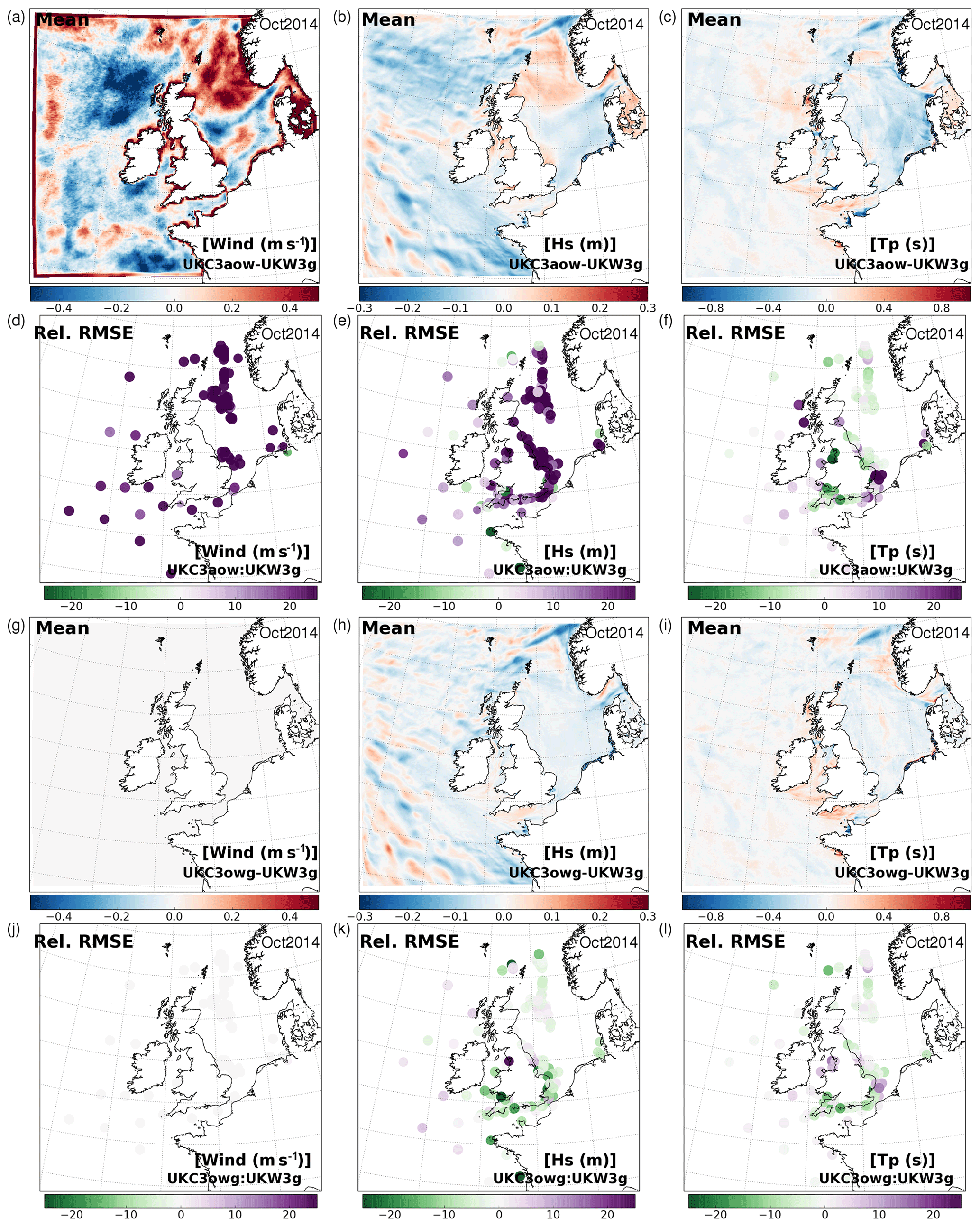
Figure 5Sensitivity of wave model wind forcing, significant wave height (Hs) and peak wave period (Tp) to coupling during October 2014 experiment. Monthly mean differences between UKC3aow and UKW3g for (a) coupled/forced atmosphere winds, (b) significant wave height Hs and (c) peak wave period Tp. (d–f) Percentage difference in RMSE statistic for UKC3aow results relative to UKW3g for (d) wind forcing, (e) Hs, (f) Tp. (g–i) Monthly mean differences between partially coupled UKC3owg and UKW3g (i.e. with same global-scale wind forcing) for (g) wind forcing, (h) Hs, (i) Tp, and (j–l) percentage difference in RMSE statistics for each variable for UKC3owg relative to UKW3g.
4.4 Wave component results
It is widely known that the quality of the wave model results is critically dependent on the quality of the wind forcing, or that applied via atmosphere–wave coupling (e.g. Cavaleri et al., 2018). The benefit of coupling on wave results was therefore characterized by Lewis et al. (2018) for case study simulations through comparing UKC2aow results with the UKW2h control using a comparably high-resolution wind forcing, and it was found to be generally difficult to improve on the performance of the wave-only simulations forced by operational archive global resolution MetUM winds in the UKW2g configuration. The same characteristics are found for UKC3 results in this study, in which the fully coupled UKC3aow runs are compared only with partially coupled UKC3owg and forced mode UKW3g simulations in which the wind forcing is provided by the global resolution operational MetUM archive. Figure 5 illustrates the differences in wind forcing during the October 2014 experiment, which is representative of results for other months. The impact of atmosphere model resolution can be seen in particular around the coasts, where the UKC3aow winds exceed those from the global MetUM forcing. This is a combination of the effect of increased drag over land impacting a broader region in the global-scale forcing than at high resolution, and from including currents and tidal feedbacks in the lower boundary condition in the coupled configuration.
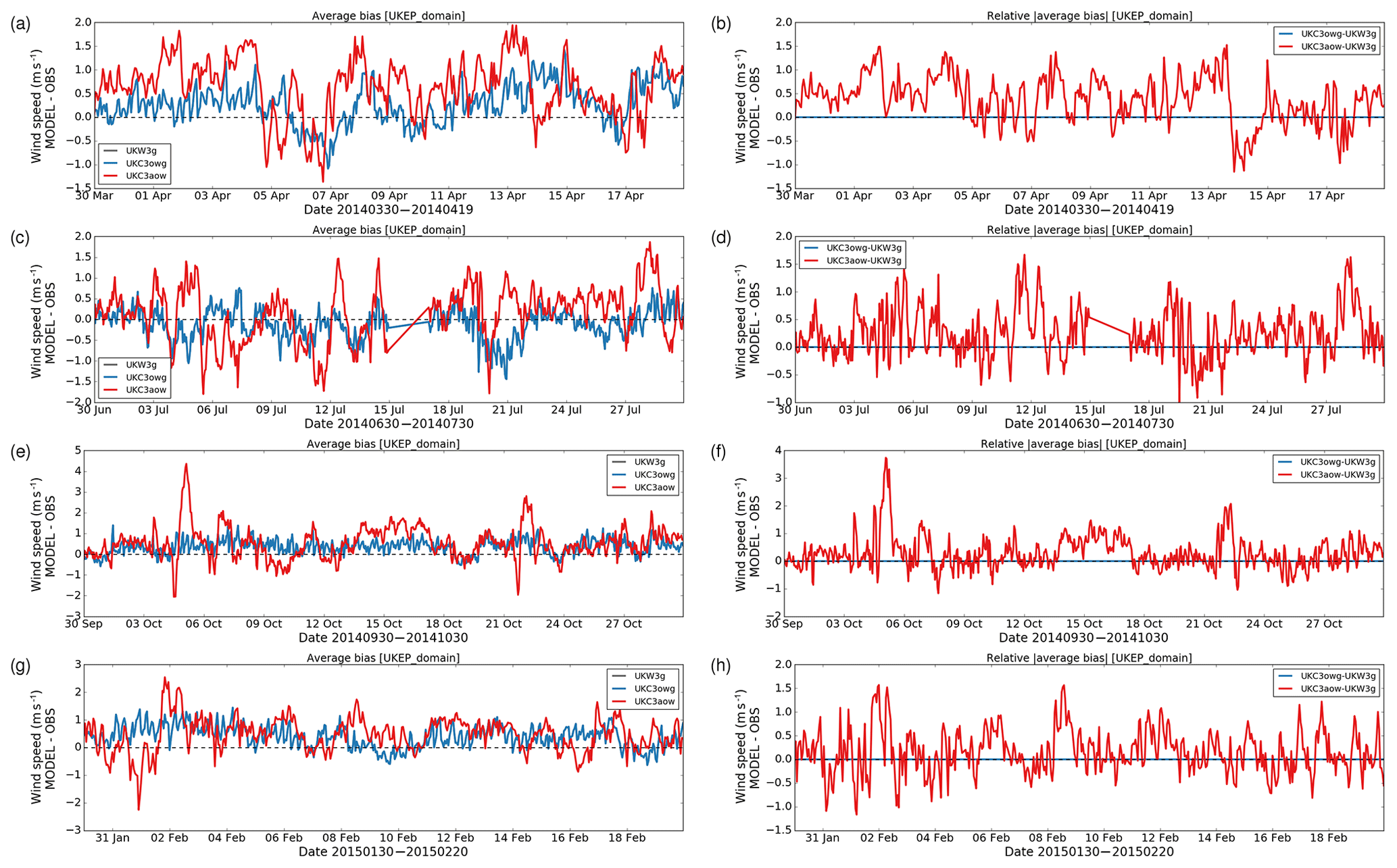
Figure 6Difference of wind forcing applied to wave model. (a, c, e, g) Time series of average model–observation (MODEL–OBS) bias across all observing sites for each simulation for July, April, October 2014 and February 2015, respectively. (b, d, f, h) Differences in absolute |MODEL–OBS| bias for each simulation period relative to the UKW3g wind forcing. Note that plots have different scales across the different months evaluated, and observations are compared with a nearest neighbourhood mean of 3 by 3 model grid cells.
Wind speeds tend to be slightly reduced in regions away from coastlines across the north-western and south-western approaches to the UK, and across the southern North Sea. These features are generally replicated during other months.
Comparison with available in situ wind observations located in the ocean (Fig. 5d), noting these are generally located away from near-coastal areas, demonstrate a consistent reduction in quality of winds at high resolution in UKC3aow relative to the global archive MetUM forcing. Figure 6 presents a more quantitative analysis through each experiment, and shows that, on average, the UKW3g (and UKC3owg) forcing is biased fast by up to 1 m s−1 during each run across the domain. The fully coupled UKC3aow winds are by contrast biased fast by up to 2 m s−1 during the four periods, but with much greater variability in the magnitude and sign of the bias through time than found for the UKW3g MetUM forcing. The fast bias is consistent with the recent analysis by Jiménez and Duidha (2018) who compared WRF model simulations with observations from the FINO (Forschungsplattformen in Nord- und Ostsee) towers located in the southern North Sea.
Figure 5b demonstrates the close link between wind speed differences between configurations and their impact on significant wave height, Hs, with increased wind speeds in UKC3aow over the northern North Sea on average tending to drive waves of increased magnitude, and reduced wave heights to the west of the UK in the fully coupled UKC3aow simulations relative to the wave-only UKW3g control. Figure 5e also highlights an expected general reduction in the level of agreement between UKC3aow wave height simulations with in situ observations relative to UKW3g. However, even given the degraded wind speed forcing, relative improvement can be seen at a number of near-coastal sites along the south-western English Channel coast.
To isolate the impact of wave–ocean feedbacks from the wind forcing, Fig. 5h and k compares UKC3owg with UKW3g results. This shows a general reduction of significant wave height in most areas, but a region of slightly enhanced wave heights along the northern half of the English Channel, associated with wave–current interactions. The impact of current–wave interactions in the near coastal zone was also discussed by Lewis et al. (2018). In contrast to Fig. 5e, wave–ocean interaction is shown to have a clear beneficial impact on the agreement between observed and simulated wave height in Fig. 5k.
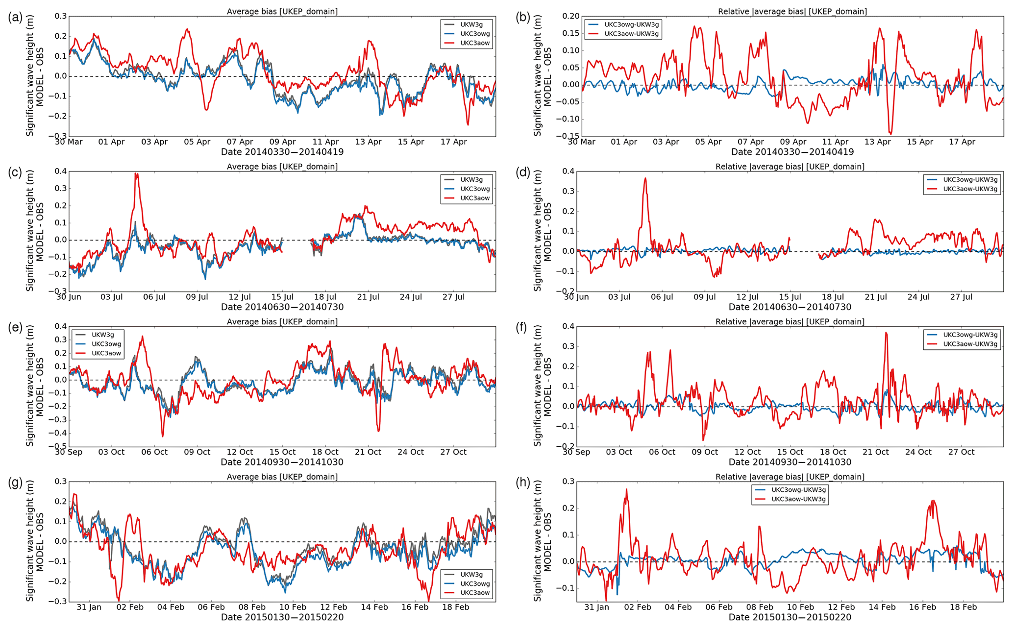
Figure 7Sensitivity of wave model significant wave height (Hs) to coupling. (a, c, e, g) Time series of average model–observation (MODEL–OBS) bias across all observing sites for each simulation for July, April, October 2014 and February 2015, respectively. (b, d, f, h) Differences in absolute |MODEL–OBS| bias for each simulation period relative to UKW3g. Note that plots have different scales across the different months evaluated, and observations are compared with a nearest neighbourhood mean of 3 by 3 model grid cells.
The time series of average model–observation bias (MODEL-OBS) in Hs shown in Fig. 7 during each experiment period reflect a tendency for the global-scale wind driven UKW3g and UKC3owg simulations to under-predict significant wave heights across all months considered by up to 0.2 m on average. The sensitivity to coupling is found to be generally consistent across the different months. The increase in wave heights through enhanced winds in the fully coupled UKC3aow system tends to improve the bias for some periods during each month. However, there are as many periods when UKC3aow results become biased high relative to observations. On average, the impact of representing ocean–wave feedback processes in UKC3owg is shown to be relatively small (within 0.05 m) in comparison with the wind-related UKC3aow differences, with no clear improvement or degradation in performance across the experiments considered.
Figure 5 also shows the impact of coupling on peak wave period during the October 2014 experiment. Results are particularly improved along the south English coast for both UKC3aow (Fig. 5f) and UKC3owg (Fig. 5l). This is consistent with the case study results of Lewis et al. (2018a), and with Palmer and Saulter (2016). They found that the inclusion of surface currents in the Met Office UK4 operational wave system improved the representation of swell in this region. This was largely due to the refraction of long-period waves towards the coast due to wave–current interaction (evident in Fig. 5c and i). The reduction in quality of peak wave period results against observations along the south-eastern English coast in Fig. 5f is not apparent for UKC3owg (Fig. 5l), suggesting that the wind speed errors continue to dominate here.
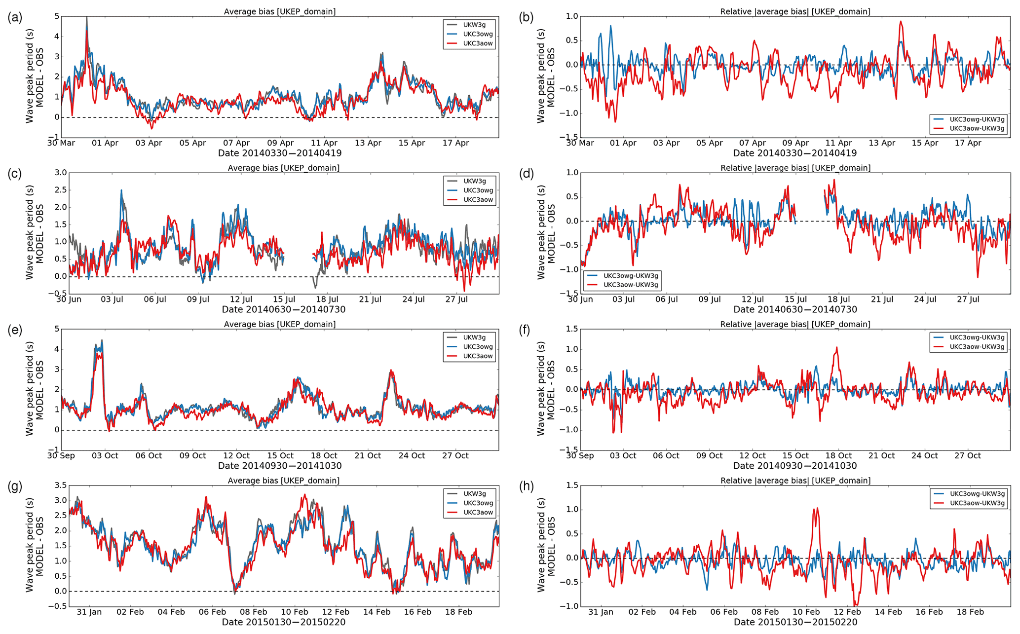
Figure 8Sensitivity of wave model peak wave period (Tp) to coupling. (a, c, e, g) Time series of average model–observation (MODEL–OBS) bias across all observing sites for each simulation for July, April, October 2014 and February 2015, respectively. (b, d, f, h) Differences in absolute |MODEL–OBS| bias for each simulation period relative to UKW3g. Note that plots have different scales across the different months evaluated, and observations are compared with a nearest neighbourhood mean of 3 by 3 model grid cells.
Figure 8 shows the time series of model bias of peak wave period through each experiment. This highlights all model results producing waves that are of a longer period than observed at near-coastal sites for much of the time. Both the fully coupled UKC3aow and partially coupled UKC3owg simulations provide reduced biases.
4.5 Atmosphere component results
Comparing the UKC3aow and UKC3ao atmosphere results with the UKA3u atmosphere-only control simulation provides a strong test of the system. Whereas the coupled system SST evolves according to the free-running NEMO ocean model component, the surface forcing in the UKA3u control simulation has a daily-updating analysis-based (OSTIA; Donlon et al., 2012) SST in closer agreement with observations on average. The key limitation in UKA3u is therefore that the system has no information on the diurnal cycle of SST.
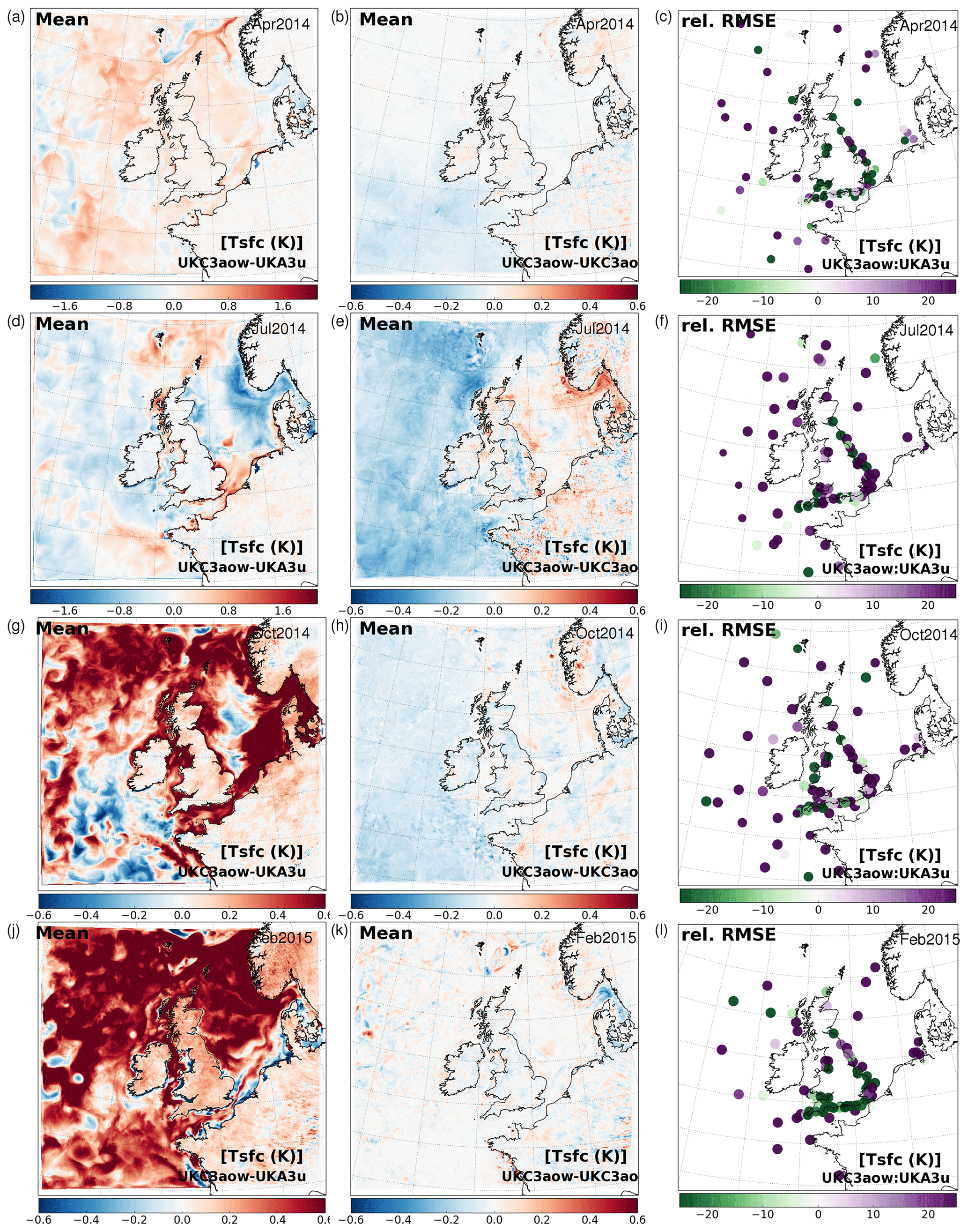
Figure 9Sensitivity of atmosphere model surface temperature to coupling. (a, d, g, j) Monthly mean difference between fully coupled and daily-updated OSTIA (UKC3aow–UKA3u) during April, July, October 2014 and February 2015 runs, respectively. (b, e, h, k) Monthly mean difference between fully coupled and partially coupled (UKC3aow–UKC3ao) runs during each experiment. (c, f, i, l) Percentage difference in surface temperature RMSE statistic for UKC3aow relative to UKA3u.
Figure 9 summarizes differences in the surface temperature across both land and sea in UKC3aow fully coupled and UKC3ao partially coupled simulations relative to UKA3u. The distribution of monthly mean differences are quite varied between each month considered, reflecting both the seasonal variability in the quality of the coupled system ocean initial condition and its subsequent evolution (see Sect. 4.3). In April, October 2014 and February 2015 experiments, the coupled model SST tends to be warmer than OSTIA, while in July 2014 SST tend to be cooler away from the permanently mixed southern North Sea region and in the Celtic Sea. The impact of wave coupling processes on the SST evolution in UKC3aow relative to UKC3ao is as shown in Fig. 4 and discussed in Sect. 4.3. The comparison of results with in situ observations in Fig. 9 shows that in general the persisted SST from OSTIA better matches observations across much of the domain, as might be anticipated. However, notable areas where the UKC3aow surface temperatures are improved relative to OSTIA can be seen along at least some coastal regions in each month considered, where it is known that the satellite-based analysis product used in UKA3u is likely to be degraded by proximity to the coastline.
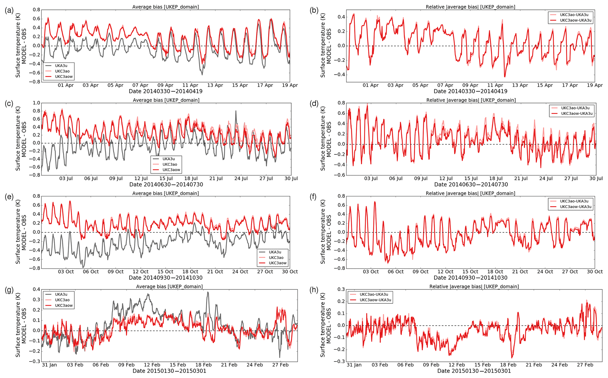
Figure 10(a, c, e, g) Time series of average model–observation (MODEL–OBS) bias of surface temperature across all observing sites for each simulation for July, April, October 2014 and February 2015, respectively. (b, d, f, h) Differences in absolute |MODEL–OBS| bias for each simulation period relative to UKA3u. A negative relative |average bias| indicates the coupled system to have a lower average absolute bias across all observation sites than the control. Note that plots have different scales across the different months evaluated, and observations are compared with a nearest neighbourhood mean of 3 by 3 model grid cells.
Noting the relatively large number of near-coastal sites contributing to the assessment, the time series of average bias during each month in Fig. 10 also show reasonably close agreement (typically within 0.5 K; slightly lower for the fully coupled UKC3aow case) of the coupled SST results with in situ observations, and extended periods of time when results show improved SST in the coupled simulations relative to UKA3u. The results for July 2014 in particular also highlight a diurnal cycle of SST bias in UKA3u, reflecting the daily persisted SST. In contrast, the representative dynamical representation of the diurnal SST cycle in the NEMO ocean model component results in a relatively smooth variation in the average bias for UKC3aow and UKC3ao.
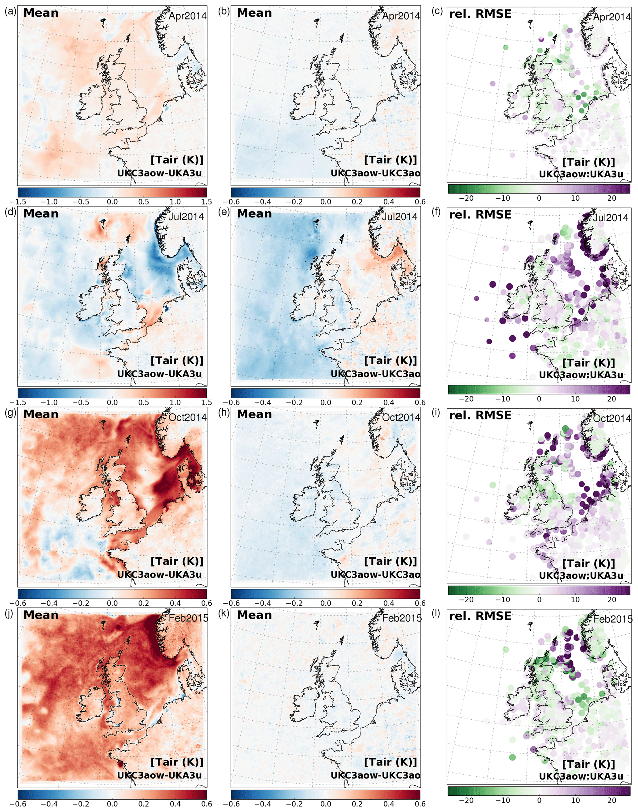
Figure 11Sensitivity of atmosphere model air temperature at 1.5 m above surface to coupling. (a, d, g, j) Monthly mean difference between fully coupled and daily-updated OSTIA (UKC3aow–UKA3u) during April, July, October 2014 and February 2015 runs, respectively. (b, e, h, k) Monthly mean difference between fully coupled and partially coupled (UKC3aow–UKC3ao) runs during each experiment. (c, f, i, l) Percentage difference in air temperature RMSE statistic for UKC3aow relative to UKA3u.
The key question to address is on the extent to which these differences in the surface temperature forcing, along with resulting differences in the surface momentum budget, change the coupled system meteorology relative to UKA3u. The spatial distribution of monthly mean differences in air temperature at 1.5 m above the surface due to coupling shown in Fig. 11 closely reflect the distribution of differences in mean surface temperature (Fig. 9). Differences over the ocean are dominated by the bias between the coupled ocean simulation and OSTIA, with the contribution due to diurnal cycle differences masked in the monthly mean measures presented. Differences over land are thought to result from a combination of advection of relatively warmer (cooler) air from over a nearby warmer (cooler) ocean between simulations, and of resulting differences to boundary layer and cloud development (e.g. Fallmann et al., 2017). Figure 11 also shows a general degradation of the agreement with in situ observations of 1.5 m air temperature over much of the domain, consistent with the SST results. However, specific regions can be seen where the fully coupled UKC3aow results have reduced RMSE in each month. The time series of average bias in air temperature across all observation sites shown in Fig. 12 is dominated by errors over land, which demonstrates a clear diurnal signal of the bias in all simulations (e.g. Bush et al., 2019). Simulated temperatures are relatively too cool during daytime and too warm at night. The impact of coupling during the periods considered in this study is, in general, to consistently shift the bias (typically warmed) at all times of the day, such that the bias is apparently “improved” relative to UKA3u during daytime but degraded at nighttime when UKA3u has a warm bias. Longer periods of improved air temperature results from UKC3aow are apparent during April, October and February experiments.

Figure 12(a, c, e, g) Time series of average model–observation (MODEL–OBS) bias of 1.5 m air temperature across all observing sites for each simulation for July, April, October 2014 and February 2015, respectively. (b, d, f, h) Differences in absolute |MODEL–OBS| bias for each simulation period relative to UKA3u. A negative relative |average bias| indicates the coupled system to have a lower average absolute bias across all observation sites than the control. Note that plots have different scales across the different months evaluated, and observations are compared with a nearest neighbourhood mean of 3 by 3 model grid cells.

Figure 13Sensitivity of atmosphere model wind speed at 10 m above surface to coupling. (a, d, g, j) Monthly mean difference between fully coupled and daily-updated OSTIA (UKC3aow–UKA3u) during April, July, October 2014 and February 2015 runs, respectively. (b, e, h, k) Monthly mean difference between fully coupled and partially coupled (UKC3aow–UKC3ao) runs during each experiment. (c, f, i, l) Percentage difference in wind speed RMSE statistic for UKC3aow relative to UKA3u.
The distribution of experiment-mean 10 m wind speed changes due to model coupling are presented in Fig. 13. The differences between UKC3aow and UKC3ao highlight that the main impact of wave coupling across all months is a reduction in the monthly mean wind speed by up to 0.5 m s−1. This is consistent with the wave-model-computed Charnock parameter tending to exceed the default assumed value of 0.011 across much of the domain (e.g. Fig. 2). This effect is most prominent during stormier periods, such as the October 2014 experiment.
Figure 13 shows a more varied spatial distribution of differences between UKC3aow and UKA3u, due to a more substantial difference in SST between the simulations, in addition to the Charnock parameter coupling. Comparing Fig. 13 with Fig. 9 suggests that to first order approximation, areas of relatively increased winds align with regions of relatively increased sea surface (and air) temperatures, and those with reduced wind speeds align with regions of reduced temperatures – i.e. the mean SST and wind speed anomalies are positively correlated. A growing literature has developed over recent years on the extent to which ocean temperature deviations drive atmospheric responses or vice versa at mesoscales in different regions of the world (e.g. Small et al., 2008; Gemmrich and Monahan, 2018). Figure 14 provides an initial assessment of the variability in monthly mean wind speed differences between simulations over the sea with differences in the near-surface temperature gradient (estimated as Tair−SST) and with differences in surface currents. This shows that where mean (land and sea) surface temperatures are increased (decreased) in UKC3aow relative to UKA3u, the impact tends to be a reduction (increase) in the near-surface temperature gradient. According to surface layer theory, under increasingly unstable conditions (change in stability < 0), the surface drag is increased and the near-surface wind speed is expected to increase (change in wind speed > 0). This mechanism is at least partly demonstrated by the variability of mean wind speed and near-surface temperature gradient differences shown in Fig. 14b. This contrasts with no clear relationship evident between wind speed and surface current differences in Fig. 14c. Corresponding results for UKC3aow and UKC3ao differences in Fig. 14 also show no strong dependencies between variables, highlighting the wind speed differences to be largely driven by the use of the wave model Charnock parameter in UKC3aow.

Figure 14Scatter plots showing relationships between differences in monthly mean results during July 2014 of (a, d) near-surface temperature difference (1.5 m air temperature − SST) with differences in SST, (b, e) 10 m wind speed with near-surface temperature difference and (c, f) 10 m wind speed with differences in surface current speed. Plots in (a)–(c) compare mean UKC3aow and UKA3u differences (i.e. fully coupled relative to atmosphere-only simulation). Plots in (d)–(f) compare mean UKC3aow and UKC3ao differences (i.e. fully coupled with wave relative to partially coupled atmosphere–ocean coupled).
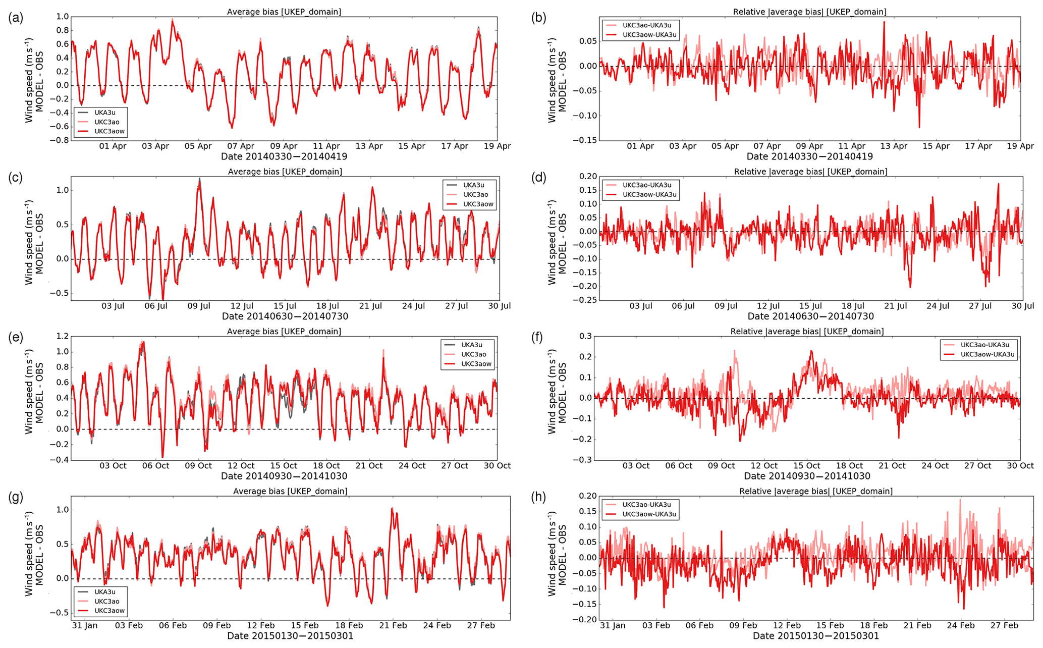
Figure 15(a, c, e, g) Time series of average model–observation (MODEL–OBS) bias of 10 m wind speed across all observing sites for each simulation for July, April, October 2014 and February 2015, respectively. (b, d, f, h) Differences in absolute |MODEL–OBS| bias for each simulation period relative to UKA3u. A negative relative |average bias| indicates the coupled system to have a lower average absolute bias across all observation sites than the control.
Table 11Summary of computer resource usage and typical runtimes and volume of data outputs generated for each day of simulation of UKC3 systems. Note further optimizations of system node usage and runtimes are possible.
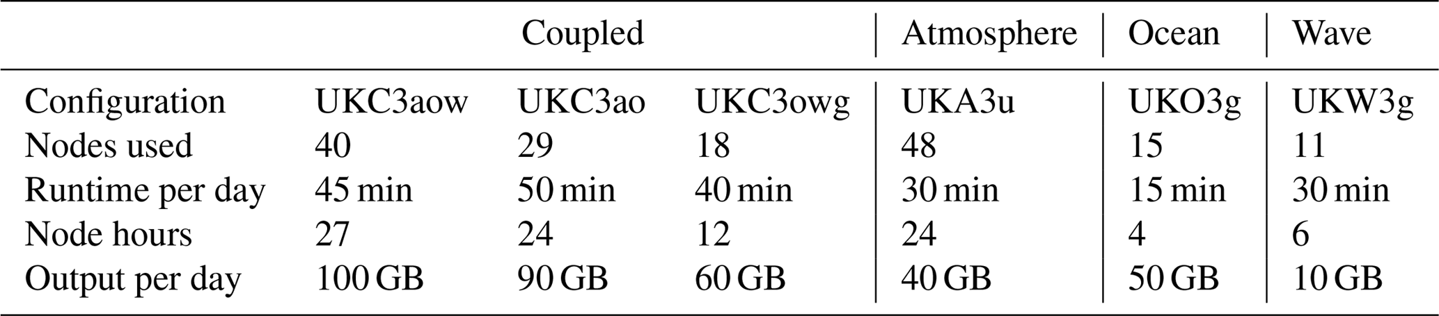
In common with air temperature results in Fig. 12, the time series of wind speed model bias for all simulations shown in Fig. 15 also demonstrate a diurnal cycle across all configurations, with winds too strong by up to 1 m s−1 on average during daytime and slightly too weak at night. As an average across all sites, the relative impact of coupling is less pronounced than found for temperature variables, with changes due to ocean–atmosphere coupling within 0.1 m s−1 for much of the periods considered. The impact of Charnock coupling is evident with improved results for UKC3aow relative to UKC3ao, and extended periods where the UKC3aow winds are improved relative to UKA3u, despite the improved SST specification in UKA3u. Results are consistently improved for UKC3aow during the February experiment for example. In contrast, from 15 October 2014, Fig. 15 shows both UKC3ao and UKC3aow simulations are degraded relative to the UKA3u control, coinciding with a period of relatively poorer surface temperature bias.
Despite the strong test set by comparing UKC3aow and UKC3ao performance to the atmosphere-only UKA3u control, these results demonstrate that representative simulations of the atmosphere can be performed in fully coupled mode at convective scales. It is clear that inclusion of the two-way feedbacks between surface waves and both ocean and atmosphere components provides some benefit over only including ocean–atmosphere feedbacks. The impact of coupling on the atmospheric boundary layer and associated features such as cloud development and near-surface visibility are the subject of ongoing research, focussing on more specific case studies periods and regions of interest (e.g. Fallmann et al., 2019).
4.6 Computational resource
Table 11 summarizes the typical computational resource usage and runtimes for a day of simulation on the Met Office Cray XC40 for each configuration used. No system optimization has been performed for UKC3, relative to the UKC2 configuration, and further opportunities for system optimization remain that will be pursued as part of the future UKC4 development, in particular relating to efficiency of the wave coupling. Previous ocean modelling research (e.g. Brown et al., 2011; Reza Hashemi et al., 2015) has commented on the large cost increase occurred due to wave coupling. Table 11 indicates that the UKO3 and UKW3 ocean-only and wave-only models used a relatively small amount of computational resource to run a day of simulation (4 and 6 node hours, respectively), and that using 12 node hours for a day of ocean–wave coupled simulation represents a big jump. However, this is not considered to be prohibitively expensive for research applications. In contrast, the computational impact of coupling in UKC3aow and UKC3ao is small, given that the regional atmosphere component is a relatively expensive part of the system.
This paper has provided an update on the evolution of a regional atmosphere–ocean–wave coupled prediction system for the UK at kilometre-scale resolution. The UKC3 system represents a further important development through the successful introduction and testing of a number of wave-to-ocean feedback processes and related data exchanges, such that for the first time UKC3aow provides a coupled system with two-way feedbacks represented between atmosphere, ocean and wave components.
The four monthly experiments presented here also represent the first runs conducted of the UKC3 (or UKC2) system of extended duration beyond the 5-day case study duration simulations described by Lewis et al. (2018), or used in the studies of Fallmann et al. (2017, 2019). That the results continue to show robust and representative predictions across atmosphere, ocean and surface wave components in coupled mode throughout these periods provides confidence in the scientific integrity of these tools, and of their suitability for application over longer timescales in future. The quality and limitations of the UKC3 system relative to uncoupled approaches has been discussed.
A number of summary results have been presented in this paper, either as monthly mean differences between coupled and uncoupled simulations or time series of the average biases between model and observations across a number of in situ observing sites through each experiment. This only provides an initial and top-level snapshot of model performance. Evidence from these experiments and Lewis et al. (2018) indicate that representing feedbacks between components adds skill to the modelling system in specific situations and at certain locations, such that any impacts can be damped in a presentation of results aggregated in time or space. In order to guide development priorities and improvement, further analysis is required to examine the specific locations and time periods for which model performance is particularly degraded or improved by coupling across any of the components of interest. This case study mode work is ongoing and will be reported through further publications.
The biggest impact of simulating in coupled mode, relative to the uncoupled configuration most analogous to current operational approaches, has been demonstrated in the ocean component SST, with a marked decrease in model bias achieved through April, July and October 2014 experiments, in part due to inclusion of wave processes in the ocean, and largely as a result of using the coupled high-resolution atmospheric forcing rather than the operational global-scale MetUM forcing.
Such general improvements were not apparent for the wave model results in contrast, given the comparison to a wave-only model forced by winds from the same operational global-scale MetUM forecasts. The improved quality and lower variability in wind forcing into UKW3g continues to drive improved quality simulation of wave height and mean period at most sites. However, for a given atmospheric forcing, the positive impact of representing wave–ocean feedbacks on results has been demonstrated. Better understanding and improving the impact of atmosphere spatial (and temporal) resolution of wind forcing or coupled information remains a priority for future development in order that wave model results within the fully coupled system might be improved relative to wave-only approaches forced by global-scale winds.
The atmosphere component results also highlight that the coupled system inherits a number of the underpinning model biases associated with convective-scale MetUM configurations, with representation of a diurnal temperature cycle through ocean–atmosphere coupling and dynamic evolution of surface roughness through wave–atmosphere coupling neither substantially degrading nor improving predictions, on average. More detailed testing of the boundary layer sensitivity to surface processes at convective scale will be of benefit for future improvement.
Having developed a fully coupled UKC3 research tool, and demonstrated its application over an extended period of time, the priorities for ongoing research and improvement can be summarized as follows.
Improving predictability
Improving skill beyond the UKC3 capability presented in this paper will require two key developments. Firstly, a number of the parameterization and parameter assumptions embedded across the MetUM atmosphere, NEMO ocean and WAVEWATCH III wave model codes, and their configuration in the regional system, will need to be re-examined and challenged. The UKC3 configuration still represents a “first look” implementation, in which a number of the underpinning assumptions and parameter choices established with uncoupled mode forcing or boundary data continue to exist. For example, consistent treatment of the atmospheric surface layer momentum budget across all codes has been an area of focus through the implementation of the wave-modified drag feedbacks within UKC3. The extent to which coupled mode running of these components is working against existing tuning is to be assessed. The influence of wind forcing on the skill of the wave model is a key example. The coupling exchange frequency is a further area deserving further study and optimization, given that the hourly coupling used in the UKC3 experiments presented in this paper is long relative to most studies discussed in Sect. 1.
Secondly, it is appropriate to begin developing the regional coupled system in an assimilative context, in order to improve the initial condition errors inherent within the current experimental design, as seen in the ocean SST results here for example. This is also a key step towards consideration of such systems for operational applications. Wada and Kunii (2017) have recently demonstrated the successful application of a regional mesoscale strongly coupled atmosphere–ocean data assimilation, implementing a local ensemble transform Kalman filter, for a tropical cyclone case study. For the UK regional coupled system development, it is more likely that a weakly coupled assimilation approach will be followed building on experience of developing this system for global coupled Numerical Weather Prediction (NWP) applications at the Met Office (e.g. Lea et al., 2015). It is not immediately clear how moving to an assimilative framework will modify any sensitivity to coupling, if at all, and research is clearly required in this area. One hypothesis is that the observational constraint will reduce the relative impact of representing feedback processes in the system. Conversely, improving the background state through improving the physics representation may in fact enhance the impact of data assimilation within the system by reducing the background errors. Even assimilation of observations in only one component may result in beneficial impacts across other model components. One particularly beneficial development that will support future research in this area is the implementation of analogous operational UK variable-resolution (UKV) atmosphere (e.g. Bush et al., 2019) and AMM15 ocean configurations (e.g. Graham et al., 2018) for operational forecasting at the Met Office using common physics settings, domain extent and grid definition to those used in UKC3. These provide the potential for operational analyses and boundary conditions for application in future regional coupled research activities.
Towards integrated environmental prediction capability
The focus of this paper has been on the physical coupling processes across atmosphere, ocean and wave components, with the driver of improving predictability through improved physical process representation. The vision for regional coupled prediction systems is that they can also provide a framework in which to represent interactions and feedbacks between physical, hydrological and biogeochemical cycles and processes at kilometre-scale. The initial focus in this context remains to demonstrate coupled prediction of the water cycle across atmosphere, land and ocean. Improvements to the convective rainfall representation and improved accuracy of quantitative precipitation forecasts in the UKC3 (RA1 physics) configuration relative to that in the UKC2 system (Bush et al., 2019) forms a key foundation of turning that potential into a reality. Further improvements to the hydrological capability in the JULES land surface model are also planned (e.g. Martínez-de la Torre et al., 2018), and their impact will be documented in the context of developing the UKC4 system.
Feedbacks between physical and biogeochemical processes in the ocean will also be introduced. A first required step is the technical implementation of the ERSEM (European Regional Seas Ecosystem Model; Butenschön et al., 2016) marine biogeochemical model as a new coupled component into the UKC4 system.
Longer-term considerations
The potential for delivering consistent natural hazard warnings across the scope of atmosphere, land, ocean and wave components was introduced in Sect. 1. Application of the UKC3 and its subsequent iterations to demonstrating this concept is still required. A key part of realizing this vision in a more operational context, particularly for hydrological and surge hazards for example, will be the requirement to develop an ensemble of regional coupled predictions. Consideration will need to be given on how to generate a regional ensemble with adequate spread in ocean and land surface states in the short term, with opportunities again to build on experience from the development of global-scale coupled NWP (e.g. Tennant and Beare, 2014). Incremental improvements to the capability and application of the UK regional coupled system will therefore continue over coming years, with the UKC3 system configuration providing an important milestone along that research journey. This effort will continue to require a multi-disciplinary approach, working in open collaboration both in the UK and with other groups around the world.
5.1 Code availability
Intellectual property
Due to intellectual property right restrictions, neither the source code nor documentation papers for the Met Office Unified Model or JULES can be provided directly. All model codes used within the UKC3 configuration are accessible to registered researchers, and links to the relevant code licences and registration pages are provided for each modelling system below. All code used can be made available to the Editor for review. Supplement to this paper does include a set of Fortran namelists that define the atmosphere, land, ocean and wave configurations in UKC3 simulations.
Obtaining the Met Office Unified Model
The Met Office Unified Model (MetUM) is available for use under licence. A number of research organizations and national meteorological services use the MetUM in collaboration with the Met Office to undertake basic atmospheric process research, produce forecasts, develop the MetUM code and build and evaluate Earth system models. For further information on how to apply for a licence see http://www.metoffice.gov.uk/research/collaboration/um-partnership (last access: 18 February 2019). The MetUM vn10.6 trunk code and associated modifications for UKC3 are available to registered researchers via a shared MetUM code repository, which can be accessed via https://code.metoffice.gov.uk/trac/um/wiki (last access: 18 February 2019). Details of the separate code branches with modifications for UKA3 and UKC3 are documented in the Supplement. A copy of the merged MetUM code used for UKC3 is provided at https://code.metoffice.gov.uk/trac/utils/browser/ukeputils/trunk/gmd-2018/uka3/um (last access: 18 February 2019) to support collaboration.
Obtaining JULES
JULES is available under licence free of charge. For further information on how to gain permission to use JULES for research purposes see http://jules.jchmr.org (last access: 18 February 2019). The JULES vn4.7 trunk code and associated modifications for UKC3 are then freely available on the JULES code repository, which can be accessed via https://code.metoffice.gov.uk/trac/jules/wiki (last access: 18 February 2019). Details of the separate code branches with modifications for UKA3 and UKC3 are documented in the Supplement. A copy of the merged JULES code used for UKC3 is provided for reference and to support collaboration at https://code.metoffice.gov.uk/trac/utils/browser/ukeputils/trunk/gmd-2018/uka3/jules (last access: 18 February 2019).
Obtaining NEMO
The model code for NEMO vn3.6 is freely available from the NEMO website (https://www.nemo-ocean.eu/, last access: 18 February 2019). After registration the Fortran code is readily available to researchers. Modifications to the NEMO vn3.6 trunk for UKC3 are also freely available as a copy of the merged code branches at https://code.metoffice.gov.uk/trac/utils/browser/ukeputils/trunk/gmd-2018/uko3/nemo (last access: 18 February 2019). A list of the NEMO compilation keys applied on building the merged NEMO code is provided in the Supplement. Also provided are details of the separate code branches with modifications for UKO3 and UKC3.
Obtaining WAVEWATCH III
WAVEWATCH III® is distributed under an open-source-style license to registered users through a password-protected distribution site. The licence and link to request model code can be found at the NOAA National Weather Service Environmental Modeling Center web pages at http://polar.ncep.noaa.gov/waves/wavewatch/ (last access: February 2019). The model is subject to continuous development, with new releases generally becoming available after implementation of a new model version at NCEP. Research model versions may also be made available to those interested in and committed to basic model development, subject to agreement.
The WAVEWATCH III code base is distributed by NOAA under an open-source-style licence via http://polar.ncep.noaa.gov/waves/wavewatch/wavewatch.shtml (last access: February 2019). Interested readers wishing to access the code are requested to register to obtain a license via http://polar.ncep.noaa.gov/waves/wavewatch/license.shtml (last access: February 2019). Model codes used in the UKC3 system are maintained under configuration management via a mirror repository hosted at the Met Office, and can be made available to researchers for collaboration on request, given prior approval to access WAVEWATCH III from NOAA. This is provided at https://code.metoffice.gov.uk/trac/utils/browser/ukeputils/trunk/gmd-2018/ukw3 (last access: 18 February 2019). The Supplement provides a list of the WAVEWATCH III compilation switches applied on building the wave model code.
Obtaining OASIS3-MCT
OASIS3-MCT is disseminated to registered users as free software from https://verc.enes.org/oasis (last access: 18 February 2019).
Obtaining Rose
Case study simulations and configuration control namelists were enabled using the Rose suite control utilities. Further information is provided at http://metomi.github.io/rose/doc/rose.html (last access: 18 February 2019), including documentation and installation instructions.
Obtaining FCM
All codes were built using the fcm_make extract and build system provided within the Flexible Configuration Management (FCM) tools. Met Office Unified Model and JULES codes and Rose suites were also configuration managed using this system. Further information is provided at http://metomi.github.io/fcm/doc/ (last access: 18 February 2019).
Data availability
The nature of the 4-D data generated in running the various UKC3 experiments at 1.5 km resolution requires a large tape storage facility. These data are of the order of tens of terabytes. However, these data can be made available after contacting the authors. Each simulation namelist and input data are also archived under configuration management, and can be made available to researchers to promote collaboration upon contacting the authors.
Ocean bathymetry was obtained from the EMODnet Portal: EMODnet Bathymetry Consortium, EMODnet Digital Bathymetry (DTM), EMODnet Bathymetry (September 2015 release).
| Symbol | Units | Description | Equation reference |
| Cp | m s−1 | Wave phase speed | 10 |
| cD | – | Surface exchange coefficient for momentum | 2 |
| f | – | Coriolis parameter | 4 |
| g | m s−2 | Acceleration due to gravity | 7, 9, 10 |
| Hs | m | Significant wave height | 5, 6, 11 |
| ke | – | Inverse depth scale for Stokes drift velocity profile | 5, 6, 7 |
| t | s | Time coordinate | 4 |
| tauoc | – | Normalized ocean-to-atmosphere stress fraction | 3 |
| t01 | s | Wave period | 5, 6 |
| U | m s−1 | Atmospheric wind speed | 1, 2 |
| u | m s−1 | Ocean current speed | 1, 2 |
| u∗ | m s−1 | Surface friction velocity | 9, 10 |
| vs | m s−1 | Stokes drift velocity | 4, 5, 6, 7 |
| v0 | m s−1 | Surface Stokes drift velocity | 5, 6, 7 |
| z | m | Vertical coordinate | 4, 5, 6, 7 |
| z0 | m | Surface roughness length | 8, 9, 10, 11 |
| α | – | Wave-dependent Charnock coefficient | 9 |
| ρair | kg m−3 | Air density | 1, 2 |
| ρref | kg m−3 | Surface air density | 1 |
| ρw | kg m−3 | Ocean surface density | 1 |
| τ | N m−2 | Surface stress vector | 1, 2 |
| τatm | N m−2 | Stress applied by atmosphere on ocean surface | 3 |
| τocn | N m−2 | Water-side stress transmitted into ocean | 3 |
| τwav | N m−2 | Momentum flux absorbed by wave field | 3 |
| τwav:ocn | N m−2 | Momentum released by waves to the ocean | 3 |
| ωp | s−1 | Wave peak angular frequency | 7 |
Table B1Summary of NEMO namelist configuration settings for enabling wave-to-ocean forcing or coupling in UKC3.
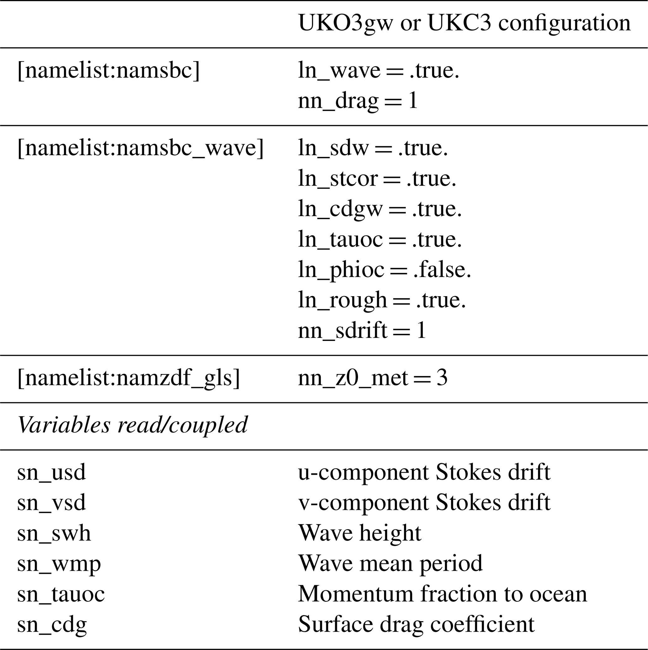
Ocean model code for wave coupling has been implemented in the NEMO trunk code, in close collaboration as part of the NEMO Wave Working Group, and supported through the Ocean-Wave-Atmosphere Interactions in Regional Seas (OWAIRS) Copernicus Marine Service Evolution project. This capability is provided in NEMO from vn4.0 including:
-
Consolidation of disparate wave science developments from contributing groups into a common code, including support for all those described in Table B1.
-
Support for required wave variables to be passed to the ocean model consistently whether in forced (file passing; core or direct flux forcing) or coupled (OASIS3-MCT library passing) mode,
-
Treatment of potentially different land/sea masks across ocean and wave models,
-
Removal of implicit assumption in NEMO that, when working in coupled mode, an atmospheric model is always coupled to NEMO,
B1 NEMO ocean model wave coupling/forcing namelist switches
To activate wave physics in NEMO in coupled mode it is necessary to specify
the same namelist variables as when running wave physics in forced mode (see
below). In addition, it would also be necessary to set the variables
ln_cpl and/or ln_wavcpl to .true. in the namelist
namsbc, while ln_mixcpl should only be .true. if there is
mixed forced runs with coupled atmosphere. Specifying
ln_wavcpl = .true. is also necessary if the coupling
is only performed to send fields from the ocean to the wave model. Remember
that when running with wave physics, it is possible to receive some wave
fields via forcing and others via coupling. The list of new NEMO namelist
variables is the following:
Namelist
namsbc:
-
Switch ln_wave: activates wave physics in both forced and coupled mode
Namelist namsbc_wave.
-
ln_sdw: modifies the surface vertical velocity due to Stokes drift; the necessary forced/coupled fields required for this option could be wave height, the two components of the surface Stokes drift, the mean wave period and the peak frequency. The specific parameterization for the calculation of the vertical Stokes drift from the surface velocity components is determined by the variable nn_sdrift (see below).
-
ln_stcor: if ln_sdw is .true., it activates the Stokes–Coriolis term; no new fields need to be read.
-
ln_cdgw: reads the neutral drag surface coefficient instead of calculating it; the field needed for this option is the surface drag coefficient. The way the momentum is calculated from the wind components is controlled by the variable nn_drag (see below). If this option is active in direct forcing of coupled mode, the variable ln_shelf_flx (namelist namsbc_flx) must be set to .true. in order to read winds instead of momentum from the input.
-
ln_tauoc: introduces a correction to the ocean stress based in the stress absorbed and/or released by the waves; the necessary field for this option is the fraction of stress that goes into the ocean.
-
ln_phioc: (not used in UKC3) adds the wave breaking mixing effect to the ocean; the necessary field for this option is the wave-to-ocean energy. The particular wave mixing TKE boundary conditions are controlled with the variable nn_wmix.
-
ln_rough: sets the surface roughness length equal to the significant wave height (making nn_z0_met = 3); the necessary field for this option is the significant wave height.
B2 NEMO ocean model wave coupling/forcing namelist parameters
A number of NEMO namelist variables need to be set depending on the values of the
namsbc_wave switches described in Sect. B1:
nn_drag (namelist namsbc; relevant when
ln_cdgw = .true.).
-
determines how to calculate wind stress from the wind components in case the wind forcing is received instead of the momentum (variable ln_shelf_flx in namelist namsbc_flx);
-
nn_drag = 0: wind stress calculated as in the ln_shelf_flx formulation, with a drag coefficient dependent on wind velocity (see Eq. 2);
-
nn_drag = 1: wind stress calculated with a coefficient that does not depend on the wind velocity, but just on the drag coefficient received via forcing or via coupling (see Eq. 3);
-
nn_drag = 2, wind stress calculated with the same formulation as for nn_drag = 1, but using a constant, default value of the drag coefficient;
-
nn_drag = 3 and running in core forcing mode, calculates the final drag coefficient using a convergence approach which needs the total precipitation and specific humidity as input parameters.
nn_sdrift (namelist namsbc_wave; relevant when ln_sdw = .true.):
-
parameterization to calculate the vertical Stokes drift from the surface components.
-
nn_sdrift = 0, use Breivik, 2015, parameterization (Breivik et al., 2015) – Eq. (6).
-
nn_sdrift = 1, use Phillips parameterization (Breivik et al., 2016) – Eq. (7).
-
nn_sdrift = 2, use Phillips parameterization with wave model peak wave number – Eq. (8).
nn_z0_met (namelist namzdf_gls; relevant when ln_rough = .true.):
-
method to calculate the surface roughness length. If the compilation key key_zdfgls or key_esopa is active and ln_rough = .true., this variable must have a value of 3.
-
nn_z0_met = 0, constant roughness is assumed – Eq. (10).
-
nn_z0_met = 1, constant Charnock formula is assumed – Eq. (11).
-
nn_z0_met = 2, Rascle et al. (2008) parameterization – Eq. (12).
-
nn_z0_met = 3, Rascle et al. (2008) with simulated wave height – Eq. (13).
B3 Forcing or coupled wave fields used by NEMO ocean model
The list of wave fields that can be received by NEMO in forced (the namelist namsbc_wave would have to be completed) or coupled mode (the namelist namsbc_cplwould have to be completed) is
-
44. Wave height (needed if ln_sdw = .true. and nn_sdrift = 0,1) – namelist variable sn_swh in forced mode and sn_rcv_hsig in coupled mode – variable name O_Hsigwa in NEMO and wavehgt in WWIII.
-
45. Normalized wave to ocean energy (needed if ln_phioc = .true.) – namelist variable sn_phioc in forced mode and sn_rcv_phioc in coupled mode – variable name O_PhiOce in NEMO and phiwvoce in WWIII.
-
46. Stokes drift in the u direction (needed if ln_sdw = .true.) – namelist variable sn_usd in forced mode and sn_rcv_sdrfx in coupled mode – variable name O_Sdrfx in NEMO and stkdrftx in WWIII.
-
47. Stokes drift in the v direction (needed if ln_sdw = .true.) – namelist variable sn_vsd in forced mode and sn_rcv_sdrfy in coupled mode – variable name O_Sdrfy in NEMO and stkdrfty in WWIII.
-
48. Mean wave period (needed if ln_sdw = .true. and nn_sdrift = 0,1) – namelist variable sn_wmp in forced mode and sn_rcv_wper in coupled mode – variable name O_WPer in NEMO and meanwper in WWIII.
-
49. Mean wave Number (needed if ln_zdfqiao = .true.) – namelist variable sn_wnum in forced mode and sn_rcv_wnum in coupled mode – variable name O_WNum in NEMO and meanwnum in WWIII.
-
50. Stress fraction into the ocean (needed if ln_tauoc = .true.) – namelist variable sn_tauoc in forced mode and sn_rcv_tauoc in coupled mode – variable name O_TauOce in NEMO and taufrac in WWIII.
-
51. Surface drag coefficient (needed if ln_cdgw = .true.) – namelist variable sn_cdg in forced mode and sn_rcv_wdrag in coupled mode – variable name O_WDrag in NEMO and dragcoef in WWIII.
-
52. Peak frequency (needed if ln_sdw = .true. and nn_sdrift = 2) – namelist variable sn_wfr in forced mode and sn_rcv_wfreq in coupled mode – variable name O_WFreq in NEMO and pkfreq in WWIII.
The value of cldes (the first parameter of the namsbc_cpl variables for wave coupling) can only be “coupled” or “none”.
B4 NEMO ocean configuration settings required for representing wave processes in forced or coupled mode
Table B1 lists the changes to NEMO namelist parameters to be set to run a direct forcing run with wave physics enabled using a baseline wave coupling parameterization with a variable Stokes drift vertical profile. Setting a coupled run is equivalent, but changing the namelist that read a particular field from forcing for a namelist that couples the same field (for example, changing sn_cdg in forced mode by sn_rcv_wdrag in coupled mode). To run in uncoupled ocean-only mode, ln_wave can be set to .false., and all wave-related NEMO namelist options are ignored.
The supplement related to this article is available online at: https://doi.org/10.5194/gmd-12-2357-2019-supplement.
HL, JMCS, AA and JF co-developed the UKC3 coupled system and carried out the experiments and analysis. Development of the component model configurations used was led by AS (wave), JG (ocean) and MB (atmosphere and land), with further significant contributions to component development and input to the coupling methodology provided by all co-authors. The research undertaken within the UK Environmental Prediction collaboration was coordinated by HL, LB, AMT and JC. HL prepared the manuscript with contributions from all co-authors.
The authors declare that they have no conflict of interest.
This research has been carried out under national capability funding as part of a directed effort on UK Environmental Prediction, in collaboration between Centre for Ecology & Hydrology (CEH), the Met Office, National Oceanography Centre (NOC) and Plymouth Marine Laboratory (PML).
Part of this work has been carried out as part of the Copernicus Marine Environment Monitoring Service (CMEMS) Ocean-Wave-Atmosphere Interactions in Regional Seas (OWAIRS) project. CMEMS is implemented by Mercator Ocean in the framework of a delegation agreement with the European Union.
We gratefully acknowledge the review comments provided for the discussion paper by an
anonymous reviewer and Bert Jagers, which led to a number of improvements and
clarifications to this paper.
Edited by: Sophie
Valcke
Reviewed by: Bert Jagers and one anonymous referee
Akan, Ç., Moghimi, S., Özkan-Haller, H. T., Osborne, J., and Kurapov, A.: On the dynamics of the Mouth of the Columbia River: Results from a three-dimensional fully coupled wave-current interaction model, J. Geophys. Res.-Oceans, 122, 5218–5236, https://doi.org/10.1002/2016JC012307, 2017
Arakawa, A. and Lamb, V. R.: Computational design of the basic dynamic processes of the UCLA general circulation model, Methods Comput. Phys., 17, 173–265, 1977.
Aranami, K., Davies, T., and Wood, N.: A mass restoration scheme for limited-area models with semi-Lagrangian advection, Q. J. Roy. Meteor. Soc., 141, 1795–1803, https://doi.org/10.1002/qj.2482, 2015.
Arnold, A.: The sensitivity of AMM15 ocean model sea surface temperature to shortwave radiation forcing, Met Office Forecasting Research Technical Report No: 627, available at: https://www.metoffice.gov.uk/binaries/content/assets/mohippo/pdf/library/weather-science-technical-reports/frtr_627_2018p.pdf (last access: 18 February 2019), 2018.
Barron, C. N., Kara, A. B., Martin, P. J., Rhodes, R. C., and Smedstad, L. F.: Formulation, implementation and examination of vertical coordinate choices in the global Navy Coastal Ocean Model (NCOM), Ocean Model., 11, 347–375, https://doi.org/10.1016/j.ocemod.2005.01.004, 2006.
Bayler, G. and Lewit, H.: The Navy Operational Global and Regional Atmospheric Prediction Systems at the Fleet Numerical Oceanography Center, Weather Forecast., 7, 273–279, https://doi.org/10.1175/1520-0434(1992)007<0273:TNOGAR>2.0.CO;2, 1992.
Best, M. J.: Representing urban areas within operational numerical weather prediction models, Bound.-Lay. Meteorol., 114, 91–109, https://doi.org/10.1007/s10546-004-4834-5, 2005.
Best, M. J., Beljaars, A. C. M., Polcher, J., and Viterbo, P.: A proposed structure for coupling tiled surfaces with the planetary boundary layer, J. Hydrometeorol., 5, 1271–1278, https://doi.org/10.1175/JHM-382.1, 2004.
Best, M. J., Pryor, M., Clark, D. B., Rooney, G. G., Essery, R. L. H., Ménard, C. B., Edwards, J. M., Hendry, M. A., Porson, A., Gedney, N., Mercado, L. M., Sitch, S., Blyth, E., Boucher, O., Cox, P. M., Grimmond, C. S. B., and Harding, R. J.: The Joint UK Land Environment Simulator (JULES), model description – Part 1: Energy and water fluxes, Geosci. Model Dev., 4, 677–699, https://doi.org/10.5194/gmd-4-677-2011, 2011.
Bidlot, J. R.: Present status of wave forecasting at ECMWF, ECMWF Workshop on Ocean Waves, Shinfield Park, Reading, UK, 25–27 June 2012, 1–15, 2012.
Bierkens, M. F. P., Bell, V. A., Burek, P., Chaney, N., Condon, L., David, C. H., de Roo, A., Döll, P., Drost, N., Famiglietti, J. S., Flörke, M., Gochis, D. J., Houser, P., Hut, R., Keune, J., Kollet, S., Maxwell, R., Reager, J. T., Samaniego, L., Sudicky, E., Sutanudjaja, E. H., van de Giesen, N., Winsemius, H., and Wood, E. F.: Hyper-resolution global hydrological modelling: what is next?, Hydrol. Process., 29, 310–320, https://doi.org/10.1002/hyp.10391, 2015.
Bohnenstengel, S. I., Evans, S., Clark, P. A., and Belcher, S.: Simulations of the London urban heat island, Q. J. Roy. Meteor. Soc., 137, 1625–1640, https://doi.org/10.1002/qj.855, 2011.
Bolaños, R., Brown, J. M., and Souza, A. J.: Wave–current interactions in a tide dominated estuary, Cont. Shelf Res., 87, 109–123, https://doi.org/10.1016/j.csr.2014.05.009, 2014.
Booij, N., Ris, R. C., and Holthuijsen, L. H.: A third-generation wave model for coastal regions: 1. Model description and validation, J. Geophys. Res.-Ocean, 104, 7649–7666, https://doi.org/10.1029/98JC02622, 1999.
Boutle, I., Price, J., Kudzotsa, I., Kokkola, H., and Romakkaniemi, S.: Aerosol–fog interaction and the transition to well-mixed radiation fog, Atmos. Chem. Phys., 18, 7827–7840, https://doi.org/10.5194/acp-18-7827-2018, 2018.
Breivik, Ø., Mogensen, K., Bidlot, J. R., Balmaseda, M. A., and Janssen, P. A. E. M.: Surface wave effects in the NEMO ocean model: Forced and coupled experiments, J. Geophys. Res.-Oceans, 120, 2973–2992, https://doi.org/10.1002/2014JC010565, 2015.
Breivik, Ø., Bidlot J.-R., and Janssen P. A.: A stokes drift approximation based on the Phillips spectrum, Ocean Model., 100, 49–56, https://doi.org/10.1016/j.ocemod.2016.01.005, 2016.
Brown, A. R., Beare, R. J., Edwards, J. M., Lock, A. P., Keogh, S. J., Milton, S. F., and Walters, D. N.: Upgrades to the boundary-layer scheme in the Met Office numerical weather prediction model, Bound.-Lay. Meteorol., 128, 117–132, https://doi.org/10.1007/s10546-008-9275-0, 2008.
Brown, A., Milton, S., Cullen, M., Golding, B., Mitchell, J., and Shelly, A.: Unified Modeling and Prediction of Weather and Climate: A 25-Year Journey, B. Am. Meteorol. Soc., 93, 1865–1877, https://doi.org/10.1175/BAMS-D-12-00018.1, 2012.
Brown, J. M., Bolaños, R., and Wolf, J.: Impact assessment of advanced coupling features in a tide–surge–wave model, POLCOMS-WAM, in a shallow water application, J. Marine Syst., 87, 13–24, https://doi.org/10.1016/j.jmarsys.2011.02.006, 2011.
Bush, M., Allen, T., Bain, C., Boutle, I., Edwards, J., Finnenkoetter, A., Franklin, C., Hanley, K., Lean, H., Lock, A., Manners, J., Mittermaier, M., Morcrette, C., North, R., Petch, J., Short, C., Vosper, S., Walters, D., Webster, S., Weeks, M., Wilkinson, J., Wood, N., and Zerroukat, M.: The first Met Office Unified Model/JULES Regional Atmosphere and Land configuration, RAL1, Geosci. Model Dev. Discuss., https://doi.org/10.5194/gmd-2019-130, in review, 2019.
Butenschön, M., Clark, J., Aldridge, J. N., Allen, J. I., Artioli, Y., Blackford, J., Bruggeman, J., Cazenave, P., Ciavatta, S., Kay, S., Lessin, G., van Leeuwen, S., van der Molen, J., de Mora, L., Polimene, L., Sailley, S., Stephens, N., and Torres, R.: ERSEM 15.06: a generic model for marine biogeochemistry and the ecosystem dynamics of the lower trophic levels, Geosci. Model Dev., 9, 1293–1339, https://doi.org/10.5194/gmd-9-1293-2016, 2016.
Byrne, D., Papritz, L., Frenger, I., Münnich, M., and Gruber, N.: Atmospheric Response to Mesoscale Sea Surface Temperature Anomalies: Assessment of Mechanisms and Coupling Strength in a High-Resolution Coupled Model over the South Atlantic, J. Atmos. Sci., 72, 1872–1890, https://doi.org/10.1175/JAS-D-14-0195.1, 2015.
Castillo, J. M. C. and Lewis, H. W.: Evaluating and optimising the cost of coupling in the UKC2 regional system, Met Office Forecasting Research Technical Report No: 621, available at: https://www.metoffice.gov.uk/binaries/content/assets/mohippo/pdf/library/frtr_621_2017p.pdf (last access: 18 February 2019), 2017.
Cavaleri, L., Abdalla, S., Benetazzo, A., Bertotti, L., Bidlot, J.-R., Breivik, Ø., Carniel, S., Jensen, R. E., Portilla-Yandun, J., Rogers, W. E., Roland, A., Sanchez-Arcilla, A., Smith, J. M., Staneva, J., Toledo, Y., van Vledder, G. Ph., and van der Westhuysen, A. J.: Wave modelling in coastal and inner seas, Prog. Oceanogr., 167, 164–233, https://doi.org/10.1016/j.pocean.2018.03.010, 2018.
Climate change initative (CCI): https://www.esa-landcover-cci.org/ (last access: 18 February 2019), 2018.
CEH: Land Cover Map, Centre for Ecology & Hydrology, available at: https://eip.ceh.ac.uk/lcm/lcmdata (last access: 18 February 2019), 2007.
Charney, J. G. and Phillips, N. A.: Numerical integration of the quasi-geostrophic equations for barotropic and simple baroclinic flows, J. Meteor., 10, 71–99, https://doi.org/10.1175/1520-0469(1953)0102.0.CO;2, 1953.
Clark, D. B., Mercado, L. M., Sitch, S., Jones, C. D., Gedney, N., Best, M. J., Pryor, M., Rooney, G. G., Essery, R. L. H., Blyth, E., Boucher, O., Harding, R. J., Huntingford, C., and Cox, P. M.: The Joint UK Land Environment Simulator (JULES), model description – Part 2: Carbon fluxes and vegetation dynamics, Geosci. Model Dev., 4, 701–722, https://doi.org/10.5194/gmd-4-701-2011, 2011.
Clark, P., Roberts, N., Lean, H., Ballard, S. P., and Charlton-Perez, C.: Convection-permitting models: a step-change in rainfall forecasting, Meteorol. Appl., 23, 165–181, https://doi.org/10.1002/met.1538, 2016.
Cosby, B. J., Hornberger, G. M., Clapp, R. B., and Ginn, T. R.: A Statistical Exploration of the Relationships of Soil Moisture Characteristics to the Physical Properties of Soils, Water Resour. Res., 20, 682–690, https://doi.org/10.1029/WR020i006p00682, 1984.
Craig, P. D. and Banner, M. L.: Modeling wave-enhanced turbulence in the ocean surface layer, J. Phys. Oceanogr., 24, 2546–2559, https://doi.org/10.1029/2007JC004246, 1994.
Dee, D. P., Uppala, S. M., Simmons, A. J., Berrisford, P., Poli, P., Kobayashi, S., Andrae, U., Balmaseda, M. A., Balsamo, G., Bauer, P., Bechtold, P., Beljaars, A. C. M., van de Berg, I., Biblot, J., Bormann, N., Delsol, C., Dragani, R., Fuentes, M., Greer, A. J., Haimberger, L., Healy, S. B., Hersbach, H., Holm, E. V., Isaksen, L., Kallberg, P., Kohler, M., Matricardi, M., McNally, A. P., Mong-Sanz, B. M., Morcette, J.-J., Park, B.-K., Peubey, C., de Rosnay, P., Tavolato, C., Thepaut, J. N., and Vitart, F.: The ERA-Interim reanalysis: Configuration and performance of the data assimilation system, Q. J. Roy. Meteorol. Soc., 137, 553–597, https://doi.org/10.1002/qj.828, 2011.
Donelan, M. A.: On the decrease of the oceanic drag coefficient in high winds, J. Geophys. Res.-Oceans, 123, 1485–1501, https://doi.org/10.1002/2017JC013394, 2018.
Donlon, C. J., Martin, M., Stark, J. D., Roberts-Jones, J., Fiedler, E., and Wimmer, W.: The Operational Sea Surface Temperature and Sea Ice Analysis (OSTIA), Remote Sens. Environ., 116, 140–158, https://doi.org/10.1016/j.rse.2010.10.017, 2012.
Durnford, D., Fortin, V., Smith, G. C., Archambault, B., Deacu, D., Dupont, F., Dyck, S., Martinez, Y., Klyszejko, E., MacKay, M., Liu, L., Pellerin, P., Pietroniro, A., Roy, F., Vu, V., Winter, B., Yu, W., Spence, C., Bruxer, J., and Dickhout, J.: Toward an Operational Water Cycle Prediction System for the Great Lakes and St. Lawrence River, B. Am. Meteorol. Soc., 99, 521–546, https://doi.org/10.1175/BAMS-D-16-0155.1, 2018.
Dzwonkowski, B., Greer, A. T., Briseño-Avena, C., Krause, J. W., Soto, I. M., Hernandez, F. J., Deary, A. L., Wiggert, J. D., Joung, D., Fitzpatrick, P. J., O'Brien, S. J., Dykstra, S. L., Lau, Y., Cambazoglu, M. K., Lockridge, G., Howden, S. D., Shiller, A. M., and Graham, W. M.: Estuarine influence on biogeochemical properties of the Alabama shelf during the fall season, Cont. Shelf Res., 140, 96–109, https://doi.org/10.1016/j.csr.2017.05.001, 2017.
Emerton, R. E., Stephens, E. M., Pappenberger, F., Pagano, T. C., Weerts, A. H., Wood, A. W., Salamon, P., Brown, J. D., Hjerdt, N., Donnelly, C., Baugh, C. A., and Cloke, H. L.: Continental and global scale flood forecasting systems, WIRES Water, 3, 391–418, https://doi.org/10.1002/wat2.1137, 2016.
Fallmann, J., Lewis, H., Castillo, J., Arnold, A., and Ramsdale, S.: Impact of sea surface temperature on stratiform cloud formation over the North Sea, Geophys. Res. Lett., 44, 4296–4303, https://doi.org/10.1002/2017GL073105, 2017.
Fallmann, J., Lewis, H., Castillo, J., and Lock, A.: Impact of high-resolution ocean-atmosphere coupling on fog formation over the North Sea, Q. J. Roy. Meteor. Soc., https://doi.org/10.1002/qj.3488, online first, 2019.
Flores, R. P., Rijnsburger, S., Horner-Devine, A. R., Souza, A. J., and Pietrzak, J. D.: The impact of storms and stratification on sediment transport in the Rhine region of freshwater influence, J. Geophys. Res.-Oceans, 122, 4456–4477, https://doi.org/10.1002/2016JC012362, 2017.
Forzieri, G., Feyen, L., Russo, S., Vousdoukas, M., Alfieri, L., Stephen, O., Migliavacca, M., Bianchi, A., Rojas, R., and Cid, A.: Multi-hazard assessment in Europe under climate change, Clim. Change, 137, 105–119, https://doi.org/10.1007/s10584-016-1661-x, 2016.
Frenger, I., Gruber, N., Knutti, R., and Münnich, M.: Imprint of Southern Ocean eddies on winds, clouds and rainfall, Nat. Geosci., 6, 608–612, https://doi.org/10.1038/ngeo1863, 2013.
Gemmrich, J. and Monahan, A.: Covariability of Near-Surface Wind Speed Statistics and Mesoscale Sea Surface Temperature Fluctuations, J. Phys. Oceanog., 48, 465–478, https://doi.org/10.1175/JPO-D-17-0177.1, 2018.
Graham, J. A., O'Dea, E., Holt, J., Polton, J., Hewitt, H. T., Furner, R., Guihou, K., Brereton, A., Arnold, A., Wakelin, S., Castillo Sanchez, J. M., and Mayorga Adame, C. G.: AMM15: a new high-resolution NEMO configuration for operational simulation of the European north-west shelf, Geosci. Model Dev., 11, 681–696, https://doi.org/10.5194/gmd-11-681-2018, 2018.
Gräwe, U., Holtermann, P., Klingbeil, K., and Burchard, H.: Advantages of vertically adaptive coordinates in numerical models of stratified shelf seas, Ocean Model., 92, 56–68, https://doi.org/10.1016/j.ocemod.2015.05.008, 2015.
Gronholz, A., Gräwe, U., Paul, A., and Schulz, M.: Investigating the effects of a summer storm on the North Sea stratification using a regional coupled ocean-atmosphere model, Ocean Dynam., 67, 211–235, https://doi.org/10.1007/s10236-016-1023-2, 2017.
Hackerott, J. A., Pezzi, L. P., Bakhoday Paskyabi, M., Oliveira, A. P., Reuder, J., de Souza, R. B., and de Camargo, R.: The role of roughness and stability on the momentum flux in the Marine Atmospheric Surface Layer: a study on the Southwestern Atlantic Ocean, J. Geophys. Res., 123, 3914–3932, https://doi.org/10.1002/2017JD027994, 2018.
Hasselmann, S., Hasselmann, K., Allender, J. H., and Barnett, P.: Computations and parameterisations of the nonlinear energy transfer in a gravity wave spectrum – Part 2: Parameterisations of the nonlinear energy transfer for application in wave models, J. Phys. Oceanogr., 15, 1378–1391, https://doi.org/10.1175/1520-0485(1985)0152.0.CO;2, 1985.
Hewitt, H. T., Bell, M. J., Chassignet, E. P., Czaja, A., Ferreira, D., Griffies, S. M., Hyder, P., McClean, J. L., New, A. L., and Roberts, M. J.: Will high-resolution global ocean models benefit coupled predictions on short-range to climate timescales?, Ocean Model., 120, 120–136, https://doi.org/10.1016/j.ocemod.2017.11.002, 2017.
Hirons, L. C., Klingaman, N. P., and Woolnough, S. J.: The impact of air-sea interactions on the representation of tropical precipitation extremes, J. Adv. Model. Earth Syst., 10, 550–559, https://doi.org/10.1002/2017MS001252, 2018.
Holt, J. T. and James, I. D.: An s coordinate density evolving model of the northwest European continental shelf: 1. Model description and density structure, J. Geophys. Res., 106, 14015–14034, https://doi.org/10.1029/2000JC000304, 2001.
Holt, J., Hyder, P., Ashworth, M., Harle, J., Hewitt, H. T., Liu, H., New, A. L., Pickles, S., Porter, A., Popova, E., Allen, J. I., Siddorn, J., and Wood, R.: Prospects for improving the representation of coastal and shelf seas in global ocean models, Geosci. Model Dev., 10, 499–523, https://doi.org/10.5194/gmd-10-499-2017, 2017.
Jiménez, P. A. and Dudhia, J.: On the Need to Modify the Sea Surface Roughness Formulation over Shallow Waters, J. Appl. Meteor. Climatol., 57, 1101–1110, https://doi.org/10.1175/JAMC-D-17-0137.1, 2018.
Jones, P.: ESMF_RegridWeightGen, available at: https://www.earthsystemcog.org/projects/regridweightgen/ (last access: 18 February 2019), 2015.
Jung, T., Miller, M. J., Palmer, T. N., Towers, P., Wedi, N., Achuthavarier, D., Adams, J. M., Altshuler, E. L., Cash, B. A., Kinter, J. L., Marx, L., Stan, C., and Hodges, K. I.: High-Resolution Global Climate Simulations with the ECMWF Model in Project Athena: Experimental Design, Model Climate, and Seasonal Forecast Skill, J. Climate, 25, 3155–3172, https://doi.org/10.1175/JCLI-D-11-00265.1, 2012.
Kay, A. L., Rudd, A. C., Davies, H. N., Kendon, E. J., and Jones, R. G.: Use of very high resolution climate model data for hydrological modelling: Baseline performance and future flood changes, Clim. Change, 133, 193–208, https://doi.org/10.1007/s10584-015-1455-6, 2015.
Kendon, E. J., Ban, N., Roberts, N. M., Fowler, H. F., Roberts, M. J., Chan, S. C., Evans, J. P., Fosser, G., and Wilkinson, J. M.: Do Convection-Permitting Regional Climate Models Improve Projections of Future Precipitation Change?, B. Am. Meteorol. Soc., 98, 79–93, https://doi.org/10.1175/BAMS-D-15-0004.1, 2017.
Komen, G., Cavaleri, L., Donelan, M., Hasselmann, K., Hasselmann, H., and Janssen, P. A. E. M.: Dynamics and Modelling of Ocean Waves, Cambridge University Press, 532 pp., 1994.
Kunii, M., Ito, K., and Wada, A.: Preliminary Test of a Data Assimilation System with a Regional High-Resolution Atmosphere–Ocean Coupled Model Based on an Ensemble Kalman Filter, Mon. Weather Rev., 145, 565–581, https://doi.org/10.1175/MWR-D-16-0068.1, 2017.
Larson, J., Jacob, R., and Ong, E.: The Model Coupling Toolkit: A New Fortran90 Toolkit for Building Multiphysics Parallel Coupled Models, Int. J. High Perform. C., 19, 277–292, https://doi.org/10.1177/1094342005056115, 2005.
Law Chune, S. and Aouf, L.: Wave effects in global ocean modeling: parametrizations vs. forcing from a wave model, Ocean Dynam., https://doi.org/10.1007/s10236-018-1220-2, 2018.
Lea, D. J., Mirouze, I., Martin, M. J., King, R. R., Hines, A., Walters, D., and Thurlow, M.: Assessing a New Coupled Data Assimilation System Based on the Met Office Coupled Atmosphere–Land–Ocean–Sea Ice Model, Mon. Weather Rev., 143, 4678–4694, https://doi.org/10.1175/MWR-D-15-0174.1, 2015.
Lewis, H., Mittermaier, M., Mylne, K., Norman, K., Scaife, A., Neal, R., Pierce, C., Harrison, D., Jewell, S., Kendon, M., Saunders, R., Brunet, G., Golding, B., Kitchen, M., Davies, P., and Pilling, C.: From months to minutes – exploring the value of high-resolution rainfall observation and prediction during the UK winter storms of 2013/2014, Meteorol. Appl., 22, 90–104, https://doi.org/10.1002/met.1493, 2015.
Lewis, H. W., Castillo Sanchez, J. M., Graham, J., Saulter, A., Bornemann, J., Arnold, A., Fallmann, J., Harris, C., Pearson, D., Ramsdale, S., Martínez-de la Torre, A., Bricheno, L., Blyth, E., Bell, V. A., Davies, H., Marthews, T. R., O'Neill, C., Rumbold, H., O'Dea, E., Brereton, A., Guihou, K., Hines, A., Butenschon, M., Dadson, S. J., Palmer, T., Holt, J., Reynard, N., Best, M., Edwards, J., and Siddorn, J.: The UKC2 regional coupled environmental prediction system, Geosci. Model Dev., 11, 1–42, https://doi.org/10.5194/gmd-11-1-2018, 2018.
Li, J.-G.: Upstream non-oscillatory advection schemes, Mon. Weather Rev., 136, 4709–4729, https://doi.org/10.1175/2008MWR2451.1, 2008.
Lock, A. P., Brown, A. R., Bush, M. R., Martin, G. M., and Smith, R. N. B.: A new boundary layer mixing scheme. Part I: Scheme description and SCM tests, Mon. Weather Rev., 128, 3187–3199, https://doi.org/10.1175/1520-0493(2000)128<3187:ANBLMS>2.0.CO;2, 2000.
Luiz do Vale Silva, T., Veleda, D., Araujo, M., and Tyaquiçã, P.: Ocean–Atmosphere Feedback during Extreme Rainfall Events in Eastern Northeast Brazil, J. Appl. Meteor. Climatol., 57, 1211–1229, https://doi.org/10.1175/JAMC-D-17-0232.1, 2018.
MacLachlan, C., Arribas, A., Peterson, D., Maidens, A., Fereday, D., Scaife, A. A., Gordon, M., Vellinga, M., Williams, A., Comer, R. E., Camp, J., Xavier, P., and Madec, G.: Global Seasonal forecast system version 5 (GloSea5): a high resolution seasonal forecast system, Q. J. Roy. Meteor. Soc., 141, 1072–1084, https://doi.org/10.1002/qj.2396, 2015.
Madec, G. and the NEMO team: NEMO reference manual 3_6_STABLE:NEMO ocean engine, Note du Pôle de modélisation, Institut Pierre-Simon Laplace (IPSL), France, No. 27, ISSN 1288-1619, 2016.
Marsooli, R. and Lin, N.: Numerical modeling of historical storm tides and waves and their interactions along the U.S. east and Gulf Coasts, J. Geophys. Res.-Oceans, 123, 3844–3874, https://doi.org/10.1029/ 2017JC013434, 2018.
Martínez-de la Torre, A., Blyth, E. M., and Weedon, G. P.: Using observed river flow data to improve the hydrological functioning of the JULES land surface model (vn4.3) used for regional coupled modelling in Great Britain (UKC2), Geosci. Model Dev., 12, 765–784, https://doi.org/10.5194/gmd-12-765-2019, 2019.
Miller, A. J., Collins, M., Gualdi, S., Jensen, T. G., Misra, V., Pezzi, L. P., Pierce, D. W., Putrasahan, D., Seo, H., and Tseng, Y. H.: Coupled ocean-atmosphere modeling and predictions, J. Mar. Res., 75, 361–402, https://doi.org/10.1357/002224017821836770, 2017.
Mittermaier, M. P.: A Strategy for Verifying Near-Convection-Resolving Model Forecasts at Observing Sites, Weather Forecast., 29, 185–204, https://doi.org/10.1175/WAF-D-12-00075.1, 2014.
Mogensen, K. S., Magnusson, L., and Bidlot, J.-R.: Tropical cyclone sensitivity to ocean coupling in the ECMWF coupled model, J. Geophys. Res.-Oceans, 122, 4392–4412, https://doi.org/10.1002/2017JC012753, 2017.
Oerder, V., Colas, F., Echevin, V., Masson, S., and Lemarié, F.: Impacts of the mesoscale ocean-atmosphere coupling on the Peru-Chile ocean dynamics: The current-induced wind stress modulation, J. Geophys. Res.-Oceans, 123, 812–833, https://doi.org/10.1002/2017JC013294, 2018.
Palmer, T. N.: Towards the probabilistic Earth-system simulator: a vision for the future of climate and weather prediction, Q. J. Roy. Meteor. Soc., 138, 841–861, https://doi.org/10.1002/qj.1923, 2012.
Palmer, T. and Saulter, A.: Evaluating the effects of ocean current fields on a UK regional wave model, Met Office Forecasting Research, Technical Report No: 612, available at: https://www.metoffice.gov.uk/binaries/content/assets/mohippo/pdf/j/i/frtr_612_2016p.pdf (last access: 18 February 2019), 2016.
Pullen, J., Allard, R., Seo, H., Miller, A. J., Chen, S., Pezzi, L. P., Smith, T., Chu, P., Alves, J., and Caldeira, R.: Coupled ocean-atmosphere forecasting at short and medium time scales, J. Mar. Res., 75, 877–921, https://doi.org/10.1357/002224017823523991, 2017a.
Pullen, J., Caldeira, R., Doyle, J. D., May, P., and Tomé, R.: Modeling the air-sea feedback system of Madeira Island, J. Adv. Model. Earth Syst., 9, 1641–1664, https://doi.org/10.1002/2016MS000861, 2017b.
Rainaud, R., Brossier, C. L., Ducrocq, V., and Giordani, H.: High-resolution air–sea coupling impact on two heavy precipitation events in the Western Mediterranean, Q. J. Roy. Meteor. Soc., 143, 2448–2462, https://doi.org/10.1002/qj.3098, 2017.
Rascle, N., Ardhuin, F., Queffeulou, P., and Croizé-Fillon, D.: A global wave parameter database for geophysical applications, Part 1: Wave-current–turbulence interaction parameters for the open ocean based on traditional parameterizations, Ocean Model., 25, 154–171, https://doi.org/10.1016/j.ocemod.2008.07.006, 2008.
Reza Hashemi, M., Neill, S. P., and Davies, A. G.: A coupled tide-wave model for the NW European shelf seas, Geophys. Astro. Fluid, 109, 234–253, https://doi.org/10.1080/03091929.2014.944909, 2015.
Ricchi, A., Miglietta, M. M., Barbariol, F., Benetazzo, A., Bergamasco, A., Bonaldo, D., Cassardo, C., Falcieri, F. M., Modugno, G., Russo, A., Sclavo, M., and Carniel, S.: Sensitivity of a Mediterranean Tropical-Like Cyclone to Different Model Configurations and Coupling Strategies, Atmosphere, 8, 92, https://doi.org/10.3390/atmos8050092, 2017.
Rockel, B., Will, A., and Hense, A.: The regional climate model COSMO-CLM (CCLM), Meteorol. Z., 17, 347–348, https://doi.org/10.1127/0941-2948/2008/0309, 2008.
Seo, H.: Distinct influence of air-sea interactions mediated by mesoscale sea surface temperature and surface current in the Arabian Sea, J. Climate, 30, 8061–8079, https://doi.org/10.1175/JCLI-D-16-0834.1, 2017.
Seo, H., Miller, A. J., and Roads, J. O.: The Scripps Coupled Ocean-Atmosphere Regional (SCOAR) model, with applications in the eastern Pacific sector, J. Climate, 20, 381–402, https://doi.org/10.1175/JCLI4016, 2007.
Shapiro, M., Shukla, J., Brunet, G., Nobre, C., Beland, M., Dole, R., Tremberth, K., Anthes, R., Asrar, G., Barrie, L., Bougeault, P., Brasseur, G., Burridge, D., Busalacchi, A., Caughey, J., Chen, D., Church, B., Enomoto, T., Hoskins, B., Hov, O., Laing, A., Le Treut, H., Marotzke, J., McBean, G., Meehl, G., Miller, M., Mills, B., Mitchell, J., Moncrieff, M., Nakazawa, T., Olafsson, H., Palmer, T., Parson, D., Rogers, D., Simmons, A., Troccoli, A., Toth, Z., Uccellini, L., Velden, C., and Wallace, J. M.: An Earth-System prediction initiative for the 21st Century, B. Am. Meteorol. Soc., 91, 1377–1388, https://doi.org/10.1175/2010BAMS2944.1, 2010.
Shchepetkin, A. F. and McWilliams, J. C.: The regional oceanic modeling system (ROMS): A split-explicit, free-surface, topography-following-coordinate oceanic model, Ocean Model., 9, 347–404, https://doi.org/10.1016/j.ocemod.2004.08.002, 2005.
Shimura, T., Mori, N., Takemi, T., and Mizuta, R.: Long-term impacts of ocean wave-dependent roughness on global climate systems, J. Geophys. Res.-Oceans, 122, 1995–2011, https://doi.org/10.1002/2016JC012621, 2017.
Siddorn, J. R. and Furner, R.: An analytical stretching function that combines the best attributes of geopotential and terrain-following vertical coordinates, Ocean Model., 66, 1–3, https://doi.org/10.1016/j.ocemod.2013.02.001, 2013.
Siddorn, J. R., Good, S. A., Harris, C. M., Lewis, H. W., Maksymczuk, J., Martin, M. J., and Saulter, A.: Research priorities in support of ocean monitoring and forecasting at the Met Office, Ocean Sci., 12, 217–231, https://doi.org/10.5194/os-12-217-2016, 2016.
Simpson, J. H.: Physical processes in the ROFI regime, J. Marine Syst., 12, 3–15, https://doi.org/10.1016/S0924-7963(96)00085-1, 1997.
Skamarock, W. C. and Klemp, J. B. A time-split nonhydrostatic atmospheric model for weather research and forecasting applications, J. Comput. Phys., 227, 3465–3485, https://doi.org/10.1016/j.jcp.2007.01.037, 2008.
Small, R. J., de Szoeke, S. P., Xie, S. P., O'Neill, L., Seo, H., Song, Q., Cornillon, P., Spall, M., and Minobe, S.: Air–sea interaction over ocean fronts and eddies, Dynam. Atmos. Oceans, 45, 274–319, https://doi.org/10.1016/j.dynatmoce.2008.01.001, 2008.
Smith, S. D. and Banke, E. G.: Variation of the sea surface drag coefficient with wind speed, Q. J. Roy. Meteor. Soc., 101, 665–673, https://doi.org/10.1002/qj.49710142920, 1975.
Staneva, J., Alari, V., Breivik, Ø., Bidlot, J-.R., and Mogensen, K.: Effects of wave-induced forcing on a circulation model of the North Sea, Ocean Dynam., 67, 81–101, https://doi.org/10.1007/s10236-016-1009-0, 2017.
Staneva, J., Wahle, K., Koch, W., Behrens, A., Fenoglio-Marc, L., and Stanev, E. V.: Coastal flooding: impact of waves on storm surge during extremes – a case study for the German Bight, Nat. Hazards Earth Syst. Sci., 16, 2373–2389, https://doi.org/10.5194/nhess-16-2373-2016, 2016a.
Staneva, J., Wahle, K., Günther, H., and Stanev, E.: Coupling of wave and circulation models in coastal–ocean predicting systems: a case study for the German Bight, Ocean Sci., 12, 797–806, https://doi.org/10.5194/os-12-797-2016, 2016b.
Tennant, W. and Beare, S.: New schemes to perturb sea-surface temperature and soil moisture content in MOGREPS, Q. J. Roy. Meteor. Soc., 140, 1150–1160, https://doi.org/10.1002/qj.2202, 2014.
WAVEWATCH III® Development Group (WW3DG): User manual and system documentation of WAVEWATCH III® version 5.16, Tech. Note 329, NOAA/NWS/NCEP/MMAB, College Park, MD, USA, 326 pp. + Appendices, 2016.
Umlauf, L. and Burchard, H.: A generic length-scale equation for geophysical turbulence models, J. Marine Res., 61, 235–265, https://doi.org/10.1357/002224003322005087, 2003.
Valcke, S., Craig, T., and Coquart, L.: OASIS3-MCT User Guide, CERFACS, Technical Report TR/CMGC/15/38, 2015.
Varlas, G., Katsafados, P., Papadopoulos, A., and Korres, G.: Implementation of a two-way coupled atmosphere-ocean wave modeling system for assessing air-sea interaction over the Mediterranean Sea, Atmos. Res., 208, 201–217, https://doi.org/10.1016/j.atmosres.2017.08.019, 2017.
Vinayachandran, P. N., Matthews, A. J., Vijay Kumar, K., Sanchez-Franks, A., Thushara, V., George, J., Vijith, V., Webber, B. G., Queste, B. Y., Roy, R., Sarkar, A., Baranowski, D. B., Bhat, G. S., Klingaman, N. P., Peatman, S. C., Parida, C., Heywood, K. J., Hall, R., King, B., Kent, E. C., Nayak, A. A., Neema, C. P., Amol, P., Lotliker, A., Kankonkar, A., Gracias, D. G., Vernekar, S., D'Souza, A. C., Valluvan, G., Pargaonkar, S. M., Dinesh, K., Giddings, J., and Joshi, M.: BoBBLE (Bay of Bengal Boundary Layer Experiment): Ocean–atmosphere interaction and its impact on the South Asian monsoon, B. Am. Meteorol. Soc., 99, 1569–1587, https://doi.org/10.1175/BAMS-D-16-0230.1, 2018.
Wada, A. and Kunii, M.: The role of ocean-atmosphere interaction in Typhoon Sinlaku (2008) using a regional coupled data assimilation system, J. Geophys. Res.-Oceans, 122, 3675–3695, https://doi.org/10.1002/2017JC012750, 2017.
Wahle, K., Staneva, J., Koch, W., Fenoglio-Marc, L., Ho-Hagemann, H. T. M., and Stanev, E. V.: An atmosphere–wave regional coupled model: improving predictions of wave heights and surface winds in the southern North Sea, Ocean Sci., 13, 289–301, https://doi.org/10.5194/os-13-289-2017, 2017.
Walters, D., Baran, A., Boutle, I., Brooks, M., Earnshaw, P., Edwards, J., Furtado, K., Hill, P., Lock, A., Manners, J., Morcrette, C., Mulcahy, J., Sanchez, C., Smith, C., Stratton, R., Tennant, W., Tomassini, L., Van Weverberg, K., Vosper, S., Willett, M., Browse, J., Bushell, A., Dalvi, M., Essery, R., Gedney, N., Hardiman, S., Johnson, B., Johnson, C., Jones, A., Mann, G., Milton, S., Rumbold, H., Sellar, A., Ujiie, M., Whitall, M., Williams, K., and Zerroukat, M.: The Met Office Unified Model Global Atmosphere 7.0/7.1 and JULES Global Land 7.0 configurations, Geosci. Model Dev. Discuss., https://doi.org/10.5194/gmd-2017-291, in review, 2017.
Warner, J. C., Armstrong, B., He, R., and Zambon, J. B.: Development of a Coupled Ocean-Atmosphere-Wave-Sediment Transport (COAWST) modeling system, Ocean Model., 35, 230–244, https://doi.org/10.1016/j.ocemod.2010.07.010, 2010.
Wood, N., Staniforth, A., White, A., Allen, T., Diamantakis, M., Gross, M., Melvin, T., Smith, C., Vosper, S., Zerroukat, M., and Thuburn, J.: An inherently mass-conserving semi-implicit semi-Lagrangian discretization of the deep-atmosphere global non-hydrostatic equations, Q. J. Roy. Meteor. Soc., 140, 1505–1520, https://doi.org/10.1002/qj.2235, 2014.
Zerroukat, M. and Shipway, B. J.: ZLF (Zero Lateral Flux): a simple mass conservation method for semi-Lagrangian-based limited-area models, Q. J. Roy. Meteor. Soc., 143, 2578–2584, https://doi.org/10.1002/qj.3108, 2017.
- Abstract
- Introduction
- The UKC3 regional coupled prediction system
- Representing wave–ocean interactions
- Performance of UKC3 and the impact of coupling
- Discussion and ongoing development
- Appendix A: List of symbols
- Appendix B: Technical details of NEMO ocean model wave coupling code implemented at vn4.0
- Author contributions
- Competing interests
- Acknowledgements
- References
- Supplement