the Creative Commons Attribution 4.0 License.
the Creative Commons Attribution 4.0 License.
 | 01 Jul 2019
Implementation of an immersed boundary method in the Meso-NH v5.2 model: applications to an idealized urban environment
Franck Auguste
Géraldine Réa
Roberto Paoli
Christine Lac
Valery Masson
Daniel Cariolle
This study describes the numerical implementation, verification and validation of an immersed boundary method (IBM) in the atmospheric solver Meso-NH for applications to urban flow modeling. The IBM represents the fluid–solid interface by means of a level-set function and models the obstacles as part of the resolved scales.
The IBM is implemented by means of a three-step procedure: first, an explicit-in-time forcing is developed based on a novel ghost-cell technique that uses multiple image points instead of the classical single mirror point. The second step consists of an implicit step projection whereby the right-hand side of the Poisson equation is modified by means of a cut-cell technique to satisfy the incompressibility constraint. The condition of non-permeability is achieved at the embedded fluid–solid interface by an iterative procedure applied on the modified Poisson equation. In the final step, the turbulent fluxes and the wall model used for large-eddy simulations (LESs) are corrected, and a wall model is proposed to ensure consistency of the subgrid scales with the IBM treatment.
In the second of part of the paper, the IBM is verified and validated for several analytical and benchmark test cases of flows around single bluff bodies with an increasing level of complexity. The analysis showed that the Meso-NH model (MNH) with IBM reproduces the expected physical features of the flow, which are also found in the atmosphere at much larger scales. Finally, the IBM is validated in the LES mode against the Mock Urban Setting Test (MUST) field experiment, which is characterized by strong roughness caused by the presence of a set of obstacles placed in the atmospheric boundary layer in nearly neutral stability conditions. The Meso-NH IBM–LES reproduces with reasonable accuracy both the mean flow and turbulent fluctuations observed in this idealized urban environment.
- Article
(8998 KB) -
Supplement
(312 KB) - BibTeX
- EndNote


Urbanization impacts the physical and dynamical structure of the atmospheric boundary layer, influencing both the local weather and the concentration and residence time of pollutants in the atmosphere, which in turn impact air quality. While the physical mechanisms driving these interactions and their connections to climate change are well understood (the urban heat island effect, anthropological effects), their precise quantification remains a major modeling challenge. Accurate predictions of these interactions require modeling and simulating the underlying fluid mechanics processes to resolve the complex terrain featured in large urban areas, including buildings of different sizes, street canyons and parks. For example, it is well known that pollution originates from traffic and industry in and around cities, but the actual dispersion mechanisms are driven by the local weather. Furthermore, fine-scale flow fluctuations influence nonlinear physicochemical processes. The present study addresses these issues by focusing on the numerical aspects of the problem.
With the progress in metrology, it is now possible to obtain reliable measurements of the atmospheric conditions over a city. For example, during the Joint Urban experiment (JU2003), scalar dispersion was measured experimentally over the streets of Oklahoma City (Clawson et al., 2005; Liu et al., 2006). Similarly, the CAPITOUL experiment (2004–2005), conducted in Toulouse, analyzed the turbulent boundary layer developed over the urban topography and evaluated the energy exchanges between the surface and atmosphere (Masson et al., 2008; Hidalgo et al., 2008). More recently, the multiscale field study by Allwine et al. (2012) provided meteorological observations and tracer concentration data in Salt Lake City. Other studies analyzed reduced-scale and/or idealized models to understand urban climate features as in the COSMO (Comprehensive Outdoor Scale Model Experiment for Urban Climate) and Kugahara projects (Moriwaki and Kanda, 2004). For example, Kanda et al. (2007) and Wang et al. (2015) respectively used an array of cubic bodies and stone fields as small-scale models.
In order to use these experimental data in the future for model validation, the numerical models need to first be verified for academic test cases and simplified scenarios representative of atmospheric turbulent boundary layer flows. In particular, flow interaction with buildings or any generic obstacles plays a crucial role in urban flow modeling. The range of scales of objects acting as obstacles is huge in an urban setting, encompassing large buildings and small vegetation scales, and so is the range of the corresponding flow–obstacle interactions. Covering all possible cases is obviously impossible but we can rely on the invariance of certain flow characteristics at different scales. For example, the von Kármán streets are observed in the wake of a centimeter-scale cylinder as well as in the cloud layout behind an island. Following this, a wide selection of benchmark flows can be analyzed to verify and validate the numerical treatment of fluid–obstacle interaction with a view to atmospheric applications.
The physical application considered in this work is the atmospheric mesoscale reaction to perturbations induced by urban areas; the more the obstacles are considered part of the scales numerically resolved, the higher the accuracy of the results. To access this resolution, this study presents the development, implementation, verification and validation of an immersed boundary method (IBM) (Mittal and Iaccarino, 2005) in the Meso-NH model (MNH) (Lafore et al., 1998; Lac et al., 2018) for applications to urban flow modeling1. This choice was dictated by the fact that numerical solvers in MNH enforce conservation on structured grids and hence cannot handle body-fitted grids with steep topological gradients. The main idea behind IBM is the detection of an interface separating a fluid region (where conservation laws hold) from a solid region (corresponding to the obstacle volume) using different techniques (e.g., markers, level-set functions, local volume fraction, etc). Two main classes of IBM exist based on the continuous and discrete forcing approaches, respectively. The continuous forcing approach was developed by Peskin (1972) for biomechanics applications and consists of the addition of a continuous artificial force (acceleration indeed) in the momentum conservation equation that mimics the effect of the obstacles (heart linings) and drives the flow to relax to no-slip conditions at the wall of the obstacles. This approach and its variant developed by Goldstein et al. (1993) for a rigid interface can suffer from the lack of stiffness (fluid–solid interface is generally spread over few cells) and the time step restriction (spring and damper model with large natural frequency). Nevertheless, the continuous forcing approaches are very successful in many applications (penalization method as in Angot et al., 1999, fictitious domain method, etc). In the second IBM class, the discrete approach, the boundary conditions are specified at the immersed interface. To simulate flows around nonmoving and rigid bodies, two subclasses of discrete approaches can be defined as in Mittal and Iaccarino (2005): direct or indirect approaches, depending on the forcing location (Pierson, 2015). Many types of discrete forcing exist, e.g., direct forcing in the fluid region near the interface as in Mohd-Yusof (1997), the immersed interface method (Leveque and Li, 1994) and the Cartesian grid method (Clarke et al., 1986). Depending on how to resolve the partial differential equations, Cartesian grid methods (Ye et al., 1999) are written for finite-volume discretizations (cut-cell technique, CCT) and for finite-difference discretizations (ghost-cell technique, GCT) as in Tseng and Ferziger (2003). CCT reshapes the cell cut by the interface to preserve mass, momentum and energy. Using GCT, the local spatial reconstruction is done inside the solid region. Note that the latter technique has been successfully implemented in the Weather Research and Forecasting (WRF) model (Lundquist et al., 2010, 2012).
In this study, a discrete forcing approach is adopted wherein the fluid–solid interface is modeled by means of a level-set function (Sussman et al., 1994). The motivation behind this choice is that we are primarily interested in modeling explicitly rigid and nonmoving bodies in a turbulent flow and with sufficiently fine resolution to avoid the large dissipation inherent in the presumed spread interface. The GCT does not introduce source terms in the conservation equations modeling the fluid region so that boundary conditions are imposed at the interface and/or in the solid region. The only corrections to the physical model in the fluid region come from subgrid turbulent parameterizations. The idea is that in future mesoscale applications, IBM will be used to resolve large obstacles (in the solid region), such as buildings, but also mountains, whereas a subgrid drag model will be used to handle unresolved obstacles such as vegetation (Aumond et al., 2013).
The paper is organized as follows. Section 2 briefly describes the general features of MNH. Section 3 details the numerical implementation of the IBM. Inspired by the works of Bredberg (2000), Piomelli and Balaras (2002), and Craft et al. (2002) and to close the turbulence problem, an immersed wall model is proposed in Sect. 3.3. Section 4.1 and 4.2 describe the validation of the method for academic flows, respectively potential (Lamb, 1932; Batchelor, 2000) and viscous flows. Finally, Section 5.1 and 5.2 discuss the results of turbulent flow simulations and comparisons with data from field experiments. Conclusions are drawn in Sect. 6. Additional tests and validations on potential and inviscid flows are respectively documented in Appendix A and B. The study of a viscous and thermodynamic case (Straka et al., 1993) is given in the Supplement.
MNH is an atmospheric non-hydrostatic research model. Its spatiotemporal resolution ranges from the large meso-alpha scale (hundred of kilometers and days) down to the micro-scale (meters and seconds). It is massively parallel on the nested and structured grids adapted on most international hosting computer platforms. Several parameterizations are available: radiation, turbulence, microphysics, moist convection with phase change, chemical reactions, electric scheme and externalized surface scheme. In the present study, only two subgrid parameterizations are approached: turbulence and surface schemes.
2.1 The conservation laws
The spatial discretization x is based on terrain-following coordinates (Gal-Chen and Somerville, 1975). The staggered mesh is regular in the horizontal directions and a transformation of the vertical one is available in order to fit a non-plane surface. The release of the vertical space step is available wherein a fine resolution is unnecessary. In the current study, only flat problems are considered with a Δz=Δ restriction for altitudes in the presence of immersed obstacles.
The core of the MNH dynamic in its dry version is based on the resolution of the Euler and thermodynamic equations (energy preserving). The anelastic approximation (Lipps and Hemler, 1982; Durran, 1989) is assumed; the reference state is stratified, and the density deviation to the hydrostatic case in the buoyancy term is considered. The system can be simplified into the Boussinesq approximation when considering a uniform reference state. The tendencies of each prognostic variable ψ satisfying the usual conservation laws in MNH are expressed as , where the subscript csl is used to distinguish these tendencies from those arising from the application of the IBM procedure (Sect. 3.1). The prognostic variables are the resolved momentum, the potential temperature and if necessary an arbitrary passive scalar. The prognostic variable is decomposed into a resolved component, , and an unresolved component, ψ′ ( in a direct numerical simulation, DNS). An additional prognostic equation on the subgrid turbulent kinetic energy (STKE) is solved for a large-eddy simulation (LES; Sect. 2.3). The potential temperature is defined through the Exner function Π and the absolute temperature , where ρr is the density of the reference state, P is the local pressure, Pr0 the reference ground-level pressure, Rd the gas constant and Cp the specific heat capacity at a constant pressure for dry air. The thermodynamic equations and an additional passive scalar equation are
where corresponds to pressure effects. The transport of each prognostic scalar in Eqs. (1), (2) and (6) is made by a piecewise parabolic method (PPM) with undershoot and overshoot limitation (Colella and Woodward, 1984; Lin and Rood, 1996). The temporal algorithm of the advection term in these scalar transports is a forward-in-time scheme (noted FT). The momentum equations are
where is the resolved wind, g the acceleration due to the gravity appearing in the buoyancy term, θr is the potential temperature of the reference state, μf the dynamic viscosity and the Reynolds stresses. The spatial discretization of in Eq. (3) can be done by second- or fourth-order centered schemes and third- or fifth-order weighted essentially non-oscillatory schemes (Jiang and Shu, 1996). The temporal evolution of the resolved wind is achieved by a fourth-order explicit Runge–Kutta (ERK) algorithm (Shu and Osher, 1989; Lunet et al., 2017). In the present study Δt is fixed to respect the Courant number (n, the time step index) and no additional time splitting is implied. The temporal viscous stability condition 𝒪(νf∕Δ2) (νf the kinematic viscosity) imposes an additional restriction when the viscous term is explicitly resolved in time.
The bottom, lateral wall and top surfaces take a free-slip, impermeable and adiabatic behavior without the call of an externalized surface scheme. The open boundary condition is a Sommerfeld equation defined as wave radiation (Carpenter, 1982) to enforce the large scales and allow for the reflection wave damping.
2.2 The incompressibility condition
The wind of the resolved scales has to satisfy the continuity equation . The method consists of the projection of the predicted velocity field (solution of Eq. 3 without the pressure term) into the null divergence subspace. This projection estimates the irrotational correction to apply to through a potential scalar Ψ∗:
Ψ∗ is obtained with the resolution of the pseudo-Poisson equation written as
The horizontal part of the operator to invert in the elliptic problem is treated in the Fourier space (Schumann and Sweet, 1988), and its vertical part leads to the classical tridiagonal matrix. The mathematical operator to invert ∇⋅(∇) is exact for flat problems (Bernadet, 1995). When the mesh is built with terrain-following coordinates over a flat surface, the solution of the pressure problem becomes inaccurate. In this orography presence case, an iterative procedure is employed such as a Richardson, a conjugate gradient (Young and Jea, 1980) or a residual conjugate gradient (Skamarock et al., 1997) algorithm.
2.3 The turbulent subgrid scales
To execute LES, the Reynolds stress appearing in Eq. (3) are estimated. The LES closure is done by an eddy–diffusivity approach called 1.5TKE with a 1.5-order closure scheme (Cuxart et al., 2000). The isotropic part of the subgrid turbulence is given by the prognosis of the subgrid turbulent kinetic energy :
where Ke and Kϵ are constants prescribed in the turbulence scheme, and lm and lϵ are the length scales defining the turbulent viscosity. The dissipation term is directly estimated from e and lϵ (the left-hand term in Eq. 6). The anisotropic part of the subgrid turbulence is diagnosed from the gradient and e. The diagnosis of the anisotropic part of the subgrid turbulence is obtained using and e.
The Einstein summation convention is applied and Φi,m represents atmospheric stability functions (Redelsperger and Sommeria, 1981). The ground condition can be modeled by the externalized surface scheme SURFEX (Masson et al., 2013). In the dry version of MNH and with the hypothesis of zero thermal flux at the ground and buildings, only the turbulent friction is used. To compute the nonzero values of at the ground, the SURFEX call employed in this paper consists of the simple activation of a dynamic wall model related to the Prandtl theory (eddy viscosity concept). The form of the surface turbulent fluxes is . Defining a friction velocity u∗ proportional to the turbulent wall shear and a roughness length z0, the vertical gradient of is recovered by specifying a logarithmic profile (von Kármán, 1930) as (note that the atmospheric stability conditions are neutral or near neutral in this paper; therefore, the additional Monin and Obukhov (1954) term is neglected and Businger et al. (1971) functions do not appear in the previous formulation). SURFEX is employed in Sect. 5.2.
The numerical domain is divided into two regions: where the equations of continuum mechanics hold and a solid region embedding the obstacle where they do not. After comparing the methods (Fig. 1a) based on a local volume fraction function and the LSF (Sussman et al., 1994; Kempe and Fröhlich, 2012), it was decided to use the LSF as it was able to capture the interface between the fluid and solid regions more accurately. The distance informs us about the minimal distance to the fluid–solid interface and the ϕ sign about the region nature: sgn(ϕ)>0 for the solid one; otherwise, sgn(ϕ)<0. The vector n normal to the interface and its local curvature σ are defined as and . Figure 1a illustrates the continuous variation of LSF for an arbitrary bell-shaped interface. The LSF is estimated at the seven available point types per cell to limit the discretization errors (Fig. 1b): at the mass point P, where prognostic scalar variables are localized, at the three velocity nodes where each projection is characterized, and at the A, B, C vorticity nodes employed by turbulent variables. The points of the solid region act as external points of the computational grid (as do external points in a boundary-fitted method at the grid limit). An intensive study has been done to estimate the modeling of the vector normal to the interface and the local curvature using LSF. The forcing based on a ghost-cell technique (GCT; and CCT or cut-cell technique) is applied to the explicit-in-time schemes (and the pressure solver) and detailed in Sect. 3.1 (and Sect. 3.2).
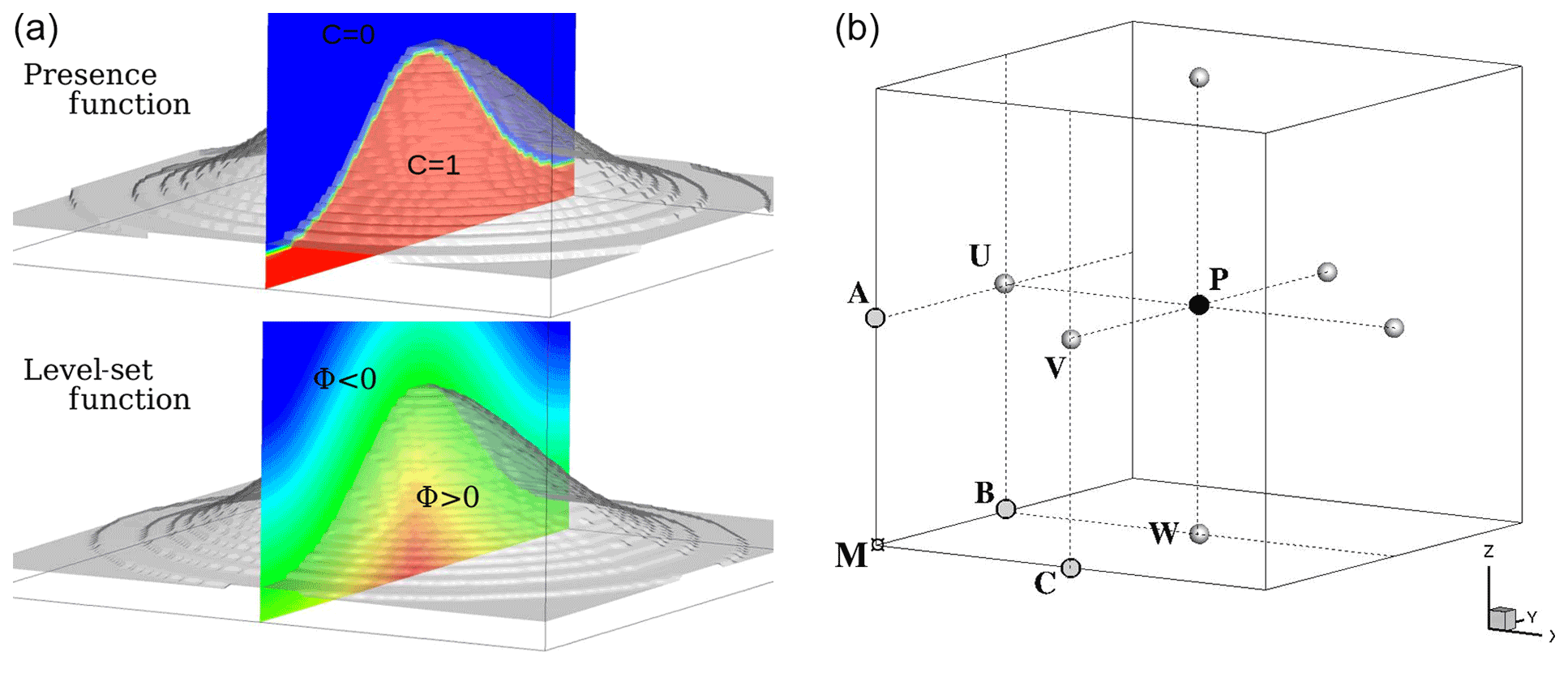
Figure 1(a) Illustration of two ways to model a fluid–solid interface: the color code indicates the isocontours of the presence function C and the level-set function ϕ. (b) Definition of the point types per cell: M is the geometric mesh point, P the mass point, the velocity nodes, and A, B, C the vorticity nodes.
3.1 Ghost-cell technique and explicit-in-time schemes
The ψn value is estimated at the time nΔt (Δt, the time step). The tendencies of the prognostic variables (Sect. 2.1) cannot be deduced from the conservation laws in the solid region. Expecting a correction due to IBM, wherein ϕ≥0, a general formulation of the tendencies is written as
The right-hand-side (RHS) first term of Eq. (10) is given by the conservation laws (Sect. 2.1). The tendency is the correction due to the GCT in the solid region and near the immersed interface, satisfying the desired boundary conditions at ϕ=0:
Note that is taken into account in the ERK temporal algorithm. The freeze of the immersed wind conditions in the ERK algorithm has also been implemented; it has shown more unstable behavior for a large Courant number.
The forced points are called ghost points and are renamed ghosts. To estimate the variable and for each ghost, the physical information is extracted near the interface and from the fluid region. The extension (grid stencil) of the forcing zone depends on the spatial accuracy of the numerical scheme. For example, Fig. 2b–c show the case of a two-layer stencil in a two-dimensional grid. The characterization of the layer is done by a conditional loop applied direction by direction on the LSF. For a 2-D case, the sign of and is estimated. The integer value kl determines the cells truncated by the interface: kl=1 (kl=2) defines the first (second) layer. The calculation of these ghost layers has a computational overhead due to data exchange among processors in parallel simulations. The stencil of the numerical scheme modeling the interface defines the kl value. In order to limit this overhead, a low-order version of a centered explicit-in-time scheme (Sect. 2.1) is employed when . The CPU cost of the “hybrid” advection scheme is largely compensated for by the decrease in the ghost number and parallel exchanges. Appendix B reports a comparison analysis between third-order weighted essentially non-oscillatory (WENO) and second-order centered schemes used in the vicinity of the interface; the studied case is the inviscid flow around a circular cylinder.

Figure 2(a) Node definitions acting in the ghost-cell technique: the ghost (G), interface (B), normal vector (n), mirror (I) and images (I1,I2). (b, c) Illustration of classical (new) GCT using the mirror (images). Triangles correspond to one of the node types (see Fig. 1b).
In classical GCT (Tseng and Ferziger, 2003) the fluid information is obtained at a mirror point (noted I, renamed mirror) found in the normal direction to the interface in such a way that the interface node B is equidistant to I and G. Figure 2a shows the characterization of one ghost G (of LSF value ϕG), its associated mirror I (of LSF value ϕI) and the interface node B (GI=2ϕGn). Figure 2b illustrates several ghosts and mirrors. The distance depends on the forcing stencil, and a problematic case regularly met in the mirror interpolation is the vicinity of ghosts with the interface (, with Δ the space step), leading to a not well-posed condition.
The new GCT. To overcome this problem, we define image points (noted I1 and I2 in Fig. 2a; renamed images) having a distance to the interface that depends only on the grid spacing: with . Figure 2a shows the images for one ghost. The new approach enforces a large enough value of the distance. Figure 2b (c) illustrates classical (new) GCT for several ghosts. Figure 2b shows some mirror points associated with ghosts of the first layer in the vicinity of the interface. Figure 2c shows that the new approach ensures the image points are always located in the fluid region, irrespective of the ghost location. The definition of several images per ghost allows us to build a profile of the fluid information normal to the interface. is therefore recovered by a quadratic reconstruction f using the points. Two distinct calculations of noted PLIa and PLIb are tested to build the Lagrangian interpolation:
where La(I) and Lb(I) are the Lagrangian polynomials, as follows.
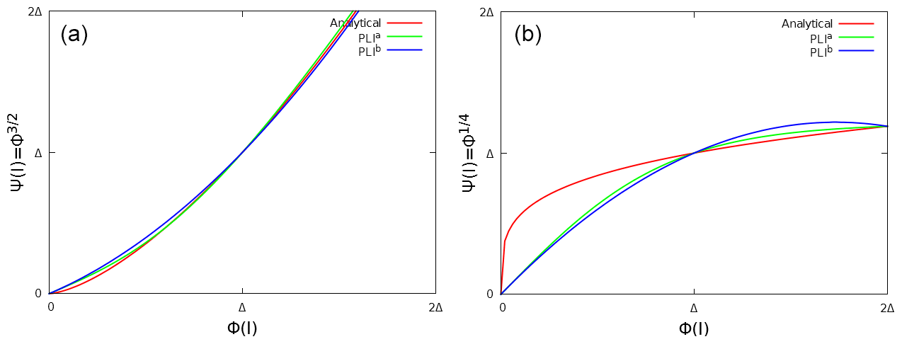
Figure 3Quadratic interpolations of two analytical profiles (red lines) using two image points at and the interface node. Green (blue) corresponds to La (Lb) polynomial results.
The accuracy of an interpolation depends on the profile. For example, a logarithmic evolution of the tangent velocity is expected in LES. Otherwise, when the viscous layer is modeled, a linear evolution is expected. To compare the ability of each quadratic interpolation to approach a wide variety of profiles, the recovery of power laws such as (Fig. 3a) and (Fig. 3b) is studied. As illustrated, PLIa fits the two analytical solutions better and is therefore adopted. The classical and new GCTs have been compared thoroughly, and part of this analysis is deferred to the Appendix. The interpolated field of the potential flow around a single cylinder or a sphere was compared to the theoretical solution; the sensitivity of the inviscid flow around the same bodies (Appendix B) to the type of GCTs has been studied. The new GCT has given the best results, especially in the symmetry preservation in the inviscid flow cases. Note that these results are also dependent on the 3-D interpolation choice detailed in the following paragraph. The proposed GCT is employed in the rest of this study. The GCT implementation is divided into four main steps: the fluid information recovery, the interface basis change, the interface condition and the ghost value.
The fluid information recovery. , for the images contained in a pure fluid cell (all corner nodes are in the fluid region), is recovered by a trilinear interpolation based on Lagrangian polynomials (LP), as follows.
For truncated cells (at least one corner node is in the solid region), is recovered using an inverse distance-weighting (DW) interpolation:
where (α=1). This formulation diverges when xi→xl and it is commonly adopted to impose when (ϵ is an arbitrary parameter depending on the mesh discretization, ϵ≪Δ). The 3-D extension is direct with . The use of these interpolations was decided after comparisons with barycentric Lagrangian and modified distance-weighting interpolations (Franke, 1982) and tests on the α coefficient. As the boundary condition is expressed in the interface frame and the grid is staggered, the non-collocation of the components implies the interpolation of three different classes of cells (with corners; Fig. 1b) for each ghost and building the change of frame matrix for which the proposed GCT presents an interest during the characterization of the direction tangent to the interface.
The interface basis change. Velocity vector , known in the Cartesian mesh basis at the images Il (Δn1=Δ and Δn2=2Δ in Fig. 2a), is projected in the basis of the interface in which the boundary conditions on each vector component are imposed. Computing the LSF gradient, the normal direction is defined. Otherwise, (t,c) represents two arbitrary tangent directions. The tangent direction t is considered the predominant tangent direction of the flow along the fluid–solid interface depending on the image values and defining the velocity vector as . The cotangent direction is defined as
The basis at the interface is defined by considering (or not) the rotation of the tangent velocity with the distance to the interface:
Finally, the third component is and (inverse) projection is known.
The interface condition. Let and be the Dirichlet and Neumann conditions on . The general formulation of the boundary condition is written as a Robin condition: ). The switch between the Dirichlet condition and the Neumann condition is done through the coefficient . To give some examples of a Dirichlet condition, is imposed on the velocity component normal to the interface arising from the impermeability hypothesis and on the component tangent to the interface for a no-slip hypothesis. To give some examples of the Neumann condition imposed by : a no-flux condition on the potential temperature (as well on a passive scalar, subgrid kinetic energy) and a free-slip case applied to . Note the approximation in the location of the derivative term and the Neumann condition depending on the chosen image (in practice the selected image Il is the closest one to the interface).
An interface condition depending on the characteristics of the surrounding fluid such as is a wall model. Using two (three) images, simple wall models such as the constant (linear) extrapolation of the gradient is reached by the () computation. The consistency between the tangent component to the interface of the resolved wind and the subgrid turbulence is the subject of Sect. 2.3.
The ghost value. Knowing and , ψ(G) for a Dirichlet (Neumann) condition is written as
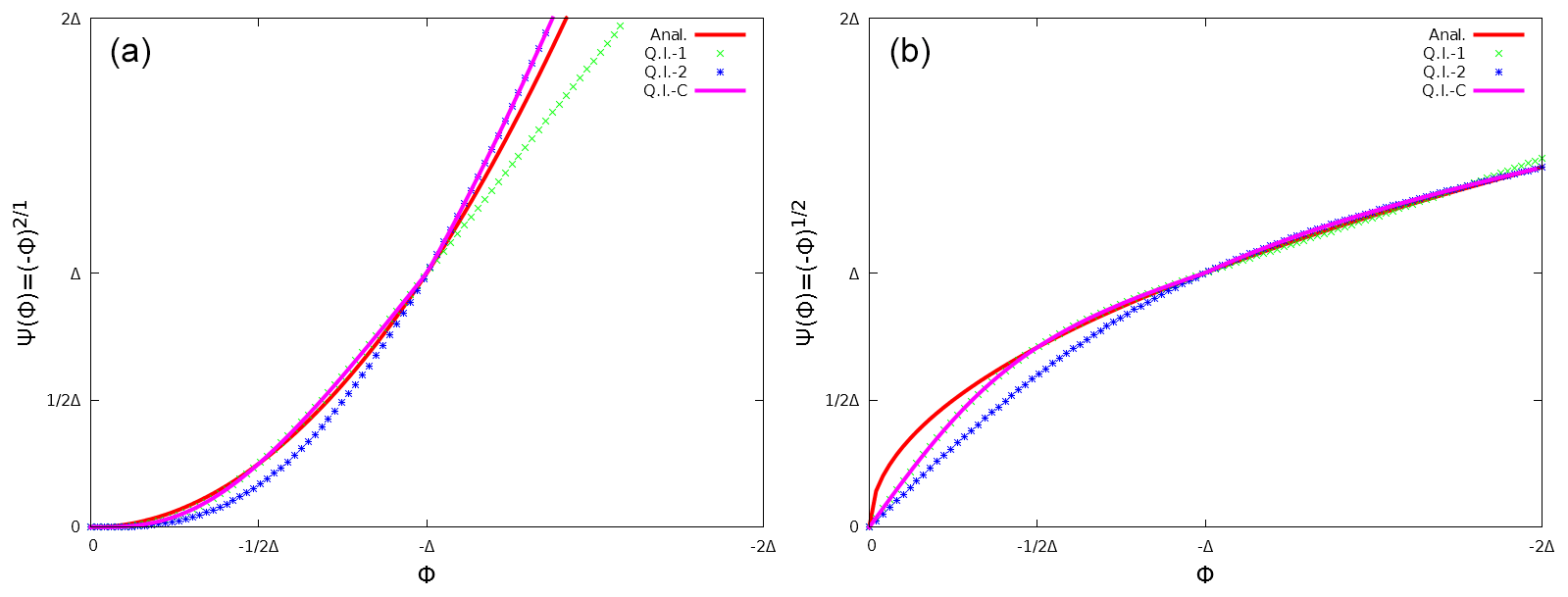
Figure 4Profile normal to the interface of two points of fluid information : analytical solution (red lines), quadratic interpolation QI1 using (green symbols), QI2 using (blue symbols), QIC as a combination of QI1 and QI2 (purple lines).
In practice, three Il images are defined for which the locations are with . The choice of the image distance to the interface affects the results. To best approach the expected solution, two quadratic interpolations depending on the images used and one combination of these quadratic interpolations are tested. Figure 4a and b illustrate these interpolations by considering two analytical profiles (red lines): the quadratic interpolation QI1 (QI2) is based on the image values located at and ϕ=Δ and plotted in green symbols (at ϕ=Δ and ϕ=2Δ plotted in blue symbols). Depending on the analytical profile, Fig. 4 shows the influence of the image location choice. As expected, QI1 (QI2) appears to be less accurate than QI2 (QI1) for (for ). QIC is the combination of QI1 and QI2 (purple line). QIC preserves the advantage of each quadratic interpolation and when ϕG<Δ (ϕG>Δ), QI1 (QI2) is used in the rest of the study. Knowing at the end of the MNH temporal loop with QIC, the profile is extrapolated from the fluid region to the solid region by applying an anti-symmetry . The ghost value is estimated and the gradient at the interface is also recovered.
3.2 Cut-cell technique and pressure solver
First looking at the RHS of Eq. (5), the coming from the resolution of the explicit-in-time schemes near the interface and in the solid regions badly affects the computation (note that the GCT operates after the step projection). Therefore, the fictive wind of the solid region can spread errors in the fluid region during the pressure resolution. To avoid it, a correction of the pressure solver is proposed.
The elliptic problem (Eq. 5) is rewritten as a resolution of the linear system . In the standard MNH version, is estimated using a finite-difference approach. To uncouple the solid region from the fluid region our revisited version enforces a null divergence for pure solid cells and estimates the balance of momentum fluxes by a finite-volume approach for truncated cells (noted 𝒬cct):
where 𝒱=Δ3 is the cell volume, 𝒱f (𝒱s) the fluid (solid) part of 𝒱 and 𝒮i the cell surfaces for which i is the index of each surface orientation [e, w, n, s, b, f] as illustrated in Fig. 5a.
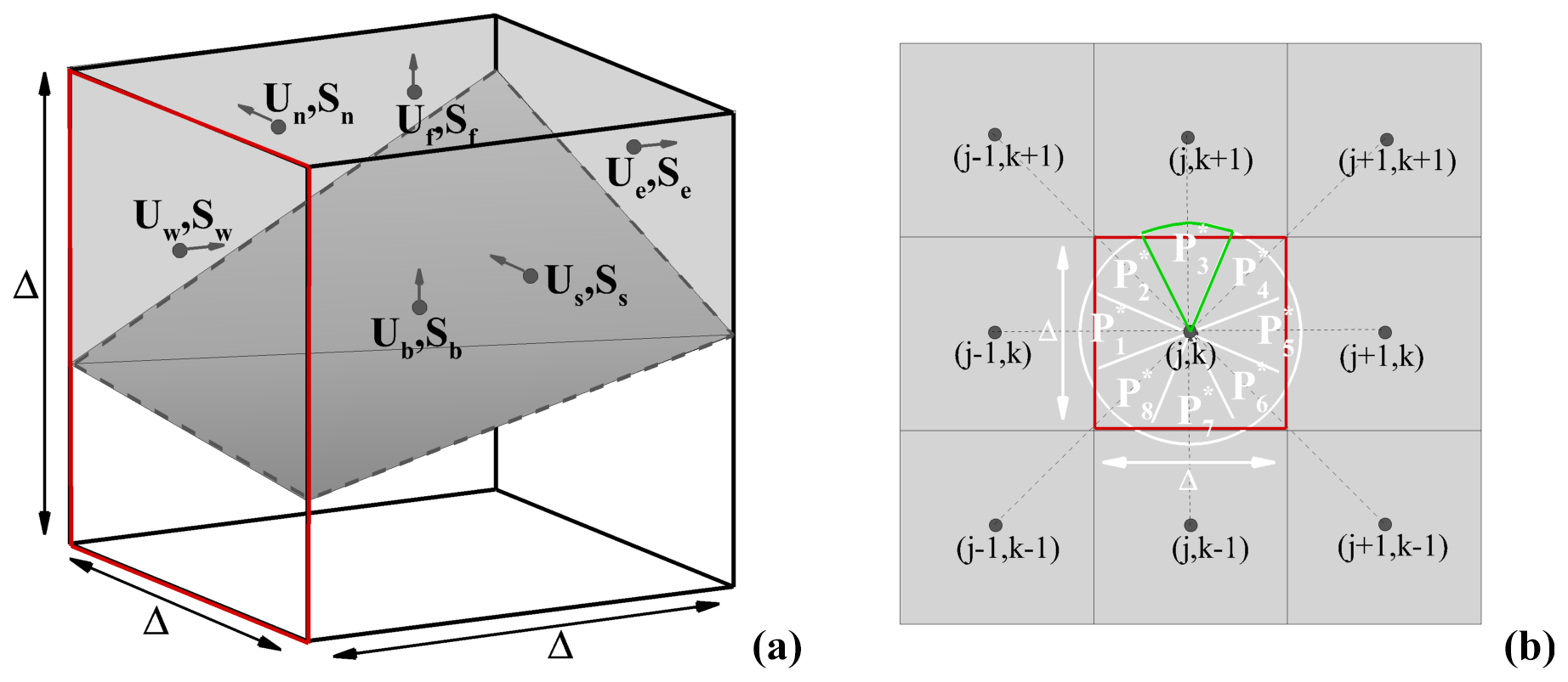
Figure 5(a) Momentum flux balance for an arbitrary truncated cell of volume 𝒱, where the velocities (Ui in the figure, ) are supported by the 𝒮i surfaces in grey; the transparent volume is a part of the solid body. (b) Segmentation of the 𝒮w arbitrary surface (red border) in eight pieces of cake (the border of is indicated in green).
According to the Green–Ostrogradski theorem, the calculation is the classical way of a CCT (Yang et al., 1997; Kim et al., 2001) to estimate the velocity divergence. A similar approach is performed here by rebuilding the flux for truncated and solid cells.
The calculation consists of a weighting of the outflux and influx function of the fluid and cell surface ratios (Fig. 5a). Figure 5b gives an example of the west surface (i=w, red border) in which is calculated using the LSF value ϕ=ϕw and the ones of the eight adjacent nodes . A disk of radius is split into eight “piece-of-cake” segments (). An LSF linear interpolation detects (or not) the interface location. In the presence of an interface, its distance from the studied node is . Knowing δp, the momentum flux balance is formulated for a nonmoving body as (p is the index of the piece of cake and i the index of the cell surface)
The four encountered cases correspond to a pure fluid cell when ϕp<0 and ϕi<0 (Fig. 6a); a pure solid cell when ϕp>0 and ϕi>0 (Fig. 6b); and two types of truncated cells depending on the fluid–solid nature of the main node for which (Fig. 6c–d). Using Eq. (23), Eq. (22) is solved and leads to the RHS computation of Eq. (5).

Figure 6(a–d) calculations depending on the signs of ϕi=(ϕ) and ϕp on an arbitrary piece of cake. The white (grey) region corresponds to the solid (fluid) one of (same color code as in Fig. 5).
Knowing 𝒬cct, the reflection now concerns the 𝒫 matrix to invert. The classical interface condition on the potential Ψ∗ is a homogeneous Neumann condition . Using a boundary-fitted method (BFM), the interface condition of the moving or nonmoving body (Auguste, 2010) appears only on the border of a numerical domain. Using an IBM and without any impact of this interface condition on the 𝒫 coefficients, the impermeability character of solid obstacles is not achieved. Due to the inversion of the horizontal part of 𝒫 by a fast Fourier transform (Schumann and Sweet, 1988), the solution of calculating 𝒫cct appears to be problematic. The adopted solution consists of an iterative procedure as used in MNH for non-flat problems. The non-respect of the Ψ∗ condition in 𝒫 leads to a not well-posed system, and the iterative procedure spreads to the entire fluid domain the enforcement of the null divergence imposed on solid cells. The resolution of the pseudo-Poisson Eq. (5) leads to , where M is the number of iterations. This number is limited by a convergence criterion (compromise between incompressibility satisfaction and CPU cost). Many iterative procedures are available in MNH originally developed for non-Cartesian grids. Richardson and preconditioned conjugate residual algorithms have been adapted here to the obstacle immersion. The newly modified pressure solver is tested and validated in Sect. 4.1.
3.3 Consistency with the turbulence scheme
It is known that is a reasonable approximation in nonhomogeneous, non-isotropic turbulence such as in the near-wall region. This approximation is indeed retained in the present IBM implementation, which assumes lm=lϵ (hereafter noted lm and called the mixing length). The Redelsperger et al. (2001) corrections near the ground are to match the similarity laws and the free-stream model constants are not activated. lm is equal to the numerical cutoff space scale sufficiently far from the ground, leading to a turbulent viscosity. Near the ground and following the Prandtl idea consisting of the assumption of the linear variation of lm in the near-wall region, the upper limit of the mixing length is (k is the von Kármán constant and z is the altitude).
The turbulent characteristics are highly affected by surface interaction. As a consequence and for LES, the subgrid turbulence scheme (Sect. 2.3) is modified in the presence of immersed obstacles in the subgrid turbulent kinetic energy equation (Eq. 6), mixing length computation and Reynolds stress diagnosis (Eqs. 7, 8 and 9).
The subgrid turbulent kinetic energy condition. The explicit-in-time resolution of Eq. (6) claims a GCT forcing and an interface condition on the STKE e. Commonly, the STKE profile is considered parabolically in the viscous sublayer (Craft et al., 2002; Bredberg, 2000) and constant in the inertial and wake outer layers (Kalitzin et al., 2005; Capizzano, 2011). Due to the high turbulent Reynolds number encountered, a homogeneous Neumann condition is applied at the immersed interface. The equilibrium between the production and dissipation of STKE could be discussed and controverted; this choice acts as a first stage in IBM development.
The near-wall correction of the mixing length. The von Kármán limitation due to immersed walls acts through the LSF, and the upper limit on the mixing length lm near the interface becomes with a banning of negative values in the solid region. Whatever the production of STKE and the turbulent shear, the lower limit induces a null value of the diagnosed surface fluxes. In addition, a singularity appears in the dissipative term . Through pragmatic reasoning, the singularity due to amounts to the modeled length scales being smaller than the Kolmogorov scale (ν3ϵ−1)¼. Considering the Kolmogorov scale as modeled, the turbulence should vanish, which is in contradiction to the dissipative term. In order to overcome this ill-posed problem, a lm lower limit has to be specified. In the study of atmospheric flows around buildings, a characteristic thickness of the viscous layer can be defined around an H bluff body for a Reynolds number based on the obstacle scale: H≈𝒪(10m); Re≈𝒪(107). This thickness estimate is also proportional to (E≈9.8 is commonly employed), whereby the friction velocity u∗ is about 1 cm per second. Following these estimates, the length scale due to the viscous effects belongs to the millimeter domain in the expected atmospheric cases. Looking after a building surface and its large heterogeneity (door, windows, surface characteristics), its roughness length is at least in the decimeter domain and (Illustration in Fig. 7). For low Re and smooth surfaces, could be encountered. Therefore, we assume and that zib is related to the size of smallest unresolved eddies near walls (i.e., dissipative scale). The mixing length near the wall is .
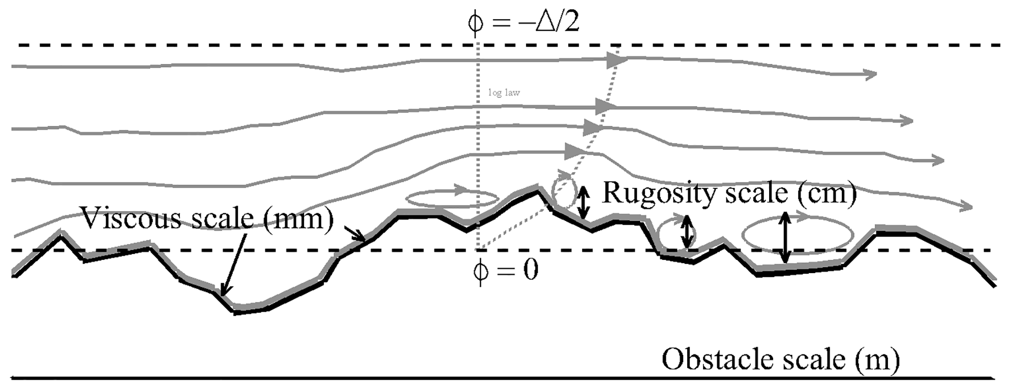
Figure 7Illustration of the unresolved physical processes near a nonidealized solid wall (black line) in an atmospheric context: the length scale based on the viscous effects (grey line) is drastically smaller than the roughness length. The roughness length approaches the scale of smallest eddies and governs the log-law profile.
The turbulent fluxes correction. The gradient and the turbulent diffusion prescribe the turbulent fluxes at the immersed interfaces (Eqs. 7, 8 and 9). As a first step in the MNH–IBM implementation, a no-flux condition on the mean potential temperature is imposed, leading to a zero value of the sensible heat flux. Writing the mean velocity field at B as , is needed to recover a gradient consistent with the turbulent shear. Considering the Prandtl (1925) or von Kármán (1930) theories, the logarithmic profile is assumed in the vicinity of the wall according to . Considering Δ to be the limit of the resolved scales, most of the turbulent kinetic energy is contained in the subgrid when and as with a constant Ktke≳1. This assumption is reinforced by the homogeneous Neumann condition applied on e. This approach derives from RANS (Reynolds-averaged Navier–Stokes) approaches, and the velocity friction is formulated as , where Cμ is a constant evolving between 0.03 (atmospheric applications) and 0.09 (fluid mechanics applications). Adding a damping function for the viscous cases (low turbulent Reynolds number, Ret<20), the tangent wall velocity at the interface is written as
Finally, the pragmatic limitation operates if the STKE value is too high. The proposed dynamic wall model evolves between the no-slip and free-slip conditions. If the subgrid turbulence is weak or if the physical problem is fully resolved, the viscous layer is well modeled and . Otherwise, for an intense subgrid turbulence or a fully unresolved problem, the shear due to the wall presence is not perceived and . The wall model establishes an equilibrium between the production of STKE and the mean parietal friction. Note that the use of a log-law model near a singularity such as sharp edges and corners could be called into question. Nevertheless, Section 5.1 and 5.2 show LES results employing this proposition. After numerical investigations done during the single-cube study, appears to be a suitable choice.
4.1 Potential flow
Isolated from the rest of the code, the resolution of the pseudo-Poisson Eq. (5) leads to potential solutions (Sect. 2.2). Theoretical ones are available for flow developed around a nondeformable obstacle such as an infinite cylinder or a sphere (Milne-Thomson, 1968; Batchelor, 2000). The two bodies are investigated here. The flow around the infinite cylinder is predominantly presented.
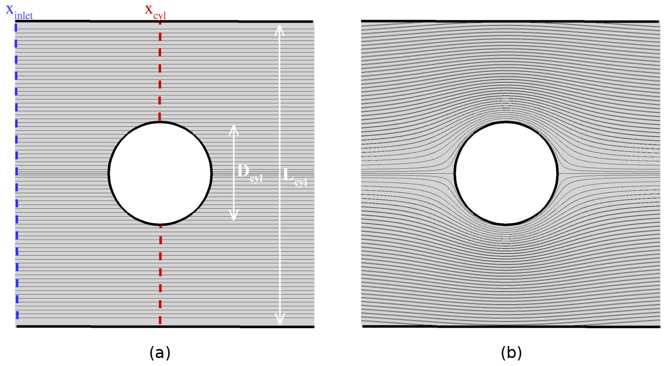
Figure 8Potential flow around a cylinder: (a) initial state around the body of diameter Dcyl=2Rcyl; (b) streamlines obtained after the Poisson equation resolution. The confinement is defined as ).
Figure 8 illustrates the cylinder case. The fluid density is considered constant in time and in space. The flow is initially imposed as spatially homogeneous with a constant module of velocity U∞ and parallel streamlines (Fig. 8a). This initialization does not respect the conservation of the momentum flux, and the irrotational correction of the projection method goes to recover this conservation. At the same time, the impermeability of the cylinder of diameter Dcyl=2Rcyl is achieved. Figure 8b shows the streamlines obtained with the MNH pressure solver modified to take into account the presence of immersed obstacles (Sect. 3.2). Defining x as the direction parallel to the initial streamlines and y as the perpendicular one, the expected solution is (single and non-confined body, (α;r) cylindrical coordinates). The numerical confinement is discussed hereafter, characterized by , where Lcyl is the distance separating the lateral domain surfaces (Fig. 8a).
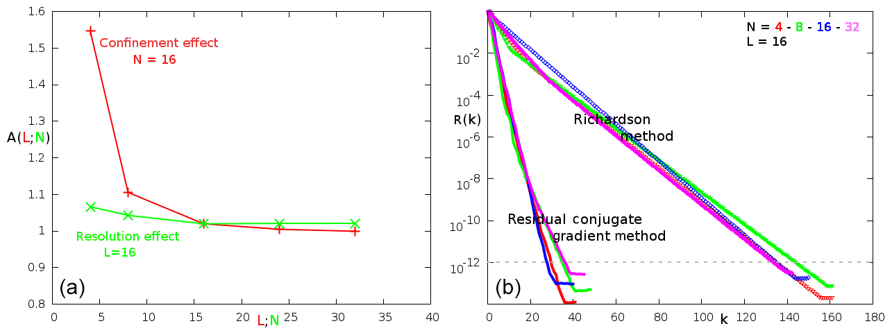
Figure 9Potential flow around a cylinder: (a) velocity convergence of two iterative methods (residual conjugate gradient, Richardson) for different spatial resolutions (L=16); (b) evolution of the added mass coefficient A(N;L) with the confinement (N=16) and with the node number per radius cylinder N (L=16). The confinement is defined in Fig. 9a.
The Richardson (RICH) and the residual conjugate gradient iterative (RESI) methods are tested (Sect. 3.2). Figure 9a plots the evolution of the dimensionless residue R(k) (based on a characteristic divergence U∞∕Δ) with the iteration number k and obtained with the confinement L=16. The two algorithms converge with a weak dependence on the spatial discretizations ( nodes per Rcyl). The slope coefficient , so RESI demonstrates the highest velocity convergence. Even if RICH is about 20 % faster per iteration than RESI, the global CPU cost of the last one is lowest for the same solver residue R(k). For this reason and due to a higher a priori radius convergence, RESI is adopted. Note that the momentum flux computed after the solver convergence at the xcyl location (Fig. 8a) shows good mass preservation with a relative error of in regard to the incoming flux localized by its xinlet longitudinal coordinate. Similar results were obtained with a spherical body (not shown here).
With a change of Galilean reference frame, this study corresponds to a uniform body acceleration ab in a fluid initially at rest. However, a possible viscous term, the hydrodynamic force exerted on the body, is reduced to the added mass effect for Δt→0. 𝒜 is the dimensionless coefficient and mf the displaced fluid mass. 𝒜cyl theoretically equals 1 in the non-confined cylinder case (Lamb, 1932). The red curve in Fig. 9b illustrates the effect of the confinement L on 𝒜cyl for N=16 resolution. Unsurprisingly, 𝒜cyl increases with the confinement (Brennen, 1982). The weak dependence of 𝒜cyl with L>16 allows us to consider the body to be isolated for L∼16. The green curve in Fig. 9b shows the impact of the space resolution for L=16. The numerical added mass coefficient is in good agreement with the theoretical one, presenting a relative error of about 2 % for N>16. It induces a respect for the impermeability hypothesis at the immersed interface. A similar study for a spherical body gives . Figure 10 illustrates the contours of the kinetic energy around the sphere in an arbitrary symmetry plane. The green contours (numerical solutions) fit well with the red contours (theoretical solutions). A convergence study of the pressure solver is discussed in Appendix A.
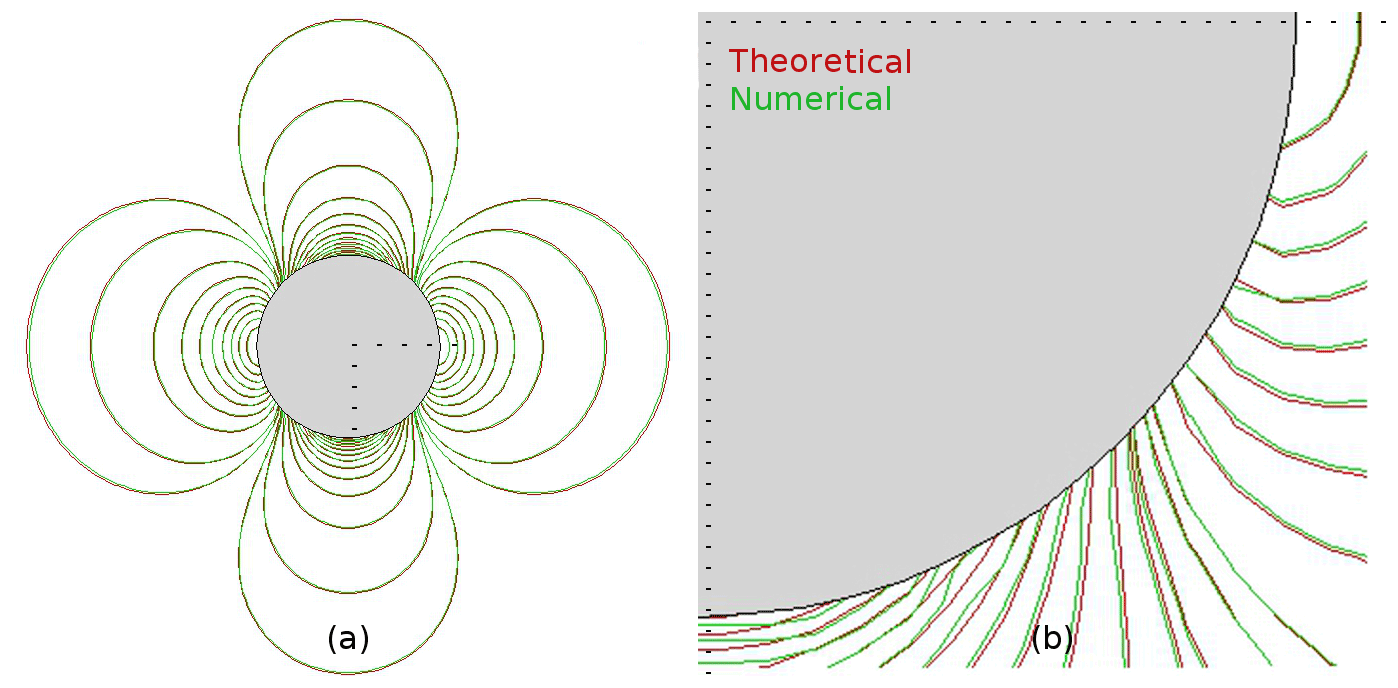
Figure 10Potential solution around a sphere: (a) kinetic energy in an arbitrary symmetry plane; (b) zoom.
4.2 Viscous flow
A pure dynamic and well-documented case that naturally follows previous ones is studied here. This physical case is the wake past a circular cylinder (non-stratified flow) at two moderate Reynolds numbers . One of the forerunners is Taneda (1956), who experimentally studied the nature of eddy structures.
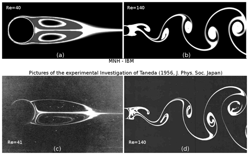
Figure 11Eddy structure in a viscous fluid: steady (left, Re≈40) and unsteady (right, Re≈140) solutions obtained by the current numerical investigation (a and b, MNH–IBM and 30pts∕Dcyl) and by the Taneda (1956) experiments (c and d). The visualization is due to the presence of a passive tracer injected on the body surface and transported by the flow.
Taneda (1956) found a regular Hopf bifurcation at a critical Reynolds number . Below Rec and above Re>5, a boundary layer separation leads to a steady recirculating region in the near wake (Fig. 11c). Above Rec≈45, an unsteady mode breaks the planar symmetry and the body wake presents an alternate vortex shedding (Fig. 11-d). The standing eddy (the von Kármán street) obtained by MNH–IBM at Re=40 (140) is visualized in Fig. 11a (b) by the injection of a passive tracer on the body surface.
The standing eddies at Re<Rec are commonly described with a θd detachment angle, lr recirculating length and (a;b) location of the vortex core (Fig. 12). The limit of the numerical domain is 10Dcyl upstream of the obstacle for the inlet condition (U∞, the uniform incoming velocity) and lateral condition (slip condition) and 15Dcyl for the outlet condition, allowing for the vorticity evacuation. As Cai et al. (2017) mention, this domain can induce a low numerical confinement effect. Three regular Cartesian meshes are built with 10, 20 and 30 nodes per Dcyl.
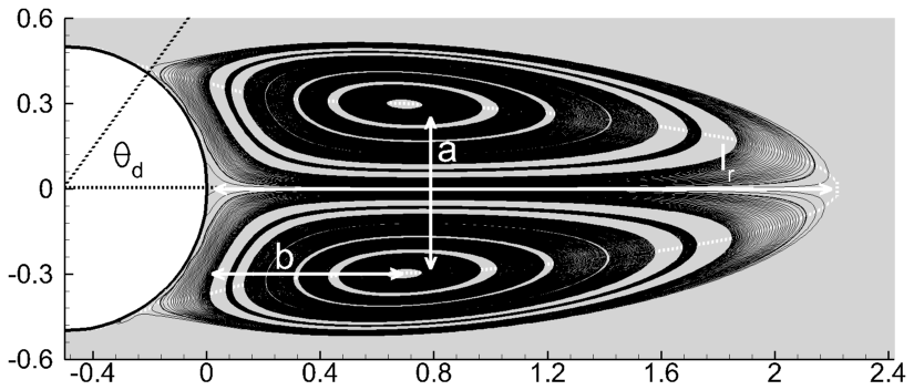
Figure 12Recirculating region at Re=40 (MNH–IBM, 20pts∕Dcyl): definition of the θd (∘) separation angle, lr recirculating length and (a;b) vortex core location. The distance is dimensionless by Dcyl.
The 20pts∕Dcyl and 30pts∕Dcyl meshes present a good spatial convergence and weak differences at Re=40. and the recirculation length . The 10pts∕Dcyl mesh shows more discrepancies, which are attributable to the nonability of the coarsest resolution to capture the viscous boundary layer for which the thickness evolves in . Note that the impact of the low-order (centered or WENO) modeling of the advection at the immersed interface is weak for this viscous case (Sect. 3.1). Table 1 compares the 20pts∕Dcyl results with a part of the results literature collected in Gautier et al. (2013).
Coutanceau and Bouard (1977)Linnick and Fasel (2005)Taira and Colonius (2007)Bouchon et al. (2012)Gautier et al. (2013)Cai et al. (2017)Table 1Description of the standing eddies in the wake of the solid cylinder (Re=40): comparison of the separation angle θd (∘), recirculating length lr (m) and vortex core location (a;b) between the literature and MNH–IBM.

The focus is on the unsteady mode at Re=140. The ratio between the characteristic time of inertial effects Dcyl∕U∞ and the one related to the vortex shedding 1∕f defines the Strouhal number . Brazza et al. (1986), Park et al. (1998) and Stålberg et al. (2006) confirm the equation proposed by Williamson (1989). MNH–IBM obtains and an absolute maximum relative error lower than 2 % in regard to the Williamson (1989) formulation with the two finer resolutions. Our results are in good agreement with those presented in the abovementioned and more extensive studies. Details on DNS validation in a viscous buoyancy-driven flow are also presented in the Supplement.
This section is devoted to turbulent flows approaching our perspective: the simulation of an atmospheric flow over a city. The turbulent flows around a cubic body vertically confined in a channel and over an urban-like roughness (set of obstacles) are here described. MNH–IBM is explicitly compared to experimental investigations in the two cases. Comparisons to other LESs from the literature will be mentioned.
Common hypothesis and methods. The fluid is considered as neutrally stratified. The Coriolis term is negligible due to the addressed space scales and timescales. The turbulent diffusion is modeled by the subgrid TKE1.5 scheme transported by PPM (Sect. 2.3). All surfaces are considered non-permeable and the IBM wall model (Sect. 3.3) is activated. An reference frame is defined (z, vertical direction) and the velocity vector is written as . A time simulation is needed afterwards to establish the turbulence state (not shown here). The overline notation refers to the mean value in time in this section.
5.1 Flow over a surface-mounted cube
Using static pressure measurements, as well as laser-sheet and oil-film visualizations, Martinuzzi and Tropea (1993) and Hussein and Martinuzzi (1996) generated a large data set for the study of flows around a cubic body placed in a channel (Fig. 13a). RANS and LES have been used to explore in detail this physical case (Breuer et al., 1996; Shah and Ferziger, 1997; Rodi et al., 1997; Frank, 1999; Krajnovic and Davidson, 2002; Farhadi and Rahnama, 2006).
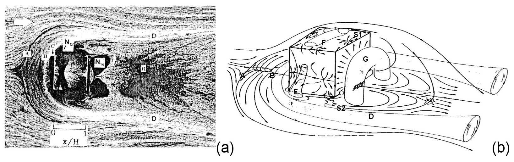
Figure 13(a) Top visualization of the flow around a cube (Hussein and Martinuzzi, 1996); (b) schematic representation of the time-averaged vortex structure around a cube (Martinuzzi and Tropea, 1993) and index of the recirculating regions.
Physical details. A cube (H side) is placed in a channel of 2H height. The channel is sufficiently large in the spanwise direction to consider the cube to be single in that direction. Turbulent flow is generated in the channel upstream of the cube with a mean bulk velocity Ub. Defining the dimensionless wall coordinate , the stream-wise upstream velocity corresponds to a log law for smooth walls as described in Hussein and Martinuzzi (1996). The Reynolds number, as defined by the mean bulk velocity, the cube height and the molecular diffusion, is Re≈40 000.
The mean flow around the cube presents a set of five recirculating regions (Fig. 13b). Each cube surface is associated with one of these regions: the A–B vortex separations in front of the cube, which spread laterally in a horseshoe D, two vortices near side walls E, one F on the roof and main arch vortex G downstream.
Numerical details. The top and bottom surfaces of the cubic body are modeled by the IBM. A small value of the roughness length is imposed (low value to model a smooth interface, viscous-scale intervention in the z+ calculation). The stream-wise (spanwise) direction is x (y). The size of the grid is set as with a location of the cube center at . Three regular Cartesian meshes are employed with a respective space step . is a region employed to model the fully turbulent character of the incoming flow. The incoming turbulent state is obtained by the IBM and a pseudo-recycling method inspired from the works of Lund (1998), Mayor et al. (2002), and Yang and Meneveau (2016) (not detailed here). The vertical profiles of the stream-wise velocity and turbulent intensity (Hussein and Martinuzzi, 1996) are recovered at . We note that the turbulence generation deserves more attention, but we prefer to concentrate only on the cube wake.
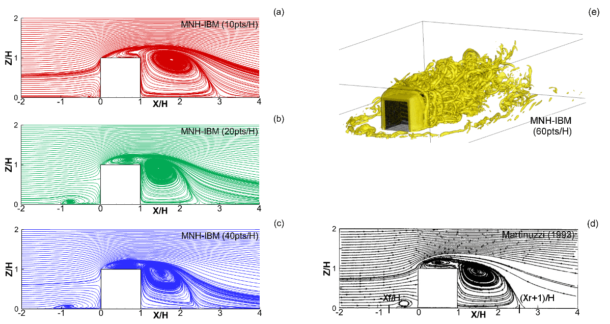
Figure 14Vertical symmetry plane of the mean flow: (a–c) MNH–IBM time-averaged streamlines; (d) streamlines observed by Martinuzzi and Tropea (1993); (e) MNH–IBM instantaneous visualization of the Q criterion (Hunt et al., 1988).
Results. Figure 14a, b and c show the time-averaged streamlines in the vertical symmetry plane of the cube obtained by MNH–IBM for the three space resolutions. The streamlines of the coarse, medium and fine resolution are respectively in red, green and blue. The discretization order of the fine resolution is close to that of most literature LESs except Shah and Ferziger (1997), who used a far more precise grid near walls. The same figure obtained by the experimental investigation is given in Fig. 14d. The size of the front (rear) region is characterized by the recirculating length xf∕H (xr∕H). The experiment gives and . The LES reference results give the ranges and . For the two finest resolutions (green and blue), the overall prediction of MNH–IBM recovers a consistent mean topological structure. MNH–IBM obtains for the two finest resolutions and . MNH–IBM does not capture, as with most LESs, the two dividing lines A∕B mentioned by Martinuzzi and Tropea (1993) but only captures a flattened vortex. However, the bifurcation point near the rear edge and ground is not detected by MNH–IBM, while this point was modeled in Rodi et al. (1997). This bifurcation point was also commented on in Martinuzzi and Tropea (1993), even if their experimental uncertainty did not allow us to visualize it in Fig. 14d.
Figure 14e shows an MNH–IBM instantaneous flow field with the Q criterion (Hunt et al., 1988), and as the LES reference results mention, it presents a highly intermittent character clearly visible with the quasi-disappearance of the D horseshoe and G arch. A frequency f of vortex shedding dominates the highly intermittent activity in the body wake, leading to the experimental Strouhal number . An MNH–IBM energy spectrum (discrete Fourier transform of w(t) in the body wake) finds a peak for all the studied resolutions and a energetic cascade slope for larger wave numbers (not shown). The St values obtained by MNH–IBM are slightly lower than the experimental one but stay consistent with the range of other LESs.
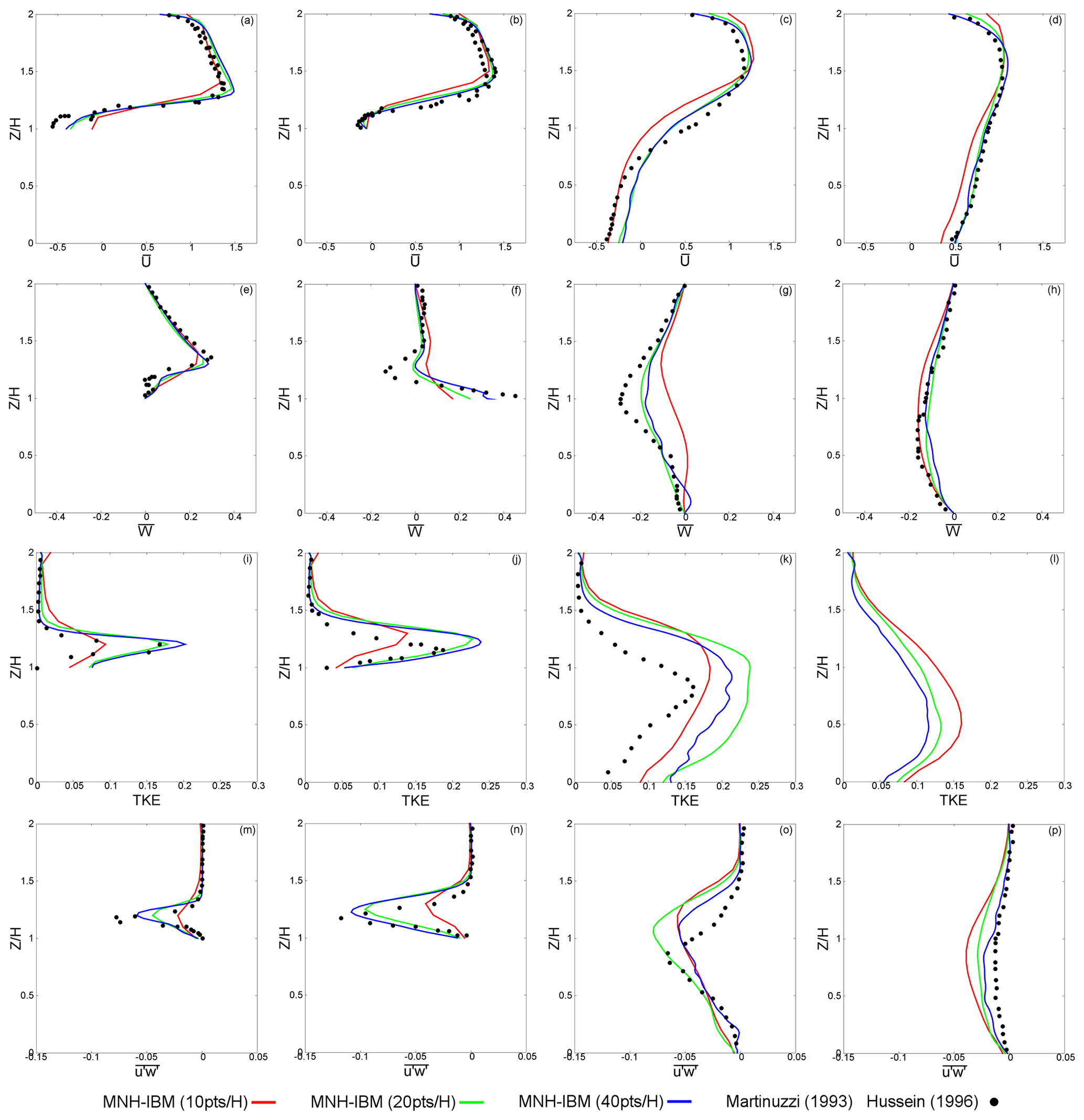
Figure 15Mean vertical profiles of velocities (top), turbulent kinetic energy and Reynolds stress (bottom). The lines correspond to the MNH–IBM results. The symbols are the Martinuzzi and Tropea (1993) data except for TKE (Hussein and Martinuzzi, 1996). The profiles are given at four longitudinal locations: (a, e, i, m) ; (b, f, j, n) ; (c, g, k, o) ; (d, h, l, p) .
Still in the vertical symmetry plane of the mean flow, Fig. 15 plots at four longitudinal positions the vertical profiles of time-averaged quantities related to the steady (, ) and unsteady (TKE, ) parts of the solution. The color code corresponds to the spatial resolution (10pts∕H in red; 20pts∕H in green; 40pts∕H in blue). Note that the Ub bulk velocity was set to unity and therefore presents variables in Fig. 15 that are dimensionless. In most of the sub-figures, the higher the space resolution, the lower the gap with the experiment. The top of Fig. 15 leads to a similar conclusion as the literature LESs: the stream-wise velocity is well recovered. The counterflow at the rear and roof of the cube near informs us about the existence of the bifurcation point S1 (Fig. 15b). An underestimation appears on the counterflow at and is frequently observed in the literature (Fig. 15c). Some discrepancies are found on two profiles (Fig. 15f–g). Note that Shah and Ferziger (1997) and Krajnovic and Davidson (2002) highlight the difficulty of recovering it. The turbulent kinetic energy and the Reynolds stress are correctly predicted at the cube roof (Fig. 15i–j). The vertical profiles of TKE and downstream of the cube show an overestimate tendency (Fig. 15k, p, l). No experimental data are available on TKE at (Fig. 15l), but using the experimental value (not shown here) and the ratio obtained by MNH–IBM, we suspect that TKE is still overestimated. This turbulence diagnosis is relatively similar to that of Farhadi and Rahnama (2006).
Sensitivity study. Some tests have shown a sensitivity of the solution with both the incoming turbulence and constants in the immersed wall model. Indeed, the existence of the small vortex near the saddle node S1 (Depardon et al., 2006) turns out to be strongly dependent on the inlet turbulence (the lower the turbulent intensity, the bigger the size of this vortex); the reattachment (or not) of the roof vortex F with the main arch G is also observed. This sensitivity follows the observations of Castro and Robins (1977), who studied the cube placed in a uniform or turbulent incoming flow. In the same way the existence of the vortex near the saddle node S2 (Frank, 1999) is dependent on the ground boundary condition. The ratio and the z0 roughness length fixed in the immersed wall model (Sect. 3.3) impact the nature of the incoming turbulent state for which the surface shear plays an important role. To give a significant example and if a null value of Ktke is applied on the channel surfaces (non-slip condition), xf highly increases and the vortex at S2 appears. Otherwise, Ktke and z0 do not crucially affect the nature of the dynamic in the vicinity of the cube surfaces; the pressure gradient between front and back faces governs.
To conclude this section and despite the uncertainties of the inlet condition, MNH–IBM is in good agreement with the experiments of Martinuzzi and Tropea (1993), Hussein and Martinuzzi (1996), and other LESs using a resolution of about 10 points per cube length. Even if the coarsest resolution loses a part of the expected physics, it maintains a suitable modeling of the largest structures of the flow. A parametric study on inlet turbulence generation has led us to fix Ktke≈2 in Eq. (24).
5.2 The Mock Urban Setting Test (MUST) experiment
The MUST is an experimental campaign organized during early autumn 2001 in Utah's West Desert (Biltoft, 2001; Biltoft et al., 2002). Its objective was to quantify the dispersion of a passive tracer (propylene) in a dry atmospheric context over a topography reproducing a near-urban canopy. The main interest lies in the similitude between this experiment and a pollution episode due to toxic gas propagation over a city with high population densities. It provides extensive measurements of meteorological variables and scalar dispersion information.
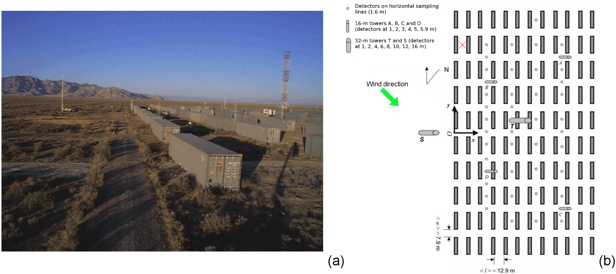
Figure 16(a) Photograph of the MUST containers in Utah's West Desert; (b) schematic representation of the container layout. The locations of the concentration (detectors) and wind sensors (S and T towers) are indicated, as are the position (red cross) of the pollutant release and the direction of the incoming flow (green arrow) for case 2681829. Source: Biltoft (2001) and Yee and Biltoft (2004).
Physical details. The near-regular array is composed of 120 containers. Figure 16 gives a photograph and a picture of the topography. The containers are equivalent in volume and shape. Their spatial dimensions are m and the horizontal distance between containers is 𝒪(10) m. Following Table II in Yee and Biltoft (2004), the 2681829 case (25 September 2001 at 18:29 UTC) is selected. The Monin–Obukhov length is Lmo≈28 000 m and the stability condition is supposed neutral; the buoyancy effects and the sensible heat flux are negligible in regard to the inertia effects and the turbulent shear. The incoming flow shows a mean horizontal angle with the container layout (green arrow, Fig. 16b). The MNH–IBM results are compared to the experimental measurements reachable at several altitudes (4, 8, 16 m) at the south tower and at the main T tower placed in the array center. The locations of the towers are indicated in Fig. 16b. A roughness length z0=0.045 m is given by the experiment and related to the surrounding desert vegetation.
Numerical details. The externalized scheme SURFEX (Masson et al., 2013) models the ground friction. LSF is generated to represent the topography and IBM is used to model the containers. The smallest characteristic container length is discretized by 𝒪(10) cells. The mesh is a Cartesian and regular grid for z<10 m with a space step Δ=0.2 m. Above 10 m, the vertical space step is released in a geometric progression of 1.08 ratio. The altitude of the numerical domain top is about 8 times the container height.

Figure 17Mean vertical profiles in the MUST experiment: (a) horizontal velocity; (b) wind direction at the S (blue) and T (black) towers. The symbols (lines) are the Yee and Biltoft (2004) experimental measurements (MNH–IBM results).
The distance between the horizontal limit of the computational domain and the array is about 20 times the container height. The large-scale flow is forced by an open boundary condition. A mean horizontal angle of −41∘ with the x direction is fixed for all altitudes; note that the low angle deviation and the turbulence observed upstream of the containers in the experiment are not numerically considered. Following the experimental data given at the S tower (Fig. 17a, blue symbols) and assuming a log law , a least-squares regression estimates a friction velocity m s−1 and allows us to build the vertical profile of the mean incoming flow (Fig. 17a, blue line). This u∗ value is close to the experimental one m s−1 found by a sonic anemometer at the feet of the S tower. The same inlet condition is used in the numerical studies of Hanna et al. (2004), Milliez and Carissimo (2007), and Donnelly et al. (2009). Note that an additional term appears in their formulation but is negligible in the 2681829 case.
Results. The black line (MNH–IBM) and symbols (Yee and Biltoft, 2004) in Figure 17a (b) show the impact of the near-urban canopy on the vertical profile of (wind angle) in the core of the array (T tower). Not surprisingly, the canopy induces a global slowdown of near the ground and up to z≲8 m. A decrease in the mean horizontal wind angle is found at the same altitudes. This deviation is related to the container orientation, which tends toward the flow being aligned with the y direction. The same pattern is discussed in Milliez and Carissimo (2007). A wind acceleration and an increase in the wind angle are observed by MNH–IBM for z≳8 m as in the LES results of König (2014) and Dejoan et al. (2010) on similar MUST cases. These few degrees of deviation are observed by the experiment but not the acceleration. A part of this acceleration may be explained by a Venturi effect and a too-closed top limit of the computational domain (numerical confinement, under investigation).
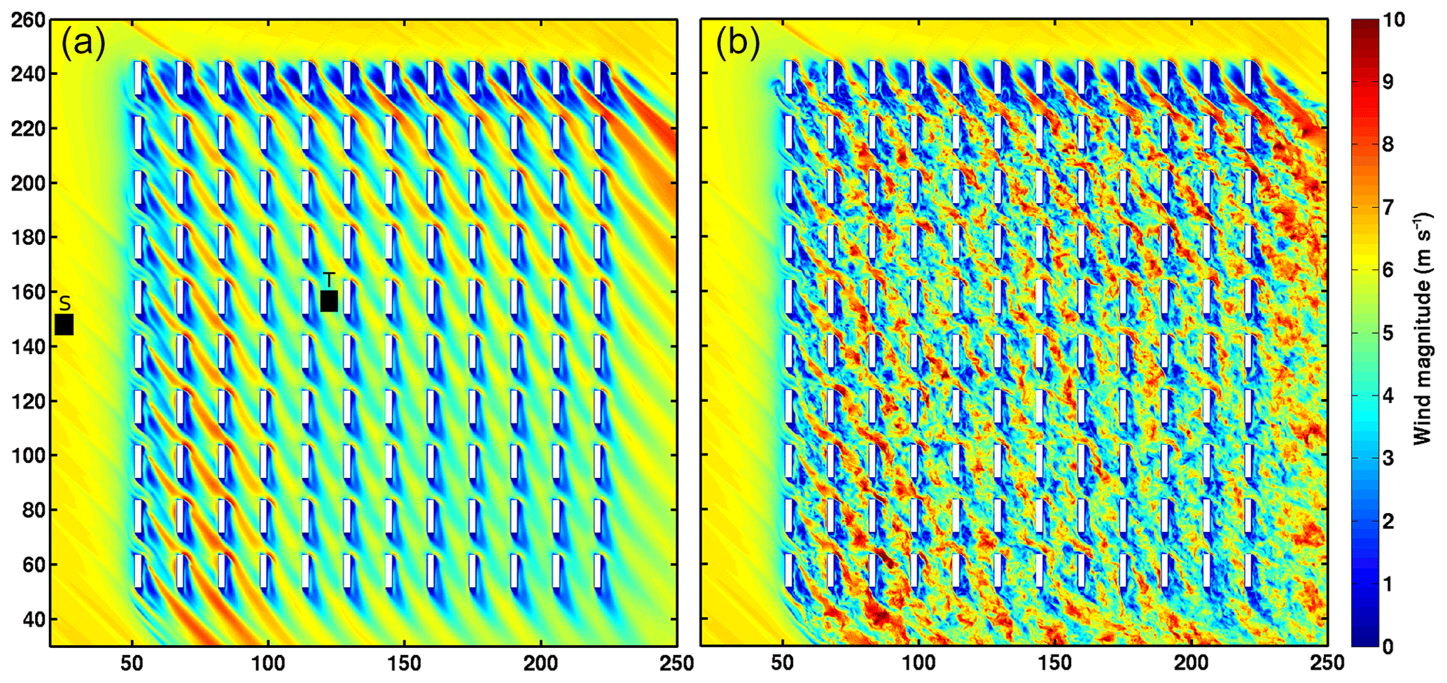
Figure 18Wind at the horizontal cut at z=1.6 m: (a) time-averaged on 200 s; (b) instantaneous at t=200 s. The black squares indicate the location of the T and S towers (MNH–IBM results).
Figure 18a (b) illustrates the time-averaged horizontal wind field ( at t=200 s) at the 1.6 m altitude. These figures highlight the fact that the incoming flow is not turbulent in the simulation. This assumed gap constitutes a perspective (Camelli et al., 2005) not directly linked to IBM. It also allows us to introduce here some comments on the turbulence state. The atmospheric turbulence is dependent on the roughness length (z0 considered constant due to the homogeneous and flat desert over a few miles upstream). The first container rows are the scene of the boundary layer transition and act as a region of strong roughness change. The turbulence observed in the urban-like canopy has two origins: the incoming turbulence and that induced by the container presence. The contribution of both turbulence types varies as a function of the altitude and distance to the first row.
Yee and Biltoft (2004)Yee and Biltoft (2004)Yee and Biltoft (2004)Table 2Kinetic energy, turbulent kinetic energy and friction velocity obtained by the experimental (Yee and Biltoft, 2004) and numerical (MNH–IBM) investigations at three altitudes of the tower T.
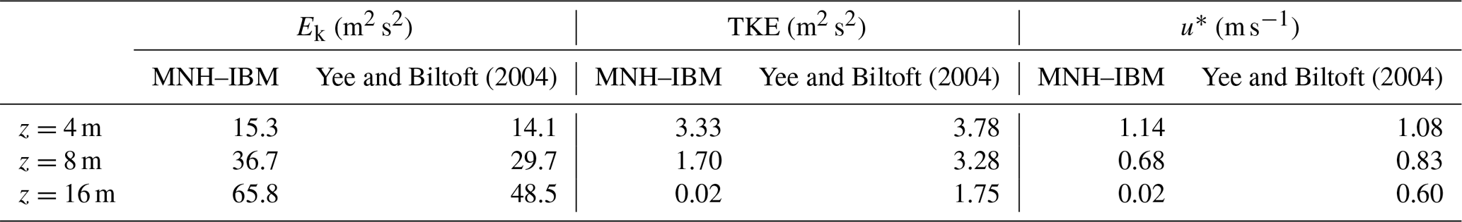
The mean kinetic energy , friction velocity and turbulent kinetic energy are estimated at the T tower and indicated in Table 2. All the variables are in good agreement with the experiment at z=4 m (about 2 times the container height). The friction velocity at z(T)=4 m is at least 2 times larger than m s−1 observed at the S tower feet. That increase is the signature of the turbulence developed by the urban-like canopy. Looking at the results at z(T)=8 m and z(T)=16 m, the higher the altitude, the more discrepancies appear between the experimental and numerical results. The experimental measurement of the friction velocity at z=16 m is close to the upstream value.
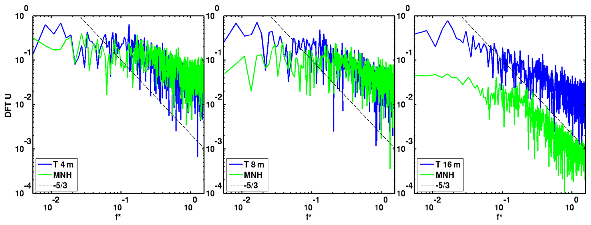
Figure 19Spectrum of the measured (blue line) and modeled (green line) u wind component at the T tower at m. f∗ is dimensionless as a Strouhal number using (z=2.5 m), and z=2.5 m is the container length.
The discrete Fourier transform of the u temporal evolution (Fig. 19) at m shows the coherence between the energetic cascade of the experimental investigations and that of the numerical ones. At z(T)=16 m, MNH–IBM underestimates the unsteady part of the solution for all wave numbers. The same behavior is observed on v and w (not shown here).
The MNH–IBM results are consistent with the experimental observations below z(T)≲10 m. This modeling induces the turbulence to be mostly due to the container wakes upstream of the T tower and not to the incoming turbulence (not modeled in the simulation). The influence of the atmospheric turbulence grows with altitude and MNH–IBM diverges with the experiment. This divergence for z(T)≳10 m leads us to think that the thickness of the container has an influence about 4–5 times the height of the urban-like canopy.
This study details the first implementation of an immersed boundary method (IBM) in the atmospheric Meso-NH (MNH) model currently based on mathematical formulations written for structured grids. The MNH–IBM aim is to explicitly model the fluid–solid interaction in the surface boundary layer developed over grounds presenting complex topographies such as cities or industrial sites.
A level-set function (Sussman et al., 1994) characterizes the geometric properties of the fluid–solid interface. Two original approaches of the ghost-cell (Tseng and Ferziger, 2003) and cut-cell techniques (Udaykumar and Shyy, 1995) are implemented to correct the MNH numerical schemes. A newly proposed GCT recovers the fluid information in several image points by presenting a distance to the interface independent of the ghost's distance. The CCT consists of a new finite-volume approach of flux balance near the immersed interface. The GCT is applied to the numerical schemes based on explicit time integration and the CCT is employed in the implicit resolution of the Poisson equation, satisfying the incompressibility hypothesis. The adaptation and use of iterative procedures solves the pressure problem without any modification to the inverted matrix. The turbulence problem is closed at the fluid–solid interface by a pragmatic LES–RANS formulation based on the subgrid turbulent kinetic energy and the length of the smallest energetic eddies.
The pressure solver, adapted to the IBM and isolated from the rest of MNH, is used to model potential flows around several obstacles. Compared to analytical and theoretical solutions, the numerical results demonstrate the ability of the IBM adaptation to ensure that the momentum is preserved and the continuity equation is respected. Non-dissipative flows are simulated to test the IBM forcing of the wind advection scheme (the impact of interpolations collected in Franke (1982), classical and novel GCT comparison, and numerical diffusion near the interface). These tests validate the proposed GCT “three images and ghost points” using an inverse distance-weighting (trilinear) interpolation near (far from) the interface. The modeling of the advection term near the fluid–solid interface is ensured by a second-order centered scheme associated with an artificial viscosity. The artificial viscosity is calibrated after comparisons with a third-order WENO scheme. With these numerical choices, MNH–IBM demonstrates its ability to model wake instabilities past a circular cylinder placed in a viscous fluid. Then, large-eddy simulations of turbulent flows around bodies with sharp edges and corners are executed (i.e., a cube placed in a channel as in Martinuzzi and Tropea, 1993, and a near-neutral atmospheric application over an array of containers as in Biltoft, 2001). These two LESs validate the proposed immersed wall model, switching the characteristic space scale defining the turbulent Reynolds number between one obtained by either a viscous length scale (the cube case) or a roughness length (the container case).
Future work. This study constitutes a first robust step towards a better understanding of the interactions between “weather and cities” and better predictions of such interactions. The idealized character of the physical cases approached here offers some insights. One improvement would consist of a generalization of the IBM writing to terrain-following coordinates (Gal-Chen and Somerville, 1975), allowing for the simulation of high-curvature bodies in the presence of non-flat ground. In the run-up of the resolution of multiscale problems, consistency with grid nesting (Stein et al., 2000) would be pertinent as would coupling to a drag model (Aumond et al., 2013). In the current paper, “simple” bodies are investigated; the modeling of real houses and buildings with arbitrary shapes in close proximity to each other is ongoing with work dedicated to a brief and intense pollutant episode due to a factory explosion in 2001 over Toulouse, assuming a dry neutral case with nonreactive gas dispersion. Such hypotheses involve a broad range of physical phenomena requiring numerical compliance with IBM, including chemical reactions, phase changes and radiative effects. Such compliance would allow for access to a large variety of atmospheric situations.
The immersed boundary method has been implemented in the 5.2 version of the Meso-NH code. This reference version is under the CeCILL-C license agreement and freely available at http://mesonh.aero.obs-mip.fr/mesonh52 (last access: 13 May 2019).
The source files dedicated to IBM and the input files for the simulations in Sects. 4 and 5 can be downloaded from the CERFACS web page: https://cerfacs.fr/MNHIBM/Auguste-GMD-2019 (Auguste, 2019). A Supplement to this article contains the tar ball (1Mo) of these files. The immersed boundary method will be integrated in a future Meso-NH version.
Array of vortices. A Poisson equation solution is investigated (Fig. A1a) by imposing in the RHS of Eq. (5) the divergence , where . The error norms (, where Pn is the numerical pressure and Pt the theoretical one) are estimated in the presence (or not) of an immersed cylindrical body (Fig. A1). The space second order of the pressure solver is recovered without IBM. The order decreases with IBM and stays consistent regarding the slopes. Note that an immersed square or sphere gives similar results.
Agnesi hill. The irrotational solution around two 2-D bell-shaped interfaces is investigated with IBM and the boundary-fitted method (BFM; terrain-following coordinates). The topography is characterized by a height ha and a shape (ka=4, bell 1; ka=8, bell 2). The bell slope is arbitrarily and respectively described here as gentle or steep. Figure A2 shows the pressure contours obtained with IBM (left) and BFM (right) for a gentle (top) and a steep (bottom) shape. The minimal pressure value is localized at the top of each bell and goes to zero far from this location. The reference BFM and IBM simulations with the fine resolution (N=160 nodes per ha, red) show a good agreement for each hill. The blue (green) corresponds to a coarser mesh employing N∕3 (N∕9) nodes per ha. Weak differences appear between the N and N∕3 meshes for both IBM and BFM, revealing a good space convergence (Fig. A2a–b). Numerical errors are visible with IBM near the interface, but the Venturi effect is well modeled. Differences become more significant with the N∕9 mesh, especially with the BFM BELL2 presenting the highest curvature value (Fig. A2d). IBM appears less accurate than BFM when the ground presents low curvature in regard to the space resolution. Otherwise, IBM seems more pertinent than BFM to model high interfaces such as sharp edges or corners. The minimum pressure that could reach −∞ is smoothed by IBM and allows the pressure solver not to diverge. Note that Lundquist et al. (2010, 2012) used a compressible WRF model and observed similar behaviors.
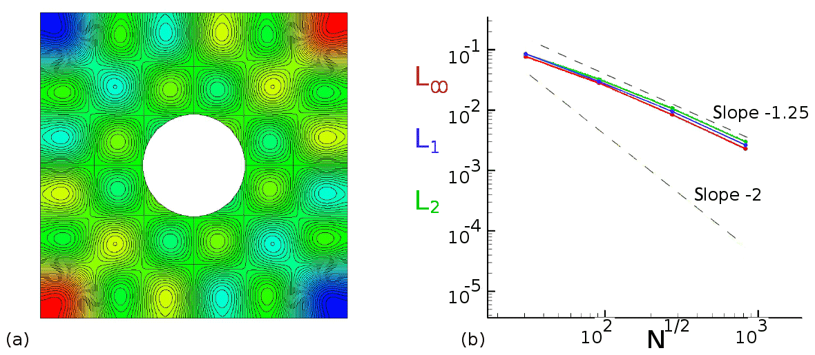
Figure A1Array of vortices around a cylinder: (a) illustration; (b) L∞, L1 and L2 norm functions of the space resolution.
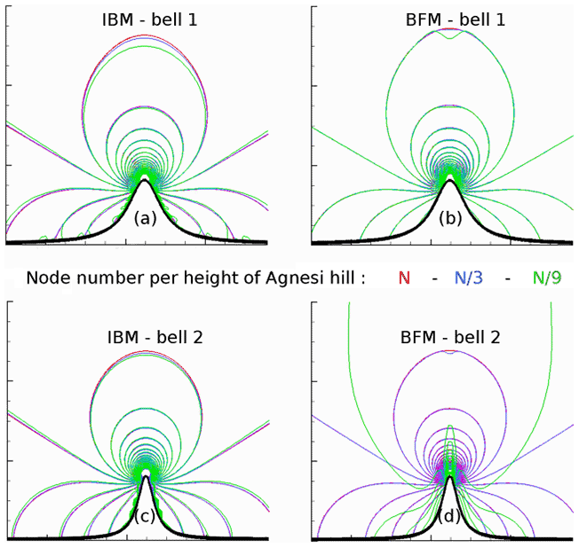
Figure A2Potential flow function of the space resolution (color code) plotting the pressure contours around two bells (a, b: BELL1, gentle slope; c, d: BELL2, steep slope) and obtained with IBM (a, c) and the boundary-fitted method (b, d).
For most atmospheric applications, the region size for which the fluid molecular viscosity νf influences the dynamic is sufficiently small to be considered negligible (Sect. 2.3). Solving the Euler equations, the impact of the numerical diffusion could be significant, especially near the fluid–solid interface. The adopted strategy with IBM is to model the advection term with a low-order scheme near the interface (Sect. 3). The order decrease in IBM is not essential but allows us to limit the number of ghosts in the solid region, thereby limiting the communications during a parallel computation. Indeed, the chosen implementation implies that the associated images and ghost points have to be localized in the integration volume of each processor. The WEN3 third-order weighted essentially non-oscillatory and CEN2 second-order centered schemes are available in MNH. Far from the interface a CEN4 fourth-order centered scheme is employed. Table B1 summarizes the advection scheme nomenclature.
The vorticity equation for a 2-D inviscid flow reveals no production in time. The numerical vorticity production at the immersed surface of a cylindrical body is studied here by initializing the simulation with the potential solution. To fit the potential solution, a nontrivial condition is employed on the tangent velocity . Expecting a numerical vorticity sufficiently controlled to avoid the flow separation, the effect of the artificial diffusion injected with CEN2 is compared to the WEN3 intrinsically diffusive behavior. Furthermore, this study had estimated the 3-D interpolation impact (not detailed here).
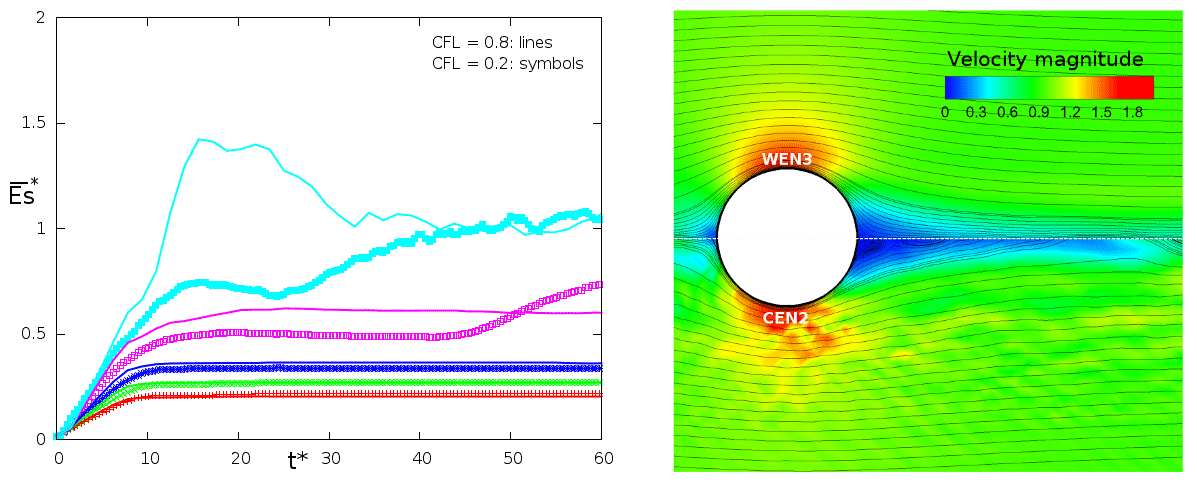
Figure B1Solving the Euler equations: (a) vorticity production influenced by the Courant number (CFL = 0.8, line; CFL = 0.2, symbol) and by the νart artificial viscosity (red, green, blue, purple and cyan, respectively; ) using an advection CEN2 second-order centered scheme near the interface; (b) velocity magnitude field obtained with a WEN3 third-order weighted essentially non-oscillatory scheme (top) and (bottom). CEN4 is the advection scheme used far from the interface. The mesh is the coarser one (MESH1).
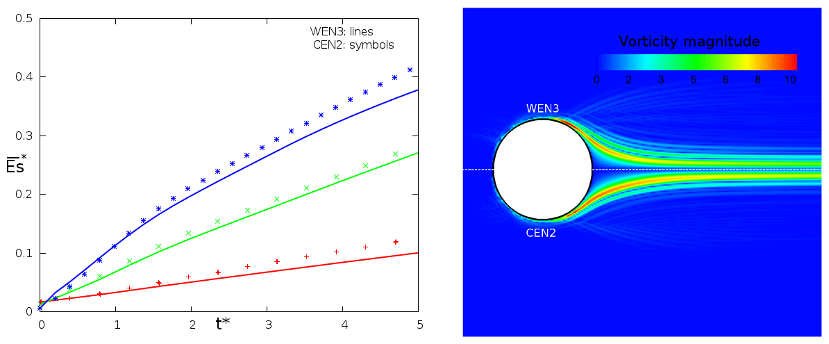
Figure B2Solving the Euler equations: (a) influence of the space resolution (red: MESH1; green: MESH2; blue: MESH3) on the vorticity production when the near-interface advection is modeled by WEN3 (line) and (symbol); (b) vorticity magnitude field obtained by WEN3 (top) and (bottom).
Figure B1a plots the evolution in time of the enstrophy depending on the Δt time step and νart using CEN2 near the interface (with U∞ the velocity of the incoming flow and 𝒱f the integration volume in the fluid region). The enstrophy increases in time and reaches a mean value when the produced vorticity near the interface is evacuated from the numerical domain and in the body wake. Except for the simulations with low artificial diffusion (symbols and curves in cyan and purple), the vorticity production is weakly dependent on the physical time and CFL Courant number (symbols and curves in red, green and blue). It induces νart proportional to . A reference value of the artificial viscosity is also defined as .
Figure B1b illustrates the vorticity field in the vicinity of the interface between the intrinsically diffusive WEN3 and CEN2+νart with . The streamlines are maintained without detachment near the interface with WEN3. Otherwise, the CEN2 solution with low artificial diffusion presents numerical instabilities and vortex shedding.
Table B1Summary of the mean wind advection scheme used (WENO: weighted essentially non-oscillatory).
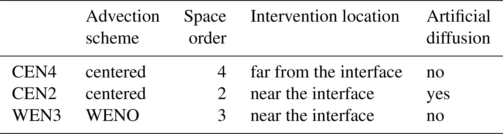
Figure B2a plots the enstrophy evolution for three meshes (color code) for WEN3 (lines) and CEN2+νart with (symbols). MESH1 (10 nodes per Dcyl), MESH2 (20 nodes per Dcyl) and MESH3 (40 nodes per Dcyl) are respectively the coarse, intermediate and fine mesh. The border of the numerical domain is always distant from the cylinder of more than 10Rcyl. The CEN2+ vorticity production appears fairly close to the WEN3 one for the three space resolutions. Figure B2b corroborates the last comment, presenting the vorticity contours dimensionless by . A suitable νart combined with the CEN2 choice is also in the range of the too-diffusive WEN3 results and the growth of numerical instabilities. CEN2+ is retained as the advection scheme of the mean wind near an immersed interface.
The supplement related to this article is available online at: https://doi.org/10.5194/gmd-12-2607-2019-supplement.
All authors contributed to the development of the source code. The execution and the exploitation of the presented simulations were conducted by FA and GR. All authors contributed to the writing and editing of the paper.
The authors declare that they have no conflict of interest.
We thank the following for stimulating and fruitful discussions: Jacques Magnaudet (Institut de Mécanique des Fluides, IMFT, Toulouse), Yannick Hallez (Laboratoire de Génie Chimique de Toulouse, LGC, Toulouse), Jean-Lou Pierson (Institut Francais du Pétrole Energies Nouvelles, IFPEN, Lyon), Jean-Luc Redelsperger (Laboratoire de Physique des Océans, IFREMER, Brest), Jean-Pierre Pinty and Juan Escobar (Laboratoire d'Aérologie, LA, Toulouse), Odile Thouron, Thibaut Lunet, Luc Giraud, Isabelle d'Ast and Gerard Dejean (Centre Européen de Recherche et Formation Avancée en Calcul Scientifique, CERFACS, Toulouse). The simulations were performed on the Neptune/Nemo-CERFACS supercomputers on the Occigen-CINES Bull cluster (c2016017724 and a0010110079 GENCI projects).
Part of this work was supported by Région Midi-Pyrénées funding.
This paper was edited by Ignacio Pisso and reviewed by two anonymous referees.
Allwine, K. J., Shinn, J. H., Streit, G. E., Clawson, K. L., and Brown, M.: Overview of URBAN 2000: A multiscale field study of dispersion through an urban environment, B. Am. Meteorol. Soc., 83, 521–536, 2002. a
Angot, P., Bruneau, C. H., and Fabrie, P.: A penalization method to take into account obstacles in incompressible viscous flows, Numer. Math., 81, 497–520, 1999. a
Auguste, F.: Instabilités de sillage et de trajectoire dans un fluide visqueux, PhD thesis, University of Toulouse, Toulouse, France, 2010. a
Auguste, F.: MNH-IBM: Source code and input files, available at: https://cerfacs.fr/MNHIBM/Auguste-GMD-2019, last access: 13 May 2019. a
Aumond, P., Masson, V., Lac, C., Gauvreau, B., Dupont, S., and Berengier, M.: Including the drag effects of canopies: real case large-eddy simulation studies, Bound.-Lay. Meteorol., 146, 65–80, 2013. a, b
Batchelor, G. K.: An introduction to fluid dynamics, Cambridge university press, Cambridge, UK, 2000. a, b
Bernadet, P.: The pressure term in the anelastic model: A symmetric elliptic solver for an Arakawa C grid in generalized coordinates, Mon. Weather Rev., 123, 2474–2490, 1995. a
Biltoft, C. A.: Customer report for mock urban setting test, DPG Document Number 8-CO-160-000-052. Prepared for the Defence Threat Reduction Agency, Dugway, Utah, USA, 2001. a, b, c
Biltoft, C. A., Yee, E., and Jones, C. D.: Overview of the Mock Urban Setting Test (MUST), in: Proceedings of the Fourth Symposium on the Urban Environment, 19 May 2002, Norfolk, VA, USA, 20–24, 2002. a
Bouchon, F., Dubois, T., and James, N.: A second-order cut-cell method for the numerical simulation of 2D flows past obstacles, Comput. Fluids, 65, 80–91, 2012. a
Braza, M., Chassaing, P., and Minh, H. H.: Numerical study and physical analysis of the pressure and velocity fields in the near wake of a circular cylinder, J. Fluid Mech., 165, 79–130, 1986. a
Bredberg, J.: On the wall boundary condition for turbulence models, Chalmers University of Technology, Department of Thermo and Fluid Dynamics, Internal Report 00/4, Goteborg, Sweden, 2000. a, b
Brennen, C. E.: A Review of Added Mass and Fluid Inertial Forces, Naval Civil Engineering Laboratory, Port Hueneme, CA, USA, CR 82.010, 1982. a
Breuer, M., Lakehal, D., and Rodi, W.: Flow around a surface mounted cubical obstacle: comparison of LES and RANS-results, Computation of Three-Dimensional Complex Flows, Vieweg+ Teubner Verlag, 22–30, https://doi.org/10.1007/978-3-322-89838-8, 1996. a
Businger, J. A., Wyngaard, J. C., Izumi, Y., and Bradley, E.: Flux profile relationship in the atmospheric surface layer, J. Atmos. Sci., 28, 181–189, 1971. a
Cai, S.-G., Ouahsine, A., Favier, J., and Hoarau, Y.: Moving immersed boundary method, Int. J. Numer. Meth. Fl., 85, 288–323, 2017. a, b
Camelli, F., Lohner, R., and Hanna, S.: VLES study of MUST experiment, 43rd AIAA Aerospace Sciences Meeting and Exhibit, 10–13 January 2005, Reno, Nevada, USA, 2005. a
Capizzano, F.: Turbulent wall model for immersed boundary methods, AIAA J., 49, 2367–2381, 2011. a
Carpenter, K. M.: Note on the paper “Radiation conditions for lateral boundaries of limited area numerical models”, Q. J. Roy. Meteor. Soc., 110, 717–719M, 1982. a
Castro, I. P. and Robins, A. G.: The flow around a surface-mounted cube in uniform and turbulent streams, J. Fluid Mech., 79, 307–335, 1977. a
Clarke, D. K., Hassan, H. A., and Salas, M. D.: Euler calculations for multielement airfoils using Cartesian grids, AIAA J., 24, 353–358, 1986. a
Clawson, K. L., Carter, R. G., Lacroix, D. J., Biltoft, C. A., Hukari, N. F., Johnson, R. C., Rich, J. D., Beard, S. A., and Strong, T.: Joint Urban 2003 (JU03) SF6 atmospheric tracer field tests, US Department of Commerce, National Oceanic and Atmospheric Administration, Office of Oceanic and Atmospheric Research, Air Resources Laboratory, Idaho, USA, 2005. a
Colella, P. and Woodward, P. R.: Application of the Piecewise Parabolic Method to meteorological modeling, J. Comput. Phys., 54, 174–201, 1984. a
Coutanceau, M. and Bouard, R.: Experimental determination of the main features of the viscous flow in the wake of a circular cylinder in uniform translation. Part I – Steady flow, J. Fluid Mech., 79, 231–256, 1977. a
Craft, T., Gant, S., Gerasimov, A., Iacovides, H., and Launder, B.: Wall Functions Strategies for Use in Turbulent Flow CFD, Heat Transfer, 1, 3–14, 2002. a, b
Cuxart, J., Bougeault, P., and Redelsperger, J.-L.: A turbulence scheme allowing for mesoscale and large-eddy simulations, Q. J. Roy. Meteor. Soc., 126, 1–30, 2000. a
Dejoan, A., Santiago, J.-L., Martilli, A., Martin, F., and Pinelli, A.: Comparison between large-eddy simulation and Reynolds-averaged Navier–Stokes computations for the MUST field experiment. Part II: effects of incident wind angle deviation on the mean flow and plume dispersion, Bound.-Lay. Meteorol., 135, 133–150, 2010. a
Depardon, S., Lasserre, J. J., Brizzi, L. E., and Borée, J.: Instantaneous skin-friction pattern analysis using automated critical point detection on near-wall PIV data, Meas. Sci. Technol., 17, 1659–1669, 2006. a
Donnelly, R. P., Lyons, T. J., and Flassak, T.: Evaluation of results of a numerical simulation of dispersion in an idealised urban area for emergency response modelling, J. Atmos. Environ., 43, 4416–4423, 2009. a
Durran, D. R.: Improving the anelastic approximation, J. Atmos. Sci., 46, 1452–1461, 1989. a
Farhadi, M. and Rahnama, M.: Large eddy simulation of separated flow over a wall-mounted cube, Sci. Iran., 13, 124–133, 2006. a, b
Frank, W.: Numerical Simulation And Verification Of The Flow Around A Surface Mounted Cubic Body Placed In A Fully Developed Turbulent Channel Flow, WIT Trans. Model. Sim., 22, 213–222, 1999. a, b
Franke, R.: Scattered data interpolation, tests of some methods, Math. Comput., 38, 181–200, 1982. a, b
Gal-Chen, T. and Somerville, R. C.: On the use of a coordinate transformation of the Navier-Stokes equations, J. Comput. Phys., 17, 209–228, 1975. a, b
Gautier, R., Biau, D., and Lamballais, E.: A reference solution of the flow over a circular cylinder at Re=40, Comput. Fluids, 75, 103–111, 2013. a, b
Goldstein, D., Handler, R., and Sirovich, L.: Modeling a no-slip flow boundary with an external force field, J. Comput. Phys., 105, 354–366, 1993. a
Hanna, S. R., Hansen, O. R., and Dharmavaram, S.: FLACS CFD air quality model performance evaluation with Kit Fox, MUST, Prairie Grass, and EMU observations, J. Atmos. Env., 38, 4675–4687, 2004. a
Hidalgo, J., Pigeon, G., and Masson, V.: Urban-breeze circulation during the CAPITOUL experiment: observational data analysis approach, Meteorol. Atmos. Phys., 102, 223–241, 2008. a
Hunt, J. C., Wray, A. A., and Moin, P.: Eddies, streams and convergence zones in turbulent flows, Proceedings of the 1988 Summer Program. NASA Centre for Turbulence Research, Stanford, USA, 193–208, 1988. a, b
Hussein, H. J. A. and Martinuzzi, R. J.: Energy balance for turbulent flow around a surface mounted cube placed in a channel, Phys. Fluids, 8, 764–780, 1996. a, b, c, d, e, f
Jiang, G.-S. and Shu, C.-W.: Efficient Implementation of Weighted ENO Schemes, J. Comput. Phys., 126, 202–228, 1996. a
Kalitzin, G., Medic, G., Iaccarino, G., and Durbin, P.: Near-wall behavior of RANS turbulence models and implications for wall functions, J. Comput. Phys., 204, 265–291, 2005. a
Kanda, M., Kanega, M., Kawai, T., Moriwaki, R., and Sugawara, H.: Roughness lengths for momentum and heat derived from outdoor urban scale models, J. Appl. Meteorol. Clim., 46, 1067–1079, 2007. a
Kempe, T. and Fröhlich, J.: An improved immersed boundary method with direct forcing for the simulation of particle laden flows, J. Comput. Phys., 231, 3663–3684, 2012. a
Kim, J., Kim, D., and Choi, H.: An immersed-boundary finite-volume method for simulations of flow in complex geometries, J. Comput. Phys., 171, 132–150, 2001. a
König, M.: Large-eddy simulation modelling for urban Scale, PhD thesis, University of Leipzig, Leipzig, Germany, 2014. a
Krajnovic, S. and Davidson, L.: Development of large-eddy simulation for vehicle aerodynamics, International Mechanical Engineering Congress and Exposition, Proceedings of IMECE2002, ASME, 17–22 November 2002, New Orleans, Louisiana, USA, 2002. a, b
Lac, C., Chaboureau, J.-P., Masson, V., Pinty, J.-P., Tulet, P., Escobar, J., Leriche, M., Barthe, C., Aouizerats, B., Augros, C., Aumond, P., Auguste, F., Bechtold, P., Berthet, S., Bielli, S., Bosseur, F., Caumont, O., Cohard, J.-M., Colin, J., Couvreux, F., Cuxart, J., Delautier, G., Dauhut, T., Ducrocq, V., Filippi, J.-B., Gazen, D., Geoffroy, O., Gheusi, F., Honnert, R., Lafore, J.-P., Lebeaupin Brossier, C., Libois, Q., Lunet, T., Mari, C., Maric, T., Mascart, P., Mogé, M., Molinié, G., Nuissier, O., Pantillon, F., Peyrillé, P., Pergaud, J., Perraud, E., Pianezze, J., Redelsperger, J.-L., Ricard, D., Richard, E., Riette, S., Rodier, Q., Schoetter, R., Seyfried, L., Stein, J., Suhre, K., Taufour, M., Thouron, O., Turner, S., Verrelle, A., Vié, B., Visentin, F., Vionnet, V., and Wautelet, P.: Overview of the Meso-NH model version 5.4 and its applications, Geosci. Model Dev., 11, 1929–1969, https://doi.org/10.5194/gmd-11-1929-2018, 2018. a
Lafore, J. P., Stein, J., Asencio, N., Bougeault, P., Ducrocq, V., Duron, J., Fischer, C., Héreil, P., Mascart, P., Masson, V., Pinty, J. P., Redelsperger, J. L., Richard, E., and Vilà-Guerau de Arellano, J.: The Meso-NH Atmospheric Simulation System. Part I: adiabatic formulation and control simulations, Ann. Geophys., 16, 90–109, https://doi.org/10.1007/s00585-997-0090-6, 1998. a
Lamb, H.: Hydrodynamics, Cambridge university press, Cambridge, USA, 1932. a, b
Leveque, R. J. and Li, Z.: The immersed interface method for elliptic equations with discontinuous coefficients and singular sources, SIAM J. Numer. Anal., 31, 1019–1044, 1994. a
Lin, S. and Rood, R. B.: Multidimensional Flux-Form Semi-Lagrangian Transport Schemes, Mon. Weather Rev., 124, 2046–2070, 1996. a
Linnick, M. N. and Fasel, H. F.: A high-order immersed interface method for simulating unsteady incompressible flows on irregular domains, J. Comput. Phys., 204, 157–192, 2005. a
Lipps, F. and Hemler, R. S.: A scale analysis of deep moist convection and some related numerical calculations, J. Atmos. Sci., 39, 2192–2210, 1982. a
Liu, Y., Chen, F., Warner, T., and Basara, J.: Verification of a mesoscale data-assimilation and forecasting system for the Oklahoma City area during the Joint Urban 2003 field project, J. Appl. Meteorol. Clim., 45, 912–929, 2006. a
Lund, T. S.: Generation of Turbulent Inflow Data for Spatially-Developing Boundary Layer Simulations, J. Comput. Phys., 140, 233-–258, 1998. a
Lundquist, K. A., Chow, F. K., and Lundquist, J. K.: An immersed boundary method for the Weather Research and Forecasting model, Mon. Weather Rev., 138, 796–817, 2010. a, b
Lundquist, K. A., Chow, F. K., and Lundquist, J. K.: An immersed boundary method enabling large-eddy simulations of flow over complex terrain in the WRF model, Mon. Weather Rev., 140, 3936–3955, 2012. a, b
Lunet, T., Lac, C., Auguste, F., Visentin, F., Masson, V., and Escobar, J.: Combination of WENO and explicit Runge-Kutta methods for wind transport in Meso-NH model, Mon. Weather Rev., 145, 3817–3838, 2017. a
Martinuzzi, R. and Tropea, C.: The flow around surface-mounted, prismatic obstacles placed in a fully developed channel flow, J. Fluid. Eng.-T. ASME, 115, 85–85, 1993. a, b, c, d, e, f, g, h
Masson, V., Gomes, L., Pigeon, G., Liousse, C., Pont, V., Lagouarde, J.-P., Voogt, J., Salmond, J., Oke, T., Hidalgo, J., Legain, D., Garrouste, O., Lac, C., Connan, O., Briottet, X., Lachérade, S., and Tulet, P.: The canopy and aerosol particles interactions in Toulouse urban layer (CAPITOUL) experiment, Meteorol. Atmos. Phys., 102, 135–157, 2008. a
Masson, V., Le Moigne, P., Martin, E., Faroux, S., Alias, A., Alkama, R., Belamari, S., Barbu, A., Boone, A., Bouyssel, F., Brousseau, P., Brun, E., Calvet, J.-C., Carrer, D., Decharme, B., Delire, C., Donier, S., Essaouini, K., Gibelin, A.-L., Giordani, H., Habets, F., Jidane, M., Kerdraon, G., Kourzeneva, E., Lafaysse, M., Lafont, S., Lebeaupin Brossier, C., Lemonsu, A., Mahfouf, J.-F., Marguinaud, P., Mokhtari, M., Morin, S., Pigeon, G., Salgado, R., Seity, Y., Taillefer, F., Tanguy, G., Tulet, P., Vincendon, B., Vionnet, V., and Voldoire, A.: The SURFEXv7.2 land and ocean surface platform for coupled or offline simulation of earth surface variables and fluxes, Geosci. Model Dev., 6, 929–960, https://doi.org/10.5194/gmd-6-929-2013, 2013. a, b
Mayor S., Spalart P., and Tripoli, G. J.: Application of a Perturbation Recycling Method in the Large-Eddy Simulation of a Mesoscale Convective Internal Boundary Layer, J. Atmos. Sci., 59, 2385–2395, 2002. a
Milliez, M. and Carissimo, B.: Numerical simulations of pollutant dispersion in an idealized urban area, for different meteorological conditions, Bound.-Lay. Meteorol., 122, 321–342, 2007. a, b
Milne-Thomson, L. M.: Theoretical hydrodynamics, Dover Books on Physics Series, Dover Publications, 1968. a
Mittal, R. and Iaccarino, G.: Immersed Boundary Methods, Annu. Rev. Fluid Mech., 37, 239–261, 2005. a, b
Mohd-Yusof, J.: Combined immersed-Boundary/B-Spline methods for simulations of flow in complex geometries, CTR Annual Research Briefs, NASA Research Center/Stanford University, Center for Turbulence Research, Stanford, CA, USA, 1997. a
Monin, A. S. and Obukhov, A. M. F.: Basic laws of turbulent mixing in the surface layer of the atmosphere, Contrib. Geophys. Inst. Acad. Sci. USSR, 151, 163–187, 1954. a
Moriwaki, R. and Kanda, M.: Seasonal and diurnal fluxes of radiation, heat, water vapor, and carbon dioxide over a suburban area, J. Appl. Meteorol., 43, 1700–1710, 2004. a
Park, J., Kwon, K., and Choi, H.: Numerical solutions of flow past a circular cylinder at Reynolds numbers up to 160, KSME Int. J., 12, 1200–1205, 1998. a
Peskin, C. S.: Flow patterns around heart valves: a numerical method, J. Comput. Phys., 10, 252–271, 1972. a
Pierson, J.-L.: Traversée d'une interface entre deux fluides par une sphère, PhD thesis, University of Toulouse, Toulouse, France, 2015. a
Piomelli, U. and Balaras, E.: Wall-layer models for large-eddy simulations, Annu. Rev. Fluid Mech., 34, 349–374, 2002. a
Prandtl, L.: Bericht über Untersuchungen zur ausgebildeten Turbulenz, Z. Angew. Math, Meth., 5, 136–139, 1925. a
Redelsperger, J.-L. and Sommeria, G.: Methode de representation de la turbulence inferieure a la maille pour un modele tri-dimensionnel de convection nuageuse, Bound.-Lay. Meteorol., 21, 509–530, 1981. a
Redelsperger, J.-L., Mahe, F., and Carlotti, P.: A simple and general subgrid model suitable both surface layer and free-stream turbulence, Bound.-Lay. Meteorol., 101, 375–408, 2001. a
Rodi, W., Ferziger, J. H., Breuer, M., and Pourquie, M.: Status of large eddy simulation: results of a workshop, J. Fluid. Eng.-T. ASME, 119, 248–262, 1997. a, b
Schumann, U. and Sweet, R.: Fast Fourier Transforms for direct solution of Poisson's equations with staggered boundary conditions, J. Comput. Phys., 75, 123–137, 1988. a, b
Shah, K. B. and Ferziger, J. H.: A fluid mechanicians view of wind engineering: Large eddy simulation of flow past a cubic obstacle, J. Wind Eng. Ind. Aerod., 67, 211–224, 1997. a, b, c
Shu, C.-W. and Osher, S.: Efficient implementation of essentially non-oscillatory shock capturing schemes, J. Comput. Phys., 83, 32–78, 1989. a
Skamarock, W. C., Smolarkiewicz, P. K., and Klemp, J. B.: Preconditioned conjugate-residual solvers for Helmhotz equations in nonhydrostatic models, Mon. Weather Rev., 125, 587–599, 1997. a
Stålberg, E., Brüger, A., Lötstedt, P., Johansson, A. V., and Henningson, D. S.: High order accurate solution of flow past a circular cylinder, J. Sci. Comput., 27, 431–441, 2006. a
Stein, J., Richard, E., Lafore, J.-P., Pinty, J.-P., Asencio, N., and Cosma, S.: High-resolution non-hydrostatic simulations of flash-flood episodes with grid-nesting and ice-phase parametrization, Meteorol. Atmos. Phys., 72, 101–110, 2000. a
Straka, J. M., Wilhelmson, R. B., Wicker, L. J., Anderson, J. R., and Droegemeier, K. K.: Numerical solutions of a non-linear density current: A benchmark solution and comparisons, Int. J. Numer. Meth. Fl., 17, 1–22, 1993. a
Sussman, M., Smereka, P., and Osher, S.: A level set approach for computing solutions to incompressible two-phase flow, J. Comput. Phys., 114, 146–159, 1994. a, b, c
Taira, K. and Colonius, T.: The immersed boundary method: a projection approach, J. Comput. Phys., 225, 2118–2137, 2007. a
Taneda, S.: Experimental investigation of the wake behind a sphere at low Reynolds numbers, J. Phys. Soc. Jpn., 11, 1104–1108, 1956. a, b, c
Tseng, Y. H. and Ferziger, J. H.: A ghost-cell immersed boundary method for flow in complex geometry, J. Comput. Phys., 192, 593–623, 2003. a, b, c
Udaykumar, H. S. and Shyy, W.: A grid-supported marker particle scheme for interface tracking, Numer. Heat Transfer, 27, 127–153, 1995. a
von Kármán, T.: Mechanische Änlichkeit und Turbulenz, Proceedings of the Third International Congress of Applied Mechanics, 24–29 August 1930, Stockholm, Sweden, Part I, 1930. a, b
Wang, K., Li, Y., Li, Y., and Yuan, M.: The stone forest as a small-scale field model for urban climate studies, 9th International Conference on Urban Climate (ICUC9), 20–24 July 2015, Toulouse, France, 2015. a
Williamson, C. H. K.: Oblique and parallel modes of vortex shedding in the wake of a circular cylinder at low Reynolds numbers, J. Fluid Mech., 206, 579–627, 1989. a, b
Yang, G., Causon, D. M., Ingram, D. M., Saunders, R., and Batten, P.: A Cartesian cut cell method for compressible flows part A: Static body problems, Aeronaut. J., 101, 47–56, 1997. a
Yang, X. I. and Meneveau, C.: Recycling inflow method for simulations of spatially evolving turbulent boundary layers over rough surfaces, J. Turbul., 17, 75–93, 2016. a
Ye, T., Mittal, R., Udaykumar, H. S., and Shyy, W.: An accurate Cartesian grid method for viscous incompressible flows with complex immersed boundaries, J. Comput. Phys., 156, 209–240, 1999. a
Yee, E. and Biltoft, C. A.: Concentration fluctuation measurements in a plume dispersing through a regular array of obstacles, Bound.-Lay. Meteorol., 111, 363–415, 2004. a, b, c, d, e, f, g, h
Young, D. M. and Jea, K. C.: Generalized conjugate-gradient acceleration of nonsymmetrizable iterative methods, Linear Algebra Appl., 34, 159–194, 1980. a
Meso-NH scientific documentation: http://mesonh.aero.obs-mip.fr/mesonh52/BooksAndGuides (last access: 13 May 2019).
- Abstract
- Introduction
- The Meso-NH code at a glance
- The IBM forcing in the Meso-NH code
- Flows around a circular cylinder
- Turbulent flows around parallelepiped(s)
- Conclusions and perspectives
- Code availability
- Appendix A: Space convergence of the pressure solver
- Appendix B: Inviscid flow around a circular cylinder
- Author contributions
- Competing interests
- Acknowledgements
- Financial support
- Review statement
- References
- Supplement