the Creative Commons Attribution 4.0 License.
the Creative Commons Attribution 4.0 License.
 | 08 Jul 2019
Regionally refined test bed in E3SM atmosphere model version 1 (EAMv1) and applications for high-resolution modeling
Stephen A. Klein
Shaocheng Xie
Wuyin Lin
Jean-Christophe Golaz
Erika L. Roesler
Mark A. Taylor
Philip J. Rasch
David C. Bader
Larry K. Berg
Peter Caldwell
Scott E. Giangrande
Richard B. Neale
Yun Qian
Laura D. Riihimaki
Charles S. Zender
Yuying Zhang
Xue Zheng
Climate simulations with more accurate process-level representation at finer resolutions (<100 km) are a pressing need in order to provide more detailed actionable information to policy makers regarding extreme events in a changing climate. Computational limitation is a major obstacle for building and running high-resolution (HR, here 0.25∘ average grid spacing at the Equator) models (HRMs). A more affordable path to HRMs is to use a global regionally refined model (RRM), which only simulates a portion of the globe at HR while the remaining is at low resolution (LR, 1∘). In this study, we compare the Energy Exascale Earth System Model (E3SM) atmosphere model version 1 (EAMv1) RRM with the HR mesh over the contiguous United States (CONUS) to its corresponding globally uniform LR and HR configurations as well as to observations and reanalysis data. The RRM has a significantly reduced computational cost (roughly proportional to the HR mesh size) relative to the globally uniform HRM. Over the CONUS, we evaluate the simulation of important dynamical and physical quantities as well as various precipitation measures. Differences between the RRM and HRM over the HR region are predominantly small, demonstrating that the RRM reproduces the precipitation metrics of the HRM over the CONUS. Further analysis based on RRM simulations with the LR vs. HR model parameters reveals that RRM performance is greatly influenced by the different parameter choices used in the LR and HR EAMv1. This is a result of the poor scale-aware behavior of physical parameterizations, especially for variables influencing sub-grid-scale physical processes. RRMs can serve as a useful framework to test physics schemes across a range of scales, leading to improved consistency in future E3SM versions. Applying nudging-to-observations techniques within the RRM framework also demonstrates significant advantages over a free-running configuration for use as a test bed and as such represents an efficient and more robust physics test bed capability. Our results provide additional confirmatory evidence that the RRM is an efficient and effective test bed for HRM development.
- Article
(28136 KB) - Full-text XML
- BibTeX
- EndNote


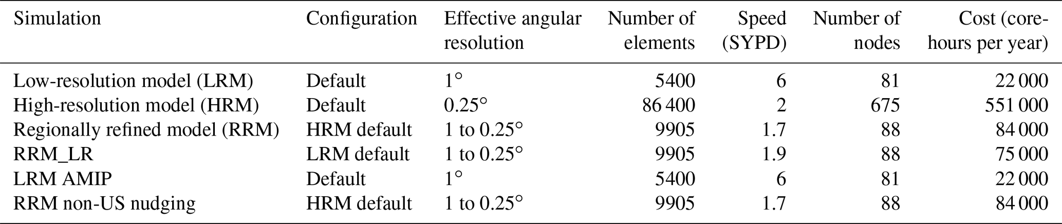
A key goal of the United States (US) Department of Energy (DOE) Energy Exascale Earth System Model (E3SM) project (formally known as the Accelerated Climate Modeling for Energy, ACME) is to develop a high-resolution (HR, 0.25∘ or finer in the horizontal) fully coupled Earth system model for climate simulation and prediction (Bader et al., 2014). Testing new physical parameterizations and tuning loosely constrained parameters within existing parameterizations are important steps of model development. However, the computational cost of running a globally uniform HR model (HRM) is high. For example, a 1-year 0.25∘ HR E3SM atmosphere model version 1 (EAMv1) simulation requires 0.6 million core hours on 675 “Knights Landing” (KNL, Intel Xeon Phi Processor 7250) nodes of the Cori supercomputer at the National Energy Research Scientific Computing Center (NERSC). A regionally refined model (RRM) capability (Ringler et al., 2008; Zarzycki and Jablonowski, 2014; Roesler et al., 2019), which only simulates a fraction of the globe at HR, is adopted by EAMv1 to reduce the computational cost of HR simulations and to examine the parameterization sensitivity to HR scales. The RRM simulation cost is usually dominated by the computational cost of the HR region, and thus the total model cost is roughly proportional to the size of the region with finer resolution, referred to as a “mesh” (typically chosen to be about 10 % of the globe, making the cost about 10 % of a uniform HRM simulation). In the ongoing E3SM phase II project, the RRM configuration is planned as a central tool to achieve the E3SMv2 science goal of understanding the relative impacts of global forcing versus regional influences of human activities on flood and drought in North America. RRM will be routinely used over North America to address DOE's goal of understanding the Earth system changes affecting US energy-sector decisions. It will be also applied as a physics test bed to improve the scale awareness of parameterizations in upcoming versions of E3SMv2 and v3 as well as an important strategy to perform a larger ensemble of HR simulations. RRM is also a vital capability for progress towards an eventual global cloud-resolving model with 3 km horizontal grid spacing targeting E3SMv4 and beyond.
The RRM approach has been established and validated with other models over many regions of interest. For instance, Zarzycki et al. (2014) showed the effectiveness of an RRM with aquaplanet experiments using the Community Atmosphere Model (CAM). Zarzycki and Jablonowski (2014, 2015) demonstrated improved skill in simulating tropical cyclones in CAM with a refined mesh over the North Atlantic. Rhoades et al. (2016) and Wu et al. (2017) depicted that the variable-resolution (VR) Community Earth System Model (CESM) was able to accurately capture the climatology and seasonality of important variables over mountain regions. Huang and Ullrich (2017) reproduced the geographic patterns of historical precipitation climatology over the western US with the VR-CESM. Gettelman et al. (2018) performed comprehensive tests of a VR dynamical core in CESM2 and showed that VR grids were feasible alternatives to conventional nesting for regional climate research. Roesler et al. (2019) found that refining the grid over the contiguous United States (CONUS) did not exert a noticeable influence on the global circulation in the EAM version 0 (EAMv0, which is almost identical to CAM5.3 except for some minor tunings and bug fixes). These earlier studies have demonstrated that RRMs can be used as an effective tool to study important climate features over regions of interest with high resolution.
Compared to EAMv0, EAMv1 (Rasch et al., 2019) includes significant changes to its physics, substantially increased vertical resolution, retuning, and bug fixes (Zhang et al., 2018). All these changes cause the model to behave very differently from EAMv0, especially in terms of regional clouds and precipitation characteristics (Xie et al., 2018). Given these substantial model changes and the critical role that RRM will play in future E3SM scientific applications, this paper documents further scientific analysis of RRM behavior with EAMv1. We contrast simulations between the RRM and the globally uniform HR EAMv1 over the RRM region, with the goal of providing more insights into the EAMv1 RRM capability to the user community. This study emphasizes hydrology-related simulation skill over North America: a key element of the E3SM Water Cycle science driver. We investigate whether RRM reproduces the same performance as HRM of these fields enabling it to be used as an effective physics test bed for understanding physical processes and improving their representations in EAMv1 and in future versions. In addition, EAMv1 physical parameterizations (and in particular the cloud parameterizations) are not inherently scale-aware and hence require retuning when increasing model horizontal or vertical resolution. Unfortunately, this leads to two different parameter settings for EAMv1 high- and low-resolution models. It is key to determine how the two different parameter settings influence RRM performance, since most earlier studies just used the established low-resolution model parameters over the RRM domain, which may not yield optimal RRM results due to scale-aware shortcomings of the existing physical schemes.
This study centers mainly on “proof-of-concept” examples. More in-depth analysis of RRM behavior will be reported in separate studies when RRM is more routinely used in E3SM phase II and by general users. In many EAMv1 application scenarios, it is expected that the RRM will be more feasible and practical than the HRM. This could include evaluation against regional measurements, uncertainty quantification studies that typically demand a large ensemble size (Qian et al., 2016, 2018), and users with limited computational resource. Findings from this study regarding the strengths and weaknesses of the EAMv1 RRM configuration should provide valuable guidance for future RRM applications in the HR E3SM development and broad community use of the E3SM RRM.
Additionally, we provide detailed information on how to utilize the RRM capability with nudging for process-level understanding of model deficiencies. Similar to the hindcast approach (Phillips et al., 2004; Ma et al., 2015) used in climate model evaluation, the nudging approach is able to maintain the large-scale dynamical state close to an observed state and hence provides a better assessment of atmospheric physics performance. This nudged approach is particularly useful for those processes that are related to fast physics. Xie et al. (2012) and Ma et al. (2014) demonstrated a strong correspondence between short (a few days) and long (seasonal to annual) timescale systematic errors in climate models for fields related to fast physics, such as clouds and precipitation.
This paper is organized as follows. Section 2 provides an overview of the RRM EAMv1 and summarizes the setup of simulations and the observational datasets used for model evaluation. Results are shown in Sect. 3, including model climatologies over the CONUS domain where our RRM has its fine-resolution mesh, the analysis of quantities related to the hydrological cycle, and an in-depth analysis of precipitation characteristics – the large-scale to convective partitioning, the intensity distribution, and the summertime diurnal cycle. Section 4 describes an example of running the nudged RRM. Section 5 provides a summary of this work and prospects for future studies.
2.1 Model overview and experiment design
The E3SM project aims to build a global HR fully coupled Earth system model for climate simulation and prediction on current and next-generation supercomputing facilities (Bader et al., 2014). Since all the simulations analyzed here are atmosphere-only ones, we only provide information about the atmosphere model. Details about the coupled E3SM model can be found in Golaz et al. (2019). EAMv1 originated from CAM5.3 (Neale et al., 2012) but has undergone substantial development. An overview of EAMv1 is given by Rasch et al. (2019). More details on the simulated cloud and precipitation characteristics and overview of the low- and high-resolution model tunings are provided in Xie et al. (2018). EAMv1 uses the spectral element dynamical core (Taylor and Fournier, 2010; Dennis et al., 2012) on a cubed-sphere computation grid with an explicit Runge–Kutta time integration scheme. This dynamical core has sustained scalability with an increasing number of elements and processors (Fournier et al., 2004). Major changes in EAMv1 compared to its earlier version include substantially increased vertical resolution (72 vs. 30 vertical layers), a higher (∼0.1 hPa compared to 2 hPa) model top, and improved physical parameterizations including the Cloud Layers Unified By Binormals (CLUBB) scheme (Golaz et al., 2002; Bogenschutz et al., 2013), updated cloud microphysics (MG2) (Gettelman and Morrison, 2015), predicted aerosols (the Modal Aerosol Module, MAM4) (Liu et al., 2016), and a linearized ozone chemistry (Linoz2) (Hsu and Prather, 2009). Impacts of the new cloud physics and the increase in vertical resolution on EAMv1-simulated climate are documented in Xie et al. (2018) and Qian et al. (2018). In the present paper, we focus on the EAMv1 regionally refined test bed capability over the CONUS domain.

Figure 1The CONUS regionally refined grid in (a) a global orthographic projection and (b) a cylindrical equidistant projection zoomed in over the high-resolution (HR) portion. The effective resolutions for the low-resolution (LR) and the HR regions are 1 and 0.25∘, respectively. The two regions are connected with a transient area. The blue box (latitude range: 22–50∘N, longitude range: 64–126∘W) in panel (b) represents the analyzed area for CONUS.
The CONUS regionally refined grids consist of LR and HR regions and a transition area between them (see Fig. 1a). The HR grid is located in the CONUS area. We created the regionally refined grid with the offline software tool Spherical Quadrilateral Grid Generator (SQuadGen, https://github.com/ClimateGlobalChange/squadgen, last access: 14 May 2019). The effective resolutions for the LR and HR regions are 1 and 0.25∘, respectively. Because of the horizontal resolution differences in the low-resolution model (LRM), the HRM, and the RRM, the topography is represented differently in these configurations. We used a new tensor hyperviscosity formulation (Guba et al., 2014) to eliminate numerical noise and oscillations. Additional details about the CONUS RRM as well as the topography data are reported in Roesler et al. (2019). It is worth mentioning that the RRM grids have also being generated and tested over the tropical western Pacific (TWP) and the eastern North Atlantic (ENA).
Table 1List of EAMv1 simulation configurations, speed, and costs. The speed and cost are for the NERSC Cori-KNL machine. SYPD: simulation year per day.
In the present study, we mainly analyze the atmosphere-only simulations (see Tables 1 and A1) forced by observed present-day climatologies of aerosol emissions, greenhouse gases, sea surface temperatures (SSTs), and sea ice concentrations. The simulations use an interactive E3SM land model on the same grids as the atmosphere. We run the EAMv1 with globally uniform LR and HR grids as well as the CONUS RRM grid. All simulations are performed with the 72 vertical layers. Since the EAMv1 parameterizations are not scale-aware, both dynamical and physical parameters are adjusted to optimize the model performance at different resolutions (Xie et al., 2018). This leads to different parameter settings for the EAMv1 LRM and HRM. As shown in Table A1 of Xie et al. (2018), the differences are mainly in parameters that control convection and cloud microphysics. Thus, differences between LRM and HRM analyzed in the following sections arise from different horizontal resolutions and parameter settings as well as the different physics time steps. The LRM and HRM physics time steps are 30 and 15 min, respectively. The dynamics use three layers of substepping. For the LRM (HRM), the Lagrangian vertical discretization time step is 15 min (2.5 min), the horizontal discretization time step is 5 min (75 s), and the explicit numerical diffusion time step is 100 s (18.75 s). The RRM uses the same dynamics time steps over the LR and HR domains. For the purpose of mimicking the HRM behaviors, we opt to use the same dynamical and physical parameters and time step for the RRM control simulation as in the HRM. Besides the RRM control case, we also perform an RRM test (RRM_LR) with the LRM dynamical and physical parameters. Comparing these two RRM results, we are able to explore the impact of different parameter settings on the RRM performance, which is not possible for conventional RRM studies with only the LR parameters.
Current climate models commonly suffer from systematic biases in simulating climate mean states of clouds and precipitation associated with flaws in physical parameterizations (e.g., Klein et al., 2013; Ma et al., 2014). However, compensating errors from nonlinear feedback mechanisms also contribute to climate mean biases, making it a challenge to pin the errors to specific parameterizations. The numerical weather prediction technique (Phillips et al., 2004), also known as the transpose Atmospheric Model Intercomparison Project (transpose AMIP) (Williamson, 2013) or hindcast (Ma et al., 2015) approach, has been increasingly used in climate models, including EAMv1, to understand and reduce model errors associated with fast atmospheric physical processes. Similar to the hindcast method, the EAMv1 RRM can be run in a nudging configuration to diagnose parameterization-related errors and help to guide development in HR E3SM. More guidance on using the nudged RRM approach will be discussed in Sect. 4.
To demonstrate the nudging capability, we perform an RRM simulation nudged to the European Centre for Medium-range Weather Forecasting Interim (ERAI) analysis fields of horizontal velocities (U and V) (Dee et al., 2011) with a 6 h relaxation timescale. The nudged simulation uses the prescribed weekly, 1∘ spatial resolution SSTs and sea ice from the National Oceanic and Atmospheric Administration Optimum Interpolation analysis data (Reynolds et al., 2002). In addition, we conduct an LR atmosphere-only simulation with time-evolving forcings (i.e., AMIP style) to compare it with the nudging simulation. Output from the Cloud Feedback Model Intercomparison Project Observation Simulator Package (COSP) (Bodas-Salcedo et al., 2011) is used to compare with cloud observations from satellites (Zhang et al., 2019). All free-running simulations are run for a period of 5 years. The first year is regarded as spin-up; thus, we study the results from the last 4 years. The nudging run simulates the year 2011, whereas the AMIP results are extracted for the year 2011 from a long simulation starting from 1870 (Golaz et al., 2019). Model output is stored as monthly and hourly averages.
2.2 Evaluation datasets
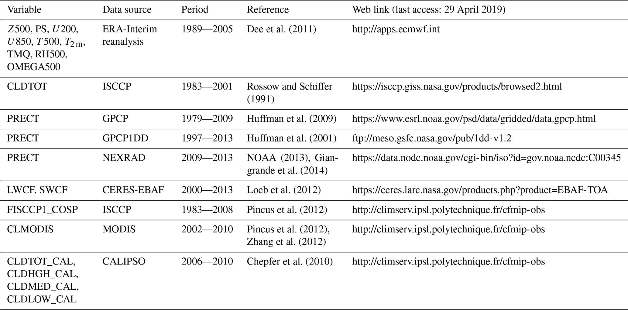
Skillful depictions of the large-scale circulation and sub-grid-scale physics are essential for more realistic model simulations of the atmospheric hydrological cycle. We choose evaluation variables to cover both aspects. Evaluation datasets are summarized in Table 2. Meteorological fields, such as geopotential height, surface pressure, winds, temperature, relative humidity, and precipitable water are from the ERAI reanalysis product (Dee et al., 2011). Seasonal precipitation climatology estimations are based on the Global Precipitation Climatology Project (GPCP) (Huffman et al., 2009). Daily precipitation observations are taken from the GPCP 1∘ daily (1DD) data (Huffman et al., 2001). Hourly precipitation is compared with the dataset collected by the Next-Generation Radar (NEXRAD) network (NOAA, 2013) and developed under the Climate Science for a Sustainable Energy Future (CSSEF) project (Zhang et al., 2005, 2011; Giangrande et al., 2014). Simulated cloud amount is verified against International Satellite Cloud Climatology Project (ISCCP) data (Rossow and Schiffer, 1991). In order to compare with the cloud diagnostics from COSP, we also use the satellite data products generated especially for model evaluation from ISCCP (Pincus et al., 2012; Zhang et al., 2012), Moderate Resolution Imaging Spectroradiometer (MODIS) (Pincus et al., 2012), and Cloud-Aerosol Lidar and Infrared Pathfinder Satellite Observation (CALIPSO) (Chepfer et al., 2010). Top-of-atmosphere cloud radiative effects are evaluated with the Clouds and the Earth's Radiant Energy System–Energy Balanced and Filled (CERES-EBAF v2.8) dataset (Loeb et al., 2012).
Table 2Summary list of observational and reanalysis-based evaluation datasets for model performance.
In this section, we will focus on the results of June–July–August (JJA) and December–January–February (DJF), the two more extreme seasons at the CONUS in a year when some long-standing systematic model errors are present.
3.1 Overall model performance
Taylor diagrams (Taylor, 2001) offer a concise way of summarizing model performance and comparing different model results. Here we employ Taylor diagrams to demonstrate the performance of a selection of important variables (Gleckler et al., 2016). Figure 2 shows the JJA and DJF model climatology of selected thermodynamically related variables (numbered) over the CONUS domain (i.e., the blue box in Fig. 1b) of the RRM grids. Green dots denote LRM results, whereas red dots indicate HRM results and blue dots RRM results with the HRM parameters. The model results are illustrated relative to the verification data (marked by the reference point (1, 0)) described in Sect. 2.2. To make consistent comparisons between different model resolutions, model results are conservatively interpolated (with the “conserve” method of the Earth System Modeling Framework, ESMF, https://www.earthsystemcog.org/projects/esmf/, last access: 1 May 2019, regridding software) to the coarser verification data grids before calculating the Taylor statistics. The radial axis shows the geographic variability (i.e., standard deviation, SD) in the model climatology normalized by that in the observations. The angular axis indicates the spatial correlation (i.e., Pearson correlation coefficient, r) between the simulations and the observations. By design, the distance to the reference point (1, 0) represents the centered root-mean-square (rms) difference between the simulated and observed patterns normalized by the SD of the observations. The closer the distance to the (1, 0) point, the better the model performance. We should note that the primary purpose of our analysis is to show how well the RRM, as an analogue to the HRM, reproduces the HRM results. The observations and the LRM results provide quantitative references to examine the RRM–HRM similarity and also identify poorly simulated behaviors as targets of HRM development.
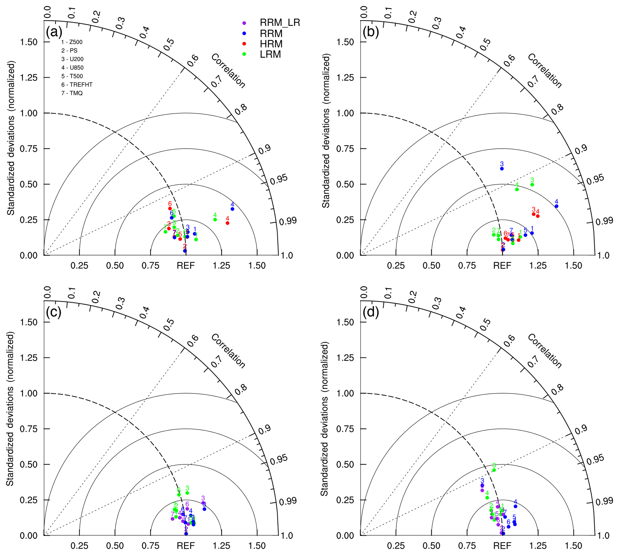
Figure 2Taylor diagrams for three different model climatologies (color-coded: green – LRM; red – HRM; blue – RRM; and purple – RRM_LR) in JJA (a, c) and DJF (b, d). Results are from the CONUS domain (the blue box in Fig. 1b). For panels (a) and (b), verification data are used as the reference point (1, 0), and statistics are calculated on the coarser verification grids. For panels (c) and (d), the HRM is the reference, and statistics are calculated on the HRM grids. The numbers represent the following: 1 – 500 hPa geopotential height (Z500); 2 – surface pressure (PS); 3 – 200 hPa zonal wind (U200); 4 – 850 hPa zonal wind (U850); 5 – 500 hPa temperature (T500); 6 – 2 m air temperature (TREFHT or T2 m); and 7 – total precipitable water (TMQ).
Relative to the evaluation datasets (Fig. 2a, b), the thermodynamic variables are generally well-simulated by EAMv1 with all three model configurations. All correlation coefficients are greater than 0.85 (mostly >0.95). Normalized SDs lie close to the 1.0 dashed curve, especially in JJA. The model generally represents these large-scale circulation related quantities better with finer-resolution settings, as the red dots (HRM) are usually closer to the (1, 0) point (representing evaluation data) than the corresponding green dots (LRM). Nevertheless, there are a few exceptions, for example, 2 m air temperature (T2 m or TREFHT, reference height temperature) in JJA (see Fig. 2a), which is likely associated with cloud and thus surface radiation changes (Van Weverberg et al., 2018) along with feedbacks (surface energy partitioning shifting towards more sensible heat flux) from the land surface model.
More importantly, when using the HRM as the reference point (Fig. 2c, d), blue dots (RRM) are located closer to (1, 0) than the green dots (LRM), indicating that the RRM mimics the HRM behaviors quite well. Additionally, we plot the RRM_LR results (purple dots) on Fig. 2c, d to illustrate the potential impact of poor scale awareness, which is a common problem for current climate models, on conventional RRM applications. Lacking the tuned HRM parameters, previous RRM studies often rely heavily on LRM parameters and cannot quantify the likely performance deterioration due to the parameter–resolution mismatch. Here we take advantage of having both LR and HR tuned parameters to show the parameter influence on RRM performance. As expected, RRM_LR is generally less satisfactory than RRM in matching the HRM behaviors (Fig. 2c, d), but the extent varies for different quantities. For instance, the 200 hPa zonal wind (U200) is relatively insensitive to parameter changes in RRM configurations in both seasons. These results reflect the large-scale nature of upper-troposphere wind fields. In contrast to U200, RRM total precipitable water (TMQ) shows greater sensitivity to parameter settings, since it is more closely related to sub-grid-scale physical processes. These results suggest that RRM generally does well in representing large-scale thermodynamical behaviors of HRM, but some quantities are sensitive to the choice of LRM or HRM parameter settings. A retuning may be needed for the refined region to optimize performance when model physical parameterizations are scale-sensitive. Specifically, for EAMv1, using the HRM parameter setting is recommended when one utilizes the RRM capability.
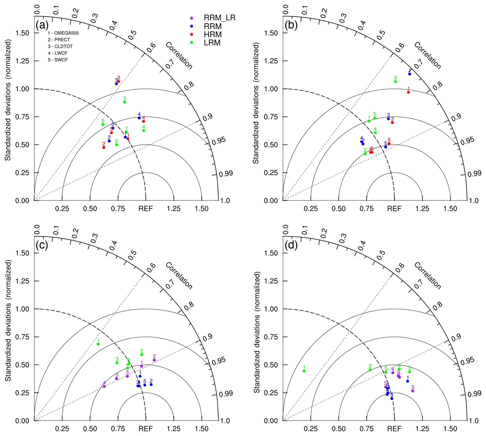
Figure 3Same as Fig. 2, but the numbers represent the following: 1 – 500 hPa vertical velocity (OMEGA500); 2 – total precipitation (PRECT); 3 – vertically integrated total cloud fraction (CLDTOT); 4 – longwave cloud forcing (LWCF); and 5 – shortwave cloud forcing (SWCF).
Compared to thermodynamics variables in Fig. 2, the cloud and precipitation variables in Fig. 3 are more sensitive to sub-grid-scale parameterizations (e.g., convection, cloud microphysics, and radiation). Similar to Bacmeister et al. (2014), the variables in Fig. 3 are more poorly simulated than those in Fig. 2 in all configurations: they have weaker (0.5–0.9) correlation coefficients and are further from the (1, 0) point in both seasons (Fig. 3a, b). These results are consistent with the idea that improving the simulation of these variables requires both better-resolved large-scale circulations and improved representation of physical processes by better physical parameterizations. Figure 3c, d demonstrate this idea quantitatively: the LRM–HRM differences become smaller for all variables after refining the CONUS grids (green to purple); the differences are further reduced by changing the parameters to match the HRM values (purple to blue). Nevertheless, our findings are similar: when increasing the resolution, model performance is generally better in DJF (Fig. 3b) and remains the same or slightly degraded in JJA (Fig. 3a); the RRM results follow those of the HRM closer than do the LRM in both seasons (Fig. 3c, d). In addition, all variables except total precipitation (PRECT) are more sensitive to the resolution change in winter than in summer (greater LRM–HRM separation in Fig. 3b than in Fig. 3a). For example, the variance of 500 hPa vertical velocity (OMEGA500) is almost independent of resolution in summer but about 50 % larger in the HRM configuration than in the LRM in winter, suggesting stronger wintertime circulation and a finer scale of resolved dynamics with the HRM configuration.
These overall Taylor statistics indicate that the RRM simulation with the HR parameters captures the HRM climatological statistics reasonably well, which provide the basis for potential applications of the RRM to effectively test physical parameterizations and simulate regional climate at high resolutions. In the following sections, we will further evaluate the similarity between the RRM and the HR EAMv1 simulations. We will examine some variables that are closely related to the atmospheric hydrologic cycle with a primary focus on detailed aspects of precipitation, which remains a significant challenge in current climate models and is a major focus application for E3SM.
3.2 Regional geographic patterns
In this section we study whether RRMs can reproduce the regional geographic patterns of hydrologic variables simulated by HRM.
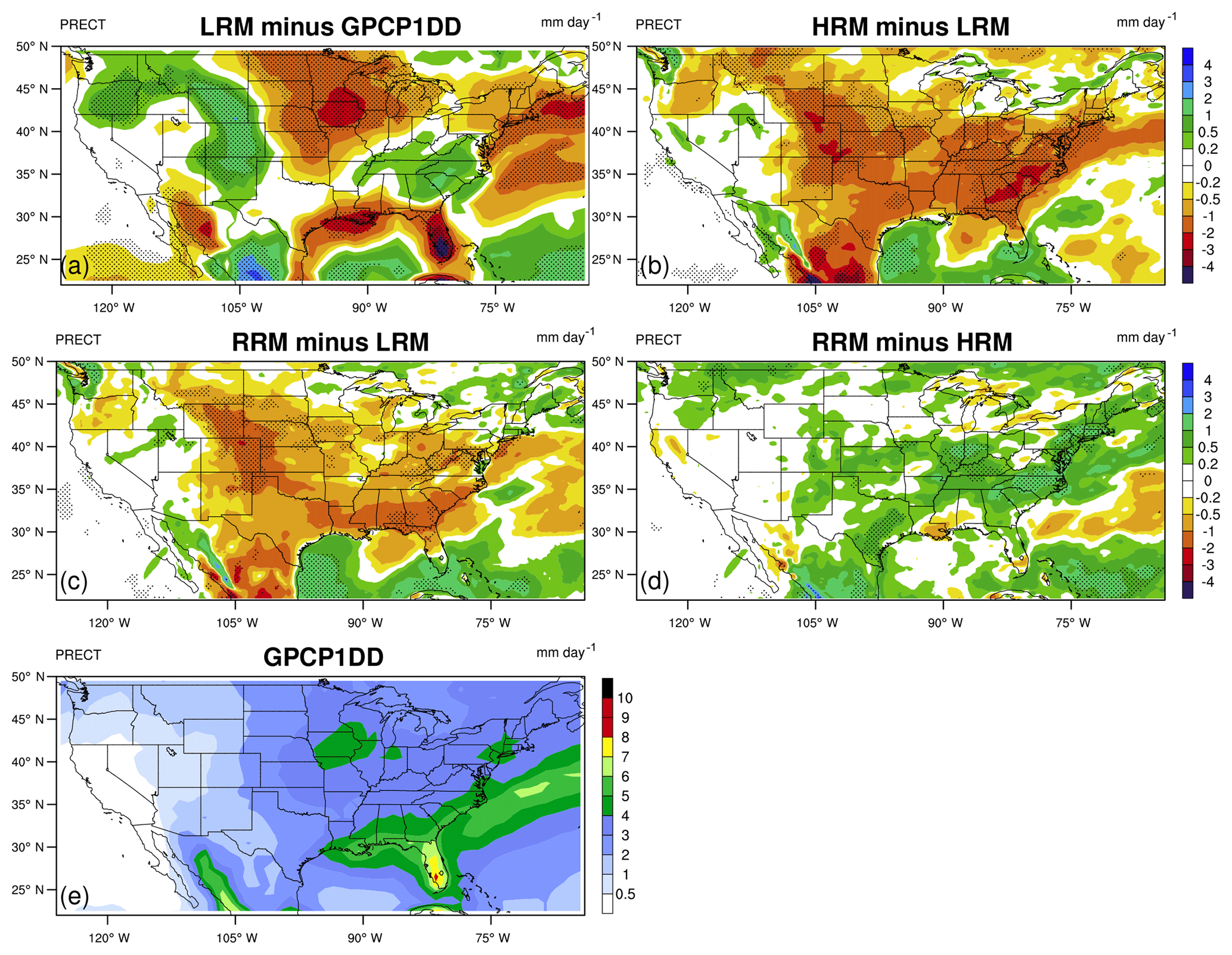
Figure 4Mean differences of total precipitation (unit: mm d−1) in JJA for (a) LRM minus GPCP1DD data, (b) HRM minus LRM, (c) RRM minus LRM, (d) RRM minus HRM, and (e) GPCP1DD. The differences between the LRM and evaluation data (i.e., panel a) are computed on the evaluation grid, while those between models (i.e., panels b–d) are computed on the HRM grid. Dotted areas denote where the differences are statistically significant at the 95 % confidence level with the two-tailed Student's t test.
3.2.1 Precipitation
Figure 4 shows the geographic pattern of mean total (large-scale + convective) precipitation differences between LRM and GPCP1DD observations and the differences among model configurations over the CONUS domain in JJA. The differences between the LRM and evaluation data (i.e., panel a) are computed on the evaluation data grid, while those between models (i.e., panels b–d) are computed on the HRM grid. Dotted regions mark where the differences are statistically significant at a 95 % confidence level with the two-tailed Student's t test assuming that each year is an independent sample. EAMv1 global precipitation results are described by Xie et al. (2018). Compared to GPCP1DD observations, the LRM mostly overestimates (up to 3 mm d−1) western US precipitation and underestimates (up to 4 mm d−1) eastern and central US precipitation (Fig. 4a). As implied by the similar correlation coefficients of precipitation in Fig. 3a, the mean precipitation pattern exhibits rather uniform spatial changes (especially over land) among different model configurations (Fig. 4b–d). Over land, the HRM and RRM typically produce less precipitation than the LRM (partially due to the model tuning, not shown) and the HRM rains the least. Differences between the RRM and the HRM are largely insignificant. In regions that pass the significance test, the differences are also relatively small, for instance, <1 mm d−1 in the southern central US and <2 mm d−1 in the eastern US.
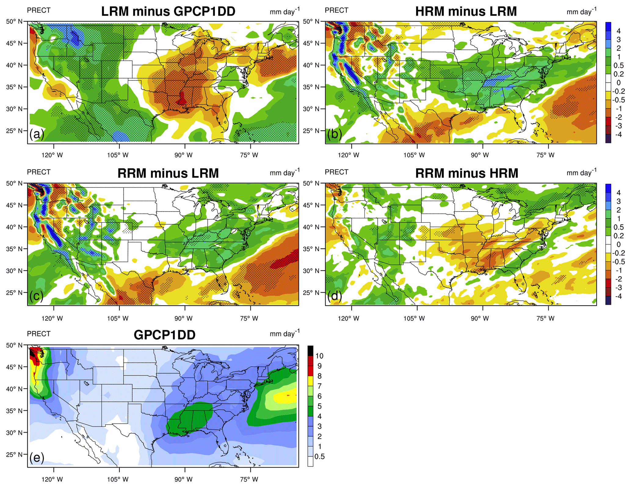
Figure 5 shows the differences in precipitation climatology patterns for DJF. An obvious change from the JJA results in Fig. 4 is the topographic signatures in differences between HRM and LRM (Fig. 5b) and RRM and LRM (Fig. 5c) over mountain regions in the western US, which are associated with better-resolved topography in the RRM and HRM simulations. In addition, the signs of model differences (Fig. 5b–d) are less uniform in DJF than in JJA. Nevertheless, mean precipitation differences between the RRM and the HRM are also small (within ±2 mm d−1) and not statistically significant over most grid cells. Overall, the RRM and HRM EAMv1 produce very similar mean precipitation geographic patterns in both seasons.
Following the COSP evaluation method described by Zhang et al. (2019), cloud fields (not shown here) from the LRM, HRM, and RRM are compared with the observations from ISCCP, MODIS, and CALIPSO. In JJA, all model configurations generally underestimate total cloud amount relative to CALIPSO observations over the CONUS. High thick (optical depth >9.4) clouds lessen with enhanced horizontal resolution over the western central US, matching the precipitation change pattern over the same region in Fig. 4a. Low clouds along the western coast over the ocean increase noticeably in the RRM and HRM compared to the LRM. In DJF, a greater reduction of cloud amount occurs at all levels at the western central US than in JJA with increased resolution. In both seasons, similar to precipitation, the RRM–HRM cloud differences are generally smaller than those for HRM–LRM.
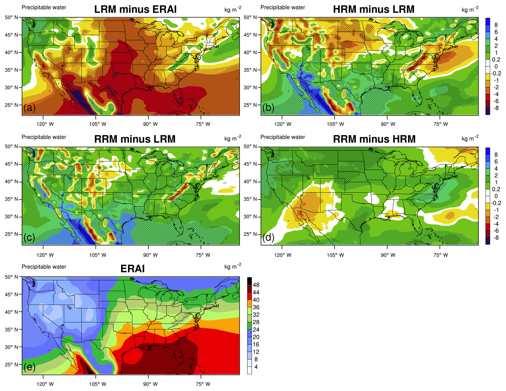
3.2.2 Precipitable water
Figures 6 and 7 show the seasonal mean TMQ in JJA and DJF compared with the ERAI reanalysis data. The LRM underestimates the JJA TMQ over most places (see Fig. 6a) except the northwest US and smaller areas of the eastern US and Mexico, where we observe significantly overestimated precipitation in Fig. 4a. As suggested by the improvement of precipitation with increasing resolution in Fig. 2, the LRM underestimation is generally improved in the HRM (Fig. 6b) and the RRM (Fig. 6c). The mean RRM–HRM differences (Fig. 6d) are mostly positive (<4 kg m−2). This is due to reduction in precipitation in RRM than in HRM outside of CONUS, where the RRM resolution is coarser than that of the HRM.
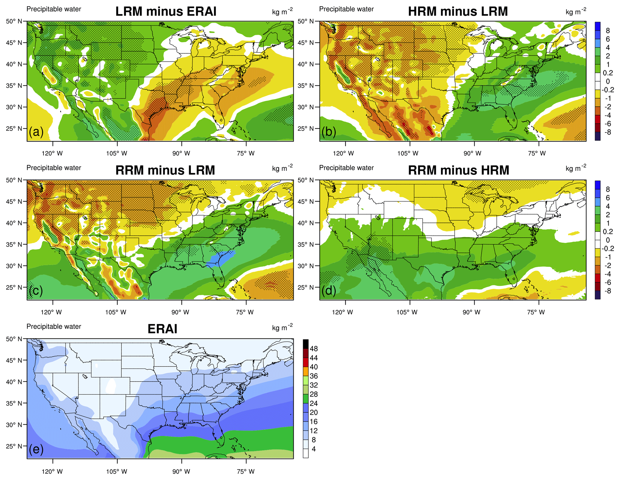
In DJF, the LRM TMQ (Fig. 7a) resembles the patterns (overestimation over the western US and underestimation over the eastern US) of precipitation (Fig. 5a) against evaluation data. Such similarity implies that the precipitation biases in winter are directly related to flaws in precipitable water. The RRM and the HRM differ less (mostly statistically insignificant, see Fig. 7d) than their differences with the LRM (Fig. 7b, c).
3.2.3 Low-level circulation
The low-level jet (LLJ) over the Great Plains of the US has a significant impact on precipitation primarily in summer (Higgins et al., 1997; Pu and Dickinson, 2014). It is responsible for transporting about one-third of the moisture from the Gulf of Mexico to the central US (Helfand and Schubert, 1995). Based on reanalysis data, Higgins et al. (1997) reported connections between the Great Plains LLJ events and regional precipitation anomalies in summer, such as greater precipitation over the north central US and Great Plains and declining precipitation along the Gulf coast and east coast. Here, we examine the 850 hPa horizontal wind speed (Figs 8 and 9; the difference vectors are shown by colors (magnitudes) and magenta streamlines (directions)) as an example of the low-level circulation.
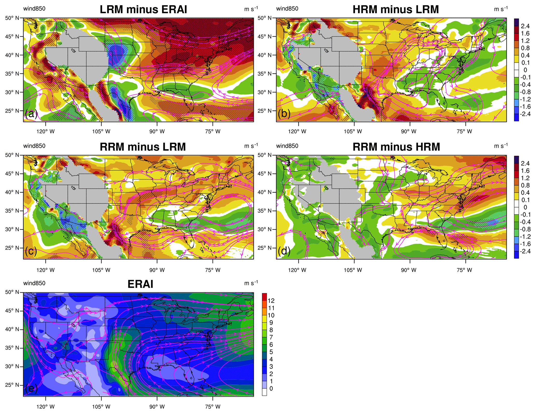
Figure 8Same as Fig. 4, but for 850 hPa wind speed (unit: m s−1) in JJA. The vectors are shown by colors (magnitudes) and magenta streamlines (directions). Grid boxes where surface pressure is less than 850 hPa are shaded in gray in the difference plots.
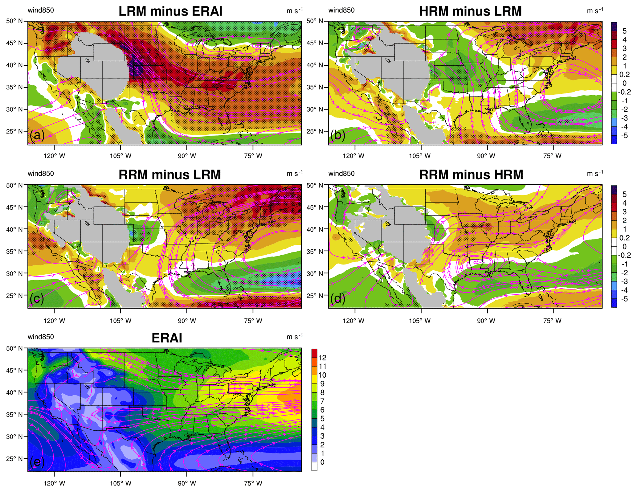
Figure 9Same as Fig. 8, but for DJF. Note that the color scale is different from that in Fig. 8.
In summer, the LRM simulates stronger wind than the ERAI reanalysis over a large portion of CONUS but a weaker southerly LLJ in the central US (see Fig. 8a), which contributes to the low precipitation bias in the Great Plains and along the Gulf coast in Fig. 4a. Enhancing resolution significantly strengthens the LLJ (Fig. 8b, c), consistent with results presented by Berg et al. (2015) for reanalyses with a range of resolutions, and reduces the differences compared to the ERAI reanalysis, since simulations at finer horizontal resolution can resolve the LLJ-related temperature and pressure gradients better than ones at coarser resolution. By contrast, the overestimation of zonal wind strength over the northeastern US becomes slightly worse with finer resolution. The RRM–HRM (Fig. 8d) difference (mostly within ±0.8 m s−1) is generally smaller than that in other panels, especially for the LLJ region over the south central US.
In winter, we find about twice greater wind differences than in summer (note the different color scales in Figs. 8 and 9). However, the main features remain unchanged; for instance, the LRM also simulates zonal winds that were too strong (mostly > 1.0 m s−1) (Fig. 9a), and the RRM–HRM difference is relatively small (within ±2.0 m s−1) and mostly insignificant (Fig. 9d). These results suggest that the RRM mimics the low-level circulation of the HRM, including the summertime LLJ. Together with the precipitable water results in the previous section, they imply similar water vapor transport patterns in the RRM and HRM. Therefore, the RRM is a useful tool to study the HR water transport over CONUS.
3.2.4 Surface air temperature
Warm and dry model biases over the summertime central US have been studied for more than a decade (Klein et al., 2006) and are still deficient in the current generation of regional and global climate models (Cheruy et al., 2014; Mueller and Seneviratne, 2014; Lin et al., 2017; Ma et al., 2018; Morcrette et al., 2018). Land (soil moisture)–atmosphere coupling plays a key role in causing warm and dry biases (Mo and Juang, 2003; Klein et al., 2006; Lin et al., 2017; Ma et al., 2018; Van Weverberg et al., 2018) and the related precipitation biases.
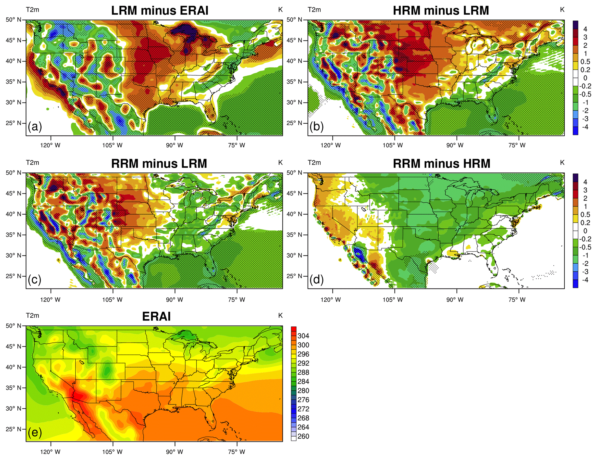
Figure 10 shows the mean JJA patterns of differences in T2 m between the LRM and ERAI data and between three EAMv1 model pairs over CONUS. Over the central US, the LRM simulation exhibits statistically significant positive temperature (up to 3 K) biases throughout the area (see Fig. 10a), corresponding to precipitation low bias (Fig. 4a) in this region. As implied by the Taylor diagram (Fig. 2), performance degrades further (by up to about 4 K) with enhanced resolution. This warm bias can be roughly attributed to two separate sources (Ma et al., 2018): the evaporative fraction (EF) contribution and the radiation contribution which is primarily caused by excessive absorbed solar radiation at the surface. EF is defined as the fraction of the combined latent and sensible heat fluxes that are in latent form. Models with too low an EF tend to use the radiative input to heat the surface instead of evaporating water. The larger bias in the HRM is because the EF contribution is a few times larger with enhanced resolution, while the radiation contribution remains almost unchanged. The noisy and large differences in Fig. 10b, c over western and central mountain regions are likely associated with topographic differences at different resolutions. Figure 10d shows that the RRM–HRM differences are small (<2 K) and statistically not significant but robustly positive over the west coast and negative elsewhere.
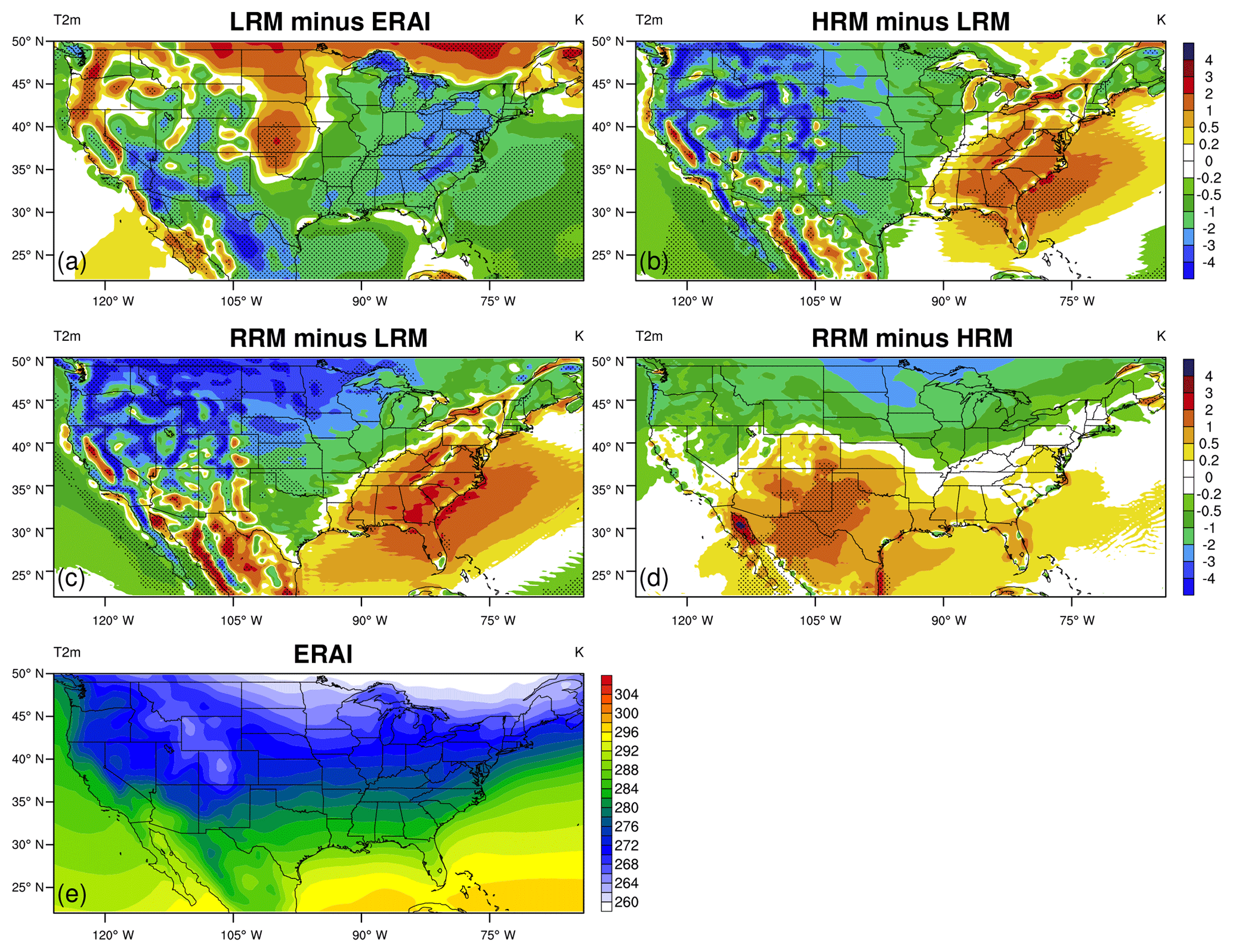
Figure 11 shows the T2 m results in DJF. The LRM (Fig. 11a) still suffers from warm bias over the central US, but it is less severe and much less widespread than in JJA. Over almost the entire eastern US, the LRM underestimates (by up to 4 K) T2 m. The HRM (Fig. 11b) and RRM (Fig. 11c) simulations appear better than the LRM over the Great Plains, the north central US, and the southeastern US. The RRM–HRM differences in Fig. 11d are again the smallest among all panels and statistically insignificant except for the southwestern US.
So far, we have demonstrated that the RRM capability reproduces the characteristics of hydrologic fields simulated in HRM. This proves that the RRM is a reliable test bed which can be used to effectively study and understand these model biases. Next, we will present further analysis of precipitation with RRM and compare it with HRM. Note that the hydrological cycle is a major focus of E3SM of which precipitation is the most important atmospheric variable.
3.3 Precipitation characteristics
3.3.1 Partitioning between large-scale vs. convective precipitation
Precipitation in climate models (e.g., EAMv1) consists of large-scale and convective components. Large-scale precipitation results from condensation due to resolved processes at the model grid resolution and is simulated by the microphysics scheme, while the convective precipitation results from unresolved sub-grid-scale processes that are approximated by the deep convection parameterization. Poor partitioning between these two components manifests itself as errors in the vertical structure of latent heating which corrupts the dynamical response of the environment to convection. Accurately capturing the partitioning is challenging for climate models, which often overestimate the convective component (Lin et al., 2013; Yang et al., 2013). Thus, the partitioning between the large-scale and convective precipitation is an important evaluation metric for climate models. Although they can be clearly defined in the model, the two precipitation components are difficult to separate observationally in a manner comparable to the model. Thus, we only plot the model results for the ratio.
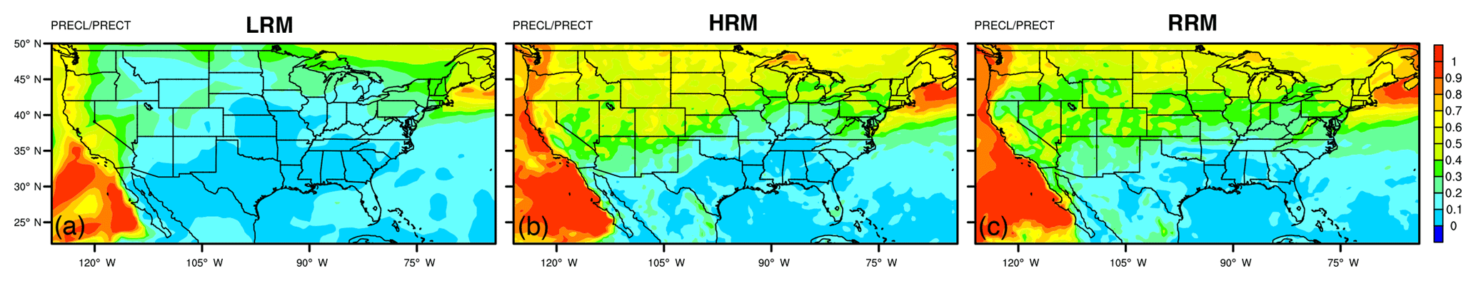
Figure 12Mean ratio of large-scale to total precipitation in JJA for (a) LRM, (b) HRM, and (c) RRM.
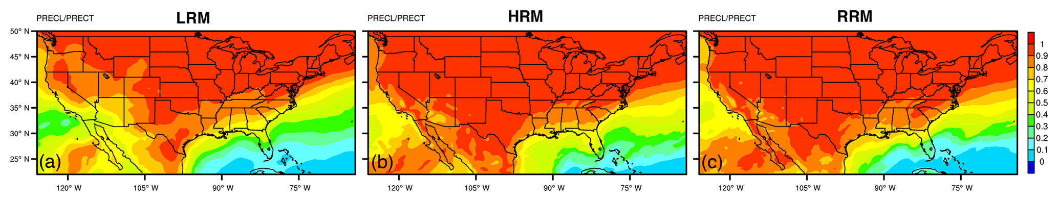
Figures 12 and 13 display the mean ratio of large-scale to total precipitation from EAMv1 models in JJA and DJF, respectively. As expected, convection is a more important source of precipitation in summer and at lower latitudes. The ratio of the large-scale precipitation increases with resolution in Figs. 12 and 13 because more precipitation can be resolved with finer-resolution grids and thus classified as large-scale precipitation. Similar convective precipitation changes with resolution are reported by Bacmeister et al. (2014) for CAM4 and CAM5. Consequently, compared to the LRM, large-scale precipitation in the HRM and RRM is more prevalent (especially in the north) during the summer months (see Fig. 12b, c) and is even more dominant during the winter months (see Fig. 13b, c). In both seasons, the RRM matches the HRM overall distributions of the precipitation partitioning including some regional details, for example, the contour lines along the Sierra Nevada in California in DJF.
3.3.2 Precipitation intensity distribution
Besides the mean precipitation pattern and partitioning into its large-scale and convective components, it is crucial to accurately represent the precipitation intensity distribution in a changing climate because evidence suggests that extreme events, such as severe storms and flooding, will intensify due to the direct impact of global warming on precipitation (Trenberth, 2011; Seeley and Romps, 2014; Walsh et al., 2014). Like many other global climate models (e.g., Dai, 2006; Stephens et al., 2010; Pendergrass and Hartmann, 2014), Terai et al. (2017) showed that EAMv0 suffers from deficiencies in precipitation intensity over the globe, overestimating the frequency of light to moderate rain compared to the GPCP1DD data.
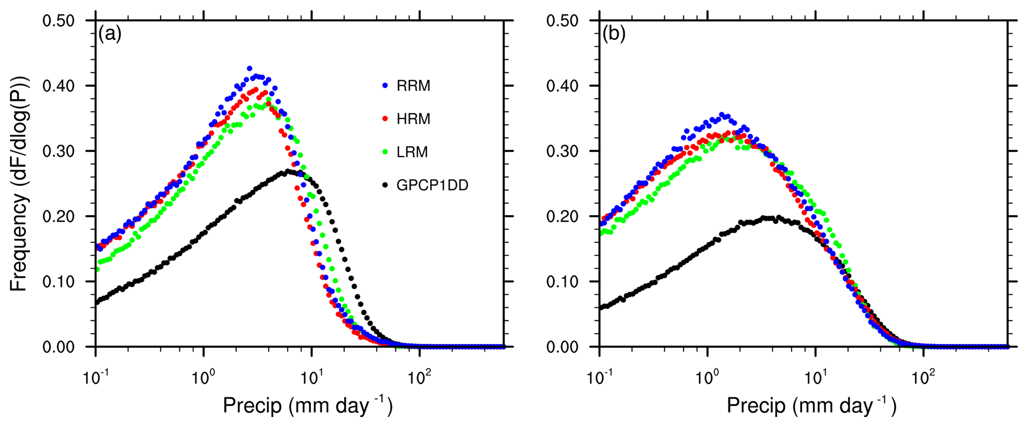
Figure 14Daily mean precipitation frequency (unit: dF∕dlog (P)) functions of total precipitation for the GPCP1DD observation (black), and model simulations: LRM (green), HRM (red), and RRM (blue) in (a) JJA and (b) DJF. Before deriving the distribution, precipitation rates (unit: mm d−1) are interpolated to grids and averaged over daily intervals.
Figure 14 shows EAMv1 vs. GPCP1DD intensity functions over CONUS in JJA and DJF. Before aggregating the distribution, modeled precipitation rates are interpolated with the ESMF conservative regridding method to the same grids as GPCP1DD data. All datasets are averaged over daily intervals. The frequency is then counted in log bins of precipitation rates on each grid. In this way, the frequency functions from datasets at different spatial and temporal resolutions become comparable. It is evident in Fig. 14 that EAMv1 still simulates excessive light precipitation (<10 mm d−1) with all three configurations in both JJA and DJF. As implied by the mean behaviors in Figs. 12 and 13, convective precipitation accounts for a larger fraction of the total in JJA than in DJF across the whole spectrum (not shown in Fig. 14). Total precipitation from the RRM (blue dots) is closer to the HRM (red dots) than to the LRM (green dots) in most bins. These results suggest that we can use the RRM as a test bed to address issues of intensity statistics over CONUS in the HR configurations of future EAM versions.
3.3.3 Diurnal cycle of summertime precipitation
Representing the correct timing and location of these convection episodes is of critical importance for precipitation prediction and hydrologic research (IPCC, 2012). Doing so requires the ability to capture many different meteorological phenomena. For example, summertime mesoscale convective complexes (MCCs) or systems (MCSs) contribute a significant amount of the total precipitation and play an important role in extreme precipitation events over the central US (Maddox, 1980; Carbone et al., 2002; Ashley et al., 2003; Tuttle and Davis, 2006), while disorganized convection strongly influences precipitation over the southeastern US (Dai et al., 1999; Bacmeister et al., 2014; Rickenbach et al., 2015). The diurnal cycle of precipitation is one important measure of a model's ability to reproduce these phenomena. For example, Bacmeister et al. (2014) used the diurnal cycle of precipitation to diagnose deficiencies in capturing the observed phase of MCSs over the central US in CAM5 with both LR and HR configurations.
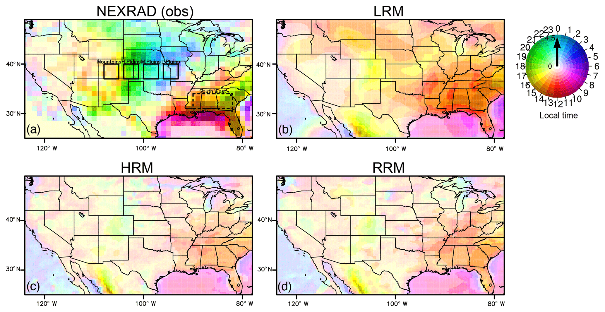
Figure 15Mean diurnal phase (local time; unit: hours) and magnitude (unit: mm d−1) of the maximum precipitation in JJA calculated from the first harmonic for (a) NEXRAD observations, (b) LRM, (c) HRM, and (d) RRM. The phase is indicated by colors, while the magnitude is indicated by the saturation of the color. In panel (a), the solid boxes denote four central US regions from west to east: mountains (37–40∘N, 105–108∘W), high plains (37–40∘N, 101–104∘W), middle plains (37–40∘N, 97–100∘W), and low plains (37–40∘N, 93–96∘W). The dashed box marks the southeast (31–34∘N, 82–90∘W) regions.
Figure 15 illustrates the mean diurnal phase and magnitude patterns of maximum precipitation in JJA from the NEXRAD data and the EAMv1 simulations. The mean diurnal maximum is determined from the first harmonic of the Fourier series constructed from the hourly precipitation time series in each grid box. The phase (local time) of the maximum is indicated by colors, while the magnitude the saturation of the color. The NEXRAD data (Fig. 15a) show the distinct nocturnal (19:00—04:00 LT, UTC−6 h) peak over the central US. This nocturnal peak has been attributed to the eastward propagation of MCSs originating at the front range of Rocky Mountains in the afternoon (Riley et al., 1987; Dai et al., 1999; Carbone et al., 2002; Jiang et al., 2006; Dirmeyer et al., 2012). Unfortunately, no model configuration is successful at capturing this nighttime maximum. The RRM and HRM diurnal phases are similar and show modest improvement over the LRM in the sense that they have weaker amplitudes (lighter colors in panels c and d than in panel b) of incorrect diurnal cycles. The similarity between RRM and HRM indicates that RRM simulations will be valuable for understanding and addressing this important model bias.

Figure 16Mean JJA composite precipitation diurnal cycle from the NEXRAD and model simulations for the subregions (denoted in Fig. 15): mountains (black lines), high plains (purple lines), middle plains (blue lines), low plains (green lines), and southeast (red dashed lines). Panels represent (a) NEXRAD, (b) LRM, (c) HRM, and (d) RRM. We first calculate the simple mean diurnal cycle from the hourly time series for each grid box. The first and second diurnal harmonics of the mean diurnal cycle – obtained using fast Fourier transform – are retained and adjusted to local time to generate the composite diurnal cycle. The composite lines plotted here are averages of the composite diurnal cycle in each grid box within the subregions.
To evaluate the known eastward propagation feature of the convection in this area, we average the JJA precipitation over four subregions: mountains, high plains, middle plains, and low plains, outlined by solid square boxes on Fig. 15a. Figure 16 shows the mean composite diurnal cycle in these subregions. We first calculate the simple mean diurnal cycle from the hourly time series for each grid box. The first and second diurnal harmonics of the mean diurnal cycle – obtained using fast Fourier transform – are retained and adjusted to local time to generate the composite diurnal cycle. The composite lines plotted in Fig. 16 are averages of the composite diurnal cycle in each grid box within the subregions. In the NEXRAD measurements (Fig. 16a), there is a clear propagating pattern: the maximum emerges over the mountains (black) in the afternoon at 15:00 LT, moves eastward and intensifies across the Great Plains, and reaches the middle (blue) and the low (green) plains in the night at 20:00 and 00:00 LT, respectively. The three EAMv1 simulations (Fig. 16b–d) do not reproduce the convection propagation and miss the nocturnal precipitation peak. Although the HRM and the RRM show better skill than the LRM from the mountains to the high plains, these convective events are not strong enough (smaller magnitudes compared to observations) to sustain propagation further east.
The late afternoon rainfall peak over the southeast US is associated with disorganized convection (Bacmeister et al., 2014), a different mechanism than that over the central US. The red dashed lines in Fig. 16 denote the results for the southeast US. The diurnal cycle over the southeast US is generally well-simulated by the LRM, HRM, and RRM (panels b–d), but the time of peak precipitation is a few hours early, consistent with the experience of other models (Dai et al., 1999; Stratton and Stirling, 2012; Bechtold et al., 2014). More physically based improvements are needed to find a solution to the summertime diurnal cycle issue for precipitation over the CONUS, and the RRM provides an efficient test bed for parameterization testing. Previous studies (e.g., Bechtold et al., 2004, 2014; Stratton and Stirling, 2012) provide possible solutions for this issue of simulating the diurnal cycle of convective precipitation over land by modifying convective trigger procedures, entrainment, and convective closures. Our recent study (Xie et al., 2019) shows substantial improvement in the precipitation diurnal cycle in the LRM by employing a new convective trigger with a dynamic constraint on the convection onset and with the capability of detecting moist instability above the boundary layer. We will apply the RRM test bed to extend the new convective trigger to the HRM and report the results in a future paper. This bias in the diurnal cycle of convection is significantly improved in convection-permitting (horizontal grid spacing <2–4 km) simulations (Prein et al., 2015). The E3SM project is making progress in developing its convection-permitting version (E3SMv4), for which the RRM test bed will be heavily relied on.
Nudging is an effective technique to create quasi-deterministic model realizations of observations for a specific time period. There is increasing use of nudging in climate model development and evaluation of physical parameterizations (e.g., Jeuken et al., 1996; Ghan et al., 2001; Kooperman et al., 2012; Zhang et al., 2014). Since nudging simulations constrain the model states closer to observed meteorological conditions, they facilitate the evaluation of modeled physics during specific meteorological episodes. Therefore, nudging can help advance process-level understanding of physical phenomena and ultimately improve physical parameterizations. This is similar to the hindcast approach (Phillips et al., 2004; Ma et al., 2015) that has been widely used for climate model evaluation. EAMv1 has a built-in nudging capability as part of its physics module. When running the nudged RRM, one has various choices available such as nudging variables, locations, and timescales. In this section, we will provide an example of the value of EAMv1 RRM nudging simulations.
The EAMv1 nudging capability in the physics module allows the relaxation of model state variables (U, V, T, and specific humidity, or a subset thereof) towards analysis or reanalysis data. The nudging strength is determined by a fractional nudging coefficient between 0 and 1, which can be a spatial constant or a spatial variable specified by a Heaviside window function. Following previous findings by Zhang et al. (2014) and Ma et al. (2015), we opt to only nudge horizontal velocities for better cloud and aerosol properties with a 6 h relaxation timescale (see Eq. 1 of Zhang et al., 2014). The nudging coefficient map is shown in Fig. 17. The corresponding nudging parameter settings are documented in Table 3. This non-US nudging setting creates a smooth transition from the strongest nudging (red) over coarser grid points to the weakest nudging (blue) over finer grid points. Running in this mode builds a pseudo-regional model framework in a global model. It gives the simulation more freedom over part of the HR region and reduces the nudging noise due to inconsistency between the model and analysis data over the free-running region for better evaluation of physics over this region.
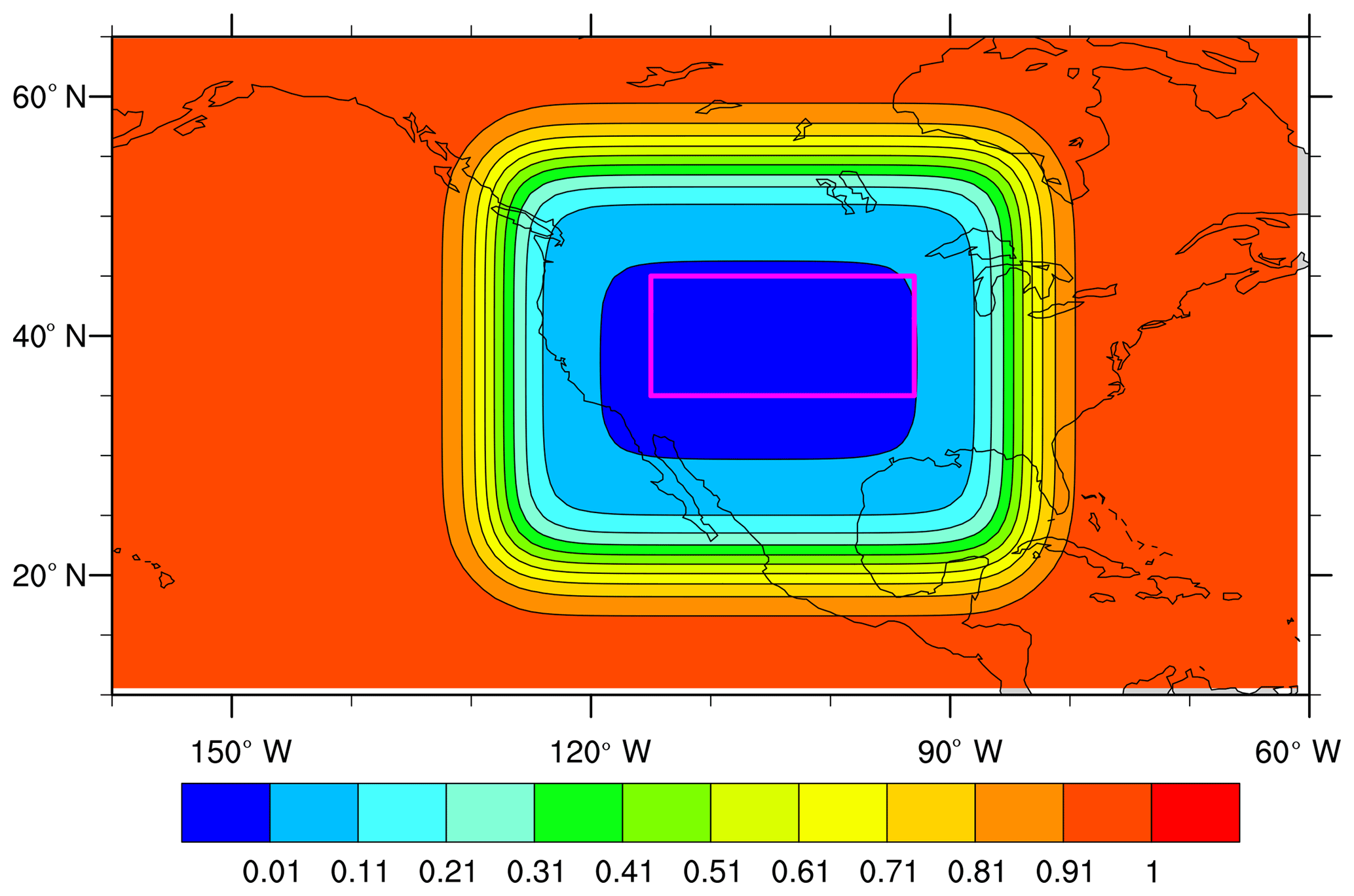
Figure 17Nudging coefficient map zoom-in over North America. A coefficient of 0 indicates that no nudging is applied. The magenta box marks the area of the Hovmöller plots in Fig. 18.
Table 3Nudging parameter settings for the non-US nudging simulation.
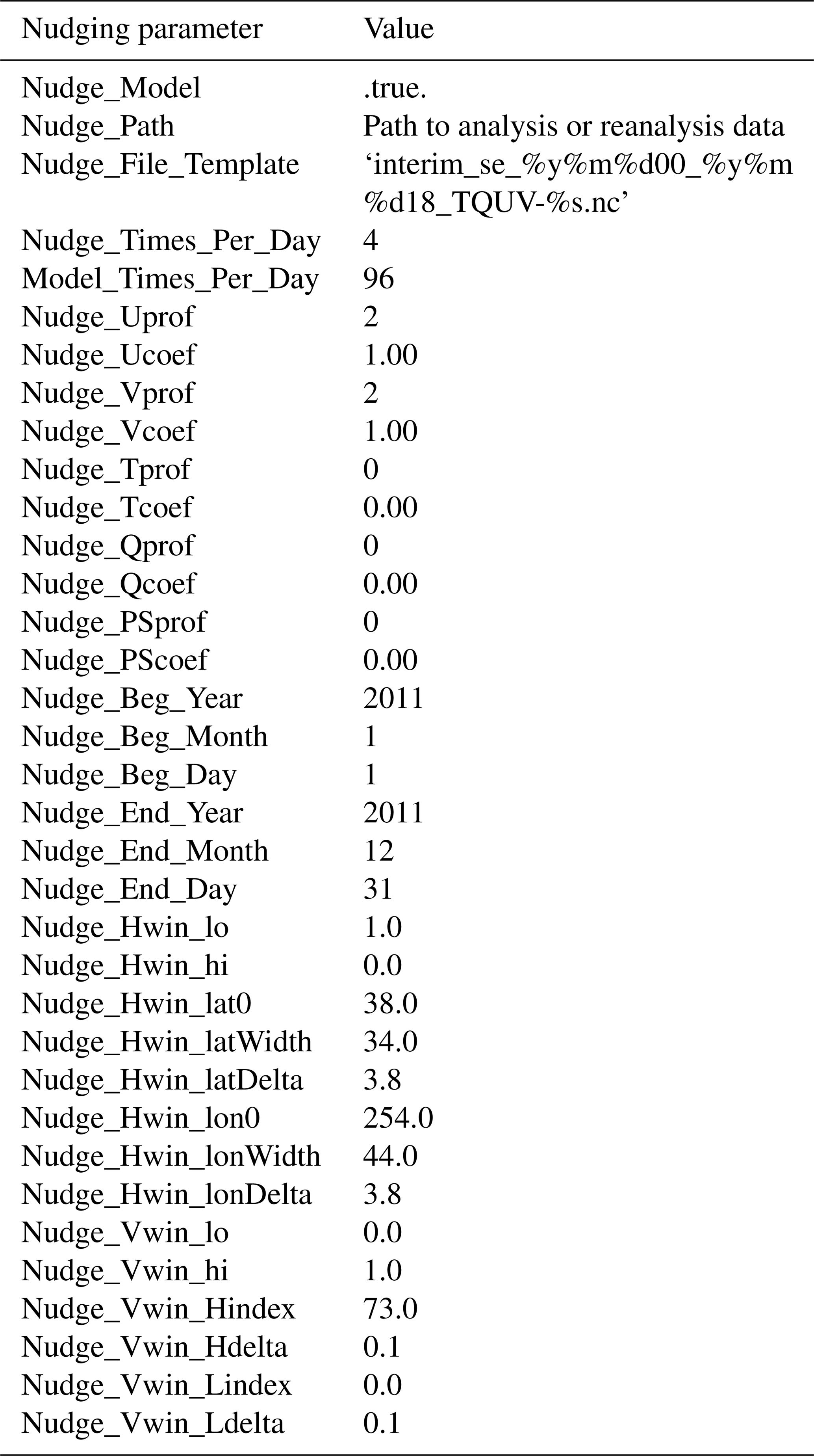
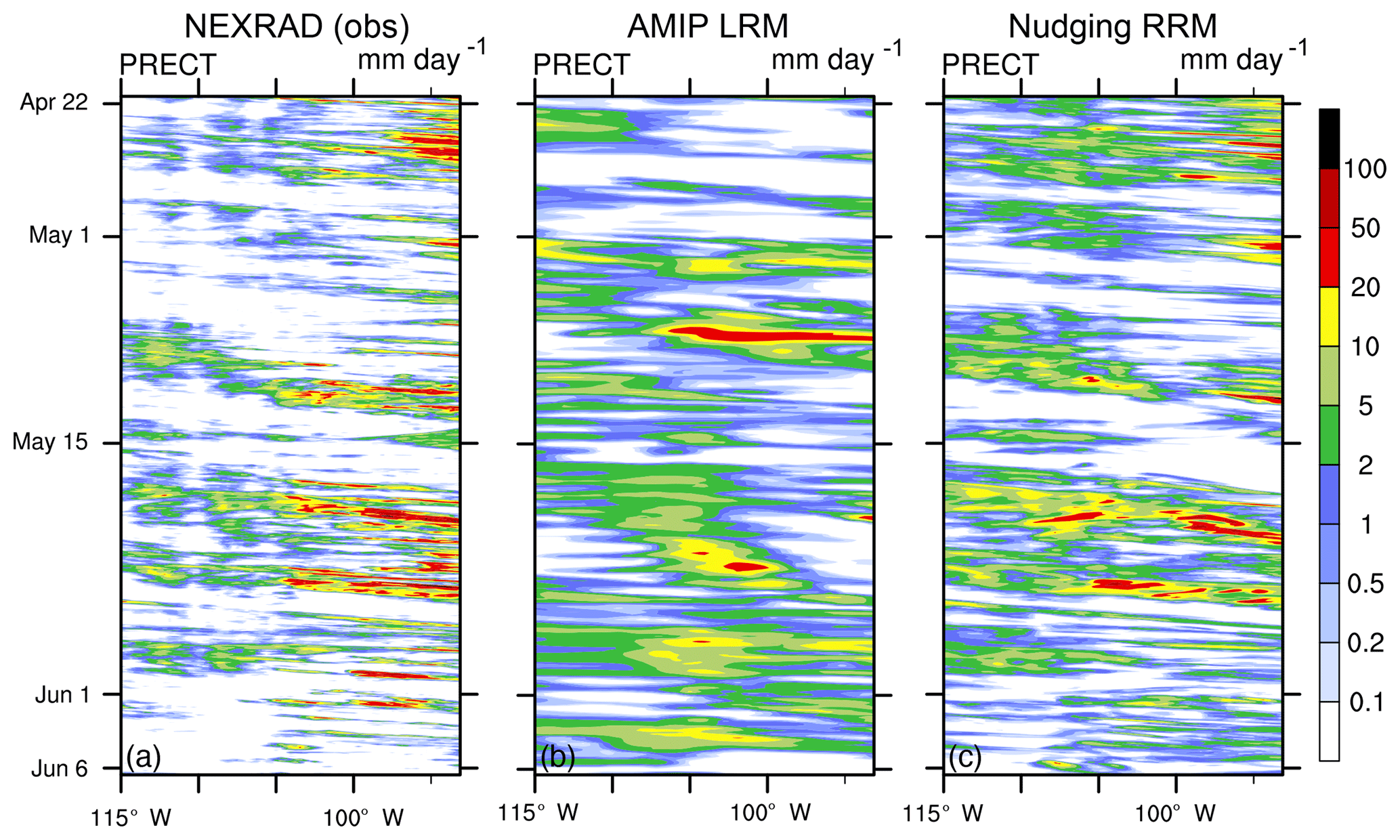
Figure 18Hovmöller plots of hourly mean total precipitation (unit: mm d−1) over 35–45∘N, 93–115∘W during 22 April–6 June 2011 for (a) NEXRAD observations, (b) AMIP LRM, and (c) nudging RRM.
As an example of the nudging results, we create the Hovmöller diagrams (Fig. 18) of hourly mean total precipitation, meridionally averaged over 35–45∘N, 93–115∘W (the magenta box in Fig. 17) during the period of the DOE Atmospheric Radiation Measurement (ARM) Facility's Midlatitude Continental Convective Clouds Experiment (MC3E, 22 April–6 June 2011) (Jensen et al., 2016). The main science goal of the MC3E campaign is to improve the understanding of midlatitude continental convective cloud systems and their interactions with the environment (Xie et al., 2014). Many cloud and precipitation events are observed and clearly shown in the NEXRAD panel (Fig. 18a), such as convective events on 25 April and around 23 May and widespread stratiform rain on 10 May. As expected, the AMIP simulation (Fig. 18b) struggles to capture the statistics of these high-frequency weather systems. The RRM nudging simulation (Fig. 18c) reproduces the timing and location of most events because nudging the horizontal velocities outside of the analyzed area provides more realistic boundary conditions of the large-scale circulation in the free-running domain. There are still some deficiencies in the nudged simulation, for example the incorrect number and propagating speed of convective events, particularly after 15 May. The nudged RRM has cleanly separated these remaining (model-deficiency-based) problems from issues related to the large-scale circulation. This demonstrates that the nudged RRM is an effective test bed for isolating and fixing parameterization problems at resolutions we cannot afford to run globally.
We have presented an overview of the climatological results comparing initial atmosphere-only simulations from globally uniform low resolution (LR, 1∘), high resolution (HR, 0.25∘), and the regionally refined model (RRM, 1 to 0.25∘) over the contiguous US (CONUS) with the atmosphere model version 1 (EAMv1) using the Energy Exascale Earth System Model (E3SM). Our analysis has established that the RRM can generally mimic HR model (HRM) climate behavior over the finely resolved portion (CONUS) for both well-simulated larger-scale thermodynamics fields and less satisfactory smaller-scale physical variables.
Similar to other models (Dai, 2006; Bacmeister et al., 2014), the EAMv1 HRM suffers from deficiencies in convection, clouds, and moist physics (Xie et al., 2018). To verify that the RRM is a suitable alternative framework to the HRM to address these deficiencies, we examine the seasonal mean geographic patterns of precipitation, vertically integrated precipitable water, low-level circulation, and surface temperature for JJA and DJF. Given its key importance in the atmospheric hydrologic cycle, we conduct in-depth analysis on precipitation, including fractions of the large-scale precipitation and daily intensity functions, and the JJA diurnal cycle. Overall, the RRM is similar to the HRM for many finer-scale features, including reproducing long-standing climate model biases, such as a lack of summertime nocturnal precipitation peaks and the warm bias in surface air temperature.
Poor scale awareness of EAMv1 physical parameterizations necessitates retuning the model when increasing resolution. Different from previous RRM work using primarily the LR model (LRM) parameters, we make use of both LRM and HRM parameters and illustrate the significant impact of HR vs. LR parameters on RRM performance due to poor scale awareness, particularly for variables that are closely related to sub-grid-scale physical processes. The high sensitivity of EAMv1 to model resolution suggests the need to develop better scale-aware physical parameterizations or convection-permitting simulations in the future. This study demonstrates how RRMs can be used as a useful test bed to evaluate potentially improved schemes across different spatial scales.
To help users better utilize the E3SM RRM capability, we provide detailed guidance on running the RRM in the nudging mode so that deficiencies in model physical parameterizations can be better isolated. By relaxing the horizontal velocities over coarser-resolution grids to analysis data, we create more realistic boundary conditions to the free-running higher-resolution area. Such a pseudo-regional model framework within a global model displays great advantages in capturing observed convective episodes over the AMIP configuration and hence allows us to calibrate simulated physical processes against observations under different meteorological conditions. With more realistic large-scale circulation conditions, the nudged RRM can be used as a physics test bed for regional process-level studies and aid in the development of future HR EAM versions.
The E3SM source code is available on GitHub: https://github.com/E3SM-Project/E3SM (last access: 2 July 2019; E3SM Project, DOE, 2018).
The E3SM simulation data used in this study can be downloaded at http://portal.nersc.gov/project/acme/tang30/E3SMv1_RRM_CONUS/. The ERA-Interim reanalysis data can be obtained from http://apps.ecmwf.int/. ISCCP cloud amount data are available from https://isccp.giss.nasa.gov/products/browsed2.html. GPCP and GPCP1DD precipitation datasets can be obtained from https://www.esrl.noaa.gov/psd/data/gridded/data.gpcp.html and ftp://meso.gsfc.nasa.gov/pub/1dd-v1.2/. NEXRAD data are available from https://data.nodc.noaa.gov/cgi-bin/iso?id=gov.noaa.ncdc:C00345. CERES-EBAF top-of-atmosphere cloud radiative effects data can be downloaded at https://ceres.larc.nasa.gov/products.php?product=EBAF-TOA. The satellite data for COSP are archived at http://climserv.ipsl.polytechnique.fr/cfmip-obs/.
Table A1EAMv1 simulation setup details.

∗ Used non-default parameter values in Table A2.

| ACME | Accelerated Climate Modeling for Energy |
| AMIP | Atmospheric Model Intercomparison Project |
| ARM | Atmospheric Radiation Measurement |
| CALIPSO | Cloud-Aerosol Lidar and Infrared Pathfinder Satellite Observation |
| CAM | Community Atmosphere Model |
| CERES-EBAF | Clouds and the Earth's Radiant Energy System—Energy Balanced and Filled |
| CESM | Community Earth System Model |
| CLUBB | Cloud Layers Unified By Binormals |
| CONUS | Contiguous United States |
| COSP | Cloud Feedback Model Intercomparison Project Observation Simulator Package |
| CSSEF | Climate Science for a Sustainable Energy Future |
| DJF | December–January–February |
| DOE | Department of Energy |
| E3SM | Energy Exascale Earth System Model |
| EAM | E3SM atmosphere model |
| EF | Evaporative fraction |
| ENA | Eastern North Atlantic |
| ERAI | European Centre for Medium-range Weather Forecasting Interim |
| ESMF | Earth System Modeling Framework |
| GPCP | Global Precipitation Climatology Project |
| GPCP1DD | GPCP 1∘ daily |
| HR | High-resolution |
| HRM | High-resolution model |
| ISCCP | International Satellite Cloud Climatology Project |
| JJA | June–July–August |
| KNL | Knights Landing |
| Linoz | Linearized ozone chemistry |
| LLJ | Low-level jet |
| LR | Low-resolution |
| LRM | Low-resolution model |
| MAM | Modal Aerosol Module |
| MCC | Mesoscale Convective Complex |
| MC3E | Midlatitude Continental Convective Clouds Experiment |
| MCS | Mesoscale convective system |
| MODIS | Moderate Resolution Imaging Spectroradiometer |
| NERSC | National Energy Research Scientific Computing Center |
| NEXRAD | Next-Generation Radar |
| OMEGA500 | 500 hPa vertical velocity |
| PRECT | Total precipitation |
| rms | Root-mean-square |
| RRM | Regionally refined model |
| SD | Standard deviation |
| SST | Sea surface temperature |
| TMQ | Total precipitable water |
| TREFHT | Reference height temperature |
| TWP | Tropical western Pacific |
| U200 | 200 hPa zonal wind |
| US | United States |
| VR | Variable resolution |
QT and SAK designed the experiments. QT and WL performed the simulations and analyzed the data. QT, SAK, and SX designed the scope and structure of the paper. QT prepared the paper with contributions from all coauthors.
The authors declare that they have no conflict of interest.
This research was primarily supported as part of the Energy Exascale Earth System Model (E3SM) project and partially supported by the Climate Model Development and Validation activity, Atmospheric System Research Program, and an earlier project entitled Climate Science for a Sustainable Energy Future, funded by the U.S. Department of Energy (DOE), Office of Science, Office of Biological and Environmental Research (BER) under the auspices of the U.S. DOE by Lawrence Livermore National Laboratory under contract DE-AC52-07NA27344. The Pacific Northwest National Laboratory is operated for DOE by the Battelle Memorial Institute under contract DE-A06-76RLO 1830. This paper has been authored by employees of Brookhaven Science Associates, LLC, under contract no. DE-SC0012704 with the U.S. DOE. The publisher by accepting the paper for publication acknowledges that the U.S. Government retains a nonexclusive, paid-up, irrevocable, world-wide license to publish or reproduce the published form of this paper, or allow others to do so, for U.S. Government purposes. This research used resources of the National Energy Research Scientific Computing Center, a DOE Office of Science User Facility supported by the Office of Science of the U.S. DOE under contract no. DE-AC02-05CH11231. The authors thank Christopher Terai for providing the GPCP1DD data. The authors also thank Jonathan J. Gourley and Zac Flamig of the National Severe Storms Laboratory for access to the archives of NEXRAD NMQ Q2/3 products used in this study. The release number is LLNL-JRNL-764721.
This paper was edited by Patrick Jöckel and reviewed by two anonymous referees.
Ashley, W. S., Mote, T. L., Dixon, P. G., Trotter, S. L., Powell, E. J., Durkee, J. D., and Grundstein, A. J.: Distribution of Mesoscale Convective Complex Rainfall in the United States, Mon. Weather Rev., 131, 3003–3017, https://doi.org/10.1175/1520-0493(2003)131<3003:DOMCCR>2.0.CO;2, 2003.
Bacmeister, J. T., Wehner, M. F., Neale, R. B., Gettelman, A., Hannay, C., Lauritzen, P. H., Caron, J. M., and Truesdale, J. E.: Exploratory High-Resolution Climate Simulations using the Community Atmosphere Model (CAM), J. Climate, 27, 3073–3099, https://doi.org/10.1175/JCLI-D-13-00387.1, 2014.
Bader, D. C., Collins, W., Jacob, R., Jones, P., Rasch, P., Taylor, M., Thornton, P., and Williams, D.: Accelerated Climate Modeling for Energy, available at: https://e3sm.org/wp-content/uploads/2018/03/ACME-project-strategy-July-2014.pdf (last access: 10 January 2019), 2014.
Bechtold, P., Chaboureau, J.-P., Beljaars, A., Betts, A. K., Köhler, M., Miller, M., and Redelsperger, J.-L.: The simulation of the diurnal cycle of convective precipitation over land in a global model, Q. J. Roy. Meteor. Soc., 130, 3119–3137, https://doi.org/10.1256/qj.03.103, 2004.
Bechtold, P., Semane, N., Lopez, P., Chaboureau, J.-P., Beljaars, A., and Bormann, N.: Representing Equilibrium and Nonequilibrium Convection in Large-Scale Models, J. Atmos. Sci., 71, 734–753, https://doi.org/10.1175/JAS-D-13-0163.1, 2014.
Berg, L. K., Riihimaki, L. D., Qian, Y., Yan, H., and Huang, M.: The Low-Level Jet over the Southern Great Plains Determined from Observations and Reanalyses and Its Impact on Moisture Transport, J. Climate, 28, 6682–6706, https://doi.org/10.1175/JCLI-D-14-00719.1, 2015.
Bodas-Salcedo, A., Webb, M. J., Bony, S., Chepfer, H., Dufresne, J.-L., Klein, S. A., Zhang, Y., Marchand, R., Haynes, J. M., Pincus, R., and John, V. O.: COSP: Satellite simulation software for model assessment, B. Am. Meteorol. Soc., 92, 1023–1043, https://doi.org/10.1175/2011BAMS2856.1, 2011.
Bogenschutz, P. A., Gettelman, A., Morrison, H., Larson, V. E., Craig, C., and Schanen, D. P.: Higher-Order Turbulence Closure and Its Impact on Climate Simulations in the Community Atmosphere Model, J. Climate, 26, 9655–9676, https://doi.org/10.1175/JCLI-D-13-00075.1, 2013.
Carbone, R. E., Tuttle, J. D., Ahijevych, D. A., and Trier, S. B.: Inferences of Predictability Associated with Warm Season Precipitation Episodes, J. Atmos. Sci., 59, 2033–2056, https://doi.org/10.1175/1520-0469(2002)059<2033:IOPAWW>2.0.CO;2, 2002.
Chepfer, H., Bony, S., Winker, D., Cesana, G., Dufresne, J. L., Minnis, P., Stubenrauch, C. J., and Zeng, S.: The GCM-Oriented CALIPSO Cloud Product (CALIPSO-GOCCP), J. Geophys. Res., 115, D00H16, https://doi.org/10.1029/2009JD012251, 2010.
Cheruy, F., Dufresne, J. L., Hourdin, F., and Ducharne, A.: Role of clouds and land-atmosphere coupling in midlatitude continental summer warm biases and climate change amplification in CMIP5 simulations, Geophys. Res. Lett., 41, 6493–6500, https://doi.org/10.1002/2014GL061145, 2014.
Dai, A.: Precipitation Characteristics in Eighteen Coupled Climate Models, J. Climate, 19, 4605–4630, https://doi.org/10.1175/JCLI3884.1, 2006.
Dai, A., Giorgi, F., and Trenberth, K. E.: Observed and model-simulated diurnal cycles of precipitation over the contiguous United States, J. Geophys. Res.-Atmos., 104, 6377–6402, https://doi.org/10.1029/98JD02720, 1999.
Dee, D. P., Uppala, S. M., Simmons, A. J., Berrisford, P., Poli, Kobayashi, S., Andrae, U., Balmaseda, M. A., Balsamo, G., Bauer, P., Bechtold, P., Beljaars, A. C. M., van de Berg, L., Bidlot, J., Bormann, N., Delsol, C., Dragani, R., Fuentes, M., Geer, A. J., Haimberger, L., Healy, S. B., Hersbach, H., Hólm, E. V., Isaksen, L., Kållberg, P., Köhler, M., Matricardi, M., McNally, A. P., Monge-Sanz, B. M., Morcrette, J.-J., Park, B.-K., Peubey, C., de Rosnay, P., Tavolato, C., Thépaut, J.-N., and Vitart, F.: The ERA-Interim reanalysis: configuration and performance of the data assimilation system, Q. J. Roy. Meteor. Soc., 137, 553–597, https://doi.org/10.1002/qj.828, 2011.
Dennis, J. M., Edwards, J., Evans, K. J., Guba, O., Lauritzen, P. H., Mirin, A. A., St-Cyr, A., Taylor, M. A., and Worley, P. H.: CAM-SE: A scalable spectral element dynamical core for the Community Atmosphere Model, Int. J. High Perform. C., 26, 74–89, https://doi.org/10.1177/1094342011428142, 2012.
Dirmeyer, P. A., Cash, B. A., Kinter, J. L., Jung, T., Marx, L., Satoh, M., Stan, C., Tomita, H., Towers, P., Wedi, N., Achuthavarier, D., Adams, J. M., Altshuler, E. L., Huang, B., Jin, E. K., and Manganello, J.: Simulating the diurnal cycle of rainfall in global climate models: resolution versus parameterization, Clim. Dynam., 39, 399–418, https://doi.org/10.1007/s00382-011-1127-9, 2012.
E3SM Project, DOE: Energy Exascale Earth System Model, Computer Software, https://doi.org/10.11578/E3SM/dc.20180418.36, 2018.
Fournier, A., Taylor, M. A., and Tribbia, J. J.: The Spectral Element Atmosphere Model (SEAM): High-Resolution Parallel Computation and Localized Resolution of Regional Dynamics, Mon. Weather Rev., 132, 726–748, https://doi.org/10.1175/1520-0493(2004)132<0726:TSEAMS>2.0.CO;2, 2004.
Gettelman, A. and Morrison, H.: Advanced Two-Moment Bulk Microphysics for Global Models. Part I: Off-Line Tests and Comparison with Other Schemes, J. Climate, 28, 1268–1287, https://doi.org/10.1175/JCLI-D-14-00102.1, 2015.
Gettelman, A., Callaghan, P., Larson, V. E., Zarzycki, C. M., Bacmeister, J. T., Lauritzen, P. H., Bogenschutz, P. A., and Neale, R. B.: Regional Climate Simulations With the Community Earth System Model, J. Adv. Model. Earth Syst., 10, 1245–1265, https://doi.org/10.1002/2017MS001227, 2018.
Ghan, S., Laulainen, N., Easter, R., Wagener, R., Nemesure, S., Chapman, E., Zhang, Y.. and Leung, R.: Evaluation of aerosol direct radiative forcing in MIRAGE, J. Geophys. Res.-Atmos., 106, 5295–5316, https://doi.org/10.1029/2000JD900502, 2001.
Giangrande, S. E., Collis, S., Theisen, A. K., and Tokay, A.: Precipitation Estimation from the ARM Distributed Radar Network during the MC3E Campaign, J. Appl. Meteorol. Clim., 53, 2130–2147, https://doi.org/10.1175/JAMC-D-13-0321.1, 2014.
Gleckler, P., Doutriaux, C., Durack, P., Taylor, K. E., Zhang, Y., Williams, D., Mason, E., and Servonnat, J.: A more powerful reality test for climate models, Eos Trans. Am. Geophys. Union, 97, https://doi.org/10.1029/2016EO051663, 2016.
Golaz, J.-C., Larson, V. E., and Cotton, W. R.: A PDF-Based Model for Boundary Layer Clouds. Part I: Method and Model Description, J. Atmos. Sci., 59, 3540–3551, https://doi.org/10.1175/1520-0469(2002)059<3540:APBMFB>2.0.CO;2, 2002.
Golaz, J.-C., Caldwell, P. M., Van Roekel, L. P., Petersen, M. R., Tang, Q., Wolfe, J. D., Abeshu, G., Anantharaj, V., Asay-Davis, X. S., Bader, D. C., Baldwin, S. A., Bisht, G., Bogenschutz, P. A., Branstetter, M., Brunke, M. A., Brus, S. R., Burrows, S. M., Cameron-Smith, P. J., Donahue, A. S., Deakin, M., Easter, R. C., Evans, K. J., Feng, Y., Flanner, M., Foucar, J. G., Fyke, J. G., Griffin, B. M., Hannay, C., Harrop, B. E., Hunke, E. C., Jacob, R. L., Jacobsen, D. W., Jeffery, N., Jones, P. W., Keen, N. D., Klein, S. A., Larson, V. E., Leung, L. R., Li, H.-Y., Lin, W., Lipscomb, W. H., Ma, P.-L., Mahajan, S., Maltrud, M. E., Mametjanov, A., McClean, J. L., McCoy, R. B., Neale, R. B., Price, S. F., Qian, Y., Rasch, P. J., Reeves Eyre, J. E. J., Riley, W. J., Ringler, T. D., Roberts, A. F., Roesler, E. L., Salinger, A. G., Shaheen, Z., Shi, X., Singh, B., Tang, J., Taylor, M. A., Thornton, P. E., Turner, A. K., Veneziani, M., Wan, H., Wang, H., Wang, S., Williams, D. N., Wolfram, P. J., Worley, P. H., Xie, S., Yang, Y., Yoon, J.-H., Zelinka, M. D., Zender, C. S., Zeng, X., Zhang, C., Zhang, K., Zhang, Y., Zheng, X., Zhou, T., and Zhu, Q.: The DOE E3SM coupled model version 1: Overview and evaluation at standard resolution, J. Adv. Model. Earth Syst., 11, https://doi.org/10.1029/2018MS001603, accepted, 2019.
Guba, O., Taylor, M. A., Ullrich, P. A., Overfelt, J. R., and Levy, M. N.: The spectral element method (SEM) on variable-resolution grids: evaluating grid sensitivity and resolution-aware numerical viscosity, Geosci. Model Dev., 7, 2803–2816, https://doi.org/10.5194/gmd-7-2803-2014, 2014.
Helfand, H. M. and Schubert, S. D.: Climatology of the Simulated Great Plains Low-Level Jet and Its Contribution to the Continental Moisture Budget of the United States, J. Climate, 8, 784–806, https://doi.org/10.1175/1520-0442(1995)008<0784:COTSGP>2.0.CO;2, 1995.
Higgins, R. W., Yao, Y., Yarosh, E. S., Janowiak, J. E., and Mo, K. C.: Influence of the Great Plains Low-Level Jet on Summertime Precipitation and Moisture Transport over the Central United States, J. Climate, 10, 481–507, https://doi.org/10.1175/1520-0442(1997)010<0481:IOTGPL>2.0.CO;2, 1997.
Hsu, J. and Prather, M. J.: Stratospheric variability and tropospheric ozone, J. Geophys. Res.-Atmos., 114, D06102, https://doi.org/10.1029/2008JD010942, 2009.
Huang, X. and Ullrich, P. A.: The Changing Character of Twenty-First-Century Precipitation over the Western United States in the Variable-Resolution CESM, J. Climate, 30, 7555–7575, https://doi.org/10.1175/JCLI-D-16-0673.1, 2017.
Huffman, G. J., Adler, R. F., Morrissey, M. M., Bolvin, D. T., Curtis, S., Joyce, R., McGavock, B., and Susskind, J.: Global Precipitation at One-Degree Daily Resolution from Multisatellite Observations, J. Hydrometeorol., 2, 36–50, https://doi.org/10.1175/1525-7541(2001)002<0036:GPAODD>2.0.CO;2, 2001.
Huffman, G. J., Adler, R. F., Bolvin, D. T., and Gu, G.: Improving the global precipitation record: GPCP Version 2.1, Geophys. Res. Lett., 36, L17808, https://doi.org/10.1029/2009GL040000, 2009.
IPCC: Managing the Risks of Extreme Events and Disasters to Advance Climate Change Adaptation, A Special Report of Working Groups I and II of the Intergovernmental Panel on Climate Change, edited by: Field, C. B., Barros, V., Stocker, T. F., Qin, D., Dokken, D. J., Ebi, K. L., Mastrandrea, M. D., Mach, K. J., Plattner, G.-K., Allen, S. K., Tignor, M., and Midgley, P. M., Cambridge University Press, Cambridge, UK, and New York, NY, USA, 2012.
Jensen, M. P., Petersen, W. A., Bansemer, A., Bharadwaj, N., Carey, L. D., Cecil, D. J., Collis, S. M., Del Genio, A. D., Dolan, B., Gerlach, J., Giangrande, S. E., Heymsfield, A., Heymsfield, G., Kollias, P., Lang, T. J., Nesbitt, S. W., Neumann, A., Poellot, M., Rutledge, S. A., Schwaller, M., Tokay, A., Williams, C. R., Wolff, D. B., Xie, S., and Zipser, E. J.: The Midlatitude Continental Convective Clouds Experiment (MC3E), B. Am. Meteorol. Soc., 97, 1667–1686, https://doi.org/10.1175/BAMS-D-14-00228.1, 2016.
Jeuken, A. B. M., Siegmund, P. C., Heijboer, L. C., Feichter, J., and Bengtsson, L.: On the potential of assimilating meteorological analyses in a global climate model for the purpose of model validation, J. Geophys. Res.-Atmos., 101, 16939–16950, https://doi.org/10.1029/96JD01218, 1996.
Jiang, X., Lau, N., and Klein, S. A.: Role of eastward propagating convection systems in the diurnal cycle and seasonal mean of summertime rainfall over the U.S. Great Plains, Geophys. Res. Lett., 33, L19809, https://doi.org/10.1029/2006GL027022, 2006.
Klein, S. A., Jiang, X., Boyle, J., Malyshev, S., and Xie, S.: Diagnosis of the summertime warm and dry bias over the U.S. Southern Great Plains in the GFDL climate model using a weather forecasting approach, Geophys. Res. Lett., 33, L18805, https://doi.org/10.1029/2006GL027567, 2006.
Klein, S. A., Zhang, Y., Zelinka, M. D., Pincus, R., Boyle, J., and Gleckler, P. J.: Are climate model simulations of clouds improving? An evaluation using the ISCCP simulator, J. Geophys. Res.-Atmos., 118, 1329–1342, https://doi.org/10.1002/jgrd.50141, 2013.
Kooperman, G. J., Pritchard, M. S., Ghan, S. J., Wang, M., Somerville, R. C. J., and Russell, L. M.: Constraining the influence of natural variability to improve estimates of global aerosol indirect effects in a nudged version of the Community Atmosphere Model 5, J. Geophys. Res.-Atmos., 117, D23204, https://doi.org/10.1029/2012JD018588, 2012.
Lin, Y., Zhao, M., Ming, Y., Golaz, J.-C., Donner, L. J., Klein, S. A., Ramaswamy, V., and Xie, S.: Precipitation Partitioning, Tropical Clouds, and Intraseasonal Variability in GFDL AM2, J. Climate, 26, 5453–5466, https://doi.org/10.1175/JCLI-D-12-00442.1, 2013.
Lin, Y., Dong, W., Zhang, M., Xie, Y., Xue, W., Huang, J., and Luo, Y.: Causes of model dry and warm bias over central U.S. and impact on climate projections, Nat. Commun., 8, 881, https://doi.org/10.1038/s41467-017-01040-2, 2017.
Liu, X., Ma, P.-L., Wang, H., Tilmes, S., Singh, B., Easter, R. C., Ghan, S. J., and Rasch, P. J.: Description and evaluation of a new four-mode version of the Modal Aerosol Module (MAM4) within version 5.3 of the Community Atmosphere Model, Geosci. Model Dev., 9, 505–522, https://doi.org/10.5194/gmd-9-505-2016, 2016.
Loeb, N. G., Lyman, J. M., Johnson, G. C., Allan, R. P., Doelling, D. R., Wong, T., Soden, B. J., and Stephens, G. L.: Observed changes in top-of-the-atmosphere radiation and upper-ocean heating consistent within uncertainty, Nat. Geosci., 5, 110–113, https://doi.org/10.1038/ngeo1375, 2012.
Ma, H.-Y., Xie, S., Klein, S. A., Williams, K. D., Boyle, J. S., Bony, S., Douville, H., Fermepin, S., Medeiros, B., Tyteca, S., Watanabe, M., and Williamson, D.: On the Correspondence between Mean Forecast Errors and Climate Errors in CMIP5 Models, J. Climate, 27, 1781–1798, https://doi.org/10.1175/JCLI-D-13-00474.1, 2014.
Ma, H.-Y., Chuang, C. C., Klein, S. A., Lo, M.-H., Zhang, Y., Xie, S., Zheng, X., Ma, P.-L., Zhang, Y., and Phillips, T. J.: An improved hindcast approach for evaluation and diagnosis of physical processes in global climate models, J. Adv. Model. Earth Syst., 7, 1810–1827, https://doi.org/10.1002/2015MS000490, 2015.
Ma, H.-Y., Klein, S. A., Xie, S., Zhang, C., Tang, S., Tang, Q., Morcrette, C. J., Van Weverberg, K., Petch, J., Ahlgrimm, M., Berg, L. K., Cheruy, F., Cole, J., Forbes, R., Gustafson, W. I., Huang, M., Liu, Y., Merryfield, W., Qian, Y., Roehrig, R., and Wang, Y.-C.: CAUSES: On the Role of Surface Energy Budget Errors to the Warm Surface Air Temperature Error Over the Central United States, J. Geophys. Res.-Atmos., 123, 2888–2909, https://doi.org/10.1002/2017JD027194, 2018.
Maddox, R. A.: Meoscale Convective Complexes, B. Am. Meteorol. Soc., 61, 1374–1387, https://doi.org/10.1175/1520-0477(1980)061<1374:MCC>2.0.CO;2, 1980.
Mo, K. C. and Juang, H. H.: Relationships between soil moisture and summer precipitation over the Great Plains and the Southwest, J. Geophys. Res.-Atmos., 108, 8610, https://doi.org/10.1029/2002JD002952, 2003.
Morcrette, C. J., Van Weverberg, K., Ma, H.-Y., Ahlgrimm, M., Bazile, E., Berg, L. K., Cheng, A., Cheruy, F., Cole, J., Forbes, R., Gustafson, W. I., Huang, M., Lee, W.-S., Liu, Y., Mellul, L., Merryfield, W. J., Qian, Y., Roehrig, R., Wang, Y.-C., Xie, S., Xu, K.-M., Zhang, C., Klein, S., and Petch, J.: Introduction to CAUSES: Description of Weather and Climate Models and Their Near-Surface Temperature Errors in 5 day Hindcasts Near the Southern Great Plains, J. Geophys. Res.-Atmos., 123, 2655–2683, https://doi.org/10.1002/2017JD027199, 2018.
Mueller, B. and Seneviratne, S. I.: Systematic land climate and evapotranspiration biases in CMIP5 simulations, Geophys. Res. Lett., 41, 128–134, https://doi.org/10.1002/2013GL058055, 2014.
Neale, R. B., Chen, C. C., Gettelman, A., Lauritzen, P. H., Park, S., Williamson, D. L., Conley, A. J., Garcia, R., Kinnison, D., Lamarque, J. F., Marsh, D., Mills, M., Smith, A. K., Tilmes, S., Vitt, F., Cameron-Smith, P., Collins, W. D., Iacono, M. J., Easter, R. C., Ghan, S. J., Liu, X., Rasch, P. J., and Taylor, M. A.: Description of the NCAR Community Atmosphere Model (CAM5.0), Tech. Note NCAR/TN-486+STR, 274 pp., available at: http://www.cesm.ucar.edu/models/cesm1.0/cam/docs/description/cam5_desc.pdf (last access: 2 July 2019), 2012.
NOAA: NOAA National Weather Service (NWS) Radar Operations Center (1991): NOAA Next Generation Radar (NEXRAD) Level 2 Base Data. NOAA National Centers for Environmental Information, https://doi.org/10.7289/V5W9574V, 2013.
Pendergrass, A. G. and Hartmann, D. L.: Changes in the Distribution of Rain Frequency and Intensity in Response to Global Warming, J. Climate, 27, 8372–8383, https://doi.org/10.1175/JCLI-D-14-00183.1, 2014.
Phillips, T. J., Potter, G. L., Williamson, D. L., Cederwall, R. T., Boyle, J. S., Fiorino, M., Hnilo, J. J., Olson, J. G., Xie, S., and Yio, J. J.: Evaluating Parameterizations in General Circulation Models: Climate Simulation Meets Weather Prediction, B. Am. Meteorol. Soc., 85, 1903–1915, https://doi.org/10.1175/BAMS-85-12-1903, 2004.
Pincus, R., Platnick, S., Ackerman, S. A., Hemler, R. S., and Patrick Hofmann, R. J.: Reconciling Simulated and Observed Views of Clouds: MODIS, ISCCP, and the Limits of Instrument Simulators, J. Climate, 25, 4699–4720, https://doi.org/10.1175/JCLI-D-11-00267.1, 2012.
Prein, A. F., Langhans, W., Fosser, G., Ferrone, A., Ban, N., Goergen, K., Keller, M., Tölle, M., Gutjahr, O., Feser, F., Brisson, E., Kollet, S., Schmidli, J., van Lipzig, N. P. M., and Leung, R.: A review on regional convection-permitting climate modeling: Demonstrations, prospects, and challenges, Rev. Geophys., 53, 323–361, https://doi.org/10.1002/2014RG000475, 2015.
Pu, B. and Dickinson, R. E.: Diurnal Spatial Variability of Great Plains Summer Precipitation Related to the Dynamics of the Low-Level Jet, J. Atmos. Sci., 71, 1807–1817, https://doi.org/10.1175/JAS-D-13-0243.1, 2014.
Qian, Y., Jackson, C., Giorgi, F., Booth, B., Duan, Q., Forest, C., Higdon, D., Hou, Z. J., and Huerta, G.: Uncertainty Quantification in Climate Modeling and Projection, B. Am. Meteorol. Soc., 97, 821–824, https://doi.org/10.1175/BAMS-D-15-00297.1, 2016.
Qian, Y., Wan, H., Yang, B., Golaz, J.-C., Harrop, B., Hou, Z., Larson, V. E., Leung, L. R., Lin, G., Lin, W., Ma, P.-L., Ma, H.-Y., Rasch, P., Singh, B., Wang, H., Xie, S., and Zhang, K.: Parametric Sensitivity and Uncertainty Quantification in the Version 1 of E3SM Atmosphere Model Based on Short Perturbed Parameter Ensemble Simulations, J. Geophys. Res.-Atmos., 123, 13046–13073, https://doi.org/10.1029/2018JD028927, 2018.
Rasch, P., Xie, S., Ma, P.-L., Lin, W., Wang, H., Tang, Q., Burrows, S., Caldwell, P., Zhang, K., Easter, R., Cameron-Smith, P., Singh, B., Wan, H., Golaz, J.-C., Harrop, B., Roesler, E., Bacmeister, J., Larson, V., Evans, K., Qian, Y., Taylor, M., Leung, R., Zhang, Y., Brent, L., Branstettor, M., Hannay, C., Mahajan, S., Mametjanov, A., Neale, R., Richter, J., Yoon, J., Zender, C., Bader, D., Flanner, M., Foucar, J., Jacob, R., Keen, N., Klein, S., Liu, X., Salinger, A., Shrivastava, M., and Yang, Y.: An Overview of the Atmospheric Component of the Energy Exascale Earth System Model, J. Adv. Model. Earth Syst., jame20932, https://doi.org/10.1029/2019MS001629, accepted, 2019.
Reynolds, R. W., Rayner, N. A., Smith, T. M., Stokes, D. C., and Wang, W.: An Improved In Situ and Satellite SST Analysis for Climate, J. Climate, 15, 1609–1625, https://doi.org/10.1175/1520-0442(2002)015<1609:AIISAS>2.0.CO;2, 2002.
Rhoades, A. M., Huang, X., Ullrich, P. A., and Zarzycki, C. M.: Characterizing Sierra Nevada Snowpack Using Variable-Resolution CESM, J. Appl. Meteorol. Clim., 55, 173–196, https://doi.org/10.1175/JAMC-D-15-0156.1, 2016.
Rickenbach, T. M., Nieto-Ferreira, R., Zarzar, C., and Nelson, B.: A seasonal and diurnal climatology of precipitation organization in the southeastern United States: Precipitation Organization in Southeastern USA, Q. J. Roy. Meteor. Soc., 141, 1938–1956, https://doi.org/10.1002/qj.2500, 2015.
Riley, G. T., Landin, M. G., and Bosart, L. F.: The Diurnal Variability of Precipitation across the Central Rockies and Adjacent Great Plains, Mon. Weather Rev., 115, 1161–1172, https://doi.org/10.1175/1520-0493(1987)115<1161:TDVOPA>2.0.CO;2, 1987.
Ringler, T., Ju, L., and Gunzburger, M.: A multiresolution method for climate system modeling: application of spherical centroidal Voronoi tessellations, Ocean Dynam., 58, 475–498, https://doi.org/10.1007/s10236-008-0157-2, 2008.
Roesler, E., Taylor, M. A., Tang, Q., and Lin, W.: Climatology of the Exascale Energy Earth System Model's Atmospheric Model, version 0, Configured with Variable Resolution over the Continental United States, Theor. Appl. Climatol., under review, 2019.
Rossow, W. B. and Schiffer, R. A.: ISCCP Cloud Data Products, B. Am. Meteorol. Soc., 72, 2–20, https://doi.org/10.1175/1520-0477(1991)072<0002:ICDP>2.0.CO;2, 1991.
Seeley, J. T. and Romps, D. M.: The Effect of Global Warming on Severe Thunderstorms in the United States, J. Climate, 28, 2443–2458, https://doi.org/10.1175/JCLI-D-14-00382.1, 2014.
Stephens, G. L., L'Ecuyer, T., Forbes, R., Gettelmen, A., Golaz, J.-C., Bodas-Salcedo, A., Suzuki, K., Gabriel, P., and Haynes, J.: Dreary state of precipitation in global models, J. Geophys. Res.-Atmos., 115, D24211, https://doi.org/10.1029/2010JD014532, 2010.
Stratton, R. A. and Stirling, A. J.: Improving the diurnal cycle of convection in GCMs, Q. J. Roy. Meteor. Soc., 138, 1121–1134, https://doi.org/10.1002/qj.991, 2012.
Taylor, K. E.: Summarizing multiple aspects of model performance in a single diagram, J. Geophys. Res.-Atmos., 106, 7183–7192, https://doi.org/10.1029/2000JD900719, 2001.
Taylor, M. A. and Fournier, A.: A compatible and conservative spectral element method on unstructured grids, J. Comput. Phys., 229, 5879–5895, https://doi.org/10.1016/j.jcp.2010.04.008, 2010.
Terai, C. R., Caldwell, P. M., Klein, S. A., Tang, Q., and Branstetter, M. L.: The atmospheric hydrologic cycle in the ACME v0.3 model, Clim. Dynam., 1–29, https://doi.org/10.1007/s00382-017-3803-x, 2017.
Trenberth, K. E.: Changes in precipitation with climate change, Clim. Res., 47, 123–138, https://doi.org/10.3354/cr00953, 2011.
Tuttle, J. D. and Davis, C. A.: Corridors of Warm Season Precipitation in the Central United States, Mon. Weather Rev., 134, 2297–2317, https://doi.org/10.1175/MWR3188.1, 2006.
Van Weverberg, K., Morcrette, C. J., Petch, J., Klein, S. A., Ma, H.-Y., Zhang, C., Xie, S., Tang, Q., Gustafson, W. I., Qian, Y., Berg, L. K., Liu, Y., Huang, M., Ahlgrimm, M., Forbes, R., Bazile, E., Roehrig, R., Cole, J., Merryfield, W., Lee, W.-S., Cheruy, F., Mellul, L., Wang, Y.-C., Johnson, K., and Thieman, M. M.: CAUSES: Attribution of Surface Radiation Biases in NWP and Climate Models near the U.S. Southern Great Plains, J. Geophys. Res.-Atmos., 123, 3612–3644, https://doi.org/10.1002/2017JD027188, 2018.
Walsh, J., Wuebbles, D., Hayhoe, K., Kossin, J., Kunkel, K., Stephens, G., Thorne, P., Vose, R., Wehner, M., Willis, J., Anderson, D., Doney, S., Feely, R., Hennon, P., Kharin, V., Knutson, T., Landerer, F., Lenton, T., Kennedy, J., and Somerville, R.: Our Changing Climate, chap. 2, in: Climate Change Impacts in the United States: The Third National Climate Assessment, 19–67, https://doi.org/10.7930/J0KW5CXT, 2014.
Williamson, D. L.: The effect of time steps and time-scales on parametrization suites, Q. J. Roy. Meteor. Soc., 139, 548–560, https://doi.org/10.1002/qj.1992, 2013.
Wu, C., Liu, X., Lin, Z., Rhoades, A. M., Ullrich, P. A., Zarzycki, C. M., Lu, Z., and Rahimi-Esfarjani, S. R.: Exploring a Variable-Resolution Approach for Simulating Regional Climate in the Rocky Mountain Region Using the VR-CESM, J. Geophys. Res.-Atmos., 122, 10939–10965, https://doi.org/10.1002/2017JD027008, 2017.
Xie, S., Ma, H.-Y., Boyle, J. S., Klein, S. A., and Zhang, Y.: On the Correspondence between Short- and Long-Time-Scale Systematic Errors in CAM4/CAM5 for the Year of Tropical Convection, J. Climate, 25, 7937–7955, https://doi.org/10.1175/JCLI-D-12-00134.1, 2012.
Xie, S., Zhang, Y., Giangrande, S. E., Jensen, M. P., McCoy, R., and Zhang, M.: Interactions between cumulus convection and its environment as revealed by the MC3E sounding array, J. Geophys. Res.-Atmos., 119, 11784–11808, https://doi.org/10.1002/2014JD022011, 2014.
Xie, S., Lin, W., Rasch, P. J., Ma, P.-L., Neale, R., Larson, V. E., Qian, Y., Bogenschutz, P. A., Caldwell, P., Cameron-Smith, P., Golaz, J.-C., Mahajan, S., Singh, B., Tang, Q., Wang, H., Yoon, J.-H., Zhang, K., and Zhang, Y.: Understanding Cloud and Convective Characteristics in Version 1 of the E3SM Atmosphere Model, J. Adv. Model. Earth Syst., 10, 2618–2644, https://doi.org/10.1029/2018MS001350, 2018.
Xie, S., Wang, Y.-C., Lin, W., Ma, H.-Y., Tang, Q., Tang, S., Zheng, X., Golaz, J.-C., Zhang, G., and Zhang, M.: Improved Diurnal Cycle of Precipitation in E3SM with a Revised Convective Triggering Function, J. Adv. Model. Earth Syst., 11, https://doi.org/10.1029/2019MS001702, accepted, 2019.
Yang, B., Qian, Y., Lin, G., Leung, L. R., Rasch, P. J., Zhang, G. J., McFarlane, S. A., Zhao, C., Zhang, Y., Wang, H., Wang, M., and Liu, X.: Uncertainty quantification and parameter tuning in the CAM5 Zhang-McFarlane convection scheme and impact of improved convection on the global circulation and climate, J. Geophys. Res.-Atmos., 118, 395–415, https://doi.org/10.1029/2012JD018213, 2013.
Zarzycki, C. M. and Jablonowski, C.: A multidecadal simulation of Atlantic tropical cyclones using a variable-resolution global atmospheric general circulation model, J. Adv. Model. Earth Syst., 6, 805–828, https://doi.org/10.1002/2014MS000352, 2014.
Zarzycki, C. M. and Jablonowski, C.: Experimental Tropical Cyclone Forecasts Using a Variable-Resolution Global Model, Mon. Weather Rev., 143, 4012–4037, https://doi.org/10.1175/MWR-D-15-0159.1, 2015.
Zarzycki, C. M., Levy, M. N., Jablonowski, C., Overfelt, J. R., Taylor, M. A., and Ullrich, P. A.: Aquaplanet Experiments Using CAM's Variable-Resolution Dynamical Core, J. Climate, 27, 5481–5503, https://doi.org/10.1175/JCLI-D-14-00004.1, 2014.
Zhang, J., Howard, K., and Gourley, J. J.: Constructing Three-Dimensional Multiple-Radar Reflectivity Mosaics: Examples of Convective Storms and Stratiform Rain Echoes, J. Atmos. Ocean. Tech., 22, 30–42, https://doi.org/10.1175/JTECH-1689.1, 2005.
Zhang, J., Howard, K., Langston, C., Vasiloff, S., Kaney, B., Arthur, A., Van Cooten, S., Kelleher, K., Kitzmiller, D., Ding, F., Seo, D.-J., Wells, E., and Dempsey, C.: National Mosaic and Multi-Sensor QPE (NMQ) System: Description, Results, and Future Plans, B. Am. Meteorol. Soc., 92, 1321–1338, https://doi.org/10.1175/2011BAMS-D-11-00047.1, 2011.
Zhang, K., Wan, H., Liu, X., Ghan, S. J., Kooperman, G. J., Ma, P.-L., Rasch, P. J., Neubauer, D., and Lohmann, U.: Technical Note: On the use of nudging for aerosol–climate model intercomparison studies, Atmos. Chem. Phys., 14, 8631–8645, https://doi.org/10.5194/acp-14-8631-2014, 2014.
Zhang, K., Rasch, P. J., Taylor, M. A., Wan, H., Leung, R., Ma, P.-L., Golaz, J.-C., Wolfe, J., Lin, W., Singh, B., Burrows, S., Yoon, J.-H., Wang, H., Qian, Y., Tang, Q., Caldwell, P., and Xie, S.: Impact of numerical choices on water conservation in the E3SM Atmosphere Model version 1 (EAMv1), Geosci. Model Dev., 11, 1971–1988, https://doi.org/10.5194/gmd-11-1971-2018, 2018.
Zhang, Y., Xie, S., Covey, C., Lucas, D. D., Gleckler, P., Klein, S. A., Tannahill, J., Doutriaux, C., and Klein, R.: Regional assessment of the parameter-dependent performance of CAM4 in simulating tropical clouds, Geophys. Res. Lett., 39, L14708, https://doi.org/10.1029/2012GL052184, 2012.
Zhang, Y., Xie, S., Lin, W., Klein, S. A., Zelinka, M., Ma, P.-L., Rasch, P. J., Qian, Y., Tang, Q., and Ma, H.-Y.: Evaluation of Clouds in Version 1 of the E3SM Atmosphere Model with Satellite Simulators, J. Adv. Model. Earth Syst., 11, 1253–1268, https://doi.org/10.1029/2018MS001562, 2019.