the Creative Commons Attribution 4.0 License.
the Creative Commons Attribution 4.0 License.
 | 17 Jan 2019
Ecological ReGional Ocean Model with vertically resolved sediments (ERGOM SED 1.0): coupling benthic and pelagic biogeochemistry of the south-western Baltic Sea
Hagen Radtke
Marko Lipka
Dennis Bunke
Claudia Morys
Jana Woelfel
Bronwyn Cahill
Michael E. Böttcher
Stefan Forster
Thomas Leipe
Gregor Rehder
Thomas Neumann
Sediments play an important role in organic matter mineralisation and nutrient recycling, especially in shallow marine systems. Marine ecosystem models, however, often only include a coarse representation of processes beneath the sea floor. While these parameterisations may give a reasonable description of the present ecosystem state, they lack predictive capacity for possible future changes, which can only be obtained from mechanistic modelling.
This paper describes an integrated benthic–pelagic ecosystem model developed for the German Exclusive Economic Zone (EEZ) in the western Baltic Sea. The model is a hybrid of two existing models: the pelagic part of the marine ecosystem model ERGOM and an early diagenetic model by Reed et al. (2011). The latter one was extended to include the carbon cycle, a determination of precipitation and dissolution reactions which accounts for salinity differences, an explicit description of the adsorption of clay minerals, and an alternative pyrite formation pathway. We present a one-dimensional application of the model to seven sites with different sediment types. The model was calibrated with observed pore water profiles and validated with results of sediment composition, bioturbation rates and bentho-pelagic fluxes gathered by in situ incubations of sediments (benthic chambers). The model results generally give a reasonable fit to the observations, even if some deviations are observed, e.g. an overestimation of sulfide concentrations in the sandy sediments. We therefore consider it a good first step towards a three-dimensional representation of sedimentary processes in coupled pelagic–benthic ecosystem models of the Baltic Sea.
- Article
(8608 KB) -
Supplement
(44518 KB) - BibTeX
- EndNote


1.1 Importance of the bentho-pelagic coupling
Shallow coastal waters are the most dynamic part of the ocean due to the various effects of natural forcing and anthropogenic activities; they are characterised by the processing and accumulation of land-derived discharges (nutrients, pollutants, etc.), which influence not only the coastal ecosystem but also the adjacent deeper sea areas. Shallow marine ecosystems often differ significantly from those in the deeper parts of the sea (Levinton, 2013). One important reason for this is the influence of sedimentary processes on the pelagic ecosystem. This influence can take place in a number of different functional ways, including the following.
-
Remineralisation of organic matter produced in the water column fuels the subsequent release of nutrients and enhances the productivity of these regions (Berner, 1980).
-
At the same time, nutrients can be buried in the sediment in a particulate form (Sundby et al., 1992) or be removed by denitrification (Seitzinger et al., 1984).
-
Sulfate reduction in the sediments may lead to a release of toxic hydrogen sulfide (Hansen et al., 1978).
-
Benthic biomass and the primary production of benthic microalgae exceeds that of the phytoplankton in the overlying waters (Colijn and De Jonge, 1984; Glud et al., 2009; Pinckney and Zingmark, 1993) and represents a major food source for benthic organisms (Cahoon et al., 1999). In shallow regions, benthic primary production oxygenates the water column and competes with the pelagic one for nutrients (Cadée and Hegeman, 1974).
-
Sediments serve as habitats for the zoobenthos, thereby affecting the overlying waters mainly via bioturbation or filtration (Gili and Coma, 1998).
-
Other benthic organisms are food for opportunistic benthic–pelagic predator species, whose presence influences the pelagic system as well (Rudstam et al., 1994).
-
Organisms typically inhabiting the pelagic may have benthic life stages and therefore rely on sediment properties for reproduction (Marcus, 1998).
This list, which could be continued, illustrates the importance of bentho-pelagic coupling for the functioning of shallow marine ecosystems.
1.2 Mechanistic sediment representation
In spite of this importance, the representation of sediments in marine ecosystem models is often strongly oversimplified. This is understandable, since these models are constructed to answer specific research questions, and if these focus on pelagic processes, it can be desirable to represent sediment functions by the simplest possible parameterisations. The drawback of using simple parameterisations is that they are mostly obtained from the present-day state. An example for such a parameterisation could be a percentage of organic matter which is remineralised in the sediments after its deposition and returned to the water column as nutrients. When ecosystem models are used not only to understand the present, but also to estimate future ecosystem changes in response to external drivers, this causes a problem: the use of such simple parameterisations means an implicit no-change assumption. In other words, the quantitative relationships described by the parameterisation will remain unchanged in future conditions, e.g. after the construction of a fish farm or in a changing climate. It is not straightforward to estimate the error introduced into the model system if this assumption is not valid.
An alternative to empirical parameterisations is the use of mechanistic models which try to derive the functionality of the subsystem from process understanding. For nutrient recycling in the sediments, this could be an early diagenetic model which estimates the final nutrient fluxes from a set of individual diagenetic processes.
Our aim is to construct a three-dimensional fully coupled model of pelagic and sediment biogeochemistry which does not make the no-change assumption. Specifically, we want to understand the following.
-
How do changes in early diagenetic processes affect the reaction of a shallow marine ecosystem to climate change?
-
Can pelagic ecosystem modelling provide realistic deposition of particulate organic matter to reproduce the local variability in early diagenetic processes?
In this paper, we report the first successful approaches of this goal: the construction of a combined benthic–pelagic biogeochemical model formulated in a one-dimensional, vertically resolved domain. The model is calibrated and applied to a specific area of interest, the south-western Baltic Sea. It provides the basis for the development of a three-dimensional framework.
1.3 Combining models of sedimentary and pelagic biogeochemistry
Marine biogeochemical models and process-resolving sediment models are very similar to each other in terms of their approach. They both try to describe a complex biogeochemical system with a limited set of state variables. Transformation processes are formulated as a parallel set of differential equations (van Cappellen and Wang, 1996). These have to obey the principle of mass conservation for any chemical element whose cycle is part of the model system. But in spite of these similarities, and even though both types of models have been extensively applied at least since the 1990s, there have not been many attempts, at least published ones, to combine them into one single benthic–pelagic model system. The review of Paraska et al. (2014), which compares existing sediment model studies, lists 83 publications of which 10 include a coupling to the water column.
In the simplest case, this coupling is only one-way: water column biogeochemistry is calculated first and then used as input for a sediment model. This type of model has been applied, for example, to the North Sea (Luff and Moll, 2004) and Lake Washington (Cerco et al., 2006). In these studies, full three-dimensional models were used for pelagic biogeochemistry investigations. The models aimed to explain regional patterns in sediment biogeochemistry.
To the best of our knowledge, the first fully coupled benthic–pelagic model system with vertically resolved benthic processes was published by Soetaert et al. (2001). They presented a modelling approach in which the biogeochemistry of the Goban Spur shelf ecosystem (north-east Atlantic) was described in a horizontally integrated, one-dimensional model. In the present communication we present a similar approach, adapted to understand the role of sediments for the ecosystem of the south-western Baltic Sea.
A number of fully coupled benthic–pelagic models have been published for different regions, each differing in the way the compartments are vertically resolved. In our study, we use several fixed-depth vertical layers both in the water column and in the sediment (Meire et al., 2013; Soetaert and Middelburg, 2009; Soetaert et al., 2001). Other studies use a two-layer sediment, for which the boundary between the layers is defined by the oxic–anoxic transition rather than a fixed depth (Lancelot et al., 2005; Lee et al., 2002). The opposite is true in the model of Reed et al. (2011), in which the water column is resolved with two layers only, while the sediment processes, which are clearly the focus of the study, are resolved on a fine vertical grid. These one-dimensional model studies also differ in the complexity of the biogeochemical reactions involved. One of the most complex early diagenetic models was recently published by Yakushev et al. (2017). This is integrated into the Framework for Aquatic Biogeochemical Models (FABM; http://www.fabm.net, last access: 10 January 2019). This generic interface allows for coupling to any biogeochemical model within its framework, from one-dimensional set-ups (as we described before) to three-dimensional applications. Our one-dimensional approach presented here can also be seen as an intermediate step towards a fully coupled three-dimensional ecosystem model, with a vertically resolved sediment model coupled under each grid cell. The way to go from the current model to the 3-D version is already pointed out in the model description.
There are a few successful regional applications of three-dimensional set-ups with coupled water column and sediment biogeochemistry. Sohma et al. (2008) present such a model for Tokyo Bay, wherein they use it to explain the occurrence of hypoxia and to understand the carbon cycle in the bay (Sohma et al., 2018). Brigolin et al. (2011) developed a fully coupled 3-D model for the Adriatic Sea and use it to estimate the seasonal variability of N and P fluxes. The ERSEM (Butenschön et al., 2016) is another example of two-way coupling of complex benthic and pelagic biogeochemical models which treats sediments in a different way: here, they are vertically resolved into three different layers (oxic, anoxic, sulfidic), and the pore water exchange among them follows a near-steady-state assumption. Another recent example is a Black Sea study by Capet et al. (2016), in which the authors apply a hybrid approach with a vertically integrated early diagenetic model. The partitioning between different oxidation pathways, typically determined by the vertical zonation, is obtained by running a one-dimensional, vertically resolved model (OMEXDIA; Soetaert et al., 1996a) over a range of different boundary values and fitting a statistical meta-model through its output.
Our region of interest is the Baltic Sea, particularly its south-western part where coastal marine sediments play an important role in the transformation and removal of nutrients from the water column. We combine two existing models which have already been successfully applied in the Baltic Sea, namely the pelagic ecosystem model ERGOM (Neumann et al., 2017) and the early diagenetic model by Reed et al. (2011), to obtain a full benthic–pelagic model of the south-western Baltic Sea. In the latter, several modifications were implemented as will be described.
1.4 The German part of the Baltic Sea and the SECOS project
The Baltic Sea is a marginal sea with only narrow and shallow connections to the adjacent North Sea. The small cross sections of these channels, the Danish Straits, and the correspondingly constrained water exchange have several implications for the Baltic Sea system.
-
It is essentially a non-tidal sea.
-
It is brackish due to mixing between episodically inflowing North Sea water with Baltic river waters, which causes an overall positive freshwater balance.
-
It shows a pronounced haline stratification.
-
It is prone to eutrophication due to the accumulation of mostly river-derived nutrients.
The German Exclusive Economic Zone (EEZ) in the Baltic Sea is situated to the south of the Danish Straits. It consists of different bights, islands and peninsulas and exhibits a strong zonal gradient and a strong temporal variability in salinity. This varies from 12 to over 20 g kg−1 north of the Fehmarn island to 7 to 9 g kg−1 in the Arkona Sea (IOW, 2017). Even lower salinities occur in river-influenced near-coastal areas. Most of the sediment area is characterised by erosion or transport bottoms which only intermittently store deposited material before it is transported further into the central basins of the Baltic Sea (Emeis et al., 2002). Still, during this storage period, organic material is already partly mineralised and inorganic nitrogen is partly removed from the ecosystem by denitrification processes (Deutsch et al., 2010). This transformation of a bioavailable substance into a non-reactive form and its subsequent removal is one example of the type of ecosystem services (Haines-Young and Potschin, 2013) that coastal sediments can perform.
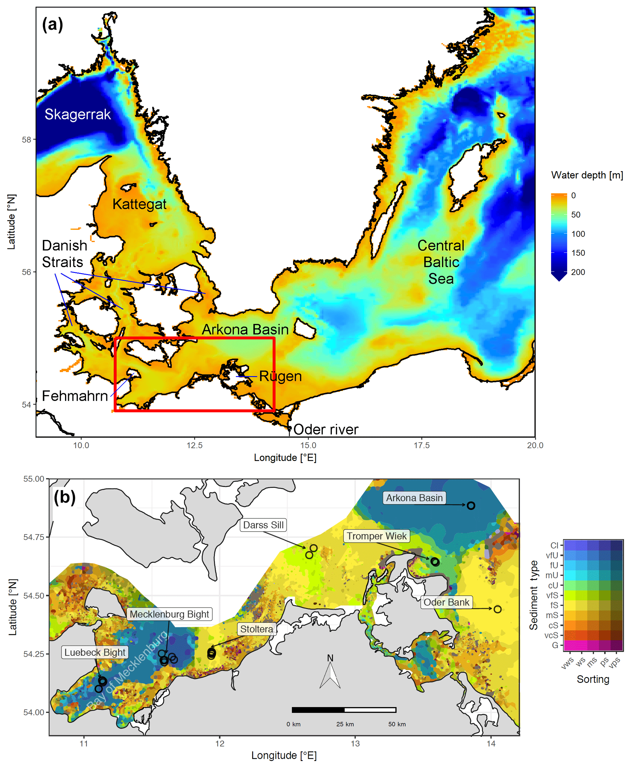
Figure 1(a) Bathymetry of the western Baltic Sea and location of our area of interest. (b) The investigation area of the SECOS project. The map shows granulometry, redrawn from Tauber (2012) and Lipka (2018), and the seven stations considered in this model study. Sediment type: Cl – clay, vfU – very fine silt, fU – fine silt, mU – medium silt, cU – coarse silt, vfS – very fine sand, fS – fine sand, mS – medium sand, cS – coarse sand, vcS – very coarse sand, G – gravel. Sorting: vws – very well sorted, ws – well sorted, ms – moderately sorted, ps – poorly sorted, vps – very poorly sorted.
Understanding and quantifying the scope and scale of such sedimentary services in the German Baltic Sea has been the aim of the SECOS project (The Service of Sediments in German Coastal Seas, 2013–2019). The project contained a strong empirical part, including several interdisciplinary research cruises focused on sediment characterisation. Seven study sites were selected based on different granulometric parameters, each of them representative of a larger area. These were sampled several times in order to capture the effect of seasonality on biogeochemical functioning (see Fig. 1). The sampled stations include three sandy sites at Stoltera (ST), Darss Sill (DS) and Oder Bank (OB), three mud sites at Lübeck Bight (LB), Mecklenburg Bight (MB) and Arkona Basin (AB), and a silty site at Tromper Wiek (TW). The TW site has both an intermediate grain size and an intermediate organic matter content compared to the sandy and muddy sites. In this work, we focus on the development of our coupled one-dimensional benthic–pelagic model system for the German Baltic Sea. We use empirical data obtained from repeated sampling of the SECOS stations to calibrate and validate our early diagenetic model. Further work, discussing the fully coupled three-dimensional application of the model to assessing sedimentary services in the German Baltic Sea, will be described in a forthcoming paper.
1.5 Differences in biogeochemistry between permeable and impermeable sediments
In the study area, different types of sediments dominated by varying grain size fractions are found ranging from sand to mud. This implies differences in the biogeochemical processes associated with organic matter mineralisation and physical processes that are responsible for pore water and elemental transport in the sediment and across the sediment–water interface. Due to its relatively larger grain sizes, sand acts as a permeable substrate, which means that lateral pressure variations may induce the advection of interstitial water. These pressure variations may be caused by waves or by the interaction between horizontal near-bottom currents and ripple formation. In muddy sediments, in contrast, molecular diffusion often controls the transport of dissolved species, which may be superimposed by the bioirrigating activity of macrozoobenthos (Boudreau, 1997; Meysman et al., 2006).
These substantial differences cause differences in the biogeochemical properties of the substrate types. Pore water advection in permeable sediments not only transports solutes but also particulate material. Fresh and labile organic matter (POC and DOC) from the fluff layer can be quickly transported into permeable sediments, the latter in this way acting as a kind of bioreactor. The typically low contents of reactive organics in sand led for a long time to the consideration of sands as “geochemical deserts” (Boudreau et al., 2001). In parallel, the low content of clay minerals and associated organic matter is often accompanied by lower microbial cell numbers when compared to muddy substrates (Böttcher et al., 2000; Llobet-Brossa, 1998). It has, however, been shown that microbial turnover rates in sands may also be high (Al-Raei et al., 2009; Werner et al., 2006). Actually, the supply of fresh organic material may lead to fast microbial degradation rates comparable to those of the organic-rich muddy sediments where more refractory organic material is accumulating at depth. The high mixing rates of pore water in the sands then bring together reactants for secondary reactions like coupled nitrification–denitrification, which makes these areas an effective biological filter, even if pore water concentrations are low compared to impermeable sediments. In our area of investigation, oxygen fluxes and sulfate reduction rates are comparable between sandy and muddy sites, while the organic content differs by an order of magnitude (Lipka et al., 2018a).
1.6 Fluff layer representation
As mentioned earlier, the transport of fluffy layer material from coast to basin areas is an important process in our region of interest. Previous studies with a pelagic ecosystem model (Radtke et al., 2012), which includes fluff layer dynamics, support this experimental finding and highlight the role of this mechanism for the overall nutrient exchange between coasts and basins. For this reason, we explicitly include the fluff layer in our model as a third compartment in addition to the water column and sediment. This approach, which is similar to Lee et al. (2002), is in contrast to most other coupled bentho-pelagic models. We see the explicit representation of fluff layer dynamics as one of the major advantages of our model.
1.7 Article structure
This article is structured as follows. In Sect. 2 we present a description of the model and the processes which are included. In Sect. 3, we summarise which empirical data were used and give a brief explanation of how they were obtained. In Sect. 4, we describe how these data were used to fit the model to the different stations, since the seven stations mentioned before serve as the test case for our model. The model results are shown and discussed in Sect. 5, in which we provide a summary of the scope of model application and its limitations. The paper ends with Sect. 6, in which conclusions and an outlook toward the model's future application within a three-dimensional ecosystem model framework are given.
In this section, we give a description of the combined benthic–pelagic model. We start in Sect. 2.1 with a brief introduction to the two ancestor models it descended from. The model is a purely biogeochemical model, not a physical model, so Sect. 2.2 describes how the physics affecting the biogeochemical processes are prescribed. We then explain the model compartments and state variables in Sect. 2.3. Before giving the full model equations in Sect. 2.5, we first explain the vertical transport processes which occur in these equations in Sect. 2.4.
The core of the model is obviously the biogeochemical processes represented within it. Their description therefore forms the major part of this paper. Biogeochemical processes in the water column are described in Sect. 2.6 and those in the sediment follow in Sect. 2.7. The carbonate system is the same in both compartments and is described separately in Sect. 2.8. Since most of the biogeochemical processes included in our model are already contained in preceding models in exactly the same way, we decided to only give a qualitative description of them in the main text. The quantitative details, including the values of the model constants we used, are presented in a separate, complete description in the Supplement. In contrast, we give a detailed and quantitative description of the “new” processes in the main text, i.e. those that are less common or those that differ from the ancestor models, since we assume that this will be the most interesting part for the majority of readers. The Supplement also contains a table of the model constants and the sensitivities of the model results to changes in the individual parameter values.
The model description is completed by details on numerical aspects given in Sect. 2.9. Finally, in Sect. 2.10, we give a short note on the procedure by which we automatically generate the model code from a formal description of the model processes.
2.1 Ancestor models
The combined benthic–pelagic model is based on two ancestors.
-
The water column part is based on ERGOM, an ecological model developed originally for the Baltic Sea (Neumann, 2000). It has been continuously developed since its first publication, and the latest improvements include introducing refractory dissolved organic nitrogen (Neumann et al., 2015) and transparent exopolymers (Neumann et al., 2017). From the start, ERGOM contained three functional groups of phytoplankton representing large-cell (diatom) and small-cell (flagellate) primary producers as well as diazotroph cyanobacteria and the ability to simulate hypoxic–anoxic conditions.
ERGOM is typically used in a three-dimensional context as a part of marine ecosystem models. With some modifications, it has been applied for different ecosystems such as the North Sea (Maar et al., 2011) and the Benguela upwelling system (Schmidt and Eggert, 2016). It is an intermediate-complexity model for the lower trophic levels up to zooplankton and has been applied for a broad range of scientific questions.
-
The sediment part is based on a model developed for a study on the effect of seasonal hypoxia on sedimentary phosphorus accumulation in the Arkona Sea (Reed et al., 2011). This model is, as many others of its kind, a descendant of the van Cappellen and Wang (1996) model, which focused on the sedimentary iron and manganese cycle and the mineralisation pathways of oxic mineralisation, denitrification and sulfate reduction. An extensive literature survey (combined with model fitting to observations) allowed for the estimation of a large quantity of model constants such as solubility products and half-saturation constants. These were later on inherited by several early diagenetic models, including the one presented in this article. These models solve the diagenetic equations typically applied at a well-defined single site as a one-dimensional set-up.
Like the present one, the model by Reed et al. (2011) is a prognostic model and solves the time-dependent equations rather than making a steady-state assumption.
2.2 Physical parameters used in the model simulations
Since our model is a purely biogeochemical model, it requires a physical environment in which it is embedded. In a final, three-dimensional application, this will be a hydrodynamic host model, and the biogeochemical model described in this communication will be coupled into it. Since we do an intermediate step first and run the model in one-dimensional set-ups, we need to provide physical quantities as model input. The variables which influence the biogeochemical processes in the water column are
-
temperature,
-
salinity,
-
light intensity,
-
bottom shear stress and
-
vertical turbulent diffusivity.
These are prescribed by forcing files1 which need to be provided in order to run the one-dimensional model. We obtain these data from a three-dimensional model simulation of the Baltic Sea ecosystem (Neumann et al., 2017). This simulation was performed using the Modular Ocean Model (MOM) version 5.1 (Griffies, 2018). The model had a horizontal resolution of 3 nm and a vertical resolution of 2 m, covering the entire Baltic Sea. Open boundary conditions were applied in the Skagerrak at the transition to the North Sea. The model was driven by atmospheric forcing data from the coastDat dataset (Weisse et al., 2009), which were extended in time using data from the German Weather Service (Schulz and Schattler, 2014). The ERGOM ecosystem model, as described in the previous section, was implemented in the physical host model, so it produced a hindcast simulation of both the physics and biogeochemistry of the Baltic Sea ecosystem. We extracted model output from the simulated year 2015 at the different locations as input for the 1-D model. Since we run the 1-D model for a longer period, the physical forcing is repeated every year.
2.3 Model compartments and state variables
The one-dimensional model consists of four compartments as shown schematically in Fig. 2:
-
the water column,
-
a fluff layer deposited on the sediment surface,
-
the sedimented solids and
-
the pore water between them.
The water column and sediment are vertically resolved, with the former in layers of 2 m depth such that their number depends on the water depth of the specific site and the latter in 22 layers increasing in depth from 1 mm at the sediment surface to 2 cm at the bottom of the modelled sediment at 22 cm of depth. These specific numbers are not intrinsic to the model but can be changed in the input files2. The current choice of 22 cm for the sediment depth was made according to the availability of pore water data.
Table 1Tracers used in the ERGOM SED v1.0 model.
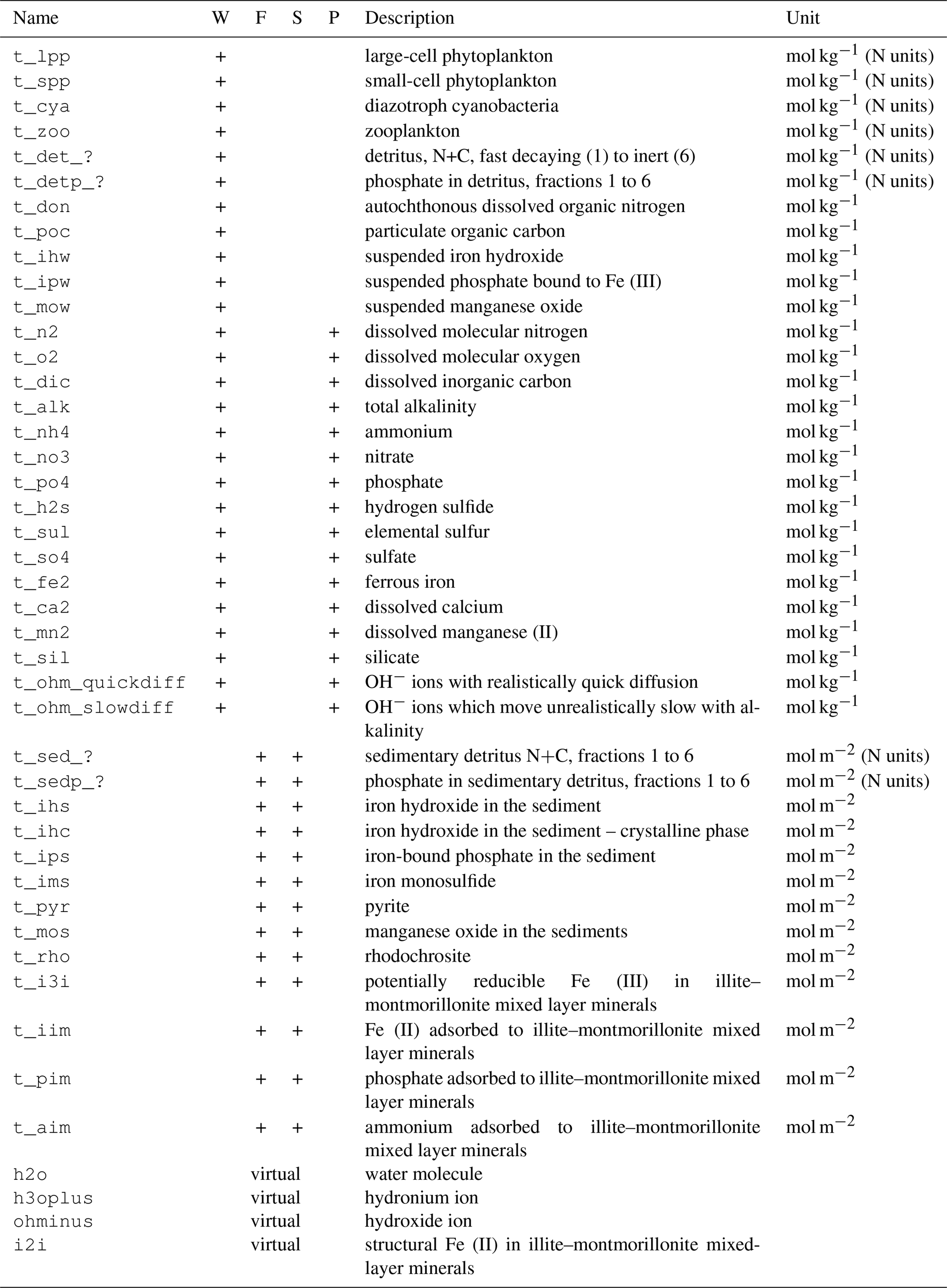
W: water column, F: fluff layer, S: solid sediment, P: pore
water, ?: reactivity classes 1 to 6.
The chosen vertical resolution must be seen as a compromise between speed and accuracy. Especially for the 3-D application, we want to keep the numerical effort of the calculations as small as possible. A comparison to a run with double resolution is shown in Appendix E, and it shows minor deviations among the resolutions.
Sediment porosity is prescribed3 and site specific. As a simplifying assumption, accumulating organic material does not change the porosity. Similarly, the amount of material accumulated in the fluff layer does not change the remaining volume in the bottom water cell.
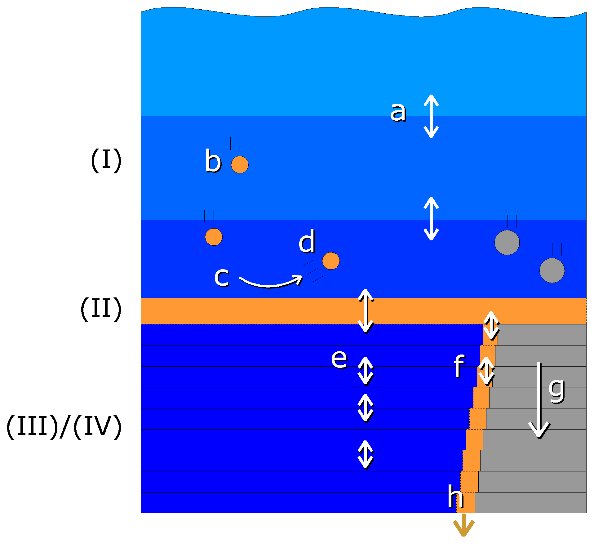
Figure 2Schematic view of the compartments and vertical exchange processes in the model. Compartments: (I) water column, (II) fluff layer, (III) pore water, (IV) solid sediment. Both the water column and sediment consist of several vertically stacked grid cells. Vertical transport processes: a – turbulent mixing, b – particle sinking, c – sedimentation, d – resuspension, e – bioirrigation combined with molecular diffusion, f – bioturbation, g – sediment growth, h – burial. Bioactive solid material is shown in orange, bioinert solid material in grey and water in blue.
The tracers (model state variables) present in each of the compartments are listed in Table 1. All of the tracers have a fixed stoichiometric composition, which is shown in Appendix A. When stoichiometric ratios change, such as during detritus decomposition, more than one tracer is needed. This means we can check mass conservation at the design time of the model by formulating it in a process-based way as outlined in Radtke and Burchard (2015). To check this mass conservation, the chemical reaction equations need to be formulated in a complete way, which is why “virtual tracers” such as water may be included in the process formulation, even if they do not occur as state variables in the model.
Total alkalinity is a parameter describing the buffering capacity of a solution against adding acids; it describes the amount of a strong acid that needs to be added to titrate it to a pH of 4.3. In our model, it is represented as a “combined tracer”, which means that its rate of change depends on its constituents (OH−, H3O+, ) which are actively produced or consumed. The reasoning behind this is explained in Sect. 2.8.
The state variables will not be discussed one by one here, but rather in the section about the biogeochemical processes (Sect. 2.6 and 2.7) where their role in the ecosystem will be explained.
2.4 Transport processes
The processes which transport the tracers vertically are schematically shown in Fig. 2. Their detailed implementation is discussed here.
Horizontal exchange (transport) is neglected in our one-dimensional model. This is obviously an inadequate approximation for the water column processes, as we do not consider basins, but rather single stations, some of which are situated in proximity to river mouths where lateral transport processes have a major impact (Christiansen et al., 2002; Emeis et al., 2002; Schneider et al., 2010). We solve this issue in the future application of the biogeochemical model in a three-dimensional model system (Cahill et al., 2019).
In this model, we are not specifically interested in the water column as such but rather see it as being responsible for delivering the right amount of sedimenting detritus at the right time. To obtain this, we relax the wintertime nutrients in the surface layer to a realistic value. This may be seen as a parameterisation of a lateral exchange process. In addition, transport of fluff layer material away from or towards the modelled location is a lateral process included in the model. The physical processes which are explicitly included in our model are described here.
2.4.1 Turbulent mixing
Vertical exchange due to turbulent mixing in the water column is prescribed externally4 by a turbulent diffusivity. In our case, it is taken from a three-dimensional MOM5 model run (Neumann et al., 2017). In this model set-up, turbulent vertical mixing is estimated by the KPP turbulence scheme (Large et al., 1994), which considers both local mixing and, in the case of unstable stratification, (non-local) convection. We only take into account the local part of the mixing and apply it to all tracers in the water column.
2.4.2 Particle sinking
In our model, suspended particulate matter sinks at a constant rate through the water column. We choose 4.5 m day−1 for detritus, 1 m day−1 for manganese and iron oxides, including the phosphate adsorbed by them, and 0.5 m day−1 for large-cell phytoplankton and particulate organic carbon. In contrast, cyanobacteria are not sinking but, due to their positive buoyancy, they show an upward movement of 0.1 m day−1. In reality, the sinking rate differs among individual particles; the currently chosen average values are a result of fitting the previous ERGOM model with the simplified sediment representation to observations.
2.4.3 Sedimentation and resuspension
Shear stress at the bottom determines whether erosion or sedimentation takes place. We apply the combined shear stress of currents and waves calculated by the same MOM5 model as the turbulent mixing. If this shear stress τ is below a critical value of τc=0.016 N m−2 (Christiansen et al., 2002), the sinking suspended matter accumulates in the fluff layer compartment. If it is exceeded, the fluff layer material is resuspended into the lowest water cell at a constant relative rate rero=6 day−1.
In our model, no material will ever be resuspended from the sediment itself, which starts below the fluff layer. This means that our model is incapable of realistically capturing extreme events like storms or bottom trawling which winnow the upper layers of the sediment, removing organic material, which has a lower sinking velocity, by separating it from the heavier mineral components (Bale and Morris, 1998). It also neglects a washout, which is the removal of organic matter from the sediment pores by advective transport of pore water by strong bottom currents (Rusch et al., 2001). In our model, sediment reworking by currents and waves is not explicitly represented, but rather parameterised together with the bioturbation process. This process allows for a bi-directional exchange of particulate material between the sediment and the fluff layer; see Sect. 2.4.5. The upward component of the transport represents winnowing of sediments (Bale and Morris, 1998).
2.4.4 Bioerosion
In environments with oxic bottom waters, we assume that in addition to waves and currents, macrofaunal animals or demersal fish can resuspend organic material from the fluff layer by active movements (Graf and Rosenberg, 1997). Therefore, under oxic conditions, we assume that rbiores=3 % day−1 of the fluff material is resuspended independently from the shear stress conditions. This number was estimated from the calibration of a three-dimensional Baltic Sea ecosystem model (Neumann and Schernewski, 2008) in which the process proved to be critical for transporting organic matter to the deep basins below a depth of approx. 60 m. In these depths, a resuspension due to wave-induced shear stress is no longer possible.
2.4.5 Bioturbation
Bioturbation describes the movement and mixing of particles inside the sediment caused by the zoobenthos.5 In fact, it is difficult to discriminate what causes the vertical mixing of particles; physical effects like bottom shear may also have the same effect. We therefore include them in our “bioturbation” process.
We consider bioturbation to act as a vertical diffusivity DB,solids(z) on the concentrations of the different solid species in the sediment. This implies that we exclude non-local mixing processes, even if they may be important in nature (Soetaert et al., 1996b), and try to represent them by local mixing. We only take intraphase mixing into account, which means we assume that the porosity Φ(z) remains constant over time.
The diffusivity DB,solids(z) is also applied to describe the transport between the uppermost sediment layer and the fluff, which is caused by benthic organisms. In reality, the fluff layer may strongly differ in its compaction (porosity) depending on the turbulence conditions. However, we assume it to be perfectly compacted (ϕ=0) to be able to apply the above equation to describe the exchange process and therefore assume a thickness of 3 mm. This is not a physical assumption but rather a numerical trick which we use to transport the fluff material into the sediments. In reality, the fluff layer may be up to a few centimetres thick, and the incorporation of organic matter is done by macrofaunal activities (van de Bund et al., 2001).
The value 3 mm describes a volume estimate of SPM (suspended particulate matter) taken from this region: typical SPM concentrations in the lowermost 40 cm of the water column are about 8 mg L−1 higher compared to the value 5 m above the sea floor (Christiansen et al., 2002). As the density of these particles is just slightly higher than that of the surrounding water, we can estimate their volume at approximately 3 L m−2, which gives 3 mm of height if perfectly compacted. We see this explicit treatment of the fluff layer as a major advantage compared to the deposition of sinking particles directly into the surface sediments. We regard it as essential for the application of the model in a three-dimensional setting.
The vertical structure of bioturbation intensity, DB,solids(z), is parameterised vertically as follows.
In the uppermost part of the sediment, we assume a constant bioturbation rate. Below that, it decays exponentially with depth until it reaches a maximum depth, which may be below the bottom of our model. So, we externally prescribe (a) the maximum mixing intensity6 and (b) three length scales describing the vertical structure of bioturbation7, which are the depth down to which the maximum mixing rate is applied (zfull), the length scale of the exponential decay of the mixing rate below this depth (zdecay) and the maximum depth of mixing (zmax).
The present formulation of the model has no explicit dependence of bioturbation depth on the availability of oxidants, i.e. bioturbation will take place in oxic as well as in sulfidic environments; adding this dependence should be essential if the model is applied to sulfidic areas.
2.4.6 Bioirrigation
Bioirrigation describes the mixing of solutes within the pore water and the exchange with the bottom water. We describe it as a mixing intensity DB,liquids(z). The vertical profile of bioirrigation intensity is assumed identical to that of bioturbation. The maximum bioirrigation rate is assumed constant in time and prescribed externally8.
2.4.7 Molecular diffusion
Molecular diffusion in the sediment can be described by the equation
(Boudreau, 1997). Here, D0 describes the molecular diffusivity in a particle-free solution, which is effectively reduced by the effect of hydrodynamic tortuosity θ. This describes the effect that the solutes need to travel a longer path as the direct way may be obstructed by solid particles. It is estimated from porosity by (Boudreau, 1997).
A diffusive exchange between the pore water and the overlying bottom water is controlled by the thickness of a diffusive boundary layer. While in reality this relates to the viscous sublayer thickness and is therefore inversely related to the velocity of the bottom water (Boudreau, 1997), for simplicity we assume a constant diffusive boundary layer thickness of 3 mm.
In reality, the diffusive boundary layer thickness is on the order of 1 mm at low-bottom-shear situations and becomes even shallower if the bottom shear increases (Gundersen and Jorgensen, 1990). We choose a larger value because we need to account for the transport through the fluff layer as well. A future model version might include a dependence of this parameter on the bottom shear stress.
Molecular diffusivities for the different solute species are calculated from
water viscosity following Boudreau (1997). The water viscosity is
determined from salinity and temperature (assumed to be identical to that in
the bottom water cell). A problem occurs with the combined tracers DIC and
total alkalinity, as they do not represent a specific ion but rather a set of
different species with different molecular diffusivities. For simplicity, we
approximate DIC diffusivity to be that of the ion, the most common
one at the pH values we expect. For total alkalinity, we take a two-step
approach: in the first step, we also take the diffusivity of the
ion. But this is an underestimate, especially for the OH− ions, which
increase in concentration as the solution becomes alkaline. To take
their higher diffusivity into account, we introduce two additional tracers,
t_ohm_slowdiff and t_ohm_quickdiff. Before the
molecular diffusion is applied during a model time step, they are both set
equal to the OH− concentrations. During the diffusion time step, the
former diffuses with the reduced diffusion rate, the latter with
the OH− diffusivity. So afterwards, total alkalinity is corrected by
adding the difference of the two,
t_ohm_quickdiff-t_ohm_slowdiff. This results in a
smoothed alkalinity profile.
2.4.8 Sediment accumulation
In nature, sediments grow upwards as new particulate matter is deposited onto them. In our model, this process is taken into account, but represented as the downward advection of material in the sediment. So, our coordinate system moves upward with the sediment surface. We assume that the sediment growth is supplied by terrigenous, bioinert material and prescribe9 a growth rate from the literature for the mud stations only (Table 7). We do not assume sediment growth for the sand and silt stations.
We use a simple Euler-forward advection to move the material from each grid cell into the cell below. Material leaving the model through the lower boundary is lost. Except for organic carbon, we assume that a part of it is mineralised, as will be explained in Sect. 2.7.1. In the top cell, new organic material from the fluff layer enters by sediment growth.
2.4.9 Parameterisation of lateral transport
The Baltic Sea sediments can be classified as accumulation, transport and erosion bottoms (Jonsson et al., 1990). The lateral transport of matter is characterised by the advection of fluff layer material from the transport and erosion bottoms in the shallower areas to the accumulation bottoms in the deep basins (Christiansen et al., 2002). As this process is not represented in our 1-D model set-ups, we need to parameterise it.
For the sandy and silty sediments, we assume transport away from the site. This is described by a constant removal rate for all material deposited in the fluff layer. For the mud stations, we assume transport of organic material towards the site. This is described by a constant input of detritus. Our model contains six detritus classes which degrade at different rates, as will be explained later in Sect. 2.6.4. We assume that the quickest-degradable part of the detritus is already mineralised in the shallow coastal areas before its lateral migration to the mud stations and therefore exclude the first two classes from this artificial input.
In the 3-D version of the model, these processes are no longer required, as the material is dynamically removed from the shallow sites and transported to deeper ones by advection.
2.5 Model equations
2.5.1 Equations of motion
In this subsection, we will describe the equations of motion solved by the model. The equations in the water column can be derived from the assumption that the vertical (upward) flux of a tracer can be described by an advective and a diffusive flux, which follows Fick's law:
where cwat(z,t) denotes the tracer concentration and Dwat is the turbulent diffusivity given as external forcing10. For particulate matter, the constant w describes its vertical velocity relative to the water, which is negative if the particles are sinking. For dissolved tracers, w is set to zero. We further assume that the water itself does not move vertically. In this case, conservation of mass yields an advection–diffusion equation:
where describes the biogeochemical sources minus sinks of the considered state variable.
The equations in the sediment are different because we need to take porosity into account and treat dissolved tracers (in the pore water) and solid tracers differently. For the pore water tracers, the upward flux is given by
where ϕ(z) is the porosity of the sediment (the ratio between pore water volume and total volume), which we assume as constant in time. The concentration cpw(z,t) relates to the pore water volume only. The effective diffusivity Dpw is the sum of two contributions, the effective molecular diffusivity and the effective (bio)irrigation diffusivity DB,liquids(z). The advection–diffusion equation is then given by
which is a well-known early diagenetic equation (Boudreau, 1997). For the solid-state tracers, their concentration csed(z,t) relates to the volume of the solids only, and the flux is given by
where w(z) is the velocity for virtual vertical downward transport. It results from sediment growth due to the deposition of particulate material, but as we keep the sediment–water interface at a constant position in our model, we need to describe the increasing depth in which we find individual sediment particles as downward advection. Volume conservation of the particulate material requires that we write w(z) as
such that the vertical velocity gets smaller in depths at which the sediment is more compacted, and w0 describes a theoretical velocity which would occur at perfect compaction (ϕ=0)11. The advection–diffusion equation then reads
Practically, we do not store the concentration csed(z,t) (mol m−3) as a state variable but rather the quantity of the tracer per area in a specific layer, Csed(k,t) (mol m−2), where k is a vertical index. The transformation is straightforward:
For particulate tracers, we also consider storage in the fluff layer, Cfluff(t), which is measured in mol m−2. The equation for Cfluff(t) is derived in the following subsection.
2.5.2 Boundary conditions
Boundary conditions are required for the partial differential equations given above. We give two boundary conditions for the water column concentrations: one at the sea surface, zsurf, and one at the sediment–water interface, z0. We also give two boundary conditions for the sediment concentrations: one at the sediment–water interface, z0, and one at the lower model boundary, zbot. We start describing the boundary conditions from bottom to top for the dissolved tracers and then continue describing them from top to bottom for the particulate and solid-phase state variables.
The pore water tracers have a zero-flux boundary condition at the bottom of the model:
An exception to the zero-flux boundary is the parameterisation of sulfide production in the deep, which will be discussed later.
At the sediment–water interface, we assume that the dissolved tracers are exchanged between pore water and the water column via a diffusive boundary layer of a depth Δzbbl. So, our upper boundary condition for the pore water tracers is given by
This flux can be directed into or out of the sediment, depending on where the concentration is larger.
To satisfy mass conservation, the vertical flux applied as the lower boundary condition for the dissolved species concentrations in the water column depends on the upward flux from the sediment:
The additional term represents the sources minus sinks of the dissolved state variable, which are caused by biogeochemical transformations of the fluff layer material. At the sea surface, we apply a zero-flux condition, both for dissolved and particulate state variables:
An exception is only made for tracers which are modified by gas exchange with the atmosphere, e.g. oxygen.
Now the boundary conditions for the particulate state variables are different. The reason is that the water column and the sediment do not directly interact, but we consider the fluff layer as an intermediate layer between the two. Particulate material which sinks to the bottom is deposited in the fluff layer, from which it is incorporated into the sediments.
At the bottom of the water column, there can be two possible situations.
-
If the bottom shear stress is lower than the critical shear stress, we assume a deposition of particulate material. This sinking material (w<0) vanishes from the water column because of sedimentation. It appears in the fluff layer.
-
If the bottom shear stress exceeds the critical shear stress, particulate material from the fluff layer is eroded and enters the water column.
In both cases, we additionally consider the bioresuspension process which was described above in Sect. 2.4.4. We can therefore formulate the boundary condition for particulate material as
The fluff interacts with the surface sediment layer in two ways. Firstly, sediment growth means an incorporation of fluff layer material into the surface sediments. Secondly, bioturbation, which is considered diffusion–analogue mixing, leads to an exchange of particulate material between the fluff layer and surface sediment. So, the boundary condition for solids at the sediment surface is given by
Here, Δzfluff represents a virtual thickness of the fluff layer assuming it was perfectly compacted; see the discussion in Sect. 2.4.5. In this way, the benthofaunal processes of incorporating fluff layer material into the surface sediments can be simply described as a diffusion–analogue flux of particulates. The opposite processes which cause removal of fine-grained material from the sediments, winnowing or washout, can be described in the same way as a diffusion process, in this case upward. This occurs in the model, especially when the fluff layer material is resuspended during periods of high bottom shear and the concentration Cfluff(t) is correspondingly low.
The concentration change in the fluff layer is then defined by mass conservation and is simply given by
for all particulate state variables. Here, describes the sources minus sinks term from the biogeochemical transformations of the considered state variable.
Table 2Reaction network table for the processes in the water column. See Table A1 for the composition of state variables. Processes marked with * also take place in the pore water.

Finally, the burial of particulate material at the lower model boundary can be described by the following boundary condition:
So, we assume the particulate material to be buried forever when it leaves the model domain. An exception, as mentioned before, is the parameterisation of deep sulfide formation, which is described in Sect. 2.7.
2.6 Biogeochemical processes in the water column
In this section, we describe the biogeochemical processes acting in the water column. These are mostly identical to previously published ERGOM versions (Neumann and Schernewski, 2008; Neumann et al., 2015), which contained a more simple, vertically integrated sediment model. As in the previous section, we provide a quantitative description including the model constants in the Supplement.
A reaction network table giving the reaction equations, including their stoichiometric coefficients, is given in Table 2.
2.6.1 Primary production and phytoplankton growth
There are three classes of phytoplankton in the model, representing large-cell and small-cell microalgae as well as diazotroph cyanobacteria. Their growth is determined by a class-specific maximum growth rate, but contains two limiting factors for nutrients and light. The light limitation is a saturation function with optimal growth at a class-specific optimum level or at 50 % of the surface radiation. The shortwave light flux at the surface is taken from a dynamically downscaled ERA40 atmospheric forcing (Uppala et al., 2005) using the regional Rossby Centre Atmosphere model (RCA). Nutrient limitation is a quadratic Michaelis–Menten term for DIN (nitrate + ammonium) or phosphate, depending on which one is limiting, based on Redfield stoichiometry. Diazotroph cyanobacteria are only limited by phosphate and not by DIN, but they are only allowed to grow in a specific salinity range. Cyanobacteria and small-cell algae also require a minimum temperature to grow (Andersson et al., 1994; Wasmund, 1997).
However, according to Engel (2002), although nutrients are limiting an enhanced polysaccharide exudation could be the result of a cellular carbon overflow whenever nutrient acquisition limits biomass production but not photosynthesis. These transparent exopolymers are included in our model, and they are assumed to have a constant sinking velocity.
2.6.2 Phytoplankton respiration and mortality
We assume a constant respiration of phytoplankton which is proportional to its biomass. As the model maintains the Redfield ratio, the degradation of biomass (catabolism) goes along with the excretion of ammonium and phosphate. This simplified description of phytoplankton growth does not describe day–night metabolism or temperature dependence. A small fraction of the nitrogen is released as dissolved organic nitrogen (DON). In the model, this represents the DON fraction which is less utilisable by phytoplankton, while the fraction with high bioavailability is considered to be part of the ammonium state variable.
Due to simplification, in our model phytoplankton experiences a constant background mortality, although we know this is far away from reality in which it is species specific and depends on abiotic (e.g. nutrient, light, etc.) and biotic conditions. An additional mortality is generated by the grazing of zooplankton as described next.
2.6.3 Zooplankton processes
Zooplankton is only represented as one bulk state variable. It grows by assimilating any type of phytoplankton; however, it has a smaller food preference for the cyanobacteria class compared to the other classes. The uptake becomes limited by a Michaelis–Menten function if the zooplankton's food approaches a saturation concentration. Feeding can only take place in oxic waters and is temperature dependent. It shows a maximum at an optimum temperature and a double-exponential decrease when this temperature is exceeded.
Both zooplankton respiration and mortality represent a closure term for the model. They are meant to include the respiration and mortality of the higher trophic levels (fish) which feed on zooplankton, and therefore we use a quadratic closure. Mortality is additionally enhanced under anoxic conditions, which do not occur in our study area.
2.6.4 Mineralisation processes
The description of detritus12 differs from the previous ERGOM versions. We have split the detritus into six classes, depending on its degradability. This degradability is described as a decay rate constant, which ranges from 0.065 day−1 for the first class to day−1 for the fifth class, while the last one is assumed to be completely bioinert. This type of model is known as a “multi-G model” (Westrich and Berner, 1984).
Details on the specific choice of the classes are given in Appendix B.
The mineralisation is, however, temperature dependent by a Q10 rule (Sawicka et al., 2012; Thamdrup et al., 1998), as it is realised by microbial processes; the values given above are valid at 0 ∘C. The 0 ∘C choice is somewhat arbitrary. Actually, the model is not very sensitive to this choice, as an enhanced baseline temperature, meaning a lower decomposition rate of each class, would be compensated for by a shift in the class composition, leaving higher concentrations of quickly degradable detritus classes, which overall means a very similar total decomposition rate; see Appendix B.
When organic detritus is created by plankton mortality, it is partitioned into the different classes in a constant ratio. This ratio was determined from a fit of the multi-G model to an empirical relation between detritus age and its relative decay rate, which was proposed by Middelburg (1989). The fraction of non-decaying detritus was estimated from empirically determined carbon burial rates in the Baltic Sea (Leipe et al., 2011).
The chemical composition of detritus is, in contrast to phytoplankton and zooplankton, not determined by the Redfield ratio. It is enriched in carbon and phosphorus by 50 % such that it has a C : N : P ratio of 159 : 16 : 1.5. This resembles detritus compositions as they were determined in sediment traps and by investigating fluffy layer material in the Baltic Sea (Emeis et al., 2000, 2002; Heiskanen and Leppänen, 1995; Struck et al., 2004).
In the water column, detritus can be mineralised by three different oxidants: oxygen, nitrate and sulfate. They are utilised in this order; if the preferential oxidant's concentration declines, the specific pathway is reduced by a Michaelis–Menten limiter and the next pathway takes over such that the total mineralisation is held constant. In all pathways, DIC, ammonium and phosphate are released. Nitrate reduction also produces molecular nitrogen (heterotrophic denitrification), while sulfate reduction generates hydrogen sulfide.
Mineralisation of particulate organic carbon in transparent exopolymers takes place via the same pathways, but only releases DIC. DON is also mineralised after some time and decays to ammonium (which may represent the transformation to bioavailable DON compounds).
2.6.5 Reoxidation of reduced substances
In the presence of oxygen, ammonium is nitrified to nitrate (Guisasola et al., 2005). The intermediate step, the formation of nitrite, is omitted in the model. Hydrogen sulfide can be reoxidised by oxygen or by nitrate (chemolithoautotrophic denitrification) (Bruckner et al., 2013). This takes place as a two-step process via the formation of elemental sulfur (Jørgensen, 2006). All reoxidation processes exponentially increase their rates with temperature.
In the sediments, we additionally assume that Fe2+ can be produced as a reduced substance. If it is released from the sediments and enters the water column, it can be reoxidised by oxygen, creating suspended iron oxyhydroxides.
2.6.6 Adsorption and desorption reactions
Dissolved phosphate can be adsorbed to iron oxyhydroxide particles suspended in the water column. In the same way, phosphate adsorbed to iron oxyhydroxide particles can be released if the ambient concentration of phosphate is low. The process is identical to the one in the sediments and is discussed in Sect. 2.7.5 in detail.
2.7 Biogeochemical processes in the fluff layer, sediment and pore water
In this section, we qualitatively describe the sedimentary biogeochemical processes contained in the model. For a quantitative description including the model constants, we refer to the Supplement. Figure 3 gives a schematic overview of the processes considered in the sediment model. As with every model, the chosen set of biogeochemical processes and variables does not aim at completeness in its representation of reality, but rather at the strongest possible simplification which still retains the required complexity to describe the processes we are interested in. For this reason, we do not, for example, consider methane formation explicitly.
Table 3Reaction network table for the primary redox reactions in the sediment and the fluff layer. See Table A1 for the composition of state variables.
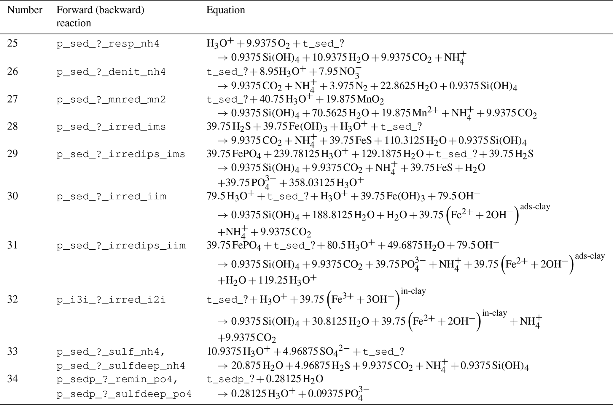
Table 4Reaction network table for the secondary redox reactions in the sediment and in the fluff layer.
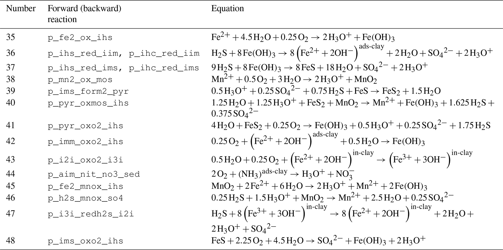
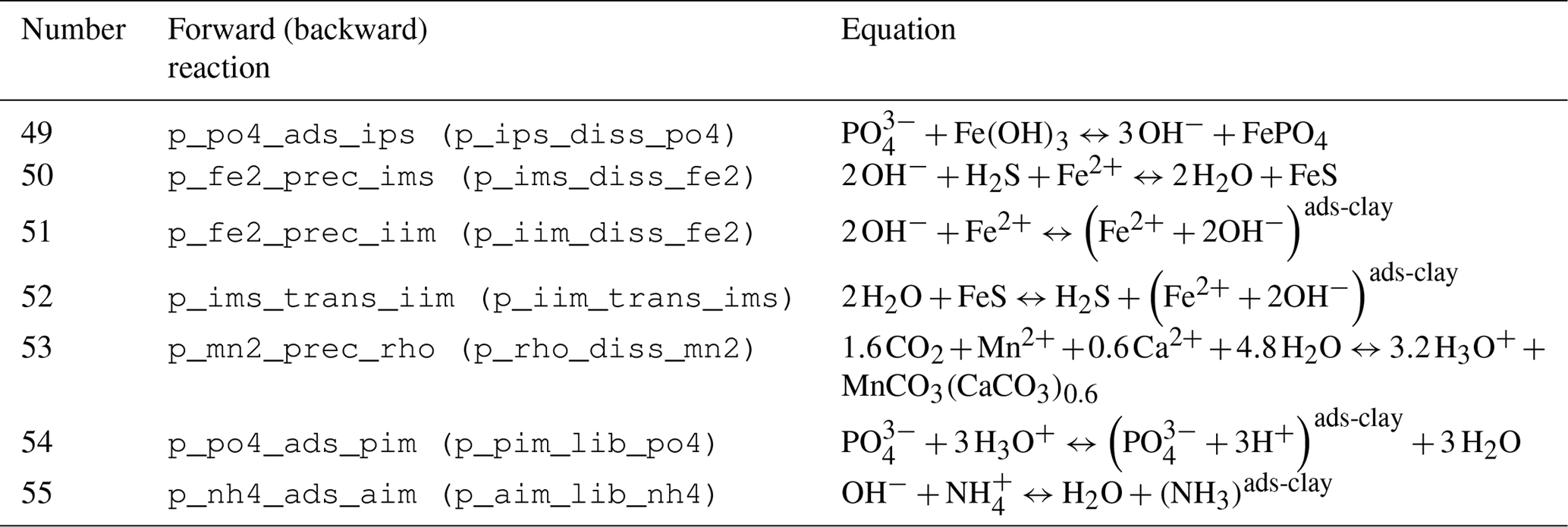
Table 5Reaction network table for adsorption–desorption and precipitation–dissolution processes in the sediment and in the fluff layer.
The stoichiometry of the processes included in the model is shown in three reaction network tables.
-
Primary redox reactions are given in Table 3.
-
Secondary redox reactions are given in Table 4.
-
Adsorption–desorption and precipitation–dissolution reactions are given in Table 5.
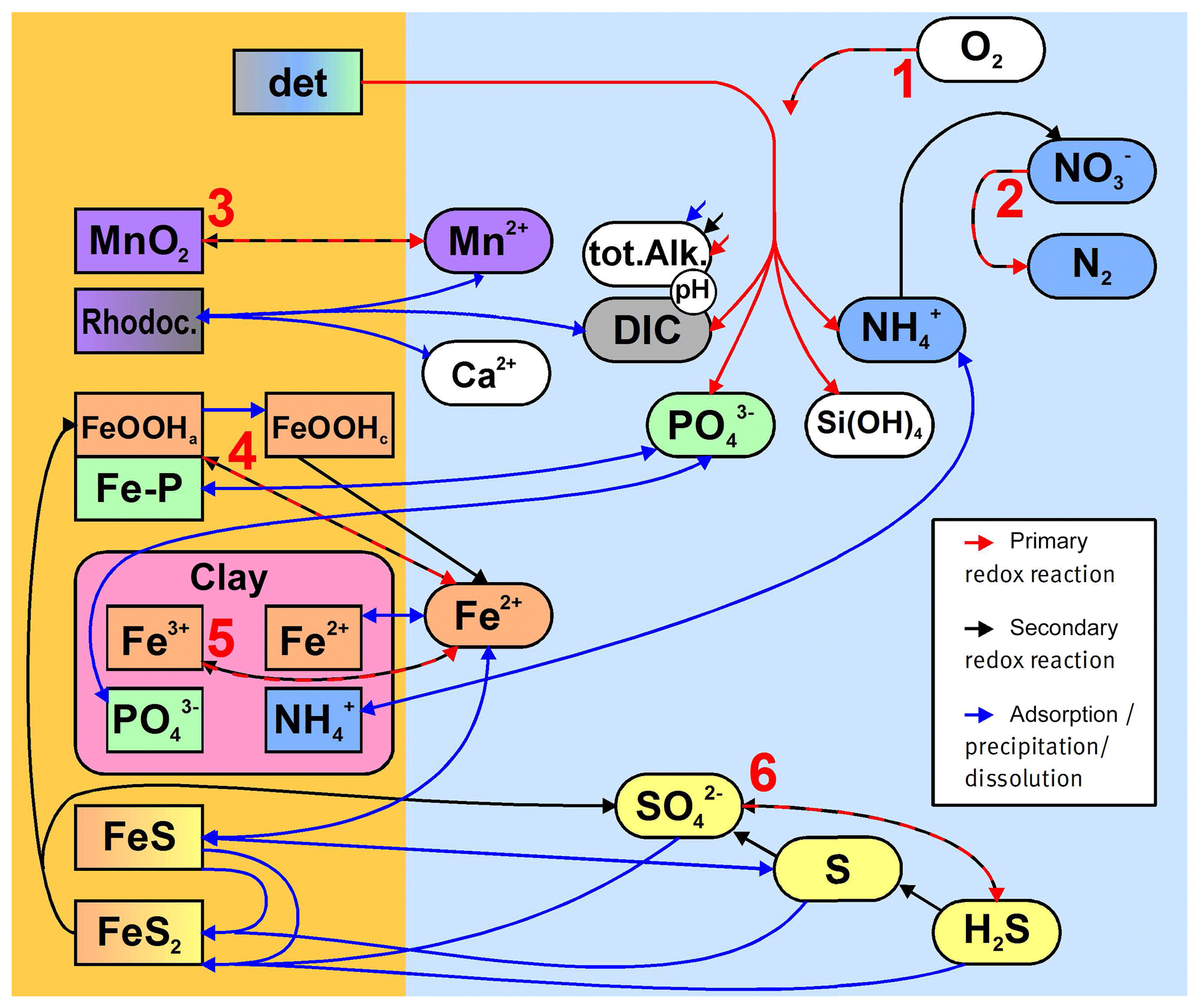
Figure 3Simplified sketch of state variables and processes in the sediment model. Boxes to the left and right indicate sediment and pore water state variables, respectively. pH is not a state variable but calculated from DIC and total alkalinity. Red arrows show primary redox processes driven by the oxidation of organic carbon. The red numbers indicate the order in which the oxidants are utilised. Black arrows show secondary redox reactions, which means reoxidation of reduced substances. Blue arrows show adsorption–desorption or precipitation–dissolution reactions, which may depend on pH. Abbreviations: det – detritus, Rhodoc. – rhodochrosite, tot.Alk. – total alkalinity, DIC – dissolved inorganic carbon.
2.7.1 Mineralisation in general
The mineralisation of detritus is the dominant biogeochemical process in the sediments, as the oxidation of the carbon therein is the major supply of chemical energy for microbes.
As in the water column, oxidants are utilised in a specific order, and a smooth transition to the next mineralisation pathway occurs when the preferred one gets exhausted. However, the number of possible oxidants is increased in the sediment, as here solid components may also act as electron acceptors. The order in which they are utilised is (Boudreau, 1997)
-
oxygen,
-
nitrate,
-
manganese oxide,
-
iron oxyhydroxide,
-
Fe (III) contained in clay minerals and
-
sulfate.
After sulfate is exhausted, typically the formation of methane would start. This process is omitted in the current model, as we designed our model for the top 22 cm of the south-western part of the Baltic Sea, where we do not expect sulfate to be limiting. This depth restriction is based on the limited length of the sediment cores taken in the empirical part of our research project. We do, however, describe the process implicitly, since we assume that a part of the organic carbon which leaves the model domain through the lower boundary will be transformed to methane, which as it diffuses upward will be oxidised by sulfate and generate H2S. Therefore, we parameterise this process by a conversion from sulfate to hydrogen sulfide at the lower boundary.
As in the water column, we distinguish six different classes of detritus with different basic mineralisation rates.
Details on the specific choice of the classes are given in Appendix B.
These rates are only controlled by temperature, not by the specific oxidant which is available. There is an ongoing controversy as to what determines the rate of sedimentary carbon decay and whether it is the oxidant (and therefore the accessible energy per mole of carbon) or the degradability of the detrital carbon itself (Arndt et al., 2013; Kristensen et al., 1995). In leaving out the explicit dependence of the oxidant, we do not favour the latter theory; we chose to adopt the decay rates proposed by Middelburg (1989), which may implicitly take the effect of the oxidant into account13.
Sedimentary organic phosphorus (OP) may degrade faster than the corresponding
nitrate and carbon, an effect known as preferential P mineralisation
(Ingall and Jahnke, 1997). We include this by introducing additional state variables
t_detp_n for each class n of detritus, describing the OP
concentration, as well as a constant factor pref_remin_p, which
describes a redox-dependent ratio between the mineralisation speeds of OP and
organic carbon and nitrogen. This factor is set equal to 1 under oxic
conditions and greater than 1 under anoxic conditions (Jilbert et al., 2011).
This approach follows Reed et al. (2011).
2.7.2 Specific mineralisation processes
Here, we describe the implementation of the primary redox reactions, indicated by the red numbers in Fig. 3.
Oxic mineralisation and heterotrophic denitrification are formulated in the same way as in the water column; see Sect. 2.6.4.
The next pathway is the reduction of Mn (IV) to Mn (II), which produces dissolved manganese.
The reduction of iron oxyhydroxides should produce dissolved Fe (II). This, however, may precipitate very quickly, especially where hydrogen sulfide is present. So for numerical reasons, we combine these reactions, and the reduced Fe (III) is directly converted into iron monosulfide or considered as adsorbed by clay minerals, as we describe below in Sect. 2.7.3.
Some clay minerals, especially sheet silicates which are abundant in the German part of the Baltic Sea (Belmans et al., 1993), contain structural iron which is available for redox reactions (Jaisi et al., 2007). We prescribe a station-specific content of these minerals given in Table 7 and assume that they contain a small amount (0.1 mass-%) of reducible iron; this is because a particle analysis of sheet silicates from the area of interest (Leipe, unpublished data) showed slightly lower iron contents in the sulfidic zone compared to the surface area.
The primary redox reaction follows process 32 in Table 3; we describe it in detail since it is a new process added to our model. Mineralisation of organic carbon under the reduction of structural iron in sheet silicates takes place at a rate of
where t_sed_k is the amount of detritus per area in a specific
sediment layer, rk is a basic reactivity for this class (see
Appendix B), τ=0.15 K−1 is a temperature
sensitivity constant for the mineralisation and T is the temperature in
∘C. The limitation functions l? are of Ivlev type, e.g.
they have a value close to 1 at high concentrations of the corresponding oxidant and become zero if this oxidant is exhausted. Here, O2,min denotes a threshold concentration at which the limitation occurs, but the Ivlev function generates a soft transition between the different oxidation pathways, so they can occur simultaneously. The product of the last five factors in Eq. (19) means this process will run at a substantial rate only if
-
oxygen concentration is low,
-
nitrate concentration is low,
-
manganese oxides in the sediment are depleted and
-
iron oxyhydroxides in the sediment are depleted, but
-
reducible structural Fe (III) in the clay minerals is still abundant.
Sulfate reduction produces hydrogen sulfide. As discussed above, it represents the terminal mineralisation process in our model. This process, described by processes 33 and 34 in Table 3, follows the formulation by Reed et al. (2011) in our model. Organic material leaving the lower boundary of our model because of sediment growth will also be mineralised by this process. We assume that a fraction of the buried material will be mineralised by either sulfate reduction or methanogenesis, the rest being buried. For the methane produced, we assume that it will not enter the model domain but rather be oxidised by sulfate, producing H2S below the model domain. We assume for simplicity that all these reactions happen instantaneously, which results in the same net reaction as the sulfate reduction.
2.7.3 Precipitation and dissolution reactions
Solids can precipitate from a solution when it becomes supersaturated. This happens in an aqueous solution when the actual ion activity product exceeds the respective solubility product and a critical degree of supersaturation is reached (Böttcher and Dietzel, 2010; Sunagawa, 1994).
Diagenetic models often simplify the calculation by multiplying the concentrations rather than the activities (van Cappellen and Wang, 1996). The resulting product is then proportional to the actual solubility product as long as the ionic strength of the solution does not change. As the ionic strength of seawater is almost completely defined by its salinity (Millero and Leung, 1976), this assumption is well justified for most marine environments. The Baltic Sea, however, is a brackish sea with strong spatial and temporal changes in bottom salinity, especially in the western part (Leppäranta and Myrberg, 2009). For this reason, we take the activity coefficients, which transform concentrations to activities, into account. This is done by using the Davies equation (Davies, 1938), which determines the individual activity coefficient ai as (Stumm and Morgan, 2012)
where I is the ionic strength expressed in mol L−1, zi is the ion charge and A is the Davies parameter calculated after Kalka (2018):
Here, ϵ is the dielectric constant of water calculated after Gadani et al. (2012)14, and TK is the temperature in K.
Ca–rhodochrosite precipitates at elevated concentrations of manganese and carbonate. Its solubility product is composition dependent, as the Ca : Mn ratio varies (Böttcher, 1997; Böttcher and Dietzel, 2010). For Baltic Sea muds in which ratios around 0.6 occur, an effective solubility product (including the effect of oversaturation) of 10−9.5 to 10−9 M2 can be deduced from Jakobsen and Postma (1989). In our model, the reaction follows process 53 in Table 5. 10 % of the dissolved manganese will precipitate per day if the solution is undersaturated. Saturation is calculated by the formula (Jakobsen and Postma, 1989)
where is the concentration of carbonate ions, which depends on DIC concentration and pH; see the description of the carbon cycle in Sect. 2.8. The term a2 is the activity coefficient for ions with a charge of 2; see Eq. (21). The term in the denominator is the solubility product for rhodochrosite (Jakobsen and Postma, 1989).
If the solution becomes undersaturated, rhodochrosite will be dissolved again. Then, process 53 is reversed, and a fixed amount of 10−6 mol kg−1 day−1 of manganese (II) is released until saturation is reached.
Iron monosulfide precipitates on contact with dissolved Fe (II) and sulfide, depending on pH, with a solubility product taken from Morse et al. (1987). But, as stated in Sect. 2.7.2, we assume for numerical reasons that this process takes place directly after Fe (III) reduction. The solubility product is then used in an inverse way to determine the equilibrium concentration of dissolved Fe (II) at the current pH, sulfide concentration and salinity:
where ai represents the Davies activity coefficients (see Eq. 21), and 10−2.95 mol L−1 is the solubility product for iron monosulfide (Morse et al., 1987; Theberge and Iii, 1997).
We then assume a precipitation or dissolution of iron monosulfide, which relaxes the present concentration of Fe (II) against this equilibrium. This is in agreement with a pore water chemistry model for the central Baltic Sea (Kulik et al., 2000), which states that dissolved iron concentrations in the pore water are buffered by iron sulfides (mackinawite and greigite). The dissolution of iron monosulfide also takes place if clay minerals in the same grid cell are capable of adsorbing additional Fe (II). This process is described in Sect. 2.7.5.
As a simplification, we neglect the change in porosity which would be caused by precipitation (or dissolution) of any solids.
2.7.4 Pyrite formation
Pyrite (FeS2) is a crystalline compound formed in early diagenesis (Rickard and Luther, 2007). Its formation from iron monosulfide is included in most early diagenetic models. This process is not a simple precipitation process, but rather a redox process. While both sulfide and iron monosulfide contain sulfur of oxidation state −2, the redox state of S in pyrite is −1. This implies that an electron acceptor is required to create pyrite. A generally accepted mechanism for pyrite creation is the use of zero-valent sulfur from polysulfides; this may be created by the oxidation of sulfate with Fe (III). However, this process alone cannot explain the high degrees of pyritisation in Baltic deep sediments (Boesen and Postma, 1988).
An additional pathway which does not rely on elemental sulfur, but instead reduces hydrogen sulfide to hydrogen gas, has been proposed by Drobner et al. (1990), Rickard and Luther (1997), and Rickard (1997). Similar to how it was done in early diagenetic models (Wijsman et al., 2002), we include this pathway and therefore assume that whenever iron monosulfide and H2S are present, pyrite is formed from them. The generated H2 will be consumed by sulfate-reducing bacteria (Stephenson and Stickland, 1931), so in the net reaction, sulfate acts as the electron acceptor.
In our model, the reaction therefore follows process 39 in Table 4. The speed of the transformation process is determined by
where 𝚝_𝚒𝚖𝚜 is the concentration of iron monosulfide, 𝚝_𝚑𝟸𝚜 is the concentration of hydrogen sulfide and kpyr is a kinetic constant for conversion of iron monosulfide to pyrite. Its value of 8.9 kg mol−1 day−1 was adopted from Wijsman et al. (2002) and Rickard and Luther (1997), which use 8.9 L mol−1 day−1.
2.7.5 Adsorption balances
Adsorption in our model takes place on the surfaces of two particle types: iron oxyhydroxides and clay minerals. Adsorption on silicate particles is not explicitly represented in the model, but parameterised by a reduction of the effective diffusivity of phosphate and ammonium, following Boudreau (1997).
Iron oxyhydroxides adsorb dissolved phosphate. This is a well-known process responsible for the sedimentary retention of phosphate derived from mineralisation processes (Sundby et al., 1992). As both phosphate and hydroxide ions can occupy the adsorption sites at the surface, adsorption is less efficient in alkaline environments. In our model, we use a formula from Lijklema (1980) which describes the adsorbed P : Fe ratio at a given phosphate concentration and pH.
Here, DIP gives the dissolved phosphate concentration. But we use it inversely. We calculate an equilibrium concentration for dissolved phosphate at the current P : Fe ratio and pH.
If the current concentration of dissolved phosphate is above this equilibrium
concentration, adsorption takes place and PO4 in the pore water is
decreased. If it is below the equilibrium concentration, desorption takes
place. The maximum function is added to treat situations when both pH and
the amount of adsorbed phosphate get so low that the formula by
Lijklema (1980) gives no real solution for DIP. In this case, we assume
that all currently dissolved phosphate will become adsorbed. The model
processes p_po4_ads_ips and p_ips_diss_po4 will
change the phosphate concentration in the pore water by
where k_ips_dissolution = 0.1 day−1 is a reaction rate
constant we assume. We chose this probably unrealistically low value for
reasons of numerical stability.
Following Reed et al. (2011), we define two classes of iron oxyhydroxides. The first one is fresh, amorphous and adsorbs phosphate. The second one is a more crystalline phase, for which we assume no adsorption. The first phase is transformed to the second one with a constant rate in time, implying continuous phosphate release.
Clay minerals, due to their large surface area, can also adsorb pore water species. We allow for an adsorption of phosphate, ammonium and Fe (II). For simplicity, we assume that the ratio of adsorbed species to clay mass is proportional to the pore water concentration until a saturation threshold is exceeded. For Fe (II), this proportionality constant is derived from Jaisi et al. (2007), for ammonium from Raaphorst and Malschaert (1996), and for phosphate from Edzwald et al. (1976). In all three cases, we calculate a pore water concentration which is in equilibrium with the current ratio of adsorbed species to clay mineral mass. Then adsorption or release processes take place to relax the present pore water concentration towards the equilibrium value.
To calculate , we first determine the mass of clay minerals present in a specific model layer per square metre. This is done by the formula
Here, kg m−3 gives the density of montmorillonite (Osipov, 2012), Δz (m) gives the thickness of the layer, (1−ϕ) gives the ratio between the volume of the solids and the total volume of the sediments, and rclay is the volume fraction of clay minerals among the total volume of solids. So, mclay has a unit of kg m−2. In the next step, we find out how much iron gets adsorbed to clay depending on the dissolved concentration. For Fe (II) concentrations much smaller than 1 mmol L−1 as we observe in our sediments, we can linearise the adsorption isotherms given by Jaisi et al. (2007) and obtain
where is a mass-specific sorption capacity (mol kg−1), α is a binding energy constant (L mol−1) and [Fe2+] is the concentration of iron in the pore water (mol L−1). We can rearrange the equation to obtain the equilibrium concentration of dissolved Fe (II):
For the product , Jaisi et al. (2007) find values between 500 and 3000 L kg−1 for different types of clay, which means 1 kg of clay added to 0.5 to 3 m3 of water would adsorb the same amount of Fe2+ as would remain in the solution. We adopt a value of 1000 L kg−1 for our model.
For numerical reasons, we allow for an immediate precipitation of the desorbed Fe (II) as iron monosulfide in the case of oversaturation, leaving out the intermediate transformation to dissolved Fe (II). The inverse is also true: if iron monosulfide is dissolved, the released Fe (II) may directly be adsorbed by the clay minerals instead of being released to the pore water first.
This is described by process 52 in Table 5.
For the adsorption isotherm of phosphate on clay minerals, we follow the study by Edzwald et al. (1976). They give maximum adsorption capacities between 0.09 mg g−1 for P on kaolinite and 2.58 mg g−1 for illite. These values were obtained at a pH close to 7.5, and the pH dependence of adsorption differs among the different clay minerals. Since the composition of the clay minerals is unknown to us, we choose a conservative value of 0.2 mg g−1; this could be adapted when such data are available. In contrast to Fe (II) adsorption, a half-saturation of P adsorption is already reached at concentrations around 1 mg L−1, which corresponds to approx. 0.03 mmol L−1. We model this saturation in a very simple way by a linear dependency of dissolved and adsorbed phosphate below a threshold concentration of dissolved phosphate and a constant amount of adsorbed phosphate if the threshold is exceeded:
where MP=31 g mol−1 is the molar mass of phosphate, mclay is the mass of clay per square metre in the given grid cell (see Eq. 29), mg g−1 is the assumed maximum adsorption capacity and mmol L−1 is the concentration of dissolved phosphate at which we assume this saturation is reached. We then define an adsorption and a desorption reaction following process 49 in Table 5. The adsorption process is assumed to happen instantaneously, but for numerical reasons we limit the process rate by demanding that at maximum (a) 10 % of the dissolved phosphate is removed per day or (b) 10 % of the lack of adsorbed phosphate with reference to the equilibrium concentration is precipitated. This artificial deceleration of the precipitation process had to be included to avoid numerical difficulties. The desorption process works in a similar way. At maximum, 10 % of the adsorbed phosphate which exceeds the equilibrium concentration is released per day or 10 % of the saturation concentration , whichever is less.
For ammonium adsorption to clay minerals, the processes are in principle identical to those of phosphate. Since the adsorption is weak compared to that of phosphorus (Raaphorst and Malschaert, 1996), we neglect the effect by setting the maximum amount of adsorbable ammonium to zero in our present set-up. So while the model is able to include the dynamics of ammonium adsorption to clay minerals, we make no use of it in the present application.
2.7.6 Reoxidation of reduced substances
Reduced substances can be reoxidised if the appropriate oxidant is present in a sufficient concentration. Table 6 gives a summary of the redox reactions implemented in our model, which will be described one by one in this section.
Ammonium is oxidised to nitrate in the presence of oxygen. The rate of this process is proportional to both the ammonium and the oxygen concentration and, as in the water column, increases exponentially with temperature.
Dissolved manganese (II) will be oxidised in the presence of oxygen and precipitates as manganese oxide. This is also assumed to be a second-order process proportional to both precursor concentrations.
Dissolved Fe (II) is oxidised by oxygen in a pH-dependent way. The rate of this process is proportional to the Fe (II) and oxygen concentration, as well as to the square of the hydronium ion concentration. It is also influenced by temperature and ionic strength, as described by Millero et al. (1987). For numerical reasons, we also allow for the direct oxidation of Fe (II) adsorbed to clay minerals. Alternatively, dissolved Fe (II) can be oxidised by reducing manganese. This process follows Reed et al. (2011). The generated Fe (III) immediately precipitates as iron oxyhydroxide.
Structural iron in clay minerals can be reoxidised as well. We only allow this process in the presence of oxygen, when it transforms back to Fe (III), which is kept bound in the clay minerals.
This reaction follows process 43 in Table 4. The process runs at the speed of
The oxidation occurs only until the maximum amount of reducible Fe (III) in the
clay material, i3i_max, is reached. It occurs at a rate of
r_i2i_ox = 0.1 day−1, a somewhat arbitrary value indicating
that the process is typically fast compared to the vertical transport of clay
minerals. It is Ivlev-limited by a factor with mol kg−1, consistent with the concentration at which carbon
oxidation becomes limited.
Table 6Reaction network of secondary redox reactions in the sediment, giving the possible reoxidation processes in the presence of the oxidants listed in the first row.
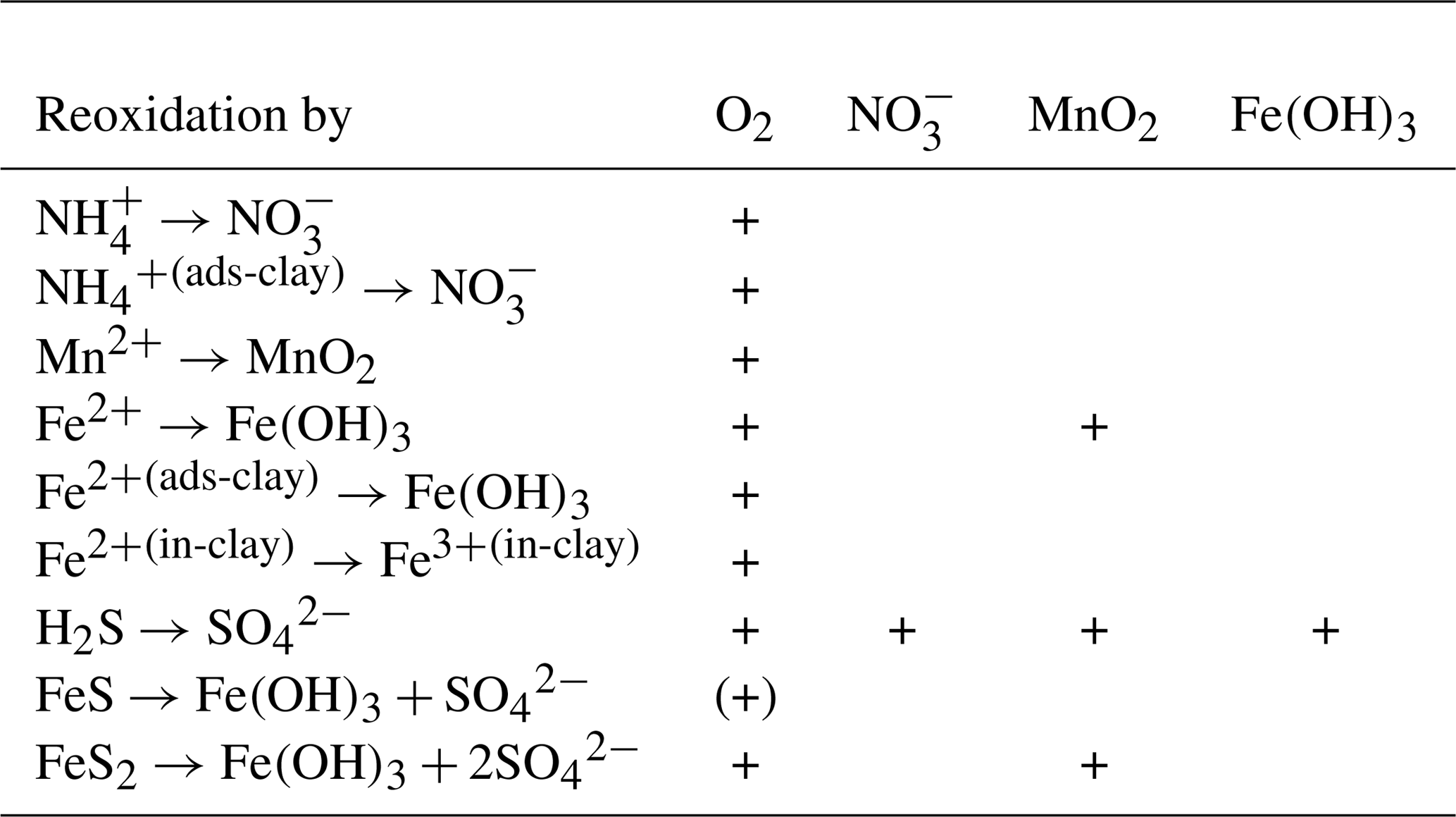
Hydrogen sulfide can reduce any of the previously mentioned oxidants being converted to sulfate. The reaction with oxygen or nitrate is carried out as a two-step reaction. The intermediate species formed in these reactions is elemental sulfur, which can be further oxidised to sulfate. These processes follow the same kinetics as in the water column; see Sect. 2.6.5. Hydrogen sulfide can alternatively react with manganese oxides or iron oxyhydroxides, producing dissolved Mn (II) or Fe (II). For the generated Fe (II), however, we assume either an immediate precipitation to iron monosulfide or an immediate absorption to clay minerals, whichever is more favourable. We assume these reactions to be proportional to both the concentration of sulfide and the metal oxides. Hydrogen sulfide can also reduce structural Fe (III) in the clay minerals, and the Fe (II) will in this case remain in the clay.
This reaction follows process 47 in Table 4. The process runs at a speed of
The model parameter r_i2i_ox describes a relative speed of
0.1 day−1 at which H2S is reoxidised by this process, a somewhat
arbitrary value just expressing our assumption that the process is fast
compared to vertical transport of the clay minerals. The model shows low
sensitivity to this rate parameter, as shown in the Supplement.
The process is Ivlev-limited by the factor li3i.
Iron monosulfide is typically not directly oxidised but dissolves at low sulfide concentrations. However, if it is exposed to oxygen, we assume complete oxidation to Fe (III) and sulfate.
Finally, pyrite can be oxidised in the presence of oxygen or manganese (IV), but in marine environments not by Fe (III) (Schippers and Jørgensen, 2002). We assume complete oxidation to sulfate and iron oxyhydroxides.
2.8 Carbon cycle
The carbon cycle in this model is included, following Millero (1995) and Dickson et al. (2007). Four parameters describe the state of the dissolved carbonate system in the water:
-
pH,
-
total alkalinity (TA),
-
dissolved inorganic carbon concentration (DIC) and
-
CO2 partial pressure (pCO2).
Knowledge of any two of them allows for the determination of the other two parameters. We use TA and DIC as state variables. The reason for this is that both pH and pCO2 can be changed by quick equilibrium reactions with a proton transition, which occurs faster than our model time step allows, while TA and DIC cannot. For details on these reactions, see Dickson et al. (2007).
The DIC concentration can increase by the mineralisation of organic carbon and decrease when DIC is assimilated by phytoplankton. Also, it can be modified by CO2 exchange with the atmosphere. Calcification and carbonate dissolution are not considered in our model. Total alkalinity changes if acidic or alkaline substances are added or removed. The substances occurring in our model approach which change alkalinity are OH−, H3O+ and ions. The effect of dissolved organic matter on total alkalinity (Kuliński et al., 2014; Ulfsbo et al., 2015) is neglected in the present model, but it may be included in a future version.
The tracer value changes by 1 unit if (see Table 1)
-
ohminusis changed by 1 unit, -
h3oplusis changed by −1 unit or -
t_po4is changed by 0.5 units.
As the pH (for adsorption and precipitation reactions) and pCO2 (for gas
exchange with the atmosphere) are of particular importance, we need to derive
these from the state variables. This is done in an iterative procedure.
Starting with a guessed pH value (from the last model time step), we aim to
correct it until it is consistent with the given values of t_alk
and t_dic. To perform this correction, we calculate the
fractionation of DIC into the different species (CO2, ,
). From this, we determine a carbonate alkalinity as , where square brackets denote a
concentration. This can be determined by (Dickson et al., 2007)
where and and are the acid dissociation constants for carbonates as taken from Dickson et al. (2007). We do the same for other substances taking part in acid–base dissociation reactions (water, boron, sulfide, phosphate):
The dissociation constants k are taken from Dickson et al. (2007), and the total boron concentration is calculated from salinity as (Moberg and Harding, 1933)
where S denotes salinity.
The sum of all their alkalinities should then match the total known alkalinity, but a difference occurs because the approximated pH was incorrect.
So, we do a Newton iteration to find an improved pH estimate.
This is done by calculating the derivative
and obtaining the new pH estimate as
We use a fixed number of 10 iteration steps for a better parallel performance of the code.
Finally, we can calculate pCO2 as
2.9 Numerical aspects
The equations which determine the temporal evolution of the state variables are solved by a mode-splitting method; i.e. concentration changes due to physical and biogeochemical processes are applied alternately in separate sub-time steps. For a discussion of this method and alternatives we refer to Butenschön et al. (2012).
2.9.1 Numerics of physical processes
Vertical diffusion is done explicitly by multiplying each vertical tracer vector by a diffusion matrix. This includes turbulent mixing in the water column as well as pore water diffusion, bioturbation (faunal solid transport) and bioirrigation (faunal solute transport). This diffusion matrix is tridiagonal, and for a small time step, which is in our case limited by the thin layers at the top of the sediment, a Euler-forward method can be applied. Larger time steps could be split into smaller Euler-forward steps, which means a repeated multiplication by the tridiagonal matrix. We instead use an efficient algorithm to calculate powers of the tridiagonal matrix (Al-Hassan, 2012) and perform the multiplication only once.
2.9.2 Numerics of biogeochemical processes
The sources and sinks for the different tracers are calculated from the process rates. These include not only biogeochemistry, but also parameterisations for lateral transport processes as well as sedimentation and resuspension.
To calculate the changes in a tracer concentration with time, we form the sum of the processes consuming or producing it (Radtke and Burchard, 2015):
Here, Ti represents the concentration of tracer i, pk is the rate at which process k runs and qik (and sik) is the stoichiometric ratio in which process k produces (or consumes) tracer i. In order to ensure both non-negativity of the tracer concentrations and mass conservation, we apply the positive Euler-forward method from Radtke and Burchard (2015). It is a clipping method which, in the case that a tracer concentration becomes negative during one Euler-forward time step, first executes a partial time step until this tracer is zero. Then the rest of the time step is continued without the processes consuming this tracer, i.e. they are switched off. More than two partial time steps may be needed if more than one tracer is exhausted.
2.10 Automatic code generation
The model code is not handwritten. Instead, the model is described in a formal way in terms of its tracers, constants and processes in a set of text files. The model code is then generated by a code generation tool (CGT) which fills this information into a code template file. The advantage is that the same biogeochemical equations can in this way be integrated into different models. While the current version is written in Pascal, the three-dimensional version in MOM5 has been created as a Fortran code. The CGT is open-source software and can be downloaded at http://www.ergom.net (last access: 10 January 2019).
We use four different observational datasets for model calibration and validation. The data used are (a) pore water profiles for different dissolved species, (b) sediment elemental composition, (c) estimates of bioturbation intensity and (d) bentho-pelagic fluxes measured in benthic chamber lander incubations.
3.1 Selected stations
All data were collected at seven different stations in the southern Baltic Sea (see Fig. 1; we always present the stations from west to east). The mud stations LB and MB are situated in the Mecklenburg Bight, a trough-like bay in the south-western Baltic Sea where salinities are up to 20 g kg−1. Stations ST and DS are on sandy substrate, and the latter one is situated in only 22 m of depth near the major sill, which impedes the transport of the more saline North Sea water into the inner part of the Baltic Sea. Station AB is situated in the central Arkona Basin in 45 m of depth. The Arkona Basin is the most western basin of the inner Baltic Sea. It accumulates organic matter not only from local primary production, but also laterally imported particles from coastal areas experiencing strong eutrophication, especially from the Oder River (Christiansen et al., 2002). Station TW is a silt station with a median grain size around 40 µm. The last station, the sandy station OB on the Oder Bank, is not a place of organic matter deposition, but rather of transformation before the detritus is transported to deeper locations. The Oder Bank is a shallow sandy area strongly influenced by the Oder River plume (Voss and Struck, 1997).
All the stations were sampled during 12 cruises which took place between July 2013 and January 2016 to cover different seasons (Lipka, 2018). However, not every station was sampled during every cruise. The calibration of the model occurred in parallel with the sampling campaign such that only data from the first seven cruises (until January 2015) were used for model fitting.
3.2 Pore water analyses
Short sediment cores with intact sediment–water interfaces were taken by a multicorer, a device which simultaneously extracts eight sediment cores from the sea floor. Pore water was extracted at different depths by rhizones. For a detailed description of the analytical methods used, we refer to Lipka et al. (2018a). Here, we just give a short summary: ammonium concentrations were measured onboard using standard photometric methods (Winde et al., 2014). The quantification of major and trace elements was done on land, following the ICP-OES method (Kowalski et al., 2012). Dissolved inorganic carbon was measured by a mass spectrometer in the gas phase after treatment of the pore water sample with phosphoric acid. Total alkalinity was determined colorimetrically after Sarazin et al. (1999). Dissolved sulfide was determined spectrophotometrically by the methylene blue technique (Cline, 1969).
Instead of directly comparing sulfate concentrations between model and reality, which change over time with salinity, we use the sulfate deficit defined as
where [SO4] and [K] are the measured concentrations of sulfate and potassium (the latter regarded as a passive tracer) in the pore water, and and [K∗] are their typical concentrations in seawater of 35 g kg−1 salinity (Dickson and Goyet, 1994).
3.3 Sediment composition
Parallel sediment cores from the same multicorer casts as used for the pore water analysis were subsampled in 1 cm steps, freeze-dried under vacuum and homogenised for geochemical analyses. Total carbon (TC) as well as nitrogen (TN) and sulfur (TS) contents were measured by combustion, chromatographical separation of the released gases and their determination with a thermal conductivity detector. The total inorganic carbon (TIC) content was measured by acidic removal of carbonates and analysis of the released CO2 with a nondispersive infrared detector. The total organic carbon (TOC) content was then calculated by the subtraction of TIC from TC values. At the sand stations (ST, DS and OB), the mass fractions were measured in the fine fraction (<63 µm) of the sediment only, assuming that the coarse fraction does not contain these elements in a significant amount. Thus, the percentage in the whole sediment was calculated by multiplying with the fine fraction ratio that was determined by laser diffractometry. Analytical details related to the devices used, their calibration, and precision and accuracy can be obtained from Bunke (2018).
3.4 Bioturbation intensity estimates
In order to analyse bioturbation intensities (DB), 6 to 24 cores per station were sliced onboard immediately after retrieval at 0.5 cm intervals to 3 cm of depth and at 1 cm intervals to 10 cm for vertical chlorophyll a (Chl a) profiles. All samples were deep-frozen (−18 ∘C) and stored until extraction (Sun et al., 1991). In the laboratory, the defrosted sediment samples were homogenised and three parallel subsamples of 1 cm3 volume were taken from each slice. After adding 9 mL of 96 % ethanol and an incubation period of 24 h in the dark, the samples were centrifuged at 4000 rpm for 5 min and measured photometrically (663 and 750 nm); chlorophyll was calculated based on HELCOM (1988). The vertical chlorophyll profiles were interpreted using the bio-mixing model developed by Soetaert et al. (1996b). Experimentally derived chlorophyll decay constants of 0.01 day−1 for mud and 0.02 day−1 for sand (Morys, 2016), and an artificially small sedimentation rate ω of 0.00001 cm day−1, were used, the latter just reflecting the fact that chlorophyll decay is much faster than sedimentation. The model applied may distinguish between diffusive and non-diffusive mixing. The latter mode of bioturbation was neglected in our study despite the fact that it may be the dominant particle transport process in certain areas (e.g. AB).
3.5 Bentho-pelagic fluxes
Total oxygen uptake (TOU) and bentho-pelagic nutrient fluxes (, , ) of the sediments were measured in situ with two identical benthic lander systems, each a “mini benthic chamber” courtesy of Stefan Sommer and Peter Linke (GEOMAR Kiel, Germany) during cruises AL434, EMB076, POS475, EMB100 and EMB111 (Lipka, 2018). All systems were equipped with a Plexiglas® chamber (diameter 19 cm), an electronically driven glass syringe water sampler and oxygen optodes (Aanderaa Instruments, Norway; no. 4831) inside and outside of the chamber. The oxygen concentration trend was used as the main parameter for gas fluidity and tightness. Each respective chamber covers a sediment area of 284 cm2 and the chamber water volume was in the range of 5–8 L depending on sediment penetration depth. Incubation times at the sea floor ranged from 9 to 48 h. Discrete chamber water samples were gathered by up to eight glass syringes (volume approx. 45 mL) in intervals of 1–7 h, depending on total deployment time. Photo lights (SolaDive 1200) and a photo camera (GoPro Hero Black Edition 3+) were used for the observation of the chamber deployment, particularly to check for sediment disruption. The start of incubation was defined if initial concentrations inside the chamber were close to bottom water concentrations. Nutrient concentrations were measured with a QuAAtro multianalyser system (Seal Analytical, Southampton, UK) onboard using standard photometric methods (Grasshoff et al., 2009). Nutrient fluxes were calculated from the linear increase or decrease in concentration versus time, corrected for the surface-area-to-volume ratio of each chamber. A robust linear regression method which is tolerant to outliers was applied (Huber, 1981; Venables and Ripley, 2002), and the uncertainties of the fluxes were obtained by an ordinary bootstrapping approach (Canty and Ripley, 2017; Davison and Hinkley, 1997). The regression analysis to determine their fluxes was performed in the same way as for the nutrients. TOU was calculated by standard linear regression of O2 concentration versus time (with R2 values above 0.98) within a period, while O2 concentration did not sink below 15 % of the initial concentration (Glud, 2008). Calibrations of O2 optodes were performed in ambient seawater aerated for 30 min (100 % atmospheric saturation) and in saturated seawater – sodium dithionite solution (0 % oxygen), regularly cross-checked by Winkler titration (Winkler, 1888).
Kersten et al. (2005)Leipe et al. (2011)Emeis et al. (2002)Table 7Porosity and sediment accumulation rate data used as model input and clay volume content estimated by the model based on an initial guess.
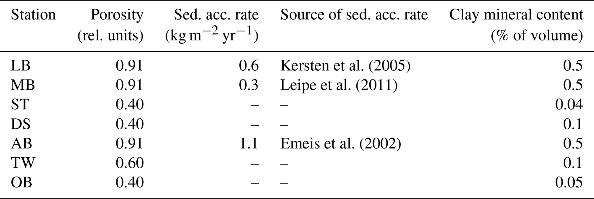
There are three ways in which observations feed into our model:
-
model constants which were derived in earlier studies and which our model adopted from previous models;
-
initial and boundary conditions determining tracer concentrations at the beginning and throughout the model run; and
-
calibration data which help to confine uncertain model parameters during a repeated model calibration process.
4.1 Use of data as model constants
Most of the observations which help constrain our model processes enter our model indirectly, since model constants are inherited from ancestor models. Especially in van Cappellen and Wang (1996), a thorough confinement of model constants based on observations was achieved. We add to that by supplying site-specific observations for porosity for all seven stations, set to a homogeneous value per substrate type estimated from measurements within the SECOS project (Lipka et al., 2018b). The assumption of a homogenous value is a first approximation motivated by the future aim to use the model in a three-dimensional context. While detailed spatial maps of surface porosity exist, vertical profiles are rare. The effect of this simplification is discussed in Appendix D. Sediment growth estimations for the three muddy sites are taken from different sources, as shown in Table 7.
4.2 Initial and boundary conditions
The initial conditions for most biogeochemical state variables in the water column are taken from the previous run of a three-dimensional ERGOM model as described in Sect. 2.2 (Neumann et al., 2017), which contained a simplified sediment model as described e.g. in Radtke et al. (2012). Concentrations of sulfate and calcium were set to salinity-determined values as described by the standard composition of sea salt (Turekian, 1968). Dissolved dinitrogen was initialised at 100 % saturation (Hamme and Emerson, 2004).
In contrast, fluff and sediment were initialised empty. We allowed them to fill up with material derived from the water column during the simulated period of 100 years. While this period of 100 years is not sufficient to fill the considered 22 cm of sediment by accumulation, it is sufficient to almost reach a steady state in the pore water concentrations. While the sixth class of detritus, which is considered non-biodegradable, continues accumulating in the sediments after 100 years, those classes which affect the pore water concentrations decay on smaller timescales.
Since the model conserves nitrogen and phosphorus, the filling of the sediments would have led to a depletion in the water column. To overcome this, we relax the winter concentrations of dissolved inorganic nitrogen and phosphorus (DIN and DIP) against values obtained from the previous 3-D model run. This relaxation is applied every winter, so the nutrients required to fill the model domain are provided from an artificial external source. Their input is large at the beginning of the model run and decreases over time as the sediment reaches a state which is almost in equilibrium with the organic matter supply from the water column above.
4.3 Model fit to observed data
Pore water profiles from Lipka (2018) were then used to calibrate the model. The calibration included optimising model parameters for individual stations, as well as parameters for the whole model domain. Typically, this type of calibration is done manually by the modeller. But due to the large number of parameters to optimise (115 in total), we decided to do a systematic, algorithm-based optimisation.
Please note that the physical input data and initial conditions used during the model optimisation phase were taken from a preliminary, unpublished 3-D model run. It differs from the cited model version (Neumann et al., 2017) by using a less realistic light model. Furthermore, dissolved organic nitrogen is not included as a state variable. These improvements were made to the ERGOM model during the development phase of the sediment model, and the results of the sediment model show only small differences between the model versions. We use the data from the final, published 3-D model run for the results shown in this article for reasons of reproducibility. The preliminary forcing data used during the calibration phase are, however, also given in the Supplement.
4.3.1 Penalty function
The first step in such an optimisation is to define a metric or a penalty function quantifying the misfit between model and observations. Our aim is then to minimise this function.
We chose to penalise the relative deviation between model and measurement and define the penalty function by
Here, imax is the number of state variables we compare and jmax(i) is the number of observations of this state variable at all depths and at all stations. The expression ri,j is a measure for the relative deviation between model value mi,j and observation oi,j:
The term Δi15 is included to avoid huge relative errors between values which are close to zero. It denotes the random deviation in this parameter, quantified from duplicate or triplicate measurements of the same parameter in different sediment cores of the same sampling. Obviously ri,j becomes zero if the model and observations match. Finally, the weight wi assigned to each comparison in Eq. (48) is defined as the ratio
between the average observed value of the variable and the random deviation. The weight is applied to make sure that fitting the most certain variables has the highest priority.
The pore water species fitted are ammonium, phosphate, silicate, sulfide, iron, manganese, the total alkalinity and the relative sulfate deficit16.
4.3.2 Optimisation strategies
After we defined a penalty function, the second step is to choose an algorithm to minimise it. Several such algorithms exist; however, our choice of methods was restricted by the relatively long runtime of a single model iteration. Since it took about 8 min to run a single station for 100 years, we had to choose methods which
-
needed a relatively small number of iteration steps and therefore
-
allowed for a high degree of parallelism in the individual optimisation step in order to effectively search the 115-dimensional parameter space.
Our first choice was the Adaptive Hierarchical Recombination–Evolutionary Strategies (AHR-ES) algorithm implemented in the R package calibraR (Oliveros-Ramos and Shin, 2016). We were, however, not satisfied with the optimisation result. Possibly we just failed to find out the optimal settings for the algorithm, such as the survival rate.
Therefore, our second choice was a simple alternative algorithm: our own extension of the generalised pattern search (GPS) algorithm (Hooke and Jeeves, 1961). Every optimisation step consists of two sub-steps. The first sub-step is the most simple “grid search” step in which all 115 parameters are varied by a predefined step width. We run 230 sets of seven models in parallel such that each parameter can be both increased and decreased. In the second sub-step, 230 combinations of the most successful changes are formed. Even if no single parameter change could improve the existing solution, sometimes combinations of them can, which is the basic idea of GPS. The parameter vector with the best score which was obtained in any of the two sub-steps is then chosen as the starting point for the next step. If neither of the two sub-steps leads to an improvement of the overall fit, the step size is reduced by a factor of 2.
The optimisation converged after 30 iteration steps and reduced the error function from 6363 (the value obtained by previous manual tuning) to 4797.
The algorithm obviously does not guarantee that we reach a global optimum, which can be seen as a drawback. The automatic method was started after manual calibration of the model. Since the optimisation method is deterministic, the local optimum is defined by this initial condition. However, in a vector space with a dimension as high as ours, it is anyway difficult to find a non-local point with a better score, no matter if it is by manual optimisation or a different search algorithm.
4.4 Manual correction of sand and silt stations
For the sand stations and the single silt station, the automatic optimisation resulted in an unrealistic set of parameters. The bioturbation rates were estimated as low as those of the mud stations. However, at these low bioturbation rates, the sediments failed to accumulate realistic amounts of organic matter. The pore water profiles we obtained, however, seemed to match the observations relatively well. This was due to the fact that the realistically low concentrations of solute species were obtained by an unrealistically low incorporation of degradable particulate material into the sediments. The model assumed relatively high rates of lateral removal of fluff such that only a small fraction of the locally produced detritus was actually processed in the sediments.
This illustrates the problem that if the diffusivity is unknown, very
different transports can be caused by the same pore water gradient. We
therefore decided to manually modify the solution. This modification meant
raising bioturbation and bioirrigation intensity by a factor of 10 at each
station. Afterwards we reduced the parameter r_fluffy_moveaway,
which describes the rate at which fluff layer material is transported to the
deeper areas until realistic concentrations in the pore water profiles were
reached.
This led to similar pore water profiles, but higher turnover rates and organic content in the sediments.
5.1 Comparison to measured pore water profiles
In this section, we compare and discuss the observed and simulated pore water profiles of several chemical species relevant for early diagenetic processes. Model results are taken from the last year of the 100-year simulation, which was driven by a repeated forcing every year. After this simulated period, the model almost reached a quasi-steady state, which means the annual cycle of pore water concentrations was nearly repeated year after year at each of the stations. The sixth class of detritus, in contrast, which we defined as non-degradable, did not reach a stable concentration, but continued to accumulate in the sediment during the period of 100 years, but this continued accumulation did not influence the pore water profiles due to the fact that it was assumed to be bioinert.
5.1.1 Pore water profiles at mud stations
Figure 4 shows a comparison of simulated and measured pore water profiles at the three mud stations.
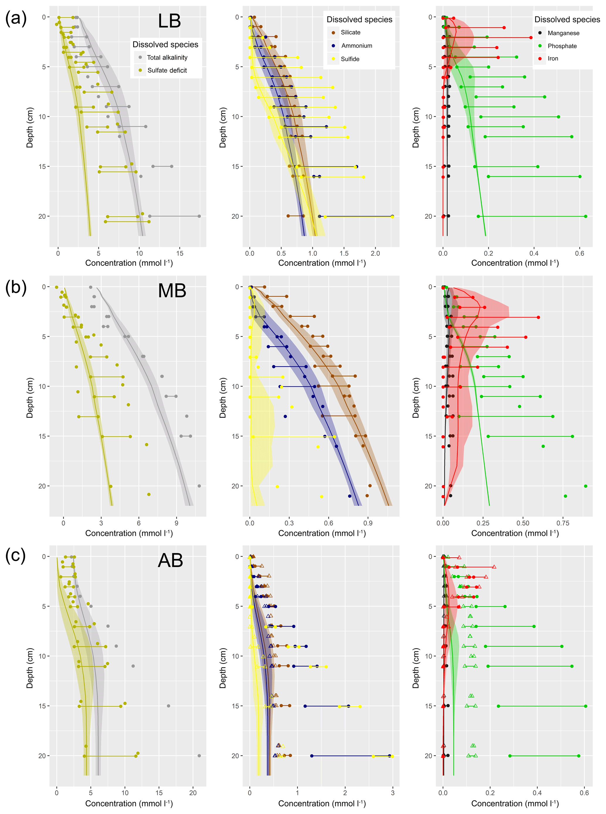
Figure 4Pore water concentrations of several dissolved species at the three mud stations Lübeck Bight (a), Mecklenburg Bight (b) and Arkona Basin (c). Points and horizontal lines indicate the range of measurements. For station AB, open triangles indicate the range of observations from the January 2015 cruise, which were taken at a different location in the same area 23 km apart. Curves and shading present the model results and indicate year-average concentrations and the seasonal range. Please note the different horizontal scales.
In the left panels, we see that the rise of alkalinity with depth is captured well by the model, except for the AB site where observations show a higher alkalinity below 10 cm of depth. The decline in sulfate follows the lower range of the observations.
The panels in the second column show that the vertical profiles of ammonium and silicate are also represented relatively well by the model. However, especially at the Arkona Basin station, the observed range of both ammonium and sulfide shows strong variation (by an order of magnitude). The model does not capture that but rather sticks to the lower range of the observations. Most probably, the variability in the observations is not due to seasonality, but a consequence of spatial variability between sampling sites, since the samples were taken from two sites 23 km apart.
Surprisingly, the model is able to reflect the differently steep sulfide profiles between the stations LB and MB. While Lipka (2018) see the low sulfide concentrations which occur especially in March 2014 at MB as an indication for a preceding mixing event, our model cannot adopt this interpretation due to its limitation by a temporally constant vertical mixing. In contrast, our model suggests a higher deposition of iron oxyhydroxides at this site.
The right panels show that the modelled manganese concentrations match the observations quite well. The dissolved iron profiles show their maxima at the correct depths and a relatively large seasonal spread. The measurements show an even larger spread than the model. For the phosphate profiles, the model results mostly resemble the lowest of the measured values, except for station AB where we see a clear underestimation. This can be seen as an artefact of our fitting method, more precisely of the choice of our penalty function. Giving a penalty for the relative error means that the same absolute error is punished more heavily if the observation is smaller, making the model try harder to fit low values compared to high ones.
The model results for the mud stations fit quite well, considering the fact that the real pore water profiles may be shaped by very different temporal variations. These include, for example, mixing events, changing loads of organic matter, or temperature and salinity variations. Our model, not knowing the sediments' past, can only try to estimate the average conditions that might produce similar pore water concentrations.
5.1.2 Pore water profiles at sand stations
Figure 5 illustrates the model fit at the sandy stations.
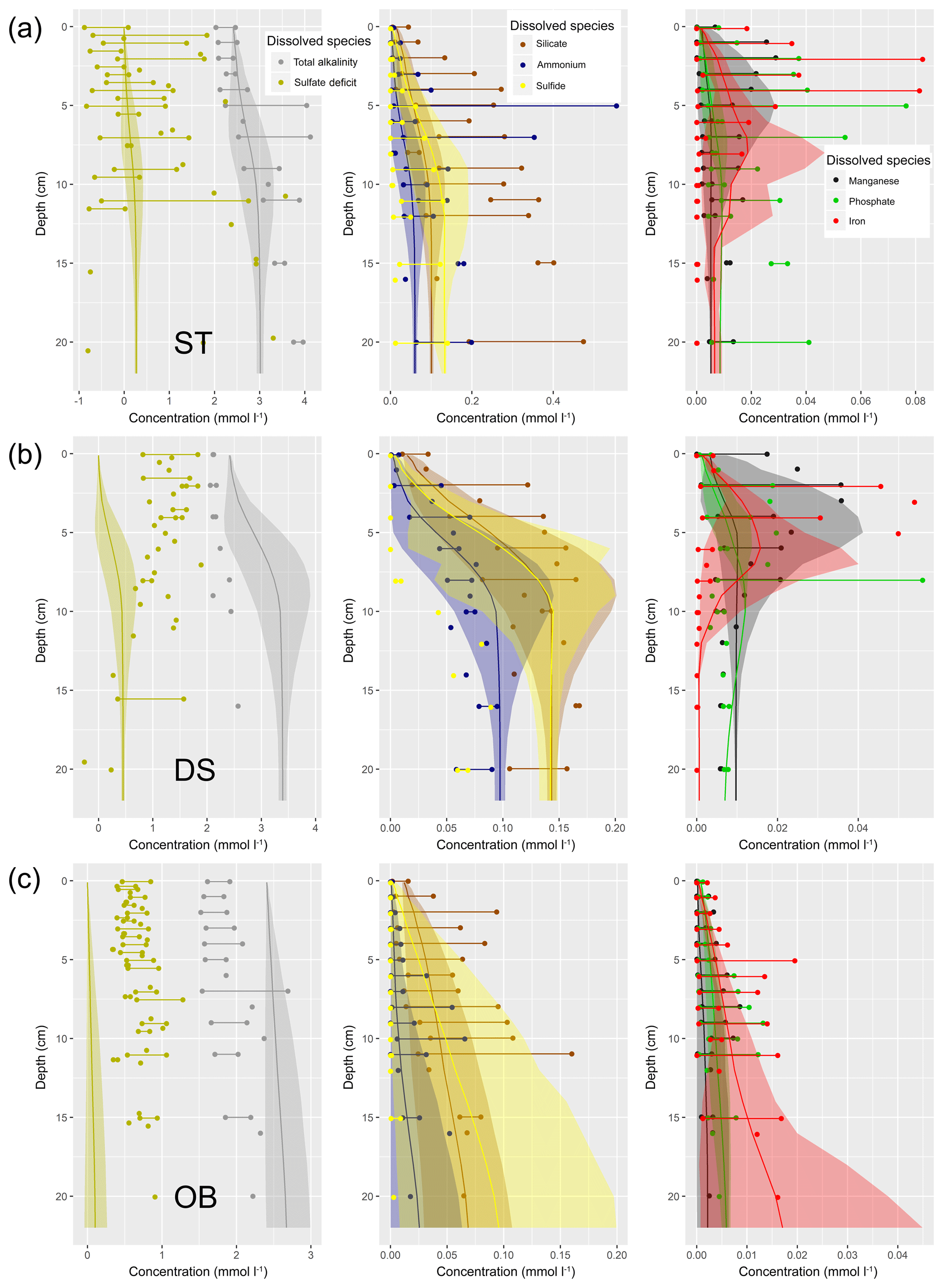
Figure 5Pore water concentrations of several dissolved species at the three sand stations Stoltera (a), Darss Sill (b) and Oder Bank (c). Points and horizontal lines indicate the range of measurements. Curves and shading present the model results and indicate year-average concentrations and the seasonal range. Please note the different horizontal scales.
All of the sandy stations have one major error in common: sulfide concentrations are strongly overestimated at depths below 5 cm. We suppose that the precipitation or reoxidation of sulfide is underestimated. For all other pore water species, the agreement between measured and modelled ranges is reasonable. The rise of alkalinity with depth is especially well captured by the model. The sulfate deficit in the empirical data has a large uncertainty, as it is calculated as a small difference of similarly large quantities.
In our model, the sandy sites show a more pronounced seasonal cycle in the pore water profiles compared to the muddy stations. Especially iron and manganese concentrations vary considerably due to the seasonally different supply of quickly degradable organic matter and corresponding differences in mixing intensity. While the variability in the supply of fresh organic matter is captured by the model, the variation in mixing is not. Still, the simulated ranges are supported by the variability in the observed pore water concentrations.
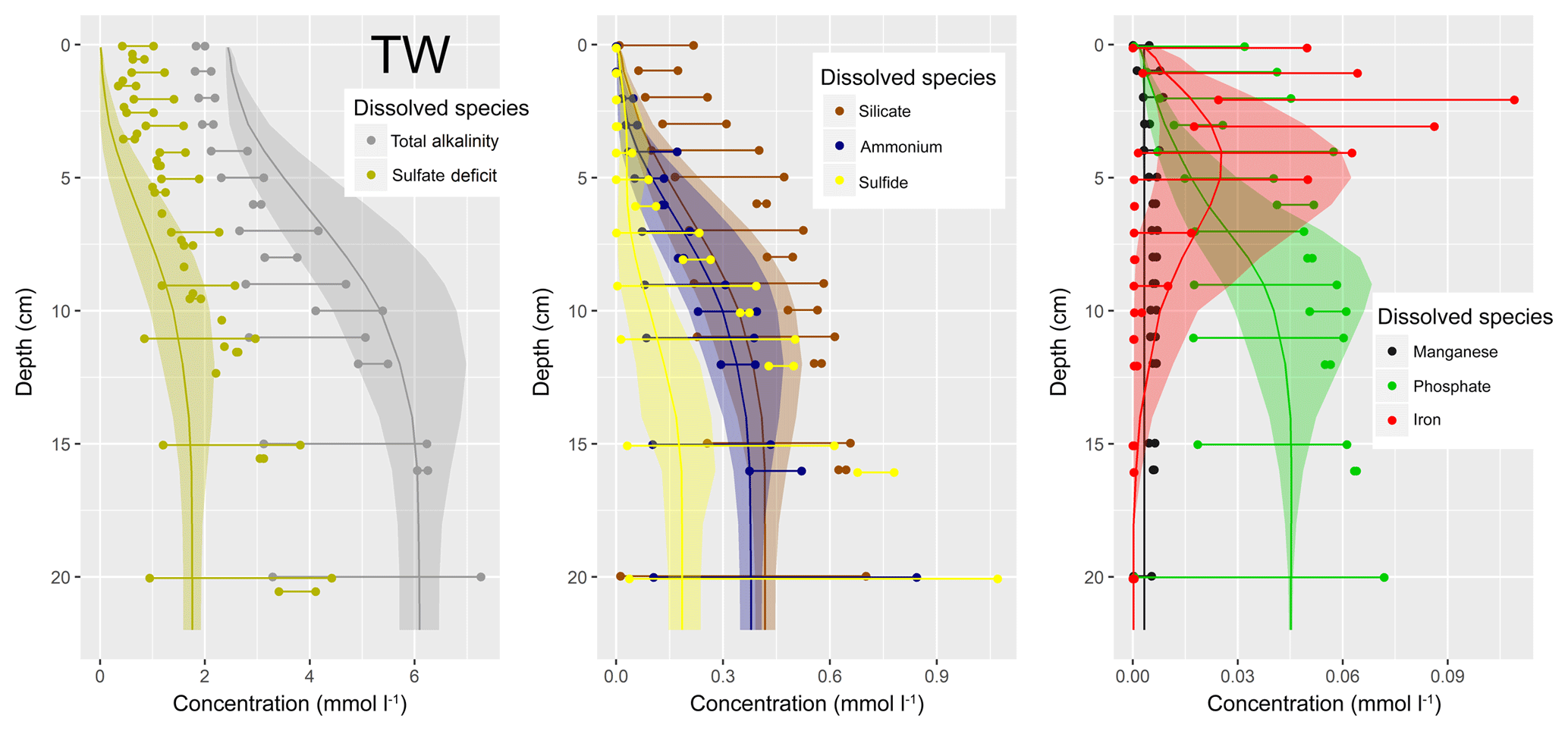
Figure 6Pore water concentrations of several dissolved species at the silt station Tromper Wiek. Points and horizontal lines indicate the range of measurements. Curves and shading present the model results and indicate year-average concentrations and the seasonal range.
5.1.3 Pore water profiles at the silt station Tromper Wiek
For the station Tromper Wiek, we used data from two different cruises in April and June 2014. Even if the idea in the SECOS project was to repeatedly sample the same station, the locations were approximately 6 km apart for this station, and the substrate type at the station sampled in April was sand rather than silt. The amount of sulfide in the pore waters showed a large difference between the April and the June cruise, with the latter concentrations exceeding the former by a factor of 20. This reflects spatial rather than temporal variations. Some of the depth intervals were only sampled during the June cruise, which explains the different observed ranges at the different depths.
The good agreement in the profiles of ammonium and phosphate (middle and right panel in Fig. 6) suggests that total mineralisation is captured well. The left panel shows that the model estimates the sulfate deficit at the lower range of observations, but the rise of alkalinity with depth at the higher range. The model overestimates the vertical extent of Fe (II) in the pore waters. However, the model reasonably reproduced the range of iron concentrations and also the fact that dissolved manganese concentrations were always low compared to those of iron.
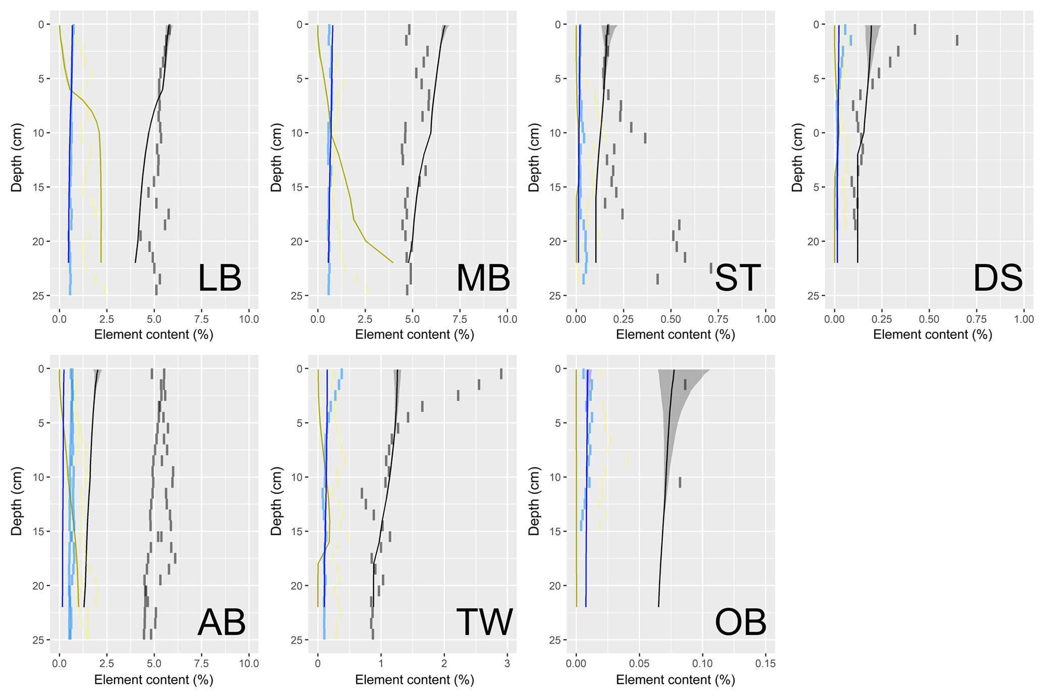
Figure 7Mass fractions of nitrogen (blue), sulfur (yellow) and organic carbon (black) in the dry sediment: model results (curves and shading for seasonal range) versus measurements (vertical segments). Please note that the scales on the horizontal axes differ by a factor of 40.
5.2 Comparison to sediment composition estimates
In Fig. 7, we compare the composition of the solid parts of the sediment between model and measurements.
For the mud stations LB and MB, the modelled element concentrations show a quantitative agreement with the measurements. The main difference is that the measured values show strong vertical fluctuations, which may be the result of the deposition history. Another difference is that the vertical gradients of sulfur are considerably steeper in the model than in reality. In the mud station AB (Arkona Basin), however, the actual concentrations of all three elements are heavily underestimated. Nonetheless, the depth gradients of the concentrations match quite well, so there is perhaps just a constant offset. This might be caused by the accumulation of bioinert organic material, possibly of terrigenous origin from the Oder River.
In all sand stations (ST, DS, OB), the amount of sulfur in the sediments is underestimated. The observed sulfur in the sediments varies with depth and shows a maximum at around 10 cm of depth. The fact that sulfide, in contrast, was overestimated in the pore waters, suggests that the precipitation of sulfur may be underestimated in the sandy cores. Particulate N and TOC are present in realistic quantities at the OB station. At the other two sand stations, the N and TOC observations show maxima at the top (station DS) or bottom (station ST) of the profile, which are not captured by the model. These are most likely the traces of past sedimentation or bioturbation events.
Reproducing subsurface TOC maxima, as they occur in permeable sediments, represents a challenge for early diagenetic models. They can be caused by different processes, such as
-
non-local, fauna-driven ingestion of fluff material into a specific depth,
-
washout of organic material from the surface sediment e.g. during storm events or
-
lateral relocation of sediments.
5.3 Comparison to measured bioturbation intensities
The empirically estimated bioturbation intensities span a large range at each station. A reason for this may be that while our model assumes a temporally constant bioturbation, in reality it is highly variable. Mixing events by animals or shear stress alternate with periods without mixing (Meysman et al., 2008). Investigations of individual cores can only give snapshots of this highly variable mixing rate.
In Fig. 8a, we compare measured bioturbation diffusivities DB to those used in the model. Since the observed ranges are very large, they almost always contain the value assumed in the model. An exception is the Tromper Wiek site where exceptionally high DB values were measured. This may, however, be an artefact based on the method of calculating the diffusivities. While we assume diffusion–analogue mixing in the model, non-local mixing also occurs in nature. The two processes can be distinguished from the analysis of Chl a profiles (Morys et al., 2016; Soetaert et al., 1996b). Figure 8b shows how often the samples from a specific site supported the hypothesis of diffusion–analogue mixing. For the station TW, it was only one-fourth of the sediment cores that could be explained assuming local mixing, so non-local mixing was identified as a major process here. DB values were only calculated for cores in which the observed Chl a profiles could be explained by local mixing alone.
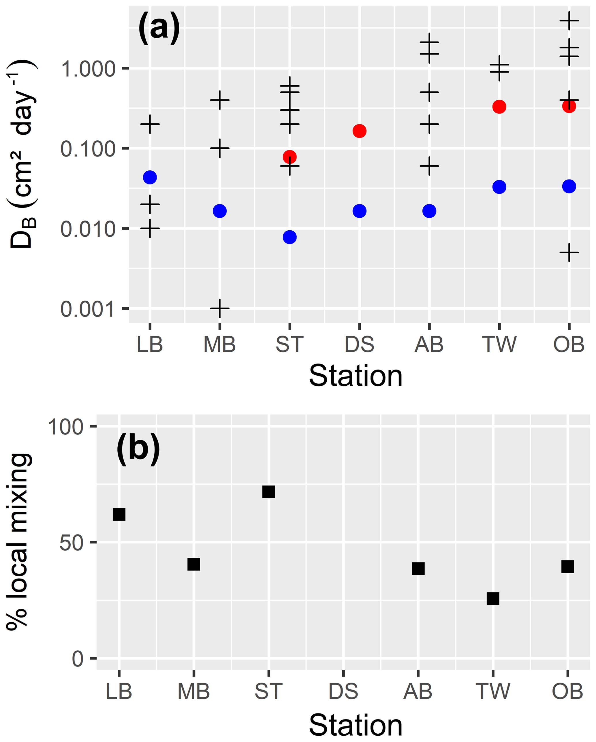
Figure 8(a) Model estimations of bioturbation intensity (blue dots) manually corrected for sand and silt stations (red dots) and Chl a-based estimates (black crosses); data from Morys et al. (2016). Black crosses represent averages over all cores from a single month when the Chl a profiles in the sediment support the assumption of diffusion–analogue mixing. So, variation can be interpreted as temporal variability. (b) The percentage of the cores at this station whose Chl a profiles could be explained by the assumption of a local diffusion–analogue mixing process.
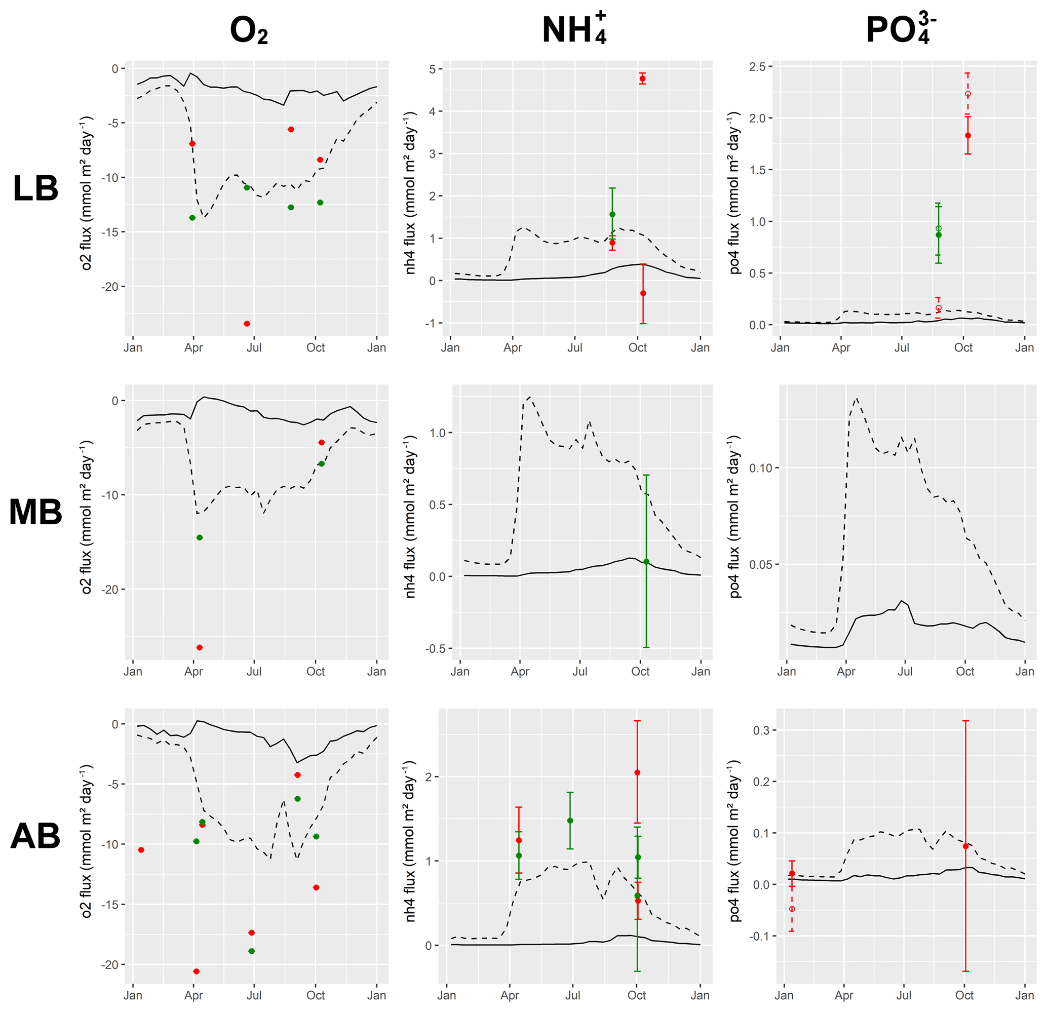
Figure 9Fluxes between the sediment and bottom water of selected pore water species at mud stations. Positive values denote fluxes out of the sediment. Solid line: modelled fluxes between sediment and bottom water only. Dashed line: fluxes including mineralisation of the fluff layer material. Dots: measured fluxes by two benthic chambers (BC1 in red and BC2 in green). Vertical ranges: uncertainties of these fluxes estimated by a bootstrapping method. For phosphate: full circles are estimates based on phosphate determination by photometric methods, and open circles are estimates based on P quantification by the ICP-OES method.
The automatic model calibration yielded diffusivities at the sand and silt stations which were as low as those at the mud stations. Such weak mixing, however, could not supply enough organic matter to the sediments to reach measured element compositions. Therefore, they were corrected upwards, resulting in higher mixing at the sandy than at the muddy sites. This agrees with recent estimates of the bioturbation potential (Gogina et al., 2017; Morys et al., 2017), an index describing the ability of macrofauna to displace sediment particles, resulting in a mixing effect. This potential was estimated to be higher in the more shallow sandy areas than in the muds. Also, measured bioturbation rates in the SECOS project were higher in the sand than in the mud (Morys, 2019). However, the high variability of bioturbation rates within stations makes it difficult to prove a significant difference in DB between sandy and muddy areas empirically (Morys et al., 2016).
5.4 Comparison to measured bentho-pelagic fluxes
The net fluxes of selected pore water species (O2, and ) into the sediment or out of it are shown in Figs. 9 and 10 for mud and sand–silt stations, respectively. An additional figure showing the fluxes of DIC, , Fe, Si and is given in the Supplement. The figures compare modelled fluxes to observations from benthic chamber lander incubations. For each of the selected species, we get two contributions in the model: the flux into or out of the sediment itself (diffusive and by bioirrigation) and a consumption or production by mineralisation of the fluff layer material. We can distinguish these in the model, but not in the measurements, because (a) the benthic chamber lander measures concentration changes in the bottom water only and (b) at the mud stations, the border between sediment and the fluff layer is a smooth transition rather than a discrete boundary.

Figure 10Fluxes between the sediment and bottom water of selected pore water species at sand stations. Positive values denote fluxes out of the sediment. Solid line: modelled fluxes between sediment and bottom water only. Dashed line: fluxes including mineralisation of the fluff layer material. Dots: measured fluxes by two benthic chambers (BC1 in red and BC2 in green). Vertical ranges: uncertainties of these fluxes estimated by a bootstrapping method. For phosphate: full circles are estimates based on phosphate determination by photometric methods, and open circles are estimates based on P quantification by the ICP-OES method.
The comparison of annual average oxygen fluxes between the model and measurements shows a reasonable quantitative agreement. Taking the rather high fluctuations in the measurements into account, we cannot assume a perfect fit. The model correctly reproduces the fact that similar oxygen consumption occurs at sand and mud stations in spite of their order-of-magnitude differences in organic content and pore water concentrations (Boudreau et al., 2001). The strong seasonality in the model, with O2 consumption being high during summer and low during winter, cannot be confirmed by the measurements, but we need to state that only two valid measurements exist during January and February when the modelled consumption rates are lowest. For the nutrients, we find highly variable fluxes in the observations, some of which show large relative uncertainties. The model results are in reasonable quantitative agreement with these fluxes, but again the clear seasonality in the model cannot be confirmed empirically. The peak values of the observed fluxes (more than 4 mmol m−2 day−1 for and 2 mmol m−2 day−1 for ) are also much larger than those in the model. Our model also does not show ammonium or phosphate fluxes directed into the sediments, as they occur in a small fraction of the observations. So, we can state that the modelled fluxes are more smooth than the observed ones. This may either reflect reduced spatio-temporal variability in the model or artificial variability introduced into the measurements by the sediment disturbance which our incubation method causes.
5.5 Scope of model applicability and model limitations
In this paper, we applied our model in a one-dimensional context. The aim was to reproduce early diagenetic processes taking place in the sediments at seven exemplary sites thought to be representative for the south-western Baltic Sea by a mechanistic model. In our fully coupled model, the pelagic biogeochemistry and an assumed lateral transport supplied the organic material which drove the early diagenetic processes in the sediments. A comparison to a variety of different observations showed that the model gives a reasonable reconstruction of sediment biogeochemistry. Still, we found differences in the details. For example, a strong overestimation of sulfide concentrations in sandy sediment pore waters most likely points to the underestimation of sulfide precipitation–reoxidation.
The analysis we show suggests that the processes most relevant for these observations are adequately represented in the model. This does not include all parts of the model. For example, the nitrogen cycle was not compared to observations, which is due to the fact that the project SECOS, in which this work was done, did not focus on it and so the required observations of nitrification or denitrification rates are missing.
The ultimate aim of the model is its application in a fully coupled three-dimensional framework. A fully coupled pelagic and benthic model could answer a wide range of questions such as the following.
-
Are the strongly simplifying sediment parameterisations which we use in marine ecosystem models today consistent with our understanding of sediment biogeochemistry, or is there a mismatch between our assumptions in the pelagic models and the sediment–water fluxes in early diagenetic models, which are directly constrained by observational data?
-
How might sedimentary services such as nutrient removal change under different conditions, and what feedbacks into pelagic biogeochemistry can be expected?
-
On which timescales can organic material stored in the sediments affect the eutrophication status of the pelagic ecosystem, e.g. for how long will sedimentary nutrient release counteract nutrient abatement measures aimed at reducing the winter nutrient concentrations in the water column?
The applicability of the one-dimensional model is limited. There is little added value in using this coupled benthic–pelagic model compared to a classical early diagenetic model, since in most cases a one-dimensional description of a pelagic ecosystem will be strongly oversimplified. One could, however, imagine that it can be useful for enclosed marine areas where the horizontal exchange is limited or well known. An application to an area other than the south-western Baltic Sea will, however, require a new model calibration, since critical parameters like bioturbation intensity might differ. We strongly discourage the use of the model as it is by just applying it to derive estimates of benthic biogeochemical process rates from pelagic biogeochemistry unless there is a large set of benthic data available against which the model can be validated.
In cases in which these data are available, we think that the model system has high potential to serve as a starting point for detailed studies because it can be easily modified. Adding, removing or adapting processes is very easy because of the automatic code generation principle. Only a formal mathematical formulation of the process is required, and no coding skills are needed to e.g. add additional state variables to the model system. Reuse of parts of the model, e.g. the explicit representation of the fluff layer, is also possible.
In this paper, we describe an integrated model for ocean biogeochemistry. It simulates ocean biogeochemistry both in the water column and in the sediments.
The model was obtained by combining two ancestor models: the water column model ERGOM (Neumann et al., 2017) and the early diagenetic model used in Reed et al. (2011). A few modifications were made to the existing models, partly to include additional processes relevant for the area of interest, the south-western Baltic Sea. These model extensions include
-
closing the carbon cycle in the sediments, which allows for the determination of pH,
-
adding a specific numerical scheme for the diffusion of the tracer “total alkalinity”,
-
using ion activities rather than concentrations to determine precipitation and dissolution potentials, allowing us to account for salinity differences,
-
the explicit description of adsorption to clay minerals considering their mineralogy, and
-
an alternative pyrite formation pathway via H2 formation.
An automated model calibration approach was used to fit the model to pore water observations at seven sites in the study area. It was successful for the mud stations, but underestimated bioturbation rates and consequently the organic content of the sediment at the sand and silt sites. Therefore, these model parameters were adjusted manually at the sand and silt sites. This issue illustrates a general problem related to models of this complexity. The large quantity of unknown model parameters results in many degrees of freedom, and different types of observations are needed to constrain them. Even so, a good fit to a constrained set of observations does not guarantee that the model dynamics are captured realistically.
Applying the model in a three-dimensional framework (Cahill et al., 2019) will reduce the degrees of freedom. For example, our model includes parameterisations for (a) lateral removal of fluff material from the sand stations and (b) lateral import of organic material at the mud stations. In a 3-D ocean model, these become intrinsically linked by the constraint of mass conservation. Other degrees of freedom arise from the supply of oxidised iron and manganese to the individual stations. In a 3-D model, the supply and distribution of these substances would be controlled by erosion and deposition and thus determined by the model physics.
Apart from these constraints, the implementation of the model in a 3-D framework is straightforward. Physically, the coupling between different locations would be controlled by the fluff layer and its erosion and redeposition. Technically, the coupling is simplified due to the use of automatic code generation. Describing the model processes and constants in a formal way, keeping them separate from code for specific models, means it is easy to switch between different “host models”. The major difficulty in going 3-D is the limited amount of validation data, such as pore water profiles and sediment–water fluxes, compared to the strong spatial and temporal variability. A first step is the application of the model to the limited area of the German EEZ for which the model is calibrated.
In the long term, biogeochemical ocean models should aim at a process-resolving description of surface sediments. This is especially true for shallow ocean areas where the efflux of nutrients from the sediment strongly influences water column biogeochemistry, like in our study area. The magnitudes of denitrification and phosphate retention, or the spatial and seasonal patterns in which oxygen consumption occurs, may strongly influence marine ecosystems.
Very often, model studies discussing “what if” scenarios use a relatively simple sediment representation. This includes studies on nutrient abatement, human-induced stresses on ecosystems (e.g. by fish farming) and climate sensitivity analyses. But the use of a present-day parameterisation for future scenarios means a neglect of possible changes. In the context of limited data and process understanding, this implicit “no-change” assumption may be the best we can presently do. But we should be aware of the uncertainty introduced by this pragmatic choice. Studying the sensitivity of sediment functions to external drivers in a process-resolving sediment model can be a way to quantify these uncertainties and possibly derive an ensemble of alternative future parameterisations.
A source code version of the model can be obtained from Radtke (2018) and is also provided in the Supplement to this article. The Supplement includes the initial conditions and physical forcing files required to reproduce the obtained results.
The code is not handwritten, but can be generated automatically from a set of text files describing the model biogeochemistry and a code template containing the physical and numerical aspects of the model code. All three ingredients required to obtain the model source code (the text files, the code template and the code generator program) are also included.
These components in their current and previous versions are GPLv3 licenced and can also be downloaded from our website at http://www.ergom.net.
For the calibration and validation data used in this study, we refer to the following publications: the pore water data can be found in Lipka (2018); the sediment composition data are published in Bunke (2018); and the bioturbation rate estimates are available in Morys (2016).
The stoichiometric composition of the model tracers is shown in Table A1.
Table A1Stoichiometric composition of tracers.
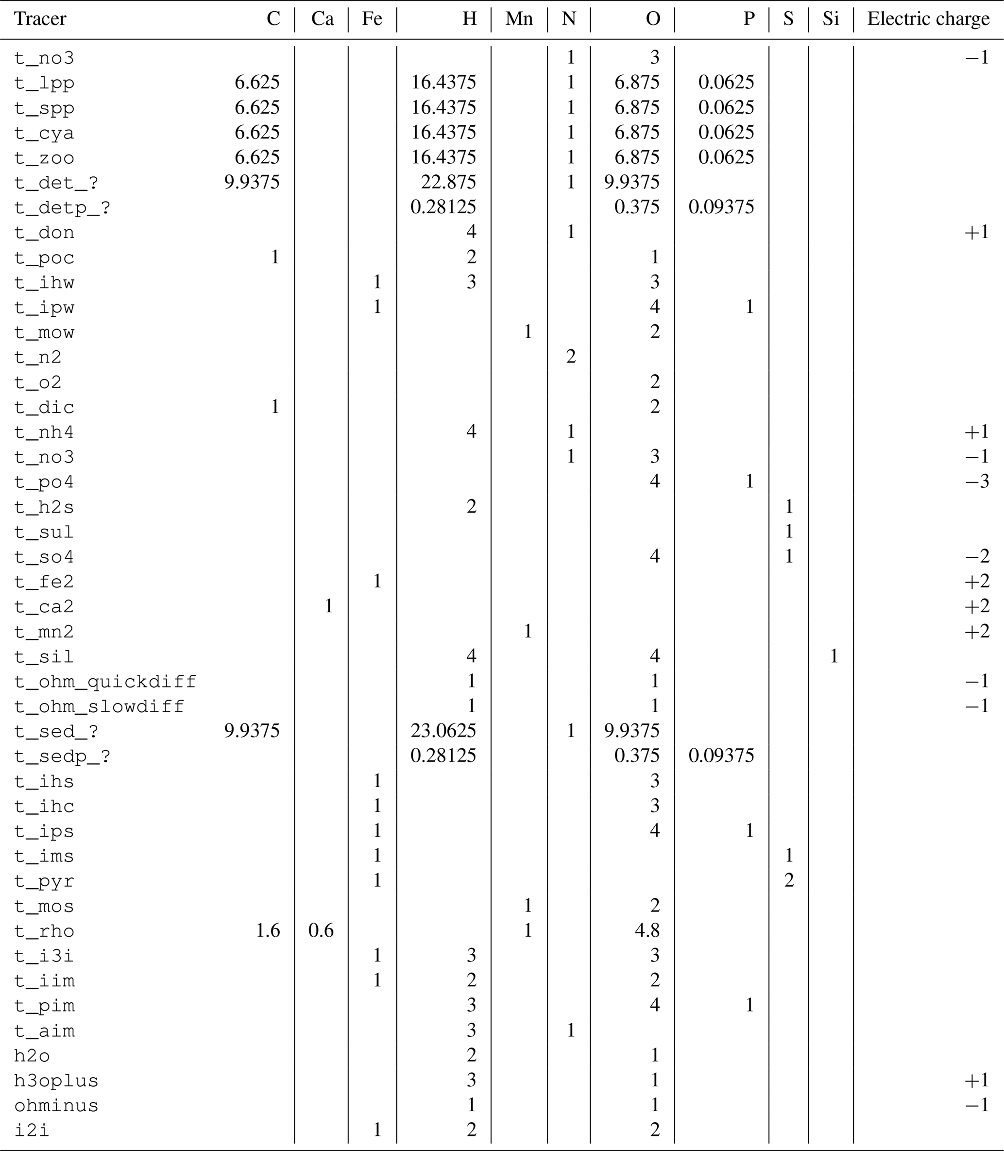
Tracer t_alk has been omitted since it just accumulates
the changes to other tracers.
The study by Middelburg (1989) relates the decay rates of organic carbon to the time since the organic material was deposited. They found the following relation to be valid across timescales from days to decades:
where k denotes the reactivity of organic carbon and t is the time since detritus was created. In our model, we try to resemble this relation by splitting the detritus into different reactivity classes. The ratios rk of the different classes k in freshly created detritus and their reactivities at 0 ∘C are listed in Table B1.
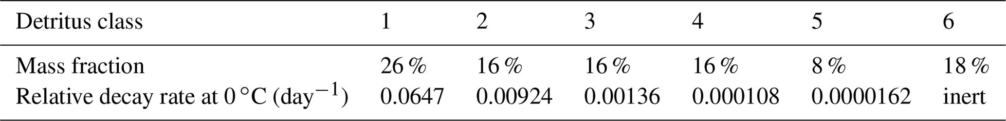
We assume a faster detritus mineralisation at higher temperatures. This is controlled by a factor exp(T⋅τ), which we multiply with the decay rates, where T is the temperature measured in ∘C and τ=0.15 K−1 is a temperature sensitivity constant as it was used in previous versions of the ERGOM model (Neumann and Schernewski, 2008). The effective decay rate of a quantity of fresh detritus changes over time, since the ratio between the detritus classes k changes as the quickly decaying fractions are removed faster. In Fig. B1, we illustrate the effective decay rates predicted by our model at different temperatures and compare them to the rates predicted by the Middelburg formula. We can see that (a) the class model gives a good match to the formula and (b) temperature has little influence on the overall decay rate. The latter fact can be understood as already explained in the main text: a higher temperature means a higher decomposition rate of each detritus class. This will be compensated for in the sum by a shift in the class composition. Lower concentrations of quickly degradable detritus classes will remain, which compensates for the faster decay of the less degradable classes. This means an overall very similar total decomposition rate.
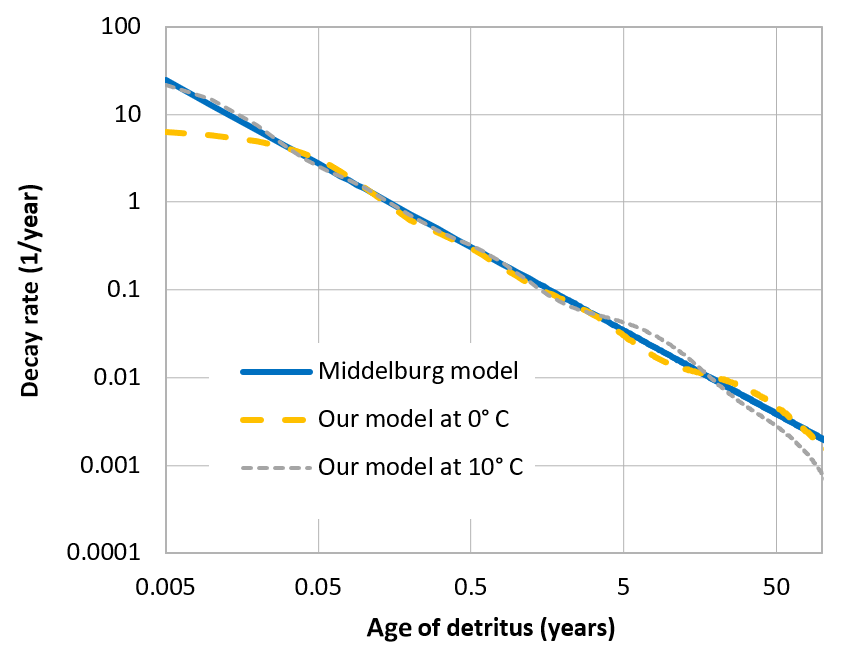
Figure B1Decay rates of organic carbon in detritus depending on its time of creation. Comparison of the reactivity predicted by our model at different temperatures to the Middelburg decay rate prediction; see text.
Here, we use a set of sensitivity experiments to illustrate how the model refinements introduced by us influence the results. In each of these, we switch off one of our model improvements. This means that we use three simplified model versions, in which
-
total alkalinity always diffuses with the bicarbonate diffusivity no matter how many hydroxide ions contribute to it, which in reality diffuse faster,
-
the saturation indices for precipitation–dissolution reactions are calculated neglecting the (salinity-dependent) activity coefficients, and
-
the adsorption of ammonium, phosphate and iron onto clay minerals, as well as their reducible Fe (III) content, is neglected.
As an example, we apply these reduced models to the silt station TW. (Please note that the calibration procedure was not repeated after the model modifications, but the model parameters were left unchanged.)
The results are shown in Fig. C1 as dashed lines and compared to the full model. All modifications affect the dissolved concentrations of iron in different directions. This is probably because both pore water pH and the activity coefficients influence the precipitation to iron monosulfide. The second modification (neglecting activity coefficients) reduces the phosphate concentrations in the pore water. All other pore water species remain virtually unchanged by our model modifications.

Figure C1Pore water concentrations of several dissolved species at the silt station Tromper Wiek. Points and horizontal lines indicate the range of measurements. Solid curves and shading present the model results and indicate year-average concentrations and the seasonal range. Dashed curves show the same, but for a model version which neglects one of our improvements: (a) without correcting the diffusivity of total alkalinity for hydroxide ions; (b) without correcting the solute concentrations by activity coefficients; (c) without assuming adsorption to clay minerals.
Figure D1(a) Porosity at the silt station Tromper Wiek as assumed in the model (solid line) and a porosity profile for a realistic model set-up derived from the April 2014 cruise (dashed line). (b) Pore water concentrations of several dissolved species at the silt station Tromper Wiek. Points and horizontal lines indicate the range of measurements. Solid curves and shading present the original model results and indicate year-average concentrations and the seasonal range. Dashed curves show the same, but for a model version with the realistic porosity profile.
We used vertically constant porosity in our application of the model. Here, we illustrate the effect of this simplification by comparison to a model with a realistic porosity profile; see Fig. D1. A porosity profile was measured at station Tromper Wiek during the April 2014 cruise (Lipka, 2018) and interpolated to the model depths. Below approx. 3 cm of depth, where porosity is decreased in the realistic profile, we see enhanced pore water concentrations for the nutrients and for sulfide. This was to be expected because of the higher ratio between solid material and pore water volume. In contrast, iron concentrations are reduced in higher depths, while manganese concentrations remain constant. While we do not observe qualitatively different behaviour, the differences between the simplified and realistic porosity model are significant, which means the model might benefit from using realistic porosity profiles.
In Fig. E1, we show the pore water profiles at the site Tromper Wiek simulated with the original and with double resolution in the sediments. For numerical stability reasons, a time step for the vertical diffusion of oxygen had to be reduced in the high-resolution run. Apart from that, the runs were identical. It can be seen that most of the vertical profiles look practically identical among the set-ups. For iron, phosphate and sulfide, we can see deviations which we considered as acceptable if we keep the overall uncertainties in mind.
Figure E1Pore water concentrations of several dissolved species at the silt station Tromper Wiek. Points and horizontal lines indicate the range of measurements. Solid curves and shading present the model results and indicate year-average concentrations and the seasonal range. Dashed curves show the same, but for a model version with double vertical resolution.
For solutes, we assume that the flux (positive upward) between two neighbouring cells takes the form
where D is the effective diffusivity calculated as the sum of molecular diffusivity and bioirrigation diffusivity (see Eq. 5), ck denotes the concentration in the pore water of cell k [mol kg−1] and is the distance between the centres of the adjacent cells. This flux means a concentration change in the different grid cells given by
This allows us to construct a matrix MB which transforms the vector of concentrations to its derivative, which is
So, after a time step of Δt, the concentration vector cnew can be determined as
The matrix exponentiation can be defined as
We approximate the limit by choosing s and use the method of Al-Hassan (2012) to compute cnew. This method allows for an efficient calculation of powers of tridiagonal matrices with positive entries, and it is easy to see that is of this shape if n is chosen large enough.
An identical approach is used for the solids.
The supplement related to this article is available online at: https://doi.org/10.5194/gmd-12-275-2019-supplement.
HR developed the model and performed the simulations. ML, DB, CM and JW carried out the experimental work and obtained the data which went into model calibration and validation. MEB, SF, TL, GR and BC contributed to the interpretation of the results and the structuring and formulation of the article. TN was the work package supervisor and developer of the pelagic ecosystem model.
The authors declare that they have no conflict of interest.
This study is embedded in the KÜNO project SECOS (03F0666A) funded by the
German Federal Ministry for Education and Research (BMBF). The model
optimisation runs were performed on the HLRN supercomputing facilities. Free
software which supported this work includes R, R Studio and Free Pascal Lazarus.
Marko Lipka and Michael E. Böttcher wish to thank Iris Schmiedinger, Anne Köhler and Iris Scherff for their invaluable help in the laboratory. They
also wish to express their gratitude to Bo Liu for helpful discussions on
transport processes. Jana Woelfel and Gregor Rehder thank Peter Linke and
Stefan Sommer for the long-lasting loan and technical support (Sergiy Cherednichenko) of the two mini benthic
chamber landers (GEOMAR, Kiel,
Germany).
Edited by: Sandra Arndt
Reviewed by: three anonymous referees
Al-Hassan, Q.: On Powers of Tridiagonal Matrices with Nonnegative Entries, J. Appl. Math. Sci., 6, 2357–2368, 2012. a, b
Al-Raei, A. M., Bosselmann, K., Böttcher, M. E., Hespenheide, B., and Tauber, F.: Seasonal dynamics of microbial sulfate reduction in temperate intertidal surface sediments: controls by temperature and organic matter, Ocean Dynam., 59, 351–370, 2009. a
Andersson, A., Haecky, P., and Hagström, Å.: Effect of temperature and light on the growth of micro-nano-and pico-plankton: impact on algal succession, Mar. Biol., 120, 511–520, 1994. a
Arndt, S., Jørgensen, B. B., LaRowe, D. E., Middelburg, J. J., Pancost, R. D., and Regnier, P.: Quantifying the degradation of organic matter in marine sediments: A review and synthesis, Earth-Sci. Rev., 123, 53–86, https://doi.org/10.1016/j.earscirev.2013.02.008, 2013. a
Bale, A. J. and Morris, A. W.: Organic carbon in suspended particulate material in the North Sea: Effect of mixing resuspended and background particles, Cont. Shelf Res., 18, 1333–1345, https://doi.org/10.1016/S0278-4343(98)00046-6, 1998. a, b
Belmans, F., van Grieken, R., and Brügmann, L.: Geochemical characterization of recent sediments in the Baltic Sea by bulk and electron microprobe analysis, Mar. Chem., 42, 223–236, 1993. a
Berner, R. A.: Early Diagenesis: A Theoretical Approach, Princeton University Press, Princeton, NJ, USA, 1980. a
Boesen, C. and Postma, D.: Pyrite formation in anoxic environments of the Baltic, Am. J. Sci., 288, 575–603, 1988. a
Böttcher, M. E.: Experimental dissolution of CaCO3-MnCO3 solid solutions in CO2-H2O solutions at 20 ∘C: I. Synthetic low-temperature carbonates, Solid State Ionics, 101, 1263–1266, 1997. a
Böttcher, M. E. and Dietzel, M.: Metal-ion partitioning during low-temperature precipitation and dissolution of anhydrous carbonates and sulphates, no. 10 in EMU Notes in Mineralogy, 139–187, Mineralogical Society, https://doi.org/10.1180/EMU-notes.10.4, 2010. a, b
Böttcher, M. E., Hespenheide, B., Llobet-Brossa, E., Beardsley, C., Larsen, O., Schramm, A., Wieland, A., Böttcher, G., Berninger, U.-G., and Amann, R.: The biogeochemistry, stable isotope geochemistry, and microbial community structure of a temperate intertidal mudflat: an integrated study, Cont. Shelf Res., 20, 1749–1769, 2000. a
Boudreau, B. P.: Diagenetic models and their implementation, vol. 505, Springer, Berlin, Germany, 1997. a, b, c, d, e, f, g, h
Boudreau, B. P., Huettel, M., Forster, S., Jahnke, R. A., McLachlan, A., Middelburg, J. J., Nielsen, P., Sansone, F., Taghon, G., and Van Raaphorst, W.: Permeable marine sediments: overturning an old paradigm, EOS, Transactions American Geophysical Union, 82, 133–136, 2001. a, b
Brigolin, D., Lovato, T., Rubino, A., and Pastres, R.: Coupling early-diagenesis and pelagic biogeochemical models for estimating the seasonal variability of N and P fluxes at the sediment–water interface: Application to the northwestern Adriatic coastal zone, J. Marine Syst., 87, 239–255, https://doi.org/10.1016/j.jmarsys.2011.04.006, 2011. a
Bruckner, C. G., Mammitzsch, K., Jost, G., Wendt, J., Labrenz, M., and Jürgens, K.: Chemolithoautotrophic denitrification of epsilonproteobacteria in marine pelagic redox gradients, Environ. Microbiol., 15, 1505–1513, https://doi.org/10.1111/j.1462-2920.2012.02880.x, 2013. a
Bunke, D.: Sediment mixing processes and accumulation patterns in the south-western Baltic Sea, PhD thesis, University of Greifswald (Germany), Greifswald, available at: https://nbn-resolving.org/urn:nbn:de:gbv:9-opus-20780 (last access: 10 January 2019), 2018. a, b
Butenschön, M., Zavatarelli, M., and Vichi, M.: Sensitivity of a marine coupled physical biogeochemical model to time resolution, integration scheme and time splitting method, Ocean Model., 52–53, 36–53, https://doi.org/10.1016/j.ocemod.2012.04.008, 2012. a
Butenschön, M., Clark, J., Aldridge, J. N., Allen, J. I., Artioli, Y., Blackford, J., Bruggeman, J., Cazenave, P., Ciavatta, S., Kay, S., Lessin, G., van Leeuwen, S., van der Molen, J., de Mora, L., Polimene, L., Sailley, S., Stephens, N., and Torres, R.: ERSEM 15.06: a generic model for marine biogeochemistry and the ecosystem dynamics of the lower trophic levels, Geosci. Model Dev., 9, 1293–1339, https://doi.org/10.5194/gmd-9-1293-2016, 2016. a
Cadée, G. C. and Hegeman, J.: Primary production of the benthic microflora living on tidal flats in the Dutch Wadden Sea, Neth. J. Sea Res., 8, 260–291, https://doi.org/10.1016/0077-7579(74)90020-9, 1974. a
Cahill, B., Radtke, H., and Neumann, T.: The role of coastal sediments for water column dynamics in the Western Baltic Sea, in preparation, 2019. a, b
Cahoon, L. B., Nearhoof, J. E., and Tilton, C. L.: Sediment grain size effect on benthic microalgal biomass in shallow aquatic ecosystems, Estuaries, 22, 735–741, 1999. a
Canty, A. and Ripley, B.: boot: Bootstrap Functions (Originally by Angelo Canty for S), available at: https://CRAN.R-project.org/package=boot (last access: 10 January 2019), 2017. a
Capet, A., Meysman, F. J. R., Akoumianaki, I., Soetaert, K., and Grégoire, M.: Integrating sediment biogeochemistry into 3D oceanic models: A study of benthic-pelagic coupling in the Black Sea, Ocean Model., 101, 83–100, https://doi.org/10.1016/j.ocemod.2016.03.006, 2016. a
Cerco, C. F., Noel, M. R., and Kim, S.-C.: Three-dimensional management model for Lake Washington, part II: eutrophication modeling and skill assessment, Lake Reserv. Manage., 22, 115–131, 2006. a
Christiansen, C., Edelvang, K., Emeis, K., Graf, G., Jähmlich, S., Kozuch, J., Laima, M., Leipe, T., Löffler, A., Lund-Hansen, L. C., Miltner, A., Pazdro, K., Pempkowiak, J., Shimmield, G., Shimmield, T., Smith, J., Voss, M., and Witt, G.: Material transport from the nearshore to the basinal environment in the southern Baltic Sea: I. Processes and mass estimates, J. Marine Syst., 35, 133–150, https://doi.org/10.1016/S0924-7963(02)00126-4, 2002. a, b, c, d, e
Cline, J. D.: Spectrophotometric determination of hydrogen sulfide in natural waters, Limnol. Oceanogr., 14, 454–458, 1969. a
Colijn, F. and De Jonge, V. N.: Primary production of microphytobenthos in the Ems-Dollard Estuary, Marine ecology progress series, Oldendorf, Germany, 14, 185–196, 1984. a
Davies, C. W.: The extent of dissociation of salts in water. Part VIII. An equation for the mean ionic activity coefficient of an electrolyte in water, and a revision of the dissociation constants of some sulphates, J. Chem. Soc. (Resumed), 0, 2093–2098, https://doi.org/10.1039/JR9380002093, 1938. a
Davison, A. C. and Hinkley, D. V.: Bootstrap Methods and Their Application, Cambridge University Press, Cambridge, UK, 1997. a
Deutsch, B., Forster, S., Wilhelm, M., Dippner, J. W., and Voss, M.: Denitrification in sediments as a major nitrogen sink in the Baltic Sea: an extrapolation using sediment characteristics, Biogeosciences, 7, 3259–3271, https://doi.org/10.5194/bg-7-3259-2010, 2010. a
Dickson, A. G. and Goyet, C.: Handbook of methods for the analysis of the various parameters of the carbon dioxide system in sea water, Version 2, Tech. rep., Oak Ridge National Lab., TN, USA, 1994. a
Dickson, A. G., Sabine, C. L., and Christian, J. R.: Guide to best practices for ocean CO2 measurements, Tech. Rep. PICES Special Publication 3, PICES, Victoria, Canada, 2007. a, b, c, d, e
Drobner, E., Huber, H., Wächtershäuser, G., Rose, D., and Stetter, K. O.: Pyrite formation linked with hydrogen evolution under anaerobic conditions, Nature, 346, 742–744, 1990. a
Edzwald, J. K., Toensing, D. C., and Leung, M. C.-Y.: Phosphate adsorption reactions with clay minerals, Environ. Sci. Technol., 10, 485–490, 1976. a, b
Emeis, K.-C., Struck, U., Leipe, T., Pollehne, F., Kunzendorf, H., and Christiansen, C.: Changes in the C, N, P burial rates in some Baltic Sea sediments over the last 150 years–relevance to P regeneration rates and the phosphorus cycle, Mar. Geol., 167, 43–59, 2000. a
Emeis, K.-C., Christiansen, C., Edelvang, K., Jähmlich, S., Kozuch, J., Laima, M., Leipe, T., Loeffler, A., Lund-Hansen, L.-C., Miltner, A., Pazdro, K., Pempkowiak, J., Pollehne, F., Shimmield, T., Voss, M., and Witt, G.: Material transport from the near shore to the basinal environment in the southern Baltic Sea: II: synthesis of data on origin and properties of material, J. Marine Syst., 35, 151–168, 2002. a, b, c, d
Engel, A.: Direct relationship between CO2 uptake and transparent exopolymer particles production in natural phytoplankton, J. Plankton Res., 24, 49–53, https://doi.org/10.1093/plankt/24.1.49, 2002. a
Gadani, D. H., Rana, V. A., Bhatnagar, S. P., Prajapati, A. N., and Vyas, A. D.: Effect of salinity on the dielectric properties of water, Indian J. Pure Ap. Phy., 50, 405–410, 2012. a
Gili, J.-M. and Coma, R.: Benthic suspension feeders: their paramount role in littoral marine food webs, Trends Ecol. Evol., 13, 316–321, 1998. a
Glud, R. N.: Oxygen dynamics of marine sediments, Mar. Biol. Res., 4, 243–289, https://doi.org/10.1080/17451000801888726, 2008. a
Glud, R. N., Woelfel, J., Karsten, U., Kühl, M., and Rysgaard, S.: Benthic microalgal production in the Arctic: applied methods and status of the current database, Bot. Mar., 52, 559–571, 2009. a
Gogina, M., Morys, C., Forster, S., Gräwe, U., Friedland, R., and Zettler, M. L.: Towards benthic ecosystem functioning maps: Quantifying bioturbation potential in the German part of the Baltic Sea, Ecol. Indic., 73, 574–588, https://doi.org/10.1016/j.ecolind.2016.10.025, 2017. a
Graf, G. and Rosenberg, R.: Bioresuspension and biodeposition: a review, J. Marine Syst., 11, 269–278, 1997. a
Grasshoff, K., Kremling, K., and Ehrhardt, M.: Methods of seawater analysis, John Wiley & Sons, Weinheim, Germany, 2009. a
Griffies, S.: Fundamentals of ocean climate models, Princeton university press, Princeton, New Jersey, USA, 2018. a
Guisasola, A., Jubany, I., Baeza, J. A., Carrera, J., and Lafuente, J.: Respirometric estimation of the oxygen affinity constants for biological ammonium and nitrite oxidation, J. Chem. Technol. Biot., 80, 388–396, https://doi.org/10.1002/jctb.1202, 2005. a
Gundersen, J. K. and Jorgensen, B. B.: Microstructure of diffusive boundary layers and the oxygen uptake of the sea floor, Nature, 345, 604–607, 1990. a
Haines-Young, R. and Potschin, M.: Common International Classification of Ecosystem Services (CICES): Consultation on Version 4, August–December 2012, Tech. rep., University of Nottingham, available at: https://cices.eu/content/uploads/sites/8/2012/07/CICES-V43_Revised-Final_Report_29012013.pdf (last access: 10 January 2019), 2013. a
Hamme, R. C. and Emerson, S. R.: The solubility of neon, nitrogen and argon in distilled water and seawater, Deep-Sea Res. Pt. I, 51, 1517–1528, 2004. a
Hansen, M. H., Ingvorsen, K., and Jøgensen, B. B.: Mechanisms of hydrogen sulfide release from coastal marine sediments to the atmosphere, Limnol. Oceanogr., 23, 68–76, https://doi.org/10.4319/lo.1978.23.1.0068, 1978. a
Heiskanen, A.-S. and Leppänen, J.-M.: Estimation of export production in the coastal Baltic Sea: effect of resuspension and microbial decomposition on sedimentation measurements, Hydrobiologia, 316, 211–224, 1995. a
HELCOM: Part A. Introductory Chapters, in: Guidelines for the Baltic Monitoring Programme for the Third Stage, no. 27A in Baltic Sea Environment Proceedings, Baltic Marine Environment Protection Commission – Helsinki Commission, Helsinki, Finland, 1988. a
Hooke, R. and Jeeves, T. A.: “Direct Search” Solution of Numerical and Statistical Problems, J. ACM, 8, 212–229, 1961. a
Huber, P. J.: Robust statistics, Wiley series in probability and mathematical statistics, Wiley, New York, USA, 1981. a
Ingall, E. and Jahnke, R.: Influence of water-column anoxia on the elemental fractionation of carbon and phosphorus during sediment diagenesis, Mar. Geol., 139, 219–229, 1997. a
IOW: IOWDB – the oceanographic database of IOW, available at: https://www.io-warnemuende.de/iowdb.html (last access: 10 January 2019), 2017. a
Jaisi, D. P., Dong, H., and Liu, C.: Influence of biogenic Fe (II) on the extent of microbial reduction of Fe (III) in clay minerals nontronite, illite, and chlorite, Geochim. Cosmochim. Ac., 71, 1145–1158, 2007. a, b, c, d
Jakobsen, R. and Postma, D.: Formation and solid solution behavior of Ca-rhodochrosites in marine muds of the Baltic deeps, Geochim. Cosmochim. Ac., 53, 2639–2648, https://doi.org/10.1016/0016-7037(89)90135-X, 1989. a, b, c
Jilbert, T., Slomp, C. P., Gustafsson, B. G., and Boer, W.: Beyond the Fe-P-redox connection: preferential regeneration of phosphorus from organic matter as a key control on Baltic Sea nutrient cycles, Biogeosciences, 8, 1699–1720, https://doi.org/10.5194/bg-8-1699-2011, 2011. a
Jonsson, P., Carman, R., and Wulff, F.: Laminated sediments in the Baltic: a tool for evaluating nutrient mass balances, Ambio, 19, 152–158, 1990. a
Jørgensen, B. B.: Bacteria and Marine Biogeochemistry, in: Marine Geochemistry, edited by: Schulz, H. D. and Zabel, M., Springer-Verlag, Berlin/Heidelberg, 169–206, https://doi.org/10.1007/3-540-32144-6_5, 2006. a
Kalka, H.: Activity Coefficients (Activity Models), available at: http://www.aqion.de/site/101#fn:lg (last access: 10 January 2019), 2018. a
Kersten, M., Leipe, T., and Tauber, F.: Storm disturbance of sediment contaminants at a Hot-Spot in the Baltic Sea assessed by 234Th radionuclide tracer profiles, Environm. Sci. Technol., 39, 984–990, 2005. a
Kowalski, N., Dellwig, O., Beck, M., Grunwald, M., Dürselen, C.-D., Badewien, T. H., Brumsack, H.-J., van Beusekom, J. E., and Böttcher, M. E.: A comparative study of manganese dynamics in the water column and sediments of intertidal systems of the North Sea, Estuar. Coast. Shelf S., 100, 3–17, https://doi.org/10.1016/j.ecss.2011.03.011, 2012. a
Kristensen, E., Ahmed, S. I., and Devol, A. H.: Aerobic and anaerobic decomposition of organic matter in marine sediment: which is fastest?, Limnol. Oceanogr., 40, 1430–1437, 1995. a
Kulik, D. A., Kersten, M., Heiser, U., and Neumann, T.: Application of Gibbs Energy Minimization to Model Early-Diagenetic Solid-Solution Aqueous-Solution Equilibria Involving Authigenic Rhodochrosites in Anoxic Baltic Sea Sediments, Aquat. Geochem., 6, 147–199, 2000. a
Kuliński, K., Schneider, B., Hammer, K., Machulik, U., and Schulz-Bull, D.: The influence of dissolved organic matter on the acid–base system of the Baltic Sea, J. Marine Syst., 132, 106–115, 2014. a
Lancelot, C., Spitz, Y., Gypens, N., Ruddick, K., Becquevort, S., Rousseau, V., Lacroix, G., and Billen, G.: Modelling diatom and Phaeocystis blooms and nutrient cycles in the Southern Bight of the North Sea: the MIRO model, Mar. Ecol. Prog. Ser., 289, 63–78, 2005. a
Large, W. G., McWilliams, J. C., and Doney, S. C.: Oceanic vertical mixing: A review and a model with a nonlocal boundary layer parameterization, Rev. Geophys., 32, 363–403, 1994. a
Lee, J.-Y., Tett, P., Jones, K., Jones, S., Luyten, P., Smith, C., and Wild-Allen, K.: The PROWQM physical–biological model with benthic–pelagic coupling applied to the northern North Sea, J. Sea Res., 48, 287–331, https://doi.org/10.1016/S1385-1101(02)00182-X, 2002. a, b
Leipe, T., Tauber, F., Vallius, H., Virtasalo, J., Uścinowicz, S., Kowalski, N., Hille, S., Lindgren, S., and Myllyvirta, T.: Particulate organic carbon (POC) in surface sediments of the Baltic Sea, Geo.-Mar. Lett., 31, 175–188, 2011. a, b
Leppäranta, M. and Myrberg, K.: Physical oceanography of the Baltic Sea, Springer Science & Business Media, Berlin/Heidelberg, Germany, https://doi.org/10.1007/978-3-662-04453-7, 2009. a
Levinton, J. S.: Marine Biology: Function, Biodiversity, Ecology, 4 edn., Oxford University Press, New York, USA, 2013. a
Lijklema, L.: Interaction of orthophosphate with iron (III) and aluminum hydroxides, Environ. Sci. Technol., 14, 537–541, 1980. a, b
Lipka, M.: Current biogeochemical processes and element fluxes in surface sediments of temperate marginal seas (Baltic Sea and Black Sea), PhD thesis, University of Greifswald, Greifswald, Germany, 2018. a, b, c, d, e, f, g
Lipka, M., Woelfel, J., Gogina, M., Kallmeyer, J., Liu, B., Morys, C., Forster, S., and Böttcher, M. E.: Solute Reservoirs Reflect Variability of Early Diagenetic Processes in Temperate Brackish Surface Sediments, Frontiers in Marine Science, 5, 413, https://doi.org/10.3389/fmars.2018.00413, 2018a. a, b
Lipka, M., Wölfel, J., Gogina, M., Liu, B., and Böttcher, M. E.: Spatiotemporal dynamics in solute reservoirs of temperate brackish surface sediments, Annual Report 2017, Leibniz Institute for Baltic Sea Research Warnemuende (IOW), Warnemuende, available at: https://www.io-warnemuende.de/tl_files/forschung/pdf/IOW-Jahresbericht-2017.pdf (last access: 10 January 2019), 2018b. a
Llobet-Brossa, E.: Microbial Community Composition of Wadden Sea Sediments as Revealed by Fluorescence In Situ Hybridization, Appl. Environ. Microbiol., 64, 2691–2696, 1998. a
Luff, R. and Moll, A.: Seasonal dynamics of the North Sea sediments using a three-dimensional coupled sediment–water model system, Cont. Shelf Res., 24, 1099–1127, 2004. a
Maar, M., Møller, E. F., Larsen, J., Madsen, K. S., Wan, Z., She, J., Jonasson, L., and Neumann, T.: Ecosystem modelling across a salinity gradient from the North Sea to the Baltic Sea, Ecol. Model., 222, 1696–1711, https://doi.org/10.1016/j.ecolmodel.2011.03.006, 2011. a
Marcus, N. H.: Minireview: The importance of benthic-pelagic coupling and the forgotten role of life cycles in coastal aquatic systems, Limnol. Oceanogr., 43, 763–768, 1998. a
Meire, L., Soetaert, K. E. R., and Meysman, F. J. R.: Impact of global change on coastal oxygen dynamics and risk of hypoxia, Biogeosciences, 10, 2633–2653, https://doi.org/10.5194/bg-10-2633-2013, 2013. a
Meysman, F. J., Galaktionov, O. S., Gribsholt, B., and Middelburg, J. J.: Bioirrigation in permeable sediments: Advective pore-water transport induced by burrow ventilation, Limnol. Oceanogr., 51, 142–156, 2006. a
Meysman, F. J., Malyuga, V. S., Boudreau, B. P., and Middelburg, J. J.: A generalized stochastic approach to particle dispersal in soils and sediments, Geochim. Cosmochim. Ac., 72, 3460–3478, https://doi.org/10.1016/j.gca.2008.04.023, 2008. a
Middelburg, J. J.: A simple rate model for organic matter decomposition in marine sediments, Geochim. Cosmochim. Ac., 53, 1577–1581, 1989. a, b, c
Millero, F. J.: Thermodynamics of the carbon dioxide system in the oceans, Geochim. Cosmochim. Ac., 59, 661–677, https://doi.org/10.1016/0016-7037(94)00354-O, 1995. a
Millero, F. J. and Leung, W. H.: The thermodynamics of seawater at one atmosphere, Am. J. Sci., 276, 1035–1077, https://doi.org/10.2475/ajs.276.9.1035, 1976. a
Millero, F. J., Sotolongo, S., and Izaguirre, M.: The oxidation kinetics of Fe(II) in seawater, Geochim. Cosmochim. Ac., 51, 793–801, https://doi.org/10.1016/0016-7037(87)90093-7, 1987. a
Moberg, E. G. and Harding, M. W.: The Boron Content of Sea Water, Science, 77, 510–510, https://doi.org/10.1126/science.77.2004.510, 1933. a
Morse, J. W., Millero, F. J., Cornwell, J. C., and Rickard, D.: The chemistry of the hydrogen sulfide and iron sulfide systems in natural waters, Earth-Sci. Rev., 24, 1–42, https://doi.org/10.1016/0012-8252(87)90046-8, 1987. a, b
Morys, C.: Particle dynamics in sediments of the western Baltic Sea, PhD thesis, University of Rostock, Rostock, Germany, available at: http://rosdok.uni-rostock.de/file/rosdok_disshab_0000001661/rosdok_derivate_0000035932/Dissertation_Morys_2017.pdf (last access: 10 January 2019), 2016. a, b
Morys, C.: Seasonality of bioturbation – what governs the intensity of local and non-local sediment mixing?, in preparation, 2019. a
Morys, C., Forster, S., and Graf, G.: Variability of bioturbation in various sediment types and on different spatial scales in the southwestern Baltic Sea, Mar. Ecol. Prog. Ser., 557, 31–49, https://doi.org/10.3354/meps11837, 2016. a, b, c
Morys, C., Powilleit, M., and Forster, S.: Bioturbation in relation to the depth distribution of macrozoobenthos in the southwestern Baltic Sea, Mar. Ecol. Prog. Ser., 579, 19–36, https://doi.org/10.3354/meps12236, 2017. a
Neumann, T.: Towards a 3D-ecosystem model of the Baltic Sea, J. Marine Syst., 25, 405–419, https://doi.org/10.1016/S0924-7963(00)00030-0, 2000. a
Neumann, T. and Schernewski, G.: Eutrophication in the Baltic Sea and shifts in nitrogen fixation analyzed with a 3D ecosystem model, J. Marine Syst., 74, 592–602, 2008. a, b, c
Neumann, T., Siegel, H., and Gerth, M.: A new radiation model for Baltic Sea ecosystem modelling, J. Marine Syst., 152, 83–91, https://doi.org/10.1016/j.jmarsys.2015.08.001, 2015. a, b
Neumann, T., Radtke, H., and Seifert, T.: On the importance of Major Baltic Inflows for oxygenation of the central Baltic Sea, J. Geophys. Res.-Oceans, 122, 1090–1101, 2017. a, b, c, d, e, f, g
Oliveros-Ramos, R. and Shin, Y.-J.: Calibrar: an R package for fitting complex ecological models, arXiv preprint arXiv:1603.03141, available at: https://arxiv.org/abs/1603.03141, (last access: 10 January 2019), 2016. a
Osipov, V. I.: Density of clay minerals, Soil Mech. Found. Eng., 48, 231–240, 2012. a
Paraska, D. W., Hipsey, M. R., and Salmon, S. U.: Sediment diagenesis models: Review of approaches, challenges and opportunities, Environ. Modell. Softw., 61, 297–325, https://doi.org/10.1016/j.envsoft.2014.05.011, 2014. a
Pinckney, J. and Zingmark, R. G.: Biomass and production of benthic microalgal communities in estuarine habitats, Estuaries, 16, 887–897, 1993. a
Raaphorst, W. V. and Malschaert, J. F. P.: Ammonium adsorption in superficial North Sea sediments, Cont. Shelf Res., 16, 1415–1435, https://doi.org/10.1016/0278-4343(95)00081-X, 1996. a, b
Radtke, H.: ERGOM-SED-1D, Zenodo, https://doi.org/10.5281/zenodo.2480056, 2018. a
Radtke, H. and Burchard, H.: A positive and multi-element conserving time stepping scheme for biogeochemical processes in marine ecosystem models, Ocean Model., 85, 32–41, 2015. a, b, c
Radtke, H., Neumann, T., Voss, M., and Fennel, W.: Modeling pathways of riverine nitrogen and phosphorus in the Baltic Sea, J. Geophys. Res., 117, C09024, https://doi.org/10.1029/2012JC008119, 2012. a, b
Reed, D. C., Slomp, C. P., and Gustafssonb, B. G.: Sedimentary phosphorus dynamics and the evolution of bottom-water hypoxia: A coupled benthic–pelagic model of a coastal system, Limnol. Oceanogr, 56, 1075–1092, 2011. a, b, c, d, e, f, g, h, i
Rickard, D.: Kinetics of pyrite formation by the H2S oxidation of iron (II) monosulfide in aqueous solutions between 25 and 125 C: The rate equation, Geochim. Cosmochim. Ac., 61, 115–134, 1997. a
Rickard, D. and Luther, G. W.: Kinetics of pyrite formation by the H2S oxidation of iron (II) monosulfide in aqueous solutions between 25 and 125 C: The mechanism, Geochim. Cosmochim. Ac., 61, 135–147, 1997. a, b
Rickard, D. and Luther, G. W.: Chemistry of Iron Sulfides, Chem. Rev., 107, 514–562, https://doi.org/10.1021/cr0503658, 2007. a
Rudstam, L. G., Aneer, G., and Hildén, M.: Top-down control in the pelagic Baltic ecosystem, Dana, 10, 105–129, 1994. a
Rusch, A., Forster, S., and Huettel, M.: Bacteria, diatoms and detritus in an intertidal sandflat subject to advective transport across the water-sediment interface, Biogeochemistry, 55, 1–27, 2001. a
Sarazin, G., Michard, G., and Prevot, F.: A rapid and accurate spectroscopic method for alkalinity measurements in sea water samples, Water Res., 33, 290–294, 1999. a
Sawicka, J. E., Jørgensen, B. B., and Brüchert, V.: Temperature characteristics of bacterial sulfate reduction in continental shelf and slope sediments, Biogeosciences, 9, 3425–3435, https://doi.org/10.5194/bg-9-3425-2012, 2012. a
Schippers, A. and Jørgensen, B. B.: Biogeochemistry of pyrite and iron sulfide oxidation in marine sediments, Geochim. Cosmochim. Ac., 66, 85–92, 2002. a
Schmidt, M. and Eggert, A.: Oxygen cycling in the northern Benguela Upwelling System: Modelling oxygen sources and sinks, Prog. Oceanogr., 149, 145–173, 2016. a
Schneider, B., Nausch, G., and Pohl, C.: Mineralization of organic matter and nitrogen transformations in the Gotland Sea deep water, Mar. Chem., 119, 153–161, https://doi.org/10.1016/j.marchem.2010.02.004, 2010. a
Schulz, J.-P. and Schattler, U.: Kurze Beschreibung des Lokal-Modells Europa COSMO-EU (LME) und seiner Datenbanken auf dem Datenserver des DWD, Tech. rep., German Weather Service, available at: prefixhttps://www.dwd.de/SharedDocs/downloads/DE/modelldokumentationen/nwv/cosmo_eu/cosmo_eu_dbbeschr_201406.pdf (last access: 10 January 2019), 2014. a
Seitzinger, S. P., Nixon, S. W., and Pilson, M. E.: Denitrification and nitrous oxide production in a coastal marine ecosystem, Limnol. Oceanogr., 29, 73–83, 1984. a
Soetaert, K. and Middelburg, J. J.: Modeling eutrophication and oligotrophication of shallow-water marine systems: the importance of sediments under stratified and well-mixed conditions, in: Eutrophication in Coastal Ecosystems, 239–254, Springer, Dordrecht, the Netherlands, 2009. a
Soetaert, K., Herman, P. M., and Middelburg, J. J.: A model of early diagenetic processes from the shelf to abyssal depths, Geochim. Cosmochim. Ac., 60, 1019–1040, 1996a. a
Soetaert, K., Herman, P. M., Middelburg, J. J., Heip, C., deStigter, H. S., van Weering, T. C., Epping, E., and Helder, W.: Modeling 210Pb-derived mixing activity in ocean margin sediments: diffusive versus nonlocal mixing, J. Mar. Res., 54, 1207–1227, 1996b. a, b, c
Soetaert, K., Herman, P. M., Middelburg, J. J., Heip, C., Smith, C. L., Tett, P., and Wild-Allen, K.: Numerical modelling of the shelf break ecosystem: reproducing benthic and pelagic measurements, Deep-Sea Res. Pt. II, 48, 3141–3177, 2001. a, b
Sohma, A., Sekiguchi, Y., Kuwae, T., and Nakamura, Y.: A benthic–pelagic coupled ecosystem model to estimate the hypoxic estuary including tidal flat – Model description and validation of seasonal/daily dynamics, Ecol. Model., 215, 10–39, https://doi.org/10.1016/j.ecolmodel.2008.02.027, 2008. a
Sohma, A., Shibuki, H., Nakajima, F., Kubo, A., and Kuwae, T.: Modeling a coastal ecosystem to estimate climate change mitigation and a model demonstration in Tokyo Bay, Ecol. Model., 384, 261–289, 2018. a
Stephenson, M. and Stickland, L. H.: Hydrogenase: The reduction of sulphate to sulphide by molecular hydrogen, Biochem. J., 25, 215–220, 1931. a
Struck, U., Pollehne, F., Bauerfeind, E., and v. Bodungen, B.: Sources of nitrogen for the vertical particle flux in the Gotland Sea (Baltic Proper) – results from sediment trap studies, J. Marine Syst., 45, 91–101, https://doi.org/10.1016/j.jmarsys.2003.11.012, 2004. a
Stumm, W. and Morgan, J. J.: Aquatic chemistry: chemical equilibria and rates in natural waters, vol. 126, John Wiley & Sons, Hoboken, New Jersey, USA, 2012. a
Sun, M., Aller, R. C., and Lee, C.: Early diagenesis of chlorophyll-a in Long Island Sound sediments: A measure of carbon flux and particle reworking, J. Mar. Res., 49, 379–401, 1991. a
Sunagawa, I.: Nucleation, Growth And Dissolution Of Crystals During Sedimentogenesis and Diagenesis, chap. 2, in: Developments in Sedimentology, edited by: Wolf, K. H. and Chilingarian, G. V., vol. 51 of Diagenesis, IV, 19–47, Elsevier, https://doi.org/10.1016/S0070-4571(08)70435-7,1994. a
Sundby, B., Gobeil, C., Silverberg, N., and Mucci, A.: The phosphorus cycle in coastal marine sediments, Limnol. Oceanogr, 37, 1129–1145, 1992. a, b
Tauber, F.: Online-Karte: Sedimentverteilung auf dem Meeresboden, available at: https://www.geoseaportal.de/mapapps/resources/apps/sedimentverteilung_auf_dem_meeresboden/index.html?lang=de (last access: 10 January 2019), 2012. a
Thamdrup, B., Hansen, J. W., and Jørgensen, B. B.: Temperature dependence of aerobic respiration in a coastal sediment, FEMS Microbiol. Ecol., 25, 189–200, https://doi.org/10.1111/j.1574-6941.1998.tb00472.x, 1998. a
Theberge, S. M. and Iii, G. W. L.: Determination of the Electrochemical Properties of a Soluble Aqueous FeS Species Present in Sulfidic Solutions, Aquat. Geochem., 3, 191–211, https://doi.org/10.1023/A:1009648026806, 1997. a
Turekian, K. K.: Oceans, Prentice-Hall, Upper Saddle River, New Jersey, USA, 1968. a
Ulfsbo, A., Kuliński, K., Anderson, L. G., and Turner, D. R.: Modelling organic alkalinity in the Baltic Sea using a Humic-Pitzer approach, Mar. Chem., 168, 18–26, 2015. a
Uppala, S. M., Kållberg, P. W., Simmons, A. J., Andrae, U., Bechtold, V. d., Fiorino, M., Gibson, J. K., Haseler, J., Hernandez, A., and Kelly, G. A.: The ERA-40 re-analysis, Q. J. Roy. Meteor. Soc., 131, 2961–3012, 2005. a
van Cappellen, P. and Wang, Y.: Cycling of iron and manganese in surface sediments; a general theory for the coupled transport and reaction of carbon, oxygen, nitrogen, sulfur, iron, and manganese, Am. J. Sci., 296, 197–243, https://doi.org/10.2475/ajs.296.3.197, 1996. a, b, c, d
van de Bund, W. J., Ólafsson, E., Modig, H., and Elmgren, R.: Effects of the coexisting Baltic amphipods Monoporeia affinis and Pontoporeia femorata on the fate of a simulated spring diatom bloom, Mar. Ecol. Prog. Ser., 212, 107–115, 2001. a
Venables, W. N. and Ripley, B. D.: Modern Applied Statistics with S, Springer, New York, USA, 2002. a
Voss, M. and Struck, U.: Stable nitrogen and carbon isotopes as indicator of eutrophication of the Oder river (Baltic Sea), Mar. Chem., 59, 35–49, 1997. a
Wasmund, N.: Occurrence of cyanobacterial blooms in the Baltic Sea in relation to environmental conditions, Int. Rev. Hydrobiol., 82, 169–184, 1997. a
Weisse, R., von Storch, H., Callies, U., Chrastansky, A., Feser, F., Grabemann, I., Guenther, H., Plüss, A., Stoye, T., and Tellkamp, J.: Regional meteorological–marine Reanalyses and climate change projections: Results for Northern Europe and potential for coastal and offshore applications, B. Am. Meteorol. Soc., 90, 849–860, 2009. a
Werner, U., Billerbeck, M., Polerecky, L., Franke, U., Huettel, M., Van Beusekom, J. E., and De Beer, D.: Spatial and temporal patterns of mineralization rates and oxygen distribution in a permeable intertidal sand flat (Sylt, Germany), Limnol. Oceanogr., 51, 2549–2563, 2006. a
Westrich, J. T. and Berner, R. A.: The role of sedimentary organic matter in bacterial sulfate reduction: the G model tested, Limnol. Oceanogr., 29, 236–249, 1984. a
Wijsman, J. W. M., Herman, P. M. J., Middelburg, J. J., and Soetaert, K.: A Model for Early Diagenetic Processes in Sediments of the Continental Shelf of the Black Sea, Estuar. Coast. Shelf S., 54, 403–421, https://doi.org/10.1006/ecss.2000.0655, 2002. a, b
Winde, V., Böttcher, M., Escher, P., Böning, P., Beck, M., Liebezeit, G., and Schneider, B.: Tidal and spatial variations of DI13C and aquatic chemistry in a temperate tidal basin during winter time, J. Marine Syst., 129, 396–404, https://doi.org/10.1016/j.jmarsys.2013.08.005, 2014. a
Winkler, L. W.: Die Bestimmung des im Wasser gelösten Sauerstoffes, Ber. Dtsch. Chem. Ges., 21, 2843–2854, https://doi.org/10.1002/cber.188802102122, 1888. a
Yakushev, E. V., Protsenko, E. A., Bruggeman, J., Wallhead, P., Pakhomova, S. V., Yakubov, S. Kh., Bellerby, R. G. J., and Couture, R.-M.: Bottom RedOx Model (BROM v.1.1): a coupled benthic–pelagic model for simulation of water and sediment biogeochemistry, Geosci. Model Dev., 10, 453–482, https://doi.org/10.5194/gmd-10-453-2017, 2017. a
physics/temperature.txt, physics/salinity.txt, physics/light_at_top.txt, physics/bottom_stress.txt, physics/diffusivity.txt, found in the subdirectories
stations/station_?? in the Supplement.
physics/cellheights.txt, physics/sed_cellheights.txt
physics/sed_inert_ratio.txt
physics/diffusivity.txt
While bioturbation in reality causes both a transport of solids and solutes, we use the term “bioturbation” in the model to describe the transport of solids only, while the transport of solutes is done by the “bioirrigation” process.
physics/sed_diffusivity_solids.txt
physics/sed_depth_bioturbation.txt
physics/sed_diffusivity_porewater.txt
physics/sed_inert_deposition.txt
physics/diffusivity.txt
physics/sed_inert_deposition.txt
Throughout the paper, we use the term “detritus” in its biological meaning; here, it describes dead particulate organic material only, as opposed to its use in geology, where the term includes deposited mineral particles.
Middelburg's equation states that material which is decomposed later will be decomposed slower. This may be because the material itself is different or because the oxidant is different. The Middelburg model includes both effects, and splitting them in a mechanistic model would mean preferring one theory or the other. So what we do assume if we just apply the Middelburg model is that the time which a particle spends in the oxic zone, the anoxic zone and the sulfidic zone is similar in our setting to Middelburg's experiments. In this case, the Middelburg model will include the correct slowing-down of degradation caused by the less efficient oxidant.
https://www.mathworks.com/matlabcentral/fileexchange/26294-calculated-dielectric-constant-of-sea-water/content/dielec.m, last access: 10 January 2019
This term differs per variable, but is the same at each station and sampling depth.
- Abstract
- Introduction
- Model description
- Observed data used for model applications
- Model set-up and optimisation
- Model results and validation
- Conclusions
- Code and data availability
- Appendix A: Stoichiometric composition of model state variables
- Appendix B: Rates of organic carbon mineralisation
- Appendix C: Quantitative influence of different model extensions
- Appendix D: Sensitivity analysis for vertically varying porosity
- Appendix E: Sensitivity analysis for vertical resolution in the sediments
- Appendix F: Numerical details of applying the Al-Hassan method
- Author contributions
- Competing interests
- Acknowledgements
- References
- Supplement