the Creative Commons Attribution 4.0 License.
the Creative Commons Attribution 4.0 License.
 | 10 Jul 2019
Weather and climate forecasting with neural networks: using general circulation models (GCMs) with different complexity as a study ground
Sebastian Scher
Gabriele Messori
Recently, there has been growing interest in the possibility of using neural networks for both weather forecasting and the generation of climate datasets. We use a bottom–up approach for assessing whether it should, in principle, be possible to do this. We use the relatively simple general circulation models (GCMs) PUMA and PLASIM as a simplified reality on which we train deep neural networks, which we then use for predicting the model weather at lead times of a few days. We specifically assess how the complexity of the climate model affects the neural network's forecast skill and how dependent the skill is on the length of the provided training period. Additionally, we show that using the neural networks to reproduce the climate of general circulation models including a seasonal cycle remains challenging – in contrast to earlier promising results on a model without seasonal cycle.
- Article
(3099 KB) -
Supplement
(33872 KB) - BibTeX
- EndNote


Synoptic weather forecasting (forecasting the weather at lead times of a few days up to 2 weeks) has for decades been dominated by computer models based on physical equations – the so-called numerical weather prediction (NWP) models. The quality of NWP forecasts has been steadily increasing since their inception (Bauer et al., 2015), and these models remain the backbone of virtually all weather forecasts. However, the fundamental nature of the weather forecasting problem can be summarized as follows: starting from today's state of the atmosphere, we want to predict the state of the atmosphere x days in the future. Thus posed, the problem is a good candidate for supervised machine learning. While this was long thought unfeasible, the recent success of machine learning techniques in highly complex fields such as image and speech recognition warrants a review of this possibility. Machine learning techniques have already been used to improve certain components of NWP and climate models – mainly parameterization schemes (Krasnopolsky and Fox-Rabinovitz, 2006; Rasp et al., 2018; Krasnopolsky et al., 2013; O'Gorman and Dwyer, 2018), to aid real-time decision making (McGovern et al., 2017) to exploit observations and targeted high-resolution simulations to enhance earth system models (Schneider et al., 2017), for El Niño predictions (Nooteboom et al., 2018), and to predict weather forecast uncertainty (Scher and Messori, 2018).
Recently, in addition to using machine learning to enhance numerical models, there have been ambitions to use it to tackle weather forecasting itself. The holy grail is to use machine learning, and especially “deep learning”, to completely replace NWP models, although opinions may diverge on if and when this will happen. Additionally, it is an appealing idea to use neural networks or deep learning to emulate very expensive general circulation models (GCMs) for climate research. Both these ideas have been tested with some success for simplified realities (Dueben and Bauer, 2018; Scher, 2018). In Scher (2018), a neural network approach was used to skillfully forecast the “weather” of a simplified climate model, as well as emulate its climate. Dueben and Bauer (2018), based on their success in forecasting reanalysis data regridded to very low resolution, concluded that it is “fundamentally” possible to produce deep-learning based weather forecasts.
Here, we build upon the approach from Scher (2018) and apply it to a range of climate models with different complexity. We do this in order to assess (1) how the skill of the neural network weather forecasts depends on the available amount of training data; (2) how this skill depends on the complexity of the climate models; and (3) under which conditions it may be possible to make stable climate simulations with the trained networks and how this depends on the amount of available training data. Question (1) is of special interest for the idea of using historical observations in order to train a neural network for weather forecasting. As the length of historical observations is strongly constrained (∼100 years for long reanalyses assimilating only surface observations and ∼40 years for reanalyses assimilating satellite data), it is crucial to assess how many years of past data one would need in order to produce meaningful forecasts. The value of (2) lies in evaluating the feasibility of climate models as a “simplified reality” for studying weather forecasting with neural networks. Finally, (3) is of interest when one wants to use neural networks not only for weather forecasting, but for the distinct yet related problem of seasonal and longer forecasts up to climate projections.
To avoid confusion, we use the following naming conventions throughout the paper: “model” always refers to physical models (i.e., the climate models used in this study) and will never refer to a “machine learning model”. The neural networks are referred to by the term “network”.
2.1 Climate models
To create long climate model runs of different complexity, we used the Planet Simulator (PLASIM) intermediate-complexity GCM, and its dry dynamical core: the Portable University Model of the Atmosphere (PUMA) (Fraedrich et al., 2005). Each model was run for 830 years with two different horizontal resolutions (T21 and T42, corresponding to ∼5.65 and ∼2.8∘ latitude, respectively) and 10 vertical levels. The first 30 years of each run were discarded as spin-up, leaving 800 years of daily data for each model. The runs will from now on be referred to as plasimt21, plasimt42, pumat21 and pumat42. All the model runs produce a stable climate without drift (Figs. S1–S10 in the Supplement). Additionally, we regridded plasimt42 and pumat42 (with bilinear interpolation) to a resolution of T21. These will be referred to as plasimt42_regridT21 and pumat42_regridT21.
The PUMA runs do not include ocean and orography and use Newtonian cooling for diabatic heating or cooling. The PLASIM runs include orography, but no ocean model. The main difference between PLASIM and standard GCMs is that sub-systems of the Earth system other than the atmosphere (e.g., the ocean, sea ice and soil) are reduced to systems of low complexity. We used the default integration time step for all four model setups, namely 30 min for plasimt42, 20 min for plasimt21, and 60 min for pumat21 and pumat42. We regrid all fields to regular lat–long grids on pressure levels for analysis. An additional run was made with PUMA at resolution T21, but with the seasonal cycle switched off (eternal boreal winter). This is the same configuration as used in Scher (2018) and will be referred to as pumat21_noseas.
In order to contextualize our results relative to previous studies, we also run a brief trial of our networks on ERA5 (C3S, 2017) reanalysis data (Sect. 3.5), similar to Dueben and Bauer (2018).
2.2 Complexity
Ranking climate models according to their “complexity” is a nontrivial task, as it is very hard to define what complexity actually means in this context. We note that here we use the term loosely and do not refer to any of the very precise definitions of complexity that exist in various scientific fields (e.g., Johnson, 2009). Intuitively, one might simply rank the models according to their horizontal and vertical resolutions and the number of physical processes they include. However, it is not clear which effects would be more important (e.g., is a model with higher resolution but less components or processes more or less complex than a low-resolution model with a larger number of processes?). Additionally, more physical processes do not necessarily imply a more complex output. For example, very simple models like the Lorenz63 model (Lorenz, 1963) display chaotic behavior, yet it is certainly possible to design a model with more parameters and a deterministic behavior.
To circumvent this conundrum, we adopt a very pragmatic approach based solely on the output of the models and grounded in dynamical systems theory. We quantify model complexity in terms of the local dimension d: a measure of the number of degrees of freedom of a system active locally around a given instantaneous state. In our case, this means that we can compute a value of d for every time step in a given model simulation. While not a measure of complexity in the strict mathematical or computational senses of the term, d provides an objective indication of a system's dynamics around a given state and, when averaged over a long time series, of the system's average attractor dimension. An example of how d may be computed for climate fields is provided in Faranda et al. (2017), while for a more formal discussion and derivation of d, we point the reader to Appendix A in Faranda et al. (2019). The approach is very flexible and may be applied to individual variables of a system (which represent projections of the full phase-space dynamics onto specific subspaces, called Poincaré sections), multiple variables or, with adequate computational resources, to the whole available dataset. The exact algorithm used here is outlined in Appendix A.
The local dimension was computed for 38 years of each model run, as well as for the ERA-Interim reanalysis on a grid over 1979–2016 (Dee et al., 2011). The choice of 38 years was made because this is the amount of available years in ERA-Interim, and the length of the data series can affect the estimate of d (Buschow and Friederichs, 2018). Figure 1 shows the results for 500 hPa geopotential height. The complexity of PUMA increases with increasing resolution, whereas both the low- and the high-resolution PLASIM model have a complexity approaching that of ERA-Interim. Thus – at least by this measure – they are comparable to the real atmosphere. The high-resolution runs regridded to T21 have nearly the same complexity as the original high-resolution runs. The ranking is the same for nearly all variables and levels (Fig. S11). For the rest of the paper, the term complexity or “complex” always refers to the local dimension d.
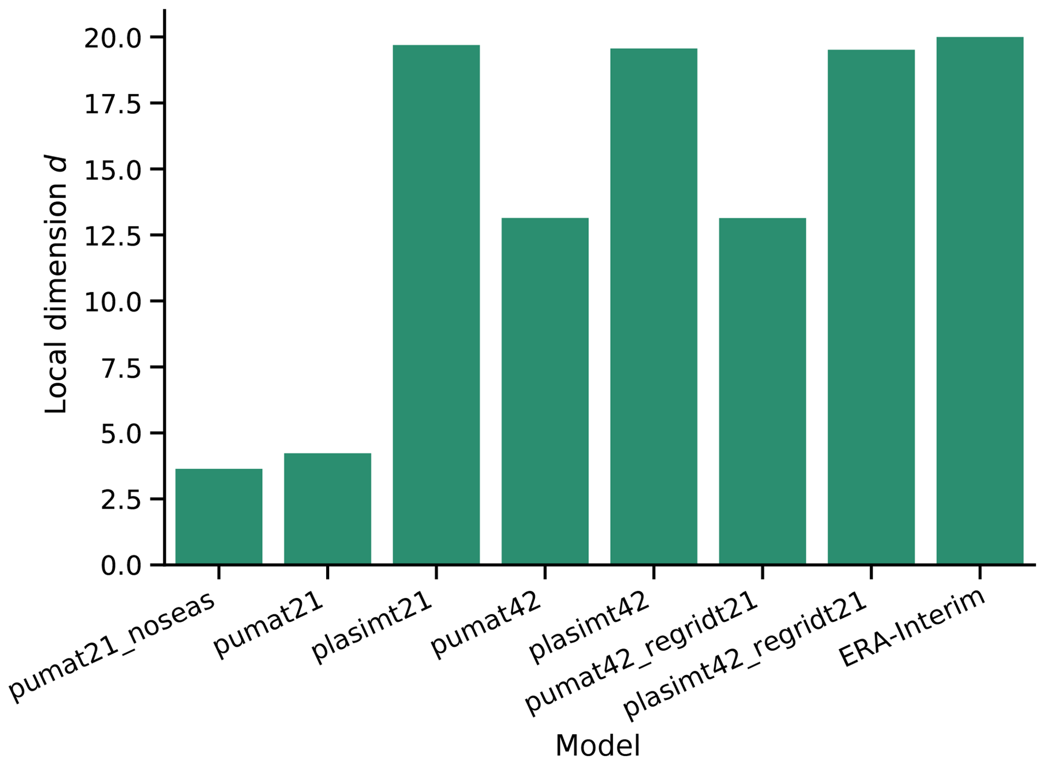
Figure 1Averages of the local dimension d (here used as a data-based measure of complexity) for the 500 hPa geopotential height of the models used in this study and of the ERA-Interim reanalysis.
2.3 Neural networks
Neural networks are in principle a series of nonlinear functions with weights determined through training on data. Before the training, one has to decide the architecture of the network. Here, we use the architecture proposed by Scher (2018), which is a convolutional decoder–encoder, taking as input 3-D model fields and outputting 3-D model fields of exactly the same dimension. It was designed and tuned in order to work well on pumat21 without seasonality (for details, see Scher, 2018). In order to ease comparison with previous results, in the main part of this study we use the same network layout and hyperparameters as in Scher (2018), except for the number of epochs (iterations over the training set) the network is trained over. In the original configuration only 10 epochs were used. It turned out that, especially for the more complex models, the training was not saturated after 10 epochs. Therefore, here we train until the skill of the validation data has not increased for 5 epochs, with a maximum of 100 epochs. The layout is depicted in Fig. 2. The possibility of retuning the network and its implications are discussed in Sect. 3.4. For the networks targeted to create climate simulations (hereafter called climate networks), we deviate from this setup: here, we include the day of year as additional input to the network, in the form of a separate input channel. To remain consistent with the encoder–decoder setup, the output also contains the layer with the day of year. However, when producing the network climate runs, the predicted day of the year is discarded.
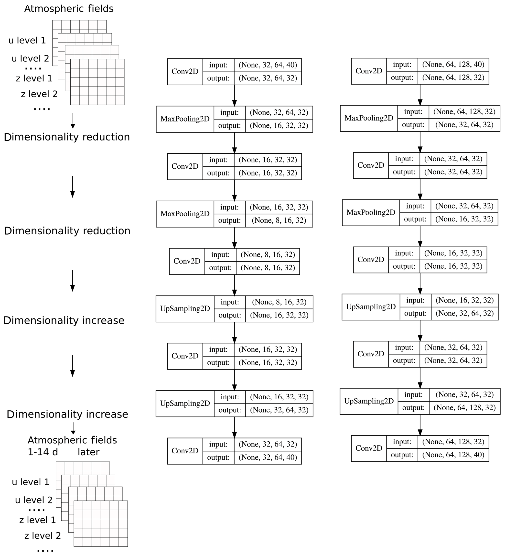
Figure 2Architecture of the neural network for the models with resolution T21 (left) and T42 (right). Each box describes a network layer, with the numbers indicating the dimension of (None, lat, long, level). “None” refers to the time dimension that is not relevant here but which we include in the schematic since it is part of the basic notation of the software library used. Figure based on Fig. S1 from Scher (2018).
The last 10 % samples of the training data are used for validation. This allows us to monitor the training progress, control overfitting (the situation where the network works very well on the training data, but very poorly on the test data) and potentially limit the maximum number of training epochs. As input to the neural networks we use four variables (u, v, t and z) at 10 pressure levels; each variable at each level is represented as a separate input layer (channel). These four variables represent the full state of the PUMA model. PLASIM has three additional atmospheric variables related to the hydrological cycle (relative humidity, cloud liquid water content and cloud cover). In order to keep the architecture the same, these are not included in the standard training and only used for a test in Sect. 3.5.
All networks are trained to make 1 d (1 day) forecasts. Longer forecasts are made by iteratively feeding back the forecast into the network. We did not train the network directly on longer lead times, based on the finding of Dueben and Bauer (2018) that it is easier to make multiple short forecasts compared to a single long one. Due to the availability of model data and in keeping with Scher (2018), we chose 1 d forecasts as opposed to the shorter forecast step (1 h) in Dueben and Bauer (2018). For each model, the network was trained with a set of 1, 2, 5, 10, 20, 50, 100, 200, 400 and 800 years. Since with little training data the network is less constrained, and the training success might strongly depend on exactly which short period out of the model run is chosen, the training for periods up to and including 20 years was repeated four times, shifting the start of the training data by 10, 20, 30 and 40 years. The impact of the exact choice of training period is discussed where appropriate. All the analyses shown in this paper are performed on the forecasts made on the first 30 years of the model run, which were never used during training and therefore provide objective scores (the “test” dataset).
2.4 Metrics
All network forecasts are validated against the underlying model the network was trained on (e.g., for the forecasts of the network trained on plasimt21, the “truth” is the evolution of the plasimt21 run). We specifically adopt two widely used forecast verification metrics, namely the root mean square error (RMSE) and the anomaly correlation coefficient (ACC). The RMSE is defined as
where the overbar denotes a mean over space and time (for global measures) or over time only (for single grid points). The ACC measures the spatial correlation of the forecast anomaly fields with the true anomaly fields for a single forecast. The anomalies are computed with respect to a 30 d running climatology, computed on 30 years of model data (similar to how the European Centre for Medium Range Weather Forecasts computes its scores for forecast validation).
To compute a score over the whole period, the ACCs for all individual forecasts are simply averaged:
The ACC ranges from −1 to 1, with 1 indicating a perfect correlation of the anomaly fields and 0 no correlation at all.
For the evaluation of the brief ERA5 test in Sect. 3.6, we use the mean absolute error instead of RMSE to keep in line with Dueben and Bauer (2018). The mean absolute error is defined as
3.1 Forecast skill in a hierarchy of models
We start by analyzing the RMSE and ACC of two of the most important variables: 500 hPa geopotential height (hereafter zg500) and 800 hPa temperature (hereafter ta800). The first is one of the most commonly used validation metrics in NWP; the second is very close to temperature at 850 hPa, which is another commonly used validation metric. We focus on the networks trained with 100 years of training data, which is the same length as in Scher (2018) and is of special interest because it is roughly the same length as is available in current century-long reanalyses like ERA-20C and the NCEP/NCAR 20CR (Compo et al., 2011; Poli et al., 2016). Figure 3 shows the global mean RMSE of network forecasts at lead times of up to 14 d for all models for both zg500 and ta800. Additionally, the skill of persistence forecasts (using the initial state as forecast) is shown with dashed lines. As expected, the skill of the network forecasts decreases monotonically with lead time. Unsurprisingly, the network for pumat21_noseas – the least complex model – has the highest skill (lowest error) for all lead times for both variables, followed by the network for pumat21. The network for pumat42, which is more complex than pumat21 but less complex than the two PLASIM runs, lies in between. At a lead time of 1 d, the networks for both PLASIM runs have very similar skill, but the plasimt42 network has higher errors at longer lead times, despite their very similar complexity. Here we have to note that at long lead times and near-zero ACC, RMSE can be hard to interpret since it can be strongly influenced by biases in the forecasts. When looking at the ACC instead (higher values better), the picture is very similar. The network forecasts outperform the persistence baseline (dashed lines) at nearly all lead times, except for the plasimt21 and plasimt42 cases, where the RMSE of the network forecasts is higher from around 9 d onwards (depending on the variable). The periodic behavior of the persistence forecast skill for PUMA is caused by eastwards traveling Rossby waves, whose structure is relatively simple in the PUMA model. For the T42 runs that were regridded to T21 before the training the results are as follows: for PUMA, the skill of the network in predicting the regridded version of the T42 is very similar to the skill on the original T42 run. For PLASIM the skill of the regridded T42 run is comparable to both the skill of T42 and of T21 runs, albeit closer to the latter. Indeed, the skills of the original PLASIM T42 and T21 runs are much closer to each other than for PUMA. Regridding the network predictions of the two T42 runs to the T21 grid thus results in only very small changes relative to the difference between the models, especially at longer lead times (not shown).
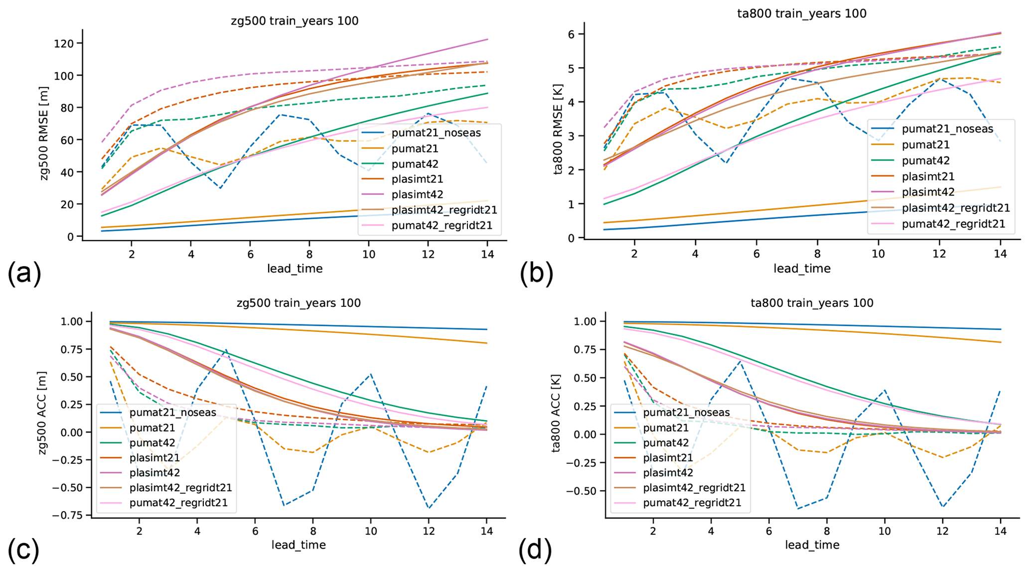
Figure 3Root mean square error (RMSE) and anomaly correlation coefficient (ACC) of 500 hPa geopotential height (a, c) and 800 hPa temperature (b, d) for network forecasts (solid lines) and persistence forecasts (dashed lines) for all models for different lead times (in days). All forecasts are based on 100 years of training data.
We next turn our attention to the spatial characteristics of the forecast error. Figure 4 shows geographical plots of the RMSE for 6 d forecasts of the networks trained with 100 years of data (the same training length as in Fig. 3). In agreement with the global mean RMSE analyzed before, the network for pumat21_noseas has the lowest errors everywhere (Fig. S12), followed by the network for pumat21. The networks for plasimt21 and plasimt42 have a more complicated spatial error structure, and the midlatitude storm tracks emerge clearly as high-error regions. The zonally nonuniform distribution is likely caused by the influence of orography (present in the PLASIM runs but not in the PUMA runs). At lead time 1 d, the errors of the network forecasts for pumat42 are nearly symmetric (not shown), but at longer lead times a zonal asymmetry emerges (Fig. 4b). This is probably related to the fact that the neural network used here does not wrap around the boundaries.
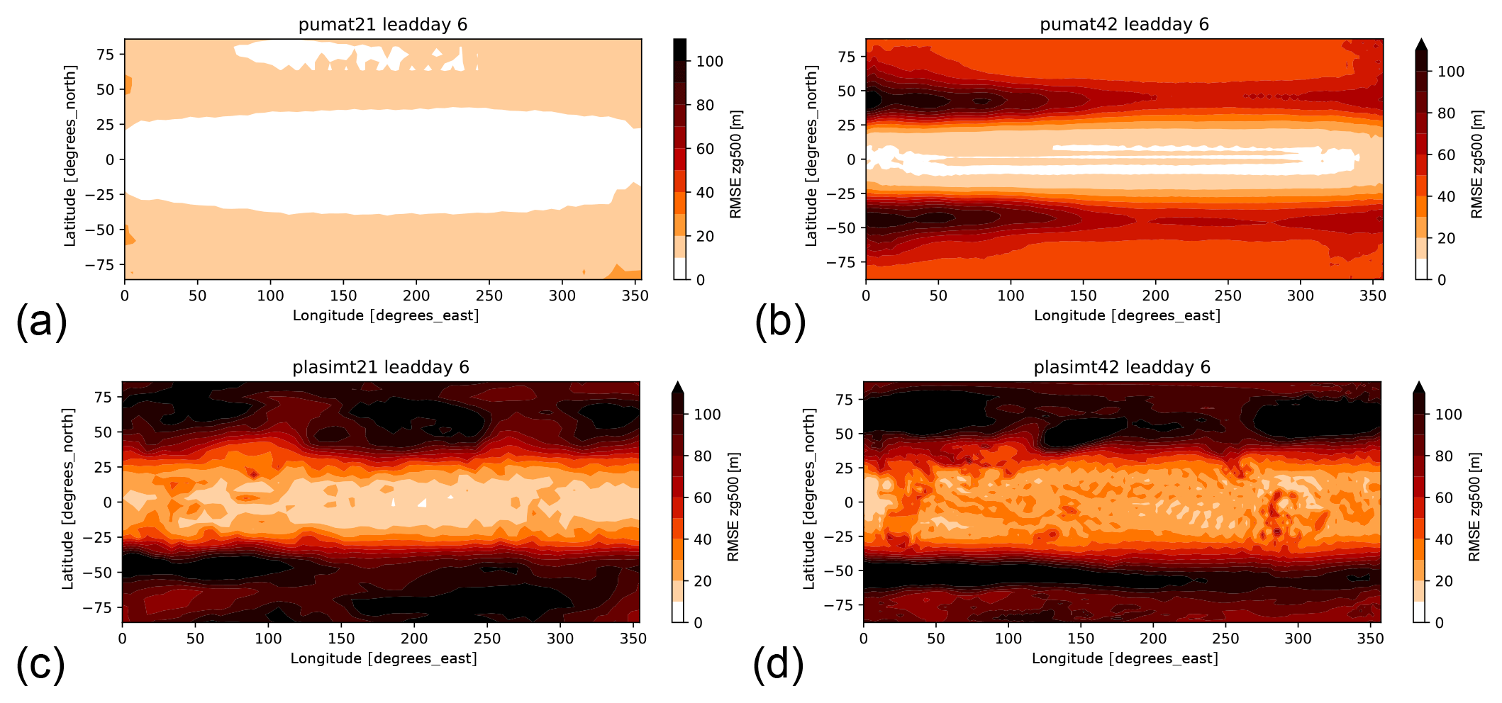
Figure 4Maps of RMSE of the 6 d network forecasts, for the networks trained with 100 years for pumat21 (a), pumat42 (b), plasimt21 (c) and plasimt42 (d).
3.2 Dependence of forecast skill on the amount of training years
A key issue is the extent to which the above results, and more generally the skill of the network forecasts, depend on the length of the training period used. Figure 5 shows the skill of the network forecasts for 500 hPa geopotential height for different training lengths, for a lead time of 1 d (a, c) and 6 d (b, d). As mentioned in the Methods section, the networks with short training periods were trained several times with different samples from the model runs. The shading in the figure represents the uncertainty of the mean for these multi-sample networks, which is negligibly small. For the 1 d forecasts (Fig. 5a, c), the results are as expected: the skill increases with an increasing number of training years, both in terms of RMSE and ACC. This increase is strongly nonlinear, and, beyond ∼100 years, the skill benefit of increasing the length of the training set is limited. This suggests that the complete model space is already encompassed by around 100 years of daily data. More years will not provide new information to the network. However, it might also be the case that there is in fact more information in more years but that the network is not able to utilize this additional information effectively. For the 6 d forecasts (Fig. 5b, d), the plasimt21 networks display a counterintuitive behavior: the skill (in terms of RMSE) does not increase monotonically with increasing length of the training period, but decreases from 100 to 200 years, while for >200 years it increases again. A similar result – albeit less pronounced – is also seen for the plasimt42_regridT21 networks and also – in a slightly different form – for the skill measured via the ACC. To interpret this, one has to remember that the networks are all trained on 1 d forecasts. For 1 d forecasts the skill does indeed increase with increasing training length, and the pumat21 network trained on 200 years makes better forecasts than the one trained on 100 years (Fig. 5a, c). Intuitively one would assume this to translate to increased skill of the consecutive forecasts used to create the 6 d forecasts. The fact that this is not the case here might be caused by nonlinear error growth. Some networks might produce slightly lower errors at lead day 1, but those particular errors could be faster-growing than those of a network with larger day-1 errors.
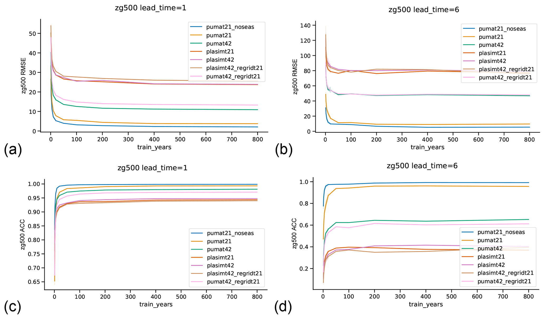
Figure 5Dependence of network forecast skill on the length of the training period. Shown is the root mean square error (RMSE) and anomaly correlation coefficient (ACC) of the network-forecasted 500 hPa geopotential height for networks trained on different amounts of training years. Each line represents one model. The shading on the left side of the plots represents the 5–95 uncertainty range of the mean RMSE or ACC, estimated over networks with different training samples.
3.3 Climate runs with the networks
The trained networks are not limited to forecasting the model weather but can also be used to generate a climate run starting from an arbitrary state of the climate model. For this, we use the climate networks that also include the day of year as input (see Sect. 2). The question of whether the climate time series obtained from the network is stable is of special interest. In Scher (2018), the network climate for pumat21_noseas (using 100 years of training data) was stable and produced reasonable statistics compared to the climate model. We trained our climate networks on both 30 and 100 years of data for all models with seasonal cycle. While the networks were all stable, they do not produce particularly realistic representations of the model climates. After some time, the storm tracks look unrealistic and the seasonal cycle is also poorly represented (e.g., in some years, some seasons are skipped – see Videos S1–S8 in the Supplement that show the evolution of zg500 and zonal wind speed at 300 hPa for the network climate runs). Figure 6a shows the evolution of ta800 at a single grid point at 76∘ N for pumat21 and the climate network trained on 30 years, started from the same (randomly selected) initial state (results for different randomly selected initial states are very similar, not shown). The network is stable, but the variance is too high and some summers are left out. Surprisingly, the network for 30 years of plasimt21 (Fig. 6b) produced a more realistic climate. Training on 100 years instead of 30 years does not necessarily improve the quality of the climate runs (Fig. 6c, d). In fact, for plasimt21 the network climate trained on 100 years is the worse performer. Interestingly, the mean climate of the plasimt21 network is reasonably realistic for the network trained on 100 years (Fig. 7) and partly also for the network trained on 30 years (not shown), whereas the mean climates for the plasimt42 and pumat42 networks have large biases (see Figs. S11–S17).
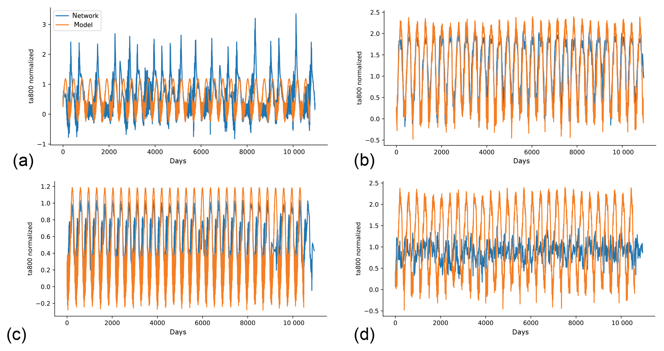
Figure 6Evolution of daily ta800 at a single grid point at 76∘ N in the GCM (orange) and in the climate network trained on the GCM (blue), started from the same initial state. The networks were trained on 30 years of pumat21 (a), 30 years of plasimt21 (b), 100 years of pumat21 (c) and 100 years of plasimt21 (d).
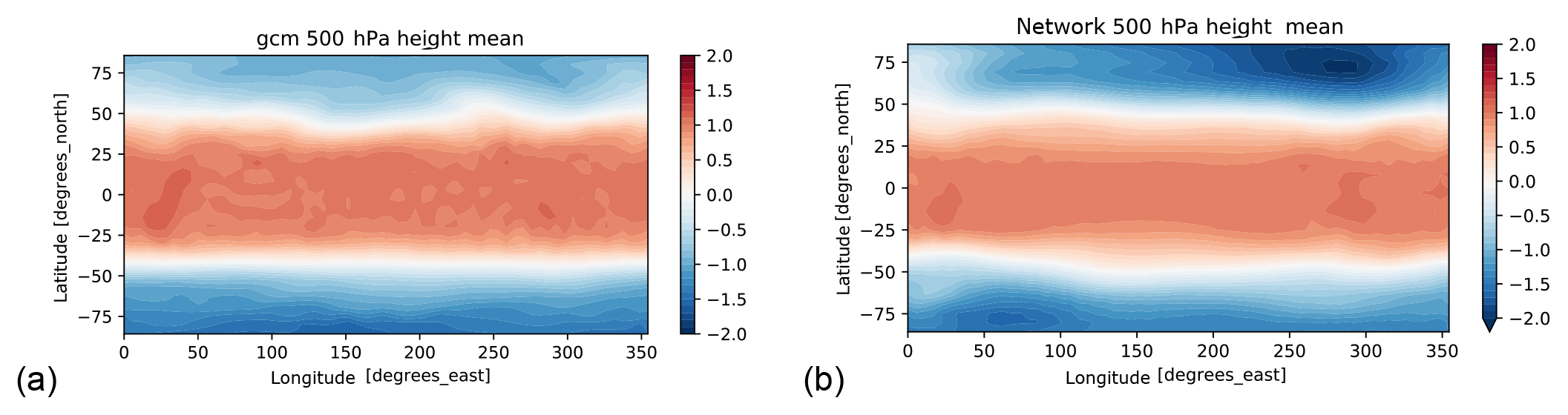
Figure 7Thirty-year mean of normalized 500 hPa geopotential height for plasimt21 (a) and the network trained on 100 years of plasimt21 (b).
All our networks were trained to make 1 d forecasts. The influence of the seasonal cycle on atmospheric dynamics – and especially the influence of diabatic effects – may be very small for 1 d predictions. This could make it hard for the network to learn the influence of seasonality. To test this, we repeated the training of the climate network for plasimt21 but now training on 5 d forecasts. This improved the seasonality of ta800 at our example grid point (Fig. S19), but the spatial fields of the climate run still become unrealistic (Video S9).
3.4 Impact of retuning
The design of this study was to use an already established neural network architecture – namely one tuned on a very simple model – and apply it to more complex models. However, it is of interest to know how much tuning the network architecture to the more complex models might increase forecast skill. Therefore, the same tuning procedure as in Scher (2018) for pumat21_noseas was repeated for plasimt21. Surprisingly, the resulting configuration for plasimt21 was exactly the same as for pumat21_noseas. Thus, even with retuning the results would be the same. As a caveat, we note that tuning neural networks is an intricate process, and many arbitrary choices have to be made. Notably, one has to predefine the different configurations that are tried out in the tuning (the “tuning space”). It is possible that with a different tuning space for plasimt21, a different configuration would be chosen than for pumat21_noseas. However, at least within the tuning space we used, we can conclude that a setup that works well for a very simple model (pumat21_noseas) is also a good choice for a more complex model like plasimt21.
3.5 Impact of including hydrological cycle as input
PLASIM, in contrast to PUMA, includes a hydrological cycle. This is represented by three additional 3-D state variables in the model (relative humidity, cloud liquid water content and cloud cover). To the test the impact of including these variables in the neural networks, we retrained the network for 100 years of plasimt21 including these three variables (on 10 levels) as additional channels both in the input and output of the network. The network thus has 70 instead of 40 in- and output channels. Quite surprisingly, including the hydrological cycle variables slightly deteriorated the forecasts of zg500 and ta800, both in terms of RMSE and ACC, except for the ACC of ta800 from lead times of 6 d onwards (Fig. S20).
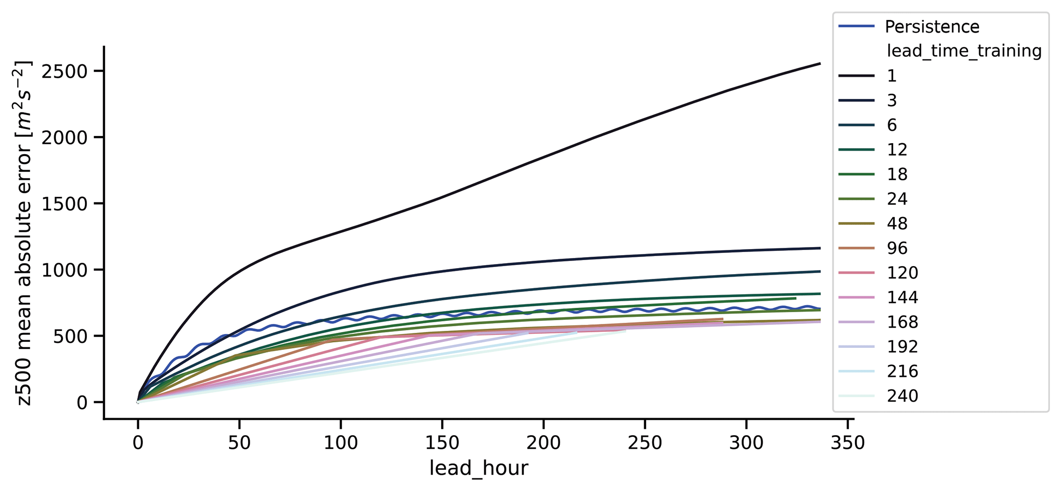
Figure 8Mean absolute error of 500 hPa geopotential height for networks trained on coarse-grained (T21) ERA5 data. The training was performed on different lead times. The x axis denotes the lead time of the forecast in hours and the colors the lead time used for training (in hours). Also shown is the persistence forecast (thick blue line).
3.6 Performance on reanalysis data
In order to put our results into context, we also trained our network architecture on coarse-grained (regridded to T21) ERA5 (C3S, 2017) reanalysis data. We use exactly the same dataset that Dueben and Bauer (2018) used, namely 7 years (2010–2016) for training and 8 months for evaluation (January 2017–August 2017). ERA5 is available at hourly intervals, allowing a thorough investigation of which time step is best for training. As in Dueben and Bauer (2018), we only use zg500 and therefore deviate from the setup used in the rest of this study. We do this in order to be able to directly compare the results in the two studies. We trained networks on lead times ranging from 1 to 240 h, and computed the skill of the zg500 forecasts. The results are shown in Fig. 8. The blue line shows the error of persistence forecasts. The network trained on 1 h forecasts is not stable and has very high forecast errors, in contrast to Dueben and Bauer who only obtained good forecasts with training on a 1 h lead time. The network trained with a 24 h lead time has comparable skill to the network used by Dueben and Bauer (2018) (see their Fig. 3a). For longer lead times, the networks trained on longer lead times seem to work better. In general, it seems that if one wishes to have forecasts for a certain lead time, it is best to train directly on that lead time, at least for mean absolute error.
We have tested the use of neural networks for forecasting the “weather” in a range of simple climate models with different complexity. For this we have used a deep convolutional encoder–decoder architecture that Scher (2018) developed for a very simple general circulation model without seasonal cycle. The network is trained on the model in order to forecast the model state 1 d ahead. This process is then iterated to obtain forecasts at longer lead times. We also performed “climate” runs, where the network is started with a random initial state from the climate model run and then creates a run of daily fields for several decades.
4.1 Potential improvements in the neural network architecture
In the architecture used in this paper, lat–long grids are used to represent the fields. The convolution layers consist of a set of fixed filters that are moved across the domain. Therefore, the same filter is used close to the poles and close to the Equator, even though the area represented by a single grid point is not the same close to the poles and close to the Equator since the Earth is a globe. Using spherical convolution layers as proposed in Coors et al. (2018) would tackle this problem and may lead to improved forecasts and/or more realistic long-term simulations. The tuning of the network architecture used here tuned the depth of the convolution layers but not the actual number of convolution layers. Therefore, it would be interesting to explore whether deeper networks (more convolution layers) could improve the performance of the networks. Other possible improvements would be to
-
include one or more locally connected layers in addition to the convolution layers. While they can increase problems related with overfitting, locally connected layers could learn “local dynamics”.
-
include spatial dependence in height. In our architecture, all variables at all heights are treated as individual channels. One could for example group variables at one height together or use 3d convolution.
Our results further support the idea – already proposed by Dueben and Bauer (2018) and Scher (2018) – of training a neural network on the large amount of existing climate model simulations, feeding the trained network with today's analysis of a NWP model and using the network to make a weather forecast. The high computational efficiency of such neural network forecasts would open up new possibilities, for example of creating ensemble forecasts with much large ensemble sizes than the ones available today. Therefore, this approach would provide an interesting addition to current weather forecasting practice and also a good example of exploiting the large amount of existing climate model data for new purposes.
4.2 Networks for weather forecasts and climate runs
One of the aims of this study was to assess whether it is possible to use a simplified reality – in this case a very simple GCM without seasonal cycle – to develop a method that also works on more complex GCMs. We showed that, for the problem of forecasting the model weather, this seems to be the case: the network architecture developed by Scher (2018) also worked on the more complex models used here, albeit with lower skill. The latter point is hardly surprising, as one would expect the time evolution of the more complex models to be harder to predict. The neural network forecast outperformed a simple persistence forecast baseline at most lead times also for the more complex models. The fact that we can successfully forecast the weather in a range of simple GCMs a couple of days ahead is an encouraging result for the idea of weather forecasting with neural networks. We also tried to retune the network architecture from Scher (2018) to one of our more complex models. Surprisingly, the best network configuration that came out of the tuning procedure was exactly the same as the one obtained for the simpler model in Scher (2018). This further supports the idea that methods developed on simpler models may be fruitfully applied in more complex settings. Additionally, we tested the network architecture on coarse-grained reanalysis data, where its skill is comparable to the method proposed by Dueben and Bauer (2018). We also found that, in contrast to the findings of Dueben and Bauer (2018), it seems possible to make valid neural network forecasts of atmospheric dynamics using a wide range of time steps (also much longer than 1 h). This discrepancy might be caused by our use of convolutional layers, in contrast to the local deep neural network that Dueben and Bauer used. A stack of convolution layers may be interpreted as multiple layers, where each layer could possibly make a short-term forecast and the whole stack a long-term forecast.
The second problem we addressed was using the trained networks to create climate runs. Scher (2018) found this generated a stable climate for the simplest model considered here, which does not have a seasonal cycle. Here, we find that this is to some extent also possible for more complex models. However, even when training on relatively long periods (100 years), the climates produced by the networks have some unrealistic properties, such as a poor seasonal cycle, significant biases in the long-term mean values and often unrealistic storm tracks. The fact that these problems do not occur for the simplest GCM without seasonal cycle but do occur for the same GCM with seasonal cycle indicates that seasonality considerably complicates the problem. While not a solution for creating climate runs, this suggests that for the weather forecasting problem, it might be interesting to train separate networks for different times of the year (e.g., one for each month).
The code developed and used for this study is available in the accompanying repository at https://doi.org/10.5281/zenodo.2572863 (Scher, 2019b). All external libraries used here are open source. The trained networks and the data underlying all the plots are available in the repository. The model runs can be recreated with the control files (available in the repository) and the source code of PUMA/PLASIM, which is freely available at https://www.mi.uni-hamburg.de/en/arbeitsgruppen/theoretische-meteorologie/modelle/PLASIM.html (last access: 8 July 2019.). ERA-Interim data are freely available at https://apps.ecmwf.int/datasets/data/interim-full-daily/levtype=pl/ (last access: 8 July 2019). ERA5 data are freely available at https://climate.copernicus.eu/climate-reanalysis (last access: 8 July 2019).
Here, we outline very briefly how the local dimension d is computed. To foster easy reproducibility, we present the computation in an algorithm-like fashion, as opposed to formal mathematical notation. For a more rigorous theoretical explanation the reader is referred to Faranda et al. (2019). The code is available in the repository accompanying this paper (see “Code and data availability”).
First, we define the distance between the 2-D atmospheric fields at times t1 and t2 as
where j is the linear grid point index and Nj is the total number of grid points. To compute dt, namely the local dimension of a field at time t, we first take the negative natural logarithm of the distances between t and all other time steps ti (i.e., all times before and after t),
and then retain only the distances that are above the 98th percentile of :
These are effectively logarithmic returns in phase space, corresponding to cases where the field is very close to the field xt. According to the Freitas–Freitas–Todd theorem (Freitas et al., 2010), modified in Lucarini et al. (2012), the probability of such logarithmic returns (in the limit of an infinitely long time series) follows the exponential member of the generalized Pareto distribution (Pickands III, 1975). The local dimension dt can then be obtained as the inverse of the distribution's scale parameter, which can also be expressed as the inverse of the mean of the exceedances:
The local dimension is an instantaneous metric, and Faranda et al. (2019) have shown that time averaging of the data can lead to counterintuitive effects. The most robust approach is therefore to compute d on instantaneous fields. Here, in order to use the same data as for the machine learning, we have used daily means. We have verified that, at least in ERA-Interim, this has a negligible effect on the average d value for all variables except for geopotential height at 100 and 200 hPa (not shown).
The videos in the Supplement show the evolution of the GCM (upper panels) and the evolution of the climate network trained on the GCM (lower panels), both started from the same initial conditions. The left panels show zg500, the right panels wind speed at 300 hPa. Each video corresponds to one GCM. The videos can be accessed at https://doi.org/10.5281/zenodo.3248691 (Scher, 2019a).
SS conceived the study and methodology, performed the analysis, produced the software and drafted the article. GM contributed to drafting and revising the article.
The authors declare that they have no conflict of interest.
We thank Peter Dueben for providing the ERA5 data. Sebastian Scher was funded by the Department of Meteorology (MISU) of Stockholm University. The computations were done on resources provided by the Swedish National Infrastructure for Computing (SNIC) at the High Performance Computing Center North (HPC2N) and National Supercomputer Centre (NSC).
This research has been supported by Vetenskapsrådet (grant no. 2016-03724).
This paper was edited by Samuel Remy and reviewed by Peter Düben and two anonymous referees.
Bauer, P., Thorpe, A., and Brunet, G.: The quiet revolution of numerical weather prediction, Nature, 525, 47–55, https://doi.org/10.1038/nature14956, 2015. a
Buschow, S. and Friederichs, P.: Local dimension and recurrent circulation patterns in long-term climate simulations, arXiv preprint arXiv:1803.11255, 2018. a
C3S: ERA5: Fifth generation of ECMWF atmospheric reanalyses of the global climate, Copernicus Climate Change Service Climate Data Store (CDS), available at: https://cds.climate.copernicus.eu/cdsapp#!/home (last access: 7 June 2019), 2017. a, b
Compo, G. P., Whitaker, J. S., Sardeshmukh, P. D., Matsui, N., Allan, R. J., Yin, X., Gleason, B. E., Vose, R. S., Rutledge, G., Bessemoulin, P., Brönnimann, S., Brunet, M., Crouthamel, R. I., Grant, A. N., Groisman, P. Y., Jones, P. D., Kruk, M. C., Kruger, A. C., Marshall, G. J., Maugeri, M., Mok, H. Y., Nordli, Ø., Ross, T. F., Trigo, R. M., Wang, X. L., Woodruff, S. D., and Worley, S. J.: The twentieth century reanalysis project, Q. J. Roy. Meteor. Soc., 137, 1–28, 2011. a
Coors, B., Paul Condurache, A., and Geiger, A.: Spherenet: Learning spherical representations for detection and classification in omnidirectional images, in: Proceedings of the European Conference on Computer Vision (ECCV), September 2018, Munich, Germany, 518–533, 2018. a
Dee, D. P., Uppala, S. M., Simmons, A., Berrisford, P., Poli, P., Kobayashi, S., Andrae, U., Balmaseda, M., Balsamo, G., Bauer, P., Bechtold, P., Beljaars, A. C., van de Berg, L., Bidlot, J., Bormann, N., Delsol, C., Dragani, R., Fuentes, M., Geer, A. J., Haimberger, L., Healy, S. B., Hersbach, H., Hólm, E. V., Isaksen, L., Kållberg, P., Köhler, M., Matricardi, M., McNally, A. P., Monge-Sanz, B. M., Morcrette, J., Park, B., Peubey, C., de Rosnay, P., Tavolato, C., Thépaut, J., and Vitart, F.: The ERA-Interim reanalysis: Configuration and performance of the data assimilation system, Q. J. Roy. Meteor. Soc., 137, 553–597, 2011. a
Dueben, P. D. and Bauer, P.: Challenges and design choices for global weather and climate models based on machine learning, Geosci. Model Dev., 11, 3999–4009, https://doi.org/10.5194/gmd-11-3999-2018, 2018 a, b, c, d, e, f, g, h, i, j, k, l, m
Faranda, D., Messori, G., and Yiou, P.: Dynamical proxies of North Atlantic predictability and extremes, Scientific Reports, 7, 41278, https://doi.org/10.1038/srep41278, 2017. a
Faranda, D., Messori, G., and Vannitsem, S.: Attractor dimension of time-averaged climate observables: insights from a low-order ocean-atmosphere model, Tellus A, 71, 1–11, https://doi.org/10.1080/16000870.2018.1554413, 2019. a, b, c
Fraedrich, K., Jansen, H., Kirk, E., Luksch, U., and Lunkeit, F.: The Planet Simulator: Towards a user friendly model, Meteorol. Z., 14, 299–304, https://doi.org/10.1127/0941-2948/2005/0043, 2005. a
Freitas, A. C. M., Freitas, J. M., and Todd, M.: Hitting time statistics and extreme value theory, Probab. Theory Rel., 147, 675–710, 2010. a
Johnson, N.: Simply complexity: A clear guide to complexity theory, Oneworld Publications, London, UK, 2009. a
Krasnopolsky, V. M. and Fox-Rabinovitz, M. S.: Complex hybrid models combining deterministic and machine learning components for numerical climate modeling and weather prediction, Neural Networks, 19, 122–134, https://doi.org/10.1016/j.neunet.2006.01.002, 2006. a
Krasnopolsky, V. M., Fox-Rabinovitz, M. S., and Belochitski, A. A.: Using ensemble of neural networks to learn stochastic convection parameterizations for climate and numerical weather prediction models from data simulated by a cloud resolving model, Advances in Artificial Neural Systems, 2013, 485913, https://doi.org/10.1155/2013/485913, 2013. a
Lorenz, E. N.: Deterministic nonperiodic flow, J. Atmo. Sci., 20, 130–141, 1963. a
Lucarini, V., Faranda, D., and Wouters, J.: Universal behaviour of extreme value statistics for selected observables of dynamical systems, J. Stat. Phys., 147, 63–73, 2012. a
McGovern, A., Elmore, K. L., Gagne, D. J., Haupt, S. E., Karstens, C. D., Lagerquist, R., Smith, T., and Williams, J. K.: Using Artificial Intelligence to Improve Real-Time Decision-Making for High-Impact Weather, B. Am. Meteorol. Soc., 98, 2073–2090, https://doi.org/10.1175/BAMS-D-16-0123.1, 2017. a
Nooteboom, P. D., Feng, Q. Y., López, C., Hernández-García, E., and Dijkstra, H. A.: Using network theory and machine learning to predict El Nin̄o, Earth Syst. Dynam., 9, 969–983, https://doi.org/10.5194/esd-9-969-2018, 2018. a
O'Gorman, P. A. and Dwyer, J. G.: Using Machine Learning to Parameterize Moist Convection: Potential for Modeling of Climate, Climate Change, and Extreme Events, J. Adv. Model. Earth Sy., 10, 2548–2563, https://doi.org/10.1029/2018MS001351, 2018. a
Pickands III, J.: Statistical inference using extreme order statistics, Ann. Stat., 3, 119–131, 1975. a
Poli, P., Hersbach, H., Dee, D. P., Berrisford, P., Simmons, A. J., Vitart, F., Laloyaux, P., Tan, D. G. H., Peubey, C., Thépaut, J.-N., Trémolet, Y., Hólm, E. V., Bonavita, M., Isaksen, L., and Fisher, M.: ERA-20C: An Atmospheric Reanalysis of the Twentieth Century, J. Climate, 29, 4083–4097, https://doi.org/10.1175/JCLI-D-15-0556.1, 2016. a
Rasp, S., Pritchard, M. S., and Gentine, P.: Deep learning to represent subgrid processes in climate models, P. Natl. Acad. Sci. USA, 115, 9684–9689, https://doi.org/10.1073/pnas.1810286115, 2018. a
Scher, S.: Toward Data-Driven Weather and Climate Forecasting: Approximating a Simple General Circulation Model With Deep Learning, Geophys. Res. Lett., 45, 12616–12622, https://doi.org/10.1029/2018GL080704, 2018. a, b, c, d, e, f, g, h, i, j, k, l, m, n, o, p, q, r
Scher, S.: Videos for “Weather and climate forecasting with neural networks: using GCMs with different complexity as study-ground”, Zenodo, https://doi.org/10.5281/zenodo.3248691, 2019a. a
Scher, S.: Code and data for “Weather and climate forecasting with neural networks: using GCMs with different complexity as study-ground”, Zenodo, https://doi.org/10.5281/zenodo.2572863, 2019b. a
Scher, S. and Messori, G.: Predicting weather forecast uncertainty with machine learning, Q. J. Roy. Meteor. Soc., 144, 2830–2841, https://doi.org/10.1002/qj.3410, 2018. a
Schneider, T., Lan, S., Stuart, A., and Teixeira, J.: Earth System Modeling 2.0: A Blueprint for Models That Learn From Observations and Targeted High-Resolution Simulations, Geophys. Res. Lett., 44, 12396–12417, https://doi.org/10.1002/2017GL076101, 2017. a