the Creative Commons Attribution 4.0 License.
the Creative Commons Attribution 4.0 License.
 | 24 Jul 2019
How to use mixed precision in ocean models: exploring a potential reduction of numerical precision in NEMO 4.0 and ROMS 3.6
Oriol Tintó Prims
Mario C. Acosta
Andrew M. Moore
Miguel Castrillo
Kim Serradell
Ana Cortés
Francisco J. Doblas-Reyes
Mixed-precision approaches can provide substantial speed-ups for both computing- and memory-bound codes with little effort. Most scientific codes have overengineered the numerical precision, leading to a situation in which models are using more resources than required without knowing where they are required and where they are not. Consequently, it is possible to improve computational performance by establishing a more appropriate choice of precision. The only input that is needed is a method to determine which real variables can be represented with fewer bits without affecting the accuracy of the results. This paper presents a novel method that enables modern and legacy codes to benefit from a reduction of the precision of certain variables without sacrificing accuracy. It consists of a simple idea: we reduce the precision of a group of variables and measure how it affects the outputs. Then we can evaluate the level of precision that they truly need. Modifying and recompiling the code for each case that has to be evaluated would require a prohibitive amount of effort. Instead, the method presented in this paper relies on the use of a tool called a reduced-precision emulator (RPE) that can significantly streamline the process. Using the RPE and a list of parameters containing the precisions that will be used for each real variable in the code, it is possible within a single binary to emulate the effect on the outputs of a specific choice of precision. When we are able to emulate the effects of reduced precision, we can proceed with the design of the tests that will give us knowledge of the sensitivity of the model variables regarding their numerical precision. The number of possible combinations is prohibitively large and therefore impossible to explore. The alternative of performing a screening of the variables individually can provide certain insight about the required precision of variables, but, on the other hand, other complex interactions that involve several variables may remain hidden. Instead, we use a divide-and-conquer algorithm that identifies the parts that require high precision and establishes a set of variables that can handle reduced precision. This method has been tested using two state-of-the-art ocean models, the Nucleus for European Modelling of the Ocean (NEMO) and the Regional Ocean Modeling System (ROMS), with very promising results. Obtaining this information is crucial to build an actual mixed-precision version of the code in the next phase that will bring the promised performance benefits.


Global warming and climate change are a great challenge for human kind, and given the social (e.g., Kniveton et al., 2012, regarding climate refugees), economic (e.g., Whiteman and Hop, 2013, regarding the trillion dollar problem) and environmental threat (e.g., Bellard et al., 2012, regarding mass extinctions) that they pose, any effort to understand and fight them falls short. Better knowledge and greater capacity to forecast how the climate will evolve can be a game-changing achievement, since it could help to justify ambitious policies that adapt to future scenarios (Oreskes et al., 2010). The Earth system can be seen as an amalgamation of many parts: the atmosphere, the hydrosphere, the cryosphere, the land surface and the biosphere. All these elements are extremely rich in phenomena and are open and inter-related. Fluxes of mass, heat and momentum interchange in ways that are virtually endless, some of which are poorly understood or unknown. The magnitude and complexity of these systems make it difficult for scientists to observe and understand them fully. For this reason, the birth of computational science was a turning point, leading to the development of Earth system models (ESMs) that allowed for the execution of experiments that were impossible until then. ESMs, despite being incomplete, inaccurate and uncertain, have been a framework in which it is possible to build upon knowledge and have become crucial tools (Hegerl and Zwiers, 2011). Since their inception, the capability to mimic the climate system has increased and with it the capacity to perform useful forecasts (Bauer et al., 2015). The main developments that have led to this improvement in model skill are the enhancement of physical parameterizations, the use of ensemble forecasts, the improvement of the model initialization and increases in resolution (Bauer et al., 2015). Most of these contribute to a higher computational cost (see Randall et al., 2007). For this reason, these developments are only possible with an increasing availability of computing power, a situation that will continue in the future. The motivation to make models efficient is twofold. Firstly, developments that are considered crucial to increase the skill of the models require more computational power. This is not just a matter of having a larger machine since some of the issues that emerge are not trivial and require additional developments (Dennis and Loft, 2011). Secondly, the huge investment in computational resources that is necessary to perform simulations with ESMs implies that investing time in optimizing them will be of value.
One research field that has gained momentum in recent years and that can improve model performance is the use of mixed-precision algorithms. Until not so long ago, the speed of most computations was constrained by how fast a CPU could perform operations, with the speed of the memory being fast enough to provide more data than the processor could process. In addition, CPUs were designed in a way that they could virtually perform operations at the same speed no matter whether they were operating with 32- or 64-bit floating-point representations. Therefore, the only benefit of using less precision was to reduce the memory requirements, and the computational performance was not so much a motivation. Mainly two factors have changed that scenario. First, CPU speed increased at a faster rate than memory speed, meaning that at some point many codes that were CPU-bound before would become memory-bound, with the memory bandwidth being insufficient to feed all the data that the processor can process. Second, vector operations doubled the number of floating-point operations per cycle that could be performed when the number of bits of the representation is halved. For this reason, the use of smaller representations can now provide performance benefits that justify the effort of optimizing the numerical precision (Baboulin et al., 2009), and while this is true with the actual hardware, the expected potential is even bigger in future architectures that will include not only 64- and 32-bit but also 16-bit arithmetic.
We are now in a situation in which ESMs, as computer codes of other domains, need to use computational resources efficiently and in which mixed-precision approaches are emerging as a potential solution to help improve efficiency.
The main risk of reducing precision is falling short, since using less precision than needed can lead to numerical errors that make model results inaccurate or simply wrong. The precision required depends on many factors, so what is needed is a method to identify which variables can effectively use less precision without compromising the quality of the simulations and which ones cannot. If the precision can be reduced, in many situations it is because the precision has been overengineered. One example is the precision used to represent the input data provided to ESMs. The precision of the physical observations is limited by the instruments used to collect them. In the case of sea surface temperature measurements from Earth-orbiting satellites, this precision is a few tenths of a degree; 64-bit representations are often used when 16 bits could potentially be enough.
Recent work has demonstrated the potential benefits that mixed-precision approaches can provide to many different kinds of codes, since it is possible to achieve substantial speed-ups for both computing- and memory-bound codes requiring little effort with respect to the code (Baboulin et al., 2009). The spectrum of studies goes from explicit code manipulation in very specific algorithms to automatic modification of binaries of any kind of code. Some studies have focused on the use and development of mixed-precision algorithms to obtain performance benefits without compromising the accuracy of the results (Baboulin et al., 2009 and Haidar et al., 2018). There are also several automatic mixed-precision exploration tools (Graillat et al., 2016; Lam et al., 2012) that have been mainly tested on small benchmarks, usually C++ codes. These kinds of studies inspired Earth science groups working with ESMs that are willing to improve their computational performance to make bigger and more ambitious experiments possible (Váňa et al., 2017; Düben et al., 2014, 2017; Düben et al., 2017; Thornes, 2016). Inspired by previous work, we propose a method that automatically explores the precision required for the real variables used in state-of-the-art ESMs.
The method emerged while trying to explore how to achieve simulations as similar as possible to standard double-precision simulations while reducing the precision of some of the variables used. Our work extends the aforementioned research to achieve mixed-precision implementations for full-scale models. To do so we rely on a reduced-precision emulator (RPE) (Dawson and Düben, 2017), which mimics the effects of using an arbitrary number of significand bits to represent the real variables in a code and measure the impact of a specific reduced-precision configuration in the output produced by the model. Minimizing user intervention by automating all the tedious intermediate processes allows for an analysis of models that would have otherwise required too much manpower. Although the tool is very convenient for exploring the impact of the bits used to represent the mantissa of the floating-point numbers, the effect of changing the number of bits devoted to representing the exponent is not explored.
To test the methodology, this work includes two case studies. These cases correspond to two different ocean models that are widely used worldwide: the Nucleus for European Modelling of the Ocean (NEMO) and the Regional Ocean Modeling System (ROMS). With these models we demonstrate how the methodology can be used with different applications, thus demonstrating its potential.
In this section we will demonstrate how we can establish which real variables written in a Fortran code can effectively use less precision than the de facto 64 bits. The reader will find an explanation as to why and how we developed this method, with the specific steps of the methodology detailed below. The basic idea behind the method is to perform simulations with a Fortran model using a custom set of precisions and directly assess the outputs to see if the results are accurate enough. To do so we use the RPE tool, a Fortran library that allows us to simulate the results of a floating-point operation given that the variables are using a specific number of significand bits. This can be integrated into an actual code to mimic the possible consequences of using reduced precision in certain variables. The advantage of the tool is the flexibility that it offers once implemented into the code, allowing us to easily test any given combination of precisions. The main drawback is the considerable overhead added to the simulations, increasing its cost.
The objective of the method is to find a set of precisions that minimizes the numerical resources used while keeping the accuracy of the results. A set of precisions is a specific combination of the precisions assigned to each variable, with 52n being the number of possible sets, where n is the number of real variables used in the code and 52 the number of bits used to describe the significand in a double-precision representation. This number makes it prohibitively expensive to explore all combinations. For any real-world code, this holds true even when not considering all possible values between 0 and 52 but just considering double precision (64 bits), single precision (32 bits) and half-precision (16 bits), wherein the number of possible sets is still 3n.
A feasible alternative is to perform a screening of the variables individually. The idea is to simply perform n simulations to observe what happens when all the variables are retained at high precision except the one that is being tested. While it is true that this approach can provide insight about the precision needed by a particular variable, it may not reveal issues regarding more complex interactions between more than one variable. Additionally, building a complete set of variables from the tests performed on individual variables is not trivial at all; i.e., a set that consists of variables that, as individuals, can use lower precision may not behave as such when combined and produce inaccurate results.
Another alternative is a divide-and-conquer algorithm that identifies the sections of the code that cannot handle reduced precision and builds a complete set of variables that can. Starting from a variable set that contains all the real variables that we want to analyze, the approach consists of evaluating what happens when the set uses reduced precision. If the results become inaccurate, we proceed to split the set in two parts that are evaluated individually. The process is recursive, and ideally a binary search is performed until the sets that are evaluated contain only a single variable. If a set containing a single variable ends up being inaccurate, this variable is kept in high precision in the preceding sets when they are reevaluated. The advantage of this approach is that it is cheaper to find all the variables that can individually compromise the results, and in addition it is easier to rebuild a complete set by assimilating the results of the simulations of subsets that gave an accurate result.
Nevertheless, there are some elements that prevent this approach from working properly. The nonlinearity of most Earth science codes implies that the differences between two simulations performed using different numerical precisions will not be constant. In many cases two accurate subsets resulted in an inaccurate set when combined. To increase the confidence in the results, we propose reevaluating the sets whose results are accurate with different initial conditions. This method is similar to the ensemble simulation used in ESMs (Palmer et al., 2005), which tries to assess the uncertainty of the simulation outcomes by taking into consideration the uncertainty in the model inputs. The method remains the same but adding an extra simulation initialized with different initial conditions for the sets that show accurate results. According to our results, an ensemble of only two members was required to solve most of the issues related to combinations of accurate subsets resulting in inaccurate sets.
The steps of the methodology, which are discussed in the next subsections, consist of the following:
-
implementing the emulator into the code, completing all the necessary actions to obtain a code that uses the emulator whereby it is possible to select the precision of each real variable through a list of parameters;
-
establishing a test that will determine if the results of a simulation are accurate enough; and
-
performing a precision analysis by launching the necessary tests to obtain a set of variables that can effectively use reduced precision to pass the accuracy test.
2.1 Implementing the emulator
The RPE is a Fortran library that allows the user to emulate floating-point arithmetic using a specific number of significand bits. It has the capability to emulate the use of arbitrary reduced floating-point precision. Its development was motivated by the need to explore mixed-precision approaches in large numerical models that demand more computational power, with weather and climate fields in mind, making the tool highly suitable for our purpose. The emulator is open source, can be accessed through GitHub and has documentation available, including a reference paper by Dawson and Düben (2017) with more detailed information.
Although the use of the emulator facilitates the testing of different precision configurations without recompiling, in large codes like ESMs the implementation of the emulator can carry more work than expected. The length of the code, the large development time, the quantity of different developers and the lack of a rigid style guide can result in a large number of exceptions that make it harder to fully automate the emulator implementation, requiring the user to solve the emerging issues.
Our implementation of the emulator has two different parts:
-
replacing the declaration of the real variables with the custom type rpe_var and
-
introducing a method of selecting the precision of the variables without requiring recompilation of the code.
2.1.1 Replace variable declarations
To use the emulator, the user has to replace the declarations of the real variables with the custom type defined in the emulator library (see Dawson and Düben, 2017). Even though the idea is quite simple, the practical process in a complex and large state-of-the-art ESM can present several minor issues that can add up to a considerable amount of work. This is a list of some of the specific issues that can be found when implementing the emulator.
-
All the real variables that were initialized at declaration time need to be initialized, providing a derived type of variable instead of a real, which requires modification of all these declarations.
-
When a hard-coded real is used as a routine argument in which the routine is expecting an rpe_var variable, it is necessary to cast this hard-coded variable into an rpe_var type of variable
(i.e., “” has to be “”). -
Although it is possible to adapt the RPE library to include intrinsic functions (i.e., max, min) that can use rpe_var variables as arguments, there is still a problem when mixing rpe variables and real variables. The problem can be overcome by converting all the variables to the same type.
-
When there is a call to an external library (i.e., NetCDF, message-passing interface – MPI), the arguments cannot be rpe_var and must be reals.
-
Read and write statements that expect a real variable cannot deal with rpe_var variables.
-
Several other minor issues (pointer assignations, type conversions, the modules used, etc.) are also possible.
In codes with hundreds to thousands of variables this task can represent months or years of work, and for this reason it is worthwhile to automate the whole process. When all the issues are solved the model should be able to compile and run.
2.1.2 Selecting the precision
To specify at runtime the precision of each individual variable, the method that we use is to create a new Fortran module that includes an array of integers containing the precision value of each one of the real variables of the model. The values of this array will be read and assigned at the beginning of the simulation. After implementing the emulator into a code, one should be able to launch simulations individually specifying the number of significand bits used for each variable and obtain outputs, having completed the most arduous part of the proposed methodology.
2.2 Designing the accuracy tests
Once we are able to launch simulations, we must define how we will verify the results, the kind of experiment that we want to perform and a true–false test to perform on the outputs.
To define a test to verify results, we must define a function that can be applied to simulation output and determine if the outputs are correct.
To give an example, consider a simulation whose only output is a single scalar value; then, we can consider a given test to be accurate if the output and reference match to a certain number of significant figures. Using the value of π as a reference, we can consider a given simulation to be accurate enough if the difference between the reference and the value obtained is smaller than a given threshold; i.e., the results coincide up to a specific number of significant figures. For example, a result accurate to 6 significant figures would pass if the required condition was to coincide with 4 significant figures, but it would fail if it had to coincide with 10.
2.3 Performing the analysis
We propose a recursive divide-and-conquer algorithm with a few slight modifications. For a given set of variables, we generate a list of parameters that set these variables to use reduced precision and we launch a simulation. When the simulation is completed, we proceed to apply the accuracy test described in Sect. 2.2. If the simulation with the specific set passes the test we consider it safe to reduce the precision of this set. If this is not the case, the purpose of the algorithm is to identify which part of the set is responsible for the inaccuracy: we proceed by subdividing the set and evaluating its parts separately until we have identified one of the variables that needs to preserve higher precision. The sets that yield inaccurate results require information from the subsets after these have been evaluated to be modified and reevaluated.
This initial approach has some drawbacks. On the one hand, the effect of reducing the precision of a set of variables can not be directly deduced from what happens to its individual parts. The simplest case in which this can happen is when we deal with two variables that appear in the same arithmetic operation: using the same logic as the actual processors, the emulator performs intermediate operations using the largest precision between the variables involved, so it may happen that having any of the two variables in higher precision will give an accurate enough result but not when both of the variables use reduced precision.
To illustrate this, let us consider the following example: having two variables x and y, with x=26 and . If we compute the sum in real-number arithmetic, the result is z=64.015625. Both x and y can be perfectly represented using a 10-bit significand, but it is not the case for z, which requires more numerical precision. Following the processor logic, if either x or y uses a 52-bit significand, the computation of z will be done using 52 bits, leading to a correct result, but if both variables are using 10 bits, the computation will be done using 10 bits and will yield a wrong result (z=26).
On the other hand, numerical error in most algorithms has a stochastic component that, combined with the nonlinearity of these kind of models, can mean that a specific set of variables gives accurate results under certain conditions but gives inaccurate results under different conditions.
For these two reasons we added an extra test into our workflow that consists of assessing the results with different initial conditions whenever the first evaluation results in a positive outcome. While we cannot be sure that performing only a single reevaluation will be enough, it can be sufficient for the most sensitive cases.
Another slight modification that we added to the initial approach is the definition of stricter thresholds for smaller subsets to prevent errors from accumulating in bigger sets.
The entire algorithm is described in the pseudo-code presented in Appendix A, which also contains the instructions that any given set has to follow in order to learn which elements of the set can use reduced precision.
In this section we will present a proof of concept of the method using two state-of-the-art models, NEMO and ROMS. For each one of the two models we carried out two different experiments. With NEMO, we performed two analyses using different accuracy tests, and for both cases the target is to find which variables can use single precision (23-bit significand). With ROMS, we performed two analyses with the same accuracy tests but having two different reduced-precision targets: single precision and half-precision (23- and 10-bit significand). The section is divided into three parts, with one part for each model, and finally a discussion of the results.
3.1 NEMO
NEMO (Nucleus for European Modelling of the Ocean) is a state-of-the-art modeling framework of ocean-related engines. The physical core engines for the different parts of the model are the OPA engine for the ocean, LIM for the sea ice and TOP–PISCES for biogeochemistry (Madec, 2008; Rousset et al., 2015; Aumont et al., 2015). The range of applications includes oceanographic research, operational oceanography, seasonal forecast and (paleo)climate studies.
Previous performance analyses of NEMO have shown that the most time-consuming routine was not even responsible for 20 % of the total computation time (Tintó Prims et al., 2018). For this reason, any effort to improve the computational performance of the model cannot target a single region of the code but something that has to be applied along all the sections.
As explained in Sect. 1, previous publications have demonstrated the positive impact that the use of mixed-precision approaches can have on the performance of scientific models. Previous experiences in reducing the working precision of NEMO from 64 to 32 bits demonstrated a significant change in the results (see Fig. B1), indicating that blindly reducing the precision in the entire code was not an option.
To make the outcome of this work relevant for the modeling community, the analysis has been performed using version 4.0b of the code, which at the time of writing is the latest version available. The configuration used was an ocean-only simulation using the ORCA2 grid (about 220 km resolution near the Equator), and the objective of the analysis is to identify which set of variables can effectively use 32-bit floating-point representations instead of the 64-bit standard while keeping the difference with the reference below a chosen threshold.
3.1.1 Emulator implementation
We have developed a tool (see “Code availability” section) that not only modifies the source code to implement the emulator solving all the issues mentioned in the Methods section, but also creates a database with information about the sources, including its modules, routines, functions, variables and their relations. This database will have several uses afterwards, since it can be used to generate the list of precisions assigned to each variable and to process the results of the analysis.
The code largely relies on MPI and NetCDF. Since there is no special interest in analyzing these routines, a simple solution is to keep them unmodified. The selection of the source files that should not be modified requires user expertise. After that the tool handles all the necessary workarounds to ensure that the proper variable type is passed as routine arguments.
3.1.2 Designing the accuracy tests
Our approach was to define a metric to evaluate how similar two simulations are and define a threshold above which we will consider simulations inaccurate.
The metric used to evaluate the similarity between two simulation outputs is the root mean square deviation divided by the interquartile range. It is computed for each time step, and the maximum value is retained.
where are the spatial axis indices, t is the time index, ref is the value of the reference simulation at a given point and a given time t, and the value of the simulation that is being evaluated at the same point and a given time t.
where Q3 and Q1 are the values of the third quartile and first quartile, respectively, and t is the time index.
So the final metric will be the accuracy score:
The final accuracy test can thus be defined as
To be able to use the test defined above we need a reference simulation and to establish the thresholds. To obtain the reference simulation, first we have to define what we want to compare and the kind of test. For this analysis, we are using as a reference a 64-bit real-variable version of the code. The runs consisted of 10 d simulations that produced daily outputs of the 3-D temperature field, the 3-D salinity field, and the column-integrated heat and salt content. Temperature and salinity were selected because these are the two active tracers that appear in the model equations. Reference simulations were launched for each different initial condition that was used later in the analysis.
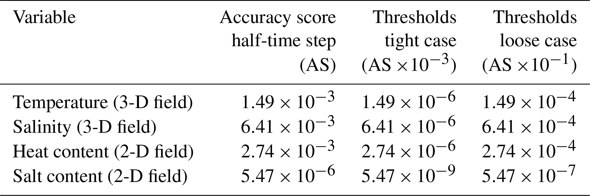
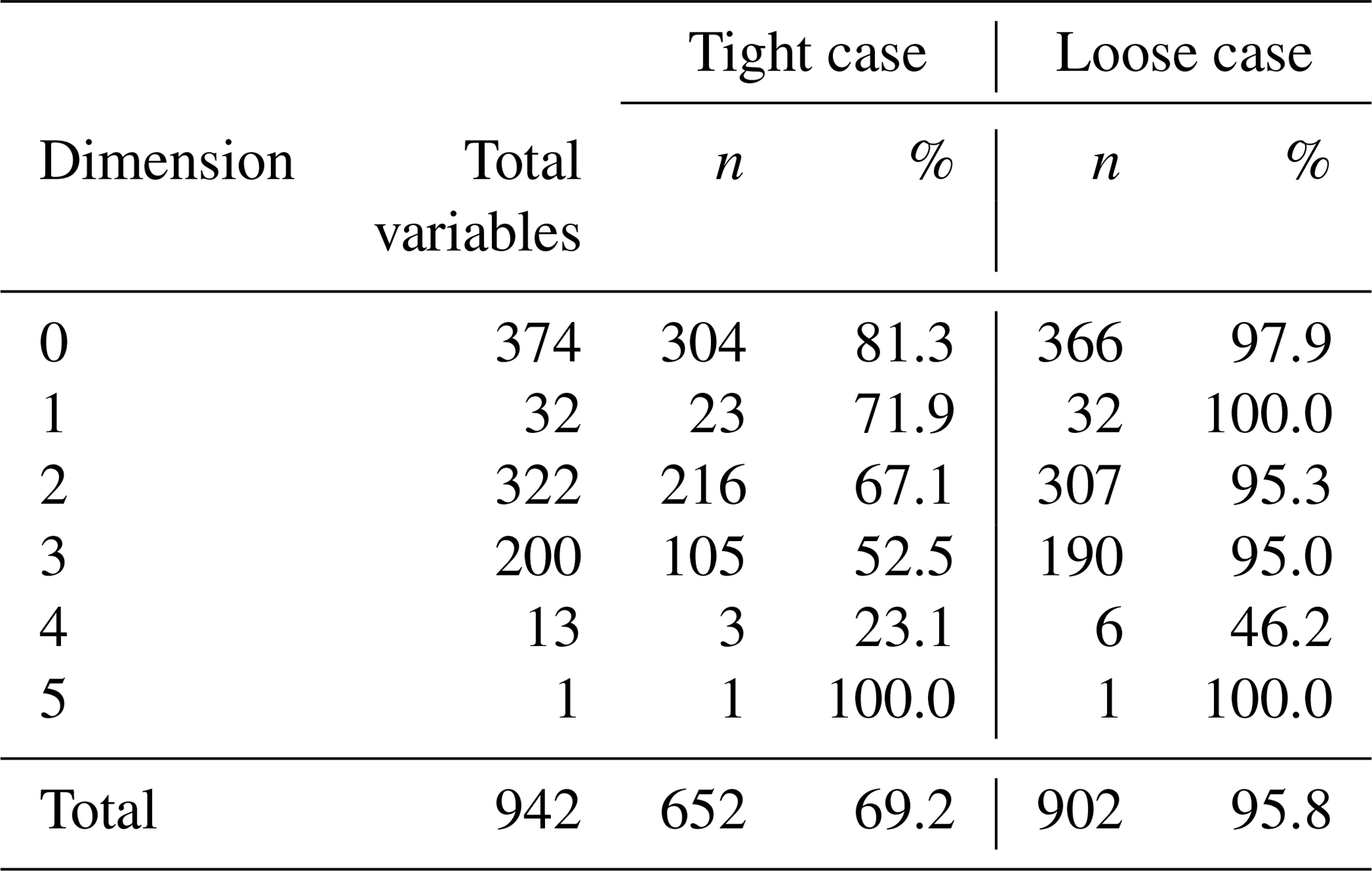
In order to define some meaningful thresholds, we performed a simulation using a halved time step to compute the accuracy score against the reference simulation; this value was used as a first guess to define our thresholds (see Table 1). To show how defining different thresholds leads to different results and to emphasize how with this method it is possible to keep arbitrarily small output differences, two different thresholds were defined (see Table 1). The first of the two thresholds is defined to be 1000 times smaller than the differences obtained using a halved time step. The second is defined to be only 10 times smaller. We will refer to these cases as the tight case and the loose case, respectively.
Table 1Accuracy score of the simulation performed using a time step shorter than the reference and the different thresholds used for the different variables in the tight and loose cases. The thresholds for the tight case are defined by multiplying the accuracy score of the half-time-step simulations by 10−3, and the thresholds for the loose case are defined by multiplying the accuracy score of the half-time step by 10−1.
3.1.3 Executing the tests
To execute the tests, we implemented the rules described in the Methods section by developing a Python workflow manager capable of handling the dynamic workflow by creating the simulation scripts, launching them on a remote platform, and then checking the status and adequacy of the results.
To perform tests, the Marenostrum 4 supercomputer has been used (see Table 2), with each individual simulation taking about 8 min 30 s on a single node.
During the implementation of the emulator, the declarations of more than 3500 real variables were replaced with emulator variables. These variables can be scalars or arrays of up to five dimensions. They can be global variables or just temporary variables used only in a single line of code inside a subroutine. In a large code like NEMO there are usually parts of the code that are either used or not depending on the specific parameters employed. For this reason, even when more than 3500 variables were identified, using our specific configuration only 942 are used. The variables that are used are identified during the runtime. Given that considering the unused variables for the analysis would be useless and dangerous (as incorrect conclusions could be drawn about what precision is needed) those are simply omitted from the analysis. The initial set used to start the analysis will therefore be the set containing the 942 variables that are actually used during our specific case.
3.1.4 Discussion
Starting with the evaluation of the initial set containing all the variables, the results show that a global reduction of the precision changes the results beyond what is acceptable. After running the full analysis for both cases we can see that the results differ. On the one hand, the tight case shows that 652 variables (69.2 %) could use single precision and, on the other hand, in the loose case the obtained solution contained 902 variables (95.8 %), thereby keeping only 40 variables in higher precision. As expected, defining looser thresholds allows for the use of lower precision in a larger portion of the variables. Table 3 presents the results split by array dimension. Also, the tighter case required more tests, with 1442 simulations required to arrive at the solution (consuming 204.3 node hours), while the loose case required only 321 (consuming 45.5 node hours).
The method ensures that the differences between the reduced-precision simulations performed with the final variable sets and the reference are below the determined thresholds. Although the accuracy test used for this example was not designed to ensure the conservation of global quantities, Fig. 1 shows that the global heat and salt content of the simulations performed using the loose configuration resembles those of the reference simulation performed fully in double precision, which was not the case for a simulation fully performed using single precision.
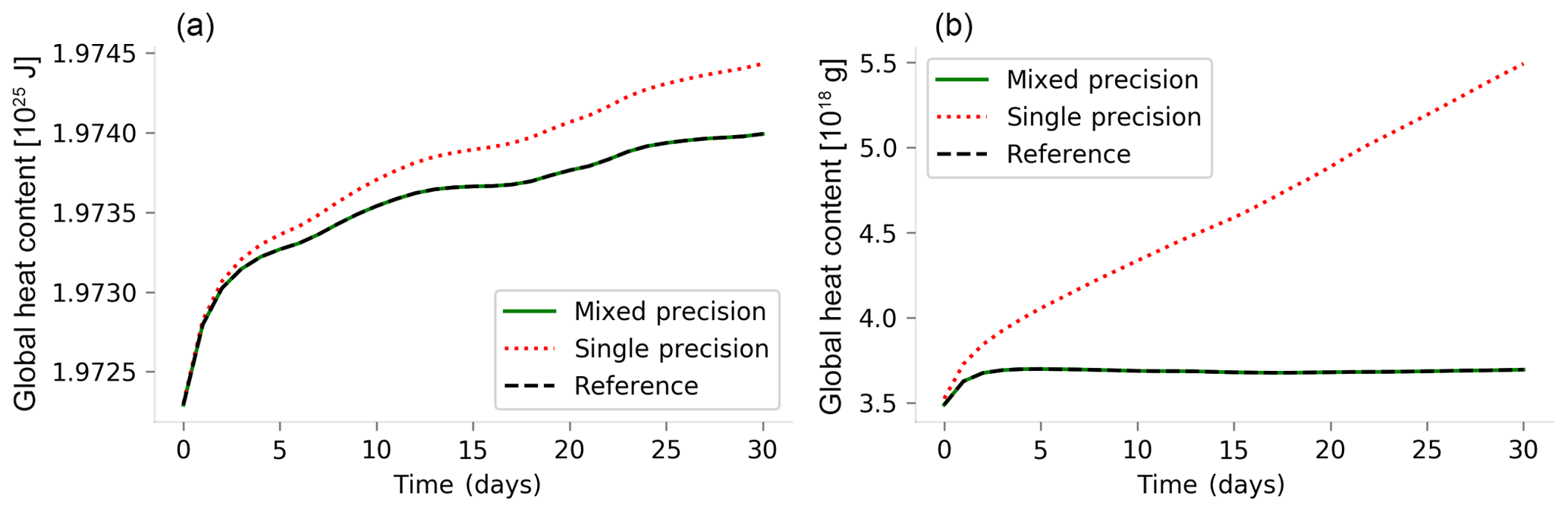
Figure 1Daily averages of the global heat content (a) and global salt content (b) for 1-month simulations using NEMO 4. The plot of the global salt content (b) has an offset of 4.731×10²² g. The reference simulation was performed using double precision, the single-precision simulation was performed using single-precision arithmetic for all the variables and the mixed-precision simulation was performed keeping 40 of the 942 model real variables in double precision and using single precision for the remaining 902 variables.
The Fig. 2 shows the expected impact on memory usage when using the set obtained with the loose accuracy test. Since the results produced by both cases are so close to the reference simulation, Fig. 2 only demonstrates the loose case because we anticipate that a mixed-precision implementation that is accepted by the scientific community would be more similar to the loose case.
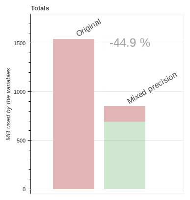
Figure 2Estimation of the memory usage impact in an ORCA2 configuration using the set obtained with the loose accuracy test. The estimation has been performed using the dimensions of the variables and the size of the domain. In red (darker) we have the memory that is occupied by variables in double precision (100 % in the original case), and in light green the proportion of the memory occupied by variables in single precision; the difference between the original case and the loose case implies a potential 44.9 % decrease in memory usage.
Table 3The table presents the total number of variables that were included in the analysis split by the dimension of the arrays (0 for scalars). Also shown are the number of variables that can safely use single precision for the two cases discussed in Sect. 3.1 (tight and loose) and the percentage of the total variables that this represents. Using tight constraints, 69.2 % of the variables can use single precision, although only 52.5 % of the 3-D variables are responsible for the most memory usage. Using loose conditions, 95.8 % of the variables can use single precision, including 95 % of the 3-D variables.
3.2 ROMS
The Regional Ocean Modeling System (ROMS) is a free-surface, hydrostatic, primitive-equation ocean model that uses stretched, terrain-following coordinates on the vertical and orthogonal curvilinear coordinates on the horizontal. It contains a variety of features, including high-order advection schemes, accurate pressure gradient algorithms, several subgrid-scale parameterizations, atmospheric, oceanic, and benthic boundary layers, biological modules, radiation boundary conditions, and data assimilation (http://www.myroms.org, last access: 18 October 2018).
The experiments performed with ROMS were done by applying the primal form of the incremental strong constraint 4D-Var (4DVAR) (Moore et al., 2011). The configuration used is the US west coast at 1∕3∘ horizontal, referred to as WC13, a standard model test case. It has ∼30 km horizontal resolution and 30 levels on the vertical (http://www.myroms.org, last access: 18 October 2018). This configuration was selected because 4DVAR ROMS has a large community of users, there is an easy-to-follow tutorial to set up the configuration and it involves linear models that make this an interesting choice to expand the results obtained in Sect. 3.1.
To perform this analysis, we set up the tutorial available online that performs an I4DVAR data assimilation cycle that spans the period 3–6 January 2004. The observations assimilated into the model are satellite sea surface temperature, satellite sea surface height in the form of a gridded product from Aviso, and hydrographic observations of temperature and salinity collected from Argo floats and during the GLOBEC/LTOP and CalCOFI cruises off the coast of Oregon and southern California, respectively.
With the I4DVAR version of ROMS, most of the computational time is spent inside the data assimilation “inner loops” within the adjoint and tangent linear sub-models (AD and TL, respectively). To give some numbers, in a simulation with the WC13 configuration, 35 % of the time is spent in the TL model and 50 % in the AD model, while the time spent in the nonlinear model is below 14 %. It was felt that since the TL and AD models are used to compute an approximation gradient of the I4DVAR cost function, further approximations in the gradient resulting from lower precision will probably be not so detrimental, leading to our starting hypothesis that the AD and TL models are better targets than the nonlinear model. However, for this hypothesis to be true the AD needs to keep being the transpose of the TL to within a chosen precision; otherwise, it might prevent the convergence of the algorithm. For this reason, we are trying to minimize the precision used in these regions of the code. In this case, the target reduced precision is not limited to single precision (23-bit significand), but the half-precision is also explored (10-bit significand).
It is important to remark that in our experiments the number of bits used to represent the exponent of the variables is 11 (the same number as used in double precision), no matter what number of bits is used for the significand. In practice, it means that to ensure that it is possible to reduce the precision to half-precision we would need to ensure that the values do not exceed the range that can be represented with a smaller exponent. However, the results are still interesting because we can learn the potential use of a reduced number of bits for the significand.
3.2.1 Emulator implementation
One aspect that made this exercise different from that of NEMO in terms of implementing the emulator was that the interest was focused on specific regions of the code, i.e., the parts related to the tangent linear model and the adjoint model.
3.2.2 Designing the tests
When running a data assimilation experiment, the objective is to obtain a coherent state of the ocean that minimizes the difference between the model and the observations. Through different forward–backward iterations using the TL and AD models, the model should converge to a state in which the cost function (function that describes the difference between the model state and the observations) is minimum. We can consider a simulation to be accurate enough if the model converges to the same result as the double-precision reference. Through the different iterations, the solution should converge to a minimum. To set a threshold for the accuracy of the simulations, we can look at the difference between the last two inner-loop iterations. In the reference simulation the value of this difference computed as a cost function defined in the model is . Defining a threshold 10 times smaller () ensures that the impact of reducing the precision will be smaller than changing the number of inner iterations performed.
3.2.3 Executing the tests
For ROMS, we use the same workflow manager developed for NEMO, simply using different templates for launching simulations and evaluating the results.
3.2.4 Discussion
As in the case with NEMO, we first performed the reference executions for all the different initial conditions using 64-bit precision.
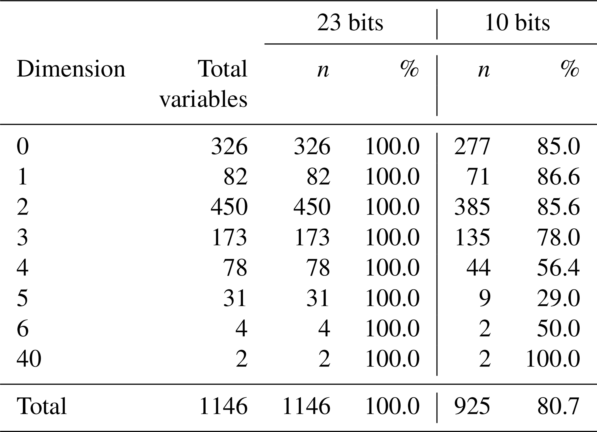
The parts selected for the analysis contain 1556 real-variable declarations, 1144 of which are actually used in our case. Starting with this initial set and trying to use a 23-bit significand, the results showed that in fact all the variables can use reduced precision at once while still obtaining accurate results.
This suggests that this model and in particular this specific configuration are suitable for a more drastic reduction of the numerical precision. To test that, we proceeded with a new analysis using a 10-bit significand. The first simulation of the analysis crashed, not providing any output and showing that it is not possible to reduce the precision to 10 bits overall. Using the analysis to find where this precision can be used, the results show that 80.7 % of the variables can use 10 bits instead of 52. Looking to the effects produced by the variables that were not able to use 10-bit precision we could see that only a single variable was preventing the model from completing the simulations, even though many others were introducing too many numerical errors. In Table 4 the results are presented split by dimension.
Table 4The table presents the total number of variables that were included in the ROMS analysis split by the dimension of the arrays (0 for scalars). Also shown are the number of variables that can safely use reduced precision for the two cases discussed in Sect. 3.2 (single precision and half-precision) and the percentage of the total variables that they represent. The single-precision case was trivial since all the variables considered can use single precision while keeping the accuracy. For the half-precision case, 80.7 % of the variables could use half-precision, although the proportion of variables that can use reduced precision becomes lower as the dimension increases.
3.3 Common discussion
From the two exercises shown in Sect. 3 we can draw several conclusions. The most important is that the method can provide a set of variables that can use reduced numerical precision while preserving the accuracy of the results, as was observed in the four cases explored (two different accuracy tests for NEMO and two target precisions for ROMS). The results in the four cases showed that the potential to reduce the numerical precision is considerable even in the most constrained cases (i.e., NEMO tight). In the NEMO case, the analysis covers the full model, while the ROMS case was focused only on a part of the model, demonstrating the versatility of the method. It has also been shown that it is possible to achieve results that are arbitrarily close to the reference, while requiring more exact results will have the cost of leaving more parts of the code in higher precision.
Previous works suggested that the generalized use of double precision for Earth science modeling is a case of overengineering and that for this reason adapting the computational models to use the smallest numerical precision that is essential would compensate in terms of improvement in performance. However, an improper reduction can lead to accuracy losses that may make the results unreliable. In this paper we presented a method that was designed to solve this problem by finding which variables can use a lower level of precision without degrading the accuracy of the results.
The method was designed to be applied to computational ocean models coded in Fortran. It relies on the Reduced Precision Emulator tool, which was created to help us understand the effect of reduced precision within numerical simulations. It allows us to simulate the results that would be produced in the case of performing arithmetic operations in reduced precision using a custom number of significant bits for each floating-point variable. The proposed analysis algorithm finds which variables need to be kept in double precision and which ones can use reduced precision without impacting the accuracy of the results.
The method has been tested with two widely used state-of-the-art ocean models, NEMO and ROMS. The experiences with the two models pursued different objectives. With NEMO, the analysis covered all the routines and variables used within the ocean-only simulation; the target precision was 32 bits, and we explored how the selection of specific accuracy tests changes which variables can safely use reduced precision. However, with ROMS, the analysis covered only the variables belonging to the adjoint and tangent linear models using a single accuracy test and examining how the method can be used to discover the viability of using numerical precisions below 32 bits.
The results presented in this work allow us to draw some conclusions. It is shown that both models can use reduced precision for large portions of the code, proving the feasibility of mixed-precision approaches, and the method described is able to find these. The method can also provide a configuration that can be arbitrarily close to the double-precision reference, whereby the amount of variables that can use reduced precision will depend on how strict the imposed conditions are.
Users might want to follow the method presented here to build a version of the model that can benefit from a reduction of precision and can be used by the whole community without concerns.
Releases of the Reduced Precision Emulator library are available at https://github.com/aopp-pred/rpe (Dawson and Dueben, 2016, last access: January 2019). The tool developed to automatically implement RPE can be found at https://earth.bsc.es/gitlab/otinto/AutoRPE (Tintó Prims, 2019). The workflow manager used to manage the analysis simulations can be found at https://earth.bsc.es/gitlab/otinto/AutoRPE (Tintó Prims, 2019). The source code of the NEMO model and the input data used for the experiments referred to in this work can be found at https://www.nemo-ocean.eu/ (last access: January 2019). The source code of the ROMS model can be found at http://www.myroms.org/ (The ROMS/TOMS Group, 2019) and can be freely accessed under registration. The details and input data used for the experiments involving ROMS can be found at https://www.myroms.org/wiki/I4DVAR_Tutorial (last access: January 2019).

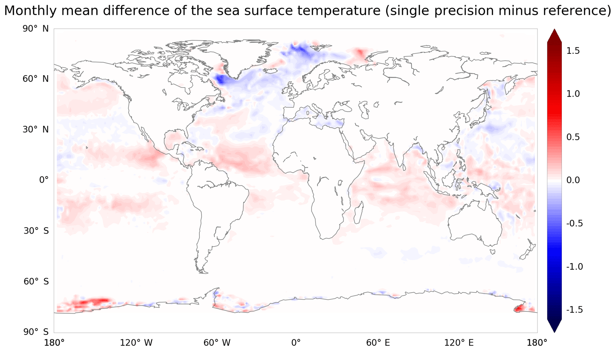
Figure B1Difference in sea surface temperature monthly mean (∘C) for the first month of simulation between a NEMO 4.0 simulation performed emulating single-precision arithmetic and a NEMO 4.0 simulation performed using double-precision arithmetic. The monthly mean of the sea surface temperature for the first month of simulation shows localized biases exceeding 1.5 ∘C.
OTP led the design of the method, the experiments and the writing of the paper. MCA supervised all the processes and had a main role in the writing of the paper. AMM participated in the design of the experiments involving ROMS and the writing of the paper. MC was involved in the discussion and design of the method and the experiments and participated in the writing of the paper. KS, AC and FJD participated in the discussions and the revision of the paper.
The authors declare that they have no conflict of interest.
The research leading to these results has received funding from the EU ESiWACE H2020 Framework Programme under grant agreement no. 823988, from the Severo Ochoa (SEV-2011-00067) program of the Spanish Government and from the Ministerio de Economia y Competitividad under contract TIN2017-84553-C2-1-R.
This paper was edited by Steven Phipps and reviewed by Peter Düben and Matthew Chantry.
Aumont, O., Ethé, C., Tagliabue, A., Bopp, L., and Gehlen, M.: PISCES-v2: an ocean biogeochemical model for carbon and ecosystem studies, Geosci. Model Dev., 8, 2465–2513, https://doi.org/10.5194/gmd-8-2465-2015, 2015. a
Baboulin, M., Buttari, A., Dongarra, J., Kurzak, J., Langou, J., Langou, J., Luszczek, P., and Tomov, S.: Accelerating scientific computations with mixed precision algorithms, Comput. Phys. Commun., 180, 2526–2533, https://doi.org/10.1016/j.cpc.2008.11.005, 2009. a, b, c
Bauer, P., Thorpe, A., and Brunet, G.: The quiet revolution of numerical weather prediction, Nature, 525, 47–55, https://doi.org/10.1038/nature14956, 2015. a, b
Bellard, C., Bertelsmeier, C., Leadley, P., Thuiller, W., and Courchamp, F.: Impacts of climate change on the future of biodiversity, Ecol. Lett., 15, 365–377, https://doi.org/10.1111/j.1461-0248.2011.01736.x, 2012. a
Dawson, A. and Dueben, P.: aopp-pred/rpe: v5.0.0 (Version v5.0.0), Zenodo, https://doi.org/10.5281/zenodo.154483, 2016. a
Dawson, A. and Düben, P. D.: rpe v5: an emulator for reduced floating-point precision in large numerical simulations, Geosci. Model Dev., 10, 2221–2230, https://doi.org/10.5194/gmd-10-2221-2017, 2017. a, b, c
Dennis, J. M. and Loft, R. D.: Refactoring Scientific Applications for Massive Parallelism, in: Numerical Techniques for Global Atmospheric Models, 80, 539–556, https://doi.org/10.1007/978-3-642-11640-7_16, 2011. a
Düben, P. D., McNamara, H., and Palmer, T. N.: The use of imprecise processing to improve accuracy in weather & climate prediction, J. Comput. Phys., 271, 2–18, https://doi.org/10.1016/j.jcp.2013.10.042, 2014. a
Düben, P. D., Subramanian, A., Dawson, A., and Palmer, T. N.: A study of reduced numerical precision to make superparameterization more competitive using a hardware emulator in the OpenIFS model, J. Adv. Model. Earth Sy., 9, 566–584, https://doi.org/10.1002/2016MS000862, 2017. a
Düben, P. D., Subramanian, A., Dawson, A., and Palmer, T. N.: A study of reduced numerical precision to make superparameterization more competitive using a hardware emulator in the OpenIFS model, J. Adv. Model. Earth Sy., 9, 566–584, https://doi.org/10.1002/2016MS000862, 2017. a
Graillat, S., Fabienne, J., Picot, R., and Lathuili, B.: PROMISE: floating-point precision tuning with stochastic arithmetic, 17th international symposium on Scientific Computing, Computer Arithmetic and Verified Numerics (SCAN 2016), UPPSALA, Sweden, 98–99, September 2016. a
Haidar, A., Tomov, S., Dongarra, J., and Higham, N. J.: Harnessing GPU Tensor Cores for Fast FP16 Arithmetic to Speed up Mixed-Precision Iterative Refinement Solvers, in: Proceedings of the International Conference for High Performance Computing, Networking, Storage, and Analysis, SC'18 (Dallas, TX), IEEE Press, Piscataway, NJ, USA, 47:1–47:11, available at: http://dl.acm.org/citation.cfm?id=3291656.3291719 (last access: July 2019), 2018. a
Hegerl, G. and Zwiers, F.: Use of models in detection and attribution of climate change, Wires Clim. Change, 2, 570–591, https://doi.org/10.1002/wcc.121, 2011. a
Kniveton, D. R., Smith, C. D., and Black, R.: Emerging migration flows in a changing climate in dryland Africa, Nat. Clim. Change, 2, 444–447, https://doi.org/10.1038/nclimate1447, 2012. a
Lam, M. O., De Supinksi, B. R., Legendre, M. P., and Hollingsworth, J. K.: Automatically adapting programs for mixed-precision floating-point computation, Proceedings – 2012 SC Companion: High Performance Computing, Networking Storage and Analysis, SCC 2012, 1423–1424, https://doi.org/10.1109/SC.Companion.2012.231, 2012. a
Madec, G.: NEMO ocean engine, Note du Pole de modelisatio 1288–1619, https://www.nemo-ocean.eu/wp-content/uploads/Doc_OPA8.1.pdf (last access: July 2019), 2008. a
Moore, A., Arango, H., Broquet, G., S. Powell, B., Weaver, A., and Zavala-Garay, J.: The Regional Ocean Modeling System (ROMS) 4-dimensional variational data assimilation systems Part I – System overview and formulation, Prog. Oceanogr., 91, 34–49, https://doi.org/10.1016/j.pocean.2011.05.004, 2011. a
Oreskes, N., Stainforth, D. A., and Smith, L. A.: Adaptation to Global Warming: Do Climate Models Tell Us What We Need to Know?, Philos. Sci., 77, 1012–1028, https://doi.org/10.1086/657428, 2010. a
Palmer, T., Shutts, G., Hagedorn, R., Doblas-Reyes, F., Jung, T., and Leutbecher, M.: Representing model uncertainty in wheather and climate prediction, Annu. Rev. Earth Pl. Sc., 33, 163–193, https://doi.org/10.1146/annurev.earth.33.092203.122552, 2005. a
Randall, D., Wood, R., Bony, S., Colman, R., Fichefet, T., Fyfe, J., Kattsov, V., Pitman, A., Shukla, J., Srinivasan, J., Stouffer, R., Sumi, A., and Taylor, K.: Climate Models and Their Evaluation, in: IPCC, 2007: Climate Change 2007: the physical science basis. contribution of Working Group I to the Fourth Assessment Report of the Intergovernmental Panel on Climate Change, 323, 589–662, https://doi.org/10.1016/j.cub.2007.06.045, 2007. a
Rousset, C., Vancoppenolle, M., Madec, G., Fichefet, T., Flavoni, S., Barthélemy, A., Benshila, R., Chanut, J., Levy, C., Masson, S., and Vivier, F.: The Louvain-La-Neuve sea ice model LIM3.6: global and regional capabilities, Geosci. Model Dev., 8, 2991–3005, https://doi.org/10.5194/gmd-8-2991-2015, 2015. a
The ROMS/TOMS Group: ROMS, available at: http://www.myroms.org/, last access: July 2019. a
Thornes, T.: Can reducing precision improve accuracy in weather and climate models?, Weather, 71, 147–150, https://doi.org/10.1002/wea.2732, 2016. a
Tintó Prims, O.: AutoRPE, available at: https://earth.bsc.es/gitlab/otinto/AutoRPE, last access: July 2019. a, b
Tintó Prims, O., Castrillo, M., Acosta, M., Mula-Valls, O., Sanchez Lorente, A., Serradell, K., Cortés, A., and Doblas-Reyes, F.: Finding, analysing and solving MPI communication bottlenecks in Earth System models, J. Comput. Sci., https://doi.org/10.1016/j.jocs.2018.04.015, in press, 2018. a
Váňa, F., Düben, P., Lang, S., Palmer, T., Leutbecher, M., Salmond, D., and Carver, G.: Single Precision in Weather Forecasting Models: An Evaluation with the IFS, Mon. Weather Rev., 145, 495–502, https://doi.org/10.1175/MWR-D-16-0228.1, 2017. a
Whiteman, G. and Hope, C. W. P.: Vast costs of Arctic change, Nature, 499, 401–403, https://doi.org/10.1038/499401a, 2013. a