the Creative Commons Attribution 4.0 License.
the Creative Commons Attribution 4.0 License.
 | 25 Jul 2019
How can the First ISLSCP Field Experiment contribute to present-day efforts to evaluate water stress in JULESv5.0?
Karina E. Williams
Anna B. Harper
Chris Huntingford
Lina M. Mercado
Camilla T. Mathison
Pete D. Falloon
Peter M. Cox
Joon Kim
The First International Satellite Land Surface Climatology Project (ISLSCP) Field Experiment (FIFE), Kansas, US, 1987–1989, made important contributions to the understanding of energy and CO2 exchanges between the land surface and the atmosphere, which heavily influenced the development of numerical land-surface modelling. Now, 30 years on, we demonstrate how the wealth of data collected during FIFE and its subsequent in-depth analysis in the literature continue to be a valuable resource for the current generation of land-surface models. To illustrate, we use the FIFE dataset to evaluate the representation of water stress on tallgrass prairie vegetation in the Joint UK Land Environment Simulator (JULES) and highlight areas for future development. We show that, while JULES is able to simulate a decrease in net carbon assimilation and evapotranspiration during a dry spell, the shape of the diurnal cycle is not well captured. Evaluating the model parameters and results against this dataset provides a case study on the assumptions in calibrating “unstressed” vegetation parameters and thresholds for water stress. In particular, the responses to low water availability and high temperatures are calibrated separately. We also illustrate the effect of inherent uncertainties in key observables, such as leaf area index, soil moisture and soil properties. Given these valuable lessons, simulations for this site will be a key addition to a compilation of simulations covering a wide range of vegetation types and climate regimes, which will be used to improve the way that water stress is represented within JULES.
- Article
(10117 KB) -
Supplement
(543 KB) - BibTeX
- EndNote


The works published in this journal are distributed under
the Creative Commons Attribution 4.0 License. This license does not affect
the Crown copyright work, which is re-usable under the Open Government
Licence (OGL). The Creative Commons Attribution 4.0 License and the OGL are
interoperable and do not conflict with, reduce or limit each
other.
© Crown copyright 2019
Models of the land surface and biosphere, a key component in climate predictions and projections, depend on high-quality observational datasets to tune the behaviour of the modelled processes. A significant contribution in this field was produced by the First International Satellite Land Surface Climatology Project (ISLSCP) Field Experiment (FIFE), an interdisciplinary collaboration of researchers from remote sensing, atmospheric physics, meteorology and biology. It was based at and around the Konza Prairie Long-Term Ecological Research (LTER) site, Kansas, during multiple campaigns, 1987–1989. Its principal objectives were twofold: to improve the understanding of the role of biological processes in controlling atmosphere–surface exchange of heat, water vapour and CO2, and to investigate whether satellite observations can constrain land-surface parameters relevant to the climate system (Sellers et al., 1988; Sellers and Hall, 1992).
As part of this experiment, canopy processes were related to leaf-level stomatal conductance, photosynthesis and respiration, including detailed modelling of responses to water availability and atmospheric forcing (Verma et al., 1989, 1992; Kim and Verma, 1990b, a, 1991a, b; Kim et al., 1992; Stewart and Verma, 1992; Norman et al., 1992; Niyogi and Raman, 1997; Cox et al., 1998; Colello et al., 1998). This work has subsequently played an important role in influencing the representation of vegetation in a generation of land-surface models. The parameterisation of water stress in the Joint UK Land Environment Simulator (JULES) (Best et al., 2011; Clark et al., 2011), for example, originates in a canopy conductance and photosynthesis model presented in Cox et al. (1998), which was developed using FIFE observations. After tuning, the Cox et al. (1998) model gave a very good fit to the data: it explained 91.7 % of the variance in net canopy photosynthesis and 89.4 % of the variance in canopy conductance, as derived from FIFE flux tower observations. As part of this model, Cox et al. (1998) calculated a piecewise-linear stress factor β. This factor is zero below the wilting soil moisture and one above a critical soil moisture (Fig. 1, solid line), based on the top 1.4m of soil. Crucially, Cox et al. (1998) found that the drop in carbon assimilation in the C4 vegetation as soil water content decreased at FIFE could only be reproduced if the stress factor β was applied directly to the net leaf assimilation rate. In their model, soil water stress affected stomatal conductance via the net leaf assimilation rate.
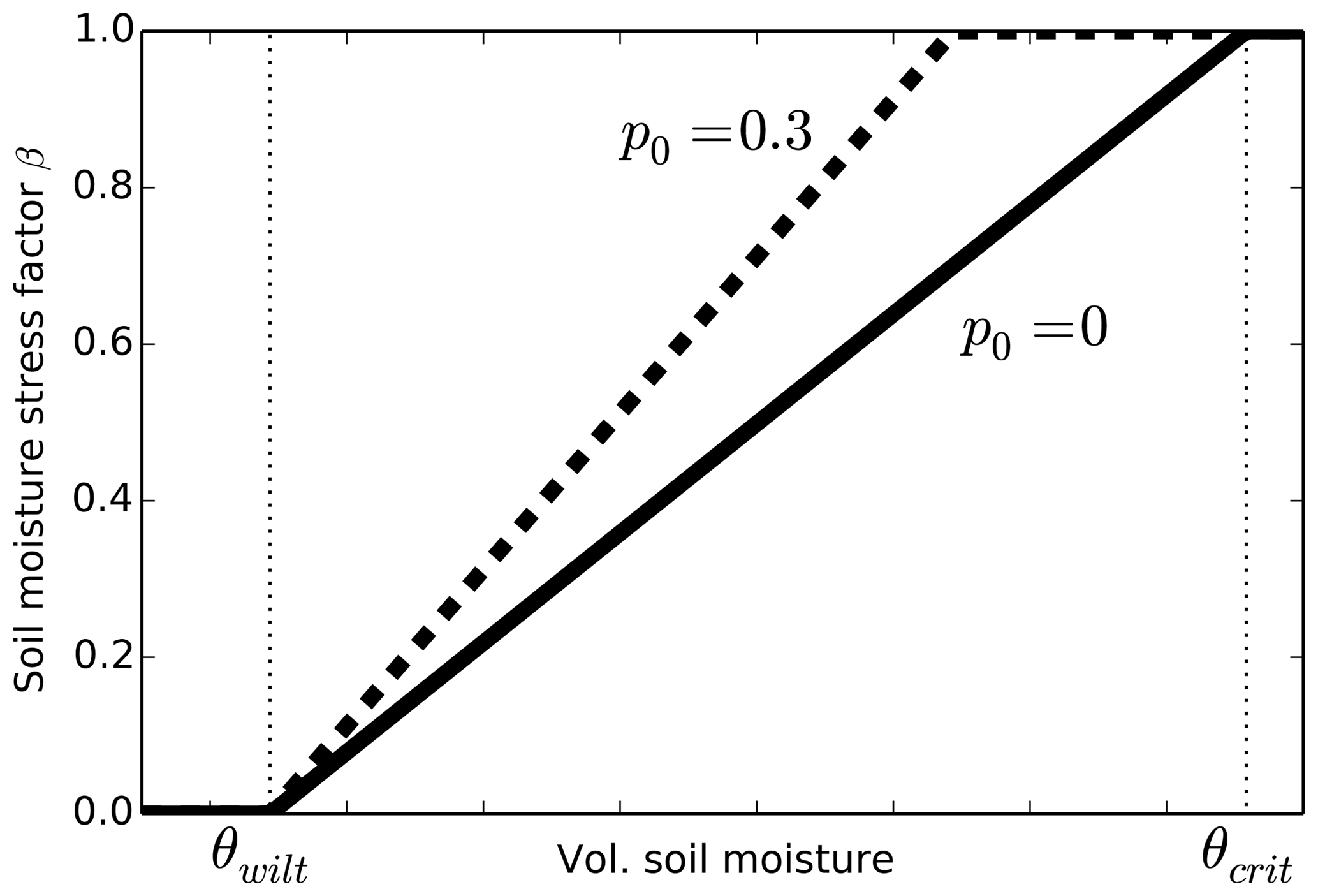
Figure 1JULES soil moisture stress factor β with p0=0 (solid line) and p0=0.3 (dashed line). The soil moisture threshold at which the plant becomes completely unstressed (β=1) is .
The Cox et al. (1998) stress parameterisation was adopted in early versions of JULES. It was the only implementation of soil moisture stress in JULES until version 4.6 and, to our knowledge, has been used in all published studies to date. The JULES wilting and critical soil moisture values are input by users for each soil layer in each grid box and are defined as corresponding to absolute matric water potentials of 1.5 and 0.033 MPa, respectively (Best et al., 2011). A separate stress factor is calculated for each soil layer, and these are combined into an overall soil moisture stress factor by weighting by the root mass distribution. Other options have been more recently implemented into JULES. These include a “bucket” approach, in which the stress factor β is calculated from the average soil moisture to a specified depth, and the introduction of a new variable p0 which reduces the soil moisture at which a vegetation type first starts to experience water stress (Fig. 1, dashed line).
There is currently a community-wide effort to improve the response of JULES to drought conditions. This effort requires a large amount of data to evaluate against, covering a wide variety of climates and vegetation types, in order to give confidence in the underlying representation of this process in the model. This is vital if the model is to be used to simulate global responses to changes in water availability in the future.
Observations taken during the FIFE campaign are still available today, through the Oak Ridge National Laboratory Distributed Active Archive Center (ORNL DAAC). Given that FIFE observations were fundamental to the development of the original water stress parameterisation in JULES, we revisit this dataset to determine whether it would make a useful contribution to present-day efforts to improve this process. We aim to demonstrate that there are sufficient data available, and of a sufficient quality, to show that the current version of JULES is unable to capture key features of the impact of water availability on the temperate grassland vegetation at the FIFE site. This can provide a benchmark for this vegetation type, against which future model developments can be assessed. We thus hope to encourage the inclusion of this dataset in comprehensive, multi-site studies that aim to improve the representation of this process on a global scale.
We first create a simulation that closely reproduces the Cox et al. (1998) study, in order to investigate how this original study was able to provide such a close fit to the observed carbon and water fluxes at FIFE. Our second configuration uses more recent model developments, with parameter values based on the generic C4 grass tile from the global analysis of Harper et al. (2016). These settings are typical for how this vegetation type is usually represented in current-day runs of JULES. We then use FIFE observations to tune some of these generic C4 grass parameters to more accurately represent tallgrass prairie. The aim here is to allow us to distinguish between model limitations due to approximating this specific vegetation type by generic C4 grass parameters and model limitations due to missing or inadequately represented processes within the model. The model setup for each of these simulations is described in Sect. 2. In Sect. 3, we compare the results from the model simulations to net canopy carbon assimilation, derived from CO2 flux measurements, and latent heat energy flux measurements at the FIFE site. We conclude with a summary of what lessons can be learnt for improving water stress in JULES from FIFE and how this dataset can be useful to the JULES community into the future. Throughout, we refer to the appendices, which give more information about the use of the observations and the alternative datasets considered, in order to assist future modelling work at this site, both with JULES and other land-surface models. A important component of this study is the provision of a complete JULES setup that can be downloaded and used to run FIFE data through the JULES model, to allow easy inclusion of this site into a comprehensive evaluation framework for JULES.
We will focus on three different configurations of JULES:
-
Simulation 1 (
repro-cox-1998) is a simplified JULES run, which reproduces the original Cox et al. (1998) study as closely as possible. This requires the simple “big leaf” canopy scheme, prescribes the leaf area index (LAI) and soil moisture from observations and calculates the soil moisture stress from the average soil moisture in the top 1.4 m of soil. -
Simulation 2 (
global-C4-grass) uses parameter settings from Harper et al. (2016), which has a generic representation of C4 grass. It uses many of the “state-of-the-art” features of JULES, such as the layered canopy scheme with sunflecks, and calculates soil moisture stress using a weighted sum of the stress factors in each soil layer. LAI and soil moisture are prescribed. -
Simulation 3 (
tune-leaf) is as above, but we investigate whether the generic C4 grass leaf parameters can be tuned to site measurements, to give a more accurate representation of the prairie vegetation.
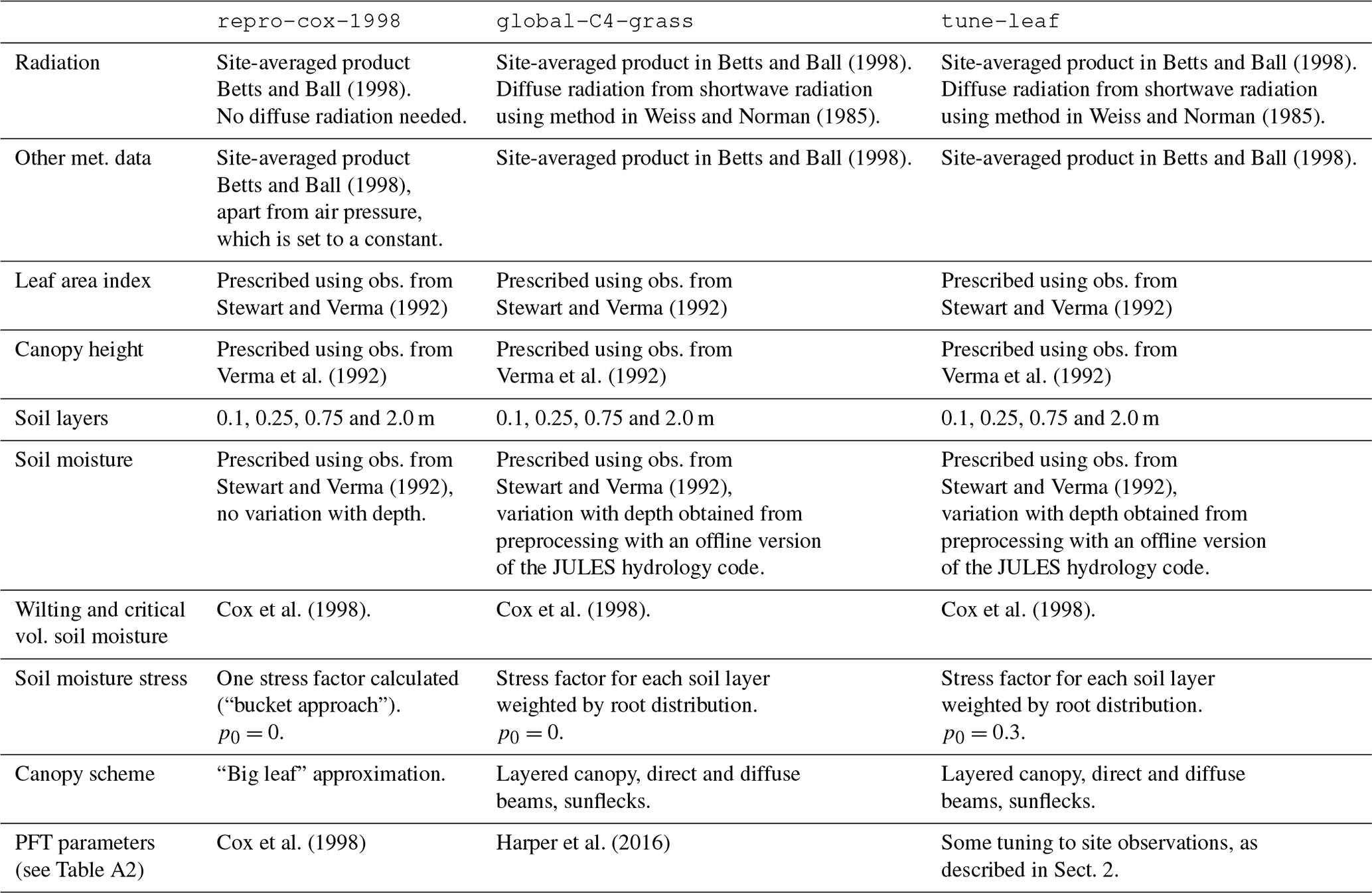
These configurations are described below and summarised in Table 1. All the FIFE datasets used in this study are given in Table A1.
Betts and Ball (1998)Betts and Ball (1998)Betts and Ball (1998)Weiss and Norman (1985)Weiss and Norman (1985)Betts and Ball (1998)Betts and Ball (1998)Betts and Ball (1998)Stewart and Verma (1992)Stewart and Verma (1992)Stewart and Verma (1992)Verma et al. (1992)Verma et al. (1992)Verma et al. (1992)Stewart and Verma (1992)Stewart and Verma (1992)Stewart and Verma (1992)Cox et al. (1998)Cox et al. (1998)Cox et al. (1998)Cox et al. (1998)Harper et al. (2016)Table 1Model settings for the runs at FIFE site 4439 for 1987. Further descriptions of the model setup can be found in Sect. 2 and the choice of FIFE observations in Sect. A.
2.1 Simulation 1: repro-cox-1998
Our first simulation, repro-cox-1998, closely reproduces the optimal
configuration presented in the Cox et al. (1998) study.
Cox et al. (1998) modelled the fluxes for FIFE site 4439 (situated at
39∘03′ N, 96∘32′ W; 445 m above mean sea level). This
tallgrass prairie site is roughly central within the 15 km × 15 km FIFE
study area. It had been lightly grazed by domestic livestock but was
ungrazed in 1986 and 1987 and was burned on 16 April 1987
(Kim and Verma, 1990a, 1991b). At the flowering stage in
1987, more than 80 % of the vegetation was composed of C4 grasses
(Kim and Verma, 1990a).
For their analysis, Cox et al. (1998) selected daylight hours that were both after 10:00 LT, to exclude dew evaporation, and from days with no rainfall during that day or the preceding day. This minimised the effect of evaporation of rainfall from the canopy and soil surface and let them focus on modelling transpiration and net canopy assimilation. We will also restrict our analysis to these same time periods. The model was spun up by repeating the entire run 10 times, and the output from the 11th run was analysed.
For driving data, we use a site-averaged product of the FIFE portable Automatic Meteorological Station (AMS) data at 30 min resolution (Betts and Ball, 1998). We prescribe both LAI and soil moisture from observations (Stewart and Verma, 1992) rather than calculating these variables internally using the JULES phenology or soil hydrology schemes. We use a “bucket approach” to calculate the soil moisture stress factor from the average soil moisture in the top 1.4 m (this option has been available from JULES 4.6 onwards), again to mimic the Cox et al. (1998) analysis. The wilting soil moisture θwilt was set to 0.205 m3 m−3 and the critical soil moisture θcrit was set to 0.387 m3 m−3, taken directly from Cox et al. (1998). The resulting stress factor is plotted in Fig. 2 and clearly shows the dry period during late July and early August.
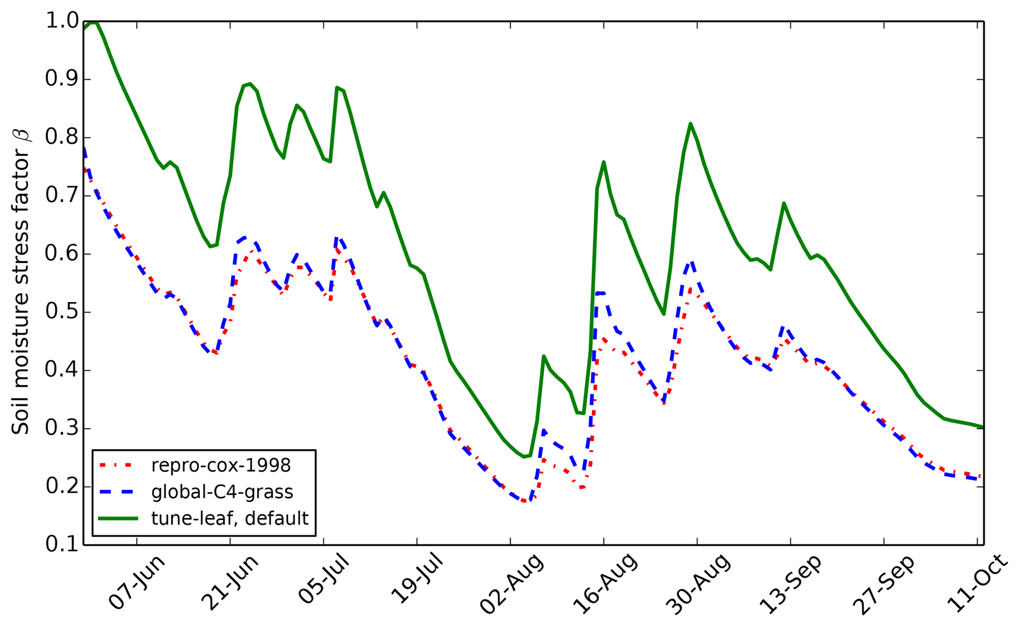
Figure 2Daily mean soil moisture stress factor β for each JULES simulation at FIFE site 4439 in 1987.
JULES and the Cox et al. (1998) optimal configuration both use the Collatz et al. (1992) C4 photosynthesis scheme. They also both use the same stomatal conductance parameterisation: Jacobs (1994), which is in turn a simplified version of the Leuning (1995) scheme. We select the “big leaf” option from the available canopy schemes in JULES, again to mimic Cox et al. (1998).
In this way, we are able to closely reproduce the Cox et al. (1998) calculation of daytime net canopy carbon assimilation and daytime canopy conductance with a modern version of JULES. Any remaining differences are minor. For example, in Cox et al. (1998), leaf temperature is calculated from the air temperature and observed sensible heat flux, whereas, in JULES, the full energy balance is modelled. There are also differences in the calculation of evaporation from soil and canopy, which are not the focus of this study. The calculation of aerodynamic resistance also differs. For example, in this run, canopy height is prescribed using the data from Verma et al. (1992) for this site in 1987 (see Sect. A5 for more information), whereas it was not modelled explicitly as part of the Cox et al. (1998) analysis.
Many of the key FIFE datasets used in this run have large uncertainties, despite being comprehensively measured by multiple teams. LAI measurements have an error of approximately 75 % due to the inherent variability of prairie vegetation. LAI measurements are also affected by leaf curling or folding as the leaves pass through the detector. There are therefore significant differences between datasets (for a more detailed description, see Sect. A2). For example, at the beginning of August, LAI measurements vary from 2.5 (Stewart and Verma, 1992) to 0.7 (the FIFE_VEG_BIOP_135 dataset). Soil moisture was also comprehensively measured across the FIFE area by multiple groups (see Sect. A3). While these observations are qualitatively consistent, one of the datasets shows a bias in the lower soil levels at site 4439 in 1987 compared to the other datasets. Within-site variability in soil moisture is also large. Soil properties were similarly well studied: there are four different datasets which can be used to calculate the wilting and critical soil moisture values, plus the values from two additional published studies (described in Sect. A4). However, measurements differ from each other by more than 0.15 m3 m−3 in some cases. There also appear to be differences between layers, with the top 10 cm having consistently lower wilting and critical thresholds than soil at a depth of about 30 cm, for example. It is therefore vital that we consider the implications of the spread in observed LAI, soil moisture and soil properties at this site when drawing our conclusions.
2.2 Simulation 2: global-C4-grass
In our second simulation, we use a recent JULES configuration, presented in
Harper et al. (2016). This study introduced a trait-based approach to
calculating leaf physiology in JULES and tuned plant parameters to
observations in the TRY database (Kattge et al., 2011). Global vegetation was
split into nine plant functional types (PFTs), including one to represent all C4
grasses. The developments introduced in Harper et al. (2016) resulted in
improved site-scale and global simulations of plant productivity and global
vegetation distributions (Harper et al., 2018). Our
global-C4-grass configuration is based on the representation of C4
grasses in Harper et al. (2016) and takes advantage of many of the
modern features of JULES. This includes a layered canopy scheme that treats
the direct and diffuse components of the incident radiation separately (as in
Sellers, 1985) and includes sunflecks (Dai et al., 2004; Mercado et al., 2007, 2009). It also calculates the overall soil
moisture stress factor β from the sum of the stress factors in each
layer, weighted by the root mass distribution. Since we are focusing
specifically on the parameterisation of water stress, we continue to
prescribe LAI and soil moisture, rather than calculate these parameters
dynamically with the JULES phenology and soil hydrology schemes.
The driving data were taken from the site-averaged Betts and Ball (1998) product. The diffuse radiation fraction was calculated from shortwave radiation using the method in Weiss and Norman (1985) (see Sect. A1 for more information). A spherical leaf angle distribution was used, as in Harper et al. (2016). LAI was prescribed using the Stewart and Verma (1992) observations and the vegetation was set to generic C4 grass.
The Stewart and Verma (1992) soil moisture observations were partitioned
into the four JULES soil layers (thicknesses of 0.1, 0.25, 0.75 and 2.0 m)
using an offline version of the soil hydrology scheme in JULES, assuming the
same root distribution as natural C4 grass in Harper et al. (2016). This
is described in more detail in Sect. A3.1. The
wilting and critical volumetric soil moisture values and the soil albedo were set
to the same values as the repro-cox-1998 run. As Fig. 2 shows, the resulting soil moisture stress factor is almost
identical to the simulation repro-cox-1998. Canopy height was also
prescribed using the same observations as the repro-cox-1998
configuration, and the run was initialised from the spun-up
repro-cox-1998 run.
2.3 Simulation 3: tune-leaf
For the third configuration, tune-leaf, we calibrate the JULES
parameters to measurements of the tallgrass prairie vegetation at this
particular site. At the flowering stage in 1987, the vegetation at FIFE site
4439 was dominated by three C4 grass species: 27.1 % Andropogon gerardii (big bluestem), 22.2 % Sorghastrum nutans (Indiangrass) and
16.6 % Panicum virgatum (switchgrass) (Kim and Verma, 1990a). Since
individual LAI observations for each species (as used in, e.g.
Kim and Verma, 1991b) were not available, we continue to model this
site with a single plant tile. We tune the leaf parameters of this tile to be
approximately representative of the dominant species at this site, A. gerardii.
2.3.1 Leaf properties prior to the application of water stress in the model
As discussed above, JULES uses the Collatz et al. (1992) C4 photosynthesis scheme to calculate the unstressed net leaf photosynthetic carbon uptake and the Jacobs (1994) relation to calculate stomatal conductance. In this section, we calibrate these parameterisations to the available in situ observations. A brief description of each of the model parameters fitted in this section is given in Table A2, and they are defined in full in Clark et al. (2011) and Best et al. (2011). Throughout this calibration work, the model points/lines are calculated with the Leaf Simulator package (Williams et al., 2019). This package exactly reproduces the way that JULES calculates leaf carbon uptake and stomatal conductance but allows leaf-level observations to be used as input.
Knapp (1985) compared leaf-level measurements of A. gerardii
and P. virgatum in burned and unburned ungrazed plots on the Konza
Prairie Research Natural Area in 1983 and the response of these two species
to different water stress conditions. Their plots were located at
39∘05′ N, 96∘35′ W, which is within what subsequently
became the FIFE study area. The burning occurred in April 1983, prior to
initiation of growth of the warm-season grasses. They found significant
differences between vegetation in the burned plot and unburned plots during
the May–September period. The particular FIFE site we are modelling in our
simulations, site 4439, was also burned prior to the start of the experiment
(15 April 1987; Kim and Verma, 1990a) and was ungrazed throughout the
FIFE period. Therefore, we use the observations from the burned plot in
Knapp (1985) during May–June 1983, when they describe water
availability as “not limiting” (we will investigate this claim in more detail
in Sect. 2.3.2), to constrain our unstressed leaf
photosynthesis parameters in the tune-leaf configuration. First, we
set specific leaf area and the ratio of leaf nitrogen to leaf dry mass for
A. gerardii and P. virgatum to Knapp (1985)
observations taken between 25 May and 10 June 1983. Once these parameters
are fixed, we then fit the other parameters in the model light response curve
by comparison with the light curve presented in Knapp (1985), which
was compiled from observations taken May–June 1983 at 35±2 ∘C
(Fig. 3).
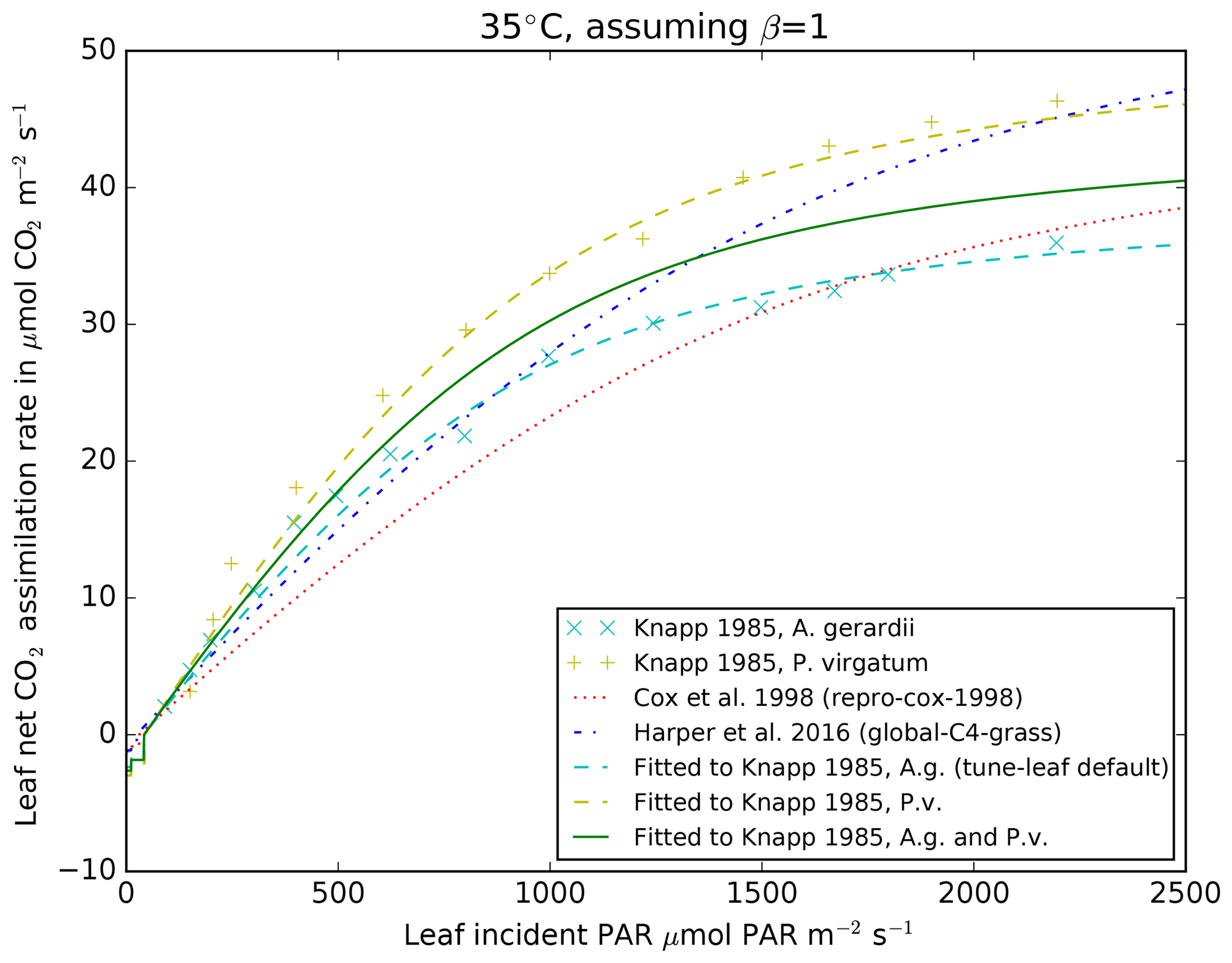
Figure 3Mean observations from Fig. 1 in Knapp (1985) from the
burned plot, early season (May–June 1983) for A. gerardii (cyan
diagonal crosses) and P. virgatum (yellow vertical crosses) for net
CO2 assimilation rate against incident PAR, at 35±2 ∘C. JULES parameters are fitted to the A. gerardii
observations (cyan dashed line), P. virgatum (yellow dashed line)
and a combination of both (green solid line). Also shown are the relations
from the repro-cox-1998 (red dotted line) and
global-C4-grass runs (blue dot-dashed line) at 35 ∘C.
Fitted lines assume no water stress (i.e. β=1) and
ci=200 µ mol CO2 (mol air)−1. Model
lines have been created using the Leaf Simulator package, which reproduces
the internal JULES calculations.
Knapp (1985) also investigated the temperature dependence of net
leaf photosynthesis by artificially altering the temperature of leaves of
A. gerardii and P. virgatum. Their observations showed that the
peaks in both species occurred at approximately the same temperatures but
that the peak was significantly broader in A. gerardii than P. virgatum. In JULES, the temperature dependence of net leaf assimilation for
C4 plants is introduced through a temperature-dependent parameterisation of
the maximum rate of carboxylation of RuBisCO, Vcmax. This enters the
calculation of both the gross rate of photosynthesis and the dark leaf
respiration Rd (since model Rd is proportional to model Vcmax).
Therefore, we can use the relation between net leaf assimilation and
temperature presented in Knapp (1985) to calibrate the JULES
parameters governing the temperature dependence of Vcmax in the model.
The result is illustrated in Fig. 4, alongside the
parameterisations used in the repro-cox-1998 and
global-C4-grass runs. The lines calibrated to the
Knapp (1985) observations peak at approximately 38 ∘C,
whereas the repro-cox-1998 and global-C4-grass
parameterisations peak at approximately 32 and 41 ∘C,
respectively. This leads to very different model behaviour in the temperature
range 32–42 ∘C, where the repro-cox-1998 parameterisation
shows a dramatic decline in Vcmax, which contrasts sharply with the
increase shown in the global-C4-grass parameterisation and the more
stable lines calibrated to the Knapp (1985) observations. Note also
that Polley et al. (1992) found “no apparent relationship” between leaf
temperature and net leaf carbon assimilation in measurements of A. gerardii, S. nutans and P. virgatum, taken at ambient
temperatures between 24.1 and 47.8 ∘C. They speculate
that the difference between their results and the temperature relations found
by Knapp (1985) is due to seasonal acclimatisation.
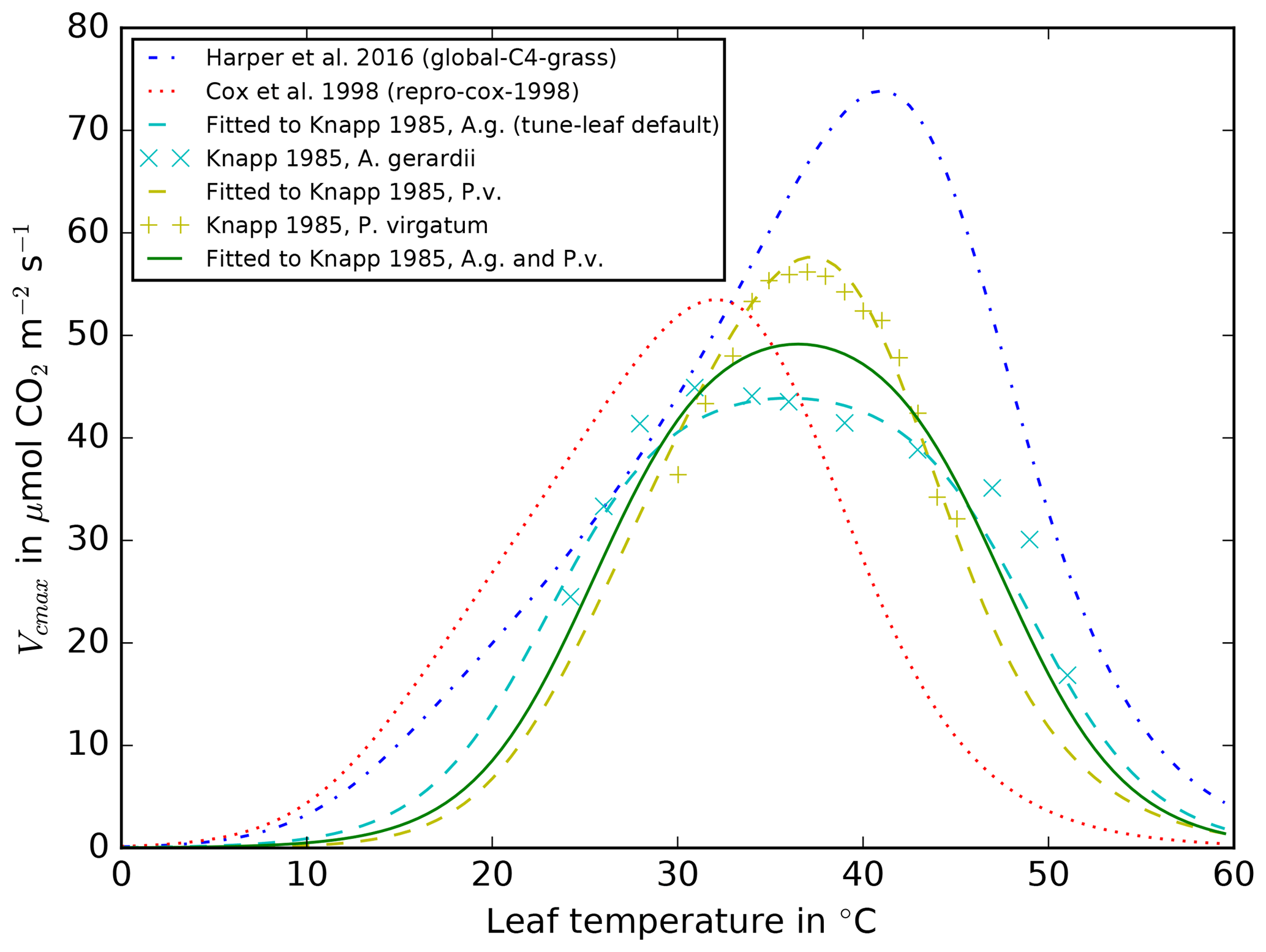
Figure 4Vcmax against leaf temperature for A. gerardii
(cyan diagonal crosses) and P. virgatum (yellow vertical crosses),
using the normalised observations from Fig. 2 in Knapp (1985),
scaled using the fitted light response curves of A. gerardii and
P. virgatum at 35 ∘C shown in Fig. 3. JULES
parameters are fitted to these derived A. gerardii observations
(cyan dashed line) and P. virgatum observations (yellow dashed
line) and a combination of both (green solid line). Also shown are the
relations from the repro-cox-1998 (red dotted line) and
global-C4-grass runs (blue dot-dashed line). Model lines have been
created using the Leaf Simulator package.
As already stated, for the tune-leaf configuration, we use JULES
parameters fit to the A. gerardii data from Knapp (1985),
since A. gerardii is the dominant species at this site. However, to
investigate the uncertainty introduced by the variation between species, we
repeat the runs using parameters fitted to the approximate midpoint of A. gerardii and P. virgatum light response curves and Vcmax
temperature relations. We would expect the best parameter set to lie
between these two parameterisations. However, note that
Knapp (1985) does not have data for Sorghastrum nutans, the
second-most dominant plant species at FIFE site 4439, so we were not able to
take this species into account in this part of the calibration.
It should also be noted that Knapp (1985) reported a drop in the ratio of leaf nitrogen to leaf dry mass over the course of the 1982 season of more than 50 % in the burned plots. This could be a contributing factor to the drop in leaf assimilation they observed over the course of 1983. We were not able to incorporate a time-varying ratio of leaf nitrogen to leaf dry mass into our simulations, which could lead to an overestimation of leaf assimilation in the senescence period.
There were also gas exchange measurements on individual leaves of A. gerardii, S. nutans and P. virgatum taken as part of the FIFE intensive field campaigns in 1987 (Polley et al., 1992). These observations were taken on upper canopy leaves perpendicular to the direct beam of the Sun, with varying absorbed PAR and internal CO2 concentrations (FIFE_PHO_LEAF_46). This includes observations taken before, during and after the dry spell. Therefore, if we are to use these observations to calibrate the unstressed model parameters, we have to process them in such as way as to minimise the influence of the parameterisation of water stress in the model.
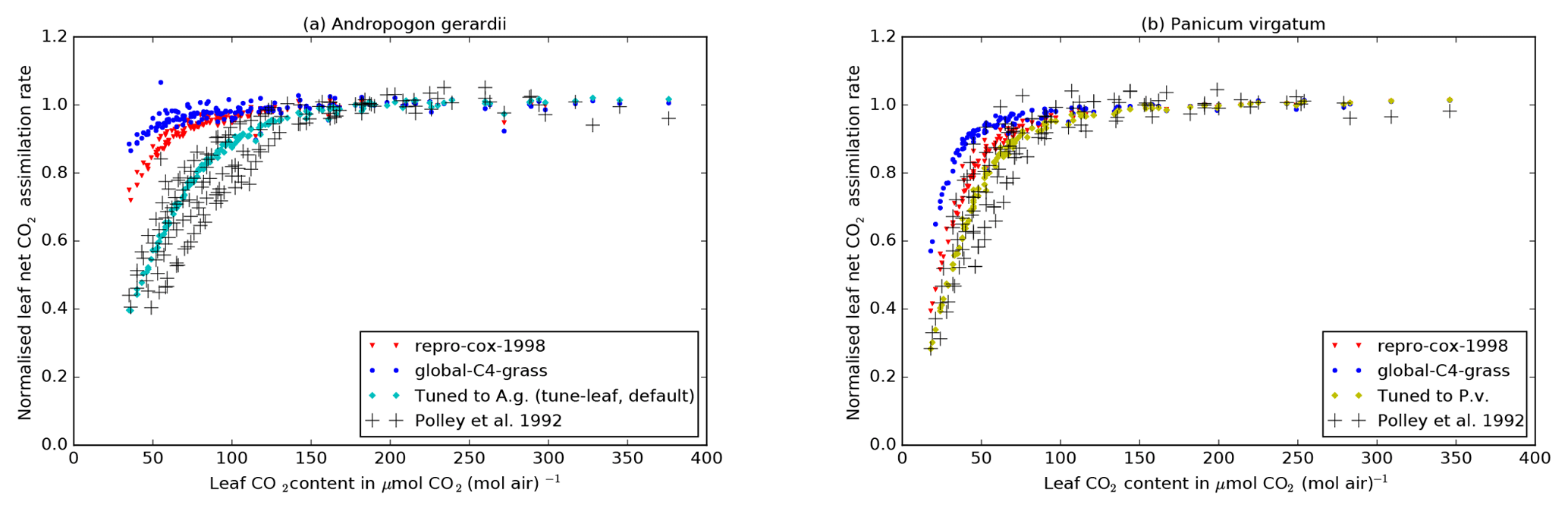
Figure 5Black crosses: Al–ci curves for
Andropogon gerardii (left) and Panicum virgatum (right)
from FIFE_PHO_LEAF_46 (Polley et al., 1992), normalised by the mean
Al of the data points with
ci>150 µmol CO2 (mol air)−1 in that
curve. Only curves with mean incident PAR greater than
1200 µmol PAR m−2 s−1 have been used. Coloured points:
normalised Al calculated from observed ci and
incident PAR for each data point in the curve and the mean Tleaf
observation for each curve, using the JULES relations. The JULES parameters
are taken from the repro-cox-1998 configuration (red triangles), the
global-C4-grass configuration (blue circles) and fits to A. g. data
(tune-leaf default configuration; cyan diamonds) and P. v. data
(yellow diamonds). Model points have been calculated using the Leaf Simulator
package.
To achieve this, we identified individual net leaf assimilation (Al) versus leaf internal CO2 concentration (ci) curves from the FIFE_PHO_LEAF_46 dataset for A. gerardii and P. virgatum (using the observation time and leaf area). We normalised each Al–ci curve using the mean Al for ci>150 µmol CO2 (mol air)−1 for that curve. We then selected Al–ci curves with mean incident radiation greater than 1200 µmol PAR m−2 s−1. This procedure minimises the dependence on water stress or individual leaf nitrogen levels, since these factors approximately cancel out in the relations used internally in JULES when they are manipulated in this way. We can then use these normalised curves to calibrate the model Al–ci response at low ci. For A. gerardii and, to a lesser extent, P. virgatum, this leads to a decrease in the initial slope of the Al–ci curve (Fig. 5).
We also attempted to use the Al–ci curves identified in the FIFE_PHO_LEAF_46 dataset to calibrate the parameters in the JULES relationship between internal leaf CO2 concentration and external CO2 concentration ca. Each individual Al–ci curve was taken at approximately constant humidity, and ca is also provided for each point on the curve. JULES uses the Jacobs (1994) parameterisation:
where Γ is the photorespiration compensation point (Γ=0 for C4), and dq is specific humidity deficit at the leaf surface. f0 and dqcrit are plant-dependent parameters: f0 is a scaling factor on ci and dqcrit governs the strength of humidity dependence of ci. This parameterisation predicts that plotting ci against ca at constant humidity would give a straight line, with gradient . However, when plotting observations from FIFE_PHO_LEAF_46, we found that the slope of the ci:ca ratio changed as ca increased (see Fig. S8 in the Supplement). Therefore, we were unable to calibrate the JULES ci:ca ratio to these data.

Figure 6Ratio of internal to external CO2 against specific
humidity deficit dq. Crosses are derived from leaf measurements of
Andropogon gerardii (cyan) and other C4 grasses (black), taken
in the Konza Prairie (Jesse Nippert and Troy Ocheltree, published in
Lin et al., 2015). Straight lines show the Jacobs model for C4
plants, i.e. . Red dotted
line: repro-cox-1998; blue dot-dashed line:
global-C4-grass; green solid line: tune-leaf. Green dashed
lines: varying dqcrit and setting f0 to the best fit
to the Lin et al. (2015) data for this dqcrit.
Black dotted lines: Medlyn model using ,
, , where
is the value of the Medlyn model parameter
g1 fitted in Lin et al. (2015) to their Konza Prairie
C4 grass measurements. The green solid line (the tune-leaf
configuration) is a good approximation to the Medlyn model with
(because they have both been fit to
the same dataset). The green dot-dashed and green dotted lines have been
tuned to be close to the Medlyn model lines with
and
,
respectively.
Instead, we use leaf measurements of C4 grass in the Konza Prairie, collected in 2008 and published as part of Lin et al. (2015). These were taken at ambient CO2 levels, under unstressed conditions. We can derive the ci:ca ratio from the supplied stomatal conductance, net assimilation and internal CO2 observations, and plot this against specific humidity deficit at the leaf surface, calculated from chamber vapour pressure deficit (VPD), neglecting the effect of the leaf boundary layer (Fig. 6). We calibrate the Jacobs model parameters f0 and dqcrit to these data (green solid line). Given the large scatter of the data and resulting poor fit (R2=0.04), we will also explore the effect of varying dqcrit (green dashed lines a, b, c). In each case, f0 is set to best fit this dataset for this dqcrit (the parameter values are given in Table A3).
Both Knapp (1985) and Polley et al. (1992) found that leaf stomatal conductance gs is proportional to the net leaf assimilation at this site. Their results are approximately consistent with the Lin et al. (2015) observations, given the difference in ambient CO2 levels and the weak dependence on VPD.
As discussed above, in JULES, dark leaf respiration Rd is calculated from
model Vcmax, scaled by a constant. For the tune-leaf
simulation, we tune this constant such that the model dark leaf respiration
at 30 ∘C matches the dark leaf respiration from
Polley et al. (1992) at 30 ∘C (Fig. 7). This is
roughly double the dark leaf respiration at 30 ∘C in the
repro-cox-1998 and global-C4-grass configurations. The
Polley et al. (1992) relation was fitted to observations made at leaf
temperatures of approximately 14–46 ∘C. While our tuned model
parameterisation of dark leaf respiration compares reasonably well in the
range 25–35 ∘C, it rapidly diverges from the Polley et al. (1992)
observations beyond this range. This is particularly true for the higher
temperature values, where the observations in Polley et al. (1992) show an
increase with temperature, whereas the tune-leaf JULES configuration
shows a decrease.
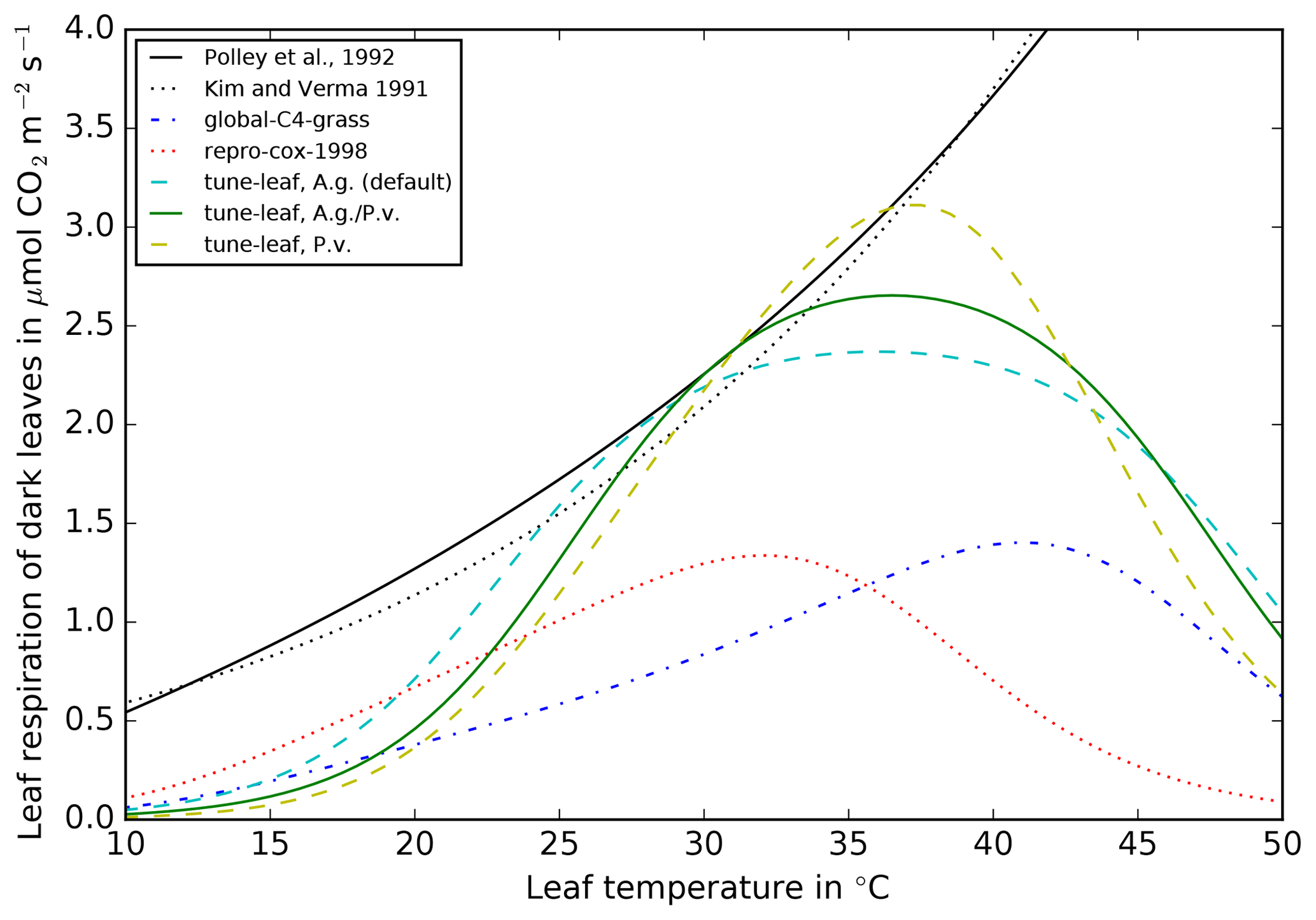
Figure 7Comparison of leaf dark respiration against leaf temperature
relations from Polley et al. (1992) (black solid line)
Kim and Verma (1991a) (black dotted line), repro-cox-1998 (red
dotted line), global-C4-grass (blue dot-dashed line), tuned to A. g.
(cyan dashed line), tuned to P. v. (yellow dashed line) and tuned to both A. g.
and P. v. (green solid line). All lines assume no light inhibition of
respiration. All JULES lines are top of the canopy (TOC) values without water
stress. The lines that reproduce JULES configurations have been calculated
using the Leaf Simulator package.
Polley et al. (1992) found no significant difference between A. gerardii, S. nutans and P. virgatum for a variety of leaf properties: net leaf assimilation under ambient conditions, maximum assimilation under high light and CO2 saturation, temperature response of net assimilation and relationship between assimilation and stomatal conductance under ambient conditions. This implies that the uncertainty we have introduced by not considering S. nutans data throughout most of this calibration is relatively minor.
2.3.2 Onset of water stress and relationship between water stress and leaf water potential
In this section, we calibrate the parameter governing the onset of soil water
stress in the model, p0. In the repro-cox-1998 and
global-C4-grass simulations, p0 is set to 1, meaning that the
model vegetation starts to experience soil water stress at a volumetric soil
moisture m3 m−3 (Fig. 1). This leads to a soil moisture stress factor β
of 0.75–0.55 during the first 10 days of June 1987, i.e. a reduction of
25–45 % compared to the case where model vegetation is not limited by water
availability (Fig. 2).
We can investigate this in more detail using leaf water potential observations as an indicator of the stress levels of the vegetation. Leaf water potential is affected by both the soil water content and the atmospheric water content, as well as other factors affecting transpiration. Both Polley et al. (1992) and Knapp (1985) found a relationship between leaf water potential and net leaf assimilation in their measurements of grasses in the FIFE study area. Polley et al. (1992) measured leaves of A. gerardii and S. nutans throughout the 1988 growing season. These observations showed a drop in net leaf carbon assimilation as the leaf water potential declined through the season: leaf water potentials from −0.34 to −1.5 MPa were consistent with net leaf carbon assimilation rates of 16.2 to 41.5 µmol m2 s−1, whereas lower leaf water potentials of −1.5 to −2.45 MPa were consistent with lower rates of 3.9 to 15.5 µmol m2 s−1 (at internal CO2 concentrations of 200 µmol mol−1 and absorbed PAR of 1600 µmol absorbed quanta m2 s−1). Knapp (1985) carried out weekly leaf water potential measurements of A. gerardii and P. virgatum in 1983 for late May to early October, which showed midday leaf water potential dropping from −0.4 MPa in late May to less than −6.6 MPa (the pressure chamber limit) at the end of July. During this period, net leaf assimilation dropped from approximately 40 µmol m2 s−1 to less than 10 µmol m2 s−1.
Kim and Verma (1991b) proposed a model which considers the prairie vegetation to be completely unstressed until the leaf water potential drops below −1 MPa. This was partially motivated by the Polley et al. (1992) measurements and evaluated using observations of FIFE site 4439 in 1987, i.e. the same site and time period we use in this study. Kim and Verma (1991a) proposed an alternative water stress model, also based on data in Polley et al. (1992), where both the maximum rate of carboxylation of RuBisCO Vcmax and the maximum rate of carboxylation allowed by electron transport Jmax had a dependence on leaf water potential. According to this parameterisation, a leaf water potential of −0.4 MPa introduces a factor of 0.97 into Vcmax, for example, and a leaf water potential of −0.8 MPa introduces a factor of 0.91.
Midday leaf water potential for A. gerardii in the burned plot was approximately −0.4 MPa during the Knapp (1985) “early season” measurement period. Therefore, according to both the Kim and Verma (1991b) and Kim and Verma (1991a) models, considering this period “unstressed” is a very good approximation (i.e. β=1, to within 3 %) and agrees with their statement that “water was not limiting” the vegetation during this period. This validates our use of the Knapp (1985) dataset to tune the “unstressed” JULES parameters in the previous section.
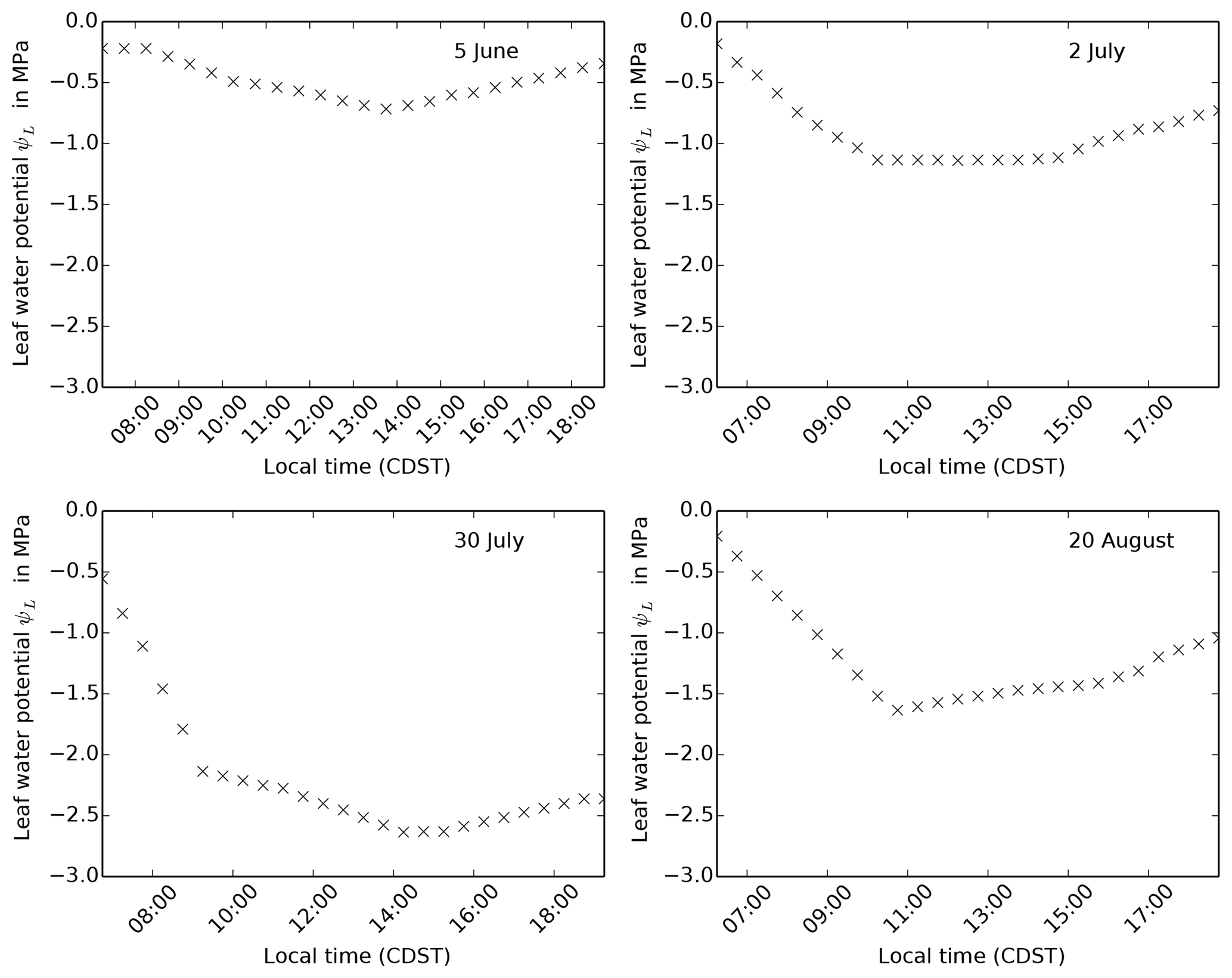
Figure 8Leaf water potential observations for 4 days taken at FIFE site 4439 in 1987, published in Kim and Verma (1991a).
We can now use the same arguments to determine how much water stress the
vegetation should be experiencing at the beginning of June in our runs at
FIFE site 4439 in 1987. Kim and Verma (1991a) present hourly leaf water
potential measurements for A. gerardii leaves at this site, for a
selection of days in 1987 (Fig. 8). On 5 June 1987, they
measured a minimum leaf water potential of approximately −0.8 MPa at 14:00 LT.
According to the Kim and Verma (1991b) model, vegetation at
this leaf water potential would not be water stressed, and according to the
Kim and Verma (1991a) model, Vcmax would be reduced by approximately
9 %. This contrasts sharply with the reduction in net assimilation throughout
the day of 39 %, due to water stress (i.e. β=0.61), experienced in both
the repro-cox-1998 and global-C4-grass simulations on this
day.
For the tune-leaf configuration, we therefore reduce the early
season water stress, to be more consistent with Kim and Verma (1991a) and
Kim and Verma (1991b). This can be achieved by introducing a non-zero
p0 value in the stress factor β. This reduces the soil moisture
threshold at which the plant becomes completely unstressed (β=1) from
θcrit to , as
illustrated in Fig. 1. Assuming that the stress
factor β is 0.9 on 5 June 1987 leads to p0=0.3. The effect of
different values of p0 will be shown in more detail in Sect. 3.
We now examine whether any previous modelling studies at this site support or conflict with this reduction in the soil moisture threshold at which the plant becomes completely unstressed. Crucially, the maximum soil moisture stress factor considered in the original Cox et al. (1998) study was 0.7; therefore, a setup with a p0 of and parameters re-tuned to give a 30 % reduction in unstressed net leaf assimilation would have given the same fit to the data. Similarly, a stress function with p0=0.3 fits the plot of the ratio of actual to potential evapotranspiration to available water in Verma et al. (1992) (when corrected for their different soil properties) at least as well as a stress function with p0=0. An increase in p0 can also be considered a proxy for decreasing θcrit (which, as we have already noted, has a large uncertainty; see Sect. A4). A p0 of 0.2, for example, can be used to mimic the impact of changing θcrit from 0.387, as used in this study and in Cox et al. (1998), to 0.348, as used in Verma et al. (1992).
Kim and Verma (1991a) present hourly water potential measurement of A. gerardii leaves at FIFE site 4439 for 3 other days (in addition to 5 June 1987): 2 July (peak growth period), 30 July (dry period) and 20 August 1987 (early senescence). These show a minimum of −1.2, −2.6 and −1.7 MPa, respectively (Fig. 8). Given the relationships between leaf water potential and net leaf assimilation described above, these leaf water potential measurements imply a drop in leaf assimilation during the middle of the day in the dry period. In contrast, Polley et al. (1992) found “no evident seasonal trend” in the maximum leaf assimilation rate or carboxylation efficiency, despite taking observations throughout the day before, during and after the dry spell in 19871. We were unable to reconcile these results satisfactorily using the associated data in the FIFE_PHO_LEAF_46 dataset (chamber vapour pressure, leaf and chamber CO2 concentrations, leaf and chamber temperatures).
2.3.3 Canopy and optical properties
For the tune-leaf configuration, we keep the values of leaf
reflectance and transmittance from global-C4-grass, as they are
consistent with those measured by Walter-Shea et al. (1992) in 1988
and 1989 as part of the FIFE experiment. Walter-Shea et al. (1992)
found that leaf optical properties were not dependent on leaf water potential
in the range −0.5 to −3.0 MPa.
Leaf angle distribution measurements were taken as part of the FIFE campaign
(SE-590_Leaf_Data) and tended towards
erectophile (Privette, 1996). However, erectophile leaf angle
distributions cannot currently be set in JULES, so we continue to use a
spherical angle distribution, as in the global-C4-grass run.
Walter-Shea et al. (1992) noted that the leaf angle distribution of
grass at FIFE site 4439 was affected by water availability: they concluded
that severe water stress in 1988 probably contributed to a more vertical leaf
orientation in 1988 than in 1989. The uniformity of the canopy in JULES can
be parameterised by a canopy structure factor a (a=1 indicates a
completely uniform canopy; a<1 indicates clumping). It is difficult to get
a numerical estimate of how uniform the canopy is at FIFE site 4439 because
of the large uncertainties in LAI measurements, which we discuss in Sect. A2. However, using LAI from Stewart and Verma (1992), together
with FIFE observations of the fraction of absorbed photosynthetically active
radiation (LB_UNL_42) on a day with mostly diffuse radiation (7 August
1987), gives a rough estimate for a canopy structure factor of 0.8. The
structure factor changes the effective LAI seen by the model radiation
scheme and thus can be used to investigate the effects of the uncertainty in
the LAI dataset.
Leaves of A. gerardii roll (fold) in response to water stress, which reduces their sunlit area while still allowing photosynthesis to continue (Knapp, 1985). This dynamic response of the leaves to drought conditions could be an important factor in modelling canopy photosynthesis during dry spells. However, this behaviour is not implemented in the current version of JULES.
2.3.4 Summary of tune-leaf configuration
The tune-leaf configuration contains parameters that are, in theory,
more appropriate to the tallgrass prairie vegetation at this site, by tuning
the underlying model processes to leaf and canopy measurements taken in the
FIFE study area. The response of leaf photosynthesis to light, CO2 and,
particularly, temperature has been fitted to observations. We note that
previous studies have indicated a relationship between leaf water potential
and net leaf assimilation observations at this site, and that leaf water
potential can be considered an indication of the water stress that the
vegetation is experiencing. While JULES does not model leaf water potential
explicitly, a review of the available leaf water potential observation
measurements indicates the need to delay the onset of model water stress in
this tuned configuration, compared to the repro-cox-1998 and
global-C4-grass configurations, which we achieve through setting a
non-zero p0 parameter. We note that there remains significant uncertainty
in the threshold for the onset of water stress, the calculation of internal
CO2 concentration and the uniformity of the canopy. There is also an
uncertainty introduced by interspecies variation. We note that the
comparison with observations has revealed some possible limitations of the
model, such as the fixed leaf nitrogen content and leaf orientation
(spherical) through the season and an absence of leaf folding.
Figures 9, 10 and 11 show the model output for gross primary productivity (GPP), net canopy assimilation and latent heat flux for 8 days during 1987. These dates sample a range of different vegetation states: 5 June is in the early growth stage, 2 and 11 July are in the peak growth stage, 23 July, 30 July and 11 August are in the dry period, and 17 and 20 August are in the early senescence period (Verma et al., 1992). All of these dates comply with the selection criteria described in Cox et al. (1998) (following Stewart and Verma, 1992). Days with, or directly after, significant rainfall have been avoided, in order to reduce the effect of evaporation from the canopy surface and bare soil. The model latent heat flux is compared to latent heat flux measurements in the FIFE_SF30_ECV_33 dataset. GPP and net canopy assimilation are derived from CO2 flux measurements in FIFE_SF30_ECV_33, using the method in Cox et al. (1998). Further net canopy assimilation estimates have also been read from Kim and Verma (1991a) (see Sect. A7 for more information).
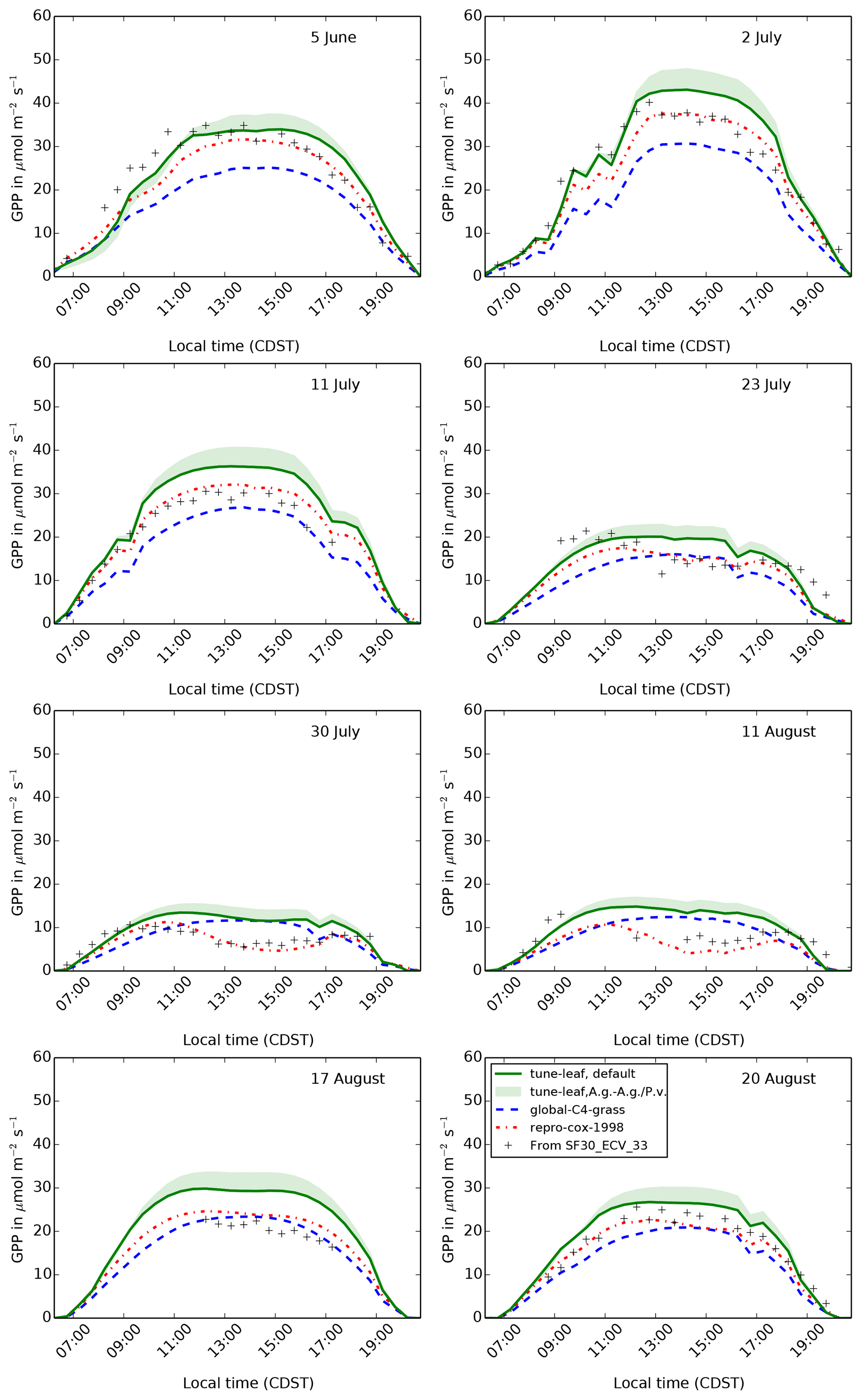
Figure 9The diurnal cycle of GPP at site 4439 in the FIFE area for 8 days in 1987: 5 June (early growth), 2 and 11 July (peak growth), 23 July, 30 July and 11 August (dry period), and 17 and 20 August (early senescence). Green band shows uncertainty from fitting plant parameters to A. gerardii compared to fitting to both A. gerardii and P. virgatum.
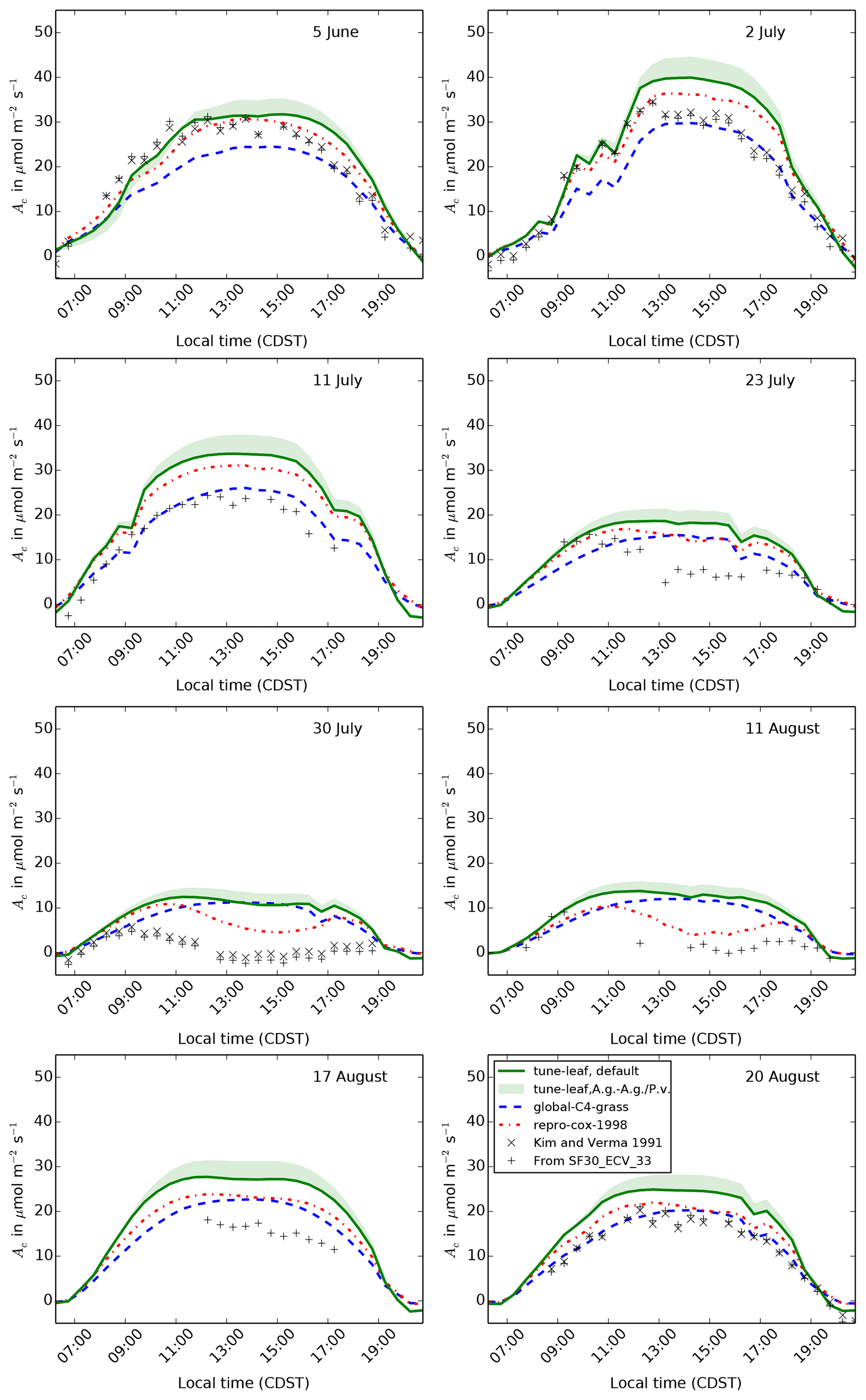
Figure 10The diurnal cycle of net canopy assimilation Ac at site 4439 in the FIFE area for 8 days in 1987: 5 June (early growth), 2 and 11 July (peak growth), 23 July, 30 July and 11 August (dry period), and 17 and 20 August (early senescence). Green band shows uncertainty from fitting plant parameters to A. gerardii compared to fitting to both A. gerardii and P. virgatum.
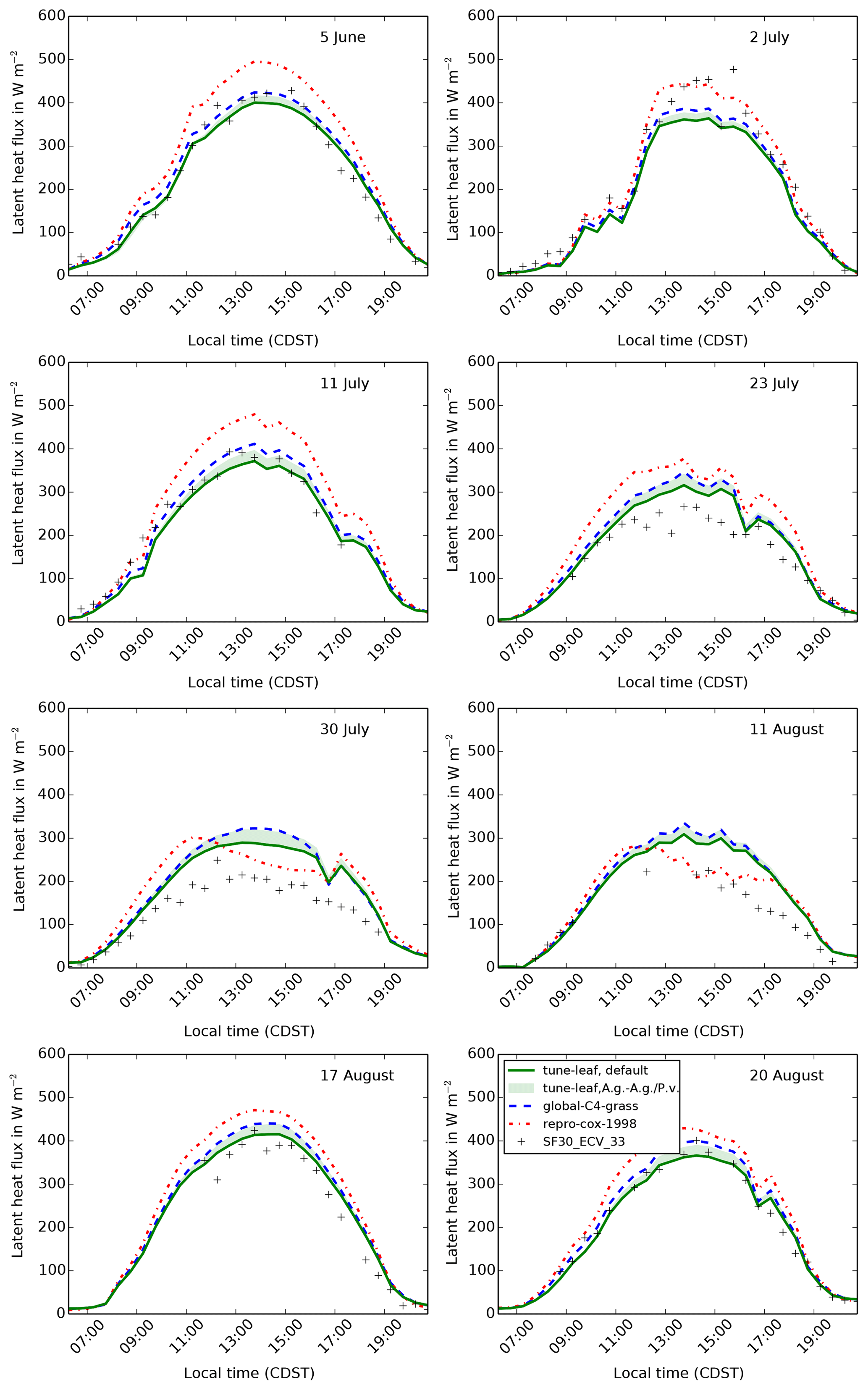
Figure 11The diurnal cycle of latent heat flux at site 4439 in the FIFE area
for 8 days in 1987: 5 June (early growth), 2 and 11 July (peak growth),
23 July, 30 July and 11 August (dry period), and 17 and 20 August (early
senescence). Green band shows uncertainty from fitting plant parameters to
A. gerardii compared to fitting to both A. gerardii and
P. virgatum (upper limit corresponds to the combined A. g., P. v. fit, lower limit to the A. g. fit (i.e. the default
tune-leaf configuration).
3.1 repro-cox-1998 and global-C4-grass simulations
GPP in the repro-cox-1998 simulation after 10:00 LT compares
very well to GPP derived from the flux tower data (Fig. 9), for all growth stages. This is expected, given that
this simulation is designed to reproduce the model from Cox et al. (1998),
which was tuned to this flux dataset. The global-C4-grass simulation
reproduces the carbon fluxes reasonably well outside the dry period, although
GPP is underestimated during the growth stages. For example, GPP is
underestimated by approximately 30 % during the middle of the day on 5 June. During the dry period, however, the global-C4-grass simulation
poorly captures the early morning peak and subsequent decline in GPP
indicated by the carbon flux observations. The repro-cox-1998 run
captures this behaviour through its response to leaf temperature. The diurnal
cycle of air temperature on these days is shown in Fig. S5 and modelled
leaf temperature in Fig. S6. Recall that Vcmax in the
repro-cox-1998 simulation declines at leaf temperatures above
32 ∘C. This causes a decline in modelled carbon assimilation during
the hottest parts of the day (this is demonstrated explicitly in additional
runs in the Supplement). However, as discussed in Sect. 2, the temperature response in the repro-cox-1998
configuration is not supported by observations in Knapp (1985) or
Polley et al. (1992). Therefore, it appears that, while the model is
successfully capturing the shape of diurnal cycle during the dry period, it
is not achieving this with the correct physical process.
Similarly, net canopy assimilation in the repro-cox-1998 simulation
compares well to the time series derived from the flux tower observations,
although it has lower leaf respiration, particularly on 23 and 30 July (Fig. 10). As discussed in Sect. A7, the leaf respiration values assumed when processing
the flux measurements were based on observations of leaf respiration in
Polley et al. (1992). In Sect. 2.3, we showed that the
repro-cox-1998 simulation underestimates leaf respiration compared
to the Polley et al. (1992) dataset, particularly at the higher temperatures
experienced during the middle of the day in the dry period. While the
global-C4-grass configuration also simulates lower leaf respiration
values than seen in Polley et al. (1992), a combination of a low bias in the
GPP and a peak in Vcmax at higher temperatures (compared to the
repro-cox-1998 simulation) reduces the impact on net canopy
assimilation.
The latent heat flux is reasonably well modelled in general in both the
repro-cox-1998 and global-C4-grass simulations outside the
dry period (errors in the peak of the diurnal cycle of less than 20 %).
However, both simulations overestimate the latent heat flux during the dry
period (Fig. 11). This is expected, given that we
have already shown that the canopy carbon assimilation is overestimated, and
stomatal conductance is proportional to the net leaf assimilation in the
model.
3.2 tune-leaf simulations
The tune-leaf configuration generally overestimates both GPP (Fig. 9) and net canopy assimilation (Fig. 10) compared to the observations and the
repro-cox-1998 and global-C4-grass simulations. On days
during the dry period, the tune-leaf simulation behaves
characteristically similarly to the global-C4-grass simulation in
that it also does not capture the midmorning peak and subsequent decline in
GPP and assimilation. When fitting the tune-leaf configuration in
Sect. 2, we highlighted uncertainties in some of the key
parameters, and we will now look at the effect of these in turn.
Firstly, the tune-leaf configuration is based on observations of the
dominant grass species at this site, A. gerardii. In Sect. 2, we also fitted parameters to another grass species at this
site: P. virgatum and a “combined” set fitted to both species. Since
A. gerardii is almost twice as abundant at this site in 1987 as P. virgatum, and in the absence of parameter fits to the other grass species at
this site, we would estimate that the most representative parameters lie
somewhere between these two parameter sets. Using this combined A. g./P. v. parameter set increases GPP and net canopy assimilation on the
order of roughly 10 % compared to using the set fitted solely to A. g.
(Figs. 9, 10), from which we
conclude that the error introduced from using the dominant grass species is
relatively minor.
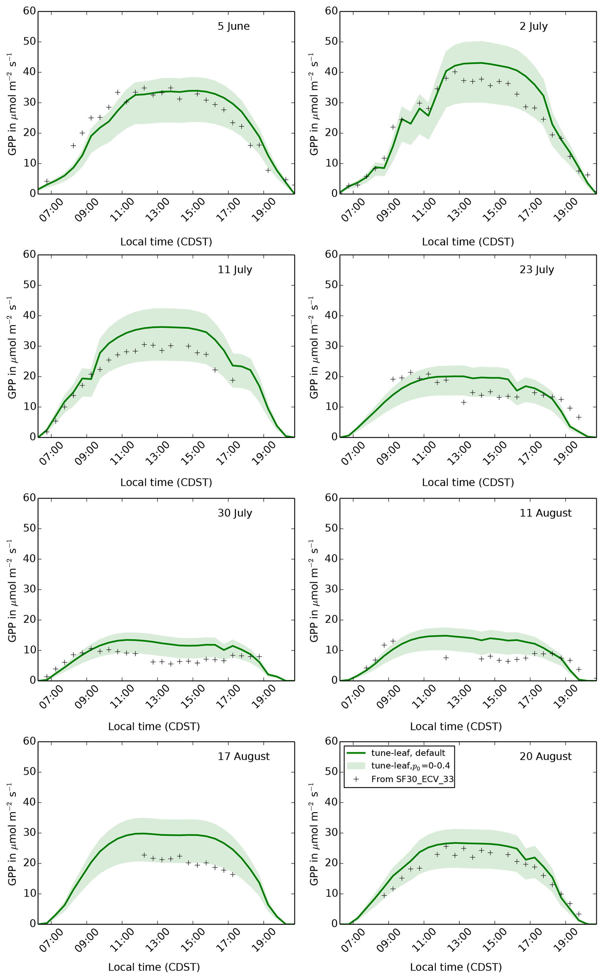
Figure 12The diurnal cycle of GPP at site 4439 in the FIFE area for 8 days in
1987: 5 June (early growth), 2 and 11 July (peak growth), 23 July, 30 July
and 11 August (dry period), and 17 and 20 August (early senescence). Green
band shows how the tune-leaf simulation would vary for p0 in the
range 0 to 0.4 (lower limit corresponds to p0=0, upper limit to
p0=0.4).
A key difference between the tune-leaf configuration and the other
configurations is the introduction of a non-zero p0. Figure 12 illustrates that varying p0 from 0 (as in
the repro-cox-1998 and global-C4-grass simulations) to 0.4
has a strong effect on GPP, as expected. It demonstrates the importance of
ensuring that the threshold for water stress is consistent with the
“unstressed” leaf observations we calibrated against. Continuing to use
p0=0 with the newly tuned unstressed parameters would have resulted in
much-too-low GPP during the early growth period. Recall also that changing
p0 can be considered a proxy for changing the critical soil moisture.
Therefore, these runs also demonstrate the sensitivity to uncertainty in the
soil properties.
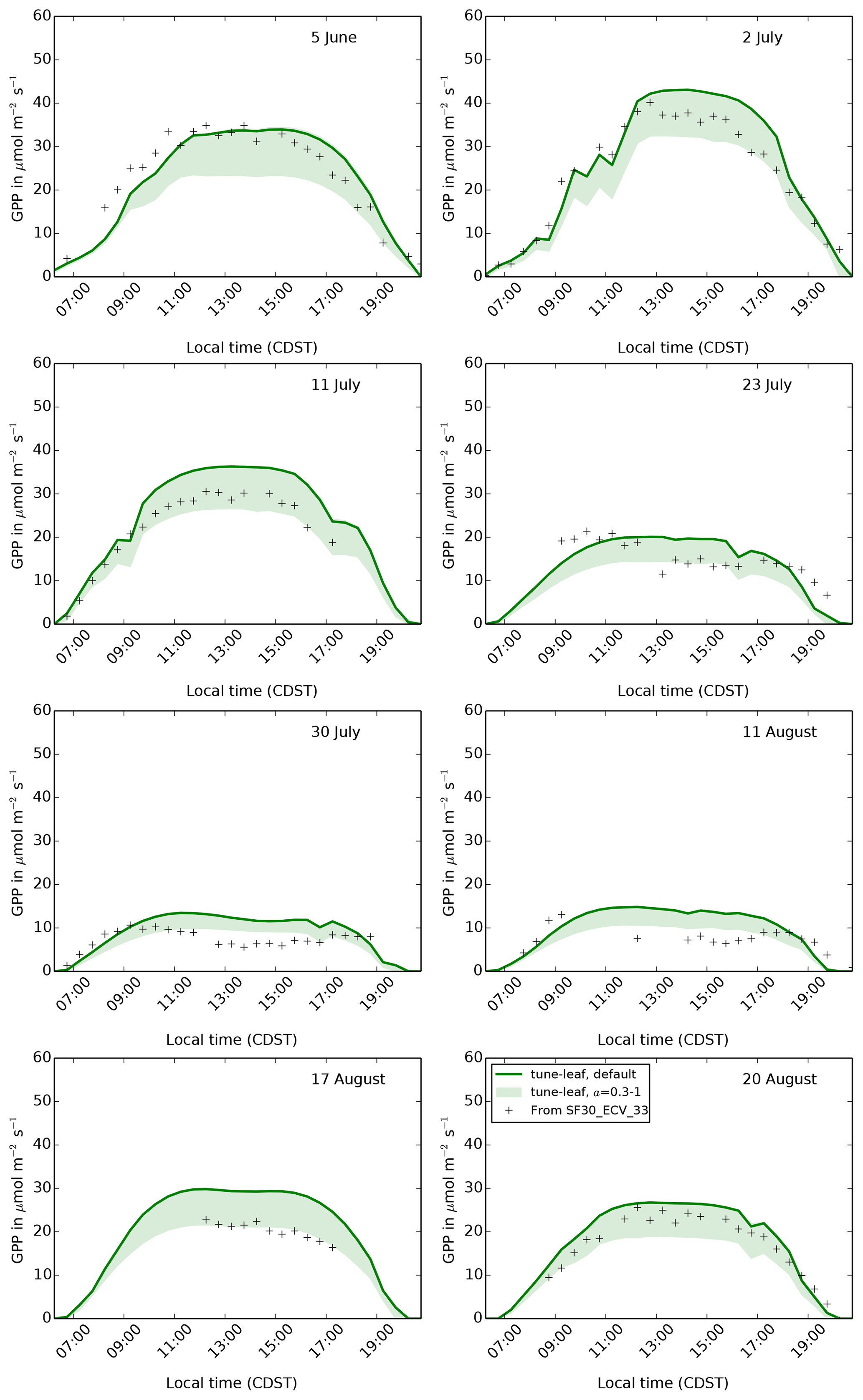
Figure 13The diurnal cycle of GPP at site 4439 in the FIFE area for 8 days in
1987: 5 June (early growth), 2 and 11 July (peak growth), 23 July, 30 July
and 11 August (dry period), and 17 and 20 August (early senescence). Green
band shows how the tune-leaf simulation would vary for a canopy
structure factor a in the range 0.3 to 1 (upper limit corresponds to a=1,
lower limit to a=0.3).
The effect of varying the canopy structure factor on GPP can be seen in Fig. 13. This can also be seen as a proxy for examining the effect of reducing LAI as it changes the effective LAI seen by the model radiation scheme. Varying the canopy structure factor in the range 0.8–1.0 has a negligible effect on GPP on these days. However, reducing the canopy structure factor from 0.8 to 0.3 has a large negative impact on GPP. As discussed in Sect. 2, this range is inside the error given in the LAI dataset documentation. The error in LAI for this site therefore has a large impact on the modelled canopy carbon fluxes.
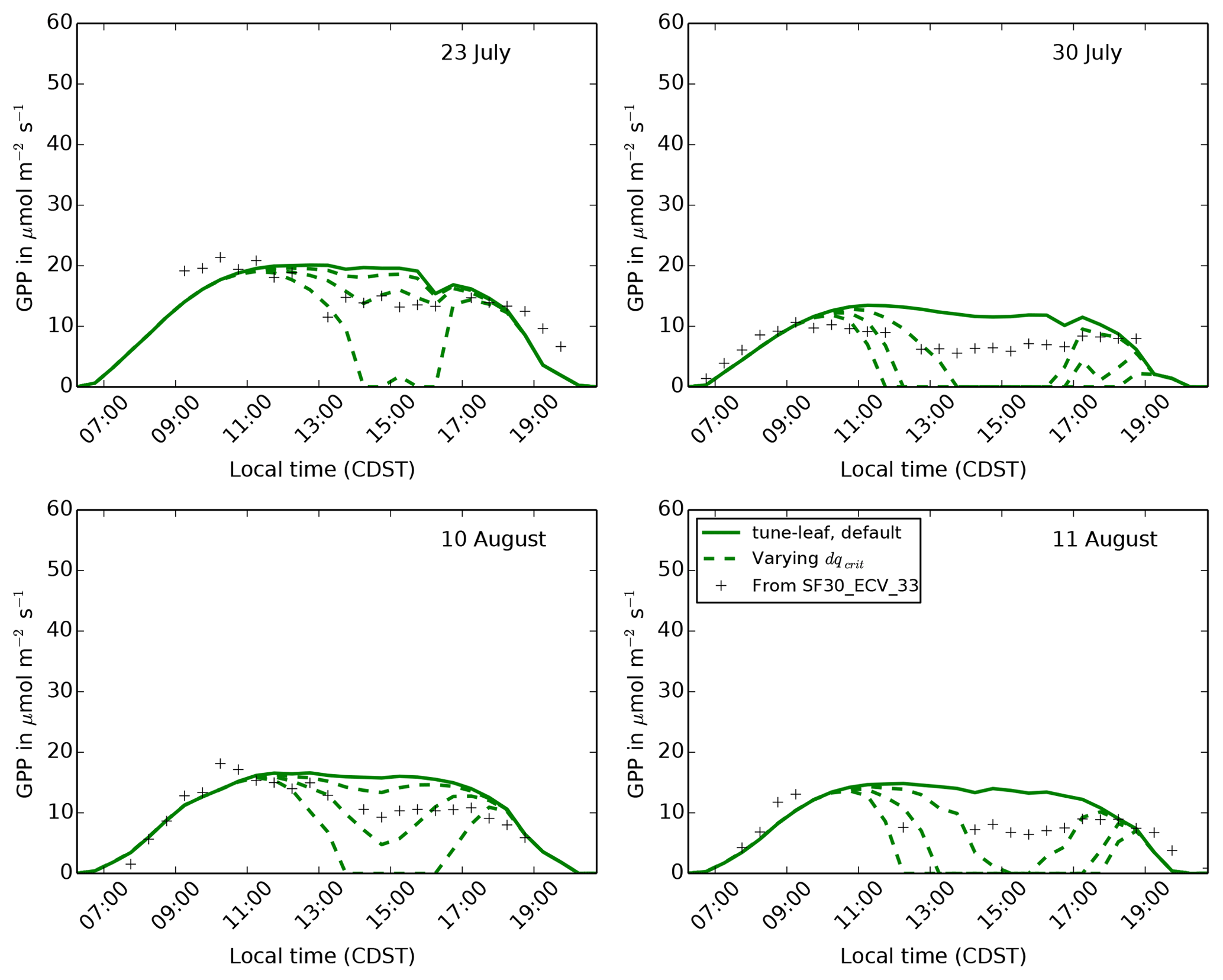
Figure 14The diurnal cycle of GPP at site 4439 in the FIFE area for 4 days in
during the dry period of 1987. Solid green lines use the tune-leaf
configuration. Dashed dashed green lines show how GPP varies if
dqcrit is increased, while f0 is changed to maintain
the best fit to the Konza Prairie C4 grass observations in
Lin et al. (2015) (upper, middle and lower dashed lines correspond to
parameter combinations a, b and c, respectively, as defined in
Table A3).
Less straightforward to investigate is the effect of the uncertainty in the calibration of the JULES ci humidity response. Recall that the observational dataset used in Sect. 2 had a large spread in ci compared to its range of specific humidity deficit values. This made it difficult to tune the parameter dqcrit separately to the overall scaling factor f0. We therefore take the approach of systematically varying dqcrit (while setting f0 to keep the best fit to the observations in Fig. 6), to show qualitatively that a different humidity calibration cannot improve the agreement with the GPP observations during the dry spell. Figure 14 compares modelled GPP for three different dqcrit, f0 combinations: dqcrit=0.048, f0=0.59 (upper green dashed line), dqcrit=0.040, f0=0.64 (central green dashed line) and dqcrit=0.035, f0=0.68 (lower green dashed line) for 4 days during the dry spell. Plots of specific humidity deficit on these days are given in Fig. S7. None of these parameter combinations are able to fit the steady but low rate of GPP during the middle period of the day: they transition from almost no humidity-induced effect on GPP to a sudden decline. The timing of this decline varies across the 4 days shown. This demonstrates that, while lower ci values in these runs during the day in the dry period can reduce GPP, the magnitude of the slope of ci:ca against dq is too large. These two effects cannot be reconciled while still maintaining consistency with the unstressed observations in Lin et al. (2015). This implies that the Jacobs parameterisation used in JULES, where the relationship between ci:ca and specific humidity deficit does not vary over the course of the run, does not have the flexibility needed to capture the behaviour of GPP at this site.
3.3 What potential model developments could improve the diurnal cycle of JULES GPP at this site?
As we have seen, the global-C4-grass configuration, which is typical
of how this site would be modelled in a global JULES run, is unable to
capture the diurnal cycle of GPP (and also net canopy assimilation and latent
heat flux) at this site during the dry period in 1987. Replacing the generic
C4 grass tile parameters with parameters that are calibrated to observations
taken of vegetation at this particular site (the tune-leaf
configuration) does not improve ability of the model to capture the diurnal
cycle in these fluxes. We have demonstrated that this conclusion is robust to
uncertainties in LAI, soil moisture, leaf parameters, canopy parameters and
soil parameters.
We will now explore a number of possible options for improving the standard
representation of the dry period diurnal GPP cycle at this site. Firstly, the
model diurnal cycle can be greatly improved via the careful selection of
parameters in the existing leaf temperature-dependent calculation of
Vcmax. This was demonstrated in the model runs in Cox et al. (1998),
which we have closely reproduced with the repro-cox-1998
configuration. This method has the advantage that it provides a close fit to
data and does not require any changes to the model code. A disadvantage of
this method is that the Vcmax model parameterisation becomes an
effective parameterisation which no longer has a clear biological
interpretation. It therefore becomes more difficult to constrain from results
in the literature. The numerical success of this method is due to high leaf
temperatures acting as a proxy for high atmospheric demand during the middle
of the day in the dry period (Figs. S6 and S7). While these
temperature parameters provide a good approximation at this site in this
particular year, it does not follow that these same temperature parameter
values would be appropriate for other locations or at this location under a
changing climate.
Secondly, the model could be extended to include a soil moisture effect on the internal leaf CO2 concentration ci. As we demonstrated in Sect. 3, the current expression for ci in JULES cannot simultaneously fit the unstressed observations and be able to reduce ci to the required levels to affect GPP during the dry season without also increasing the strength of the response to specific humidity deficit. This results in the humidity-induced stomatal closure occurring too suddenly on days during the dry period. Introducing a soil moisture dependence in ci would allow ci to be lower on days where soil water was limiting for all humidity levels, while maintaining the higher values on unstressed days. Zhou et al. (2013) and De Kauwe et al. (2015) both achieve this by adding a soil moisture dependence to the VPD term in the Medlyn conductance model (Medlyn et al., 2011). The Medlyn model is based on the theoretical argument that stomata should act to minimise the amount of water used per unit carbon gained, leading to a stomatal conductance , where g0 and g1 are free parameters.
As demonstrated in De Kauwe et al. (2015), the parameters in the Jacobs model
(f0, dqcrit) can be chosen so that the resulting ci:ca ratio
approximates the Medlyn model, for mid-range VPD values. The unstressed Konza
Prairie C4 grass measurements used in Sect. 2 to calibrate
the ci:ca ratio in the tune-leaf configuration were actually
provided in Lin et al. (2015) as part of a comprehensive study to tune
the g1 parameter in the Medlyn model for different vegetation types (with
g0=0). Using the Medlyn model with their calibrated g1 value
() does indeed give a similar ci:ca to our
tune-leaf configuration (Fig. 6, solid green
line).
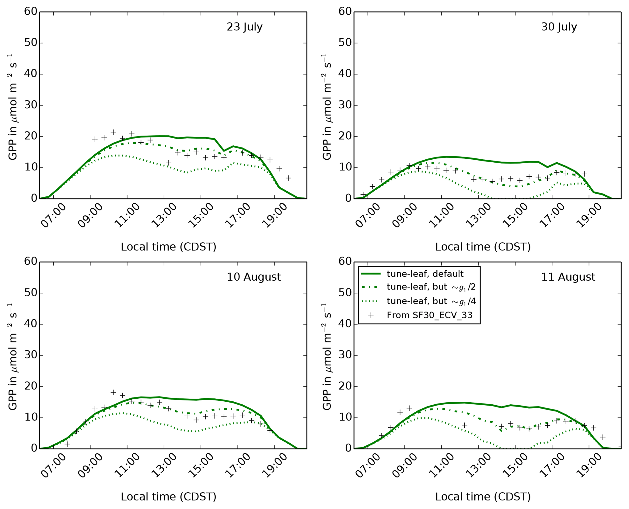
Figure 15The diurnal cycle of GPP at site 4439 in the FIFE area for 4 days in
during the dry period of 1987. Solid green lines use the tune-leaf
configuration. The ci:ca ratio in this
configuration closely corresponds to the ci:ca
ratio for C4 grasses in the Konza Prairie in Lin et al. (2015),
using the Medlyn model and fitting the Medlyn model parameter g1
to measurements taken in 2008
( kPa−0.5). The dot-dashed
lines and dotted lines show the results from fitting the JULES parameters
dqcrit and f0 to approximate the Medlyn model when
and
(the parameter values are given in
Table A3).
Therefore, to investigate the effect of a soil moisture-dependent g1 on GPP, we can set the JULES ci:ca ratio to mimic a lower g1 and try this out on days with low soil moisture. For this test, we choose JULES parameter values that provide a rough approximation to the Medlyn model with and (Fig. 6, dot-dashed and dotted green lines). These reductions in g1 are well within the range observed in Zhou et al. (2013) for a range of different vegetation types under water-limited conditions. The resulting JULES parameter values are given in Table A3. Figure 15 demonstrates that lowering ci:ca in this way is able to qualitatively reproduce the shape of the diurnal cycle of GPP in the dry period. The run mimicking , in particular, is a very good match to the observations. This shows the potential value of extending JULES to allow interaction between the plant response to soil moisture dependence and VPD.
Another way to implement this interaction in JULES would be to add a dependence on leaf water potential, since leaf water potential is affected by both soil moisture (water supply) and VPD (atmospheric water demand). As discussed in Sect. 2.3, there is an observed relationship between leaf water potential and leaf assimilation in grass species at this site.
Previous studies have demonstrated that models with an explicit dependence on leaf water potential can successfully capture the dry period diurnal cycle at this site. Kim and Verma (1991a) were able to qualitatively capture the midmorning peak and subsequent decline in net canopy photosynthesis on 30 July at this site, using a model in which both Vcmax and Jmax had a dependence on their leaf water potential measurements. Furthermore, Kim and Verma (1991b) were able to reproduce this behaviour in canopy conductance at this site on 30 July and 11 August 1987 using a model that included an explicit dependence on observed leaf water potential, in addition to a direct dependence on VPD.
Leaf water potential is not currently modelled explicitly within JULES. Typically, in plant hydraulic models, leaf water potential is calculated assuming a steady-state water balance, using the soil water potential, transpiration, and leaf-to-root and root-to-soil resistance terms (as in, e.g. Newman, 1969). Adding this to the JULES code is technically non-trivial, as water stress is currently applied to leaf-level processes before transpiration is calculated. Also, modelling the plant resistances would require additional input parameters, which would need to be constrained from observations.
Stress parameterisations involving leaf water potential come in a range of complexities. The simplest involve inserting a leaf-water-potential-dependent stress factor into an existing part of the model, e.g. the limiting photosynthesis rates as in Kim and Verma (1991a), or stomatal conductance, as in Kim and Verma (1991b) and Tuzet et al. (2003). More sophisticated models include the plant hydraulics as part of schemes incorporating risk–benefit analysis (e.g. Sperry et al., 2017; Eller et al., 2018) and/or chemical signalling (e.g. Tardieu and Davies, 1992; Dewar, 2002; Huntingford et al., 2015).
Finally, another way to improve the diurnal cycle of GPP in the dry period would be to incorporate a parameterisation of leaf rolling. For example, effective leaf area available to the radiation scheme could be decreased during hot, dry weather. Kim and Verma (1991a) attribute the residual overestimation of net canopy carbon assimilation on days during the dry period of their leaf water potential-based model to this effect. It would therefore be interesting to investigate the contribution that leaf rolling makes to the overall plant water use strategy. However, while the occurrence of leaf rolling/folding at the FIFE site has been recorded, the effect has not been quantified. This would be a necessary first step for modelling this process at this site.
3.4 Can the FIFE dataset make a useful contribution to current-day JULES evaluation and development work?
A global land-surface model such as JULES needs to perform well for a wide range of climate regimes, timescales, spatial scales and vegetation types. Model evaluation or development work needs to represent this variety. The availability of comprehensive databases, such as FLUXNET (Baldocchi et al., 2001) and TRY (Kattge et al., 2011), have revolutionised land-surface science by giving easy access to observations from a wide variety of sources, in a common format. Given this context, why would a modeller consider also using the FIFE dataset?
Firstly, FIFE provides an ideal case study for improving the model representation of water stress on carbon and water fluxes in JULES in tallgrass prairie. While, at one time, tallgrass prairie extended over 10 % of the contiguous United States (Fierer et al., 2013), it has declined 82 %–99 % since the 1830s due to agricultural use (Sampson and Knopf, 1994; Blair et al., 2014a). However, grasslands in general (including other grass- and graminoid-dominated habitats, such as savanna, open and closed shrubland, tundra) cover more terrestrial area than any other single biome type (up to 40 % of Earth's land surface; Blair et al., 2014a). It is therefore important to include lots of examples of grasslands in any global analyses of vegetation responses to changing conditions. The Konza Prairie LTER site, where FIFE was based, has been used extensively to investigate the dynamics and trajectories of change in temperate grassland ecosystems, including drivers such as fire, grazing, climate and nutrient enrichment (see Blair et al., 2014b for a review).
FIFE looked at the processes for representing water stress in detail and intensively studied the relevant factors. This has led to a wide variety of complementary observations and literature specifically focusing on how these data can be used to inform models. LAI is a good illustration of this advantage. As we have discussed, LAI is an important parameter for modelling canopy water and carbon fluxes. LAI was measured by multiple groups at FIFE, directly and indirectly, and the large differences found between the different attempts was fully explored at the time. We can use their results to inform our own use of these datasets.
When adding a new process to a global land-surface model, it is important to tune new parameters to a comprehensive range of datasets. For example, as mentioned in Sect. 3.3, Lin et al. (2015) use data for 314 species from 56 sites across the world to tune the new g1 parameter introduced in the Medlyn model of stomatal conductance for key plant functional types. This breadth of sites and vegetation types is essential. Each site contributed leaf gas exchange observations taken under similar protocols to allow a carefully controlled common analysis.
Access to individual experiments, which have investigated the combined effect of a wide range of processes, such as FIFE, can play a complementary role in land-surface evaluation and development. For example, FIFE provides cases where improving an individual process in isolation degrades overall model performance. As we have shown, calibrating unstressed model Vcmax (T=25 ∘C) from leaf observations without also calibrating when the model is considering the vegetation to be unstressed significantly underestimates early season GPP. Similarly, tuning the model parameters to improve the fit to canopy GPP and evapotranspiration can result in an unrealistic temperature dependence of Vcmax. Looking at sites in a holistic way can also highlight complications or influences that might not a priori have been considered, such as leaf rolling in our case.
There are two main disadvantages to the use of FIFE in evaluation and model development studies. The first is the limited time period: observations are available for a period of up to 3 years, with some key measurements only undertaken during the intensive field campaigns. Where long-term effects are being studied, alternative datasets would need to be used.
The second disadvantage is that it is relatively more time consuming to add FIFE to an evaluation study, compared to adding an extra site from one of the large, standardised databases such as FLUXNET. This is partly because FIFE provides a choice of different datasets to use for forcing, calibrating parameters and evaluation, which takes time to investigate. It is also partly because, although the data are easily downloadable, well documented and in common file formats, they still need to be manipulated into a format that can be used in JULES runs. We aim to address this issue by providing a suite that can be used to preprocess the FIFE data and run JULES with the configurations described in this paper (see the “code and data availability” section).
This aim is central to the provision of this paper. FIFE is the first “JULES golden site”, a concept that was launched at the annual JULES meeting in 2018. A JULES golden site is a site targeted by the JULES community because it can help address one of the key science questions facing JULES and has high-quality observational data that can be used to drive JULES and evaluate the output. It creates a network of researchers within the JULES community with experience of how this site can be exploited for JULES development, with input from site investigators. A key component is the provision of shared runs and evaluation datasets, which can be gradually expanded and improved.
In our study, we have focused on the contribution that FIFE can make to the development of water stress in JULES. This has governed the choices we have made when setting up our configurations, e.g. choosing to prescribe LAI and soil moisture. However, we note here that FIFE could also be used to investigate other processes, such as plant and soil respiration (Sect. A7), the seasonal decline in leaf nitrogen (Knapp, 1985) and the modelled energy balance (Kim and Verma, 1990a; Colello et al., 1998).
In their closing remarks, Sellers and Hall (1992) state that “FIFE created an environment for the discussion of all aspects of the land-surface component of Earth remote sensing and Earth system modelling and provided a dataset which has been and continues to be used to test models and algorithms”. Our study demonstrates that this is still the case, 25 years after this remark and 30 years after the experiment itself. There is a wealth of available data and extensive analysis in the literature, particularly on the response of vegetation carbon and water fluxes to periods of low water availability.
Historically, FIFE observations were used to derive the original soil moisture stress parameterisation in JULES. This early model was extremely successful in fitting the canopy net assimilation and water fluxes, during both dry and wet periods (Cox et al., 1998). However, a typical modern-day configuration of JULES, from Harper et al. (2016), which models the FIFE vegetation with generic C4 grass parameters, could not reproduce the observed diurnal cycle of carbon and water fluxes during the period of low water availability. Calibrating the plant parameters to site observations did not solve this problem, nor could it be explained by the large observational uncertainties in leaf area index, soil moisture and soil properties. Reproducing the original configuration in Cox et al. (1998) illustrated that the temperature dependence of the maximum rate of carboxylation of RuBisCO Vcmax in the model was key for reducing modelled photosynthesis rates during the hottest parts of the day in the dry period, since model Vcmax declined steeply at the leaf temperatures experienced on these days. However, this temperature response was not supported by the available leaf-level gas exchange observations. With a more realistic temperature response, this configuration was no longer able to capture the reduction of photosynthesis during the middle of the day in the dry period either.
FIFE therefore provides a robust example of how the current processes that govern the way that vegetation in JULES responds to water availability do not behave realistically during dry spells for this type of grassland. This deficiency could be addressed by allowing the effect of soil moisture availability and vapour pressure deficit on stomatal conductance to interact, for example, via leaf water potential. FIFE is thus a useful site to consider when evaluating the benefits of new water stress parameterisations to JULES, particularly those with an explicit representation of plant hydraulics.
FIFE can play a role in JULES evaluation and development only as one small component of a comprehensive range of datasets, covering different climate regimes, timescales, spatial scales and vegetation types. FIFE is valuable partly due to the concentration of overlapping datasets. Key observables such as leaf area index, soil moisture and soil properties, from independent investigations during FIFE, have been intensively analysed and yet still show a wide spread. This illustrates the intrinsic variability of these parameters, which must be carefully considered when scaling up to gridded global runs. FIFE also provides clear examples of how calibrating one process to observations can reduce the overall model performance, due to compensating biases (such as calibrating the unstressed parameters without also checking the time period during which the model considers the vegetation to be unstressed). Confidence that the model is capturing key processes is necessary if the model is being run into new regimes, such as when forced with climate projections. This ability to disentangle and evaluate individual processes emphasises the value that intensive experiments such as FIFE have towards the larger modelling community evaluation efforts. In order to facilitate the inclusion of FIFE data in comprehensive model evaluations, this paper is accompanied by a release of the full set of data processing and configuration files needed to reproduce these model simulations. It is intended that this suite of files will continue to develop in the future as additional parts of the model are evaluated against the FIFE dataset, so that the JULES community can build up a comprehensive body of knowledge of data and model runs at this site.
JULES can be downloaded from the JULES FCM repository on the Met Office Science Repository Service at https://code.metoffice.gov.uk/trac/jules (last access: 30 May 2019, registration required). We use JULES version 5.0 (tag “vn5.0”), which corresponds to revision 9522. The Leaf Simulator can be downloaded from https://code.metoffice.gov.uk/trac/utils (last access: 30 May 2019). Where data points have been read directly from published plots, this was done with the EasyNData tool (Uwer, 2007). The three JULES simulations described in this study can be reproduced using the rose suite u-bb181, available at https://code.metoffice.gov.uk/trac/roses-u/browser/b/b/1/8/1/trunk (last access: 30 May 2019). This suite also contains instructions for downloading the driving data from ORNL DAAC and a script to preprocess the driving data, including calculating the diffuse radiation fraction.
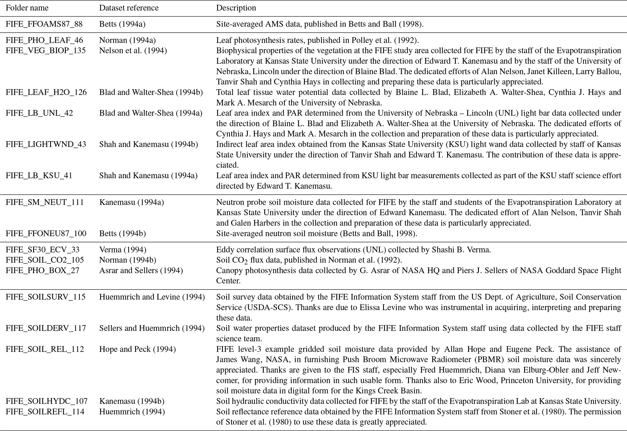
This section discusses the use of the observations and the alternative datasets considered. All of these datasets are available either in the published literature or available for download from ORNL DAAC. A list of all the ORNL DAAC datasets referred to in this paper is given in Table A1.
Betts (1994a)Betts and Ball (1998)Norman (1994a)Polley et al. (1992)Nelson et al. (1994)Blad and Walter-Shea (1994b)Blad and Walter-Shea (1994a)Shah and Kanemasu (1994b)Shah and Kanemasu (1994a)Kanemasu (1994a)Betts (1994b)(Betts and Ball, 1998)Verma (1994)Norman (1994b)Norman et al. (1992)Asrar and Sellers (1994)Huemmrich and Levine (1994)Sellers and Huemmrich (1994)Hope and Peck (1994)Kanemasu (1994b)Huemmrich (1994)Stoner et al. (1980)Table A1List of FIFE datasets from ORNL DAAC referenced in this document. Each dataset is referred to by its folder name.
A1 Driving data
This study used a 30 min resolution combined data product (FIFE_FFOAMS87_88) from observations from portable AMS data across the FIFE area, described in Betts and Ball (1998). Descriptions and references to all the FIFE datasets available from ORNL DAAC are given in Table A1. Extensive manual processing was undertaken to clean the station data before they were combined into the site-averaged data product (Betts and Ball, 1998).
The fraction of diffuse radiation is an important driving variable when the full layered canopy scheme is used in JULES (Mercado et al., 2007), although it is frequently not available and so set to a constant. For our study, we calculate diffuse radiation from shortwave radiation using the method in Weiss and Norman (1985). This method was used successfully at the FIFE site by Kim and Verma (1991a) and Kim and Verma (1991b). We also investigated using the hourly cloud observations of Marshall AAF, Kansas, approximately 12 km west of the FIFE site, which were included as part of the FIFE_FFOAMS87_88 dataset, which we converted to diffuse radiation fraction using the linear relationship given in Butt et al. (2010). This relationship was derived for two sites in the Amazon, but we confirmed that this was approximately consistent with observations of sites in the Southern Great Plains region of Oklahoma and Kansas in Still et al. (2009). However, we found that the cloud cover observations were not sufficiently consistent with the shortwave radiation used to drive the model runs. There are also total cloud cover observations from the FIFE area available in FIFE_FFOAMS87_88, but these had a period of missing data between the end of August and the middle of September. It would be interesting to compare these results to the approximation for diffuse radiation used by Gu et al. (2002) for a tallgrass prairie site in Oklahoma.
Colello et al. (1998) also carried out model runs driven by the site-averaged product (FIFE_FFOAMS87_88) and applied corrections to shortwave downward radiation, longwave downward radiation and wind speed using observations from site 4439. In our study, we do not apply local corrections to the site-averaged meteorological data. However, this may be useful to consider in the future.
A2 Leaf area index
The green leaf area index values used in this paper are destructive measurements for FIFE site 4439, read from Fig. 1 of Stewart and Verma (1992), which were taken roughly once a fortnight between 26 May and 11 October 1987. These observations are plotted in Fig. A1. They correspond closely to the green LAI observations from Verma et al. (1992) and are similar to the green LAI observations for this site given in Sellers et al. (1992) for the intensive field campaigns. The LAI values used in the Cox et al. (1998) modelling study are very similar to these datasets. Destructive LAI measurements for grass LAI, non-grass LAI and total LAI are available as part of the FIFE_VEG_BIOP_135 dataset. However, the total LAI in FIFE_VEG_BIOP_135 is substantially different from the measurements in Stewart and Verma (1992), Verma et al. (1992) and Sellers et al. (1992). This was investigated in detail at the time (Kim et al., 1989). The FIFE_VEG_BIOP_135 dataset documentation estimates that there is standard error of the mean LAI in their data of around 75 % due to the inherent variability of prairie vegetation and a variation of about 25 % can be attributed to leaf curling or folding as the leaves passed over the detector, particularly an issue for drought-stressed leaves. Foliage area index measurements (i.e. includes green leaves, dead leaves, stems) are available in FIFE_LB_UNL_42 for site 4439 in 1987 and plotted in Fig. A2. FIFE_LIGHTWND_43 and FIFE_LB_KSU_41 also have foliage area index measurements for site 4439, but these were taken in 1988 or 1989, not 1987.
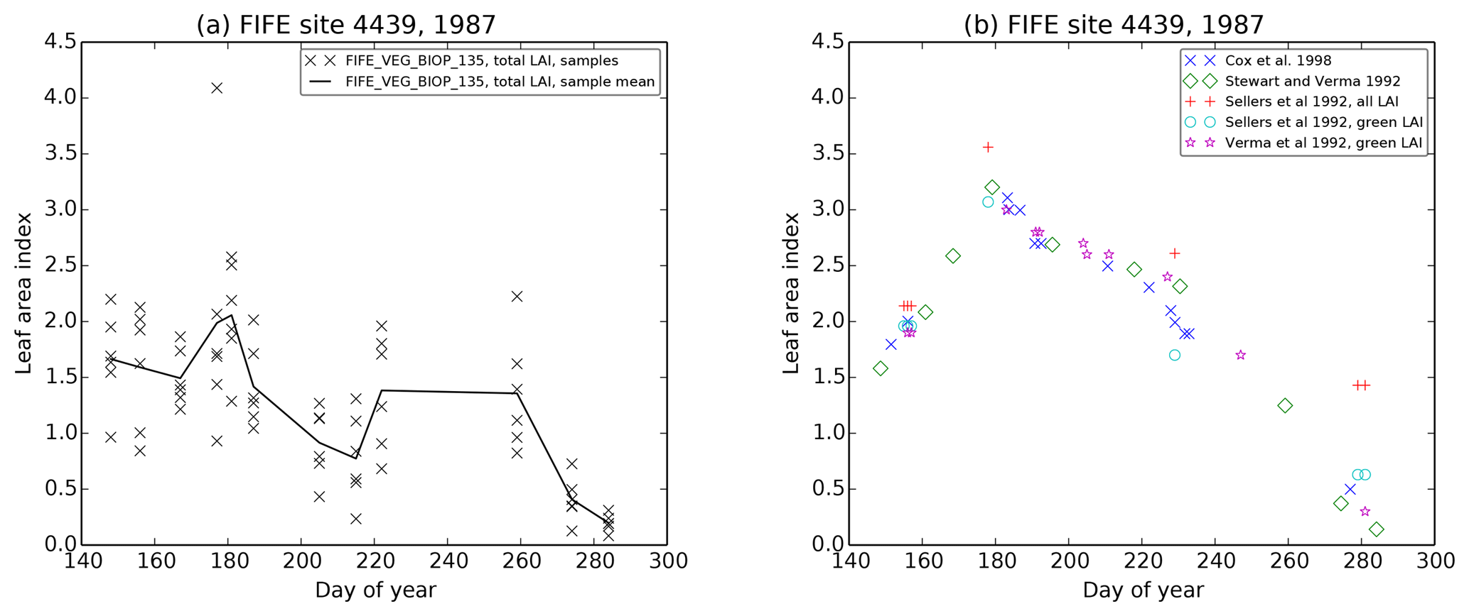
Figure A1Leaf area index observations for site 4439 for 1987. (a) Data from FIFE_VEG_BIOP_135. (b) Literature values. Plot includes data extracted from Stewart and Verma (1992) Fig. 1 and Cox et al. (1998) Fig. 1, total LAI and green LAI from Sellers et al. (1992) for the intensive field campaigns and green LAI data from Table 4 in Verma et al. (1992).
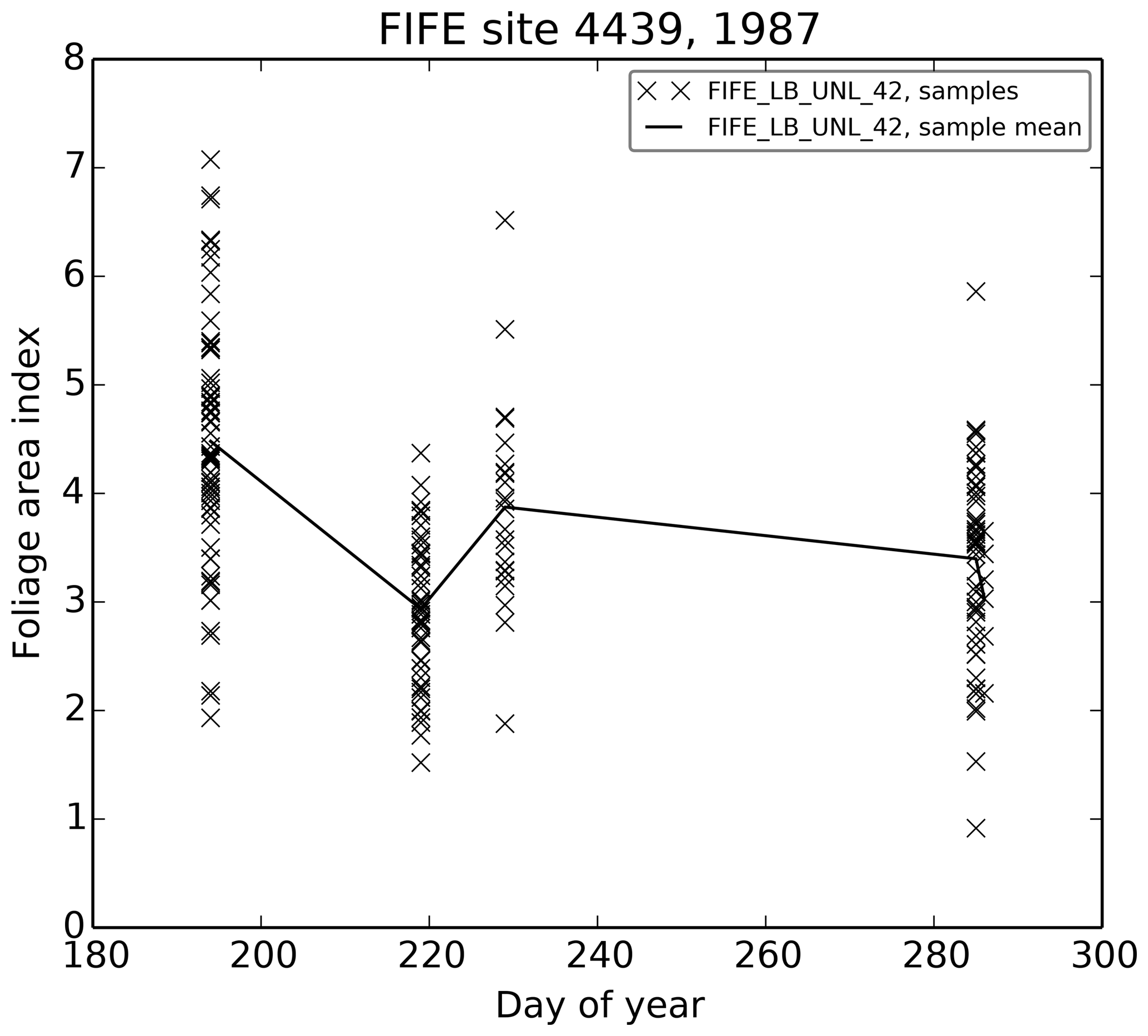
We also experimented with the internal phenology scheme in JULES. Calculating LAI dynamically with the phenology scheme would remove the need to prescribe LAI. However, we found that this scheme did not have the flexibility to reproduce the observed seasonal cycle of LAI.
A3 Soil moisture
The soil moisture data for site 4439 presented in Fig. 1 of Stewart and Verma (1992) were created from a combination gravimetric measurements and neutron probe measurements. The gravimetric measurements were taken in the top 0.1 m soil daily during the FIFE intensive field campaigns and weekly between campaigns. The neutron probe measurements were taken at different depths on 15 dates, at approximately weekly intervals between the end of May and the beginning of September 1987. These measurements were interpolated in Stewart and Verma (1992) using daily precipitation and evaporation measurements to get a daily soil moisture values for the 0–1.1 m soil layer. Stewart and Verma (1992) also observed “virtually no seasonal variation” in soil moisture below 1.1 m. The data from Stewart and Verma (1992) for the top 1.1 m of soil correspond very closely to the 0–1.6 m soil moisture values used in Cox et al. (1998) on their selected days, as illustrated in Fig. A3. Stewart and Verma (1992) also presents data for an ungrazed site in the FIFE area and states that, while the ungrazed and grazed sites received very similar season totals of precipitation, individual storms resulted in differences in soil moisture (which gives a possible motivation for using site 4439 precipitation measurements over the site-averaged data product we use here).
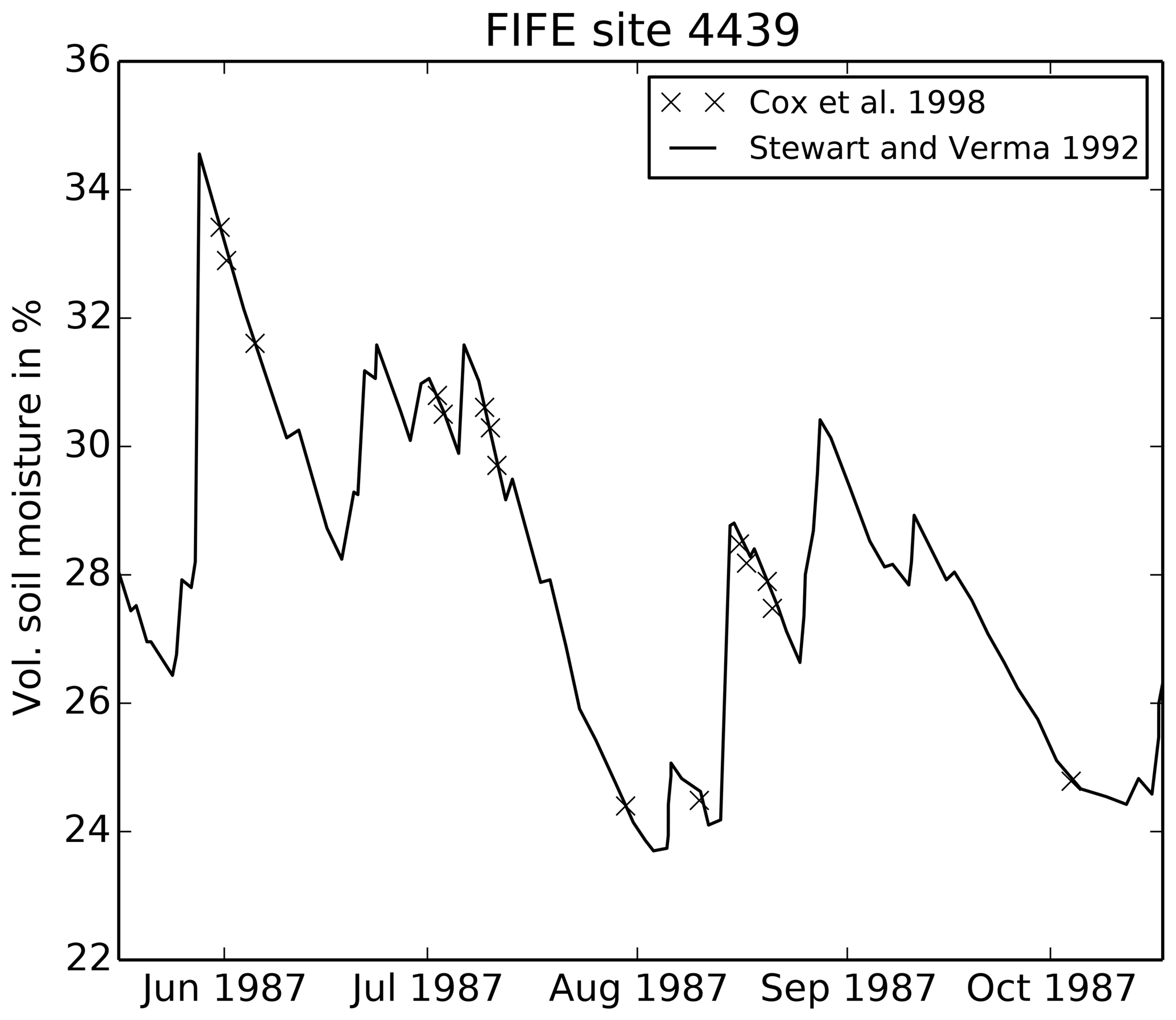
Figure A3Soil moisture data from Cox et al. (1998), compared to the derived time series of top 1.1 m soil moisture in Fig. 1 of Stewart and Verma (1992). Both datasets are for FIFE site 4439 in 1987.
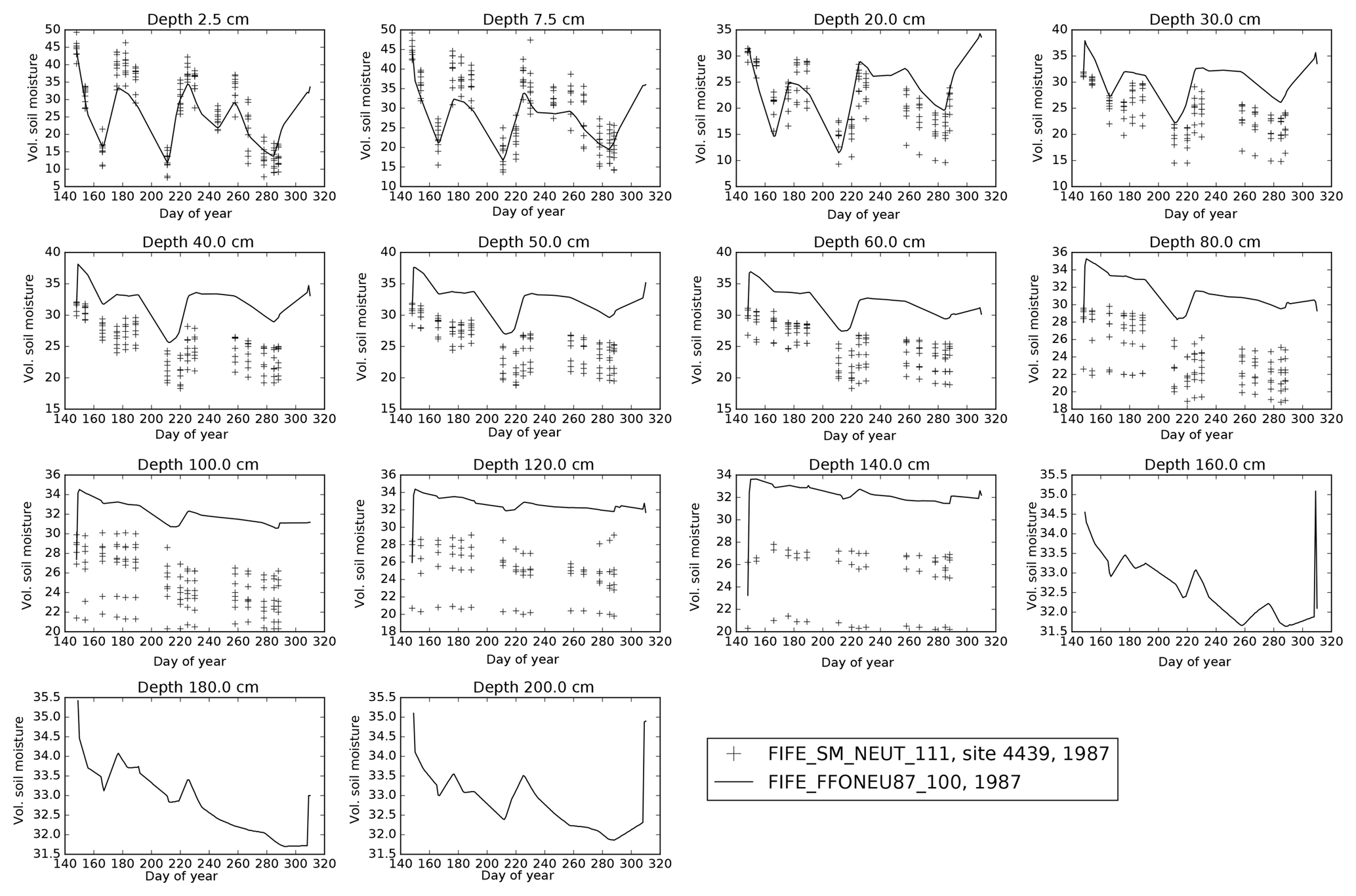
Figure A4Site-averaged soil moisture on levels from FIFE_FFONEU87_100 for 1987 (line) and individual observations of site 4439 in 1987 from FIFE_SM_NEUT_111 (points).
ORNL DAAC contains two main datasets of soil moisture observations on levels that can be considered for site 4439 for 1987: FIFE_SM_NEUT_111, which contains measurements carried out at site 4439 and FIFE_FFONEU87_100, which is a site-averaged product for the FIFE area (Betts and Ball, 1998). These are plotted in Fig. A4 for 1987. It can be seen that, at lower depths, the site 4439 measurements are considerably lower than the site-averaged product. For 1988, however, the site-averaged product is mostly within or near the edge of the spread of observations at site 4439, up to approximately 120 cm. Neither of these datasets are consistent with the Stewart and Verma (1992) site 4439 dataset when summed over the top 1.1 m. The FIFE_SM_NEUT_111 for site 8639, on the other hand, is consistent with the Stewart and Verma (1992) site 8739 dataset. The documentation for FIFE_FFONEU87_100 also cautions that the 20 cm neutron probe data is “suspect”, as the range of the probe exceeds 20 cm in dry soil and says that it is “inconsistent” with the rest of the profile in 1987. It has been linearly interpolated between observation dates. Plots of observed soil profiles for 9 and 31 July 1987 are presented in Kim and Verma (1990a). Soil profiles for individual days are also presented in Colello et al. (1998), which are consistent with the neutron probe measurements in FIFE_SM_NEUT_111 but not the gravimetric measurements. Given these inconsistencies, we chose not to use the soil moisture observations for individual levels to directly drive our simulations.
Derived soil moisture
In order to create a daily soil moisture time series on levels, which could
be used to drive the global-C4-grass and tune-leaf runs, we
used a Python implementation of the JULES hydrology scheme. The soil layer
thicknesses used were the same as in Harper et al. (2016), apart from
the third soil layer, which was extended by 10 cm. This meant that the total
depth of the top three layers was 1.1 m, which meant that we could constrain
the sum of the soil moisture in the top three levels in our runs to be equal
to the daily 0–1.1 m soil moisture values from Stewart and Verma (1992).
We assumed that positive changes in the 0–1.1 m soil moisture were due to
rainfall (with runoff, canopy evaporation and soil evaporation from that day
already subtracted) and therefore added it to the top layer, while negative
changes in the 0–1.1 m soil moisture were assumed to be due to transpiration
(corrected for the transpiration flux from the lowest level and the flux
between the lowest and second-to-lowest layer), which was taken from the soil
layers according to an exponential root distribution with e-fold depth
dr=0.5 m. This dr depth is the same as natural C4 grass in
Harper et al. (2016). We used the same soil hydrological parameters as
in our JULES simulations (described in Sect. A4).

Figure A5(a) Derived soil moisture dataset, on model soil levels. (b) Derived soil moisture in the top layer, compared to the gravimetric soil moisture measurements for 2.5 and 7.5 cm from FIFE_SM_NEUT_111.
Table A2JULES parameters used to represent vegetation at FIFE site 4439,
which vary across runs. These parameters are all specified in the
JULES_PFTPARM namelist apart from can_rad_mod
(JULES_VEGETATION), co2_mmr (JULES_CO2) and
beta2 (JULES_SURFACE).
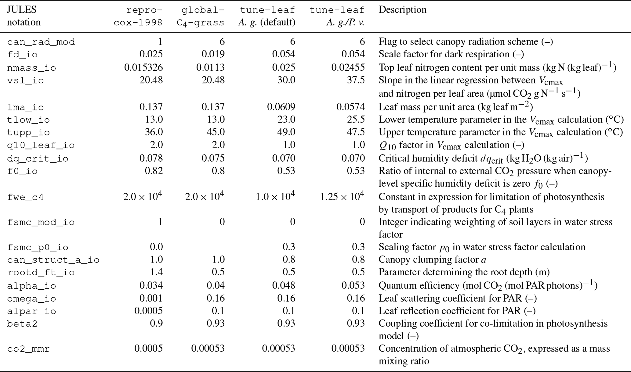
The resulting derived soil moisture time series are shown in Fig. A5 (left). As expected, the upper levels show more variability than the lower levels, which is consistent with the site grid 4439 and site-averaged soil moisture time series on levels (see Sect. A3) and approximately with the statement in Stewart and Verma (1992) that there was “virtually no seasonal variation” below 1.1 m. Figure A5b compares the derived time series for soil moisture in the top soil level (10 cm thickness) to the gravimetric soil moisture data for 2.5 and 7.5 cm from FIFE_SM_NEUT_111. While the fit is reasonable, given the spread in observations, it appears to indicate that the variability in the top level soil moisture is still underestimated. This could be due to the assumed root distribution (a lower dr would lead to more water extracted from the upper layer) or the approximation that soil evaporation can be neglected on days without rainfall, or approximations made by Stewart and Verma (1992) when deriving the 1.1 m soil moisture time series.
Table A3Parameter combinations used for the f0, dqcrit sensitivity studies.
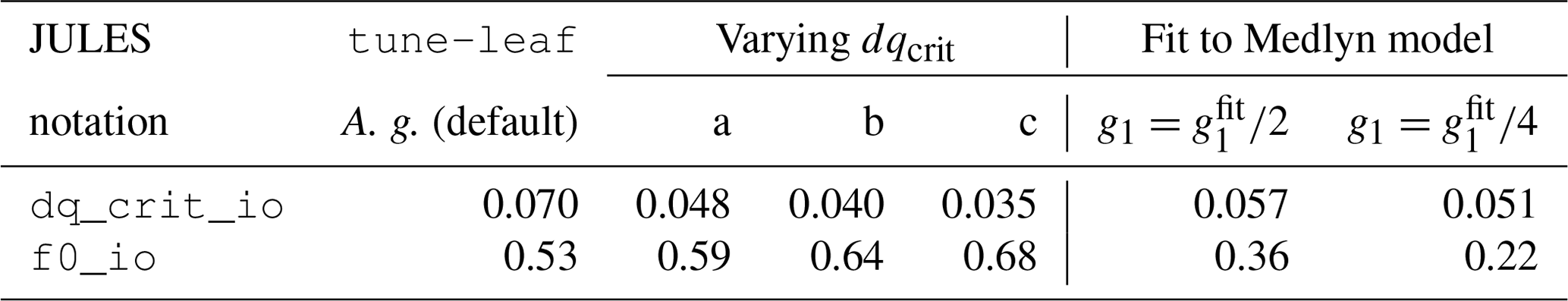
We also attempted two other methods for deriving a soil moisture time series
on levels from Stewart and Verma (1992) using the transpiration from
the repro-cox-1998 run and editing the repro-cox-1998 run
so that soil moisture was no longer prescribed. The first method did not
perform well, possibly due to the transpiration and soil moisture time series
not quite being in step with each other. The second method worked well if the
canopy capacity at zero LAI was reduced (in JULES, the canopy capacity is a
linear function of LAI) and the PFT infiltration enhancement factor
increased. Interestingly, Colello et al. (1998) concluded that they
needed to change the infiltration and canopy interception capacity for this
site. There was an issue capturing one of the peaks in the surface soil
moisture in the spring, which was probably due to missing data in the
rainfall dataset: the local-day maximum in FIFE_FFOAMS87_88 from
day 130 to day 150 was 42.71 mm, which occurred on day 147, which had nine
missing time steps. In contrast, the local-day maximum from for this interval
in Stewart and Verma (1992) was much higher, at around 70 mm.
A4 Soil properties
This section discusses and compares the available measurements of the hydraulic, thermal and optical soil properties, which can be used as ancillary data for runs at FIFE site 4439. Soil in the FIFE area was extensively studied. At site 4439, the soil was classified as predominantly Dwight silty clay loam (Typic Natrustolls) (Verma et al., 1992). Colello et al. (1998) describes the soil column as being “about 140 cm in depth, changing from silty-clay-loam to clay to gravel to impermeable bedrock”.
In our simulations, each soil ancillary variable was set to be constant throughout the soil column. The two most important soil parameters are the “wilting” soil moisture θwilt and “critical” soil moisture θcrit, which we define as the volumetric soil moisture at −0.033 and −1.5 MPa, respectively (following Cox et al., 1998 and Best et al., 2011). These soil parameters enter directly into the soil moisture stress calculation. In all of our simulations, θwilt was set to 0.205 and θcrit was set to 0.387, taken from Cox et al. (1998) (which quotes Stewart and Verma, 1992, although these values do not appear in this paper explicitly). In contrast, Verma et al. (1989) state that the surface (0 to 0.05 m) wilting and critical soil moisture values were approximately 15.0 % and 39.4 %, respectively. It is also possible to obtain the wilting and critical soil moisture values used in Verma et al. (1992) from comparing their extractable water values to volumetric soil moisture measurements from individual days in Cox et al. (1998). This leads to wilting and critical soil moisture values of 20.1 % and 34.8 %, respectively.
We used the Brooks and Corey (1964) relation between soil water content θ and absolute matric potential Ψ:
where S denotes values at saturation to obtain the Brooks–Corey parameter b and the soil water suction at saturation ΨS from the Cox et al. (1998) values of θwilt and θcrit. The other hydraulic and thermal soil ancillary variables were calculated from the fraction of sand, silt and clay given for Dwight soil in FIFE_SOILSURV_115, averaged over 0–122 cm, using the relations from Cosby et al. (1984). The soil albedo (0.162) was calculated from the Munsell colour value for dry Dwight soil given in FIFE_SOILSURV_115, averaged over 0–122 cm, using the relation in Post et al. (2000). This was consistent with the reflectance data for Dwight soil in FIFE_SOILREFL_114 (which had a mean of 0.153, a standard deviation of 0.055 and was taken at a range of wavelengths).
There are also measurements available at specified depths. FIFE_SOILSURV_115 contains observations for clay, silt, sand and organic carbon content, bulk density, wilting and critical soil moisture values for Dwight soil at different depths (these data are from site 2731, but it states that these data can also be used for site 4439, because the two sites have similar soil series). The relations in Cosby et al. (1984) can be used to convert the clay, sand and silt fractions to the soil hydraulic and thermal parameters needed by JULES. These can be corrected for organic content using Dankers et al. (2011) and Chadburn et al. (2015). The FIFE_SOIL_REL_112 dataset contains site 4439 bulk density and soil water potentials at different volumetric soil content (including the wilting and critical soil moisture values). FIFE_SOILDERV_117 has soil porosity, saturated water potential and the b parameter from Eq. (A1) for site 4439. Water retention curves plotted using these data are consistent with the data in FIFE_SOIL_REL_112 (not shown). Hydraulic conductivity for site 4439 is provided in FIFE_SOILHYDC_107. Bulk density can be converted to saturation volumetric soil moisture using the relation given in the FIFE_SOILDERV_117 documentation.
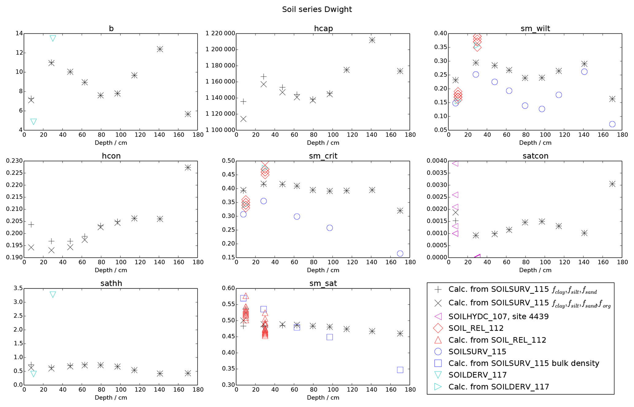
Figure A6Soil ancillary variables needed by JULES, using the notation from
the JULES namelists. When JULES is set to use soil hydraulic characteristics
from Brooks and Corey (1964), these are b (exponent in soil
hydraulic characteristics, i.e. b in Eq. A1), hcap
(dry heat capacity in J m−3 K−1), sm_wilt (volumetric
soil moisture content at −1.5 MPa, θwilt), hcon
(dry thermal conductivity in W m−1 K−1), sm_crit
(volumetric soil moisture content at MPa, θcrit),
satcon (hydraulic conductivity at saturation in
kg m−2 s−1), sathh (absolute value of the soil matric
suction at saturation ΨS in m) and sm_sat
(volumetric soil moisture content at saturation
θS).
The resulting soil hydraulic and thermal parameters from these different methods are plotted in Fig. A6 and show that there are considerable differences between the different datasets. The large spread in the wilting and critical soil moisture values is particularly important to note, since, as we have discussed, they both enter the soil moisture stress factor β explicitly, and therefore plant GPP and transpiration are very sensitive to variations in these parameters. The thermal and optical soil properties and the remaining hydraulic properties have a comparatively minor effect on GPP and evapotranspiration.
A5 Canopy height
In this study, we used the canopy height observations presented in Table 2 of Verma et al. (1992): 0.4–0.6, 0.6–0.75 and 0.75–0.9 m for days 120–179, 180–239 and 240–300, respectively, for site 16 in 1987. Another available dataset for canopy height at this site is FIFE_VEG_BIOP_135, which is plotted in Fig. A7, and shows considerable differences with the Verma et al. (1992) data, particularly in the 240- to 300-day period. As discussed in Sect. A2, the non-uniformity of the vegetation at this site is a significant source of error in these measurements.

A6 Canopy dark respiration
Polley et al. (1992) shows leaf dark respiration as a function of leaf temperature for observations of A. gerardii, S. nutans and P. virgatum taken in the FIFE area in 1987 and fits the following relationship:
When this relation was used in Cox et al. (1998), it was scaled up to the canopy level by multiplying by LAI, i.e. dark respiration was assumed to be constant on leaves through the canopy. In contrast, in the model presented in Kim and Verma (1991a), leaf respiration was calculated from
where µmol m−2 s−1, R=8.314 J K−1 mol−1 is the gas constant and Tl is the leaf temperature in ∘C and leaf dark respiration was suppressed by 50 % when the absorbed PAR was greater than 20 µmol quanta m−2 s−1, to account for the light dependency of mitochondrial respiration. Air temperature near the top of the canopy was used to approximate leaf temperature. Kim and Verma (1991a) scaled this leaf respiration up to the canopy level by considering the sunlit and shaded portions of the leaf separately.
In JULES, dark respiration decreases through the canopy in the same way as
Vcmax and it is multiplied by the soil moisture stress parameter
β. In the “big leaf” approximation used in the repro-cox-1998
run, Vcmax decreases through the canopy with light. In the layered
canopy model with sunflecks used in the global-C4-grass and
tune-leaf runs, the decrease of Vcmax through the canopy is set
by an input parameter knl, and the leaf dark respiration is reduced by a
factor of 30 % above a light threshold.
A7 Net canopy assimilation
In this study, we compared the net canopy carbon assimilation from the model (for GPP minus respiration from leaves) to two different datasets. The first dataset was read from Figs. 1–4 in Kim and Verma (1991a), for 5 June, 2 July, 30 July and 20 August 1987, which was obtained from eddy correlations of atmospheric CO2, measured above the canopy. Leaf respiration was calculated from Eq. (A3), as described in Sect. A6. The leaf respiration over the entire canopy was subtracted from the nighttime CO2 flux from the night following or proceeding the day under consideration, to calculate the other sources of respiration (soil, root), which were adjusted to daytime soil temperatures using a Q10 factor of 2.
The second net canopy carbon assimilation dataset was created from FIFE_SF30_ECV_33 observations of CO2 flux from eddy correlation techniques using the procedure in Cox et al. (1998). The total respiration Fs in Cox et al. (1998) was fitted to the functional form proposed by Norman et al. (1992) for use when LAI measurements were not available, evaluated with FIFE data:
where Ts,10 is the 10 cm soil temperature in ∘C, and s1, s2 and s3 are fitted parameters. Using air temperature in the place of the soil temperature, Cox et al. (1998) found that using this expression with the parameter values s1=17.8 µmol CO2 m−2 s−1, s2=0.2, s3=0.062 ∘C−1 explained 50.7 % of the variance in nighttime CO2 flux measurements at FIFE. Leaf-level dark respiration was calculated using Eq. (A2), scaling from leaf level to canopy level by multiplying by LAI, as described in Sect. A6, assuming that the leaf temperature and the air temperature were the same (we used the air temperatures in FIFE_SF30_ECV_33).
Canopy measurements taken in a Plexiglas chamber (FIFE_PHO_BOX_27) at four sites, including 4439, could possibly be used as an additional source of net canopy assimilation for comparison with the model. It would also be interesting to extend the analysis to include an evaluation of the modelled soil respiration. The model could be compared directly to the fitted expressions for soil respiration (with and without a LAI dependence) from Norman et al. (1992) or, alternatively, to the soil CO2 flux measurements available in FIFE_SOIL_CO2_105.
The supplement related to this article is available online at: https://doi.org/10.5194/gmd-12-3207-2019-supplement.
KEW designed and performed the analysis with advice from co-authors; ABH, CH, LMM, CTM, PDF, PMC and JK read and commented on the manuscript.
The authors declare that they have no conflict of interest.
We wish to express our respect and gratitude to the FIFE investigators. FIFE was a monumental scientific achievement and its legacy will be long-lasting. We would like to thank Tim Arkebauer for information about the FIFE leaf gas exchange observations from Polley et al. (1992).
Karina E. Williams and Pete D. Falloon received financial support from the European Commission (grant IMPREX 641811), Karina E. Williams, Camilla T. Mathison and Pete D. Falloon from the Met Office Hadley Centre Climate Programme funded by BEIS and Defra, Chris Huntingford from the NERC/CEH National Capability Fund and Lina M. Mercado from the UK Natural Environment Research Council through the UK Earth System Modelling Project (UKESM, grant no. NE/N017951/1).
This paper was edited by Jatin Kala and reviewed by three anonymous referees.
Asrar, G. and Sellers, P. J.: Canopy Photosynthesis Rates (FIFE), data set, Oak Ridge National Laboratory Distributed Active Archive Center, Oak Ridge, Tennessee, USA, https://doi.org/10.3334/ORNLDAAC/27, also published in: Strebel, D. E., Landis, D. R., Huemmrich, K. F., and Meeson, B. W. (Eds.): Collected Data of the First ISLSCP Field Experiment, Vol. 1: Surface Observations and Non-Image Data Sets. CD-ROM. National Aeronautics and Space Administration, Goddard Space Flight Center, Greenbelt, Maryland, USA, available at: http://daac.ornl.gov (last access: 30 May 2019), 1994. a
Baldocchi, D., Falge, E., Gu, L., Olson, R., Hollinger, D., Running, S., Anthoni, P., Bernhofer, C., Davis, K., Evans, R., Fuentes, J., Goldstein, A., Katul, G., Law, B., Lee, X., Malhi, Y., Meyers, T., Munger, W., Oechel, W., Paw, K. T., Pilegaard, K., Schmid, H. P., Valentini, R., Verma, S., Vesala, T., Wilson, K., and Wofsy, S.: FLUXNET: A New Tool to Study the Temporal and Spatial Variability of Ecosystem–Scale Carbon Dioxide, Water Vapor, and Energy Flux Densities, B. Am. Meteorol. Soc., 82, 2415–2434, https://doi.org/10.1175/1520-0477(2001)082<2415:fantts>2.3.co;2, 2001. a
Best, M. J., Pryor, M., Clark, D. B., Rooney, G. G., Essery, R. L. H., Ménard, C. B., Edwards, J. M., Hendry, M. A., Porson, A., Gedney, N., Mercado, L. M., Sitch, S., Blyth, E., Boucher, O., Cox, P. M., Grimmond, C. S. B., and Harding, R. J.: The Joint UK Land Environment Simulator (JULES), model description – Part 1: Energy and water fluxes, Geosci. Model Dev., 4, 677–699, https://doi.org/10.5194/gmd-4-677-2011, 2011. a, b, c, d
Betts, A. K.: Site Averaged AMS Data: 1987 (Betts), data set, Oak Ridge National Laboratory Distributed Active Archive Center, Oak Ridge, Tennessee, USA, https://doi.org/10.3334/ORNLDAAC/88, 1994a. a
Betts, A. K.: Site Averaged Neutron Soil Moisture: 1987 (Betts), data set, Oak Ridge National Laboratory Distribute d Active Archive Center, Oak Ridge, Tennessee, USA, https://doi.org/10.3334/ORNLDAAC/100, 1994b. a
Betts, A. K. and Ball, J. H.: FIFE Surface Climate and Site-Average Dataset 1987–89, J. Atmos. Sci., 55, 1091–1108, https://doi.org/10.1175/1520-0469(1998)055<1091:fscasa>2.0.co;2, 1998. a, b, c, d, e, f, g, h, i, j, k, l, m
Blad, B. L. and Walter-Shea, E. A.: LAI and PAR Data: Light Bar – UNL (FIFE), data set, Oak Ridge National Laboratory Distributed Active Archive Center, Oak Ridge, Tennessee, USA, https://doi.org/10.3334/ORNLDAAC/42, also published in: Strebel, D. E., Landis, D. R., Huemmrich, K. F., and Meeson, B. W. (Eds.): Collected Data of the First ISLSCP Field Experiment, Vol. 1: Surface Observations and Non-Image Data Sets. CD-ROM. National Aeronautics and Space Administration, Goddard Space Flight Center, Greenbelt, Maryland, USA, available at: http://daac.ornl.gov (last access: 30 May 2019), 1994a. a
Blad, B. L. and Walter-Shea, E. A.: Total Leaf Tissue Water Potential (FIFE), data set, Oak Ridge National Laboratory Distributed Active Archive Center, Oak Ridge, Tennessee, USA, https://doi.org/10.3334/ORNLDAAC/126, also published in: Strebel, D. E., Landis, D. R., Huemmrich, K. F., and Meeson, B. W. (Eds.): Collected Data of the First ISLSCP Field Experiment, Vol. 1: Surface Observations and Non-Image Data Sets. CD-ROM. National Aeronautics and Space Administration, Goddard Space Flight Center, Greenbelt, Maryland, USA, available at http://daac.ornl.gov (last access: 30 May 2019), 1994b. a
Blair, J., Nippert, J., and Briggs, J.: Grassland Ecology, chap. 14, 389–423, Springer New York, New York, NY, https://doi.org/10.1007/978-1-4614-7501-9_14, 2014a. a, b
Blair, J. M., Baer, S. G., Dodds, W. K., Joern, A., and Nippert, J. B.: LTER Project Proposal: Long-Term Research on Grassland Dynamics- Assessing Mechanismsof Sensitivity and Resilience to Global Change, available at: http://lter.konza.ksu.edu/sites/default/files/LTERVIIonline.pdf (last access: 30 May 2019), 2014b. a
Brooks, R. H. and Corey, A. T.: Hydraulic properties of porous media, Tech. Rep. 3, Colorado State University, Fort Collins, Colorado, USA, 1964. a, b
Butt, N., New, M., Malhi, Y., da Costa, A. C., Oliveira, P., and Silva-Espejo, J. E.: Diffuse radiation and cloud fraction relationships in two contrasting Amazonian rainforest sites, Agr. Forest Meteorol., 150, 361–368, https://doi.org/10.1016/j.agrformet.2009.12.004, 2010. a
Chadburn, S., Burke, E., Essery, R., Boike, J., Langer, M., Heikenfeld, M., Cox, P., and Friedlingstein, P.: An improved representation of physical permafrost dynamics in the JULES land-surface model, Geosci. Model Dev., 8, 1493–1508, https://doi.org/10.5194/gmd-8-1493-2015, 2015. a
Clark, D. B., Mercado, L. M., Sitch, S., Jones, C. D., Gedney, N., Best, M. J., Pryor, M., Rooney, G. G., Essery, R. L. H., Blyth, E., Boucher, O., Harding, R. J., Huntingford, C., and Cox, P. M.: The Joint UK Land Environment Simulator (JULES), model description – Part 2: Carbon fluxes and vegetation dynamics, Geosci. Model Dev., 4, 701–722, https://doi.org/10.5194/gmd-4-701-2011, 2011. a, b
Colello, G. D., Grivet, C., Sellers, P. J., and Berry, J. A.: Modeling of Energy, Water, and CO2 Flux in a Temperate Grassland Ecosystem with SiB2: May–October 1987, J. Atmos. Sci., 55, 1141–1169, https://doi.org/10.1175/1520-0469(1998)055<1141:moewac>2.0.co;2, 1998. a, b, c, d, e, f
Collatz, G. J., Ribas-Carbo, M., and Berry, J. A.: Coupled Photosynthesis-Stomatal Conductance Model for Leaves of C4 Plants, Aust. J. Plant Physiol., 19, 519–538, 1992. a, b
Cosby, B. J., Hornberger, G. M., Clapp, R. B., and Ginn, T. R.: A Statistical Exploration of the Relationships of Soil Moisture Characteristics to the Physical Properties of Soils, Water Resour. Res., 20, 682–690, https://doi.org/10.1029/wr020i006p00682, 1984. a, b
Cox, P. M., Huntingford, C., and Harding, R. J.: A canopy conductance and photosynthesis model for use in a GCM land surface scheme, J. Hydrol., 212–213, 79–94, https://doi.org/10.1016/s0022-1694(98)00203-0, 1998. a, b, c, d, e, f, g, h, i, j, k, l, m, n, o, p, q, r, s, t, u, v, w, x, y, z, aa, ab, ac, ad, ae, af, ag, ah, ai, aj, ak, al, am, an, ao, ap
Dai, Y., Dickinson, R. E., and Wang, Y.-P.: A Two-Big-Leaf Model for Canopy Temperature, Photosynthesis, and Stomatal Conductance, J. Climate, 17, 2281–2299, https://doi.org/10.1175/1520-0442(2004)017<2281:atmfct>2.0.co;2, 2004. a
Dankers, R., Burke, E. J., and Price, J.: Simulation of permafrost and seasonal thaw depth in the JULES land surface scheme, The Cryosphere, 5, 773–790, https://doi.org/10.5194/tc-5-773-2011, 2011. a
De Kauwe, M. G., Kala, J., Lin, Y.-S., Pitman, A. J., Medlyn, B. E., Duursma, R. A., Abramowitz, G., Wang, Y.-P., and Miralles, D. G.: A test of an optimal stomatal conductance scheme within the CABLE land surface model, Geosci. Model Dev., 8, 431–452, https://doi.org/10.5194/gmd-8-431-2015, 2015. a, b
Dewar, R. C.: The Ball–Berry–Leuning and Tardieu–Davies stomatal models: synthesis and extension within a spatially aggregated picture of guard cell function, Plant Cell Environ., 25, 1383–1398, https://doi.org/10.1046/j.1365-3040.2002.00909.x, 2002. a
Eller, C. B., Rowland, L., Oliveira, R. S., Bittencourt, P. R. L., Barros, F. V., da Costa, A. C. L., Meir, P., Friend, A. D., Mencuccini, M., Sitch, S., and Cox, P.: Modelling tropical forest responses to drought and El Niño with a stomatal optimization model based on xylem hydraulics, Philos. T. Roy. Soc. B, 373, 20170315, https://doi.org/10.1098/rstb.2017.0315, 2018. a
Fierer, N., Ladau, J., Clemente, J. C., Leff, J. W., Owens, S. M., Pollard, K. S., Knight, R., Gilbert, J. A., and McCulley, R. L.: Reconstructing the Microbial Diversity and Function of Pre-Agricultural Tallgrass Prairie Soils in the United States, Science, 342, 621–624, https://doi.org/10.1126/science.1243768, 2013. a
Gu, L., Baldocchi, D., Verma, S. B., Black, T. A., Vesala, T., Falge, E. M., and Dowty, P. R.: Advantages of diffuse radiation for terrestrial ecosystem productivity, J. Geophys. Res., 107, 2–ACL 2–23, https://doi.org/10.1029/2001jd001242, 2002. a
Harper, A. B., Cox, P. M., Friedlingstein, P., Wiltshire, A. J., Jones, C. D., Sitch, S., Mercado, L. M., Groenendijk, M., Robertson, E., Kattge, J., Bönisch, G., Atkin, O. K., Bahn, M., Cornelissen, J., Niinemets, Ü., Onipchenko, V., Peñuelas, J., Poorter, L., Reich, P. B., Soudzilovskaia, N. A., and Bodegom, P. V.: Improved representation of plant functional types and physiology in the Joint UK Land Environment Simulator (JULES v4.2) using plant trait information, Geosci. Model Dev., 9, 2415–2440, https://doi.org/10.5194/gmd-9-2415-2016, 2016. a, b, c, d, e, f, g, h, i, j, k
Harper, A. B., Wiltshire, A. J., Cox, P. M., Friedlingstein, P., Jones, C. D., Mercado, L. M., Sitch, S., Williams, K., and Duran-Rojas, C.: Vegetation distribution and terrestrial carbon cycle in a carbon cycle configuration of JULES4.6 with new plant functional types, Geosci. Model Dev., 11, 2857–2873, https://doi.org/10.5194/gmd-11-2857-2018, 2018. a
Hope, A. and Peck, E. L.: Soil Moisture Release Data (FIFE), data set, Oak Ridge National Laboratory Distributed Active Archive Center, Oak Ridge, Tennessee, USA, https://doi.org/10.3334/ORNLDAAC/112, also published in: Strebel, D. E., Landis, D. R., Huemmrich, K. F., and Meeson, B. W. (Eds.): Collected Data of the First ISLSCP Field Experiment, Vol. 1: Surface Observations and Non-Image Data Sets. CD-ROM. National Aeronautics and Space Administration, Goddard Space Flight Center, Greenbelt, Maryland, USA, available at: http://daac.ornl.gov (last access: 30 May 2019), 1994. a
Huemmrich, K. F.: Soil Reflectance Data (FIFE), data set, Oak Ridge National Laboratory Distributed Active Archive Center, Oak Ridge, Tennessee, USA, https://doi.org/10.3334/ORNLDAAC/114, also published in: Strebel, D. E., Landis, D. R., Huemmrich, K. F., and Meeson, B. W. (Eds.): Collected Data of the First ISLSCP Field Experiment, Vol. 1: Surface Observations and Non-Image Data Sets. CD-ROM. National Aeronautics and Space Administration, Goddard Space Flight Center, Greenbelt, Maryland, USA, available at: http://daac.ornl.gov (last access: 30 May 2019), 1994. a
Huemmrich, K. F. and Levine, E.: Soil Survey Reference (FIFE), data set, Oak Ridge National Laboratory Distributed Active Archive Center, Oak Ridge, Tennessee, USA, https://doi.org/10.3334/ORNLDAAC/115, also published in: Strebel, D. E., Landis, D. R., Huemmrich, K. F., and Meeson, B. W. (Eds.): Collected Data of the First ISLSCP Field Experiment, Vol. 1: Surface Observations and Non-Image Data Sets. CD-ROM. National Aeronautics and Space Administration, Goddard Space Flight Center, Greenbelt, Maryland, USA, available at: http://daac.ornl.gov (last access: 30 May 2019), 1994. a
Huntingford, C., Smith, D. M., Davies, W. J., Falk, R., Sitch, S., and Mercado, L. M.: Combining the [ABA] and net photosynthesis-based model equations of stomatal conductance, Ecol. Model., 300, 81–88, https://doi.org/10.1016/j.ecolmodel.2015.01.005, 2015. a
Jacobs, C. M. J.: Direct impact of atmospheric CO2 enrichment on regional transpiration, PhD thesis, Wageningen Agricultural University, Wageningen, the Netherlands, 1994. a, b, c
Kanemasu, E. T.: Soil Moisture Neutron Probe Data (FIFE), data set, Oak Ridge National Laboratory Distributed Active Archive Center, Oak Ridge, Tennessee, USA, https://doi.org/10.3334/ORNLDAAC/111, also published in: Strebel, D. E., Landis, D. R., Huemmrich, K. F., and Meeson, B. W. (Eds.): Collected Data of the First ISLSCP Field Experiment, Vol. 1: Surface Observations and Non-Image Data Sets. CD-ROM. National Aeronautics and Space Administration, Goddard Space Flight Center, Greenbelt, Maryland, USA, available at: http://daac.ornl.gov (last access: 30 May 2019), 1994a. a
Kanemasu, E. T.: Soil Hydraulic Conductivity Data (FIFE), data set, Oak Ridge National Laboratory Distributed Active Archive Center, Oak Ridge, Tennessee, USA, https://doi.org/10.3334/ORNLDAAC/107, also published in: Strebel, D. E., Landis, D. R., Huemmrich, K. F., and Meeson, B. W. (Eds.): Collected Data of the First ISLSCP Field Experiment, Vol. 1: Surface Observations and Non-Image Data Sets. CD-ROM. National Aeronautics and Space Administration, Goddard Space Flight Center, Greenbelt, Maryland, USA, available at: http://daac.ornl.gov (last access: 30 May 2019), 1994b. a
Kattge, J., Díaz, S., Lavorel, S., Prentice, I. C., Leadley, P., Bönisch, G., Garnier, E., Westoby, M., Reich, P. B., Wright, I. J., Cornelissen, J. H. C., Violle, C., Harrison, S. P., Van BODEGOM, P. M., Reichstein, M., Enquist, B. J., Soudzilovskaia, N. A., Ackerly, D. D., Anand, M., Atkin, O., Bahn, M., Baker, T. R., Baldocchi, D., Bekker, R., Blanco, C. C., Blonder, B., Bond, W. J., Bradstock, R., Bunker, D. E., Casanoves, F., Cavender-Bares, J., Chambers, J. Q., Chapin, F. S., Chave, J., Coomes, D., Cornwell, W. K., Craine, J. M., Dobrin, B. H., Duarte, L., Durka, W., Elser, J., Esser, G., Estiarte, M., Fagan, W. F., Fang, J., Fernández-Méndez, F., Fidelis, A., Finegan, B., Flores, O., Ford, H., Frank, D., Freschet, G. T., Fyllas, N. M., Gallagher, R. V., Green, W. A., Gutierrez, A. G., Hickler, T., Higgins, S. I., Hodgson, J. G., Jalili, A., Jansen, S., Joly, C. A., Kerkhoff, A. J., Kirkup, D., Kitajima, K., Kleyer, M., Klotz, S., Knops, J. M. H., Kramer, K., Kühn, I., Kurokawa, H., Laughlin, D., Lee, T. D., Leishman, M., Lens, F., Lenz, T., Lewis, S. L., Lloyd, J., Llusià, J., Louault, F., Ma, S., Mahecha, M. D., Manning, P., Massad, T., Medlyn, B. E., Messier, J., Moles, A. T., Müller, S. C., Nadrowski, K., Naeem, S., Niinemets, U., Nöllert, S., Nüske, A., Ogaya, R., Oleksyn, J., Onipchenko, V. G., Onoda, Y., Ordoñez, J., Overbeck, G., Ozinga, W. A., Patiño, S., Paula, S., Pausas, J. G., Peñuelas, J., Phillips, O. L., Pillar, V., Poorter, H., Poorter, L., Poschlod, P., Prinzing, A., Proulx, R., Rammig, A., Reinsch, S., Reu, B., Sack, L., Salgado-Negret, B., Sardans, J., Shiodera, S., Shipley, B., Siefert, A., Sosinski, E., Soussana, Swaine, E., Swenson, N., Thompson, K., Thornton, P., Waldram, M., Weiher, E., White, M., White, S., Wright, S. J., Yguel, B., Zaehle, S., Zanne, A. E., and Wirth, C.: TRY – a global database of plant traits, Glob. Change Biol., 17, 2905–2935, https://doi.org/10.1111/j.1365-2486.2011.02451.x, 2011. a, b
Kim, J. and Verma, S.: Components of surface energy balance in a temperate grassland ecosystem, Bound.-Lay. Meteorol., 51, 401–417, https://doi.org/10.1007/bf00119676, 1990a. a, b, c, d, e, f, g
Kim, J. and Verma, S. B.: Carbon dioxide exchange in a temperate grassland ecosystem, Bound.-Lay. Meteorol., 52, 135–149, https://doi.org/10.1007/bf00123181, 1990b. a
Kim, J. and Verma, S. B.: Modeling canopy photosynthesis: scaling up from a leaf to canopy in a temperate grassland ecosystem, Agr. Forest Meteorol., 57, 187–208, https://doi.org/10.1016/0168-1923(91)90086-6, 1991a. a, b, c, d, e, f, g, h, i, j, k, l, m, n, o, p, q
Kim, J. and Verma, S. B.: Modeling canopy stomatal conductance in a temperate grassland ecosystem, Agr. Forest Meteorol., 55, 149–166, https://doi.org/10.1016/0168-1923(91)90028-o, 1991b. a, b, c, d, e, f, g, h, i, j
Kim, J., Hays, C., Verma, S., and Blad, B.: A preliminary report on LAI values obtained during FIFE by various methods, Tech. rep., Center for Agricultural Meteorology and Climatology, University of Nebraska, Lincoln, USA, 1989. a
Kim, J., Verma, S. B., and Clement, R. J.: Carbon dioxide budget in a temperate grassland ecosystem, J. Geophys. Res., 97, 6057–6063, https://doi.org/10.1029/92jd00186, 1992. a
Knapp, A. K.: Effect of Fire and Drought on the Ecophysiology of Andropogon gerardii and Panicum virgatum in a Tallgrass Prairie, Ecology, 66, 1309–1320, https://doi.org/10.2307/1939184, 1985. a, b, c, d, e, f, g, h, i, j, k, l, m, n, o, p, q, r, s, t, u, v
Leuning, R.: A critical appraisal of a combined stomatal-photosynthesis model for C3 plants, Plant Cell Environ., 18, 339–355, https://doi.org/10.1111/j.1365-3040.1995.tb00370.x, 1995. a
Lin, Y.-S., Medlyn, B. E., Duursma, R. A., Prentice, I. C., Wang, H., Baig, S., Eamus, D., de Dios, V. R., Mitchell, P., Ellsworth, D. S., de Beeck, M. O., Wallin, G., Uddling, J., Tarvainen, L., Linderson, M.-L., Cernusak, L. A., Nippert, J. B., Ocheltree, T. W., Tissue, D. T., Martin-StPaul, N. K., Rogers, A., Warren, J. M., De Angelis, P., Hikosaka, K., Han, Q., Onoda, Y., Gimeno, T. E., Barton, C. V. M., Bennie, J., Bonal, D., Bosc, A., Low, M., Macinins-Ng, C., Rey, A., Rowland, L., Setterfield, S. A., Tausz-Posch, S., Zaragoza-Castells, J., Broadmeadow, M. S. J., Drake, J. E., Freeman, M., Ghannoum, O., Hutley, L. B., Kelly, J. W., Kikuzawa, K., Kolari, P., Koyama, K., Limousin, J.-M., Meir, P., Lola da Costa, A. C., Mikkelsen, T. N., Salinas, N., Sun, W., and Wingate, L.: Optimal stomatal behaviour around the world, Nat. Clim. Change, 5, 459–464, https://doi.org/10.1038/nclimate2550, 2015. a, b, c, d, e, f, g, h, i, j
Medlyn, B. E., Duursma, R. A., Eamus, D., Ellsworth, D. S., Prentice, I. C., Barton, C. V. M., Crous, K. Y., De Angelis, P., Freeman, M., and Wingate, L.: Reconciling the optimal and empirical approaches to modelling stomatal conductance, Glob. Change Biol., 17, 2134–2144, https://doi.org/10.1111/j.1365-2486.2010.02375.x, 2011. a
Mercado, L. M., Huntingford, C., Gash, J. H. C., Cox, P. M., and Jogireddy, V.: Improving the representation of radiation interception and photosynthesis for climate model applications, Tellus B, 59, 553–565, https://doi.org/10.1111/j.1600-0889.2007.00256.x, 2007. a, b
Mercado, L. M., Bellouin, N., Sitch, S., Boucher, O., Huntingford, C., Wild, M., and Cox, P. M.: Impact of changes in diffuse radiation on the global land carbon sink, Nature, 458, 1014–1017, https://doi.org/10.1038/nature07949, 2009. a
Nelson, A., Killeen, J., Ballou, L., Shah, T., and Hays, C.: Vegetation Biophysical Data (FIFE), data set, Oak Ridge National Laboratory Distributed Active Archive Center, Oak Ridge, Tennessee, USA, https://doi.org/10.3334/ORNLDAAC/135, also published in: Strebel, D. E., Landis, D. R., Huemmrich, K. F., and Meeson, B. W. (Eds.): Collected Data of the First ISLSCP Field Experiment, Vol. 1: Surface Observations and Non-Image Data Sets. CD-ROM. National Aeronautics and Space Administration, Goddard Space Flight Center, Greenbelt, Maryland, USA, 1994. a
Newman, E. I.: Resistance to Water Flow in Soil and Plant. I. Soil Resistance in Relation to Amounts of Root: Theoretical Estimates, J. Appl. Ecol., 6, 1–12, 1969. a
Niyogi, D. S. and Raman, S.: Comparison of Four Different Stomatal Resistance Schemes Using FIFE Observations, J. Appl. Meteorol., 36, 903–917, https://doi.org/10.1175/1520-0450(1997)036<0903:cofdsr>2.0.co;2, 1997. a
Norman, J. M.: Leaf Photosynthesis Rates (FIFE), data set, Oak Ridge National Laboratory Distributed Active Archive Center, Oak Ridge, Tennessee, USA, https://doi.org/10.3334/ORNLDAAC/46, also published in: Strebel, D. E., Landis, D. R., Huemmrich, K. F., and Meeson, B. W. (Eds.): Collected Data of the First ISLSCP Field Experiment, Vol. 1: Surface Observations and Non-Image Data Sets. CD-ROM. National Aeronautics and Space Administration, Goddard Space Flight Center, Greenbelt, Maryland, USA, available at: http://daac.ornl.gov (last access: 30 May 2019), 1994a. a
Norman, J. M.: Soil CO2 Flux Data (FIFE), data set, Oak Ridge National Laboratory Distributed Active Archive Center, Oak Ridge, Tennessee, USA, https://doi.org/10.3334/ORNLDAAC/105, also published in: Strebel, D. E., Landis, D. R., Huemmrich, K. F., and Meeson, B. W. (Eds.): Collected Data of the First ISLSCP Field Experiment, Vol. 1: Surface Observations and Non-Image Data Sets. CD-ROM. National Aeronautics and Space Administration, Goddard Space Flight Center, Greenbelt, Maryland, USA, available at: http://daac.ornl.gov (last access: 30 May 2019), 1994b. a
Norman, J. M., Garcia, R., and Verma, S. B.: Soil surface CO2 fluxes and the carbon budget of a grassland, J. Geophys. Res., 97, 18845, https://doi.org/10.1029/92jd01348, 1992. a, b, c, d
Polley, H. W., Norman, J. M., Arkebauer, T. J., Walter-Shea, E. A., Greegor, D. H., and Bramer, B.: Leaf gas exchange of Andropogon gerardii Vitman, Panicum virgatum L., and Sorghastrum nutans (L.) Nash in a tallgrass prairie, J. Geophys. Res., 97, 18837–18844, https://doi.org/10.1029/92jd00883, 1992. a, b, c, d, e, f, g, h, i, j, k, l, m, n, o, p, q, r, s, t, u, v
Post, D. F., Fimbres, A., Matthias, A. D., Sano, E. E., Accioly, L., Batchily, A. K., and Ferreira, L. G.: Predicting Soil Albedo from Soil Color and Spectral Reflectance Data, Soil Sci. Soc. Am. J., 64, 1027, https://doi.org/10.2136/sssaj2000.6431027x,, 2000. a
Privette, J.: Inversion of a vegetation reflectance model with NOAA AVHRR data, Remote Sens. Environ., 58, 187–200, https://doi.org/10.1016/s0034-4257(96)00066-1, 1996. a
Sampson, F. and Knopf, F.: Prairie conservation in North America, Other Publications in Wildlife Management, 44, 418–421, 1994. a
Sellers, P. J.: Canopy reflectance, photosynthesis and transpiration, Int. J. Remote Sens., 6, 1335–1372, https://doi.org/10.1080/01431168508948283,, 1985. a
Sellers, P. J. and Hall, F. G.: FIFE in 1992: Results, scientific gains, and future research directions, J. Geophys. Res., 97, 19091–19109, https://doi.org/10.1029/92jd02173, 1992. a, b
Sellers, P. J. and Huemmrich, K. F.: Soil Water Prop[erties], derived Data (FIFE). Data set, Oak Ridge National Laboratory Distributed Active Archive Center, Oak Ridge, Tennessee, USA, https://doi.org/10.3334/ORNLDAAC/117, also published in: Strebel, D. E., Landis, D. R., Huemmrich, K. F., and Meeson, B. W. (Eds.): Collected Data of the First ISLSCP Field Experiment, Vol. 1: Surface Observations and Non-Image Data Sets. CD-ROM. National Aeronautics and Space Administration, Goddard Space Flight Center, Greenbelt, Maryland, USA, available at: http://daac.ornl.gov (last access: 30 May 2019), 1994. a
Sellers, P. J., Hall, F. G., Asrar, G., Strebel, D. E., and Murphy, R. E.: The First ISLSCP Field Experiment (FIFE), B. Am. Meteorol. Soc., 69, 22–27, https://doi.org/10.1175/1520-0477(1988)069<0022:tfife>2.0.co;2, 1988. a
Sellers, P. J., Heiser, M. D., and Hall, F. G.: Relations between surface conductance and spectral vegetation indices at intermediate (100 m2 to 15 km2) length scales, J. Geophys. Res., 97, 19033–19059, https://doi.org/10.1029/92jd01096, 1992. a, b, c
Shah, T. and Kanemasu, E. T.: LAI and PAR Data: Light Bar – KSU (FIFE), data set, Oak Ridge National Laboratory Distributed Active Archive Center, Oak Ridge, Tennessee, USA, https://doi.org/10.3334/ORNLDAAC/41, also published in: Strebel, D. E., Landis, D. R., Huemmrich, K. F., and Meeson, B. W. (Eds.): Collected Data of the First ISLSCP Field Experiment, Vol. 1: Surface Observations and Non-Image Data Sets. CD-ROM. National Aeronautics and Space Administration, Goddard Space Flight Center, Greenbelt, Maryland, USA, available at: http://daac.ornl.gov (last access: 30 May 2019), 1994a. a
Shah, T. and Kanemasu, E. T.: LAI (Indirect): Light Wand – KSU (FIFE), data set, Oak Ridge National Laboratory Distributed Active Archive Center, Oak Ridge, Tennessee, USA, https://doi.org/10.3334/ORNLDAAC/43, also published in: Strebel, D. E., Landis, D. R., Huemmrich, K. F., and Meeson, B. W. (Eds.): Collected Data of the First ISLSCP Field Experiment, Vol. 1: Surface Observations and Non-Image Data Sets. CD-ROM. National Aeronautics and Space Administration, Goddard Space Flight Center, Greenbelt, Maryland, USA, available at: http://daac.ornl.gov (last access: 30 May 2019), 1994b. a
Sperry, J. S., Venturas, M. D., Anderegg, W. R. L., Mencuccini, M., Mackay, D. S., Wang, Y., and Love, D. M.: Predicting stomatal responses to the environment from the optimization of photosynthetic gain and hydraulic cost, Plant Cell Environ., 40, 816–830, https://doi.org/10.1111/pce.12852, 2017. a
Stewart, J. B. and Verma, S. B.: Comparison of surface fluxes and conductances at two contrasting sites within the FIFE area, J. Geophys. Res., 97, 18623–18628, https://doi.org/10.1029/92jd00256, 1992. a, b, c, d, e, f, g, h, i, j, k, l, m, n, o, p, q, r, s, t, u, v, w, x, y, z, aa, ab, ac, ad
Still, C. J., Riley, W. J., Biraud, S. C., Noone, D. C., Buenning, N. H., Randerson, J. T., Torn, M. S., Welker, J., White, J. W. C., Vachon, R., Farquhar, G. D., and Berry, J. A.: Influence of clouds and diffuse radiation on ecosystem-atmosphere CO2 and CO18O exchanges, J. Geophys. Res., 114, G01018, https://doi.org/10.1029/2007jg000675, 2009. a
Stoner, E. R., Baumgardner, M. F., Biehl, L. L., and Robinson, B. F.: Atlas of soil reflectance properties, Research Bulletin No. 962, Agricultural Experiment Station, Purdue University, Indiana, USA, 1980. a
Tardieu, F. and Davies, W. J.: Stomatal Response to Abscisic Acid Is a Function of Current Plant Water Status, Plant Physiol., 98, 540–545, https://doi.org/10.1104/pp.98.2.540, 1992. a
Tuzet, A., Perrier, A., and Leuning, R.: A coupled model of stomatal conductance, photosynthesis and transpiration, Plant Cell Environ., 26, 1097–1116, https://doi.org/10.1046/j.1365-3040.2003.01035.x, 2003. a
Uwer, P.: EasyNData: A simple tool to extract numerical values from published plots, available at: http://arxiv.org/abs/0710.2896 (last access: 30 May 2019), 2007. a
Verma, S. B.: Eddy Corr[elation]. Surface Flux: UNL (FIFE), data set, Oak Ridge National Laboratory Distributed Active Archive Center, Oak Ridge, Tennessee, USA, https://doi.org/10.3334/ORNLDAAC/33, also published in: Strebel, D. E., Landis, D. R., Huemmrich, K. F., and Meeson, B. W. (Eds.): Collected Data of the First ISLSCP Field Experiment, Vol. 1: Surface Observations and Non-Image Data Sets. CD-ROM. National Aeronautics and Space Administration, Goddard Space Flight Center, Greenbelt, Maryland, USA, available at: http://daac.ornl.gov (last access: 30 May 2019), 1994. a
Verma, S. B., Kim, J., and Clement, R. J.: Carbon dioxide, water vapor and sensible heat fluxes over a tallgrass prairie, Bound.-Lay. Meteorol., 46, 53–67, https://doi.org/10.1007/bf00118446, 1989. a, b
Verma, S. B., Kim, J., and Clement, R. J.: Momentum, water vapor, and carbon dioxide exchange at a centrally located prairie site during FIFE, J. Geophys. Res., 97, 18629–18639, https://doi.org/10.1029/91jd03045, 1992. a, b, c, d, e, f, g, h, i, j, k, l, m, n, o
Walter-Shea, E. A., Blad, B. L., Hays, C. J., Mesarch, M. A., Deering, D. W., and Middleton, E. M.: Biophysical properties affecting vegetative canopy reflectance and absorbed photosynthetically active radiation at the FIFE site, J. Geophys. Res., 97, 18925–18934, https://doi.org/10.1029/92jd00656, 1992. a, b, c
Weiss, A. and Norman, J. M.: Partitioning solar radiation into direct and diffuse, visible and near-infrared components, Agr. Forest Meteorol., 34, 205–213, 1985. a, b, c, d
Williams, K., Hemming, D., Harper, A., and Mercado, L.: Leaf Simulator, available at: https://code.metoffice.gov.uk/trac/utils/, last access: 30 May 2019. a
Zhou, S., Duursma, R. A., Medlyn, B. E., Kelly, J. W. G., and Prentice, I. C.: How should we model plant responses to drought? An analysis of stomatal and non-stomatal responses to water stress, Agr. Forest Meteorol., 182–183, 204–214, https://doi.org/10.1016/j.agrformet.2013.05.009, 2013. a, b
Tim Arkebauer, personal communication, 2018, and timestamps from the FIFE_PHO_LEAF_46 dataset.