the Creative Commons Attribution 4.0 License.
the Creative Commons Attribution 4.0 License.
 | 03 Jan 2019
Ensemble forecasts of air quality in eastern China – Part 1: Model description and implementation of the MarcoPolo–Panda prediction system, version 1
Guy P. Brasseur
Ying Xie
Anna Katinka Petersen
Idir Bouarar
Johannes Flemming
Michael Gauss
Fei Jiang
Rostislav Kouznetsov
Richard Kranenburg
Bas Mijling
Vincent-Henri Peuch
Matthieu Pommier
Arjo Segers
Mikhail Sofiev
Renske Timmermans
Ronald van der A
Stacy Walters
Jianming Xu
Guangqiang Zhou
An operational multi-model forecasting system for air quality including nine different chemical transport models has been developed and provides daily forecasts of ozone, nitrogen oxides, and particulate matter for the 37 largest urban areas of China (population higher than 3 million in 2010). These individual forecasts as well as the mean and median concentrations for the next 3 days are displayed on a publicly accessible website (http://www.marcopolo-panda.eu, last access: 7 December 2018). The paper describes the forecasting system and shows some selected illustrative examples of air quality predictions. It presents an intercomparison of the different forecasts performed during a given period of time (1–15 March 2017) and highlights recurrent differences between the model output as well as systematic biases that appear in the median concentration values. Pathways to improve the forecasts by the multi-model system are suggested.
- Article
(8788 KB) - Full-text XML
- Companion paper
- BibTeX
- EndNote


The rapid economic growth in China has been accompanied by a substantial degradation of air quality, particularly in the densely populated areas of the eastern part of the country. Air pollution is the source of cardiovascular and respiratory illness, increased stress to heart and lungs, and cell damage in the respiratory system, which in turn can result in fatalities resulting from ischemic heart disease, chronic obstructive pulmonary disease (COPD – please refer to Appendix A for a list of other abbreviations and their definitions), and lower respiratory infections. To address this problem, China is taking effective measures to reduce the emission of primary pollutants such as nitrogen oxides (NOx), volatile organic compounds (VOCs), and particulate matter (PM). In addition to these long-term mitigation measures, immediate action can be taken to avoid the occasional occurrence of acute air pollution episodes, particularly in winter during stable meteorological situations, by drastically reducing emissions associated with polluting activities during the periods of predicted events. The implementation of such measures requires that accurate forecasts of air quality be produced and made available to local and regional authorities. Alerts to warn the public of the imminence of acute pollution episodes can be released several days before the event on the basis of model predictions.
Advanced forecast models include a detailed formulation of the chemical and physical processes responsible for the formation of secondary pollutants such as ozone and particulate matter in response to the emissions of primary species produced as a result of industrial, agricultural, and residential activities, energy production, and transportation. These models simulate the transport of these constituents by the atmospheric circulation as well as vertical exchanges by convective motions and turbulent boundary layer mixing. Meteorological information provided by weather forecast models is therefore an essential input to regional air quality models. Surface deposition of oxidized compounds and wet scavenging of soluble species are also taken into account. The atmospheric concentrations of the chemical and physically interacting species are obtained by solving a mathematically stiff system of partial differential equations with appropriate initial and boundary conditions.
The approach used to produce predictions of air quality bears a lot of resemblance to the methods used for weather forecasts. In both cases, models make use of similar numerical algorithms, assimilate data, and produce large amounts of output that have to be analyzed and evaluated, and eventually disseminated to the public in the form of easily accessible information. The steady progress made in the numerical weather prediction since the 1980s (Bauer et al., 2015), through combined scientific, computational, and observational advances, has also considerably improved our capability of providing predictive information on air quality and on its impacts for human society (i.e., health, food production, and the state of ecosystems).
Many models are available for operationally forecasting air quality (Kukkonen et al., 2012) and have been tested in different contexts. These models are usually driven by different input data (surface emissions, weather forecasts, chemical schemes, aerosol formulation, land-use data, boundary conditions, etc.) and hence generate different output (e.g., different concentrations of chemical species). In most cases, it is difficult to clearly distinguish between models that perform well and models that perform poorly because the success of individual models varies with the conditions that are encountered (e.g., geographic location, season, meteorological situation) and can be different for the different chemical species and for different statistical parameters. If the models involved have been developed fairly independently from each other their results can be combined and their individual behaviors can be examined by comparing the predicted fields to the median or the mean derived from the ensemble of simulations. Much can be learned from a systematic day-by-day examination of the model behavior operated in a forecast mode.
Building an ensemble of models is an attractive approach to forecast air quality because the inter-model variability provides insight on the robustness of the results or conversely on their uncertainties (McKeen et al., 2005; Vautard et al., 2006; Solazzo et al., 2012). Further, the composite products have usually better overall performance than the results produced by individual systems (McKeen et al., 2005; Galmarini et al., 2013; Riccio et al., 2007; Sofiev et al., 2015, 2017). This approach is especially useful in the context of decision-making since it samples the uncertainty space associated with the different individual forecasts.
A numerical weather forecast is usually based on a single model ensemble in which the initial conditions are slightly perturbed so that different likely evolutions of the atmospheric dynamics can be projected. In the case of air quality forecasts, which are not only initial-value problems, it is advisable to also perturb emissions, meteorology, and boundary conditions as well as model parameters (kinetic reaction rates, etc.), which is best performed by considering a multi-model ensemble (Dabberdt and Miller, 2000). Nevertheless, in addition, it would also be useful to assess the behavior of a single air quality model, which shows is driven by different realizations of ensemble meteorological forecasts, different emission scenarios, and different chemical schemes.
The models used in the present study have been developed fairly independently, and this leads to a rather broad range of model results. Model performance does not only depend on the quality of emissions datasets: they differ for a wide range of reasons, including dynamical and weather aspects but also the adopted formulation (e.g., parameterizations, operator splitting, time integration) and numerical algorithms. An inspection of the different choices made in the models can lead to some improvements in model configurations and hence will reduce the “artificial” spread between calculated fields. This spread often results from errors in the configuration (e.g., setup bugs) or from inaccuracies in the adopted input parameters (e.g., land use). By including each model configuration within a large ensemble, the combined performance of the forecast system is considerably less affected by initial implementation issues or an inadequate choice of input parameters applied in individual models.
This paper describes the early phase of a system that forecasts air quality in eastern China. The system can be characterized as a multi-model “ensemble of opportunity” (as defined by a combination of models running in their default configurations) that is evolving into an operational air quality ensemble prediction system, similar to the system established in Europe under the Copernicus Atmospheric Monitoring Service (CAMS) (Marécal et al., 2015). The concept adopted here will be briefly presented in Sect. 2. Section 3 presents a description of the different models,L and Sect. 4 briefly discusses the performance of the whole system and of the contributing models. A second paper (Petersen et al., 2018) discusses in more detail the performance of the forecast system including the representativeness of the model-observation discrepancies, specifically in urban areas. Approaches to improve the performance of the system are presented in Sect. 5.
The ensemble of models considered in the present study has been assembled under the Panda and MarcoPolo projects supported by the European Commission within the Framework Programme 7 (FP7). Seven models were initially included in the operational system: the global IFS (Integrated Forecasting System) model developed and operated by the European Centre for Medium-Range Weather Forecasts (ECMWF), five regional models implemented by European research and service institutions (CHIMERE by the Royal Netherlands Meteorological Institute (KNMI), Weather Research and Forecasting model coupled to chemistry by the Max Planck Institute for Meteorology (WRF-Chem-MPIM), SILAM (System for Integrated Modeling of Atmospheric Composition) by the Finnish Meteorological Institute (FMI), EMEP/MSC-W (European Monitoring and Evaluation Programme/Meteorological Synthesizing Centre-West Model hosted at the Norwegian Meteorological Institute) by the Norwegian Meteorological Institute (MET.Norway), LOTOS-EUROS (Long-term Ozone Simulations – European Operational Smog) by The Netherlands Organisation for Applied Scientific Research (TNO)), and one model (WRF-Chem-SMS) applied in China by the Shanghai Meteorological Service (SMS). In later steps, forecasts by additional regional models applied by Nanjing University (WRF–CMAQ; CMAQ – Community Multiscale Air Quality) and by the Shanghai Meteorological Service (WARMS-CMAQ; WARMS – WRF ADAS Real-time Modeling System (WARMS)) were added to the ensemble. In the following section, we provide a brief overview of these different models. Only seven of them contribute to the intercomparison presented in Sect. 4.
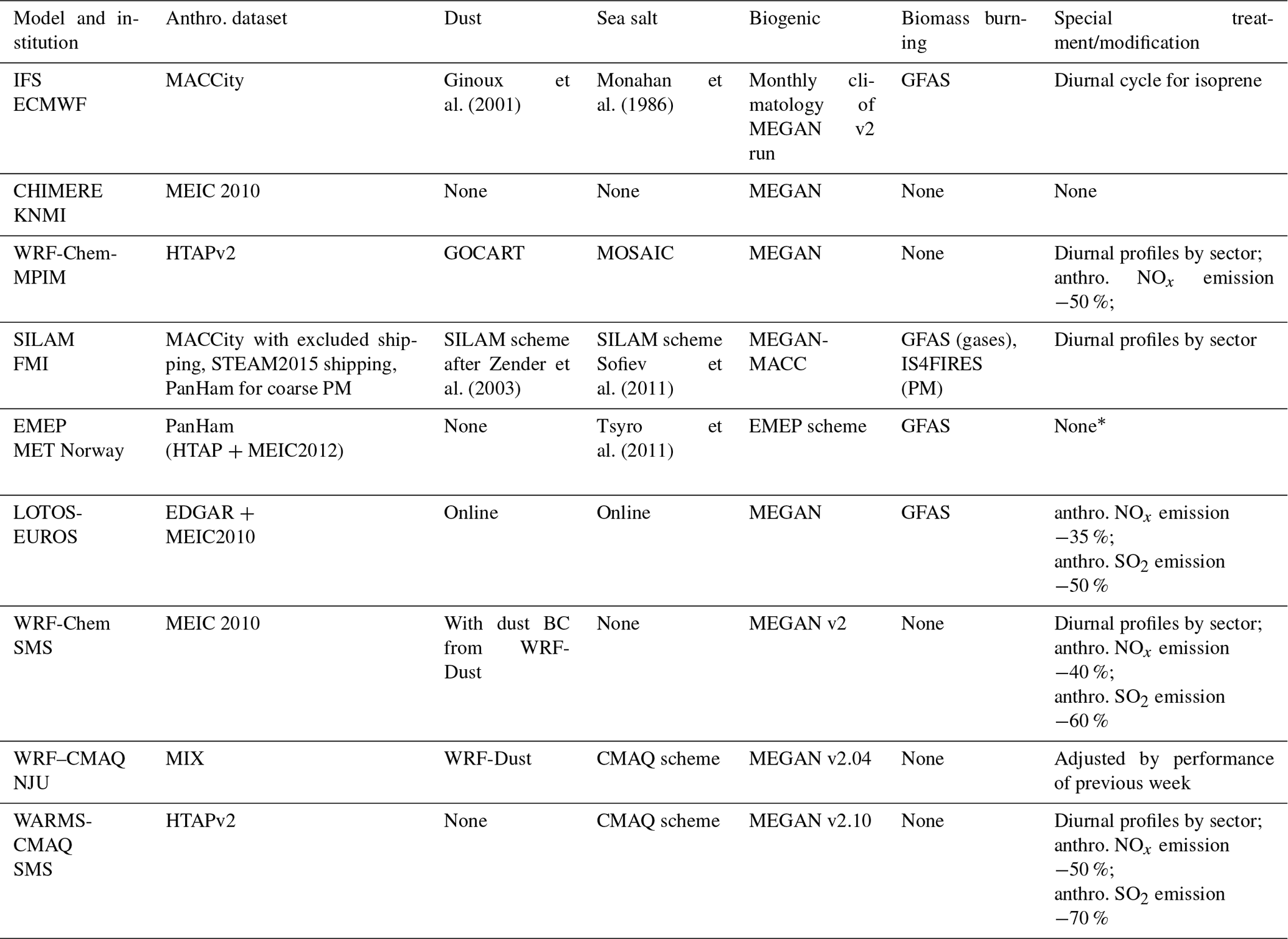
In the following subsections, each of the nine participating models will be described. Table 2a–b present the key characteristics of each model involved in the intercomparison, and Table 3 summarizes the emissions adopted in each model.
2.1 IFS
IFS is ECMWF's global numerical weather prediction system. As part of the past series of European projects MACC and now of CAMS, IFS has been developed to represent optionally chemical processes in the troposphere and in the stratosphere. Flemming et al. (2015) provide a detailed description of the modeling of chemical processes in the IFS, and Inness et al. (2015) describe the data assimilation aspects.
For the work presented here, the version of IFS used is Cycle 43R1 (see documentation at https://www.ecmwf.int/en/forecasts/documentation-and-support/changes-ecmwf-model/ifs-documentation, last access: 7 December 2018). The model is run globally at a resolution of T511 (about 40 km) on the horizontal and with 60 levels on the vertical extending up to the top of the stratosphere. The chemical package used originates from the TM5 chemistry and transport model (Huijnen et al., 2010). It has been fully integrated into the IFS code and comprises 54 tracers and 120 reactions focusing on tropospheric-ozone–CO–NMVOC–NOx chemistry. In the configuration used here, stratospheric ozone is modeled with a simple linearized scheme. Aerosols are represented using the scheme described by Morcrette et al. (2009), which includes five species: dust, sea salt, black carbon, organic carbon, and sulfates. Tracers are transported using the semi-Lagrangian scheme available in IFS with a mass fixer activated in order to minimize mass nonconservation.
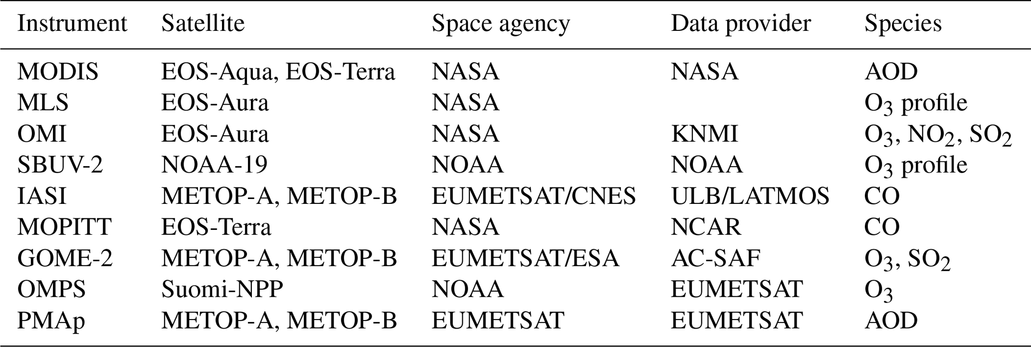
During the study period, IFS has been run twice daily (5-day forecasts) assimilating a range of satellite chemical data on top of the full list of meteorological satellite and non-satellite data that ECMWF uses for its medium-range weather forecasts. Table 1 indicates the satellite data streams actively assimilated for the experiments presented here. As a result, IFS forecasts benefit from all these observations to afford a realistic representation of large scales for weather parameters as well as, to some extent, for chemical variables (species assimilated).
IFS used the MACCity emission dataset updated for the year 2017. Biogenic emissions of volatile organic compounds (VOCs) were taken from a climatology of a multiyear Model of Emissions of Gases and Aerosols from Nature (MEGAN) simulation. Daily emissions from biomass burning were derived from satellite retrieval of fire radiative power (FRP) from the MODIS instruments by the Global Fire Assimilation System (GFAS; Kaiser et al., 2012). The observed fire emissions from the day before the forecast start are used for all 5 days of the forecast. Desert dust and sea salt emissions were simulated online for each time step based on the IFS meteorological fields and the land use.
As part of CAMS, the chemical configuration of IFS benefits from routine detailed evaluations. Validation reports are produced quarterly and can be found here: http://atmosphere.copernicus.eu/quarterly_validation_reports (last access: 7 December 2018). The report for the period March–May 2017 provides insight on the overall performance of the runs that are also presented here. Further information about the IFS code can be obtained from Vincent-Henri Peuch (vincent-henri.peuch@ecmwf.int) and on the website https://www.ecmwf.int/en/about/what-we-do/environmental-services/copernicus-atmosphere-monitoring-service (last access: 7 December 2018).
Table 1Satellite data streams (atmospheric composition variables only) assimilated in IFS.
2.2 CHIMERE
CHIMERE is a regional chemistry transport model used for analysis, scenarios, and forecast (Menut et al., 2013a). When used in the forecast mode, the model provides local-scale information (to be compared with data from numerous air quality networks) or regional-scale information (e.g., the French PREV'AIR and the CAMS systems). CHIMERE is an open-source model, freely distributed at http://www.lmd.polytechnique.fr/chimere/ (last access: 7 December 2018). In this version, CHIMERE is used in off-line mode at a spatial resolution of 0.25∘ (about 25 km). It is forced by pre-calculated hourly meteorological fields for the dynamics and by several emissions fluxes for the chemistry. The emissions are pre-calculated or online estimated in the model with anthropogenic emissions (MEIC 2010), biogenic emissions with the online MEGAN (Guenther et al., 2006), mineral dust (Menut et al., 2013b), and biomass burning emissions (Turquety et al., 2014). The gas-phase chemistry is calculated using the MELCHIOR2 mechanism, and the aerosols are represented using a distribution of 10 bins, from 40 nm to 40 µm to describe both number and mass well. The chemical boundary conditions are provided by the LMDz-INCA model for gas and particles (Szopa et al., 2009), except for mineral dust, which is extracted from global GOCART simulations (Ginoux et al., 2001). Further information about the implementation of the model for air quality forecasts in China can be obtained from Ronald van der A (avander@knmi.nl) at KNMI and on the website http://www.lmd.polytechnique.fr/chimere/CW-download.php (last access: 7 December 2018).
2.3 WRF-Chem-MPIM
WRF-Chem is a mesoscale non-hydrostatic meteorological model (Skamarock et al., 2008) coupled “online” with chemistry that simultaneously predicts meteorological and chemical components of the atmosphere (Grell et al., 2005; Fast et al., 2006).
The model version used at the Max Planck Institute for Meteorology (MPIM), WRF-Chem-MPIM, is based on version 3.6.1 of the WRF-Chem model coupled to the gas-phase chemistry and the aerosol microphysics schemes provided by the Model for Ozone and Related Chemical Tracers (MOZART-4; Emmons et al., 2010) and the Model for Simulating Aerosol Interactions and Chemistry (MOSAIC; Zaveri et al., 2008), respectively. Aerosol sizes are represented by four consecutive bins, and the formation of secondary organic aerosol (SOA) from anthropogenic precursors is parameterized according to Hodzic and Jimenez (2011).
Two nested model domains with horizontal resolutions of 60 km (Asian continent from India to Japan) and 20 km (eastern China), respectively, are implemented. The vertical grid is composed of 51 levels extending from the surface to 10 hPa (∼30 km). A more complete description of the selected physical and chemical options is provided in the WRF and in the WRF-Chem user's guides under http://www2.mmm.ucar.edu/wrf/users/docs/user_guide_V3.6/ARWUsersGuideV3.6.1.pdf (last access: 7 December 2018) and https://ruc.noaa.gov/wrf/wrf-chem/Users_guide.pdf (last access: 7 December 2018).
The WRF-Chem-MPIM model forecasts are initialized and forced at the lateral boundaries every day by 6-hourly meteorological analysis data from the NCEP Global Forecast System (GFS) at 0.5∘ resolution. For the chemical and aerosol species, 6-hourly datasets are provided by the global operational forecasting system implemented within the Copernicus Atmospheric Monitoring Service project (Flemming et al., 2015). More information on the model's configuration can be obtained from Idir Bouarar (idir.bouarar@mpimet.mpg.de) at the Max Planck Institute for Meteorology and on the website http://www2.mmm.ucar.edu/wrf/users/downloads.html (last access: 7 December 2018).
2.4 SILAM
FMI uses the SILAM version 5.5 (Sofiev et al., 2015a, b). SILAM includes a meteorological preprocessor for diagnosing the basic features of the boundary layer and the free troposphere from the meteorological fields provided by various meteorological models (Sofiev et al., 2010). The dry-deposition scheme for particles is described in Kouznetsov and Sofiev (2012). The surface resistance model for gases is based on a modified Wesely scheme (Wesely, 1989).
The gas-phase chemistry was simulated with CBM-IV, with reaction rates updated according to the recommendations of IUPAC (http://iupac.pole-ether.fr, last access: 7 December 2018) and JPL (http://jpldataeval.jpl.nasa.gov, last access: 7 December 2018) and the terpenes oxidation added from the 2005 Carbon Bond (CB05) chemical mechanism reaction list (Yarwood et al., 2005). The sulfur chemistry and secondary inorganic aerosol formation is computed with an updated version of the DMAT scheme (Sofiev, 2000), and secondary organic aerosol formation is computed with the volatility basis set (VBS; Donahue et al., 2006), with the volatility distribution of anthropogenic organic carbon (OC) taken from Shrivastava et al. (2011).
The MACCity land-based emissions are used together with the Ship Traffic Emission Assessment Model (STEAM). The simulations include sea salt emissions as in Sofiev et al. (2011), biogenic VOC emissions as in Poupkou et al. (2010), wild land fire emissions as in Soares et al. (2015), and desert dust.
The grid cell size was roughly 15 km × 10 km (0.125∘ × 0.125∘) covering the whole of China, India, Japan, and several countries of Southeast Asia (7∘ N, 67∘ E) – (54∘ N, 147∘ E). The Asian forecasts are nested into the SILAM global air quality forecasts (http://silam.fmi.fi, last access: 7 December 2018), from where they take lateral and top boundary conditions. The initial conditions for each run are taken from the previous day's forecast or, in case of failure, from global computations. Detailed information about the SILAM modeling system can be obtained from Mikhail Sofiev (Mikhail.Sofiev@fmi.fi) and from Rostislav Kouznetsov (rostislav.kouznetsov@fmi.fi) and on the website of the Finnish Meteorological Institute (http://silam.fmi.fi/).
2.5 EMEP
EMEP/MSC-W (hereafter referred to as “EMEP model”) is a 3-D Eulerian chemical transport model described in detail in Simpson et al. (2012). Although the model has traditionally been aimed at European simulations, global modeling has been possible for many years (Jonson et al., 2010; Wild et al., 2012). The EMEP configuration for the present study covers the east Asian domain (15–55∘ N × 90–135∘ E) with a horizontal resolution of 0.1∘ × 0.1∘ (longitude–latitude). The model uses 20 vertical levels defined as sigma coordinates. The 10 lowest levels are within the planetary boundary layer (PBL), and the top of the model domain is at 100 hPa.
Particulate matter (PM) emissions are split into elementary carbon, organic matter (OM) (here assumed inert), and the remainder, for both fine and coarse PM. The OM emissions are further divided into fossil fuel and wood-burning compounds for each source sector. As in Bergström et al. (2012), the OM / OC ratio of emissions by mass is assumed to be 1.3 for fossil-fuel sources and 1.7 for wood-burning sources. The model also calculates windblown dust emissions from soil erosion. Secondary PM2.5 aerosol consists of inorganic sulfate, nitrate, ammonium, and SOA; the latter is generated from both anthropogenic and biogenic emissions (anthropogenic SOA and biogenic SOA, respectively), using the VBS scheme detailed in Bergström et al. (2012) and Simpson et al. (2012).
Model updates since Simpson et al. (2012), resulting in EMEP model version rv4.9 as used here, have been described in Simpson et al. (2016) and references cited therein. The main changes concern a new calculation of aerosol surface area, revised parameterizations of N2O5 hydrolysis on aerosols, additional gas-aerosol loss processes for O3, HNO3, and HO2, a new scheme for ship NOx emissions, and the use of new maps for global leaf area (used to calculate biogenic VOC emissions) – see Simpson et al. (2015) for details. The EMEP model, including a user guide, is publicly available as open-source code at https://github.com/metno/emep-ctm (last access: 7 December 2018). For more details, please contact Michael Gauss (michael.gauss@met.no).
The EMEP forecasts are driven by 3-hourly meteorological forecast data from the ECMWF IFS model at 0.1∘ resolution. As for WRF-Chem, 6-hourly datasets for the chemical and aerosol species are provided by the global operational forecasting system implemented within the Copernicus Atmospheric Monitoring Service project.
2.6 LOTOS-EUROS
LOTOS-EUROS is a three-dimensional regional chemistry transport model for simulation of trace gases and aerosol concentrations in the boundary layer. Meteorological input is obtained from an off-line model, in this study from ECMWF. The model is of intermediate complexity allowing long-term model simulations. For a detailed model description, we refer to Manders et al. (2017) and references therein.
In this study LOTOS-EUROS version 1.10 was used to simulate air quality over China. The configuration is described by Timmermans et al. (2017), who adopted this version of the model to investigate the origin of fine particulate matter across China using a source apportionment technique. Through a one-way nesting procedure a simulation over east China was performed on a resolution of 0.25∘ longitude by 0.125∘ latitude, approximately 21 km by 15 km. This domain is nested in a larger domain covering China almost entirely with a resolution of 1∘ longitude by 0.5∘ latitude, approximately 84 km by 56 km. Chemical boundary conditions for the coarse resolution domain were taken from the CAMS global modeling framework (Flemming et al., 2015) and include trace gasses and aerosols. In the vertical, the model used a boundary layer approach with five layers: a surface layer of 25 m, a well-mixed boundary layer, two reservoir layers, and a layer for the free troposphere. The boundary layer height therefore defines the vertical structure of the model, and is here taken from the meteorological input. More details about the code can be obtained by contacting Renske Timmermans (renske.timmermans@tno.nl) at TNO or by consulting the website https://lotos-euros.tno.nl/ (last access: 7 December 2018).
2.7 WRF-Chem-SMS
WRF-Chem-SMS hosted at the Shanghai Meteorological Service is based on WRF-Chem (Grell et al., 2005) version 3.2. The Regional Acid Deposition Model version 2 (RADM2; Chang et al., 1989) is used to represent gas-phase chemistry. ISORROPIA II is implemented to treat thermodynamic equilibrium for inorganic aerosols (Fountoukis and Nenes, 2007), and the Secondary ORGanic Aerosol Model (SORGAM) (Schell et al., 2001) is used to parameterize secondary organic aerosol formation. A Madronich TUV scheme is applied for photolysis (Madronich and Flocke, 1999; Tie et al., 2003). The model domain covers the eastern region of China with horizontal resolutions of 6 km and 28 vertical layers. Biogenic emissions are calculated online using MEGAN (Guenther et al., 2012). The multi-resolution emission inventory for China (MEIC inventory, http://www.meicmodel.org/ (last access: 7 December 2018); Li et al., 2014; Liu et al., 2015) for the year 2010 is used to represent anthropogenic emissions.
The modeling system is initialized and forced at the lateral boundaries every day by 6-hourly data from the NCEP GFS at 0.5∘ resolution. For chemical species, a previous modeling result is used for initial conditions. MOZART-4 historic data are employed as the gaseous chemical lateral boundary, and a real-time forecast of dust from the WRF-Dust model is employed as a dust lateral boundary every 6 h. More detailed information can be found in Zhou et al. (2017) and by contacting Jianming Xu (metxujm@163.com) at the Shanghai Meteorological Service.
2.8 WRF–CMAQ
A regional air quality operational forecasting system was developed at Nanjing University, China, on the basis of the WRF–CMAQ model. The versions adopted for the WRF (Weather and Forecasting) and CMAQ (Community Multiscale Air Quality) models are V3.5 and V4.7.1, respectively. Two nested domains with horizontal resolutions of 36 and 12 km are adopted for the forecasts. The outer domain covers the entire continental region of China as well as surrounding countries in east Asia. The inner domain mainly focuses on the densely populated area of eastern China. The number of grid points adopted for the WRF model are 170×130 and 202×226, respectively with 51σ layers in the vertical (12 layers below 1.5 km a.g.l.) between the surface and the model top at 50 hPa. The CMAQ model is applied to the same domains but with three grid cells removed at each lateral boundary of the WRF domains. Overall, 15 vertical layers are selected from the 51 WRF layers, including about 8 layers in the boundary layer and 7 layers in the free troposphere.
Anthropogenic emissions are supplied off-line from the MIX inventory (Li et al., 2017). Terrestrial biogenic emissions are calculated off-line using MEGAN v2.04 (Guenther et al., 2006). Sea salt emissions are incorporated into the AERO4 aerosol module and calculated online in CMAQ. Windblown dust is derived online from the WRF-Dust model. Open biomass burning emissions are not considered here. It should be noted that the anthropogenic emissions are not fixed in this system but are automatically adjusted every week according to the system performance in the past week. The adopted scaling factors are determined from the deviation between the weekly averaged calculated and observed concentrations of SO2, NOx, CO, PM2.5, and PM10 in 334 Chinese prefectures.
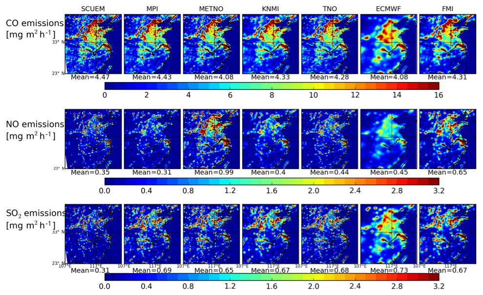
Figure 1Surface emissions of CO, NO, and SO2 (mg m−2 h−1) adopted by the different models (average for the period 1–14 March 2017). Note that the SCUEM emissions are those used in the WRF-Chem-SMS model.
The system provides a forecast every day for the next 192 h. The NCEP GFS's products at 00:00 UTC are used for the initial and boundary conditions of the WRF model with a resolution of 0.5∘ and with a 3 h interval. For the CMAQ model, the boundary conditions are created using ideal profiles, and the chemical initial fields are initialized from the previous forecasting. In addition, hourly averaged observed concentrations of SO2, NO2, CO, O3, PM2.5, and PM10 from 1415 national control air-quality-monitoring sites are assimilated into the initial fields using an optimal interpolation method (Lorenc, 1981). More information on the code can be obtained from Fei Jiang (jiangf@nju.edu.cn) at Nanjing University. Information on WRF–CMAQ is also available on the website http://carbon.nju.edu.cn/cn/ (last access: 7 December 2018) and https://www.epa.gov/cmaq/cmaq-models-0 (last access: 7 December 2018).
2.9 WARMS-CMAQ
The Community Multiscale Air Quality (CMAQ) model is a 3-D Eulerian chemical transport model that explicitly simulates emissions, gas-phase, aqueous, and mixed-phase chemistry, advection and dispersion, aerosol thermodynamics and physics, and wet and dry deposition. A detailed description and an evaluation of the CMAQ model are available in the papers by Byun and Schere (2006), Foley et al. (2010), and Appel et al. (2017). Several studies have applied the CMAQ model to study the air quality in China. For example, Zheng et al. (2015) used the WRF–CMAQ model to study the impact of heterogeneous chemistry during the January 2013 haze episode. Hu et al. (2016) performed a 1-year retrospective simulation using the WRF–CMAQ model to study the O3 and particulate matter formation with a detailed evaluation. Here the CMAQ version 5.0.2 is adopted and includes the CB05 (Yarwood et al., 2005) to represent the gas-phase chemistry. The fifth-generation modal CMAQ aerosol model (aero5) is adopted to formulate the aerosol chemistry and dynamics (Carlton et al., 2010).
In this version, CMAQ is used in an off-line mode. It is forced by pre-calculated hourly meteorological fields for the dynamics and by several emissions fluxes for the chemistry. Meteorology fields that drive chemical transport are produced by the SMS-WARMS. The SMS-WARMS has been extensively evaluated and provides weather predictions in eastern China. The modeling domain consists of 760 by 600 horizontal grids at 9 km resolution, with 51 layers in the vertical. As a subdomain of the SMS-WARMS run, the CMAQ domain consists of 430 by 370 horizontal grid cells at 9 km resolution. In the vertical, 26 layers are applied.
The anthropogenic emissions are based on the monthly HTAP v2 dataset (http://edgar.jrc.ec.europa.eu/htap_v2/, last access: 7 December 2018) (Janssens-Maenhout et al., 2015) for the year 2010. As suggested by operational forecasting results, the HTAP NOx, SO2 emissions are adjusted to account for rapid economic growth in the region. Biogenic emissions are estimated by MEGAN version 2.10 (Guenther et al., 2012). Currently, dust and biomass burning emissions are not included.
For the SMS-WARMS model forecasts, the NCEP GFS output at 0.5∘ is used as a background for the ADAS data assimilation scheme, which ingests many local observations (e.g., radar and buoys), and to provide lateral boundary conditions. The chemical boundary conditions are currently based on the default vertical profiles of gaseous species and aerosols in CMAQ that represent clean-air conditions. For more details, please contact Ying Xie (yxie33@outlook.com) at the Shanghai Meteorological Service. The CMAQ code available on the U.S. EPA modeling site https://github.com/USEPA/CMAQ/ (last access: 7 December 2018).
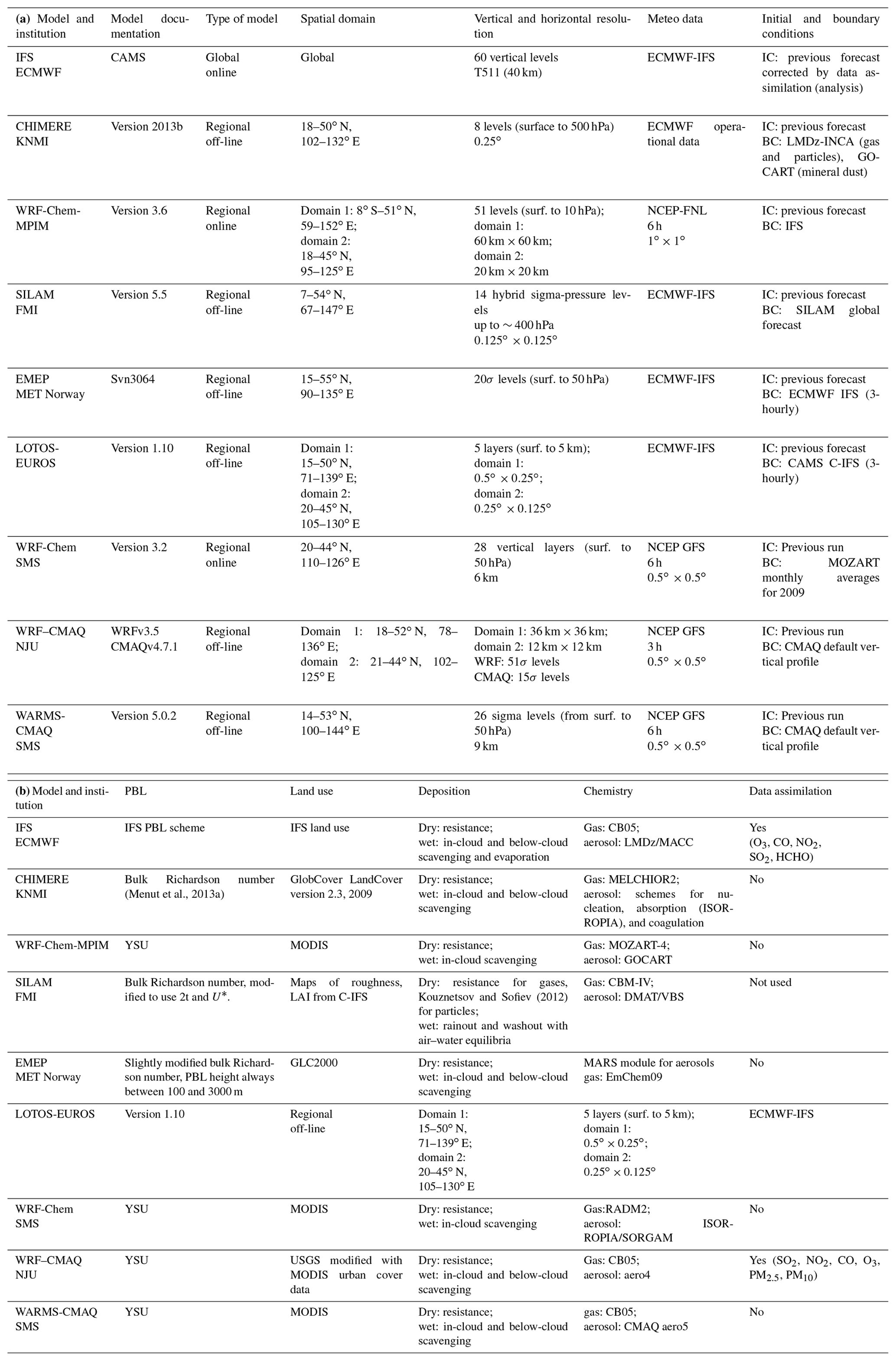
The choice of the adopted surface emissions for primary chemical species has a significant influence on the atmospheric concentrations calculated for these species and for related secondary pollutants. In this intercomparison exercise, the different groups involved have adopted their preferred anthropogenic emissions based on published inventories such as MEIC (Li et al., 2014; Liu et al., 2015), MACCity (Granier et al., 2011), EDGAR (Emission Database for Global Atmospheric Research; Muntean et al., 2014; Crippa et al., 2016), and HTAP (Janssens-Maenhout et al., 2015). An inventory developed specifically for the Panda project called PanHam has been obtained by combining information from the MEIC and HTAP inventories. Each model uses its own formulation for dust mobilization or seal salt emissions. In most cases, the biogenic emissions are derived online or off-line from MEGAN (Guenther et al., 2006, 2012). Table 3 provides more details about the specified emissions and Fig. 1 shows the mean distribution of the anthropogenic emissions for CO, NO, and SO2 adopted by different models during the period 1–14 March 2017. In the case of carbon monoxide, the adopted emissions are relatively similar in all models with mean emissions ranging from 4.0 to 4.6 mg m−2 h−1. In the case of nitric oxide, however, there are substantial differences with mean emissions ranging from 0.31 mg m−2 h−1 (WRF-Chem-MPIM) to 0.99 mg m−2 h−1 (EMEP) but with values around 0.30–0.45 mg m−2 h−1 used by most models. For sulfur dioxide, produced primarily from coal combustion, the adopted values range from 0.31 mg m−2 h−1 (WRF-Chem-SMS) to 0.73 mg m−2 h−1 (IFS) but with values around 0.67 mg m−2 h−1 adopted in most models. The low values adopted for WRF-Chem-SMS reflect the likely impact of the recent measures taken in China to limit the emissions from coal burning facilities.
Emission inventories that are currently available to the modeling community usually account for anthropogenic emissions for the years 2010 to 2012 and hence do not account for the substantial reduction in the emissions that took place since around 2014 as a result of actions taken by the Chinese authorities. The lower emission values adopted by several models may therefore be more realistic for providing chemical weather forecasts in 2017.
Table 3Adopted emissions.
* None during the intercomparison exercise. Since summer 2017, however, the NOx
emissions have been reduced by 35 % in this particular model. The present version
of the model also calculates windblown dust emissions from soil erosion.
As stated above, the MarcoPolo–Panda system is used operationally to provide daily forecasts of air quality in eastern China. In its present configuration (Fig. 2), the system is based on nine models, which are executed independently on the computing system available at each respective partner institution. The outputs of the models are locally processed and the surface concentrations of the key chemical species are forwarded to a central database operated by the KNMI. Ensemble mean and median concentrations are derived and, in addition to the forecasts from individual models, are posted on a dedicated website (http://www.marcopolo-panda.eu/, last access: 7 December 2018) and Chinese mirror site (http://116.62.195.108/, last access: 7 December 2018). For the 37 Chinese cities with a population above 3 million in 2010, the predicted concentration values of ozone, NO2, PM2.5, and PM10 are compared each hour to local measurements reported by the Chinese monitoring network (http://pm25.in/, last access: 7 December 2018). Observations for each city represent the mean of several measurements performed within one city (usually 5–12 stations). The data are averaged to city-center coordinates.
We start by presenting a few examples of randomly selected forecasts as provided by the MarcoPolo–Panda system to illustrate the diversity among the models and the differences obtained under different situations. The performance of each individual model varies from day to day because it strongly depends on the individual weather forecast (meteorological situation, cloudiness, precipitation, etc.) that is adopted to simulate transport, photochemistry, and deposition. Therefore, this first description of model forecasts does not provide reliable information on the accuracy of the forecasts provided by the different models included in the ensemble.
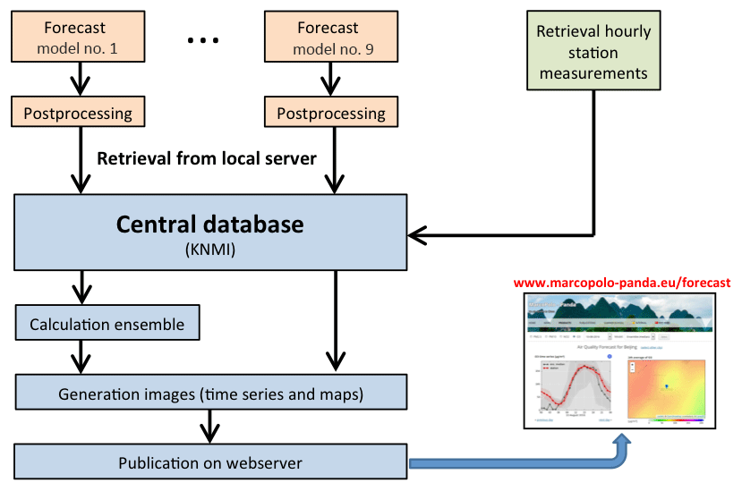
Figure 2Structure of the operational multi-model forecast system with the nine model components. Postprocessed forecasts for the next 3 days provided by each model are sent to a central database maintained by the Royal Netherlands Meteorological Institute (KNMI). Ensemble medians and means are calculated and information (predicted daily variations in surface concentrations for 37 major Chinese cities, and maps of predicted diurnal mean surface concentrations) and are posted on http://www.marcopolo-panda.eu/forecast (last access: 7 December 2018). Users in China are redirected to the mirror website maintained by SMS (http://116.62.195.108/, last access: 7 December 2018). The forecasts are compared with the median and mean observations provided by monitoring stations at different locations of the 37 cities.
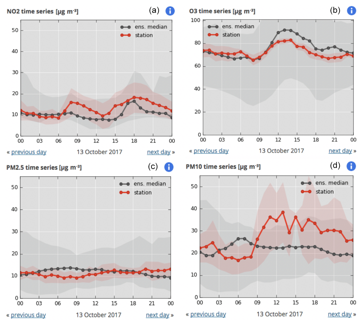
Figure 3Median concentrations of NO2 (a), ozone (b), PM2.5 (c), and PM10 (d) predicted for the city of Xiamen on 13 October 2017 (black curve) and compared with the measured values (red curves). The dispersion of the forecasts by the individual models belonging to the ensemble is shown by the grey range, and the dispersion of the measured values at different stations in the city are depicted by the pink band.
The first example presents a relatively successful forecast made for the coastal city of Xiamen in southeast China on 13 October 2017. The panels in Fig. 3 show the excellent agreement in the case of NO2, ozone, and PM2.5, suggesting that the median values derived from the individual models capture well the features associated with the meteorological situation, atmospheric transport, and the emissions in the region on that particular day. The situation corresponds to very clean conditions, with PM2.5 and NO2 concentrations of the order of 10–15 µg m−3. The predicted ozone concentration ranges from 70 to 90 µg m−3 (35 to 45 ppbv). Interestingly, however, the predicted PM10 concentrations are underestimated during most of the day. The model predicts concentrations close to 20–25 µg m−3, while the measurements indicate that the concentration reached values as high as 30–40 µg m−3. The presence on 13 October of a strong wind flow in the strait between mainland China and Taiwan and associated with the Khanun tropical depression present on this particular day west of the Philippines was likely a source of elevated sea salt emissions and dust mobilization that may not have been properly captured by the models. Under such strong meteorological disturbance, the forecast could be strongly resolution dependent.
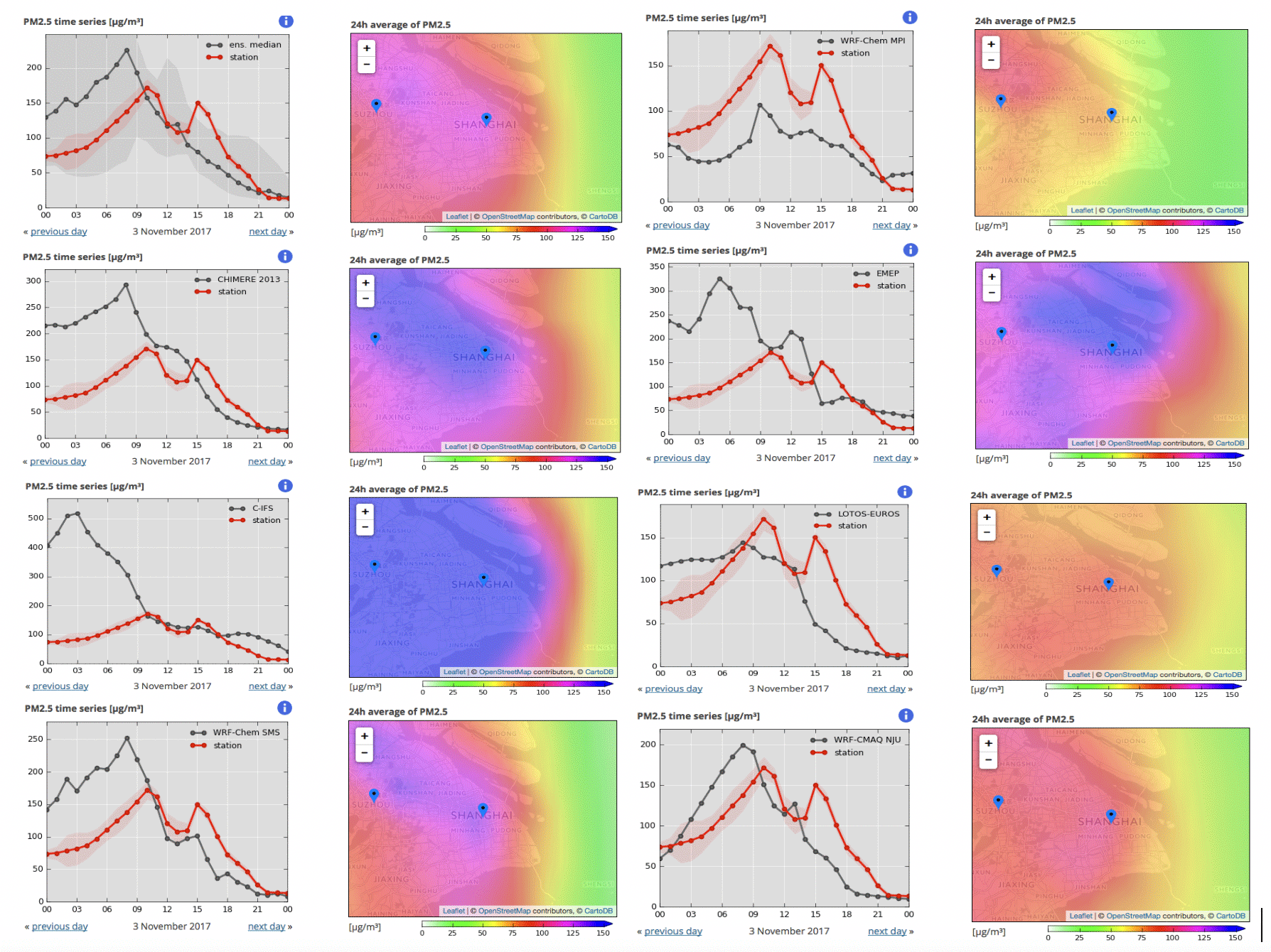
Figure 4Forecast by different models of PM2.5 concentration during a polluted day in Shanghai on 3 November 2017. The graph in the top panel of the first column represents the median concentration, and the individual forecasts provided by CHIMERE, IFS, WRF-Chem-SMS, WRF-Chem-MPIM, EMEP, LOTOS-EUROS, and WRF–CMAQ are shown by the other panels. Measured concentrations are represented by the red curves and model concentrations by the black curves.
The second example of predictions (Fig. 4) refers to the forecast of PM2.5 in Shanghai on a relatively polluted day (3 November 2017). All models predict the presence of relatively high concentrations over land (diurnal mean values of typically 100–150 µg m−3) with a steep negative gradient towards the Chinese sea, where the concentrations are of the order of only 25–40 µg m−3. Observations made at different stations in this urban area show the occurrence of two successive concentration peaks: one around 09:00–10:00 with concentrations reaching about 180 µg m−3 and the second one at 15:00–16:00 with concentrations as high as 150 µg m−3. The ensemble mean forecast system predicts the occurrence of a single peak at about 07:00 with a PM2.5 concentration of about 220 µg m−3. The forecast shows a gradual decrease in the concentration during the afternoon that is in good agreement with the observation. The occurrence of the second peak in the afternoon, however, is missed by the ensemble prediction, even though a peak appears in some of the individual model calculations (WRF-Chem SMS, EMEP, and WRF–CMAQ) but often a few hours before it was actually detected by the monitoring stations. An inspection of the forecasts by the different models highlights the diversity in the model results. IFS, CHIMERE, WRF-Chem-SMS, and EMEP overestimate the PM2.5 concentrations before midday, while they provide values in good agreement with the observations in the afternoon and evening. WRF-Chem-MPIM underestimates the concentrations during the entire day. LOTOS-EUROS as well as WRF–CMAQ provide values that are in fair agreement with the observations in the morning but underestimate the concentrations in the afternoon.
A third example (Fig. 5) refers to the predicted concentration of PM2.5 on 25 October 2017 in Beijing. In this particular case, the ensemble forecast system predicts the occurrence of a rather polluted day with stagnant air and high concentrations of aerosol particles over Beijing as a band stretching from the southwest to the northeast. The median concentration predicted for this day is close to 200 µg m−3 but is a factor of 2 higher than the observation. Most individual models produce this band of high PM2.5 concentrations with the exception of the WRF-Chem-MPIM model that shows moderate levels of pollution with an aerosol cloud localized in the urban area of Beijing. An examination of the results provided by the individual models again shows large differences. Some models (CHIMERE, EMEP, LOTOS-EUROS, WRF-Chem-MPIM) calculate a slow and rather steady concentration increase during the day, while other models (WRF-Chem-SMS, WARMS-CMAQ-SMS, SILAM, and IFS) exhibit some irregular variations during the day. Most models overestimate the PM2.5 concentrations except for LOTOS-EUROS and WRF-Chem-MPIM, which predict concentrations with the same order of magnitude as the observations at the monitoring stations. The last illustrative example refers to the forecast of nitrogen oxides and ozone in the Shanghai area on 31 October 2017 (Fig. 6a, b, and c). All models show that the NO2 concentrations are highest in the boundary layer of the urban areas, even though the calculated values may be different from model to model, and the dispersion of the species away from the urban centers may also be uneven. In all cases, predicted values above the ocean are very low, i.e., less than a few µg m−3. A band of high NO2 concentrations extends from Shanghai in the northwest direction.
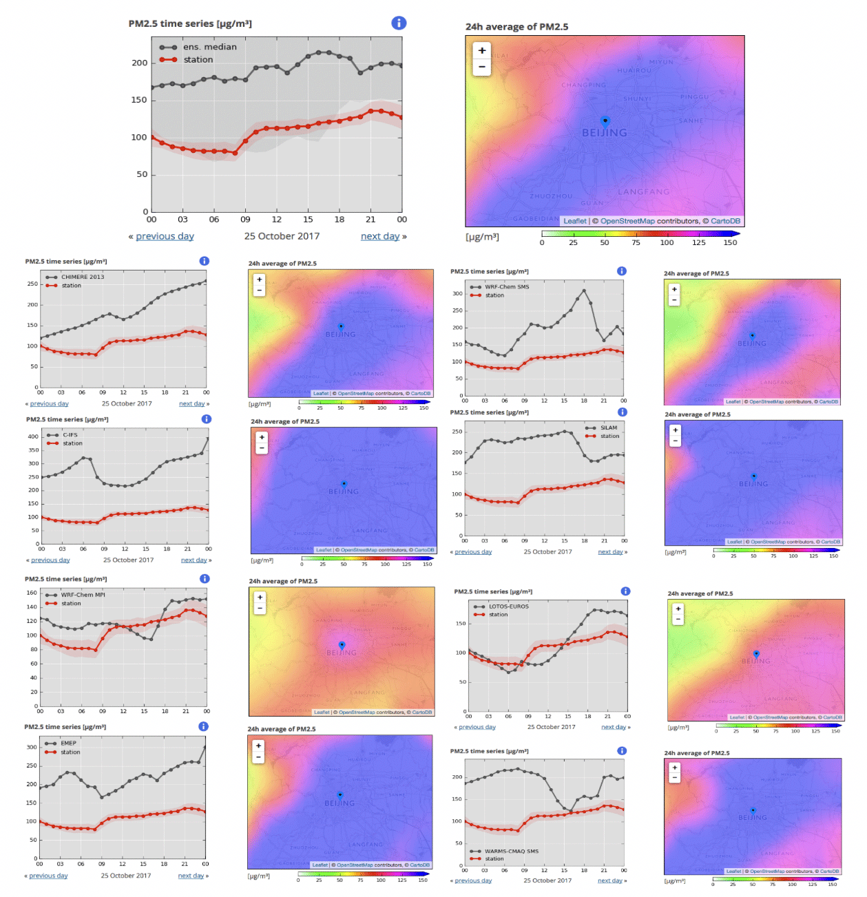
Figure 5Diversity of PM2.5 forecasts in Beijing on 25 October 2017 by several models included in the ensemble of the MarcoPolo–Panda prediction system. The ensemble median is shown by the top panels, and the individual forecasts provided by CHIMERE, IFS, WRF-Chem-MPIM, EMEP, WRF-Chem-SMS, SILAM, LOTOS-EUROS, and WARMS-CMAQ-SMS are shown by the other panels. Measurements are in red and model data in black.
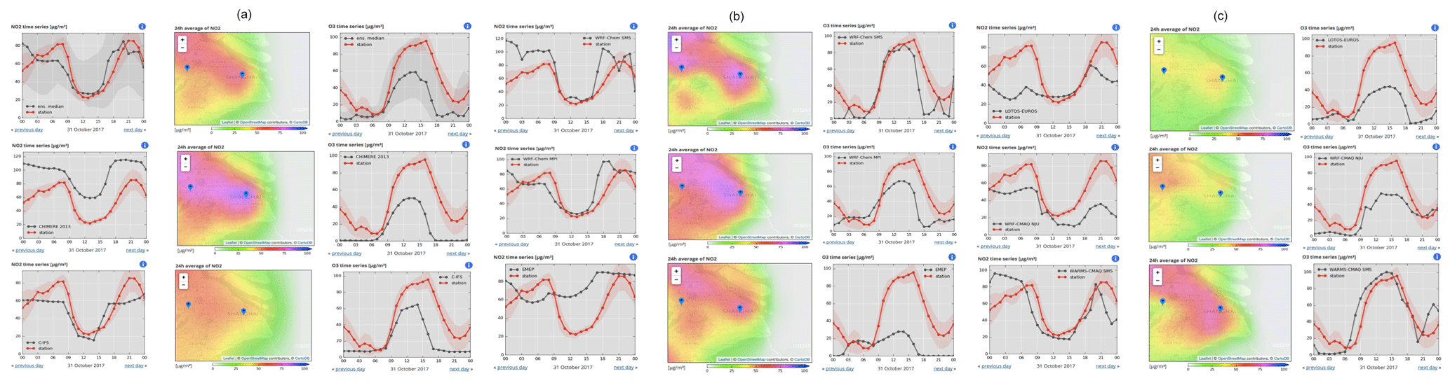
Figure 6(a) Diversity in the NO2 and ozone forecasts made for Shanghai on 31 October 2017 as highlighted by the predictions from several models included in the ensemble of the MarcoPolo–Panda system. The left and right columns show the diurnal variation in the predicted (black) and observed (red) NO2 and ozone concentrations (µg m−3), respectively. The center column presents the geographical distribution in the vicinity of Shanghai of the diurnal average predicted for the NO2 concentration. The ensemble median is shown in the top row, and two individual forecasts as provided by CHIMERE and IFS are shown in the middle and lower rows. (b) Same as in (a) but for the individual forecasts from WRF-Chem-SMS, WRF-Chem-MPIM, and EMEP. (c) Same as (a) but for the individual forecasts from LOTOS-EUROS, WRF–CMAQ, and WARMS-CMAQ.
The median values of NO2 in the city (Fig. 6a) are in good agreement with the observed values, with nighttime concentrations on the order of 60–80 µg m−3 and substantially lower values during daytime resulting from the photolysis of the molecule by solar radiation. A minimum concentration of 25 µg m−3 is reached around noon.
The diurnal variation in NO2 is well captured by most models, in particular by CHIMERE (although the absolute values are too low), IFS, WRF-Chem-SMS, WRF-Chem-MPIM, and WARMS-CMAQ-SMS. The diurnal variation is somewhat underestimated in EMEP, LOTOS-EUROS, and WRF–CMAQ.
The ozone concentration (Fig. 6a–c) also exhibits a strong diurnal variation that, to a large extent, mirrors the NO2 variation. Measurements show a maximum value of nearly 100 µg m−3 reached at 15:00 and low nighttime concentrations (typically 10–30 µg m−3). The median concentrations, provided by the ensemble forecast system (Fig. 6a), are characterized by a similar diurnal variation but with lower amplitude. The concentration reaches its maximum at 14:00, but the value of this maximum is only equal to 60 µg m−3. The values predicted for the night are generally somewhat smaller than the observation, with values of the order of 5–10 µg m−3.
In the case of ozone, differences between model forecasts are again substantial. The maximum concentration values in the early afternoon are 50 µg m−3 for CHIMERE, 62 µg m−3 for IFS, 85 µg m−3 for WRF-Chem-SMS, 65 µg m−3 for WRF-Chem-MPIM, 30 µg m−3 for EMEP, 42 µg m−3 for LOTOS-EUROS, 57 µg m−3 for WRF–CMAQ, and 100 µg m−3 for WARMS-CMAQ-SMS.
We now present an intercomparison of most of the models included in the operational MarcoPolo–Panda System. The participants to this intercomparison examined in detail the daily forecasts performed for the month of March 2017 with particular emphasis on the results obtained during the first 2 weeks of the month.
In the following sections, we present selected chemical fields derived by the different models that participated in the comparison exercise and highlight similarities and differences with the purpose of identifying the causes of the discrepancies between models and between models and observations. We first examine monthly mean surface concentrations obtained from a subset of the models involved in the intercomparison. We then compare the time evolution associated with the model forecasts with observations made at specific surface measurement sites and present some correlations between calculated and measured concentrations at these sites.
5.1 Comparison of average fields
We first compare the March 2017 monthly mean concentrations of different chemical species calculated by seven models (IFS, LOTOS-EUROS, EMEP, SILAM, WRF-Chem-MPIM, WRF-Chem-SMS, and CHIMERE) with surface measurements reported at different sites in the eastern part of China (http://pm25.in/).
Figure 7a shows the calculated and observed surface concentrations of carbon monoxide (CO). We first note the substantial differences that exist between the individual model forecasts, probably reflecting differences in the adopted emissions or in the atmospheric production resulting from the oxidation of volatile organic compounds in the planetary boundary layer. Observations indicate that CO concentrations are generally higher than 900 ppbv, except near the southeastern coast and in the southwestern part of the country, where the values are as low as 500 to 700 ppbv. The models show considerably lower values, ranging from about 300 to 500 ppbv. The regions with the highest mean concentrations are located in the North China Plain (NCP), where values higher than 1200 ppbv are recorded. Relatively high values (close to 1000 ppbv) are also found in some urban areas (e.g., Hong Kong) near the south coast of the country.

Figure 7Monthly mean surface concentrations of (a) CO, (b) NO2, (c) ozone (ppbv), and (d) PM2.5 (µg m−3) provided for the month of March 2017 by different models: CHIMERE (no CO), IFS, WRF-Chem-SMS, SILAM, WRF-Chem-MPIM, EMEP, and LOTOS-EUROS. The monthly mean concentration values derived from observations at different monitoring stations are represented by dots in the last plot of the bottom panel. The adopted color scales are the same as the color scales adopted to represent the model results.
The models provide a rather different picture: most of them substantially underestimate the CO concentrations, in particular WRF-Chem-SMS, WRF-Chem-MPIM, EMEP, and LOTOS EUROS. Higher concentrations are derived by SILAM and IFS. These models, however, produce peak concentrations in the region of the Sichuan Basin in contrast with the observations. Only IFS reproduces the high concentrations observed in northern China, probably because in this particular model the initial conditions are constrained by assimilated observations. Clearly, the performance of the models regarding the calculation of CO concentrations is not satisfactory. The discrepancies may be attributed to an underestimation of CO emissions, to errors in the lateral boundary conditions, or indirectly to an underestimation of the emissions for primary hydrocarbons.
In the case of NO2 (Fig. 7b), the observations show that the surface concentrations are highest in the northeastern portion of China with a few urban hot spots. These patterns are reproduced well by the EMEP, SILAM, and IFS models. The other models also produce high concentrations in urban areas but with values that are lower than those provided by the monitoring stations.
The mean surface ozone concentrations derived from measurements are lowest (about 20 ppbv) in the central part of China and highest (30–40 ppbv) near the east coast (Shanghai region), the south coast, and the western part of China. Since nitrogen oxides tend to titrate ozone, the models that predict high NO2 concentrations derive the lowest ozone values (EMEP, SILAM, IFS). The high NO2 concentrations predicted by EMEP are probably related to the large emissions used as shown in Fig. 1. CHIMERE, WRF-Chem-SMS, and to a lesser extent WRF-Chem-MPIM overestimate the mean ozone concentration during March. All models, however, produce a minimum in the ozone concentrations in northeastern China, a pattern that is not visible in the observational data (Fig. 7c).
Finally, in the case of PM2.5 (Fig. 7d), the measurements suggest the presence of high concentrations (higher than 80 µg m−3) in the region between Beijing and Shanghai. High abundances of PM2.5 are derived in this region by IFS, SILAM and to a lesser extent by LOTOS-EUROS, EMEP, CHIMERE, and WRF-Chem-SMS. Interestingly, most models produce another marked hot spot in the region of the Sichuan Basin, while the observations suggest a less pronounced maximum with a more limited geographical extent.
5.2 Time evolution of median forecasts
We now focus on the time period during which the most intensive comparison between models has been performed. We first examine the time evolution of surface ozone, NO2, and PM2.5 produced by the different models for the time period ranging from 1 to 15 March 2017 and for the three large metropolitan areas: Beijing, Shanghai, and Guangzhou. In Fig. 8, we compare the median concentrations of the three species with the median values derived from the different measurements provided by the network of instruments deployed in the three cities. The median model values are represented by the red curves, while the shaded areas highlight the dispersion of the calculated concentrations around the median values.
-
Beijing. Here the predictions of the PM2.5 concentrations follow the observations very closely. Two events with relatively high aerosol loads are visible, the first one between 2 and 5 March and the second one on 11 March. In the case of NO2, the models reproduce the daily variability reported by the monitoring stations fairly well, but on average, they slightly overestimate the concentrations values. The high concentrations appearing between 2 and 5 March and between 10 and 11 March are well captured by the median of the models. Finally, the models reproduce the diurnal variability in the ozone concentrations, but they underestimate these concentrations by typically 20 µg m−3.
-
Shanghai. The calculated median concentrations of PM2.5 are in good agreement with the observations, especially between 10 and 15 March. During the first part of the simulation, the mean measured and calculated values are close, but the models produce peaks in the concentrations on 3, 6, 8, and 9 March that are higher than the observation. In the case of NO2, the agreement between calculated and measured concentrations is good. Again, the models severely underestimate the ozone concentrations.
-
Guangzhou. The median concentration of PM2.5 provided by the model is similar to the observation between 1 and 7 March. However, the model overestimates the concentrations between 7 and 11 March and underestimates them between 12 and 14 March. For NO2, the agreement between models and measurements is relatively good during the first days of the month, but the models overestimates the amplitude of the daily variability observed after 6 March. Ozone is well simulated in this particular urban area, even though the daily peaks are sometimes over- or underestimated.
5.3 Statistical errors
In order to measure the performance of the individual models involved in the present intercomparison, we have calculated statistical measures of the model results for the chosen period of 1–15 March 2017. These measures include the mean bias (BIAS), the mean normalized bias (MNMBIAS), the root mean square error (RMSE), the fractional gross error (FGE), and the correlation coefficient for ozone, NO2, and PM2.5 (Table 4). They apply to the data for the 37 cities considered in the MarcoPolo–Panda forecast system. The same statistical measures are also provided for the ensemble median.
Table 4For the period 1 to 15 March 2017, statistical measures (mean bias (BIAS), mean normalized bias (MNMBIAS), root mean square error (RMSE), FGE (fractional gross error), and correlation coefficients) calculated for the forecast of O3, NO2, and PM2.5 concentrations for all models and for the ensemble median at all stations/cities, for which the MarcoPolo–Panda Forecast is available. The correlation is based on 1-hourly data.
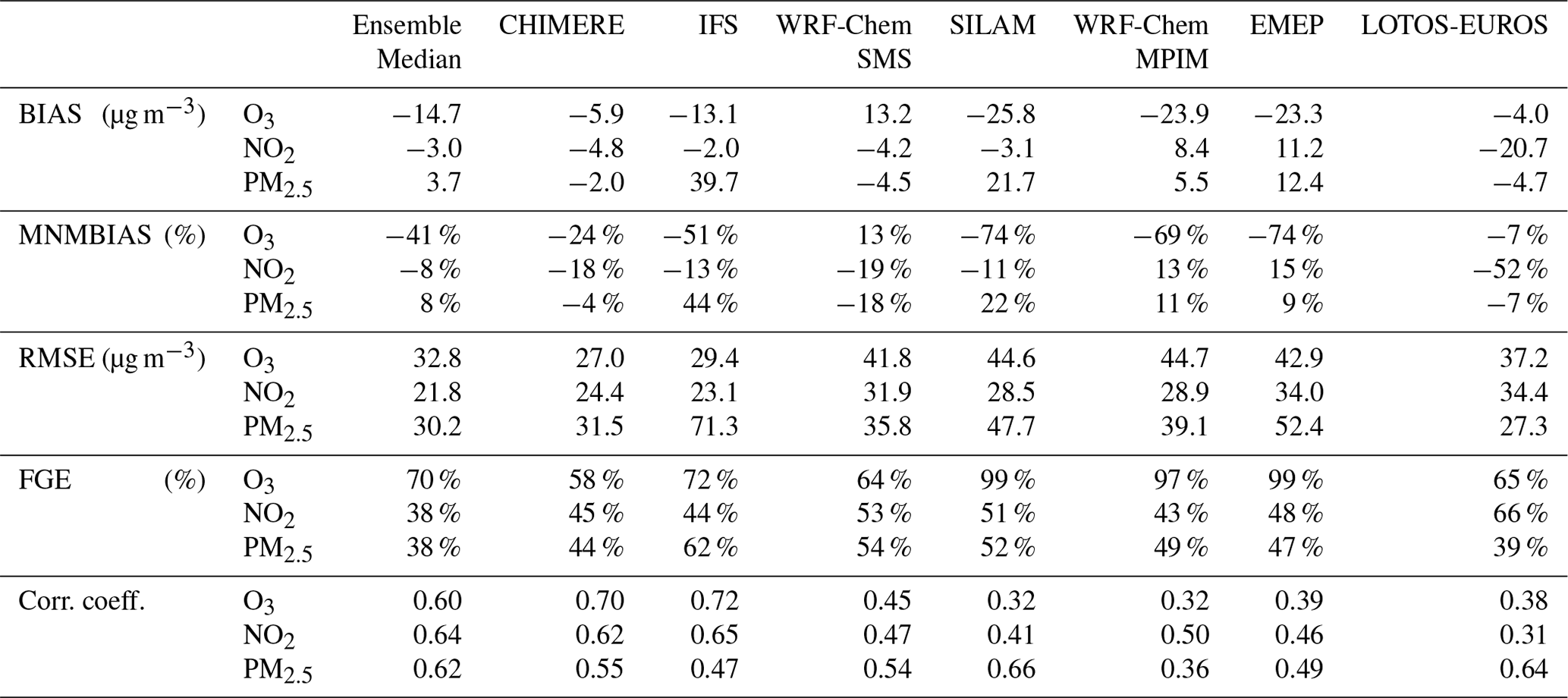
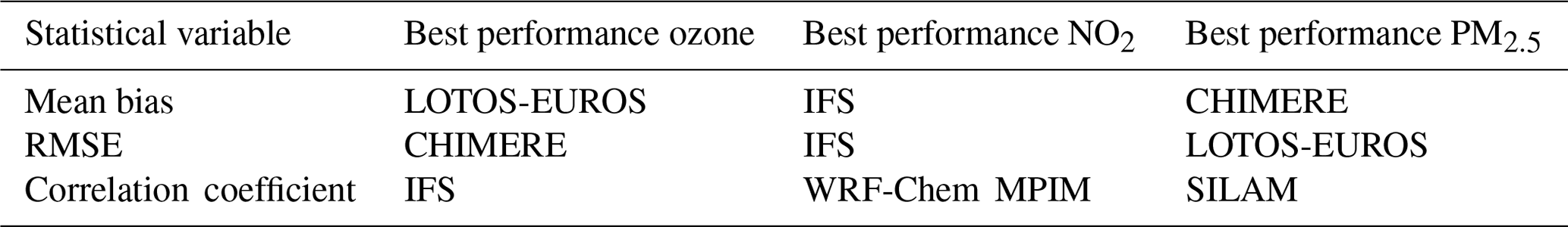
When examining the mean bias of the ensemble median, the values are equal to −14.7, −3.0, and +3.7 µg m−3 for ozone, NO2, and PM2.5, respectively, to be compared to mean concentration values of the order of 50 µg m−3 for these three different species. Table 4 shows that in the case of ozone, individual models are characterized by biases ranging from −25.8 (SILAM) to +13.2 µg m−3 (WRF-Chem-SMS), with the smallest absolute value equal to 5.9 µg m−3 (CHIMERE) The corresponding numbers range from −20.7 µg m−3 (LOTOS-EUROS) to +11.2 µg m−3 (EMEP) with the smallest absolute bias of −2.0 µg m−3 (IFS) for NO2. For PM2.5, they range from −4.7 µg m−3 (LOTOS-EUROS) to +39.6 µg m−3 (IFS) with the smallest absolute value equal to −2.0 µg m−3 (CHIMERE). In general, during the period chosen for the intercomparison, the models underestimate the ozone and NO2 concentrations and overestimate the concentration of PM2.5. The table also shows that the RMSE for the median values for ozone, NO2, and PM2.5 are 32.8, 21.8, and 30.2 µg m−3, respectively. With some exceptions (CHIMERE and IFS for ozone, LOTOS-EUROS, for PM2.5), these values are lower than the RMSE derived by individual models. The highest values for RMSE are 44.7 µg m−3 (WRF-Chem-MPIM) in the case of ozone, 34.4 (LOTOS EUROS) in the case of NO2, and 71.3 (IFS) in the case of PM2.5. The smallest RMSE are equal to 27.0 µg m−3 (CHIMERE) in the case of ozone, 23.1 µg m−3 (IFS) in the case of NO2, and 27.3 µg m−3 in the case of PM2.5 (LOTOS-EUROS). The correlation coefficient for the ensemble median is of the order of 0.6 for the three species, which in most cases is higher than the values derived from individual model forecasts. There are a few exceptions, however. The correlation coefficients are higher in the forecast of ozone by CHIMERE (0.70) and IFS (0.72), in the case of NO2 by IFS (0.65), and in the case of PM2.5 by SILAM (0.66) and LOTOS-EUROS (0.64). Table 5 summarizes the models that have achieved the best performance from the point of view of the mean bias, the RMSE, and the correlation coefficient.
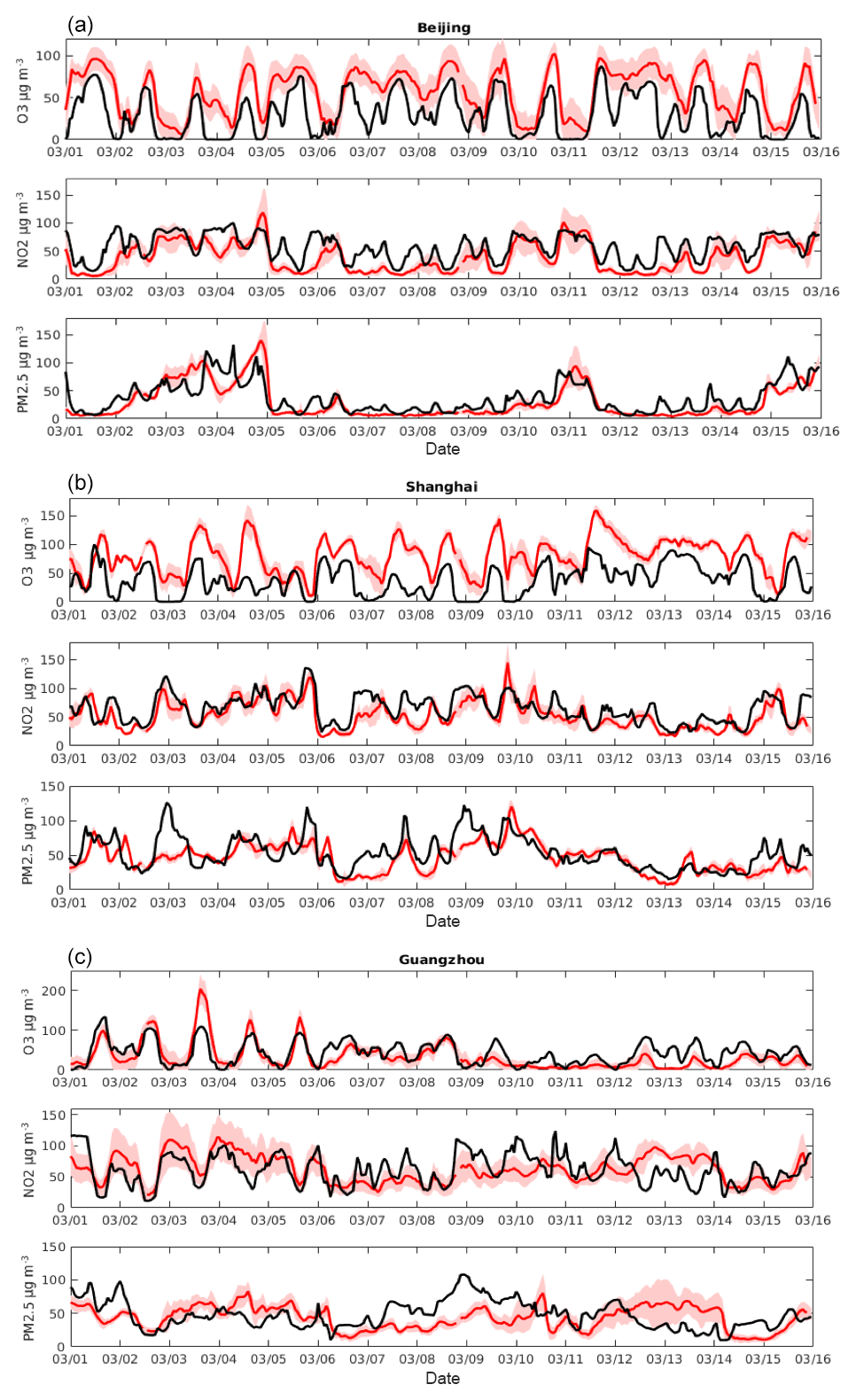
Figure 8Evolution of the surface concentrations of ozone, nitrogen dioxide, and particulate matter (diameter less than 2.5 µm) in (a) Beijing, (b) Shanghai, and (c) Guangzhou between 1 and 15 March 2017. In black: median of calculated values by the different models; in red: observed median concentrations.
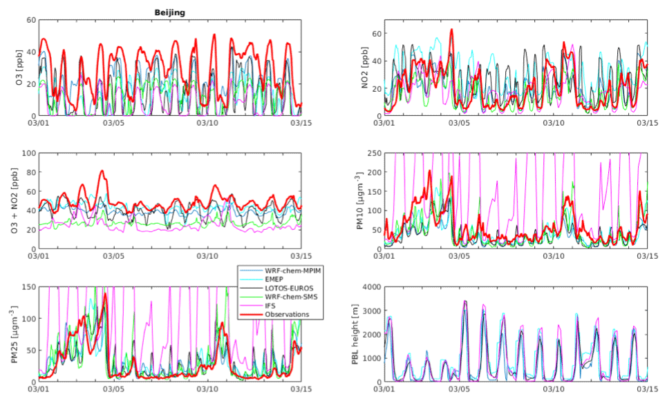
Figure 9Forecast of the chemical concentrations of ozone, NO2, PM2.5, and PM10 at Beijing between 1 and 15 March 2017 by the different models involved in the intercomparison conducted in the present study. The calculated values of as well as the height of the planetary boundary layer (PBL) are also shown. The mean values from the measurements made at the different monitoring stations of Beijing are shown by the thick red line.
5.4 Time evolution of individual forecasts
The time evolution of predicted concentration values at Beijing by five different models involved in the intercomparison is provided in Fig. 9 for the period of 1–15 March 2017. An examination of the figure shows that, during most days, the daytime height of the PBL reaches 2500–3000 m with an exception on 2 to 5 March, when the height does not exceed 1000 m. Interestingly, during this period, the observed concentration of particulates, of NO2, and of SO2, strongly influenced by surface emissions, are significantly higher than during the following days. During the same days, the nighttime concentration of ozone is relatively low. On 10 March, one also observes high surface concentrations of emitted species and a low concentration of nighttime ozone, even though the calculated PBL height is not particularly low. One should mention here that, in two models (i.e., EMEP and LOTOS-EUROS), the information on the PBL is deduced from the IFS forecast, while in other models (such as WRF-Chem-MPIM and WRF-Chem-SMS), the PBL height is derived independently. In the case of WRF-Chem-MPI, however, the calculation of the PBL height makes use of meteorological data provided by the IFS model.
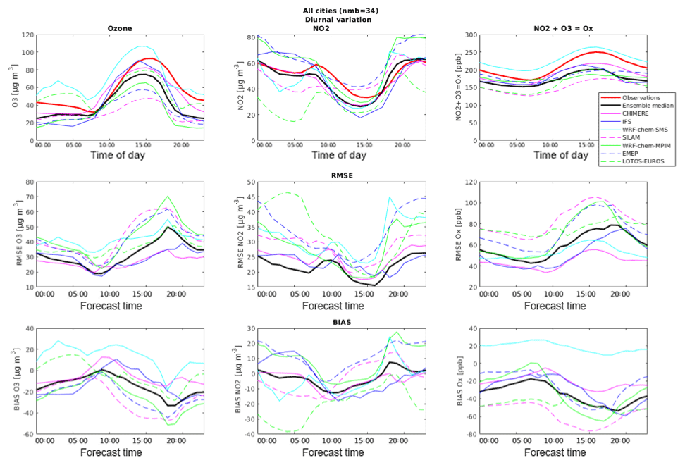
Figure 10Upper row: diurnal variation in ozone (left), NO2 (middle), and Ox = NO2 + O3 (right) for the period 1–15 March 2017 for all cities included in the MarcoPolo–Panda Prediction system for all seven models and the ensemble median and the observations (red line). Middle row: root mean square error (RMSE) for ozone (left), NO2 (middle), and Ox (right). Lower row: bias for ozone (left), NO2 (middle), and Ox (right) for all models and for the ensemble median (black line).
In most cases, the models capture the day-to-day variability in the species concentrations relatively well. The agreement with observations is generally good in the case of PM2.5 and PM10, except in the case of the IFS model, which considerably overestimates the concentrations, mainly because of a regional overestimation of the OM emissions and a lack of a diurnal variation in the emission. The anthropogenic OM emissions in IFS are parameterized based on anthropogenic CO emissions following Spracklen et al. (2011). The relatively high CO emission in this region may require a reduced conversion factor between OM and CO emissions. The main contribution to PM overestimation of IFS came from the nighttime values (see next section). Since nighttime overestimation also occurs for NO2, a lack of vertical mixing during the night in IFS could cause the nighttime overestimation of the surface values. As already noted, the models tend to underestimate the ozone concentrations, perhaps due to a slight overestimation of the nitrogen oxide concentrations. Another possible explanation is an underestimation of the VOC sources. Routine measurements of VOCs, however, are not available. The need for such measurements, however, needs to be stressed.
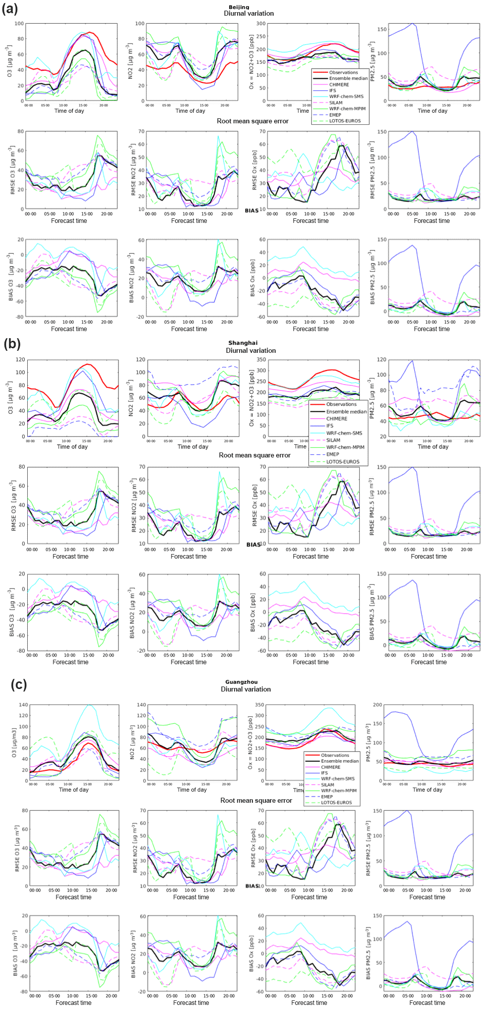
Figure 11(a) Same as Fig. 10 but for the urban area of Beijing. The statistical variables for PM2.5 are also included. (b) Same as Fig. 10 but for the urban area of Shanghai. The statistical variables for PM2.5 are also included. (c) Same as Fig. 10 but for the urban area of Guangzhou. The statistical variables for PM2.5 are also included.
The model comparison reported here also shows differences between models in the case of NO, which should probably be attributed to differences in the emissions and emission injection heights of this species and in the formulation of vertical mixing in the boundary layer. Here again, measurements of NO in addition to those of NO2 and ozone would be useful. Finally, one notes in Fig. 9 the relatively good agreement between models (with the exception of the IFS and the WRF-Chem-SMS model) regarding the time evolution of odd oxygen (). The models, however, slightly underestimate the absolute values of the Ox concentration.
5.5 Diurnal variations
In order to evaluate the behavior of the different models regarding their ability to reproduce the diurnal variation in the surface concentrations of ozone, NO2, and PM2.5, we have calculated the mean diurnal variations over the period of 1–15 March 2017 averaged for the 34 cities included in our analysis (3 of the 37 cities, located in the western part of the country and adopted in the MarcoPolo–Panda prediction system have not been considered in this analysis). The resulting results are shown in Fig. 10 for ozone and NO2 (expressed in µg m−3). We have added the corresponding diurnal evolution of Ox (expressed in ppbv) defined as the sum of the ozone and NO2 mixing ratios. This last chemical variable has the advantage that it is not affected by the fast interchange (null cycle) between ozone and NO2 by the reactions NO+O3, NO2 + hv, and O + O2 + M. Since this cycle tends to transfer “odd oxygen” from ozone to NO2 after sunset and from NO2 to ozone after sunrise, the Ox variable is less variable than its two components NO2 and O3 over a diurnal cycle. Figure 10 shows that, when averaging over the 34 largest Chinese cities, the diurnal variation in the ensemble median is in good agreement with the observation in the case of NO2. In the case of ozone, the median values are somewhat underestimated in late morning and in the afternoon. A similar situation is found in the case of Ox. The RMSE for ozone and NO2, also shown on the figure, is generally lower in the case of the ensemble median than for the individual models. In the case of PM2.5, however, the RMSE of the two models CHIMERE and IFS are smaller than the RMSE of the ensemble median (not shown here). The mean bias of the ensemble median for NO2 and ozone is generally smaller than that of the individual models. In the case of Ox, some models exhibit a positive bias (WRF-Chem SMS), while others (e.g., SILAM) are characterized by a negative bias.
Figure 11a, b, and c show similar estimates of the diurnal variation in the three large cities of China: Beijing, Shanghai, and Guangzhou. These graphs show that the ozone forecast from the ensemble median is lower than observed values during the entire day both in Beijing and in Shanghai. In Guangzhou, however, ozone is slightly overestimated by the prediction. In the case of NO2, the surface concentrations are overestimated in Beijing and to a lesser extent in Shanghai, with the largest overprediction occurring during nighttime, when the planetary boundary layer is very thin and vertical mixing almost shut off. At the same time, ozone is negatively biased due to its efficient titration by NOx. In the three cities, the RMSE of NO2, ozone, and Ox appear to be largest at sunset. Thus, a general issue with the MarcoPolo–Panda prediction system is the overestimation of surface NO2 and the underestimation of ozone concentrations during the nighttime.
In the case of PM2.5, one of the models involved (IFS) strongly overestimates the concentrations during nighttime but is in fair agreement with observations during daytime. This issue may again reflect a problem with the formulation of species dispersion in the planetary boundary layer. It may also be due to the lack of specified diurnal variation in the emission of primary pollutants as well as to the increased nighttime stability.
The intercomparison presented in the previous sections provides useful information and represents the basis on which the accuracy of the model predictions can be improved. Since the models have been developed fairly independently and the choices about input parameters such as emissions, chemical schemes, and adopted weather forecasts have been based on best judgement by these individual teams, a statistical treatment of the model results (e.g., determination of averages and standard deviation) provides, in general, more reliable information than the data provided by the individual model components of the ensemble. The examination of the model output reveals, however, some systematic biases that could be reduced by identifying the likely cause of these errors.
A simple approach is to recognize that the failure of models to correctly predict air quality could result from several factors: (1) errors in the adopted emissions and the formulation of boundary layer dispersion best diagnosed by analyzing the ability of the model to reproduce the monthly mean surface concentrations of chemical species; (2) errors or omission in the adopted chemical scheme leading to inaccuracies in the calculated mean diurnal variations in the concentrations of secondary species; and (3) inaccuracies in the adopted weather forecasts leading to poorly calculated day-to-day variations in the calculated chemical fields. In this later case, one should distinguish between fundamental model biases (i.e., the representation of PBL mixing, a bias that is intrinsic to the models) and the increasing error in the forecast of synoptic weather patterns as the model integration proceeds. This probably provides an oversimplified view of the causes of errors in chemical weather forecasts, but it offers a simple approach to address some issues in the models and hence to improve the predictions.
A first step towards the improvement of the different model components will be to conduct additional simulations by adopting the same best available emissions data and the same meteorological forecasts. Remaining differences between the models will be due in large part (although not exclusively) to the adopted chemical scheme and the formulation of boundary layer processes. An additional step would be to bring the different formulations of chemistry closer together by at least harmonizing the adopted rate constants and using the same module to calculate photodissociation rates. Finally, it would be interesting to assess the differences in chemical weather predictions resulting from the adopted meteorological forecasts. In particular, it would be important to better constrain the differences in the photolysis rates resulting from the adopted or calculated concentrations of aerosols and in cloudiness. One single model could be run for several days with the weather predictions produced by different meteorological centers.
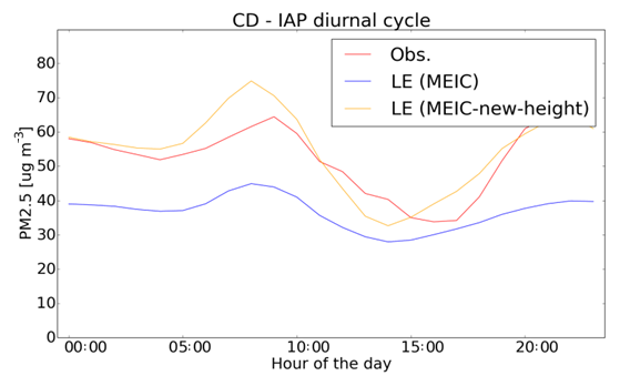
Figure 12Annually averaged diurnal evolution of the PM2.5 concentrations in the city of Chengdu simulated for different values of the particulate injection height. Calculations by the LOTOS-EUROS (LE) model.
Finally, a few specific issues from the present intercomparison require attention:
-
Most models overestimate the surface levels of NO2 and PM2.5 as well as other species emitted at the surface, specifically during nighttime. The largest discrepancies appear around 18:00 LT when the surface cools and the boundary layer collapses and the emitted species remain trapped in the lowest model layers. Evidently, these models underestimate the vertical exchanges between layers probably produced by the turbulence thermally or mechanically generated by the presence of buildings. Such effects are not accounted for in models that do include a specialized urban formulation. The overestimation of NO2 during nighttime leads to the titration of ozone near the surface and hence an underestimation of the concentration of this gas. The emission injection height is also a relevant factor here, which can largely influence results. During nighttime, emissions from stacks may be emitted above the mixing layer. However, if the injection height in the model is put at a lower altitude (or even at the surface), this could lead to an overestimation of emissions. The LOTOS-EUROS model evaluated the impact of emission injection heights. An update of the emission heights was tested that injects emissions from industry at lower heights, indicating that the number of high stacks is limited (and not that, contrary to most models, the concentrations at nighttime are often underestimated in the case of LOTOS-EUROS; see Figs. 10 and 11). Figure 12 shows diurnal cycles of the simulated PM2.5 concentrations in the city of Chengdu, averaged over an entire year. The updated emission heights clearly have a large (positive) impact on the simulations.
-
Daytime concentrations of ozone are generally underestimated in most regions of eastern China, even when the level of NO2 is in reasonable agreement with the values reported by the monitoring stations. The discrepancy could be caused by an underestimation of the emissions of some VOCs, especially in urban areas where ozone is often VOC-limited. More work is required to investigate this question.
-
Emissions of primary pollutants are changing extremely rapidly in China. The adopted emissions inventories usually reflect the situation a few years before the present day. Since the current emissions have decreased significantly in some urban areas of China in response to measures taken by the authorities, the emissions used in this case for current forecasts may be overestimated. For example, the EMEP model team applied a reduction in NOx emissions after the study period of March 2017 and thereby, through less ozone titration, reduced the severe underestimation of ozone.
-
Land-use data. Due to the rapid development occurring in particular in the eastern part of China, land-use data and vegetation change rapidly, and datasets in the model may not accurately reflect the current situation. This has an influence on emissions (including biogenic) but also on the deposition of pollutants and even meteorology. Land-use data should be updated using satellite observations, urban planning maps, and other data sources.
An operational multi-model air quality forecast system has been established through a close cooperation between European and Chinese research groups and with the support of the European Commission (7th Framework Programme). This system provides daily forecasts for the surface concentration of key pollutants in eastern China and particularly in the major urban centers of the country. These predictions are posted on a dedicated website (http://www.marcopolo-panda.eu/, last access: 7 December 2018), where they are compared hour by hour to surface measurements for each city, performed at the monitoring stations deployed in China by the PM2.5 network (http://pm25.in/).
The discussions presented in this paper show that in most cases, the model ensemble reproduces quite satisfactorily the synoptic behavior and the day-to-day variability of the concentrations of ozone and particulate matter and, in particular, predicts the development of most air pollution episodes a few days before their occurrence. This must be attributed to the quality of the weather forecasts at the synoptic scales that are used for the calculation of chemical species. Overall and in spite of some discrepancies that have been highlighted in the previous sections, the forecast system can therefore be regarded as successful.
The system is in its early phase of development and the purpose of the intercomparison exercise presented here was to diagnose differences between models and perhaps identify errors. An important objective was to determine ways by which the models could be improved. Even though, in many instances, the surface concentrations are in good or fair agreement with the measured values, differences between calculated and observed values can occasionally be substantial. These occasional differences are often attributed to inaccuracies in the weather forecasts for specific days, but errors in the adopted surface emissions and PBL exchanges or the simplifications introduced in the adopted chemical and aerosol schemes can also be substantial.
The degree by which the concentrations derived by global and regional models, even at high spatial resolution, can be compared with local measurements made in a complex urban canopy remains an important issue that requires further investigation. The insertion of more detailed land-use modules or of a large eddy simulation system in the chemical transport models should be considered in future studies.
The models described here are used operationally by the participating research and service organizations involved in the present study. The data produced by the multi-model forecasting system are available from the KNMI.
| AC-SAF | Atmospheric Composition–Satellite Application Facilities |
| ADAS | the ARPS (the Advanced Regional Prediction System) Data Assimilation System |
| AERO5 | the fifth-generation modal CMAQ aerosol model |
| AOD | aerosol optical depth |
| BIAS | mean bias |
| CAMS | Copernicus Atmospheric Monitoring Service |
| CBM | carbon bond mechanism |
| CMAQ | United States Environmental Prediction Agency, Community Multiscale Air Quality Model |
| CNES | National Centre for Space Studies |
| CO | carbon monoxide |
| COPD | chronic obstructive pulmonary disease |
| DMAT | Dispersion Model for Atmospheric Transport |
| ECMWF | European Centre for Medium-Range Weather Forecasts |
| EDGAR | Emission Database for Global Atmospheric Research |
| EMEP | European Monitoring and Evaluation Programme |
| EOS | the Earth Observing System |
| ESA | European Space Agency |
| EUMETSAT | The European Organisation for the Exploitation of Meteorological Satellites |
| FGE | fractional gross error |
| FMI | Finnish Meteorological Institute |
| FNL | Final Operational Global Analysis data |
| FP7 | Framework Programme 7 |
| FRP | fire radiative power |
| GFAS | Global Fire Assimilation System |
| GFS | Global Forecast System |
| GO-CART | The Goddard Chemistry Aerosol Radiation and Transport model |
| GOME | The Global Ozone Monitoring Experiment |
| HTAP | Hemispheric Transport of Air Pollution |
| IASI | Infrared Atmospheric Sounding Interferometer |
| IFS | Integrated Forecasting System |
| ISORROPIA | an aerosol thermodynamic model |
| KNMI | Royal Netherlands Meteorological Institute |
| LAI | leaf area index |
| LATMOS | Laboratoire Atmosphères Milieux Observations Spatiales |
| LMDz- INCA | Laboratoire de Météorologie Dynamique, version 4 – INteraction with Chemistry and Aerosols, version 3 |
| LOTOS-EUROS | Long-term Ozone Simulations – European Operational Smog model |
| MACCity | an anthropogenic emission inventory derived from the ACCMIP and RCP8.5 datasets as part of two projects funded by the European Commission: MACC (Monitoring Atmospheric Composition and Climate) and CityZEN. (http://eccad.aeris-data.fr/, last access: 14 December 2018) |
| MARS | Model for the Atmospheric Dispersion of Reactive Species |
| MEGAN | Model of Emissions of Gases and Aerosols from Nature |
| MEIC | Multi-resolution Emission Inventory for China |
| MET.Norway | Norwegian Meteorological Institute |
| MIX | a mosaic Asian anthropogenic emission inventory under the international collaboration framework of the MICS-Asia (Model Inter-Comparison Study for Asia) and HTAP. (http://www.meicmodel.org/dataset-mix, last access: 14 December 2018) |
| MLS | Microwave Limb Sounder |
| MNMBIAS | mean normalized bias |
| MODIS | Moderate Resolution Imaging Spectroradiometer |
| MOPITT | Measurements Of Pollution In The Troposphere |
| MOSAIC | the Model for Simulating Aerosol Interactions and Chemistry |
| MOZART | the Model for Ozone and Related Chemical Tracers |
| MPIM | Max Planck Institute for Meteorology |
| MSC-W | Meteorological Synthesizing Centre – West Model |
| NASA | National Aeronautics and Space Administration |
| NCAR | National Center for Atmospheric Research |
| NCEP | National Centers for Environmental Prediction |
| NCP | North China Plain |
| NJU | Nanjing University |
| NMVOC | non-methane volatile organic compound |
| NOAA | National Oceanic and Atmospheric Administration |
| NO2 | nitrogen dioxide |
| NOx | nitrogen oxides |
| O3 | ozone |
| OM | organic matter |
| OMI | Ozone Monitoring Instrument |
| OMPS | the Ozone Mapping And Profiler Suite |
| PBL | planetary boundary layer |
| PM | particulate matter |
| PMAp | Polar Multi-Sensor Aerosol product |
| RADM2 | Regional Acid Deposition Model version 2 |
| RMSE | root mean square error |
| SBUV | Solar Backscatter Ultraviolet instrument |
| SCUEM | Shanghai Centre on Urban Environmental Meteorology |
| SILAM | System for Integrated Modeling of Atmospheric Composition |
| SMS | Shanghai Meteorological Service |
| SO2 | sulfur dioxide |
| SOA | secondary organic aerosol |
| SORGAM | Secondary ORGanic Aerosol Model |
| STEAM | the Ship Traffic Emission Assessment Model |
| Suomi-NPP | Suomi National Polar-orbiting Partnership |
| TNO | the Netherlands Organisation for Applied Scientific Research |
| TUV | Tropospheric Ultraviolet-Visible model |
| U.S. EPA | US Environmental Protection Agency |
| ULB | Université Libre de Bruxelles |
| VBS | volatility basis set |
| VOC | volatile organic compounds |
| WRF-Chem | Weather Research and Forecasting model coupled to chemistry |
| YSU | Yonsei University |
GPB coordinated the Panda Project and contributed to the analysis of the results provided by the WRF-Chem model. RvdA coordinated the MarcoPolo Project and was involved in the analysis of the results provided by the Chimere model. AKP, IB and SW were in charge of the WRF-Chem simulations. YX, JX and GZ developed and used the WRF-Chem-SMS model. VHP and JF performed the simulations with the IFS model. MG and MP were in charge of the simulations performed by the EMEP model. FJ is in charge of the WRF-CMAQ model. MS and RK were responsible for the forecasts made the SILAM model, while RT, AS and RK were using the LOTOS-EUROS model. BM developed the MarcoPolo and Panda website and collected all the model results and observational data.
The authors declare that they have no conflict of interest.
The model intercomparison presented in the present study was conducted
during a workshop organized in May 2017 by the Shanghai Meteorological
Service (SMS) in China. The authors thank Jianming Xu for hosting this
meeting and providing support to the participants. The ensemble of models
described here has been produced under the Panda and MarcoPolo projects
supported by the European Commission within the Framework Program 7 (FP7)
under grant agreements no. 606719 and no. 606953. The
National Center for Atmospheric Research (NCAR) is sponsored by the US
National Science Foundation.
The article processing charges for this open-access
publication were covered by the Max Planck Society.
Edited by: David Topping
Reviewed by: two anonymous referees
Appel, K. W., Napelenok, S. L., Foley, K. M., Pye, H. O. T., Hogrefe, C., Luecken, D. J., Bash, J. O., Roselle, S. J., Pleim, J. E., Foroutan, H., Hutzell, W. T., Pouliot, G. A., Sarwar, G., Fahey, K. M., Gantt, B., Gilliam, R. C., Heath, N. K., Kang, D., Mathur, R., Schwede, D. B., Spero, T. L., Wong, D. C., and Young, J. O.: Description and evaluation of the Community Multiscale Air Quality (CMAQ) modeling system version 5.1, Geosci. Model Dev., 10, 1703–1732, https://doi.org/10.5194/gmd-10-1703-2017, 2017.
Bauer, P., Thorpe A., and Brunet G.: The quiet revolution of numerical weather prediction, Nature, 525, 47–55, 2015.
Bergström, R., Denier van der Gon, H. A. C., Prévôt, A. S. H., Yttri, K. E., and Simpson, D.: Modelling of organic aerosols over Europe (2002–2007) using a volatility basis set (VBS) framework: application of different assumptions regarding the formation of secondary organic aerosol, Atmos. Chem. Phys., 12, 8499–8527, https://doi.org/10.5194/acp-12-8499-2012, 2012.
Byun, D. and Schere, K. L.: Review of the governing equations, computational algorithms, and other components of the Models-3 Community Multiscale Air Quality (CMAQ) modeling system, Appl. Mech. Rev., 59, 51–77, 2006.
Carlton, A. G., Bhave, P. V., Napelenok, S. L., Edney, E. O., Sarwar, G., Pinder, R. W., Pouliot, G. A., and Houyoux, M.: Model Representation of Secondary Organic Aerosol in CMAQv4.7, Environ. Sci. Technol., 44, 8553–8560, 2010.
Chang, J. S., Binkowski, F. S., Seaman, N. L., McHenry, J. N., Samson, P. J., Stockwell, W. R., Walcek, C. J., Madronich, S., Middleton, P. B., Pleim, J. E., and Lansford, H. H.: The regional acid deposition model and engineering model, State-of-Science/Technology, Report 4, National Acid Precipitation Assessment Program, Washington, DC, 1989.
Crippa, M., Janssens-Maenhout, G., Dentener, F., Guizzardi, D., Sindelarova, K., Muntean, M., Van Dingenen, R., and Granier, C.: Forty years of improvements in European air quality: regional policy-industry interactions with global impacts, Atmos. Chem. Phys., 16, 3825–3841, https://doi.org/10.5194/acp-16-3825-2016, 2016.
Dabberdt, W. F. and Miller, E.: Uncertainty, ensembles and air quality dispersion modeling: applications and challenges, Atmos. Environ., 34, 4667-4673, 2000.
Donahue, N. M., Robinson, A. L., Stanier, C. O., and Pandis, S. N.: Coupled partitioning, dilution, and chemical aging of semivolatile organics, Environ. Sci. Technol., 40, 2635–2643, https://doi.org/10.1021/Es052297c, 2006.
Emmons, L. K., Walters, S., Hess, P. G., Lamarque, J.-F., Pfister, G. G., Fillmore, D., Granier, C., Guenther, A., Kinnison, D., Laepple, T., Orlando, J., Tie, X., Tyndall, G., Wiedinmyer, C., Baughcum, S. L., and Kloster, S.: Description and evaluation of the Model for Ozone and Related chemical Tracers, version 4 (MOZART-4), Geosci. Model Dev., 3, 43–67, https://doi.org/10.5194/gmd-3-43-2010, 2010.
Fast, J. D., Gustafson, W. I., Easter, R. C., Zaveri, R. A., Barnard, J. C., Chapman, E. G., Grell, G. A. and Peckham, S. E.: Evolution of ozone, particulates, and aerosol direct radiative forcing in the vicinity of Houston using a fully coupled meteorology-chemistry-aerosol model, J. Geophys. Res., 111, D21305, https://doi.org/10.1029/2005JD006721, 2006.
Flemming, J., Huijnen, V., Arteta, J., Bechtold, P., Beljaars, A., Blechschmidt, A.-M., Diamantakis, M., Engelen, R. J., Gaudel, A., Inness, A., Jones, L., Josse, B., Katragkou, E., Marecal, V., Peuch, V.-H., Richter, A., Schultz, M. G., Stein, O., and Tsikerdekis, A.: Tropospheric chemistry in the Integrated Forecasting System of ECMWF, Geosci. Model Dev., 8, 975–1003, https://doi.org/10.5194/gmd-8-975-2015, 2015.
Foley, K. M., Roselle, S. J., Appel, K. W., Bhave, P. V., Pleim, J. E., Otte, T. L., Mathur, R., Sarwar, G., Young, J. O., Gilliam, R. C., Nolte, C. G., Kelly, J. T., Gilliland, A. B., and Bash, J. O.: Incremental testing of the Community Multiscale Air Quality (CMAQ) modeling system version 4.7, Geosci. Model Dev., 3, 205–226, https://doi.org/10.5194/gmd-3-205-2010, 2010.
Fountoukis, C. and Nenes, A.: ISORROPIA II: a computationally efficient thermodynamic equilibrium model for K+–Ca2+–Mg2+––Na+–––Cl−–H2O aerosols, Atmos. Chem. Phys., 7, 4639–4659, https://doi.org/10.5194/acp-7-4639-2007, 2007.
Galmarini, S., Kioutsioukis, I., and Solazzo, E.: E pluribus unum*: ensemble air quality predictions, Atmos. Chem. Phys., 13, 7153–7182, https://doi.org/10.5194/acp-13-7153-2013, 2013.
Ginoux, P., Chin, M., Tegen, I., Prospero, J. M., Holben, B., Dubovik, O., and Lin, S.-J.: Sources and distributions of dust aerosols simulated with the GOCART model, J. Geophys. Res., 106, 20255–20273, 2001.
Granier, C, Bessagnet, B., Bond, T., D'Angiola, A., Denier van der Gon, H., Frost, G. J., Heil, A., Kaiser, J. W., Kinne, S., Klimont, Z., Kloster, S., Lamarque, J.-F., Liousse, C., Masui, T., Meleux, F., Mieville, A., Ohara, T., Raut, J.-C., Riahi, K., Schultz, M. G., Smith, S. J., Thompson, A., van Aardenne, J., van der Werf, G. R., and van Vuuren, D. P.:, Evolution of anthropogenic and biomass burning emissions at global and regional scales during the 1980–2010 period, Climatic Change, 109, 163, https://doi.org/10.1007/s10584-011-0154-1, 2011.
Grell, G. A., Peckham, S. E., Schmitz, R., McKeen, S. A., Frost, G., Skamarock, W. C., and Eder, B.: Fully coupled “online” chemistry in the WRF model. Atmos. Environ., 39, 6957–6976, 2005.
Guenther, A., Karl, T., Harley, P., Wiedinmyer, C., Palmer, P. I., and Geron, C.: Estimates of global terrestrial isoprene emissions using MEGAN (Model of Emissions of Gases and Aerosols from Nature), Atmos. Chem. Phys., 6, 3181–3210, https://doi.org/10.5194/acp-6-3181-2006, 2006.
Guenther, A. B., Jiang, X., Heald, C. L., Sakulyanontvittaya, T., Duhl, T., Emmons, L. K., and Wang, X.: The Model of Emissions of Gases and Aerosols from Nature version 2.1 (MEGAN2.1): an extended and updated framework for modeling biogenic emissions, Geosci. Model Dev., 5, 1471–1492, https://doi.org/10.5194/gmd-5-1471-2012, 2012.
Hodzic, A. and Jimenez, J. L.: Modeling anthropogenically controlled secondary organic aerosols in a megacity: a simplified framework for global and climate models, Geosci. Model Dev., 4, 901–917, https://doi.org/10.5194/gmd-4-901-2011, 2011.
Hu, J., Chen, J., Ying, Q., and Zhang, H.: One-year simulation of ozone and particulate matter in China using WRF/CMAQ modeling system, Atmos. Chem. Phys., 16, 10333–10350, https://doi.org/10.5194/acp-16-10333-2016, 2016.
Huijnen, V., Williams, J., van Weele, M., van Noije, T., Krol, M., Dentener, F., Segers, A., Houweling, S., Peters, W., de Laat, J., Boersma, F., Bergamaschi, P., van Velthoven, P., Le Sager, P., Eskes, H., Alkemade, F., Scheele, R., Nédélec, P., and Pätz, H.-W.: The global chemistry transport model TM5: description and evaluation of the tropospheric chemistry version 3.0, Geosci. Model Dev., 3, 445–473, https://doi.org/10.5194/gmd-3-445-2010, 2010.
Inness, A., Blechschmidt, A.-M., Bouarar, I., Chabrillat, S., Crepulja, M., Engelen, R. J., Eskes, H., Flemming, J., Gaudel, A., Hendrick, F., Huijnen, V., Jones, L., Kapsomenakis, J., Katragkou, E., Keppens, A., Langerock, B., de Mazière, M., Melas, D., Parrington, M., Peuch, V. H., Razinger, M., Richter, A., Schultz, M. G., Suttie, M., Thouret, V., Vrekoussis, M., Wagner, A., and Zerefos, C.: Data assimilation of satellite-retrieved ozone, carbon monoxide and nitrogen dioxide with ECMWF's Composition-IFS, Atmos. Chem. Phys., 15, 5275–5303, https://doi.org/10.5194/acp-15-5275-2015, 2015.
Janssens-Maenhout, G., Crippa, M., Guizzardi, D., Dentener, F., Muntean, M., Pouliot, G., Keating, T., Zhang, Q., Kurokawa, J., Wankmüller, R., Denier van der Gon, H., Kuenen, J. J. P., Klimont, Z., Frost, G., Darras, S., Koffi, B., and Li, M.: HTAP_v2.2: a mosaic of regional and global emission grid maps for 2008 and 2010 to study hemispheric transport of air pollution, Atmos. Chem. Phys., 15, 11411–11432, https://doi.org/10.5194/acp-15-11411-2015, 2015.
Jonson, J. E., Stohl, A., Fiore, A. M., Hess, P., Szopa, S., Wild, O., Zeng, G., Dentener, F. J., Lupu, A., Schultz, M. G., Duncan, B. N., Sudo, K., Wind, P., Schulz, M., Marmer, E., Cuvelier, C., Keating, T., Zuber, A., Valdebenito, A., Dorokhov, V., De Backer, H., Davies, J., Chen, G. H., Johnson, B., Tarasick, D. W., Stübi, R., Newchurch, M. J., von der Gathen, P., Steinbrecht, W., and Claude, H.: A multi-model analysis of vertical ozone profiles, Atmos. Chem. Phys., 10, 5759–5783, https://doi.org/10.5194/acp-10-5759-2010, 2010.
Kaiser, J. W., Heil, A., Andreae, M. O., Benedetti, A., Chubarova, N., Jones, L., Morcrette, J.-J., Razinger, M., Schultz, M. G., Suttie, M., and van der Werf, G. R.: Biomass burning emissions estimated with a global fire assimilation system based on observed fire radiative power, Biogeosciences, 9, 527–554, https://doi.org/10.5194/bg-9-527-2012, 2012.
Kouznetsov, R. and Sofiev, M.: A methodology for evaluation of vertical dispersion and dry deposition of atmospheric aerosols, J. Geophys. Res., 117, D01202, https://doi.org/10.1029/2011JD016366, 2012.
Kukkonen, J., Olsson, T., Schultz, D. M., Baklanov, A., Klein, T., Miranda, A. I., Monteiro, A., Hirtl, M., Tarvainen, V., Boy, M., Peuch, V.-H., Poupkou, A., Kioutsioukis, I., Finardi, S., Sofiev, M., Sokhi, R., Lehtinen, K. E. J., Karatzas, K., San José, R., Astitha, M., Kallos, G., Schaap, M., Reimer, E., Jakobs, H., and Eben, K.: A review of operational, regional-scale, chemical weather forecasting models in Europe, Atmos. Chem. Phys., 12, 1–87, https://doi.org/10.5194/acp-12-1-2012, 2012.
Li, M., Zhang, Q., Streets, D. G., He, K. B., Cheng, Y. F., Emmons, L. K., Huo, H., Kang, S. C., Lu, Z., Shao, M., Su, H., Yu, X., and Zhang, Y.: Mapping Asian anthropogenic emissions of non-methane volatile organic compounds to multiple chemical mechanisms, Atmos. Chem. Phys., 14, 5617–5638, https://doi.org/10.5194/acp-14-5617-2014, 2014.
Li, M., Zhang, Q., Kurokawa, J.-I., Woo, J.-H., He, K., Lu, Z., Ohara, T., Song, Y., Streets, D. G., Carmichael, G. R., Cheng, Y., Hong, C., Huo, H., Jiang, X., Kang, S., Liu, F., Su, H., and Zheng, B.: MIX: a mosaic Asian anthropogenic emission inventory under the international collaboration framework of the MICS-Asia and HTAP, Atmos. Chem. Phys., 17, 935–963, https://doi.org/10.5194/acp-17-935-2017, 2017.
Liu, F., Zhang, Q., Tong, D., Zheng, B., Li, M., Huo, H., and He, K. B.: High-resolution inventory of technologies, activities, and emissions of coal-fired power plants in China from 1990 to 2010, Atmos. Chem. Phys., 15, 13299–13317, https://doi.org/10.5194/acp-15-13299-2015, 2015.
Lorenc, A. C: A global three-dimensional multivariate statistical interpolation scheme, Mon. Weather Rev., 109, 701–721, 1981.
Madronich, S. and Flocke, S.: The role of solar radiation in atmospheric chemistry, edited by: Boule, P., Handbook of Environmental Chemistry, Springer, Heidelberg, 1999.
Manders, A. M. M., Builtjes, P. J. H., Curier, L., Denier van der Gon, H. A. C., Hendriks, C., Jonkers, S., Kranenburg, R., Kuenen, J. J. P., Segers, A. J., Timmermans, R. M. A., Visschedijk, A. J. H., Wichink Kruit, R. J., van Pul, W. A. J., Sauter, F. J., van der Swaluw, E., Swart, D. P. J., Douros, J., Eskes, H., van Meijgaard, E., van Ulft, B., van Velthoven, P., Banzhaf, S., Mues, A. C., Stern, R., Fu, G., Lu, S., Heemink, A., van Velzen, N., and Schaap, M.: Curriculum vitae of the LOTOS–EUROS (v2.0) chemistry transport model, Geosci. Model Dev., 10, 4145–4173, https://doi.org/10.5194/gmd-10-4145-2017, 2017.
Marécal, V., Peuch, V.-H., Andersson, C., Andersson, S., Arteta, J., Beekmann, M., Benedictow, A., Bergström, R., Bessagnet, B., Cansado, A., Chéroux, F., Colette, A., Coman, A., Curier, R. L., Denier van der Gon, H. A. C., Drouin, A., Elbern, H., Emili, E., Engelen, R. J., Eskes, H. J., Foret, G., Friese, E., Gauss, M., Giannaros, C., Guth, J., Joly, M., Jaumouillé, E., Josse, B., Kadygrov, N., Kaiser, J. W., Krajsek, K., Kuenen, J., Kumar, U., Liora, N., Lopez, E., Malherbe, L., Martinez, I., Melas, D., Meleux, F., Menut, L., Moinat, P., Morales, T., Parmentier, J., Piacentini, A., Plu, M., Poupkou, A., Queguiner, S., Robertson, L., Rouïl, L., Schaap, M., Segers, A., Sofiev, M., Tarasson, L., Thomas, M., Timmermans, R., Valdebenito, Á., van Velthoven, P., van Versendaal, R., Vira, J., and Ung, A.: A regional air quality forecasting system over Europe: the MACC-II daily ensemble production, Geosci. Model Dev., 8, 2777–2813, https://doi.org/10.5194/gmd-8-2777-2015, 2015.
McKeen, S., Wilczak, J., Grell, G., Djalalova, I., Peckham, S., Hsie, E.-Y., Gong, W., Bouchet, V., Menard, S., Moffet, R., McHenry, J., McQueen, J., Tang, Y., Carmichael, G. R., Pagowski, M., Chan, A., Dye, T., Frost, G., Lee, P., and Mathur R., Assessment of an ensemble of seven real-time ozone forecasts over Eastern North America during the summer of 2004, J. Geophys. Res., 110, D21307, https://doi.org/10.1029/2005JD005858, 2005.
Menut, L., Bessagnet, B., Khvorostyanov, D., Beekmann, M., Blond, N., Colette, A., Coll, I., Curci, G., Foret, G., Hodzic, A., Mailler, S., Meleux, F., Monge, J.-L., Pison, I., Siour, G., Turquety, S., Valari, M., Vautard, R., and Vivanco, M. G.: CHIMERE 2013: a model for regional atmospheric composition modelling, Geosci. Model Dev., 6, 981–1028, https://doi.org/10.5194/gmd-6-981-2013, 2013a.
Menut, L., Perez Garcia-Pando, C., Haustein, K., Bessagnet, B., Prigent, C., and Alfaro, S.: Relative impact of roughness and soil texture on mineral dust emission fluxes modeling, J. Geophys. Res., 118, 6505–6520, https://doi.org/10.1002/jgrd.50313, 2013b.
Monahan, E. C., Spiel, D. E., and Davidson, K. L.: A Model of Marine Aerosol Generation Via Whitecaps and Wave Disruption, in: Oceanic Whitecaps, Oceanographic Sciences Library, edited by: Monahan, E. C. and Niocaill, G. M., vol 2., Springer, Dordrecht, 1986.
Morcrette, J.-J., Boucher, O., Jones, L., Salmond, D., Bechtold, P., Beljaars, A., Benedetti, A., Bonet, A., Kaiser, J. W., Razinger, M., Schulz, M., Serrar, S., Simmons, A. J., Sofiev, M., Suttie, M., Tompkins, A. M., and Untch, A.: Aerosol analysis and forecast in the ECMWF Integrated Forecast System. Part I: Forward modelling, J. Geophys. Res., D06206, https://doi.org/10.1029/2008JD011235, 2009.
Muntean, M., Janssens-Maenhout, G., Song, S., Selin, N. E., Olivier, J. G. J., Guizzardi, D., Maas, R., and Dentener, F., Trend analysis from 1970 to 2008 and model evaluation of EDGARv4 global gridded anthropogenic mercury emissions, Sci. Total Environ., 494–495, 337–350, 2014.
Petersen, A. K., Brasseur, G. P., Bouarar, I., Flemming, J., Gauss, M., Jiang, F., Kouznetsov, R., Kranenburg, R., Mijling, B., Peuch, V.-H., Pommier, M., Segers, A., Sofiev, M., Timmermans, R., van der A, R., Walters, S., Xie, Y., Xu, J., and Zhou, G.: Ensemble Forecasts of Air Quality in Eastern China – Part 2. Evaluation of the MarcoPolo-Panda Prediction System, Version 1, Geosci. Model Dev. Discuss., https://doi.org/10.5194/gmd-2018-234, in review, 2018.
Poupkou, A., Giannaros, T., Markakis, K., Kioutsioukis, I., Curci, G., Melas, D., and Zerefos, C.: A model for European Biogenic Volatile Organic Compound emissions: Software development and first validation, Environ. Modell. Softw., 25, 1845–1856, 2010.
Riccio, A., Giunta, G., and Galmarini, S.: Seeking for the rational basis of the Median Model: the optimal combination of multi-model ensemble results, Atmos. Chem. Phys., 7, 6085–6098, https://doi.org/10.5194/acp-7-6085-2007, 2007.
Schell, B., Ackermann, I. J., Hass, H., Binkowski, F. S., and Ebel, A.: Modeling the formation of secondary organic aerosol within a comprehensive air quality model system, J. Geophys. Res., 106, 28275–28293, 2001.
Shrivastava, M., Fast, J., Easter, R., Gustafson Jr., W. I., Zaveri, R. A., Jimenez, J. L., Saide, P., and Hodzic, A.: Modeling organic aerosols in a megacity: comparison of simple and complex representations of the volatility basis set approach, Atmos. Chem. Phys., 11, 6639–6662, https://doi.org/10.5194/acp-11-6639-2011, 2011.
Simpson, D., Benedictow, A., Berge, H., Bergström, R., Emberson, L. D., Fagerli, H., Flechard, C. R., Hayman, G. D., Gauss, M., Jonson, J. E., Jenkin, M. E., Nyíri, A., Richter, C., Semeena, V. S., Tsyro, S., Tuovinen, J.-P., Valdebenito, Á., and Wind, P.: The EMEP MSC-W chemical transport model – technical description, Atmos. Chem. Phys., 12, 7825–7865, https://doi.org/10.5194/acp-12-7825-2012, 2012.
Simpson, D., Tsyro, S., and Wind, P.: Updates to the EMEP/MSC-W model, Transboundary particulate matter, photo-oxidants, acidifying and eutrophying components. EMEP Status Report 1/2015, The Norwegian Meteorological Institute, Oslo, Norway, 2015, 129–138, ISSN 1504-6109, 2015.
Simpson, D., Nyri, A., Tsyro, S., Valdebenito, Á., and Wind, P.: Updates to the EMEP/MSC-W model, 2015–2016 Transboundary particulate matter, photo-oxidants, acidifying and eutrophying components. EMEP Status Report 1/2016, The Norwegian Meteorological Institute, Oslo, Norway, 2016, 133–139, ISSN 1504-6109, 2016.
Skamarock, W. C., Klemp, J. B., Dudhia, J., Gill, D. O., Barker, D. M., Wang, W., and Powers, J. G.: A description of the Advanced Research WRF version 3. NCAR Tech. Note NCAR/TN-4751 STR, 125 pp., available at: http://www2.mmm.ucar.edu/wrf/users/docs/arw_v3.pdf (last access: 7 December 2018), 2008.
Soares, J., Sofiev, M., and Hakkarainen, J.: Uncertainties of wild-land fires emission in AQMEII phase 2 case study, Atmos. Environ., 115, 361–370, 2015.
Sofiev, M.: A model for the evaluation of long-term airborne pollution transport at regional and continental scales, Atmos. Environ., 34, 2481–2493, 2000.
Sofiev, M., Genikhovich, E., Keronen, P., and Vesala, T.: Diagnosing the surface layer parameters for dispersion models within the meteorological-to-dispersion modeling interface, J. Appl. Meteorol. Clim., 49, 221–233, 2010.
Sofiev, M., Soares, J., Prank, M., de Leeuw, G., and Kukkonen, J.: A regional-to-global model of emission and transport of sea salt particles in the atmosphere, J. Geophys. Res., 116, D21302, https://doi.org/10.1029/2010JD014713, 2011.
Sofiev, M., Vira, J., Kouznetsov, R., Prank, M., Soares, J., and Genikhovich, E.: Construction of the SILAM Eulerian atmospheric dispersion model based on the advection algorithm of Michael Galperin, Geosci. Model Dev., 8, 3497–3522, https://doi.org/10.5194/gmd-8-3497-2015, 2015a.
Sofiev, M., Berger, U., Prank, M., Vira, J., Arteta, J., Belmonte, J., Bergmann, K.-C., Chéroux, F., Elbern, H., Friese, E., Galan, C., Gehrig, R., Khvorostyanov, D., Kranenburg, R., Kumar, U., Marécal, V., Meleux, F., Menut, L., Pessi, A.-M., Robertson, L., Ritenberga, O., Rodinkova, V., Saarto, A., Segers, A., Severova, E., Sauliene, I., Siljamo, P., Steensen, B. M., Teinemaa, E., Thibaudon, M., and Peuch, V.-H.: MACC regional multi-model ensemble simulations of birch pollen dispersion in Europe, Atmos. Chem. Phys., 15, 8115–8130, https://doi.org/10.5194/acp-15-8115-2015, 2015b.
Sofiev, M., Ritenberga, O., Albertini, R., Arteta, J., Belmonte, J., Bernstein, C. G., Bonini, M., Celenk, S., Damialis, A., Douros, J., Elbern, H., Friese, E., Galan, C., Oliver, G., Hrga, I., Kouznetsov, R., Krajsek, K., Magyar, D., Parmentier, J., Plu, M., Prank, M., Robertson, L., Steensen, B. M., Thibaudon, M., Segers, A., Stepanovich, B., Valdebenito, A. M., Vira, J., and Vokou, D.: Multi-model ensemble simulations of olive pollen distribution in Europe in 2014: current status and outlook, Atmos. Chem. Phys., 17, 12341–12360, https://doi.org/10.5194/acp-17-12341-2017, 2017.
Solazzo, E., Bianconi, R., Vautard, R., Appel, K. W., Moran, M. D., Hogrefe, C., Bessagnet, B., Brandt, J., Christensen, J. H., Chemel, C., Coll, I., Denier van der Gon, H., Ferreira, J., Forkel, R., Francis, X. V., Grell, G., Grossi, P., Hansen, A. B., Jericevic, A., Kraljevic, L., Miranda, A. I., Nopmongcol, U., Pirovano, G., Prank, M., Riccio, A., Sartelet, K. N., Schaap, M., Silver, J. D., Sokhi, R. S., Vira, J., Werhahn, J., Wolke, R., Yarwood, G., Zhang, J., Rao, S. T., and Galmarini, S.: Model evaluation and ensemble modelling of surface-level ozone in Europe and North America in the context of AQMEII, Atmos. Environ., 53, 60–74, 2012.
Spracklen, D. V., Jimenez, J. L., Carslaw, K. S., Worsnop, D. R., Evans, M. J., Mann, G. W., Zhang, Q., Canagaratna, M. R., Allan, J., Coe, H., McFiggans, G., Rap, A., and Forster, P.: Aerosol mass spectrometer constraint on the global secondary organic aerosol budget, Atmos. Chem. Phys., 11, 12109–12136, https://doi.org/10.5194/acp-11-12109-2011, 2011.
Szopa, S., Foret, G., Menut, L., and Cozic, A.: Impact of large scale circulation on European summer surface ozone: consequences for modeling, Atmos. Environ., 43, 1189–1195, https://doi.org/10.1016/j.atmosenv.2008.10.039, 2009.
Tie, X., Madronich, S., Walters, S., Rasch, P., and Collins, W.: Effect of clouds on photolysis and oxidants in the troposphere, J. Geophys. Res., 108, 4642, https://doi.org/10.1029/2003JD003659, 2003.
Timmermans, R., Kranenburg, R., Manders, A., Hendriks, C., Segers, A., Dammers, E., Zhang, Q., Wang, L., Liu, Z., Zeng, L., Denier van der Gon, H., and Schaap, M.: Source apportionment of PM2.5 across China using LOTOS-EUROS, Atmos. Environ., https://doi.org/10.1016/j.atmosenv.2017.06.003, 2017.
Tsyro, S., Aas, W., Soares, J., Sofiev, M., Berge, H., and Spindler, G.: Modelling of sea salt concentrations over Europe: key uncertainties and comparison with observations, Atmos. Chem. Phys., 11, 10367–10388, https://doi.org/10.5194/acp-11-10367-2011, 2011.
Turquety, S., Menut, L., Bessagnet, B., Anav, A., Viovy, N., Maignan, F., and Wooster, M.: APIFLAME v1.0: high-resolution fire emission model and application to the Euro-Mediterranean region, Geosci. Model Dev., 7, 587–612, https://doi.org/10.5194/gmd-7-587-2014, 2014.
Vautard, R., Van Loon, M., Schaap, M., Bergström, R., Bessagnet, B., Brandt, J., Builtjes, P. J. H., Christensen, J. H., Cuvelier, C., Graff, A., Jonson, J. E., Krol, M., Langner, J., Roberts, P., Rouil, L., Stern, R., Tarrasón, L., Thunis, P., Vignati, E., White, L., and Wind, P.: Is regional air quality model diversity representative of uncertainty for ozone simulation?, Geophys. Res. Lett., 33, L24818, https://doi.org/10.1029/2006GL027610, 2006.
Wesely, M.: Parameterization of Surface Resistances to Gaseous Dry Deposition in Regional-Scale Numerical Models, Atmos. Environ., 23, 1293–1304, 1989.
Wild, O., Fiore, A. M., Shindell, D. T., Doherty, R. M., Collins, W. J., Dentener, F. J., Schultz, M. G., Gong, S., MacKenzie, I. A., Zeng, G., Hess, P., Duncan, B. N., Bergmann, D. J., Szopa, S., Jonson, J. E., Keating, T. J., and Zuber, A.: Modelling future changes in surface ozone: a parameterized approach, Atmos. Chem. Phys., 12, 2037–2054, https://doi.org/10.5194/acp-12-2037-2012, 2012.
Yarwood, G., Rao, S., Yocke, M., and Whitten, G.: Updates to the Carbon Bond Chemical Mechanism: CB05, Final Report to the U.S. EPA, RT-04-00675, RTP, NC, 2005.
Zaveri, R. A., Easter, R. C., Fast, J. D., and Peters, L. K.: Model for Simulating Aerosol Interactions and Chemistry (MOSAIC), J. Geophys. Res., 113, D13204, https://doi.org/10.1029/2007JD008782, 2008.
Zender, C. S., Bian, H., and Newman, D.: Mineral dust entrainment and deposition (DEAD) model: description and 1990s dust climatology, J. Geophys. Res.-Atmos., 108, 4416, https://doi.org/10.1029/2002JD002775, 2003.
Zheng, B., Zhang, Q., Zhang, Y., He, K. B., Wang, K., Zheng, G. J., Duan, F. K., Ma, Y. L., and Kimoto, T.: Heterogeneous chemistry: a mechanism missing in current models to explain secondary inorganic aerosol formation during the January 2013 haze episode in North China, Atmos. Chem. Phys., 15, 2031–2049, https://doi.org/10.5194/acp-15-2031-2015, 2015.
Zhou, G., Xu, J., Xie, Y., Chang, L., Gao, W., Gu, Y., and Zhou, J.: Numerical air quality forecasting over eastern China: An operational application of WRF-Chem, Atmos. Environ., 153, 94e108, https://doi.org/10.1016/j.atmosenv.2017.01.020, 2017.
- Abstract
- Introduction
- Description of the models included in the ensemble
- Adopted emissions
- Operational forecasts provided by the MarcoPolo–Panda system
- Intercomparison of individual models
- Approaches to improve the forecasts
- Conclusions
- Data availability
- Appendix A: Abbreviations and acronyms used in this article
- Author contributions
- Competing interests
- Acknowledgements
- References