2.1 Model description

The global aerosol–climate model ECHAM–HAM is a combination of the global climate model ECHAM with the aerosol microphysics module HAM (Stier et al., 2005). The ECHAM5 and ECHAM6 model versions used in this study are described in Roeckner et al. (2003) and Stevens et al. (2013), respectively. The ECHAM–HAM model versions and configurations used in this study are described in separate studies: ECHAM5.5–HAM2.0 in Zhang et al. (2012), ECHAM6.1–HAM2.2 in Neubauer et al. (2014), and ECHAM6.3–HAM2.3 in Tegen et al. (2019). For the sake of brevity, in the following ECHAM5.5–HAM2.0 will be referred to as E55H20, ECHAM6.1–HAM2.2 as E61H22, and ECHAM6.3–HAM2.3 as E63H23. In contrast to the one-moment cloud microphysics scheme in the ECHAM base model (Lohmann and Roeckner, 1996), ECHAM–HAM uses a two-moment cloud microphysics scheme. The two-moment cloud microphysics scheme is described in Lohmann et al. (2007) and Lohmann and Hoose (2009), with recent changes and improvements applied in E63H23 in Lohmann and Neubauer (2018). A two-moment cloud microphysics scheme is required to study aerosol–cloud interactions. In ECHAM–HAM cloud droplet activation and ice crystal nucleation from cloud condensation nuclei and ice-nucleating particles are computed along with in-cloud and below-cloud scavenging. Therefore, ECHAM–HAM simulates aerosol–cloud interactions in liquid, mixed-phase, and ice clouds. However, a two-moment cloud microphysics scheme is not only a prerequisite for simulating aerosol–cloud interactions, but the additional information from the prognostic cloud droplet and ice crystal number concentrations can also improve the simulation of clouds compared to a one-moment cloud microphysics scheme. The general representation of clouds in ECHAM–HAM is described in the literature given in this section but is briefly repeated in the subsections below for the convenience of the reader.

2.2 Experiment description

For each of the three model configurations, E55H20, E61H22, and E63H23, three types of experiments were conducted to evaluate the clouds in the present-day climate, ERF_ari+aci, and ECS (Table 1). The simulation setup was chosen to be as similar as possible for the three model versions to minimize the impact of boundary conditions on the model version comparison. The setup represents the standard setup of E63H23, which is a compromise between which processes are represented in the model and the computational performance. Climatological monthly mean mixing ratios of oxidants from an 8-year (2003–2010) mean Monitoring Atmospheric Composition and Climate (MACC) reanalysis (Inness et al., 2013) are used in E61H22 and E63H23. For E55H20 the climatological monthly mean mixing ratios of oxidants are from simulations with MOZART (the Model for OZone And Related chemical Tracers) for present-day conditions (Horowitz et al., 2013).

Table 1Setup of the simulations for E55H20, E61H22, and E63H23.

Download Print Version | Download XLSX

2.3 Tuning strategy

Following Hourdin et al. (2017), who argue that estimating uncertain parameters in model development is an important process that should be made transparent, we document our tuning strategies and targets. Tuning is needed mainly to ensure that the TOA radiative fluxes are balanced, and model tuning is limited to adjusting global mean properties. We start from the ECHAM6.3 parameter settings and adapt mainly parameters related to the cloud and convection scheme for tuning E63H23. The tuning strategy and parameters for ECHAM6, as well as the impact of these parameters on the model climate, are described in Mauritsen et al. (2012, 2019). The tuning parameters for ECHAM6–HAM2 and their impact on climate are described in Lohmann and Ferrachat (2010). The parameters that were used in the tuning of the ECHAM–HAM versions and that have different values in E55H20, E61H22, and E63H23 are shown in Table 2.

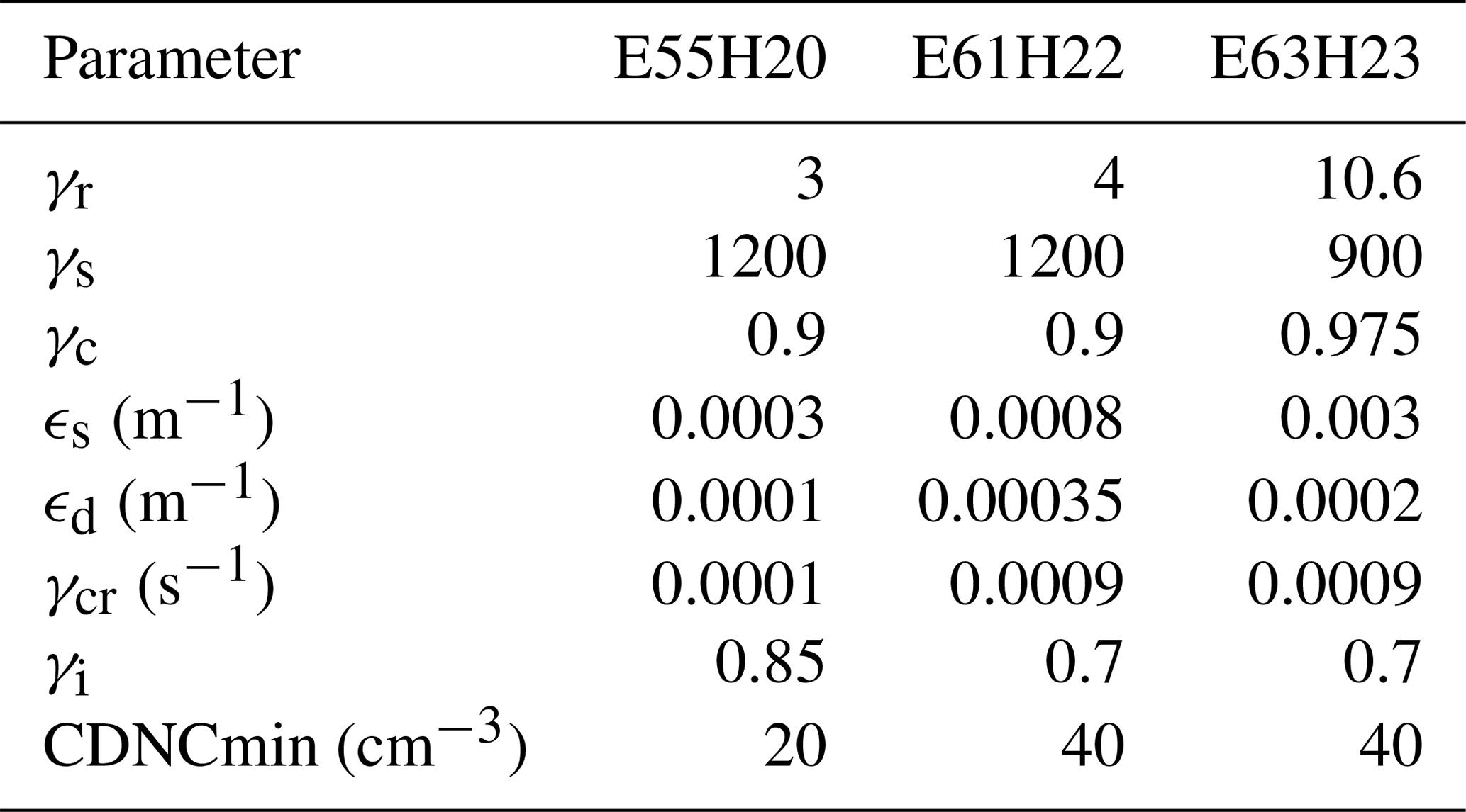
Table 2Parameter settings for E55H20, E61H22 ,and E63H23. The parameters used to tune the ECHAM–HAM versions are a scaling factor for stratiform rain formation rate by autoconversion (γ_r), a scaling factor for stratiform snow formation rate by aggregation (γ_s), critical relative humidity at the surface, which is used in the cloud cover scheme (γ_c), the entrainment rate for shallow convection (ϵ_s), the entrainment rate for deep convection (ϵ_d), the convective conversion rate from cloud water to rain (γ_cr), an inhomogeneity factor for ice clouds (γ_i), and the minimum cloud droplet number concentration (CDNCmin).

Download Print Version | Download XLSX

The primary tuning target for E63H23 is to match the global mean observed shortwave (SW) and longwave (LW) TOA fluxes within the range of uncertainty of the observations along with a TOA net radiative imbalance close to the observed present-day value. The secondary tuning target is that the SW, LW, and TOA net cloud radiative effect (CRE) are within the range of uncertainty of the observations. Cloud cover (CC), liquid water path (LWP), ice water path (IWP), total precipitation (P), and aerosol optical depth (AOD) should also be close to the range of observed values (see Table 3).

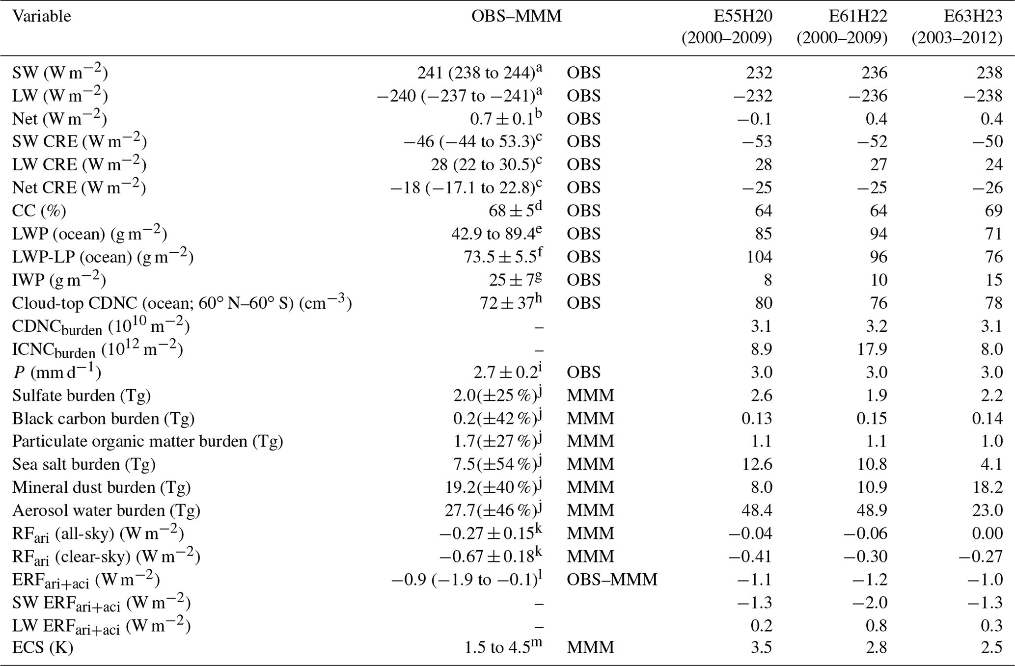
Table 3Global mean values of the PD simulations. Radiative fluxes are at the top of the atmosphere. Values from observations (OBS) and multi-model means (MMMs) for aerosol burdens are shown next to those of the three model versions. ERF_ari+aci and ECS are from the PD_aer ∕ PI_aer and 1xCO₂∕2xCO₂ simulations, respectively.

^a Central values from Loeb et al. (2018), range from Stevens and Schwartz (2012). ^b Loeb et al. (2018) and Johnson et al. (2016). ^c Central values from Loeb et al. (2018); the range takes into account values from Loeb et al. (2009) and Matus and L'Ecuyer (2017). ^d Stubenrauch et al. (2013). ^e Platnick et al. (2015, 2017), ATSR2-AATSR v2.0 (Stengel et al., 2017a; Poulsen et al., 2017), Elsaesser et al. (2017). ^f Elsaesser et al. (2017). ^g Li et al. (2012). ^h Bennartz and Rausch (2017). ⁱ Central value from Adler et al. (2018),
uncertainty from Adler et al. (2012). ^j Taken from Table 10 of Textor et al. (2006). ^k Taken from Table 3 of Myhre et al. (2013). ^l Boucher et al. (2013). ^m Collins et al. (2013),
Knutti et al. (2017).

Download Print Version | Download XLSX

The tuning is done with short 1-year simulations with a climatology for SST and sea ice. When a set of parameters has been found, one or more 10-year simulations are done to minimize the uncertainty in TOA net radiative imbalance. For E61H22 the default parameter values are used (Neubauer et al., 2014). For E55H20 it was necessary to retune the model with the tuning strategy described above, as the tuning in Zhang et al. (2012) was undertaken for nudged simulations, and we performed free simulations to compare the three ECHAM–HAM model versions. The largest differences in tuning between the three model versions are in the tuning parameters for the autoconversion of cloud droplets to rain and entrainment for shallow convection. The latter was adopted from the base model ECHAM6.3 (see Mauritsen et al., 2019, for a discussion of the impact of the change in this tuning parameter on climate sensitivity). In E63H23 stratiform rain formation by autoconversion will be faster than in the other two model versions. This is due to the larger value of the respective tuning parameter leading to reduced LWP, CC, and SW CRE and a more positive TOA net radiative imbalance in E63H23 (Lohmann and Ferrachat, 2010). The larger value of the tuning parameter for entrainment for shallow convection in E61H22 and the even larger value in E63H23 have the opposite effect: increased LWP, CC, and SW CRE and a more negative TOA net radiative imbalance (Mauritsen et al., 2012). For E63H23 there is a compensation by changing both tuning parameters; the most pronounced net effect is a reduced LWP compared to the other two model versions (we hypothesize that LWP is reduced since entrainment for shallow convection mainly affects low, thin clouds, whereas the autoconversion rate affects all liquid clouds; since the reflectivity of clouds depends nonlinearly on their thickness, an increase in thin low clouds can compensate for the SW CRE change with a decrease in thicker clouds but lead to a lower global mean LWP).

2.4 Observational products

We list the products and the respective references for the observational products used in the model evaluation. From Moderate-resolution Imaging Spectroradiometer (MODIS Aqua) collection 6.1 (Platnick et al., 2015, 2017) and from the ESA Cloud Climate Change Initiative (CCI) Advanced Very-High-Resolution Radiometer (AVHRR-PM) v3.0 (prototype; Stengel et al., 2017a, b), histograms of cloud-top pressure vs. cloud optical depth and CC are taken. Histograms of cloud-top pressure vs. cloud optical depth were also taken from the International Satellite Cloud Climatology Project (ISCCP; Rossow and Schiffer, 1999; Pincus et al., 2012; Zhang et al., 2012) D1 data. Cloud–Aerosol Lidar and Infrared Pathfinder Satellite Observations (CALIPSO) data for CC are from the GCM-Oriented CALIPSO Cloud Product (GOCCP) dataset (Chepfer et al., 2010). Cloud radiative effect data are from the Clouds and the Earth's Radiant Energy System (CERES) Energy Balanced and Filled (EBAF) TOA edition 4.0 data product (Loeb et al., 2018). Precipitation data are from the Global Precipitation Climatology Product (GPCP) 2.3 (Adler et al., 2018). Cloud-top CDNCs are from the climatology of Bennartz and Rausch (2017). LWP data are from the Multi-Sensor Advanced Climatology of LWP (MAC-LWP; Elsaesser et al., 2017), which is an updated version of the University of Wisconsin LWP climatology, and from MODIS. IWP is from satellite observations compiled by Li et al. (2012).

3.1 Global mean comparison to observations

Table 3 includes global mean values of radiation, cloud, and aerosol-related variables of the PD simulations of E55H20, E61H22, and E63H23 compared to observations (OBS) or multi-model mean (MMM) values when observations are not available. The global mean values of the radiative fluxes shown in Table 3 are tuning targets (see Sect. 2.6) and therefore cannot be used directly for model evaluation. For E63H23 the SW and LW TOA fluxes, as well as the SW and LW TOA CRE, are within the range of the observations. The net TOA flux of E63H23 is also close to the observations (additional tuning could bring it closer to the observed value but was not attempted given the large uncertainty in, e.g., SW and LW TOA fluxes). The SW, LW, and net TOA fluxes of E61H22 and E55H20 are outside the range of observations. This reflects the change in the tuning targets and strategy in E63H23 and the availability of better observations. The net CRE of E63H23 (and also E55H20 and E61H22) is outside the observed range. It was not possible to find parameter settings that bring the net CRE within the range of observations without bringing one or more of the other radiative fluxes outside the range of observations. This is a first indication of a structural problem in ECHAM–HAM, which could be related to how ice crystals nucleate in (warming) cirrus clouds or an underestimation of (cooling) stratocumulus. This will be further discussed in the evaluation. The CC, P, and cloud-top cloud droplet number concentration (CDNC) of all three model versions agree fairly well with observations (for cloud-top CDNC of the model simulations we selected CDNC over ocean only of the topmost layer of clouds with a cloud-top temperature >273.15 K). For LWP a climatology based on microwave sensors (Elsaesser et al., 2017) provides reliable observations as long as the ratio of LWP to LWP+rainwater path is large (>0.8 is used here), i.e., in regions with relatively low precipitation. The values of LWP only in this low precipitation region (LWP-LP) are also shown in Table 3. Whereas the mean values over the global oceans for LWP and LWP-LP of E61H20 and E55H20 are higher than observed, E63H23 shows values within the observational range (71 and 76 g m⁻², respectively). This is due to the more physically based activation scheme in E63H23 and improvements in ECHAM6.3 like energy conservation in the physics part and improvements in the cloud cover scheme for marine stratocumulus clouds, which allow for an increase in the tuning parameter for autoconversion (see Table 2). Similarly, the global mean value of IWP in E63H23 with 15 g m⁻² is only slightly below the observational range (18–32 g m⁻²), whereas in E61H22 and E55H20 IWP is considerably smaller (10 and 8 g m⁻², respectively). This is because in the accretion of ice crystals by snow, the sticking efficiency follows Seifert and Beheng (2006) in E63H23, whereas in E55H20 and E61H22 it followed Levkov et al. (2012). The Seifert and Beheng (2006) sticking efficiency leads to a less efficient removal of ice crystals by snow. Furthermore, the changed sticking efficiency allows for a reduction of the stratiform snow formation rate by aggregation compared to earlier model versions (see Table 2), which also increases IWP. The aerosol mass burdens of the five prognostic aerosol species in ECHAM–HAM are within the range of AeroCom models (Textor et al., 2006), except for particulate organic matter (POM). This may be related to the simplistic treatment of secondary organic aerosol (SOA) in all three model versions in the experiments for this study. Details on the evaluation of E63H23 with respect to atmospheric aerosol are given in Tegen et al. (2019).

3.2 Zonal mean comparison to observations

Although the global mean values are tuning targets (see Sect. 2.6), biases in net CRE and IWP in the ECHAM–HAM versions, which could not be brought in agreement with observations via tuning, were identified in the previous section. Zonal mean values of observable variables can nevertheless be used for model evaluation because tuning targets the global mean quantities. Figure 1 shows zonal mean distributions of several quantities for the three model versions and observations. The zonal distribution of SW CRE and LWP-LP of E63H23 agrees relatively well with observations, whereas in E61H22 and E55H20 the magnitude of both quantities is overestimated in midlatitudes. The cloud cover distribution of E63H23 also agrees well with observations, whereas E61H22 and E55H20 show an underestimation by up to 10 percentage points in the subtropics. Biases in cloud-top CDNC are more complex, and retrievals of cloud-top CDNC are only possible for specific clouds (e.g., horizontally homogeneous, unobscured, optically thick clouds) and rely on assumptions, such as liquid water content increasing with altitude like in an adiabatically rising cloud parcel (or at least like a constant fraction of this liquid water content), CDNCs being constant throughout the cloud, and further assumptions that together make cloud-top CDNC retrievals uncertain (Grosvenor et al., 2018). We therefore expect larger differences between observations and models for cloud-top CDNC than for other variables. E55H20 agrees well with MODIS observations in the tropics but overestimates cloud-top CDNC in the subtropics on both hemispheres and midlatitudes in the Southern Hemisphere. E61H22 overestimates cloud-top CDNC in the tropics and subtropics but underestimates it at midlatitudes in the Northern Hemisphere. E63H23 also overestimates cloud-top CDNC in the subtropics, but less than E61H22, and also in the tropics. The liquid phase of clouds is therefore better represented in E63H23 than in the previous model versions. IWP is underestimated in all three model versions. E63H23 has the smallest bias, followed by E61H22, and E55H20 shows the largest deviation from observed zonal mean IWP. The underestimation is particularly large in the tropics, which is likely connected to the parameterization of convection in ECHAM (and ECHAM–HAM). ECHAM has a low precipitation bias over land in the tropics (Mauritsen et al., 2012; Stevens et al., 2013). Gasparini et al. (2018) found indications that the level of detrainment from deep convection is too low in altitude in ECHAM–HAM. They lowered the tuning parameter for deep convective entrainment ϵ_d to 0.00006, whereas all three ECHAM–HAM versions used here have to use a larger value for this parameter (Table 2) as they use a cirrus scheme in which cirrus clouds can only nucleate homogeneously, which may lead to an overestimation of ICNC and an underestimation of IWP by tuning of radiative fluxes (see Sect. 3.3). For LW CRE (and precipitation and AOD, not shown) all three model version differences are within the range of different observational products. In the tropics E55H20 has a rather strong LW CRE, whereas E63H23 and E61H22 have a rather weak LW CRE, but all are within the range of observations.

Figure 1Comparison of zonal annual mean values of E55H20, E61H22 and E63H23 to observations, (a) SW CRE, (b) LWP-LP over oceans, (c) LW CRE, (d) IWP, (e) total cloud cover, and (f) cloud-top CDNC of clouds between 268 and 300 K over oceans. Observations of IWP are from Li et al. (2012), LWP-LP over oceans from Elsaesser et al. (2017), cloud-top CDNC over oceans from Bennartz and Rausch (2017). The solid SW and LW CRE lines are from CERES (Loeb et al., 2018), the dashed ones from ERBE (Barkstrom, 1984), and the dotted one for LW CRE is from TOVS satellite data (Susskind et al., 1997). Total cloud cover is from CALIPSO GOCCP (solid line; Chepfer et al., 2010), AVHRR-PM (dashed line; Stengel et al., 2017b), and MODIS collection 6.1 (dotted line; Platnick et al., 2015, 2017).

Download

3.3 Regional comparison to observations

The comparison of CRE of the different model versions with CERES CRE reveals several biases in the representation of clouds. We therefore start by identifying biases in CRE and then use observations for other quantities to identify the causes of the model biases. In Fig. 2 the differences in SW, LW, and net TOA CRE of all model versions to CERES observations are shown. In all three model versions the (negative) SW CRE is too weak in the marine stratocumulus regions west of the continents (the average bias in the wider stratocumulus regions is 1.1, 8.1, and 7.0 W m⁻² in E63H23, E61H22, and E55H20, respectively). In addition, the SW CRE is too weak in some land areas in E63H23 and E61H22, in the Southern Ocean in E63H23, and in the tropical oceans in E55H20 (3.3 W m⁻² average bias over ocean between 15^∘ N and 15^∘ S, excluding wider stratocumulus regions). These biases are compensated for by a stronger SW CRE over large parts of the oceans and middle- and high-latitude land areas in the Northern Hemisphere. The bias in stratocumulus regions is smaller in E63H23 than in the older model versions and so are the compensating negative biases. This is due to improvements in ECHAM6.3 like improvements in the cloud cover scheme for marine stratocumulus clouds. The (positive) LW CRE is too weak in the tropics in E63H23 and E61H22 (−7.7 and −4.8 W m⁻² average bias, respectively, between 20^∘ N and 20^∘ S, excluding wider stratocumulus regions) and too strong in the tropics (in particular over land) in E55H20 (1.2 W m⁻²). Together with the biases in the tropical SW CRE this points to problems with the parameterization of deep convective clouds, detrained condensate, or the representation of anvils from detrained condensate in all three model versions. In all three model versions the LW CRE in midlatitudes is too weak (except over land in the Northern Hemisphere). At high latitudes it is stronger than in the CERES data in all model versions (but the uncertainty of CERES CRE is also larger at high latitudes; Loeb et al., 2018). Only a few of the biases in SW and LW CRE compensate, and therefore the biases in net CRE are as large as or larger than in the SW (LW) CRE. In the net CRE the positive biases in stratocumulus regions and in the Southern Ocean in E63H23 and E61H22, over land in E61H22, and in the tropical oceans in E55H20 are compensated for in the global mean by negative biases in all other regions. The negative biases are caused by adjusting cloud parameters to bring the global mean values in agreement with observations. Therefore, if the biases in stratocumulus regions and the Southern Ocean (and the tropics) could be reduced, the negative biases in SW and net CRE would also be smaller.

Figure 2Comparison of annual mean SW, LW, and net CRE of E55H20, E61H22, and E63H23 to CERES 4.0 (Loeb et al., 2018) observations. CERES data are for 2005–2015, model data are from the PD simulations. In the top left panel the regions used for cloud-top pressure vs. cloud optical depth histograms are shown by green lines.

In Fig. 3 the cloud cover of the CALIPSO GOCCP product and all three model versions is shown. The hatched areas in Fig. 3 are the regions where the cloud cover of CALIPSO GOCCP, MODIS collection 6.1, and ESA Cloud CCI (AVHRR-PM) differs by more than five percentage points. We therefore use only the areas not marked by hatching in Fig. 3 for the model evaluation. Since the COSP CALIPSO simulator is not implemented in E55H20, the direct model output is shown for all model versions (see Fig. S8 for COSP CALIPSO simulator output of cloud cover for E61H22 and E63H23). The cloud cover of all three model versions agrees fairly well with the observations. The largest biases are in stratocumulus regions west of the continents (−10, −18, and −22 percentage points in E63H23, E61H22, and E55H20, respectively, in the wider stratocumulus regions), where the models underestimate the cloud cover. Over land in the Northern Hemisphere poleward of about 45^∘ N the models overestimate cloud cover, and in the Indonesian warm pool region the cloud cover is biased high in the three model versions. The underestimation of cloud cover in stratocumulus regions is less severe in E63H23 than in the other two model versions (the cloud cover scheme in ECHAM6.3 was improved to better represent cloud cover in these regions).

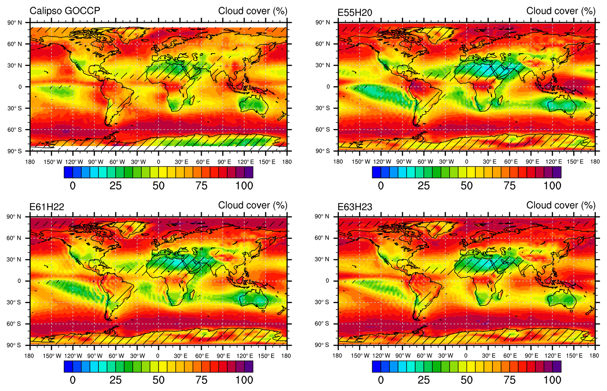
Figure 3Comparison of annual mean cloud cover of E55H20, E61H22, and E63H23 to CALIPSO GOCCP observations. Areas where the cloud cover of CALIPSO GOCCP, MODIS collection 6.1, and AVHRR-PM differ by more than five percentage points are hatched. CALIPSO GOCCP data are for 2006–2010, model data are from the PD simulations (direct model output is used without a simulator).

Figure 4 shows LWP from the MAC-LWP climatology (Elsaesser et al., 2017) and the three model versions. The retrieval of LWP has biases from both visible and near-infrared sensors as well as microwave sensors (Seethala and Horváth, 2010; Lebsock and Su, 2014). Visible and near-infrared sensors such as MODIS have problems when the solar zenith angle is large and detecting pixels of clouds at low altitudes (Lebsock and Su, 2014). Microwave sensors such as AMSR-E may retrieve LWP in cloud-free scenes, and the split between LWP and rainwater path is difficult (Lebsock and Su, 2014). Elsaesser et al. (2017) corrected the retrieval bias of LWP of microwave-sensor-based products in cloud-free scenes. And they recommend using regions with low precipitation (LWP∕(LWP+rainwater path) >0.8) for model evaluation. The regions where precipitation could influence the LWP retrieval are therefore hatched in Fig. 4. This leaves the stratocumulus regions west of the continents and the storm tracks over ocean in the Northern and Southern Hemisphere as the most reliable areas for the evaluation of LWP. All three model regions show a fairly good agreement of LWP in the stratocumulus regions except west of South America and southwest Africa, where all model versions tend to underestimate LWP. In the storm tracks over ocean in the Northern and Southern Hemisphere, on the other hand, E61H22 and even more E55H20 overestimate LWP. E63H23 instead shows a rather good agreement of LWP in the storm tracks compared to observations. This is likely the result of different model tuning in E63H23 (see Sect. 2.3), which was possible due to a more realistic geographic pattern of cloud cover and SW CRE in E63H23.

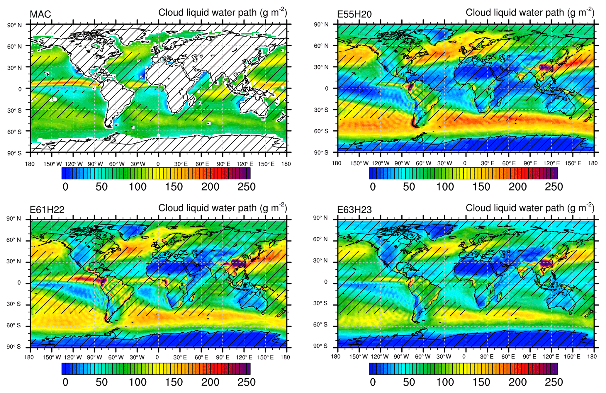
Figure 4Comparison of annual mean LWP of E55H20, E61H22, and E63H23 to MAC-LWP observations. Areas where precipitation could influence the LWP retrieval (LWP∕(LWP+rainwater path) ≤0.8) are hatched. MAC data are for 2003–2012, model data are from the PD simulations.

To further characterize the simulation of liquid clouds in the ECHAM–HAM model versions we also compare cloud-top CDNC of warm (cloud top warmer than 0 ^∘C) liquid clouds to the cloud-top CDNC from Bennartz and Rausch (2017), which is based on MODIS Aqua data (Fig. 5). The hatched area marks regions where the relative uncertainty in the observations is larger than 75 %. The general geographical distribution and magnitude of cloud-top CDNC of all model versions agree with the observations, although there are certain areas where model biases are apparent. E61H22 has lower cloud-top CDNCs in midlatitude ocean regions than E63H23; in E55H20 they are higher than in the other two model versions. In E55H20 the higher cloud-top CDNCs can be explained by reduced entrainment of deep convection (see Table 2) compared to the other model versions, which leads to higher relative humidity in the upper tropical troposphere that subsequently leads to increased aerosol nucleation, more Aitken mode particles, and increased CCN concentrations. E63H23 uses the Abdul-Razzak and Ghan (2000) activation scheme and the Long et al. (2011) sea salt emission parameterization (temperature dependent; Sofiev et al., 2011), which lead to higher cloud-top CDNCs than in E61H22 (which uses the Lin and Leaitch, 1997, activation scheme and the Guelle et al., 2001, sea salt emission parameterization) despite the lower LWP in E63H23. Furthermore, in subtropical regions where the cloud cover and LWP are low (see Figs. 3 and 4), cloud-top CDNCs are higher in all three model versions than in the observations. In these regions, shallow trade-wind cumulus clouds occur frequently (Medeiros and Stevens, 2011), and in all model versions shallow convection is triggered frequently (see Fig. S2). The weighted average of stratiform CDNC and detrained CDNC (see Sect. 2.1.3) may overestimate the CDNC of shallow cumulus clouds. The use of a two-moment cloud microphysics scheme for convective clouds (e.g., Lohmann, 2008) so that CDNC in convective clouds can be reduced by collision–coalescence, or a different way to account for detrained CDNC, could help to alleviate this model bias. All three model versions also underestimate cloud-top CDNC at high latitudes. As retrievals from visible and near-infrared sensors often have biases at large zenith angles (see above) this may be a problem with the observations.

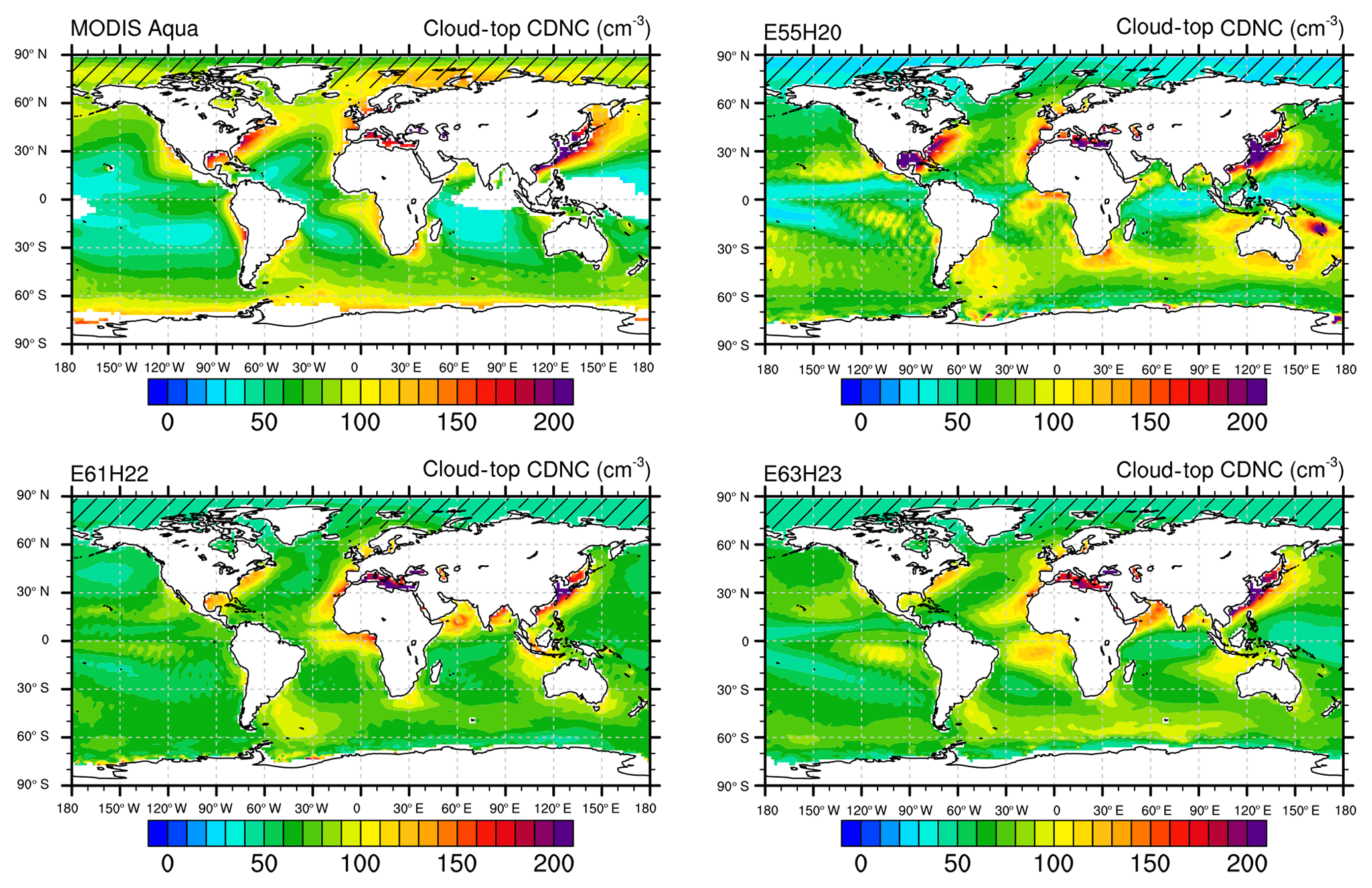
Figure 5Comparison of annual mean cloud-top CDNC of E55H20, E61H22, and E63H23 to MODIS observations from Bennartz and Rausch (2017). Areas where the relative uncertainty in the observations is larger than 75 % are hatched. The MODIS data are for 2003–2015, model data are from the PD simulations.

In Fig. 6 the IWP of all three model versions and IWP satellite observations compiled by Li et al. (2012) are shown. Li et al. (2012) used three different CALIPSO plus CloudSat ice water products and two different methods to remove the contribution of convective clouds and precipitation from the products. Figure 6 displays the compiled mean IWP of the datasets of Li et al. (2012), and areas where the relative standard deviation of the different datasets is larger than 75 % are hatched. The regional distribution of the occurrence of IWP of all three model versions agrees in general quite well with the observations, although it is biased low in all ECHAM–HAM model versions. This could already be seen in the respective global mean and zonal mean values (see Sect. 3.1 and 3.2). Similar to what was found in the analysis of zonal mean IWP the underestimation is largest in the tropics (see Sect.  3.2).

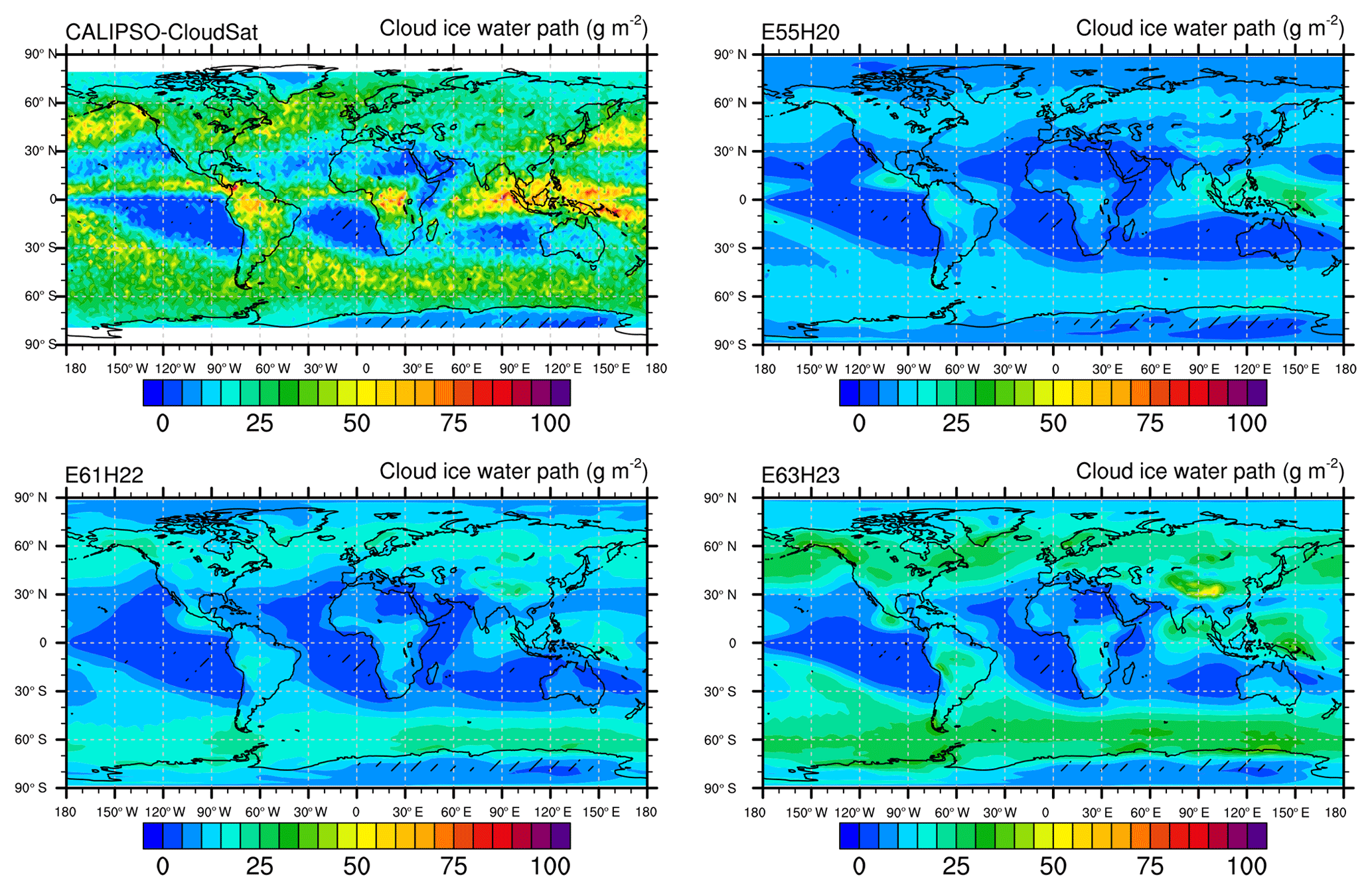
Figure 6Comparison of annual mean IWP of E55H20, E61H22, and E63H23 to CALIPSO–CloudSat observations from Li et al. (2012). Areas where the relative standard deviation of the different datasets compiled in Li et al. (2012) is larger than 75 % are hatched. The CALIPSO–CloudSat data cover the years 2006–2010, model data are from the PD simulations.

Cloud ice mass vertical profiles can be obtained from CALIPSO plus CloudSat observations. The global mean vertical profile of ice water content (IWC) is shown in Fig. 7 for all three model versions and the compiled mean IWC from Li et al. (2012). IWC is underestimated above 700 hPa in all model versions. In E63H23 the maximum of IWC is at the same pressure level as in the observations, at about 350 hPa, whereas in E61H22 and E55H20 the maximum of IWC is at higher altitudes at about 300 to 250 hPa. This can be explained by changes in ICNC and subsequent changes in precipitation formation and ice crystal sedimentation. ICNC changed between the model versions because the way detrained ice crystals are added to existing stratiform clouds has changed since E61H22. The shape of the ice crystals has been made consistent in all modules since E61H22, and a bug in E61H22 was removed in E63H23, which led to homogeneous freezing of dry aerosol particles independent of the availability of water vapor below −35 ^∘C (the latter improvement was most important as it doubled the ICNC burden in E61H22 compared to the other two model versions; see Table 3). Below 700 hPa the three model versions are close to the observed IWC, with E63H23 showing an overestimation of IWC and E55H20 an underestimation.

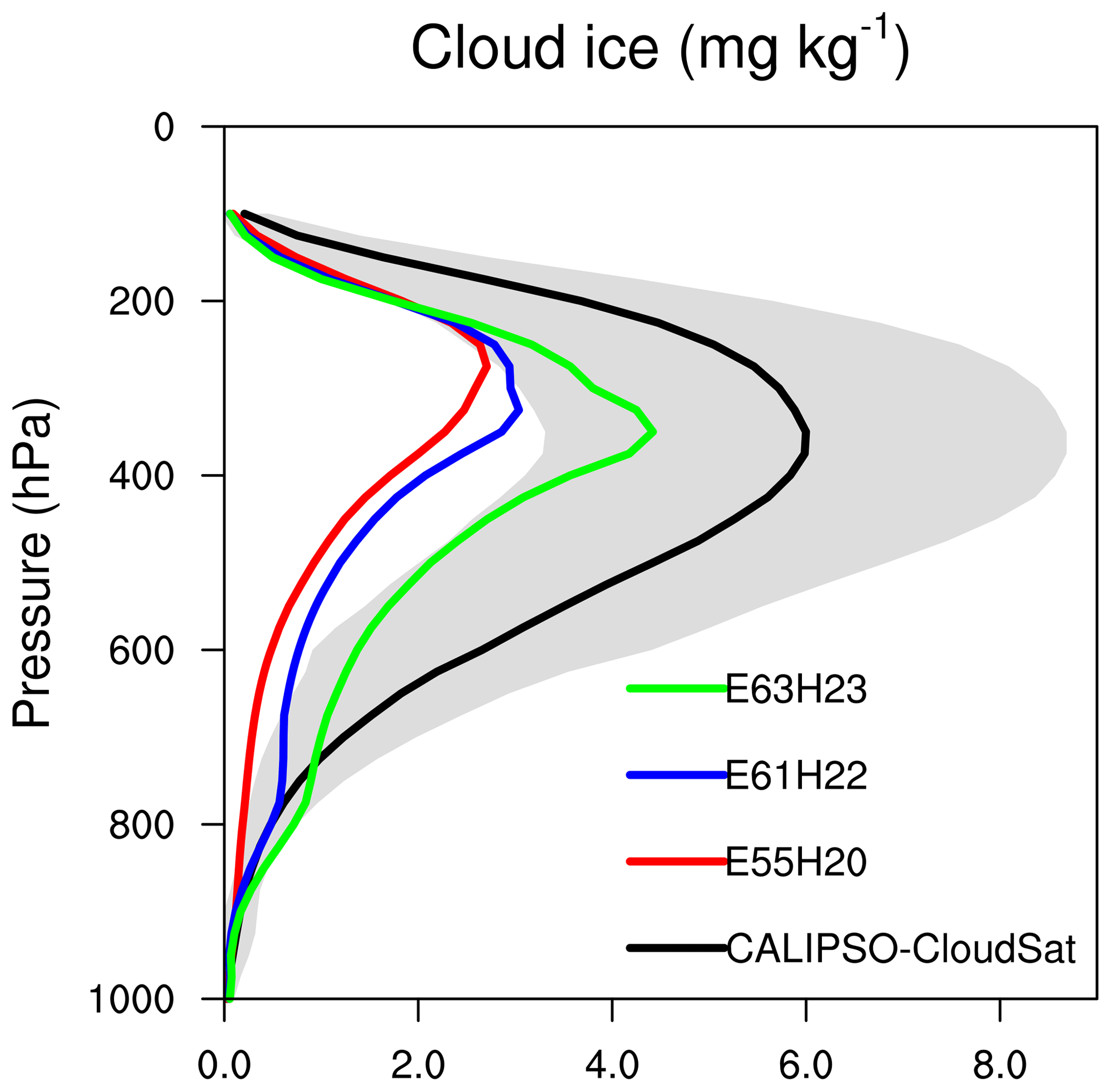
Figure 7Comparison of global annual mean IWC as a function of pressure of E55H20, E61H22, and E63H23 to CALIPSO–CloudSat observations from Li et al. (2012). Gray shading indicates the uncertainty in the CALIPSO–CloudSat observations. The CALIPSO–CloudSat data cover the years 2006–2010, model data are from the PD simulations.

Download

The regions where IWP is underestimated in the three model versions correspond to the regions where the three model versions underestimated LW CRE in Fig. 2 (in particular in the tropics). There are also regions where LW CRE is overestimated (see Fig. 2) in the three model versions, although IWP is underestimated (see Fig. 6). This is an indication that ICNC is too large in the three model versions (the vertical profile of IWC agrees fairly well with observations, although the IWC magnitude is underestimated in all three model versions). As IWP is larger in E63H23 than in E61H22 and E55H20 but the overestimation in LW CRE is smaller in E63H23 than in E61H22 and E55H20, this is an indication that ICNC and the size of the ice crystals are closer to reality in E63H23 than in E61H22 and E55H20. The overestimation of LW CRE in E61H22 around 60^∘ N and 60^∘ S can be explained by the high ICNC in E61H22 (see Table 3) caused by the ICNC bug mentioned above.

Next to E61H22 there is also a bias of net CRE south of 60^∘ S in E63H23 (see Fig. 2). This is not due to ICNC that is too high, as LW CRE of E63H23 agrees well with CERES observations in this region. In E63H23 there is an underestimation of SW CRE south of 60^∘ S. Cloud cover and IWP of E63H23 agree well with observations in this region. LWP is slightly underestimated, but cloud-top CDNC is strongly underestimated. Either there is a problem with the satellite retrievals at these high southern latitudes or E63H23 is missing liquid clouds in this region. In E61H22 and E55H20 this possible bias south of 60^∘ S is hidden by the overestimation in LWP, which leads to a stronger SW CRE.

In Fig. 8 the total precipitation of all model versions and GPCP2.3 (Adler et al., 2018) is shown. Areas where the relative uncertainty of the GPCP2.3 data is larger than 75 % are hatched. Despite the biases in the representation of clouds in the three model versions identified above, the geographical distribution and magnitude of the annual mean precipitation of all model versions agree well with the observations. Only in the intertropical convergence zone (ITCZ) and South Pacific convergence zone (SPCZ) do the areas and magnitude of precipitation differ from the observations, corresponding to differences in cloud cover and IWP (Figs. 3 and 6, respectively). Cloud cover, IWP, and precipitation are low in the central Pacific and central Atlantic ITCZ but relatively large in the ITCZ west of Central America, east of South America, over the Philippines, and west of Southeast Asia. In the SPCZ cloud cover, IWP, and precipitation are relatively large compared to the respective observations. ECHAM underestimates tropical precipitation over land and overestimates tropical precipitation over ocean (Mauritsen et al., 2012; Stevens et al., 2013). This bias can also be seen in Fig. 8 for all ECHAM–HAM versions. Since ECHAM and ECHAM–HAM use the same parameterizations for convective clouds, this bias is very likely inherited from the base model ECHAM.

Figure 8Comparison of annual mean precipitation (stratiform + convective) of E55H20, E61H22, and E63H23 to GPCP2.3 observations. Areas where the relative uncertainty of the GPCP2.3 data is larger than 75 % are hatched. The GPCP2.3 data are for 1979–2017, model data are from the PD simulations.

In Fig. 9 histograms of cloud-top pressure vs. cloud optical depth of ECHAM–HAM are compared to ISCCP, AVHRR-PM, and MODIS observations. The COSP simulator (Bodas-Salcedo et al., 2011) was not implemented in E55H20 so we only compare E61H22 and E63H23 to the observations. We applied the COSP–ISCCP simulator for E61H22 and E63H23 for comparison to ISCCP and AVHRR-PM. The COSP–MODIS simulator is only implemented in E63H23 so we compare only E63H23 to MODIS. The histograms were produced for four regions (shown in Fig. 2): wider stratocumulus regions, midlatitudes, tropics, and 60^∘ N to 60^∘ S. The five marine stratocumulus regions are west of North and South America, west of northern and southern Africa, and west of Australia. The marine stratocumulus regions are extended to the west to approximately cover the regions where the three model versions underestimate SW CRE (see Fig. 2). The midlatitude regions are 60 to 20^∘ N and 20 to 60^∘ S, excluding the areas covered by the wider stratocumulus regions. The tropics are between 20^∘ N and 20^∘ S, excluding the areas covered by the wider stratocumulus regions. The region 60^∘ N to 60^∘ S is the sum of the wider stratocumulus, midlatitudes, and tropics; 60^∘ N to 60^∘ S was chosen because retrievals from visible and near-infrared sensors often have biases at large zenith angles (see above). Several of the biases described above are also seen in the histograms in Fig. 9. In the region 60^∘ N to 60^∘ S E63H23 and E61H22 simulate too many optically thick clouds and too few optically thin clouds at low and mid-levels compared to the three satellite datasets. Nam et al. (2012) found a similar bias in several fifth-phase Coupled Model Intercomparison Project (CMIP5) models, as did Stevens et al. (2013) in ECHAM6.1 (“too few, too bright”). This bias can also be seen in the midlatitudes and in the tropics. In the wider stratocumulus region, on the other hand, the occurrence of low-level optically thick clouds of E61H22 and E63H23 agrees rather well with those of the three observational datasets. In the wider stratocumulus regions the optically thin low-level (and mid-level) clouds are missing. This agrees with the analysis of SW CRE in that the underestimation in the stratocumulus regions is compensated for by a stronger SW CRE (clouds being optically thicker) in other regions (by model tuning). Therefore, if the bias in stratocumulus regions could be reduced, the biases in SW CRE and cloud optical depth in other regions could also be reduced. In the midlatitudes the optical depth of low-, mid-, and high-level clouds is larger in E61H22 than in E63H23, ISCCP, and AVHRR-PM. This is related to the stronger compensation by tuning for the lack of clouds in stratocumulus regions (the removal of LWP by autoconversion is slower in E61H22 than in E63H23; see Table 2) and to the ICNC bug in E61H22 mentioned above. In the midlatitudes and the tropics there is also a lack of high-level clouds with optical depth between 1.3 and 23 in E63H23 and E61H22. This lack of cirrus clouds corresponds to the underestimation of IWP and LW CRE. Gasparini et al. (2018) evaluated cirrus clouds in a version of E61H22, which included a cirrus cloud scheme that accounts for a competition in cirrus cloud formation by homogeneous nucleation of solution droplets, heterogeneous freezing of ice-nucleating particles, and water vapor deposition on preexisting ice crystals (Kuebbeler et al., 2014). With this cirrus scheme E61H22 could be tuned such that the global mean IWP agrees with the observations compiled by Li et al. (2012). Similarly, Lohmann and Neubauer (2018) made an experiment in which cirrus clouds could only form by heterogeneous freezing of ice-nucleating particles in E63H23. In their experiment this caused the global mean IWP to agree with the observations compiled by Li et al. (2012). These studies and our analysis indicate that the IWP bias in the three model versions occurs because cirrus clouds can only nucleate homogeneously, and therefore ICNC in cirrus clouds and hence their optical properties are misrepresented.

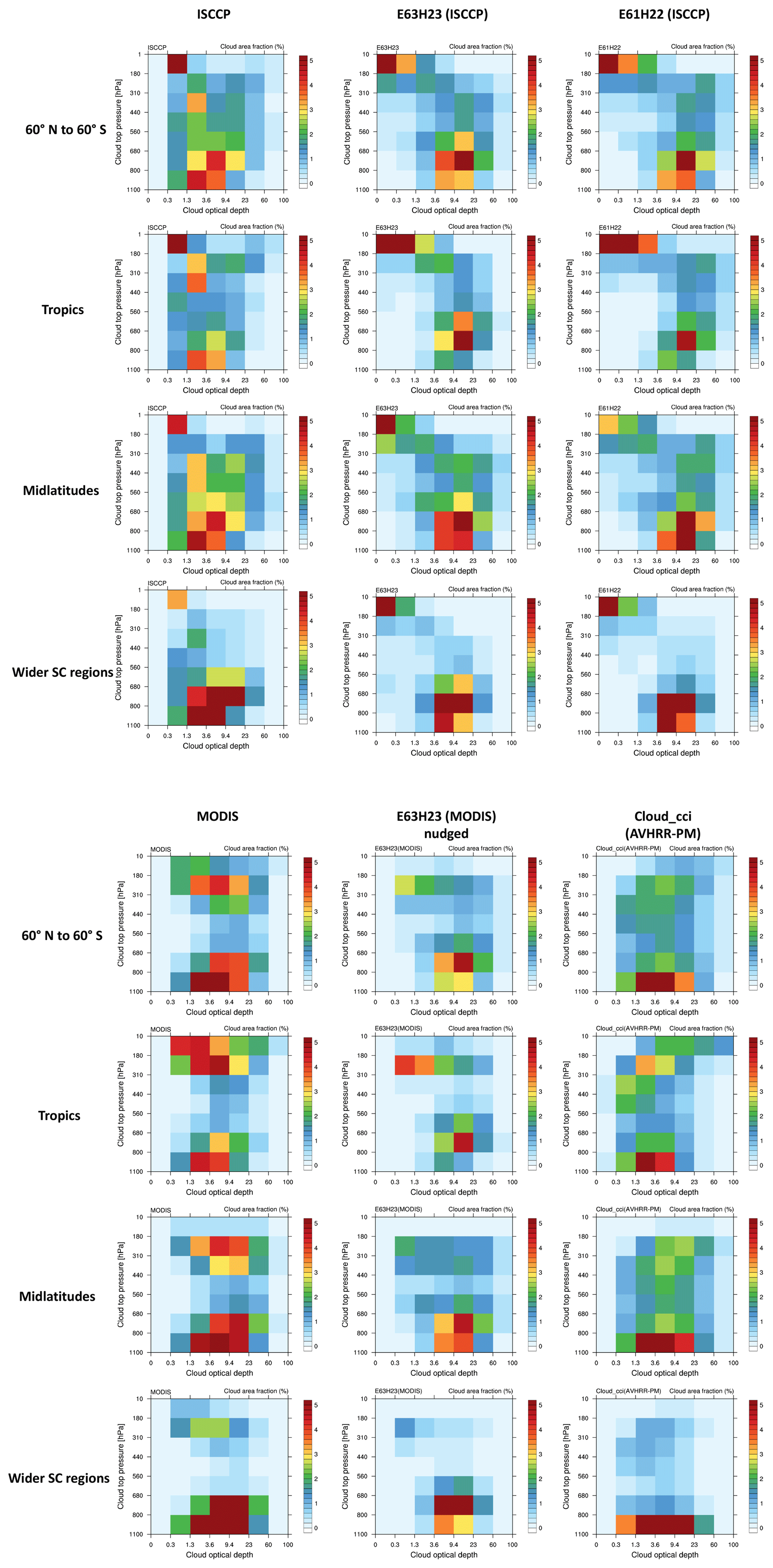
Figure 9Histograms of cloud-top pressure vs. cloud optical depth of E61H22 and E63H23 compared to ISCCP, MODIS, and AVHRR-PM observations for different regions. The definition of the four regions shown is described in the text and the regions are shown in Fig. 2. The ISCCP data are for 2000–2008, MODIS data are for 2003–2012, AVHRR-PM data are for 2003–2012, and the model data are from the PD simulations.

Download

3.4 Summary of model evaluation

Figure 10 shows a Taylor diagram (Taylor, 2001) comparing SW and LW CRE, cloud cover, LWP-LP, cloud-top CDNC, IWP, and precipitation of the three model versions to the respective observations. The standardized deviations of LWP-LP had to be scaled by a factor of 1∕4 so they could fit on the scale. For all variables the root mean square error (RMSE) (solid circles in the diagram in Fig. 10) is smaller than or equal to the RMSE in E63H23 compared to E61H22 and E55H20 (note the scaling for LWP-LP). The changes in the geographical pattern between the three model versions are rather small. E63H23 has somewhat higher correlations except for LW CRE, IWP, and precipitation, for which E55H20 has higher correlations than E63H23 and E61H22. E55H20 has higher correlations of LW CRE, IWP, and precipitation because the ratio of the peaks in these variables in the tropics compared to midlatitudes is better represented in E55H20 (see Fig. 1). Overall, E63H23 is an improvement over earlier model versions.

Figure 10Taylor diagram for comparison of SW and LW CRE, cloud cover, LWP-LP, cloud-top CDNC, IWP, and precipitation of E55H20, E61H22, and E63H23 to observations as REF. The standardized deviations of LWP-LP are scaled by a factor of 1∕4 to fit on the diagram. Only areas that are not hatched in Figs. 3–6 were used to create the Taylor diagram. Observations are the same as in Figs. 2–6 and 8. The correlation coefficient is shown as an angle and quantifies the similarity in pattern between modeled and observed annual mean fields. The standard deviation of the modeled fields (normalized by the standard deviation of the observed fields) is shown as the radial distance from the origin. The RMSE is shown as solid black circles and is the distance from the point marked by REF (the closer a model is to REF, the better its skill in reproducing the observations). For E63H23 and the observations for precipitation and LWP-LP, an average over the time period 2003 to 2012 was used. The following time periods were used: for cloud-top CDNC the time period 2003 to 2015, for IWP the time periods in Li et al. (2012), for SW CRE and LW CRE the time period July 2005 to June 2015, for cloud cover the time period June 2006 to December 2010, and for E55H20 and E63H23 the time period 2000 to 2009. Tests with E63H23 showed a negligible impact of the different time periods for the data in the Taylor diagram.

Download

Several biases in the representation of clouds in the three ECHAM–HAM model versions could be identified. The common problem of GCMs in their representation of convective and boundary layer clouds is also present in the three ECHAM–HAM model versions. Stratocumulus clouds are underestimated in all three model versions. Shallow convective clouds are underestimated in E61H22 and E55H20. In E63H23 the cloud cover and LWP in regions where shallow convective clouds are common agree well with observations, but the cloud-top CDNCs are overestimated, leading to an overestimation of SW CRE in these regions. Deep convective clouds over the Atlantic and Pacific oceans form too close to the continents (see Figs. 3, 6 and 8) in E63H23 and ECHAM (Stevens et al., 2013). For the tropical Atlantic this is a common bias in GCMs with coarse horizontal resolution (Siongco et al., 2014). Siongco et al. (2017) discuss different ways this bias in the tropical Atlantic precipitation could be reduced in ECHAM6. IWP is underestimated in all three model versions, in particular in the tropics, whereas LW CRE and the vertical profile of cloud ice agree rather well with observations. This indicates that ICNC may be overestimated in all three model versions (since LW CRE depends on the cloud temperature (∼ cloud altitude) and cloud optical depth: ∝ ICNC, IWP). As E63H23 has the smallest bias in IWP, the bias in ICNC should also be smaller than in the previous versions of ECHAM–HAM. Previous studies (Gasparini et al., 2018; Lohmann and Neubauer, 2018) showed that this overestimation of ICNC is (at least partly) due to missing processes in the formation of cirrus clouds (heterogeneous freezing of ice-nucleating particles and/or water vapor deposition on preexisting ice crystals). These studies also showed that including these processes can reduce the underestimation of IWP in ECHAM–HAM. South of 60^∘ S LWP and cloud-top CDNC of E63H23 could be underestimated, although there could also be problems with the satellite retrievals at these high latitudes. In the previous model versions this possible bias was hidden by the overestimation of LWP.

3.5 Simulation of ERF_ari+aci, RF_ari, and ECS

In Fig. 11 global maps of SW and LW ERF_ari+aci for E63H23, E61H22, and E55H20 are shown. An important difference exists in the setup of E55H20 and the two other model versions. E55H20 uses AeroCom I aerosol emission data and the years 1750 and 2000 for preindustrial and present-day aerosol emissions. E63H23 and E61H22, on the other hand, use AeroCom II aerosol emissions and the years 1850 and 2008 for preindustrial and present-day aerosol emissions. The stronger SW ERF_ari+aci in the east of North America and Europe and the weaker SW ERF_ari+aci in South and East Asia in E55H20 compared to the two other model versions are therefore predominantly the result of the different representative emission years and inventories (see Supplement Fig. S3). We keep these emission years as they were used as the default in previous studies (e.g., Zhang et al., 2012; Neubauer et al., 2014).

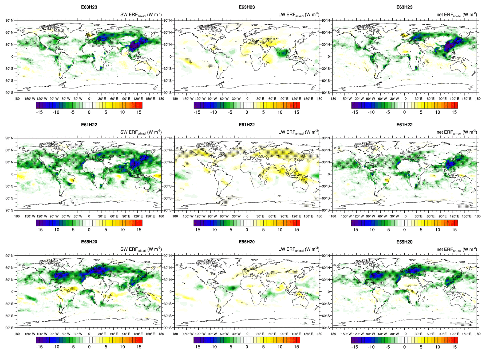
Figure 11Global maps of SW, LW, and net ERF_ari+aci of E55H20, E61H22, and E63H23 from 20-year free simulations with present-day minus preindustrial aerosol emissions (PD_aer − PI_aer). Hatching indicates statistically significant differences at the 95 % significance level. The false discovery rate is controlled following Wilks (2016).

The treatment of surface albedo over land, ocean, and sea ice has changed substantially from ECHAM5 to ECHAM6 (see Stevens et al., 2013), which has an impact on SW ERF_ari+aci (Stier et al., 2013). Because of the differences in the setup and surface albedo treatment of E55H20 we focus the comparison of ERF_ari+aci on differences between E61H22 and E63H23. ERF_ari+aci is stronger over land and weaker over oceans in E63H23 compared to E61H22 (Fig. S4). In the global mean 50 % (−0.5 W m⁻²) of ERF_ari+aci originates over land in E63H23 and 50 % (−0.5 W m⁻²) over ocean. This is in contrast to E61H22, wherein 27 % (−0.3 W m⁻²) of ERF_ari+aci originates over land and 73 % (−0.9 W m⁻²) over ocean. E63H23 uses the Köhler-theory-based Abdul-Razzak and Ghan (2000) activation scheme, while E61H22 applies the empirical Lin and Leaitch (1997) activation scheme, which depends only on the number of aerosol particles and updraft velocities. A sensitivity simulation with the Lin and Leaitch (1997) activation scheme applied in E63H23 shows an ERF_ari+aci of 0.4 W m⁻² over land, explaining about half of the difference in ERF_ari+aci over land between E61H22 and E63H23. The increase in ERF_ari+aci in E63H23 over land may also be related to the higher rate of autoconversion in E63H23 (Table 2). While Lohmann and Ferrachat (2010) found no strong dependence of ERF_ari+aci (or a small decrease) on the autoconversion tuning parameters in the global mean, the ratio of autoconversion to the total rain formation rate has a strong regional dependence (see, e.g., Sant et al., 2015), which could lead to regional differences in ERF_ari+aci.

It is interesting to note that although biases in the simulation of clouds in stratocumulus regions are reduced in E63H23, there seems to be no increase in ERF_ari+aci in these regions compared to E61H22. Over the remote oceans, the largest differences in ERF_ari+aci between E63H23 and E61H22 occur between 15 and 45^∘ N, where E61H22 simulates a strong ERF_ari+aci in trade-wind cumulus clouds (Zhang et al., 2016). ERF_ari+aci in these shallow convective clouds regions is weaker in E63H23, although more clouds are simulated in E63H23 in these regions. LWP and cloud cover in E63H23 are closer to observations in these regions (Figs. 3 and 4), and cloud-top CDNCs are rather too high in E63H23 (Fig. 5). A smaller LWP could lead to a weaker ERF_ari+aci (Lohmann and Ferrachat, 2010). To better understand the differences over oceans between E63H23 and E61H22, we also compare E63H23 with a simulation with E63H23 wherein CDNCmin was lowered from 40 to 10 cm⁻³ (E63H23-10CC) as this simulation has a higher LWP (due to retuning with a smaller γ_r=2.8; not shown). Although the smaller CDNCmin of 10 cm⁻³ leads to a stronger ERF_ari+aci everywhere (Hoose et al., 2009; −1.7 W m⁻² in the global mean; Table S1), this simulation still provides useful information. In the Northern Hemisphere Pacific there is an increase in ERF_ari+aci in E63H23-10CC compared to E63H23 (Fig. S5). This may be due to the larger LWP or the change in CDNCmin itself. In the Northern Hemisphere Atlantic, however, ERF_ari+aci does not increase. The weaker ERF_ari+aci in the Northern Hemisphere Pacific in E63H23 could therefore be due to the smaller LWP in this simulation, while the smaller ERF_ari+aci in the Northern Hemisphere Atlantic is due to a different reason. The sensitivity simulation with the Lin and Leaitch (1997) activation scheme applied in E63H23 shows a negative ERF_ari+aci between 15 and 45^∘ N in the Atlantic (Fig. S5). Therefore, the stronger ERF_ari+aci in E61H22 over oceans can be partly explained by the different activation scheme. Another reason for the stronger ERF_ari+aci in E61H22 over oceans between 15 and 45^∘ N is that different sea salt parameterizations are used in E61H22 and E63H23. Tegen et al. (2019) show that the Long et al. (2011) sea salt parameterization (temperature dependent; Sofiev et al., 2011) used in E63H23 leads to higher aerosol number concentrations over ocean compared to the Guelle et al. (2001) sea salt parameterization used in E61H22, improving the agreement with measured sea salt surface concentrations and particle size distributions at different marine sites (see also the comparison of sea salt parameterizations in Zieger et al., 2017). The higher natural background aerosol concentrations due to the higher sea salt aerosol number concentrations in E63H23 also explain why ERF_ari+aci is less negative in E63H23 between 15 and 45^∘ N over oceans than in E61H22 (Fig. S5). From sensitivity simulations with the Lin and Leaitch (1997) activation scheme or the Guelle et al. (2001) sea salt parameterization applied in E63H23 (Table S1) we conclude that the largest part of the change in SW ERF_ari+aci is actually from changes in the base model ECHAM6.3.

Most of the differences between the model versions discussed above are differences in SW ERF_ari+aci. There is one important difference in LW ERF_ari+aci between the model versions. LW ERF_ari+aci is more than twice as large in E61H22 as in E55H20 and E63H23 (Table 3). The stronger LW ERF_ari+aci in E61H22 occurs in Northern Hemisphere midlatitudes and in the tropics (Fig. 12). In Northern Hemisphere midlatitudes LW CRE is also larger in E61H22 due to the ICNC bug (see Fig. 2; ICNC itself is also higher in E61H22; see Table 3). The strong LW ERF_ari+aci in E61H22 is therefore likely an artifact that was removed in the latest model version.

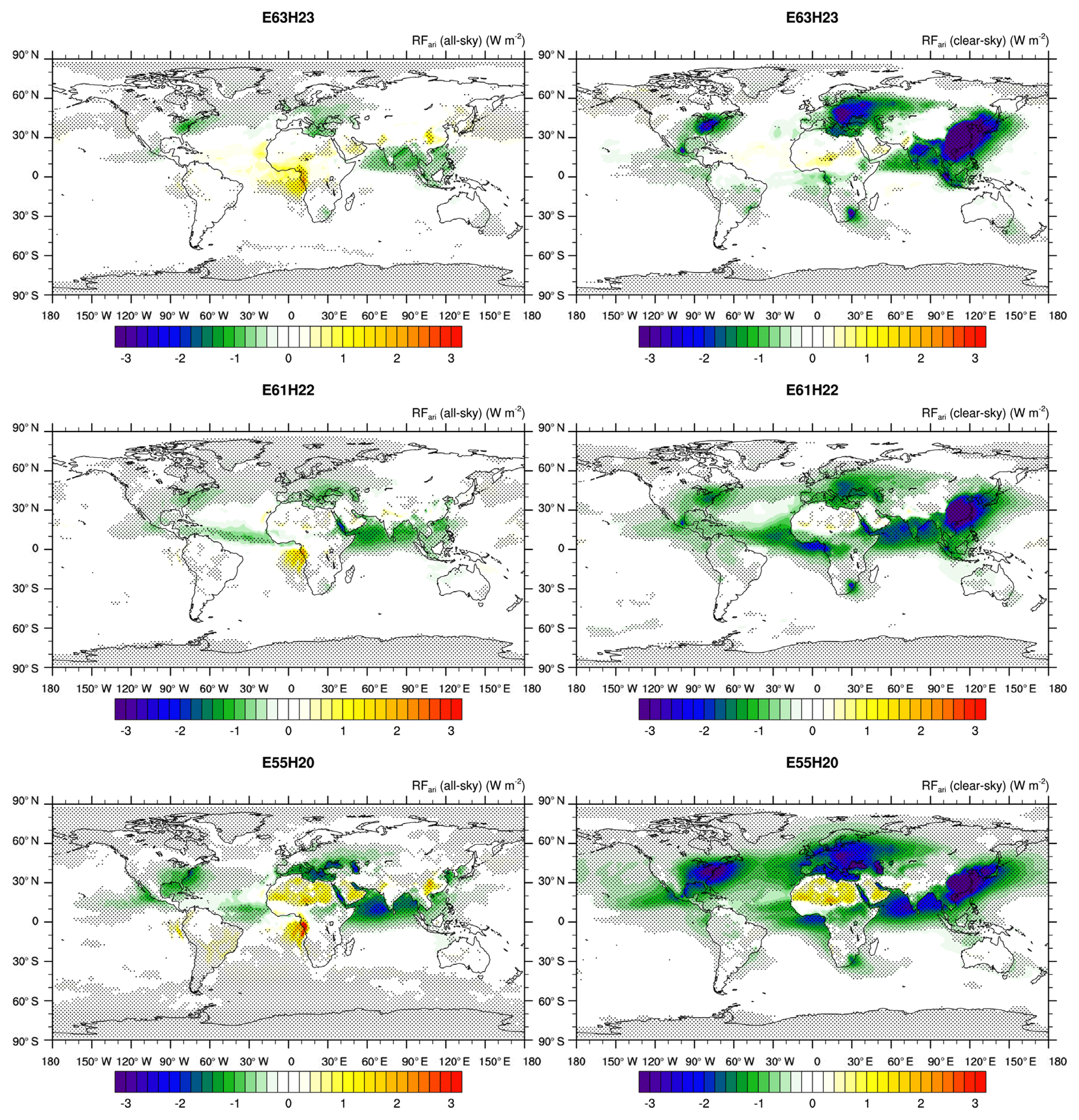
Figure 12 Global maps of all-sky and clear-sky net RF_ari of E55H20, E61H22, and E63H23 from 20-year free simulations with present-day minus preindustrial aerosol emissions (PD_aer − PI_aer). Hatching indicates statistically significant differences at the 99 % significance level. The false discovery rate is controlled following Wilks (2016).

Tegen et al. (2019) found an improved aerosol representation in biomass burning regions when GFAS biomass burning emissions, multiplied by a scaling factor of 3.4 as recommended by Kaiser et al. (2012), replace the default ACCMIP biomass burning emissions. Therefore, we performed an E63H23 simulation with GFAS biomass burning emissions multiplied by 3.4 (E63H23-GFAS34). E63H23-GFAS34 has a weaker ERF_ari+aci (−0.9 W m⁻²) than E63H23 (−1.0 W m⁻²) because the preindustrial aerosol burden is higher in E63H23-GFAS34, and ERF_ari+aci is sensitive to preindustrial aerosol concentrations (Carslaw et al., 2013). Also, the present-day aerosol burdens in E63H23-GFAS34 agree better with the mean aerosol burden of the AeroCom models (Textor et al., 2006) than in E63H23 (see Tables 3 and S1).

We would like to point out that our simulations include interactions between sulfate and mineral dust. On the one hand, (anthropogenic and natural) gaseous sulfate may coat mineral dust particles; this leads to a transfer of dust from insoluble modes to soluble modes in the models, which increases the wet deposition of dust (and leads to decreased present-day mineral dust burdens; see Table S2). On the other hand, mineral dust particles provide surfaces onto which (anthropogenic and natural) gaseous sulfate may condensate, leading to a dampening of the nucleation of new particles. Similar interactions between sulfate and mineral dust have been found by Fan et al. (2004) (using the Geophysical Fluid Dynamics Laboratory (GFDL) global chemical transport model; Mahlman and Moxim, 1978), Bauer and Koch (2005), and Bauer et al. (2007) (using the Goddard Institute for Space Studies (GISS) climate model, modelE; Schmidt et al., 2006; Hansen et al., 2005). The forcing from these interactions between sulfate and mineral dust is included in our estimates for ERF_ari+aci and RF_ari (these interactions will make ERF_ari+aci and RF_ari less negative, but they are difficult to quantify).

RF_ari is shown in Fig. 12 for all-sky and clear-sky conditions for E63H23, E61H22, and E55H20 (since RF_ari is computed by double calls to the radiation scheme, many values in Fig. 12 are statistically significant). RF_ari is strong in the east of North America, Europe, South Asia, East Asia, and the tropical Atlantic and Indian oceans. The differences in the strength of RF_ari between E55H20, E63H23, and E61H22 in these regions are predominantly due to different emission years (and a different emission dataset) used in E55H20, as described above for ERF_ari+aci. Differences in aerosol water uptake can explain the stronger RF_ari over land in E63H23 than in E61H22. Absorbing aerosol above clouds leads to a positive RF_ari. This can be seen in all three model versions in the all-sky RF_ari fluxes west of Africa (in particular in the Southern Hemisphere) and to a lesser extent also west of South America. The significant positive RF_ari in the Saharan region and the Arabian Peninsula in E55H20 is due to a coding error in E55H20 (the refractive index of POM was used for sulfate aerosol), which was fixed in later model versions. The small positive RF_ari in the Saharan region, the Arabian Peninsula, and Pakistan in E61H22 and E63H23 is due to a decrease in dust load, which is caused by interaction with sulfate aerosol as described above (also present in E55H20 but shadowed by the coding error). RF_ari is weaker over ocean in E63H23 than in E61H22 and E55H20. One reason is that the dust burden is larger in E63H23 than in the other model versions and also the decrease in dust burden is larger in E63H23, leading to a positive RF_ari that compensates for the negative RF_ari from the increase in anthropogenic aerosol. But there are also differences in aerosol water uptake (aerosol water increases less over oceans in E63H23 than in the other two model versions).

The equilibrium climate sensitivity (ECS) is strongest in E55H20 (3.5 K), weaker in E61H22 (2.8 K), and weakest in E63H23 (2.5 K) (Fig. 13). The corresponding ECS values in the base model versions are: ECHAM5: 3.4 K (Randall et al., 2007; their Table 8.2), ECHAM6.1: 2.8 K (Block and Mauritsen, 2013; Meraner et al., 2013) and ECHAM6.3: 2.8 K (Mauritsen et al., 2019); i.e., changes in ECS between the ECHAM–HAM model versions are driven substantially by changes in the ECHAM base model versions. Note that the ECS value for ECHAM6.3 is from a simulation with abruptly quadrupled CO₂ concentrations, in contrast to the CO₂ doubling used in the computation of ECS in this study, and that ECHAM has a strong state dependency for ECS (see the discussion in Mauritsen et al., 2019, and references therein). For E61H22 and E63H23 we computed the cloud feedback parameter using the cloud radiative kernel method of Zelinka et al. (2016) (Fig. 14; in E55H20 the COSP–ISCCP simulator is not implemented, and therefore the cloud feedback parameter could not be computed). In addition, we computed ECS and cloud feedback for the E63H23-GFAS34 and E63H23-10CC simulations. E63H23-GFAS34 and E63H23 have very similar ECS and cloud feedback. In E63H23-10CC, on the other hand, ECS is stronger and the cloud feedback is more positive than in E63H23 (leading to more warming in agreement with the stronger ECS). The optical depth feedback of low clouds is more positive between 40^∘ N and 40^∘ S in E63H23-10CC. The optical depth feedback of non-low clouds is less negative in the tropics and in midlatitudes (not shown). This could be an indication of a weaker cloud phase feedback. As there are fewer but larger cloud droplets in E63H23-10CC than in E63H23 (Fig. S7), the cloud droplets have a shorter lifetime and this decreases differences between ice clouds and liquid water clouds. A similar less negative cloud optical depth feedback of non-low clouds (weaker cloud phase feedback) occurs in E61H22 (CDNCs are higher and the representation of supercooled liquid in mixed-phase clouds is improved in E63H23 compared to E61H22; see Fig. S6). Furthermore, in E61H22 the cloud amount feedback of low clouds is also more positive than in E63H23. This is because in E63H23 in regions of low cloud cover where shallow convective clouds are simulated, the cloud amount feedback is negative, whereas in E61H22 it is positive. This seems to be related to the stronger entrainment rate for shallow convection in E63H23 (Mauritsen et al., 2012, 2019). Mauritsen et al. (2019) describe the increase in entrainment rate for shallow convection in ECHAM6.3 as a measure to reduce ECS in ECHAM6.3. When more of the water vapor remains in the boundary layer as in E63H23, the increased water vapor in the warmer climate can lead to increased cloud cover. The overall more positive cloud feedback in E61H22 than in E63H23 agrees with the stronger ECS in E61H22.

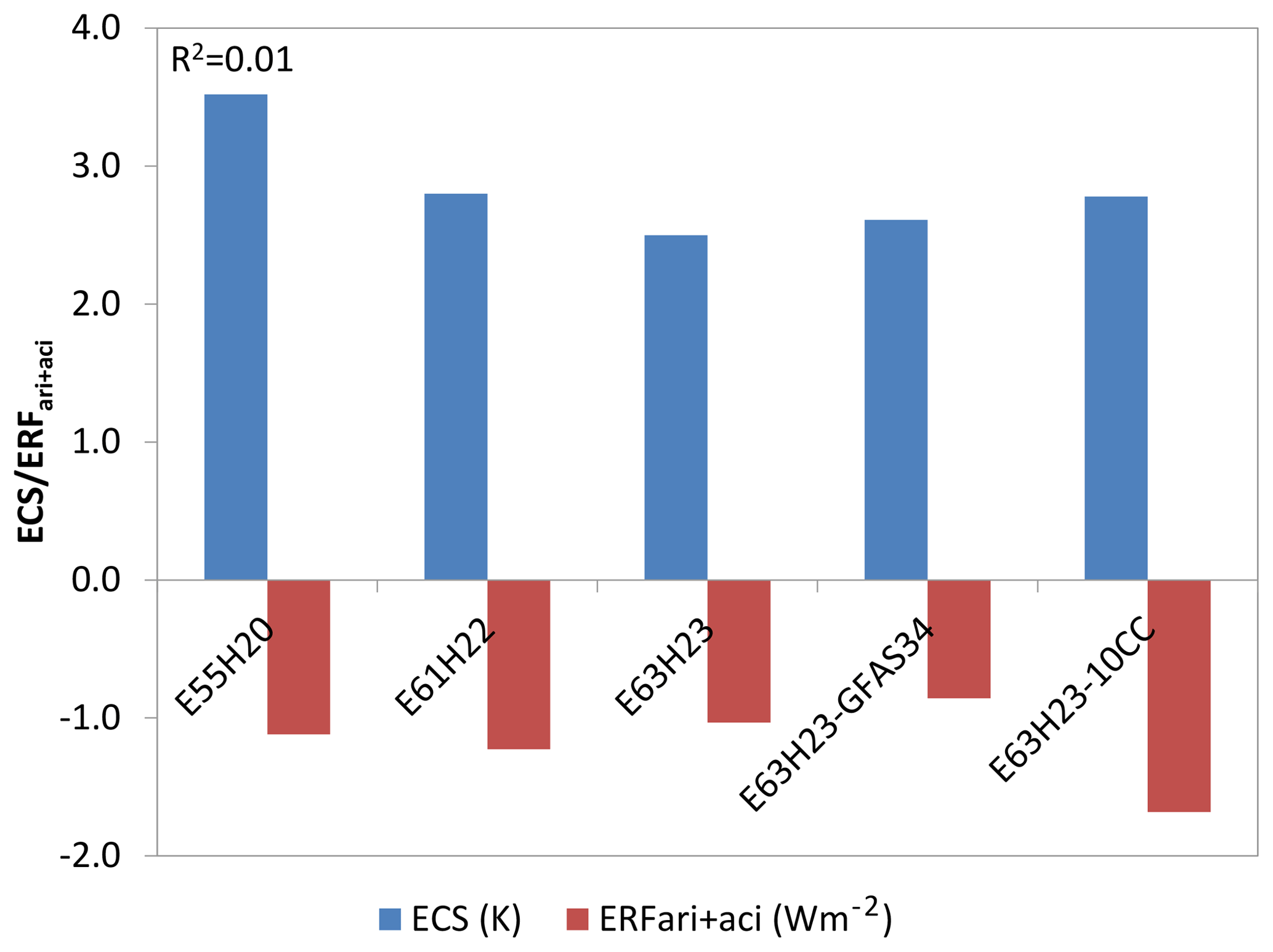
Figure 13Global mean ERF_ari+aci and ECS of E55H20, E61H22, E63H23, E63H23-GFAS34, and E63H23-10CC. The coefficient of determination between ERF_ari+aci and ECS is also displayed.

Download

The largest differences between E61H22 and E63H23 in terms of ERF_ari+aci are therefore due to a more realistic simulation of cloud water, the removal of a bug in ICNC, the new activation scheme, and the new sea salt emission parameterization in E63H23, whereas for ECS they are due to a more realistic simulation of cloud water and to model tuning.

3.6 Impact of changes and improvements in E63H23

The liquid phase of clouds is better represented in E63H23 than in the previous model versions because the low bias in cloud cover in the subtropics is reduced and the zonal distribution of LWP agrees with observations. This also leads to a better agreement of the SW CRE with observations in E63H23. Important reasons for these improvements are the change in the fractional cloud cover scheme for marine stratocumulus clouds, the removal of an inconsistency that had led to either 0 or 1 cloud cover in ECHAM6.3, and subsequent changes in model tuning (Mauritsen et al., 2019). Furthermore E63H23 uses the Abdul-Razzak and Ghan (2000) activation scheme and the Long et al. (2011) sea salt emission parameterization (temperature dependent; Sofiev et al., 2011), which leads to higher CDNCs when LWP is large. The Abdul-Razzak and Ghan (2000) activation scheme is more physically realistic than the empirical Lin and Leaitch (1997) activation scheme used in the previous model versions as it is Köhler theory based and therefore takes into account the size of the aerosol particles and their chemical composition. Although the Abdul-Razzak and Ghan (2000) activation scheme has limitations under certain conditions (the assumption that the aerosol particles are in equilibrium with its environment is not valid in all conditions; Phinney et al., 2003) and does not account for preexisting cloud droplets during cloud droplet activation (Barahona et al., 2010), it certainly helps to improve the representation of cloud droplets in E63H23. The performance of the new Long et al. (2011) (temperature dependent; Sofiev et al., 2011) and the old Guelle et al. (2001) sea salt parameterizations in E63H23 was analyzed by Tegen et al. (2019). The new temperature dependence leads to increased sea salt emissions where the sea surface temperature is warmer than 20 ^∘C and a decrease at colder temperatures. The new sea salt parameterization performs better, in particular with respect to number concentrations, than the previous sea salt parameterization compared to measurements on research cruises and at research stations. This is another indication that CDNCs are more realistic in E63H23 than in the previous model versions. The higher CDNCs in E63H23 allowed us to increase the tuning parameter for the autoconversion of cloud droplets to rain. Together these changes led to a better representation of the liquid phase of clouds in E63H23 and to a reduction of the SW component of ERF_ari+aci in E63H23 compared to E61H22 (because CCN concentrations from natural background aerosol are higher in E63H23).

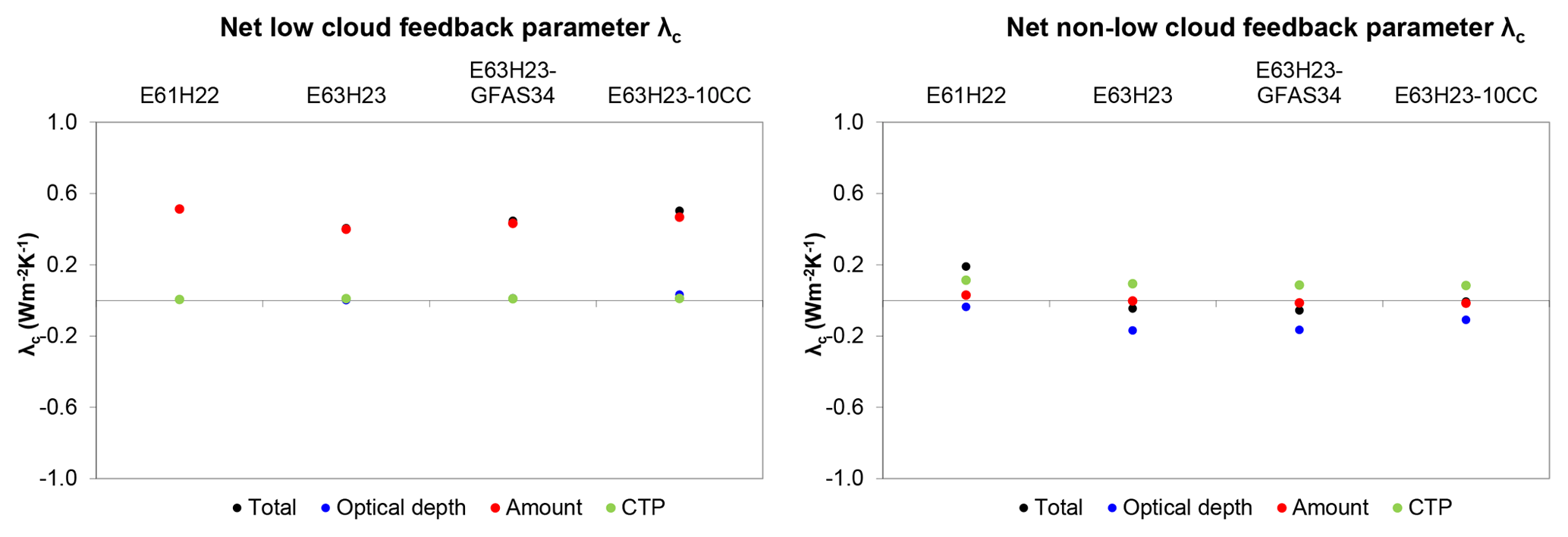
Figure 14Components of the net global mean cloud feedback parameter of E61H22 and E63H23 for low (cloud-top pressure (CTP) >680 hPa) and non-low (CTP <680 hPa) clouds.

Download

Also the ice phase of clouds has improved in E63H23 compared to previous model versions. The low bias in IWP is reduced in E63H23 and the global mean vertical IWC is within the observational range (Fig. 7). This is because the Seifert and Beheng (2006) sticking efficiency used in E63H23 leads to a less efficient removal of ice crystals by snow. A subsequent reduction in the tuning parameter for stratiform snow formation by aggregation further increases IWP in E63H23. Only a few laboratory studies for sticking efficiency have been conducted, and even fewer theories for sticking efficiency have been developed (Phillips et al., 2015). We find that the simple formulation of Seifert and Beheng (2006) for sticking efficiency for the accretion of ice crystals by snow improves the simulation of cloud ice in E63H23. Furthermore, the altitude of the global mean maximum IWC agrees well with observations in E63H23, whereas in E61H22 and E55H20 it is at higher altitudes than observed. This can be explained by the changes in ICNC described in Sect. 2.1.5, such as the use of a consistent ice crystal shape (hexagonal plates), removal of an ICNC bug, or the changed treatment of detrained ice crystals. The subsequent changes in precipitation formation and ice crystal sedimentation can then lead to a different vertical distribution of cloud ice. In E61H22 the global ICNC burden is considerably higher than in the other two model versions because of an inconsistency between cloud droplet activation, condensation, vertical transport of CDNC, and homogeneous freezing of cloud droplets in cirrus clouds, which led to homogeneous freezing of aerosol particles even when the water vapor pressure was too low for homogeneous nucleation. The higher ICNCs are also responsible for the LW component of ERF_ari+aci in E61H22 being more than twice as large as in the other two model versions. The good agreement of the global mean vertical distribution of IWC and LW CRE with observations in E63H23 is an indication that ICNC and the size of ice crystals are closer to reality in E63H23 than in the previous model versions. In a future version of the model we want to also include the competition for water vapor between homogeneous freezing of solution droplets, heterogeneous freezing of ice-nucleating particles, and preexisting ice crystals in cirrus cloud formation as has been done by Kuebbeler et al. (2014) and Gasparini et al. (2018), which should further improve the simulation of ICNC.

While the global mean values of RF_ari are quite similar between E63H23 and the previous model versions, there are regional differences. These are caused by the removal of inconsistencies in the model code and for E63H23 also by the new emission parameterization for mineral dust, which uses new satellite-based data for dust sources; this increases the confidence in the simulation of RF_ari in E63H23.

The weaker ECS in E63H23 compared to E61H22 can be linked to changes in cloud feedbacks. There are indications for a stronger cloud phase feedback in non-low clouds due to increased CDNC and changes in cloud water in E63H23. A stronger (cooling) cloud phase feedback will lead to less warming in the future. Similarly, the less positive cloud amount feedback of low clouds (related to model tuning in ECHAM6.3) in E63H23 contributes to the weaker ECS in E63H23 compared to E61H22.

The changes and improvements in E63H23 (including changes in the base model version ECHAM6.3) have therefore not only improved the representation of clouds in E63H23 compared to previous model versions, but they have also had an impact on ERF_ari+aci and ECS, decreasing both.