the Creative Commons Attribution 4.0 License.
the Creative Commons Attribution 4.0 License.
 | 27 Aug 2019
On the discretization of the ice thickness distribution in the NEMO3.6-LIM3 global ocean–sea ice model
François Massonnet
Antoine Barthélemy
Koffi Worou
Thierry Fichefet
Martin Vancoppenolle
Clément Rousset
Eduardo Moreno-Chamarro
The ice thickness distribution (ITD) is one of the core constituents of modern sea ice models. The ITD accounts for the unresolved spatial variability of sea ice thickness within each model grid cell. While there is a general consensus on the added physical realism brought by the ITD, how to discretize it remains an open question. Here, we use the ocean–sea ice general circulation model, Nucleus for European Modelling of the Ocean (NEMO) version 3.6 and Louvain-la-Neuve sea Ice Model (LIM) version 3 (NEMO3.6-LIM3), forced by atmospheric reanalyses to test how the ITD discretization (number of ice thickness categories, positions of the category boundaries) impacts the simulated mean Arctic and Antarctic sea ice states. We find that winter ice volumes in both hemispheres increase with the number of categories and attribute that increase to a net enhancement of basal ice growth rates. The range of simulated mean winter volumes in the various experiments amounts to ∼30 % and ∼10 % of the reference values (run with five categories) in the Arctic and Antarctic, respectively. This suggests that the way the ITD is discretized has a significant influence on the model mean state, all other things being equal. We also find that the existence of a thick category with lower bounds at ∼4 and ∼2 m for the Arctic and Antarctic, respectively, is a prerequisite for allowing the storage of deformed ice and therefore for fostering thermodynamic growth in thinner categories. Our analysis finally suggests that increasing the resolution of the ITD without changing the lower limit of the upper category results in small but not negligible variations of ice volume and extent. Our study proposes for the first time a bi-polar process-based explanation of the origin of mean sea ice state changes when the ITD discretization is modified. The sensitivity experiments conducted in this study, based on one model, emphasize that the choice of category positions, especially of thickest categories, has a primary influence on the simulated mean sea ice states while the number of categories and resolution have only a secondary influence. It is also found that the current default discretization of the NEMO3.6-LIM3 model is sufficient for large-scale present-day climate applications. In all cases, the role of the ITD discretization on the simulated mean sea ice state has to be appreciated relative to other influences (parameter uncertainty, forcing uncertainty, internal climate variability).


Sea ice forms a very heterogeneous medium at the surface of polar oceans. Open water, thin new ice, undeformed ice floes and thick pressure ridges may coexist on scales as small as a few meters (Thorndike et al., 1975; Williams et al., 2014). Several ocean–ice–atmosphere interaction processes are influenced by this small-scale heterogeneity. To quote only three, the ice growth rate critically depends on the local thickness (Maykut, 1982), the albedo of a given region is largely dependent on the presence of open water and thin ice (Maykut and McPhee, 1995; Holland et al., 2006a), and the areal extent of melt ponds depends on the local topography of sea ice (Eicken, 2002).
Sea ice models as components of climate models are primary tools to characterize climate variability at high latitudes (Holland et al., 2008), to diagnose the existence and the role of feedbacks (Goosse et al., 2018) and to estimate projected changes under various emission scenarios (Massonnet et al., 2012). They are also increasingly used to generate predictions from operational (Rabatel et al., 2018) to seasonal (Hamilton and Stroeve, 2016) timescales. The spatial resolution of sea ice models typically ranges from values as coarse as for paleoclimate studies to 1 km for short-range forecasting. As such, the high heterogeneity in sea ice thickness and therefore the complex nature of related physical processes cannot explicitly be modeled even in highest resolution configurations. The subgrid-scale variability of ice properties is often taken into account through the use of an ice thickness distribution (ITD). The ITD theory, as first introduced by Thorndike et al. (1975), aims at describing the time evolution of the statistical distribution of ice thickness in a given region under the action of thermodynamic growth and melt, advection by winds and currents, and mechanical redistribution by ridging, rafting and lead opening. In practice, the thickness distribution is discretized into a fixed number of categories. A compromise must be made, when choosing this number, between an accurate physical representation of the ITD and a containment of the computational costs.
The benefits of including an ITD for polar climate modeling have been addressed and recognized in numerous previous studies (e.g., Bitz et al., 2001; Holland et al., 2006b; Massonnet et al., 2011; Uotila et al., 2017; Ungermann et al., 2017). Pilot studies have attempted to determine the minimum number of categories necessary to resolve the seasonal cycle of climatically important variables. Using a Lagrangian formulation of the ITD, Bitz et al. (2001) concluded that five categories are sufficient to obtain the convergence of the Arctic sea ice extent and heat and freshwater fluxes, but that the volume is dependent on the details of the discretization for ice below 2 m thick. Similarly, Lipscomb (2001) suggested that five to seven categories, with higher resolution for thinner ice, are sufficient. Hunke (2014) rather stressed the importance of thick ice categories for proper modeling of Arctic sea ice volume. In particular, her results showed that simulations of Arctic ice volume require more than five categories, with a few of them above 2 m. Lately, Ungermann et al. (2017) demonstrated that the mean ice thickness in the Arctic increases with the number of categories used in the ITD and found that the better-resolved solution does not lead to the better model–data fit. Since simulations were tuned by minimizing cost functions, they did not investigate the physical processes explaining the model behaviors.
In this targeted study, we aim at assessing the response of a state-of-the-art coupled ocean–sea ice model, Nucleus for European Modelling of the Ocean (NEMO) version 3.6 and Louvain-la-Neuve sea Ice Model (LIM) version 3 (NEMO3.6-LIM3), to changes in the ITD discretization. From this model assessment, we wish to provide recommendations to the NEMO community (and more largely to users of large-scale sea ice models) regarding the number of thickness categories and the position of their boundaries, based on a physical understanding of the mechanisms at play. To our knowledge, all studies on the ITD but one (Holland et al., 2006b) focused on Arctic sea ice, so we wish to present a systematic assessment of the role of the ITD for sea ice in the Southern Hemisphere too. As we will see, the sensitivity of sea ice to the ITD discretization is generally less pronounced in that hemisphere than in the Northern Hemisphere. However, this might be an interesting indication of what will happen in the future in the Arctic Ocean, as its sea ice cover will become more seasonal in the near future (e.g., Massonnet et al., 2012). Finally, our objective is to understand the processes driving the model response to changes in the ITD discretization, a question that has not been explored in depth and that could be relevant for sea ice model developers beyond the NEMO-LIM community. To this end, we analyze ice volume tendency terms diagnosed in the model in order to separate thermodynamic contributions from dynamic ones but also surface from bottom ones. We focus our analysis on the response of the model climatology rather than on the long-term trends and interannual variability (which will be analyzed in a companion study).
This paper is organized as follows. The ocean–sea ice model (NEMO3.6-LIM3), its configuration and the series of sensitivity experiments are described in Sect. 2. The results are presented and discussed in Sect. 3. Conclusions and recommendations are finally drawn in Sect. 4. Note that all results and figures presented in this article can be reproduced bit-wise thanks to the archiving of the data and scripts on publicly available repositories (see “Code and data availability” at the end of the paper).
2.1 Ocean–sea ice model (NEMO3.6-LIM3)
This study is conducted using the dynamic–thermodynamic sea ice model LIM3.6 (Louvain-la-Neuve sea Ice Model; Rousset et al., 2015). It is coupled to a finite-difference, hydrostatic, free-surface, primitive-equation ocean model within version 3.6 of the NEMO framework (Nucleus for European Modelling of the Ocean; Madec, 2008). LIM includes an ITD, which is described in more details in the next section, energy conserving thermodynamics (Bitz and Lipscomb, 1999), a time-dependent salinity profile (Vancoppenolle et al., 2009a) and an elastic–viscous–plastic rheology formulated on a C grid to model the ice dynamics (Bouillon et al., 2013).
2.2 Ice thickness distribution
One of the key features of LIM is the ITD that is used to represent the subgrid-scale distribution of sea ice thickness, enthalpy and salinity (Thorndike et al., 1975). The probability density function for thickness h, , evolves according to the following equation:
The first term of the right-hand side is the convergence of the horizontal flux of g with u the ice velocity. In the second term, f is the thermodynamic growth rate. The third term, ψ, is the mechanical redistribution. The way this term is modeled is somewhat specific to LIM: it includes ridging and lead opening terms (as in other models) but also a rafting term (Vancoppenolle et al., 2009b). Another specificity of LIM is that newly formed ridges have a prescribed 30 % porosity.
The numerical formulation of the ITD in the model follows Lipscomb (2001). The thickness distribution is discretized into a fixed number of categories. Sea ice in each category occupies a varying areal fraction of the grid cell. Ice thickness in each category is constrained to remain between user-prescribed boundaries. Ice growth and melt induce transfers of ice volume and area between categories, which is dealt with the linear remapping scheme of Lipscomb (2001). This scheme combines the advantages of being computationally inexpensive and only weakly diffusive.
In the current version of LIM, the ITD is discretized by default by using a fitting function that places the category boundaries between 0 and , with the expected mean ice thickness over the domain. A greater resolution is placed for thin ice (Rousset et al., 2015). More specifically, the lower and upper limits for ice thickness in category are f(i−1) and f(i) with
where N is the number of categories, refers to the category index and α=0.05. The upper limit of the last category is always reset from to 99.0 m, in order to allow hosting very thick ice.
2.3 Model configuration
The configuration of NEMO3.6-LIM3 is almost identical to the one used in Barthélemy et al. (2017), where the reader may find the details that are not recalled here. The revision 6631 of the branch 2015/nemo_v3_6_STABLE of the NEMO SVN repository (https://forge.ipsl.jussieu.fr/nemo/svn/NEMO/releases/release-3.6/, last access: 19 August 2019) is used. The ocean and sea ice models are run on the global eORCA1 grid, which has a nominal resolution of 1∘ in the zonal direction. In the ocean, a partial step z coordinate with 75 levels is used along the vertical. The layer thickness increases non-uniformly from 1 m at the surface to 10 m at 100 m depth and reaches 200 m at the bottom. To avoid spurious model drift, a weak restoring towards the World Ocean Atlas 2013 surface salinity climatology (Zweng et al., 2013) is applied, with strength 167 mm d−1 (i.e., a relaxation timescale of 10 months for a 50 m deep oceanic mixed layer). In order to avoid adversely altering ocean–ice interactions, this restoring is damped under sea ice (multiplied by 1 minus sea ice concentration), i.e., where the observations are less reliable.
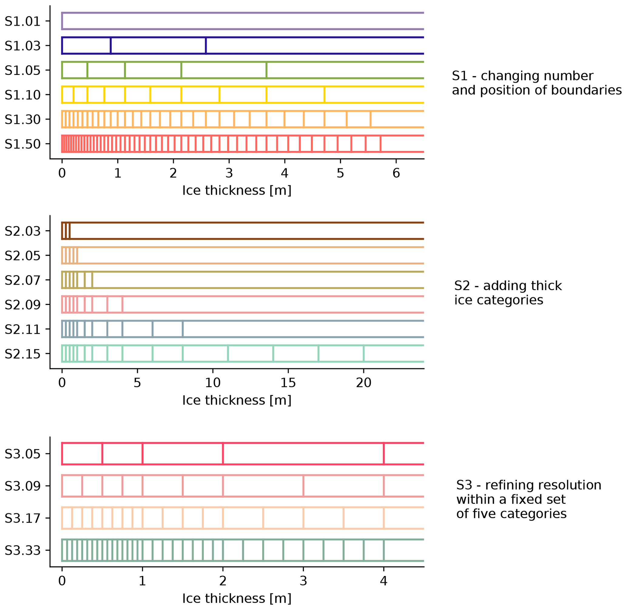
Figure 1Ice thickness category boundaries in the three sets of sensitivity experiments. The upper boundary of the last category is always set to 99.0 m. Note that the ice thickness scale is different in the three panels. Because the ITD discretization in the third set of experiments (S3) branches from experiment S2.09 of the second set, that experiment is repeated in the list but labeled as S3.09.
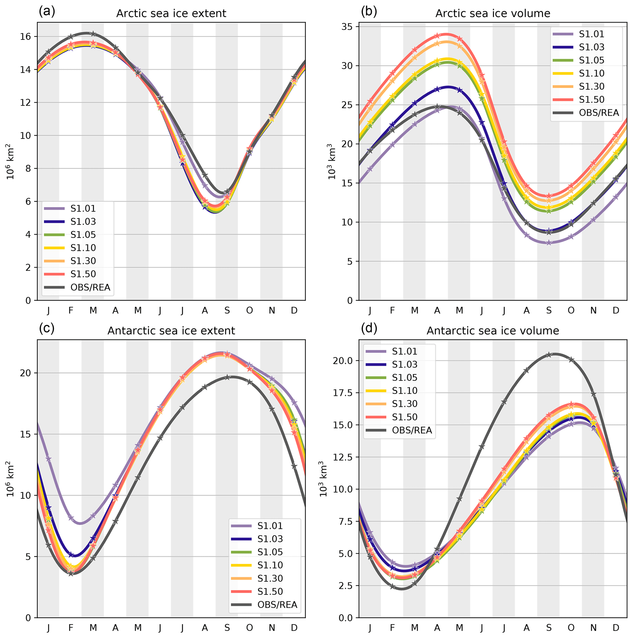
Figure 2Mean seasonal cycles of Arctic (a, b) and Antarctic (c, d) sea ice extents (a, c) and volumes (b, d), over 1995–2014, in the first set of sensitivity experiments. Ice extents derived from the Ocean and Sea Ice Satellite Application Facility (OSISAF) sea ice concentration observational product (OSI-409a; EUMETSAT, 2015) are also shown, as well as Arctic and Antarctic ice volumes derived from the Pan-Arctic Ice Ocean Modeling and Assimilation System (PIOMAS) and Global Ice Ocean Modeling and Assimilation System (GIOMAS) reanalyses, respectively (Schweiger et al., 2011; Zhang and Rothrock, 2003). The stars show the monthly data and the curves are cubic interpolations between the data points.
The atmospheric forcing is provided by the DRAKKAR Forcing Set version 5.2 (DFS5.2; Brodeau et al., 2010; Dussin et al., 2016). This global forcing set is derived from the ERA-Interim reanalysis over 1979–2015 and from ERA-40 for the period 1958–1978. It has a spatial resolution close to 0.7∘, or 80 km, and is utilized within the CORE forcing formulation of NEMO, which uses bulk formulas developed by Large and Yeager (2004). Continental freshwater inputs consist of river runoff rates from the climatological dataset of Dai and Trenberth (2002) north of 60∘ S, of prescribed meltwater fluxes from ice shelves along the coastline of Antarctica (Depoorter et al., 2013) and of climatological freshwater fluxes from iceberg melt at the surface of the Southern Ocean (Merino et al., 2016). The sole difference compared to Barthélemy et al. (2017)'s setup is the shorter integration time (1979–2015 instead of 1958–2015) due to the computational cost of the multiple sensitivity experiments. Simulations are only weakly impacted by the length of integrations. A comparison of the reference simulation labeled S1.05 (see below) with the corresponding experiment in the aforementioned study indicates that the interannual variability of hemispheric ice volumes is the only sea ice index showing a weak sensitivity to the start date, while other ones are not affected (not shown). The ocean is initialized at rest with temperature and salinity fields from the World Ocean Atlas 2013 (Locarnini et al., 2013; Zweng et al., 2013) and we analyze the last 20 years of the simulations (1995–2014).
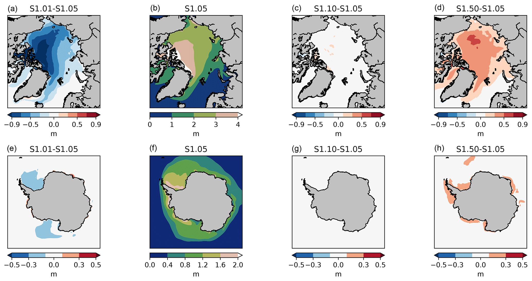
Figure 3Effective sea ice thickness (grid-cell ice volume divided by grid-cell area) in the Arctic in March (top) and in the Antarctic in September (bottom), averaged over 1995–2014. Experiment S1.05 and differences with selected experiments of the first set are shown.
2.4 Sensitivity experiments
An ITD discretization features two characteristics: the number of categories used and the position of category boundaries. By default, the LIM automatically sets the position of category boundaries for a given number of categories, according to Eq. (2). However, this choice can be overridden by the user, in order to explore specific discretizations.
We ran three successive sets of sensitivity experiments. In the first set, labeled S1, the default ITD discretization of LIM is used and both the number and positions of category boundaries change according to Eq. (2) for a number of 1, 3, 5, 10, 30 and 50 categories. The value for is set to 2.0 m and represents a tradeoff between gross estimates of Antarctic and Arctic basin-wide average thickness (∼1.0 and 3.0 m, respectively). The category boundaries are displayed in the top panel of Fig. 1.
The results derived from this first set of experiments can potentially be useful for users of the model but not necessarily for understanding the physical processes driving the model response. Indeed, in S1, both the position and the resolution of the thickness categories vary from one experiment to the next; it is thus impossible to disentangle one effect from the other. Therefore, in a second set of experiments, labeled S2, we bypass the default formulation of LIM and successively append new thickness categories without changing the existing category boundaries (Fig. 1, middle panel). This set of experiments allows testing the influence of thick ice categories, as Hunke (2014) suggested this aspect to be potentially important. In that set of experiments, the resolution of the ITD is unchanged and we can test the specific role of the category positions on the simulated mean sea ice state.
Finally, in order to test the influence of the number of ice categories, independently of their position, we run a third set of sensitivity experiments (S3), in which the lower boundary of the thickest category is locked to 4.0 m as in experiment S2.09, and the ITD is coarsened/refined by merging/splitting the existing categories (Fig. 1, bottom panel). The upper limit of 4.0 m corresponds to the maximum thickness that thermodynamic ice growth can sustain in the Arctic (Maykut and Untersteiner, 1971) and allows therefore the thickest category to host the deformed ice produced by the model.
3.1 Influence of the number of categories in the default formulation (S1 experiments)
Seasonal cycles of Arctic and Antarctic sea ice extents and volumes are presented in Fig. 2. Following the usual conventions, sea ice extent is defined as the sum of all oceanic grid-cell areas that contain at least 15 % of ice concentration, while sea ice volume is defined as the sum of individual grid-cell volumes. The main consequence of using a larger number of ice thickness categories is to increase the ice volume in winter. In the Arctic, the increase persists during the whole seasonal cycle, even though it becomes smaller in summer. To position the volume produced by our model, a comparison is made with the Pan-Arctic Ice Ocean Modeling and Assimilation System (PIOMAS) reanalysis (Schweiger et al., 2011). The model produces higher volume than the PIOMAS reanalysis for simulations with more than three categories. In the Antarctic, the increase is limited to the ice growing season, while the rest of the year features a decrease in volume when using only few categories (S1.01 and S1.03), which is due to an excessive sea ice extent in summer (discussed later). In either hemisphere, the annual maximum of ice volume does not converge to an asymptotic value when increasing the number of categories. The possible origins of this lack of convergence will be discussed in the next section.
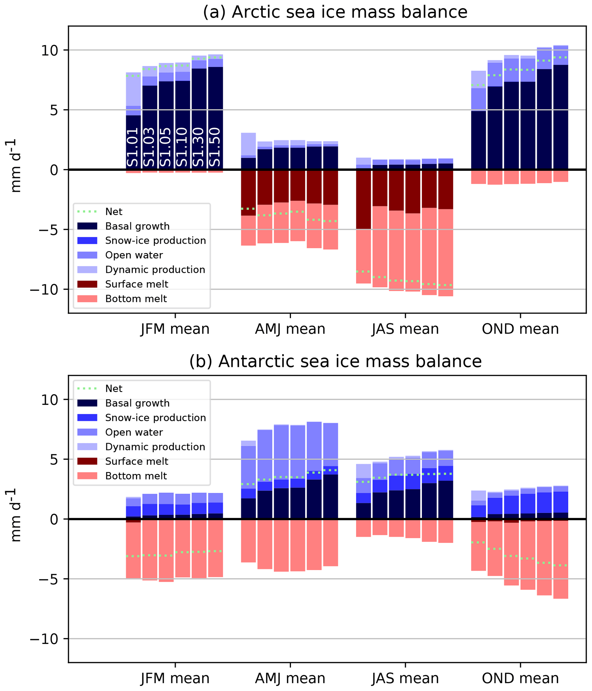
Figure 4Contributions to the seasonal mass balance of Arctic (a) and Antarctic (b) sea ice as simulated in the first set of sensitivity experiments (S1) (varying number of categories with the default LIM3 ITD discretization), averaged over the areas depicted in Fig. A1. Blue colors refer to processes that contribute to positive ice volume changes, while red colors indicate processes implying negative ice volume changes. The name of the experiments is indicated in the upper panel for the January–February–March season.
3.1.1 Response of sea ice thickness
The impact of changing the number of categories on the spatial distribution of ice thickness is shown in Fig. 3. Compared to experiment S1.05, using only one category reduces the ice thickness mainly in the thick ice areas, by up to 1 m north of the Canadian Arctic Archipelago and the Canadian basin in the Arctic, and by around 0.2 m in the Ross and Weddell seas in the Antarctic. By contrast, increasing the number of categories leads to a more uniform thickening of the ice, by up to 0.5 m (0.2 m) for S1.50 in the Arctic (Antarctic).
The origin of a thickness increase with the number of ice thickness categories can be explored with the tendency diagnostics provided in LIM. Indeed, variations in state variables, including volume in each category and therefore the aggregate volume, can be attributed to various physical processes accounted for in the model such as open-water ice formation, bottom growth, snow-ice production and dynamic production (i.e., ice formed due to refreezing of seawater after entrapment into porous ridges) but also bottom melt and surface melt.
The increase in sea ice thickness is mainly due to an enhancement of thermodynamic basal growth rates in fall and winter (Fig. 4). Our hypothesis is that, for the same grid-cell average thickness, a better-resolved ITD results in larger basal ice growth rates due to the inverse relationship between conductive heat fluxes and sea ice thickness. To illustrate this point, let us consider two counterfactual configurations A and B, with the same grid-cell average ice thickness but different ITDs. In A, a uniform 2 m thick slab of ice covers 100 % of the grid cell, while in B 50 % of the grid cell is covered by a 1 m thick slab of ice and the other 50 % by a 3 m thick slab of ice. All other things being equal (surface and bottom ice temperatures, snow, ice conductivity, ocean–ice heat flux), the heat conduction flux will be proportional to 1∕2 W m−2 in A as per Fourier's law of conduction. By contrast, the heat conduction flux will be proportional to 1 and 1∕3 W m−2 on each half of the grid cell in B, giving an average of 2∕3 W m−2. The basal ice growth, resulting from the imbalance between ocean–ice heat flux and the heat conduction flux, will therefore be higher in B.
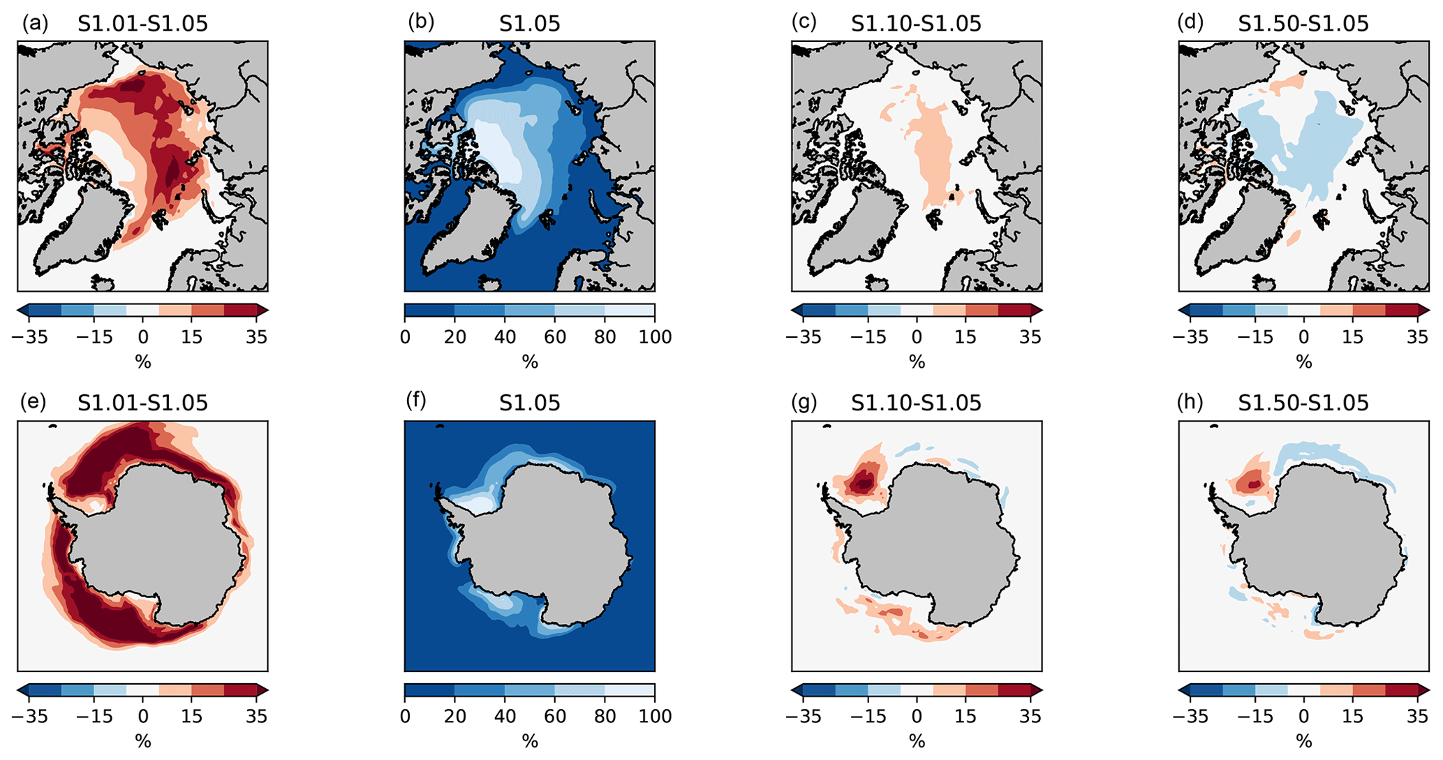
Figure 5Sea ice concentration in the Arctic in August (top) and in the Antarctic in February (bottom), averaged over 1995–2014. Experiment S1.05 and differences with selected experiments of the first set are shown.
The diagnosed sea ice mass balance analysis of Fig. 4 also shows that, in the Arctic, the run with one thickness category compensates the deficit of basal ice growth (relative to multi-category runs) by enhanced dynamic production during fall and winter (October to March). We can understand this finding as follows. First, the deficit of ice growth leads to a thinner ice pack. However, in the model, compressive ice strength is a function of the grid-cell average thickness H and the concentration A:
where kN m−2 and C=20 are two empirical constants. In all simulations, A∼1 in winter due to the thermal constraint imposed by the atmospheric forcing. Small values of H in the one-category simulation lead to less resistance of ice to compression and hence enhanced mechanical redistribution, which fosters dynamic growth.
What is the origin of non-convergence of sea ice volumes noticed in Fig. 2? Based on the mass balance analysis, the non-convergence is primarily due to a non-convergence in basal growth rates (Fig. 4). However, in an idealized configuration with no snow and without ice dynamics, growth rates reach 95 % of the asymptotic value when five categories or more are used (Fig. 6). Thus, the non-convergence has to be the consequence of an interplay between the dynamic and thermodynamic processes: ridging or rafting transfers thin ice to thicker categories, allowing more ice production by thermodynamic growth. It is not possible to produce deeper analyses at this stage as the ice mass balance terms are only available at the grid-cell level, not at the ice thickness category level. It is also unclear if the non-convergence is the consequence of our experimental setup in which the atmospheric forcing is prescribed – offering no possibility for negative feedbacks to operate or at least not as strongly as they might do in a coupled model. We will soon be testing this hypothesis with a coupled model.

Figure 6(a) A supposed ice thickness distribution in a model grid cell (red; log-normal distribution with mean 3 m and standard deviation 2 m) and its discretization in five categories following the default formulation of LIM3 (grey bars). (b) Average basal growth rates for categories. For each category, the basal growth rate was computed assuming sea ice thickness equal to the category mean (hi with , where N is the number of categories), assuming no snow, an atmosphere–ocean temperature difference of ΔT=30 K, sea ice conductivity of k=2 W mK−1, latent heat of fusion of Lf=334 000 J kg−1 and sea ice density of ρi=917 kg m−3. The growth rates were then averaged over categories, taking into account the relative area of each category: , with dhi the width of category i.
3.1.2 Response of sea ice concentration
In winter, the sea ice concentration within the ice pack is close to 100 % in all simulations, and the total ice extent shows no sensitivity to the ITD discretization (Fig. 2). This was expected, since the same prescribed atmospheric forcing is used throughout all sensitivity experiments: in all cases, the ice edge follows to a first approximation the 0 ∘C isotherm of SST and of the near-surface air temperature field in the atmospheric forcing.
By contrast to the winter response, the summer response of sea ice concentration to the ITD discretization is noticeable, especially for the run with one category (Fig. 5). To understand these differences, we first recall that sea ice concentration at the end of the melting season is defined by three factors: the initial thickness (thick ice is less prone to melt away during summer, Goosse et al., 2009), the strength of the ice-albedo feedback and the history of atmospheric conditions (advection of warm air or moisture, anomalous radiative fluxes, advection of mechanical redistribution induced by winds). This latter factor cannot explain the differences seen in Fig. 5, since the same forcing is used in all experiments. As for the ice-albedo feedback, including ITD is known to enhance it: open-water formation is more active as sea ice thins (Bitz et al., 2001; Holland et al., 2006a; Massonnet et al., 2018). Higher sea ice concentrations in summer in S1.01 are suggestive of a weaker feedback in these experiments. The impact is strong enough to be visible on the mean seasonal cycles of ice extent (Fig. 2). By the same reasoning, the large number of thin categories in S1.50 is likely causing a stronger feedback, which explains the lower concentrations in August in the Arctic. However, (first factor) thicker ice is less prone to melt during summer. Since we have shown above that increasing the number of ITD categories also increases the ice thickness, this counteracts the effect related to the ice-albedo feedback. The competition between both effects results in a non-linear response of the summer sea ice concentration to changes in the number of thickness categories. This is why there is, at least for runs with more than one category, no obvious dependence of the mean summer sea ice concentration on the number of categories used in the ITD discretization in Fig. 5.
While the Arctic and Antarctic summer sea ice concentration responses for two or more categories appear to be complex for the reasons explained above, the run with one category displays a consistent increase in concentration (Fig. 5) and extent (Fig. 2) in both hemispheres. In one-category runs, it is not possible to melt thin ice as efficiently as in multi-category runs, since by definition there is no dedicated room for thin ice. Our hypothesis is that, in those runs, sea ice melt occurs mostly by thinning and not so much by lateral melting, thus leaving large ice-covered areas by the end of local summer.
3.2 Influence of thick ice categories (S2 experiments)
The aim of the second set of sensitivity experiments is to examine specifically the importance of thick ice categories in the ITD, without refining the discretization in the thin range (Fig. 1, middle panel). In this set, the sea ice volume is again the variable that is most impacted by the selected number of categories (Fig. 7). The Arctic ice volume increases monotonically with the addition of new thick categories until a threshold at ∼4 m is reached: adding categories beyond that threshold (experiments from S2.09 on) does not have an impact on the total volume. The Antarctic ice volume is less sensitive.
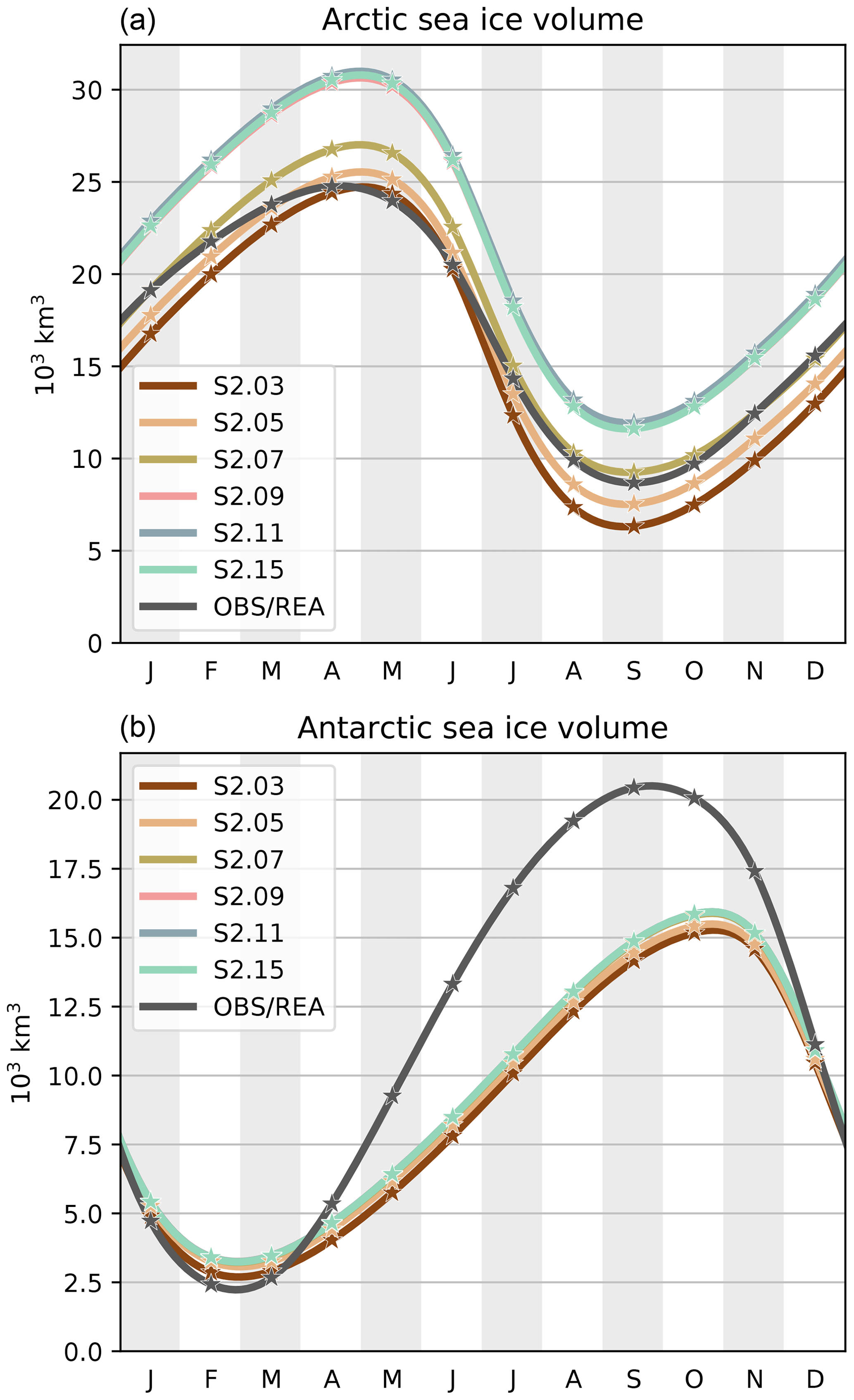
Figure 7Mean seasonal cycles of Arctic (a) and Antarctic (b) sea ice volumes, over 1995–2014, in the second set of sensitivity experiments. Also shown are the Arctic and Antarctic ice volumes derived from the PIOMAS and GIOMAS reanalyses, respectively (Schweiger et al., 2011; Zhang and Rothrock, 2003). The stars show the monthly data and the curves are cubic interpolations between the data points.

Figure 8Mean ice thickness distribution in the second set of sensitivity experiments. For each ice thickness category, the relative areal proportion of ice for that category was estimated from the Arctic (March, top) and Antarctic (September, bottom) 1995–2014 average sea ice concentration field restricted to the domain shown in Fig. A1. Thin vertical lines delimit the category boundaries. Note that, for the sake of readability, the spacing along the x axis is logarithmic. The upper bound of the last category is always set to 99.0 m and is not displayed.
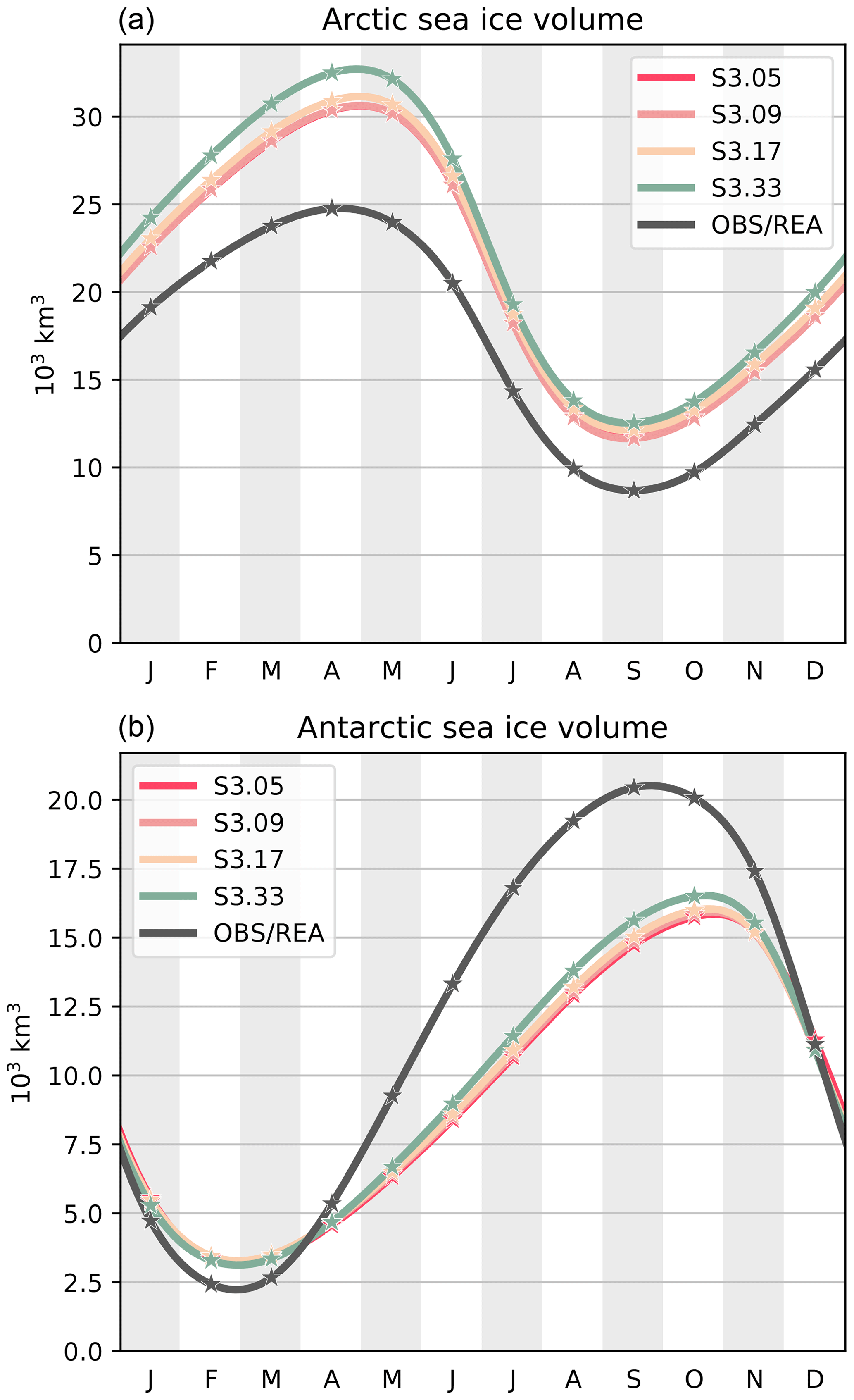
Figure 9Mean seasonal cycles of Arctic (a) and Antarctic (b) sea ice volumes, over 1995–2014, in the third set of sensitivity experiments. Also shown are the Arctic and Antarctic ice volumes derived from the PIOMAS and GIOMAS reanalyses, respectively (Schweiger et al., 2011; Zhang and Rothrock, 2003). The stars show the monthly data and the curves are cubic interpolations between the data points.
In order to understand the origin of this convergence of sea ice volume, we show in Fig. 8 the mean ITDs in March in the Arctic and in September in the Antarctic. March and September correspond to the hemispheric ice extent maxima and are 1 month ahead of the ice volume maxima. The volume gains essentially stop (from S2.09 and S2.07 on in the Northern Hemisphere and Southern Hemisphere, respectively) when there exist categories that can contain the very thick ice produced by ridging (around 10 m and above). When this is the case, the thickest ice occupies only a small fraction of the grid cells, leaving more room for thinner ice that can sustain non-negligible thermodynamic growth rates. Including additional thicker categories allows a more detailed representation of the ice cover but without effects on the growth rates and thereby on the total volumes. The threshold values of 4 m (Arctic) and 2 m (Antarctic) are no coincidence. Maykut and Untersteiner (1971) found that the equilibrium thickness of level ice would reach 3–4 m in standard Arctic conditions. In the Antarctic, a larger climatological snow depth and larger ocean–ice basal heat flux both contribute to a thinner level ice cover on average.
We also note that the Arctic sea ice volume is more sensitive than the Antarctic sea ice volume in the S2 set of experiments (Fig. 7). This is because, in the model, the proportion of Antarctic ice volume produced by deformation (and stored in the thickest categories) is low compared to the Arctic. Creating the categories to host that deformed ice thus has only a moderate effect in the Antarctic. An investigation of the ability of NEMO3.6-LIM3 to realistically simulate the volume of deformed ice is currently underway in another study. We conclude that setting the lower boundary of the thickest category at 4 and 2 m for the Arctic and Antarctic, respectively, is sufficient to allow convergence in simulated ice volumes, provided that the resolution of the ITD in the thin categories remains unchanged. These conclusions hold for present climate conditions and may have to be updated for other applications (e.g., paleoclimate simulations).
3.3 Influence of increasing resolution (S3 experiments)
In the previous set of experiments (S2), we have determined the minimal requirements for the position of the thick ice category in order to achieve convergence of ice volumes, without refining the ITD elsewhere. The final set of sensitivity experiments (S3) is designed to assess the specific role of the resolution of the ITD discretization in the thin range, without changing the upper bound (set to 4 m since we are using a global model). Starting from experiment S2.09 (renamed S3.09 in this third set of experiments), we coarsen and refine the ITD by merging or splitting category boundaries in two. Figure 9 shows the mean seasonal cycles of Arctic and Antarctic sea ice volumes. Increasing the resolution leads to higher sea ice volumes through enhanced bottom growth rates (Fig. A3), as explained in Sect. 3.1. However, the differences become significant in the Arctic only for S3.33, in which the ITD resolution is 4 times finer than in S3.09. Overall, these results suggest that refining the ITD resolution by adding more intermediate categories has a small but not negligible impact on the total simulated sea ice volume.
In line with the results of Sect. 3.2, we conclude that the position of the thickest category (S2 experiments) exerts a first-order control on the total sea ice volume by allowing the existence of thick and deformed ice, while the resolution of the ITD discretization in the thin range (S3 experiments) has a second-order effect on the total volume, by controlling the amount of thermodynamically grown ice.
The objective of this study was to examine the sensitivity of Arctic and Antarctic sea ice, as simulated by the global ocean–sea ice general circulation model (NEMO3.6-LIM3), to the discretization of the ITD. Indeed, previous studies using coupled (Bitz et al., 2001; Holland et al., 2006b) and uncoupled (Massonnet et al., 2011; Uotila et al., 2017; Ungermann et al., 2017; Hunke, 2014) models suggested the potential role of the ITD discretization on the simulate mean sea ice state. We aimed at understanding the physical processes behind the model responses. Our results have shown that increasing the number of categories leads to an increase of winter sea ice volumes, which persists in summer in the Arctic. In both hemispheres, the summer extents are sensitive to the number of categories only for fewer than five categories. Higher winter ice volumes are caused by higher thicknesses due to enhanced bottom growth, which is related to the ice thickness distribution discretization via the conductive heat flux through the ice. Our results also indicate that the inclusion of a very large number of ice thickness categories does not systematically improve the realism of the simulations against available observational references and reanalyses (Fig. 2). However, these sensitivity experiments have not been tuned (unlike the reference experiment). In addition, verification data are uncertain: for sea ice extent, variations among products can reach values as high as 1 million km2 (Meier and Stewart, 2018). The sea ice volume values provided for reference in our figures are even more uncertain, being estimated from reanalyses. No strict convergence of ice volumes is achieved with less than 10 categories and the following observations can be made. First, it is required to have categories with lower bounds around 4 and 2 m in the Arctic and the Antarctic, respectively. When this is not the case, the thick ice produced by ridging is blended with thinner ice, increasing its thickness, reducing the bottom growth and eventually decreasing the total ice volume. This confirms and explains the importance of thick ice categories already noted for the Northern Hemisphere by Hunke (2014). The existence of these thick categories is critical to host deformed ice and to let thin ice, which is subject to high basal growth rates in winter, occupy a sufficient fraction of the grid cells. Second, refining the ice thickness distribution discretization in the thin range (below 4 and 2 m for the Arctic and Antarctic, respectively) causes hemispheric ice volumes to keep growing, though a very large number of categories (at least 33) is necessary to detect a significant increase. We stress that, by design, our experimental protocol ignores possible feedbacks between the atmosphere and the ice–ocean system, which could enhance or damp the responses seen in our results.
One important criterion when choosing the ice thickness distribution discretization is the associated computing cost. Compared to a reference case with one category, computing time increases by 2 %–6 % when five categories are used, by 42 % when 17 categories are used and by 210 % when 50 categories are used (Fig. A4). However, as discussed above, the gains in terms of convergence of modeled sea ice volumes are weak for such a number of categories. Hence, using five categories, with sufficiently thick categories, appears to be an appropriate compromise for global experiments: the ice extent converges in both hemispheres, while a reasonable level of convergence is reached for ice volume. Simulations of the Southern Ocean sea ice may require fewer categories, while applications needing a very detailed representation of the thick Arctic sea ice should use a much finer ice thickness distribution discretization. Thus, for large-scale climate applications with NEMO3.6-LIM3, we recommend using the default ITD discretization (experiment S1.05).
It is finally important to place the results of the sensitivity tests conducted in this study in a broader context. Specifically, one should investigate how the sea ice volume and extent responses seen in this study compare to other influences. For instance, the net increase of km3 in annual mean Arctic sea ice volume, seen in Fig. 2 when changing from S1.05 to S1.50, lies in the 2–5×10³ km3 range of interannual variability noted by Olonscheck and Notz (2017), who analyzed the output from climate models participating in the fifth phase Coupled Model Intercomparison Project (CMIP5). The response is in addition much smaller than the range obtained in the sensitivity tests conducted by Urrego-Blanco et al. (2016) to various parameters in the CICE model. The response is also small compared to the range of sea ice volumes estimated by state-of-the-art sea ice reanalyses (Chevallier et al., 2016), which are supposed to be among the best constrained estimates on this quantity. In conclusion, choices related to the ITD discretization should always be put in the perspective of other competing influences, such as parameter tuning and background internal variability (Notz, 2015), the choice of atmospheric forcing (Barthélemy et al., 2017; Hunke, 2010) and the choice of observational references or reanalyses (Massonnet et al., 2018) used to evaluate the outcome of such sensitivity tests.
The source code of the model used and the source code of the scripts used to produce the figures and results of the paper are available at https://doi.org/10.5281/zenodo.3345604 (Massonnet et al., 2019). Model output is available upon request but can also be downloaded from the aforementioned URL.
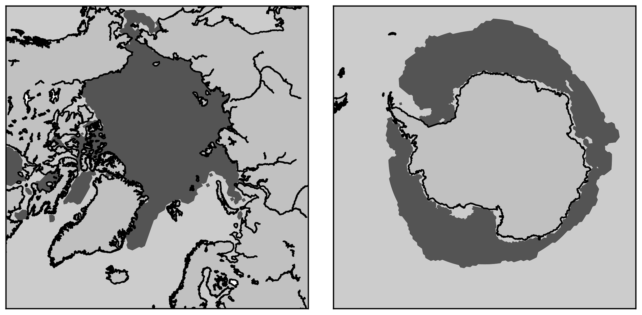
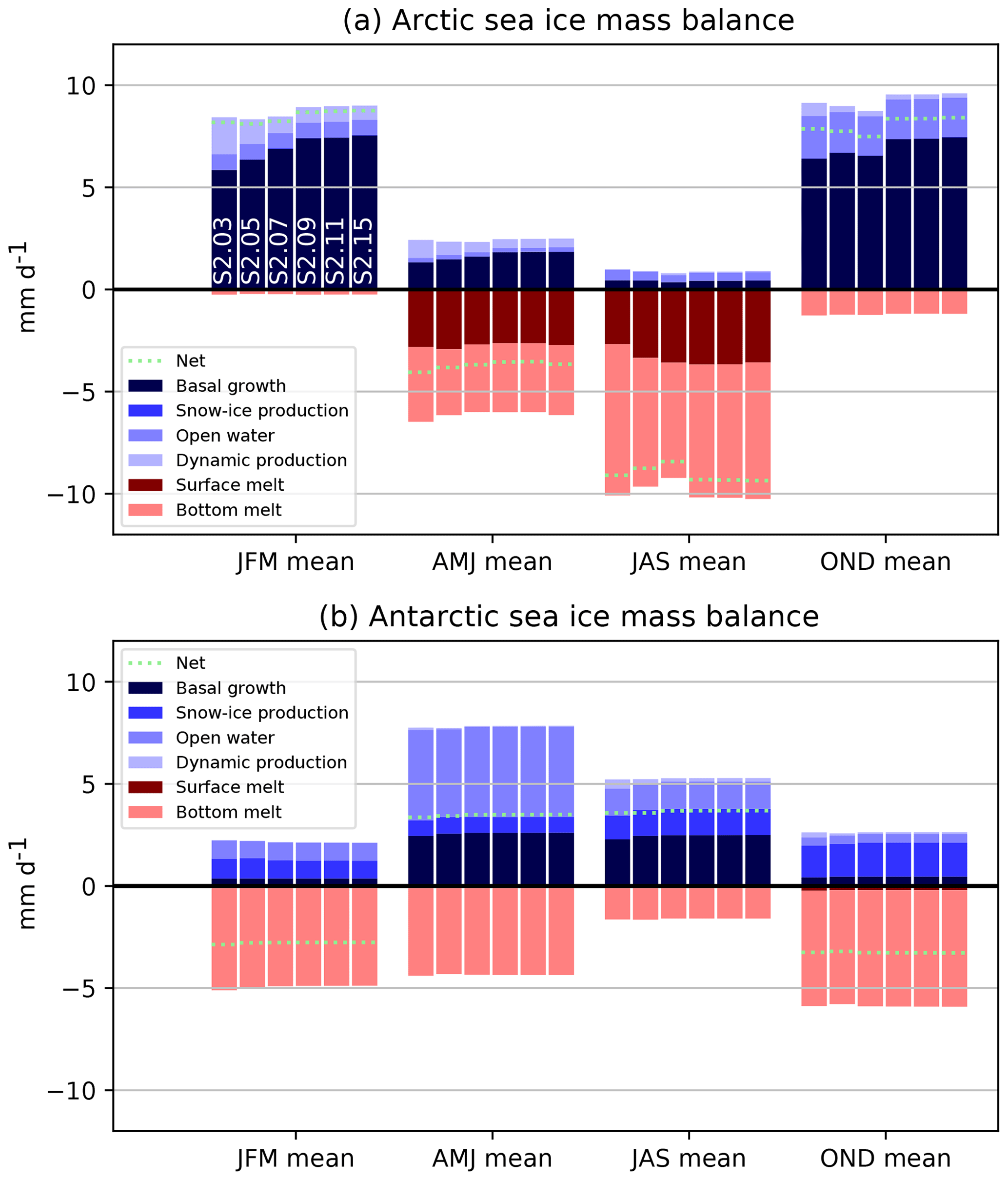
Figure A2Contributions to the seasonal mass balance of Arctic (a) and Antarctic (b) sea ice as simulated in the second set of sensitivity experiments (S2) (appending thick ice categories), averaged over the areas depicted in Fig. A1. Blue colors refer to processes that contribute to positive ice volume changes, while red colors indicate processes implying negative ice volume changes. The name of the experiments is indicated in the upper panel for the January–February–March season.

Figure A3Contributions to the seasonal mass balance of Arctic (a) and Antarctic (b) sea ice as simulated in the third set of sensitivity experiments (S3) (refining the ITD within a fixed set of categories), averaged over the areas depicted in Fig. A1. Blue colors refer to processes that contribute to positive ice volume changes, while red colors indicate processes implying negative ice volume changes. The name of the experiments is indicated in the upper panel for the January–February–March season.
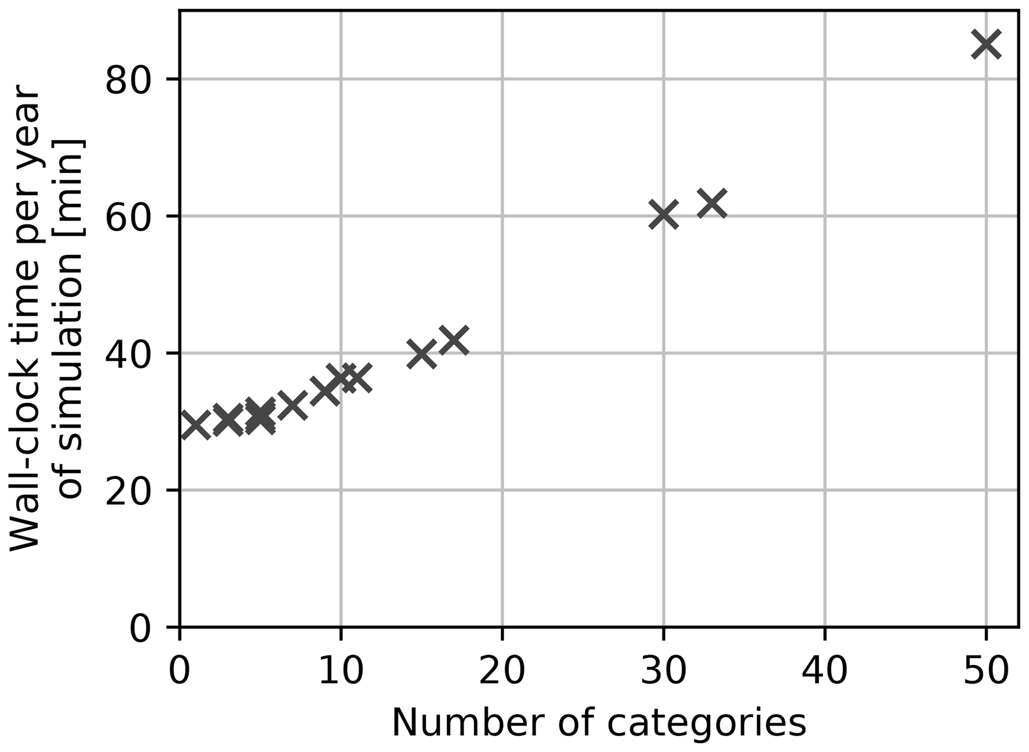
Figure A4Wall-clock time required for 1 year of simulation as a function of the number of ice thickness categories. The coupled ocean–sea ice model is run on 260 cores. The computing times indicated in this figure correspond to the average over the first 5 years of each simulation.
AB, TF, KW and FM designed the study. AB ran the experiments. AB and FM wrote the manuscript. All authors provided scientific input.
The authors declare that they have no conflict of interest.
Computational resources have been provided by the supercomputing facilities of the Université catholique de Louvain (CISM/UCL) and the Consortium des Equipements de Calcul Intensif en Fédération Wallonie Bruxelles (CECI) funded by the F.R.S.-FNRS under convention 2.5020.11. François Massonnet is a F.R.S.-FNRS Research Associate. The research leading to these results has received funding from the European Commission's Horizon 2020 APPLICATE (GA 727862) and PRIMAVERA (GA 641727) projects.
This research has been supported by the European Commission (APPLICATE (grant no. 727862) and PRIMAVERA (grant no. 641727)).
This paper was edited by Qiang Wang and reviewed by two anonymous referees.
Barthélemy, A., Goosse, H., Fichefet, T., and Lecomte, O.: On the sensitivity of Antarctic sea ice model biases to atmospheric forcing uncertainties, Clim. Dynam., 51, 1585–1603, https://doi.org/10.1007/s00382-017-3972-7, 2017. a, b, c
Bitz, C. M. and Lipscomb, W. H.: An energy-conserving thermodynamic model of sea ice, J. Geophys. Res., 104, 15669–15677, https://doi.org/10.1029/1999JC900100, 1999. a
Bitz, C. M., Holland, M. M., Weaver, A. J., and Eby, M.: Simulating the ice-thickness distribution in a coupled climate model, J. Geophys. Res., 106, 2441–2463, https://doi.org/10.1029/1999JC000113, 2001. a, b, c, d
Bouillon, S., Fichefet, T., Legat, V., and Madec, G.: The elastic-viscous-plastic method revisited, Ocean Modell., 71, 2–12, https://doi.org/10.1016/j.ocemod.2013.05.013, 2013. a
Brodeau, L., Barnier, B., Treguier, A.-M., Penduff, T., and Gulev, S.: An ERA40-based atmospheric forcing for global ocean circulation models, Ocean Modell., 31, 88–104, https://doi.org/10.1016/j.ocemod.2009.10.005, 2010. a
Chevallier, M., Smith, G. C., Dupont, F., Lemieux, J.-F., Forget, G., Fujii, Y., Hernandez, F., Msadek, R., Peterson, K. A., Storto, A., Toyoda, T., Valdivieso, M., Vernieres, G., Zuo, H., Balmaseda, M., Chang, Y.-S., Ferry, N., Garric, G., Haines, K., Keeley, S., Kovach, R. M., Kuragano, T., Masina, S., Tang, Y., Tsujino, H., and Wang, X.: Intercomparison of the Arctic sea ice cover in global ocean–sea ice reanalyses from the ORA-IP project, Clim. Dynam., SI, 1–30, https://doi.org/10.1007/s00382-016-2985-y, 2016. a
Dai, A. and Trenberth, K. E.: Estimates of Freshwater Discharge from Continents: Latitudinal and Seasonal Variations, J. Hydrometeor., 3, 660–687, https://doi.org/10.1175/1525-7541(2002)003<0660:EOFDFC>2.0.CO;2, 2002. a
Depoorter, M. A., Bamber, J. L., Griggs, J. A., Lenaerts, J. T. M., Ligtenberg, S. R. M., van den Broeke, M. R., and Moholdt, G.: Calving fluxes and basal melt rates of Antarctic ice shelves, Nature, 502, 89–92, https://doi.org/10.1038/nature12567, 2013. a
Dussin, R., Barnier, B., Brodeau, L., and Molines, J.-M.: The making of the DRAKKAR Forcing Set DFS5, Drakkar/myocean report 01-04-16, Laboratoire de Glaciologie et de Géophysique de l'Environnement, Université de Grenoble, Grenoble, France, available at: https://www.drakkar-ocean.eu/forcing-the-ocean (last access: 19 August 2019), 2016. a
Eicken, H.: Tracer studies of pathways and rates of meltwater transport through Arctic summer sea ice, J. Geophys. Res., 107, 8046, https://doi.org/10.1029/2000jc000583, 2002. a
EUMETSAT: Global sea ice concentration reprocessing dataset 1978–2015 (v1.2), Ocean and Sea Ice Satellite Application Facility, Norwegian and Danish Meteorological Institutes, availabel at: http://osisaf.met.no/p/ice/ (last access: 19 August 2019), 2015. a
Goosse, H., Arzel, O., Bitz, C. M., de Montety, A., and Vancoppenolle, M.: Increased variability of the Arctic summer ice extent in a warmer climate, Geophys. Res. Lett., 36, L23702, https://doi.org/10.1029/2009gl040546, 2009. a
Goosse, H., Kay, J. E., Armour, K. C., Bodas-Salcedo, A., Chepfer, H., Docquier, D., Jonko, A., Kushner, P. J., Lecomte, O., Massonnet, F., Park, H.-S., Pithan, F., Svensson, G., and Vancoppenolle, M.: Quantifying climate feedbacks in polar regions, Nat. Commun., 9, 1, https://doi.org/10.1038/s41467-018-04173-0, 2018. a
Hamilton, L. C. and Stroeve, J.: 400 predictions: the SEARCH Sea Ice Outlook 2008–2015, Polar Geography, 39, 274–287, https://doi.org/10.1080/1088937x.2016.1234518, 2016. a
Holland, M. M., Bitz, C. M., Hunke, E. C., Lipscomb, W. H., and Schramm, J. L.: Influence of the Sea Ice Thickness Distribution on Polar Climate in CCSM3, J. Climate, 19, 2398–2414, https://doi.org/10.1175/JCLI3751.1, 2006a. a, b
Holland, M. M., Bitz, C. M., and Tremblay, B.: Future abrupt reductions in the summer Arctic sea ice, Geophys. Res. Lett., 33, L23503, https://doi.org/10.1029/2006GL028024, 2006b. a, b, c
Holland, M. M., Serreze, M. C., and Stroeve, J.: The sea ice mass budget of the Arctic and its future change as simulated by coupled climate models, Clim. Dynam., 34, 185–200, https://doi.org/10.1007/s00382-008-0493-4, 2008. a
Hunke, E. C.: Thickness sensitivities in the CICE sea ice model, Ocean Modell., 34, 137–149, https://doi.org/10.1016/j.ocemod.2010.05.004, 2010. a
Hunke, E. C.: Sea ice volume and age: Sensitivity to physical parameterizations and thickness resolution in the CICE sea ice model, Ocean Modell., 82, 45–59, https://doi.org/10.1016/j.ocemod.2014.08.001, 2014. a, b, c, d
Large, W. G. and Yeager, S. G.: Diurnal to decadal global forcing for ocean and sea-ice models: The data sets and flux climatologies, Tech. rep., National Center for Atmospheric Research, Boulder, Colorado, USA, 2004. a
Lipscomb, W. H.: Remapping the thickness distribution in sea ice models, J. Geophys. Res., 106, 13989–14000, https://doi.org/10.1029/2000JC000518, 2001. a, b, c
Locarnini, R. A., Mishonov, A. V., Antonov, J. I., Boyer, T. P., Garcia, H. E., Baranova, O. K., Zweng, M. M., Paver, C. R., Reagan, J. R., Johnson, D. R., Hamilton, M., and Seidov, D.: World Ocean Atlas 2013, Volume 1: Temperature, eduted by: Levitus, S. and Mishonov, A., NOAA atlas nesdis, National Centers for Environmental Information, 73, 40 pp., available at: https://www.nodc.noaa.gov/OC5/woa13/ (last access: 19 August 2019), 2013. a
Madec, G.: NEMO ocean engine, Note du Pôle de modélisation 27, Institut Pierre-Simon Laplace, France, iSSN No 1288-1619, 2008. a
Massonnet, F., Fichefet, T., Goosse, H., Vancoppenolle, M., Mathiot, P., and König Beatty, C.: On the influence of model physics on simulations of Arctic and Antarctic sea ice, The Cryosphere, 5, 687–699, https://doi.org/10.5194/tc-5-687-2011, 2011. a, b
Massonnet, F., Fichefet, T., Goosse, H., Bitz, C. M., Philippon-Berthier, G., Holland, M. M., and Barriat, P.-Y.: Constraining projections of summer Arctic sea ice, The Cryosphere, 6, 1383-1394, https://doi.org/10.5194/tc-6-1383-2012, 2012. a, b
Massonnet, F., Vancoppenolle, M., Goosse, H., Docquier, D., Fichefet, T., and Blanchard-Wrigglesworth, E.: Arctic sea-ice change tied to its mean state through thermodynamic processes, Nat. Clim. Change, 8, 599–603, https://doi.org/10.1038/s41558-018-0204-z, 2018. a, b
Massonnet, F., Barthélemy, A., Worou, K., Fichefet, T., Vancoppenolle, M., Rousset, C., and Moreno-Chamarro, E.: fmassonn/paper-itd-seaice: Accepted paper (Version 1.2.0), Zenodo, https://doi.org/10.5281/zenodo.3345604, 2019. a
Maykut, G. A.: Large-scale heat exchange and ice production in the central Arctic, J. Geophys. Res., 87, 7971–7984, https://doi.org/10.1029/JC087iC10p07971, 1982. a
Maykut, G. A. and McPhee, M. G.: Solar heating of the Arctic mixed layer, J. Geophys. Res., 100, 24691–24703, https://doi.org/10.1029/95JC02554, 1995. a
Maykut, G. A. and Untersteiner, N.: Some results from a time-dependent thermodynamic model of sea ice, J. Geophys. Res., 76, 1550–1575, https://doi.org/10.1029/jc076i006p01550, 1971. a, b
Meier, W. N. and Stewart, J. S.: Assessing uncertainties in sea ice extent climate indicators, Environ. Res. Lett., 14, 35005, https://doi.org/10.1088/1748-9326/aaf52c, 2018. a
Merino, N., Le Sommer, J., Durand, G., Jourdain, N. C., Madec, G., Mathiot, P., and Tournadre, J.: Antarctic icebergs melt over the Southern Ocean: Climatology and impact on sea ice, Ocean Modell., 104, 99–110, https://doi.org/10.1016/j.ocemod.2016.05.001, 2016. a
Notz, D.: How well must climate models agree with observations?, Philosophical Transactions of the Royal Society A: Mathematical, Phys. Eng. Scie., 373, 20140164, https://doi.org/10.1098/rsta.2014.0164, 2015. a
Olonscheck, D. and Notz, D.: Consistently Estimating Internal Climate Variability from Climate Model Simulations, J. Climate, 30, 9555–9573, https://doi.org/10.1175/jcli-d-16-0428.1, 2017. a
Rabatel, M., Rampal, P., Carrassi, A., Bertino, L., and Jones, C. K. R. T.: Impact of rheology on probabilistic forecasts of sea ice trajectories: application for search and rescue operations in the Arctic, The Cryosphere, 12, 935–953, https://doi.org/10.5194/tc-12-935-2018, 2018. a
Rousset, C., Vancoppenolle, M., Madec, G., Fichefet, T., Flavoni, S., Barthélemy, A., Benshila, R., Chanut, J., Levy, C., Masson, S., and Vivier, F.: The Louvain-La-Neuve sea ice model LIM3.6: global and regional capabilities, Geosci. Model Dev., 8, 2991–3005, https://doi.org/10.5194/gmd-8-2991-2015, 2015. a, b
Schweiger, A., Lindsay, R., Zhang, J., Steele, M., Stern, H., and Kwok, R.: Uncertainty in modeled Arctic sea ice volume, J. Geophys. Res., 116, C00D06, https://doi.org/10.1029/2011JC007084, 2011. a, b, c, d
Thorndike, A. S., Rothrock, D. A., Maykut, G. A., and Colony, R.: The Thickness Distribution of Sea Ice, J. Geophys. Res., 80, 4501–4513, https://doi.org/10.1029/JC080i033p04501, 1975. a, b, c
Ungermann, M., Tremblay, L. B., Martin, T., and Losch, M.: Impact of the ice strength formulation on the performance of a sea ice thickness distribution model in the Arctic, J. Geophys. Res.-Oceans, 122, 2090–2107, https://doi.org/10.1002/2016JC012128, 2017. a, b, c
Uotila, P., Iovino, D., Vancoppenolle, M., Lensu, M., and Rousset, C.: Comparing sea ice, hydrography and circulation between NEMO3.6 LIM3 and LIM2, Geosci. Model Dev., 10, 1009–1031, https://doi.org/10.5194/gmd-10-1009-2017, 2017. a, b
Urrego-Blanco, J. R., Urban, N. M., Hunke, E. C., Turner, A. K., and Jeffery, N.: Uncertainty quantification and global sensitivity analysis of the Los Alamos sea ice model, J. Geophys. Res.-Oceans, 121, 2709–2732, https://doi.org/10.1002/2015jc011558, 2016. a
Vancoppenolle, M., Fichefet, T., and Goosse, H.: Simulating the mass balance and salinity of Arctic and Antarctic sea ice. 2. Importance of sea ice salinity variations, Ocean Modell., 27, 54–69, https://doi.org/10.1016/j.ocemod.2008.11.003, 2009a. a
Vancoppenolle, M., Fichefet, T., Goosse, H., Bouillon, S., Madec, G., and Morales Maqueda, M. A.: Simulating the mass balance and salinity of Arctic and Antarctic sea ice. 1. Model description and validation, Ocean Modell., 27, 33–53, https://doi.org/10.1016/j.ocemod.2008.10.005, 2009b. a
Williams, G., Maksym, T., Wilkinson, J., Kunz, C., Murphy, C., Kimball, P., and Singh, H.: Thick and deformed Antarctic sea ice mapped with autonomous underwater vehicles, Nat. Geosci., 8, 61–67, https://doi.org/10.1038/ngeo2299, 2014. a
Zhang, J. and Rothrock, D. A.: Modeling Global Sea Ice with a Thickness and Enthalpy Distribution Model in Generalized Curvilinear Coordinates, Mon. Weather Rev., 131, 845–861, https://doi.org/10.1175/1520-0493(2003)131<0845:MGSIWA>2.0.CO;2, 2003. a, b, c
Zweng, M., Reagan, J., Antonov, J., Locarnini, R., Mishonov, A., Boyer, T., Garcia, H., Baranova, O., Johnson, D., Seidov, D., and Biddle, M.: World Ocean Atlas 2013, Volume 2: Salinity, edited by: Levitus, S. and Mishonov, A., NOAA atlas nesdism National Centers for Environmental Information, 74, 39 pp., available at: https://www.nodc.noaa.gov/OC5/woa13/ (last access: 19 August 2019), 2013. a, b