pygeodyn 1.1.0: a Python package for geomagnetic data assimilation

Huder, Loïc; Gillet, Nicolas; Thollard, Franck

doi:https://doi.org/10.5194/gmd-12-3795-2019

Articles | Volume 12, issue 8

https://doi.org/10.5194/gmd-12-3795-2019

Articles | Volume 12, issue 8

Model description paper

29 Aug 2019

Model description paper |

| 29 Aug 2019

pygeodyn 1.1.0: a Python package for geomagnetic data assimilation

Loïc Huder, Nicolas Gillet, and Franck Thollard

Abstract

The pygeodyn package is a sequential geomagnetic data assimilation tool written in Python. It gives access to the core surface dynamics, controlled by geomagnetic observations, by means of a stochastic model anchored to geodynamo simulation statistics. The pygeodyn package aims to give access to a user-friendly and flexible data assimilation algorithm. It is designed to be tunable by the community by different means, including the following: the possibility to use embedded data and priors or to supply custom ones; tunable parameters through configuration files; and adapted documentation for several user profiles. In addition, output files are directly supported by the package webgeodyn that provides a set of visualization tools to explore the results of computations.

Download & links

Article (PDF, 1351 KB)

How to cite

How to cite.

Dates

Received: 04 Apr 2019 – Discussion started: 24 Apr 2019 – Revised: 05 Jul 2019 – Accepted: 16 Jul 2019 – Published: 29 Aug 2019

1 Introduction

The magnetic field of the Earth is generated by the motion of liquid metal in the outer core, a process called the “geodynamo”. To tackle this complex problem, direct numerical simulations (DNSs) have been developed to model the coupling between the primitive equations for heat, momentum and induction in a rotating spherical shell. With the development of computing power, DNSs capture more and more of the physics thought to be at work in the Earth's core (degree of dipolarity, ratio of magnetic to kinetic energy, occurrence of torsional Alfvén waves, etc.; see, for instance, Schaeffer et al., 2017). However, despite such advances, the geodynamo problem is so challenging that DNSs are not capable of reproducing changes observed at interannual periods with modern data (e.g., Finlay et al., 2016). Simulating numerically dynamo action at Earth-like rotation rates indeed requires resolving timescales 10⁸ orders of magnitude apart (from a fraction of a day to 10 kyr) for N≈(10⁶)³ degrees of freedom. This requirement is unlikely to be satisfied in the near future with DNSs, making the prediction of the geomagnetic field evolution an extremely challenging task. For these reasons, promising strategies involving large-eddy simulations (LESs; see Aubert et al., 2017) are emerging, but these are currently unable to ingest recent geophysical records.

Many efforts have been devoted to the improvement of observable geodynamo quantities: the magnetic field above the surface of the Earth and its rate of change with respect to time, the so-called secular variation (SV). The launch of low-orbiting satellite missions (Ørsted, CHAMP, Swarm) dedicated to magnetic field measurements indeed presented a huge leap on the quality and coverage of measured data (see, for instance, Finlay et al., 2017).

In this context, the development of geomagnetic data assimilation (DA) algorithms is timely. DA consists of the estimation of a model state trajectory using (i) a numerical model that advects the state in time and (ii) measurements used to correct its trajectory. DA algorithms can be split into two main families:

variational methods that imply a minimization of a cost function based on a least-squares approach (in a time-dependent problem, one ends up tuning the initial condition by means of adjoint equations); and
statistical methods, which are applications of Bayes' rule to obtain the most probable state model given observations and their uncertainties (it comes down to estimating a best linear unbiased estimate (BLUE) under Gaussian assumptions for the prior uncertainties and model distributions).

There are numerous variations around those methods (for reviews, see Kalnay, 2003; Evensen, 2009). Both types of algorithms are already commonplace in meteorology and oceanography but have only been recently introduced in geomagnetism (for details, see Fournier et al., 2010; Gillet, 2019).

In this article, we present a Python package called pygeodyn devoted to geomagnetic DA based on a statistical method, namely an augmented-state Kalman filter (see Evensen, 2003). It uses a reduced numerical model of the core surface dynamics to alleviate the computation time inherent to DA algorithms. The reduced model is based on stochastic auto-regressive processes of order 1 (AR-1 processes). These are anchored to cross-covariances derived from three-dimensional numerical geodynamo simulations. We provide examples involving the coupled-Earth (Aubert et al., 2013) and midpath (Aubert et al., 2017) dynamos.

The aim of pygeodyn is to provide the community with a tool that can easily be used or built upon. It is made to ease the updating of data and the integration of new numerical models, for instance to test them against geophysical data. This way, it can be compared with other existing DA algorithms (e.g., Bärenzung et al., 2018; Sanchez et al., 2019).

The paper is organized as follows: Sect. 2 presents the principles under which the pygeodyn package was developed. Sect. 3 is a technical description of version 1.1.0 of the package (Huder et al., 2019 a) that also gives the basic necessary scientific background (for details, see Barrois et al., 2017, 2018; Gillet et al., 2019). In Sect. 4 we give examples of the visualization interface webgeodyn to which the core surface DA tool pygeodyn is coupled. We discuss in Sect. 5 possible future developments and applications of this tool.

2 The pygeodyn outlook

2.1 Principles

In order to support the use of DA in geomagnetism, the package is designed with the following characteristics in mind.

It is easy to use.

It is written in Python 3, now a widespread language in the scientific community thanks to the NumPy and SciPy suites.
The installation procedure only requires Python with NumPy and a Fortran compiler (other dependencies are installed during the setup).
An online documentation describes how to install, use and build upon the package.

It is flexible.

Algorithm parameters can be tuned through configuration files and command line arguments.
Algorithms are designed to be modular in order to allow for the independent use of their composing steps.
Extension of the features is eased by readable open-source code (following PEP8) that is documented inline and online with Sphinx.

It is reproducible and stable.

The source code is versioned on a Git repository, with tracking of bugs and development versions with clear release notes.
Unitary and functional tests are routinely launched by continuous integration pipelines. Most of the tests use the Hypothesis library (https://hypothesis.works/, last access: 12 August 2019) to cover a wide range of test cases.
Logging of algorithm operations is done by default with the logging library.

It is efficient.

Direct integration of parallelization is possible using the MPI standard (message-passing interface).
Lengthy computations (such as Legendre polynomial evaluations) are performed by Fortran routines wrapped in Python.

It is easy to post-process.

Output files are generated in HDF5 binary file format that is highly versatile (close to NumPy syntax) and more time and size efficient.
The output format is directly supported by the visualization package webgeodyn for efficient exploration of the computed data (see Sect. 4).

It is easy to use.

It is written in Python 3, now a widespread language in the scientific community thanks to the NumPy and SciPy suites.
The installation procedure only requires Python with NumPy and a Fortran compiler (other dependencies are installed during the setup).
An online documentation describes how to install, use and build upon the package.

It is flexible.

Algorithm parameters can be tuned through configuration files and command line arguments.
Algorithms are designed to be modular in order to allow for the independent use of their composing steps.
Extension of the features is eased by readable open-source code (following PEP8) that is documented inline and online with Sphinx.

It is reproducible and stable.

The source code is versioned on a Git repository, with tracking of bugs and development versions with clear release notes.
Unitary and functional tests are routinely launched by continuous integration pipelines. Most of the tests use the Hypothesis library (https://hypothesis.works/, last access: 12 August 2019) to cover a wide range of test cases.
Logging of algorithm operations is done by default with the logging library.

It is efficient.

Direct integration of parallelization is possible using the MPI standard (message-passing interface).
Lengthy computations (such as Legendre polynomial evaluations) are performed by Fortran routines wrapped in Python.

It is easy to post-process.

Output files are generated in HDF5 binary file format that is highly versatile (close to NumPy syntax) and more time and size efficient.
The output format is directly supported by the visualization package webgeodyn for efficient exploration of the computed data (see Sect. 4).

2.2 User profiles

The package was designed for several user types.

Standard user.: The user will use the supplied DA algorithms with the supplied data. The algorithms can be modified through the configuration files, so this requires almost no programming skill.
Advanced user.: The user will use the supplied DA algorithms but wants to run their own data. In this case, the user needs to follow the documentation to implement the reading methods of the data (https://geodynamo.gricad-pages.univ-grenoble-alpes.fr/pygeodyn/usage_new_types.html, last access: 12 August 2019). This requires a few Python programming skills and basic knowledge of object-type structures.
Developer user.: The user wants to design their own algorithm using the low-level functions implemented in the package. The how-to is also documented, but it requires some experience in Python programming and object-type structures.

The documentation (available online at https://geodynamo.gricad-pages.univ-grenoble-alpes.fr/pygeodyn/index.html, last access: 12 August 2019) was written with these categories of users in mind. First, installation instructions and a brief scientific overview of the algorithm are provided. Then, it explains launch computations with a supplied script that takes care of looping through DA steps, logging, parallelization and saving files. For more advanced uses, the documentation includes tutorials on how to set up new data types as input and how to use low-level DA steps on CoreState objects. The developer documentation, gathering all the documentation of the functions and objects implemented in pygeodyn, is also available online.

3 The pygeodyn 1.1.0 content

3.1 Model state

DA algorithms are to be supplied in the form of subpackages for pygeodyn. The intention is to have interchangeable algorithms and be able to easily expand the existing algorithms. In the version described in this article, we provide a subpackage augkf that implements algorithms based on an augmented-state Kalman filter (AugKF) initiated by Barrois et al. (2017). The algorithm is based on the radial induction equation at the core surface that we write in the spherical harmonic spectral domain as

\begin{matrix} (1) & \dot{b} = A (b) u + e_{r} . \end{matrix}

Vector b (u and $\dot{b}$ ) stores the (Schmidt semi-normalized) spherical harmonic coefficients of the magnetic field (the core flow and the SV) up to a truncation degree L_b (L_u and L_sv). The numbers of stored coefficients in those vectors are respectively $N_{b} = L_{b} (L_{b} + 2)$ , $N_{u} = 2 L_{u} (L_{u} + 2)$ and $N_{sv} = L_{sv} (L_{sv} + 2)$ . A(b) is the matrix of Gaunt–Elsasser integrals (Moon, 1979) of dimensions N_sv×N_u, depending on b. The vector e_r stands for errors of representativeness (of dimension N_sv). This term accounts for both subgrid induction (arising due to the truncation of the fields) and magnetic diffusion. Quantities b(t), u(t) and e_r(t) describe the model state X(t) at a given epoch t on which algorithm steps act.

The model states are stored as a subclass of NumPy array called CoreState (implemented in corestate.py). This subclass is dedicated to the storage of spectral Gauss coefficients for b, u, e_r and $\dot{b}$ but can also include additional quantities if needed. Details on the CoreState are given in a dedicated section of the documentation (https://geodynamo.gricad-pages.univ-grenoble-alpes.fr/pygeodyn/usage_corestate.html, last access: 12 August 2019).

3.2 Algorithm steps

The sequential DA algorithm is composed of two kinds of operations.

Forecasts: are performed every Δt_f. An ensemble of N_e core states is time stepped between t and t+Δt_f.
Analyses: are performed every Δt_a with Δt_a=nΔt_f (analyses are performed every n forecasts). The ensemble of core states at t_a is adjusted by performing BLUE using observations at t=t_a.

These steps require spatial cross-covariances that are derived from geodynamo runs (referred to as priors; see Sect. 3.3.3). Realizations associated with those priors are notated as b^*, u^* and $e_{r}^{*}$ for the magnetic field, the core flow and errors of representativeness, respectively.

From a technical point of view, algorithm steps take CoreState objects as inputs and return the CoreState resulting from the operations. Forecasts and analyses are handled by the Forecaster and Analyser modules that are implemented in the augkf subpackage according to the AugKF algorithm. Again, details on these steps are given in the relevant documentation section (https://geodynamo.gricad-pages.univ-grenoble-alpes.fr/pygeodyn/usage_steps.html, last access: 12 August 2019).

3.2.1 Forecast and AR(1) processes

The forecast step consists of time stepping X(t) between two epochs. AR-1 processes built on geodynamo cross-covariances are used to forecast u(t) and e_r(t). We write $u (t) = u_{0} + u^{'} (t)$ , with u₀ as the background flow (temporal average from the geodynamo run), and similar notations for e_r(t). Their numerical integration is based on an Euler–Maruyama scheme, which takes the form

\begin{matrix} (2) & \{\begin{aligned} u^{'} (t + Δ t_{f}) & = u^{'} (t) - Δ t_{f} D_{u} u^{'} (t) + \sqrt{Δ t_{f}} ζ_{u} (t) \\ e_{r}^{'} (t + Δ t_{f}) & = e_{r}^{'} (t) - Δ t_{f} D_{e} e_{r}^{'} (t) + \sqrt{Δ t_{f}} ζ_{e} (t) \end{aligned} . \end{matrix}

D_u is the drift matrix for u. ζ_u is Gaussian noise, uncorrelated in time and constructed such that spatial cross-covariances $P_{u u} = E (u^{'} {u^{'}}^{T})$ of u match those of the prior geodynamo samples u^*. 𝔼(…) stands for statistical expectation. Similar expressions and notations holds for e_r. Note that u and e_r are supposed as independent, which is verified for numerical simulations.

Drift matrices are estimated with different manners depending on the characteristics of the considered geodynamo priors. In the case in which the geodynamo series do not allow for the derivation of meaningful temporal statistics (e.g., too few samples or simulation parameters leading to Alfvén waves that are relatively too slow; see Schaeffer et al., 2017), the two drift matrices are simply diagonal and controlled by a single free parameter (τ_u for u and τ_e for e_r):

\begin{matrix} (3) & D_{u} = \frac{1}{τ_{u}} I_{u} and D_{e} = \frac{1}{τ_{e}} I_{e}, \end{matrix}

with I_u (I_e) as the identity matrix of rank N_u (N_e). The drift matrices being diagonal, the process is hereafter referred to as diagonal AR-1. Barrois et al. (2017, 2019) used such diagonal AR-1 processes based on the coupled-Earth dynamo simulation.

In the case in which geophysically meaningful temporal statistics can be extracted from geodynamo samples, time cross-covariance matrices,

\begin{matrix} (4) & \{\begin{aligned} P_{u u^{+}} & = E (u^{'} (t) u^{'} (t + Δ t^{*})^{T}) \\ P_{e e^{+}} & = E (e_{r}^{'} (t) e_{r}^{'} (t + Δ t^{*})^{T}) \end{aligned}, \end{matrix}

are derived according to a sampling time Δt^*. D_u,e values are then defined as (see Gillet et al., 2019, for details and an application to the midpath dynamo)

\begin{matrix} (5) & \{\begin{aligned} D_{u} & = \frac{I_{u} - (P_{u u}^{- 1} P_{u u^{+}})^{T}}{Δ t^{*}} \\ D_{e} & = \frac{I_{e} - (P_{e e}^{- 1} P_{e e^{+}})^{T}}{Δ t^{*}} \end{aligned} . \end{matrix}

D_u,e matrices are now dense, and hence processes using this expression are referred to as dense AR-1 processes.

The first step of the forecast is to compute u(t+Δt_f) and e_r(t+Δt_f) using Eqs. (2) (with matrices depending on the AR-1 process type). Then, the vector b(t+Δt_f) is evaluated thanks to Eq. (1) by using u(t+Δt_f), e_r(t+Δt_f) and b(t) with an explicit Euler scheme:

\begin{matrix} (6) & \begin{aligned} b (t + Δ t_{f}) = & b (t) + Δ t_{f} [A (b (t)) u (t + Δ t_{f}) \\ + e_{r} (t + Δ t_{f})] . \end{aligned} \end{matrix}

This yields the forecast core state X^f(t+Δt_f). As this step is performed independently for every realization, realizations can be forecast in parallel. This is implemented in supplied algorithms with an MPI scheme.

3.2.2 Analysis

The analysis step takes as input the ensemble of forecast core states X^f(t_a) and the geodynamo statistics, plus main field and SV observations at t=t_a together with their uncertainties. It is performed in two steps.

i.
First, a BLUE of an ensemble of realizations of b is performed from magnetic field observations b^o(t) and the ensemble of forecasts b^f(t) using the forecast cross-covariance matrix for b.
ii.
Second, a BLUE of an ensemble of realizations of the augmented-state $z = [u^{T} e_{r}^{T}]^{T}$ is performed from SV observations ${\dot{b}}^{o} (t)$ , the ensemble of the analyzed main field from step (i), and the ensemble of forecasts for u^f(t) and $e_{r}^{f} (t)$ using a forecast cross-covariance matrix for z.

For more details on the above steps, we refer to Barrois et al. (2017, 2018, 2019) and Gillet et al. (2019).

3.3 Input data

3.3.1 Command line arguments

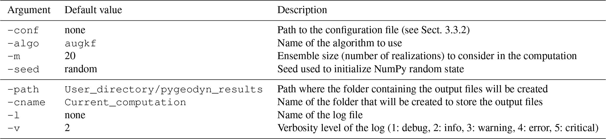
Computations can be launched by running run_algo.py that accepts several command line arguments. These arguments and their default value (taken if not supplied) are given in Table . The first group corresponds to the computation parameters, the only non-optional parameter being the path to the configuration file. The second group of parameters is linked to the output files: the name of data files and logs. We stress the importance of the argument -m that fixes the ensemble size N_e, meaning the number of realizations on which the Kalman filter will be performed. As N_e forecasts are performed at each epoch, this value has an important impact on the computation time (see Sect. 3.4). It is advised to set it to at least 20 to get a converged measure of the dispersion within the ensemble of realizations.

Table 1Command line arguments of pygeodyn/run_algo.py.

Download Print Version | Download XLSX

3.3.2 Configuration file

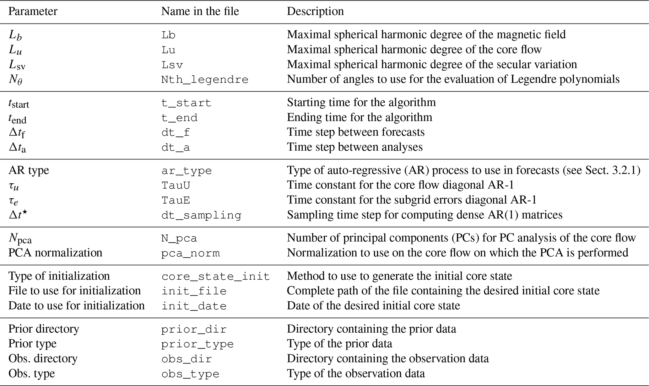
The pygeodyn configuration file sets the values of quantities used in the algorithm (called parameters). This configuration file is a text file containing three columns: one for the parameter name, one for the type and one for the parameter value. We refer to Table 2 for the list of parameters that can be set this way. The table is separated into six groups.

The first is the number of coefficients to consider for the core state quantities and the Legendre polynomials that are used to evaluate the Gaunt–Elsasser integrals that enter A(b).
The second is time spans: starting time t_start, final time t_end, and time intervals (in months) for forecasts Δt_f and analyses Δt_a. To avoid imprecise decimal representation, the times are handled with NumPy's datetime64 and timedelta64 classes (e.g., January 1980 is 1980-01¹).
The third is parameters of the AR-1 processes used in the forecasts; ar_type can be set to diag (in this case, τ_u and τ_e will be used as in Eq. 3) or to dense (in this case, Δt^⋆ will be used to sample the prior data and compute drift matrices with Eq. 5).
The fourth is parameters for using a principal component analysis (PCA) for the core flow. By setting N_pca, the algorithm will perform forecasts and analyses on the subset composed of the first N_pca principal components describing the core flow (stored by decreasing explained variance), rather than on the entire core flow model. This is advised when using dense AR-1 processes (see Gillet et al., 2019). The normalization of the PCA can be modified by setting pca_norm to energy (so that the variance of each principal component is homogeneous to a core surface kinetic energy) or to None (PCA performed directly on the Schmidt semi-normalized core flow Gauss coefficients).
The fifth is the initial conditions of the algorithm. By setting core_state_init to constant, all realizations of the initial core state will be equal to the average prior. If set to normal, realizations of the initial core state will be drawn according to a normal distribution centered on the dynamo prior average within the dynamo prior cross-covariances (default behavior). It is possible to set the initial core state to the core state from a previous computation by setting core_state_init to from_file. In this latter case, the full path of the hdf5 file of the previous computation and the date of the core state to use must be given (init_file and init_date).
The sixth is parameters describing the types of input data (priors and observations) that are presented in more detail in the next section.

Table 2Parameters available in a pygeodyn configuration file.

Download Print Version | Download XLSX

3.3.3 Priors

Priors are composed of a series of snapshot core states that are used to estimate the background states and the cross-covariance matrices. The mandatory priors are those for the magnetic field b, the core flow u and the subgrid errors e_r from which the respective cross-covariance matrices P_uu, P_ee, etc., are derived.

The aforementioned snapshots currently come from geodynamo simulations, meaning that the covariance matrices for b, u, and e_r will reflect the characteristics of the simulations. As a consequence, the forecasts will be done according to the statistics of the dynamo simulations. As examples, pygeodyn comes with two prior types derived from two simulations:

coupled_Earth from Aubert et al. (2013) and
midpath from Aubert et al. (2017).

Technically, the two types are interchangeable. However, only the midpath prior type allows for the use of dense AR-1 processes as it requires time correlations that cannot be extracted from coupled_Earth runs.

3.3.4 Observations

Observations are measurements of the magnetic field and of the SV at a set of dates. These observations are used in the analysis step to perform the BLUE of the core state (see Sect. 3.2.2). The pygeodyn package provides two types of observations:

covobs, which consists of Gauss coefficients and associated uncertainties at a series of epochs (every 6 months from 1840 to 2015) from the COV-OBS.x1 model derived by Gillet et al. (2015), and
go_vo, which consists of ground-based observatory (GO) and virtual observatory (VO) data (B_r, B_θ, B_ϕ) as well as their associated uncertainties. VOs gather in one location at satellite altitude observations recorded by the spacecraft around this site. GOs are provided every 4 months from March 1997 onward for ground-based series, and VOs every 4 months from March 2000 onward for virtual observatories. The satellite data come from the CHAMP and Swarm missions. Both VOs and GOs are cleaned as much as possible from external sources (for details, see Barrois et al., 2018; Hammer, 2018).

In the code, observation data are to be supplied with the observation operator and errors in the form of an Observation object. This allows for a consistent interface between spectral data (covobs) and data recorded in the direct space (go_vo).

3.3.5 Beyond the supplied data

For advanced users, pygeodyn provides the possibility to define custom prior and observation types by supplying new data-reading methods in the dedicated pygeodyn modules. Defining a custom prior type allows for the use of custom geodynamo simulation data to compute covariance matrices that will be used in the forecasts and analyses steps. Similarly, a new observation type can be supplied with custom observation data that will be used to estimate the core state in the analysis step.

In other words, an advanced user can completely control the input data of the algorithm to test new magnetic observations and/or new numerical models and derive new predictions from them.

3.4 Runtime scaling

To reduce computation time, supplied algorithms use MPI to perform forecasts (Sect. 3.2.1) of different realizations in parallel. Analysis steps are not implemented in parallel, as they require the whole ensemble of realizations. To assert the effect of this parallelization, model computations were performed on a varying number of cores. The configuration for this benchmark reanalysis is the following: the AugKF algorithm with diagonal AR-1 processes using m=50 realizations over $t_{end} - t_{start} = 60$ years, Δt_f=6 months and Δt_a=12 months.

The results are displayed in Fig. 1 with runtimes varying between 0.5 and 6 h. The power-law fit appears to be close to 1∕n (with n the number of cores), with an offset time of around 15 min that is probably associated with the 60 analysis steps whose duration does not depend upon the number of cores. Note that the computations remain tractable whatever the number of cores. A basic sequential computation (n=1) for a reanalysis using 50 realizations over 100 years is performed in less than 6 h, while using 32 cores will reduce it to half an hour.

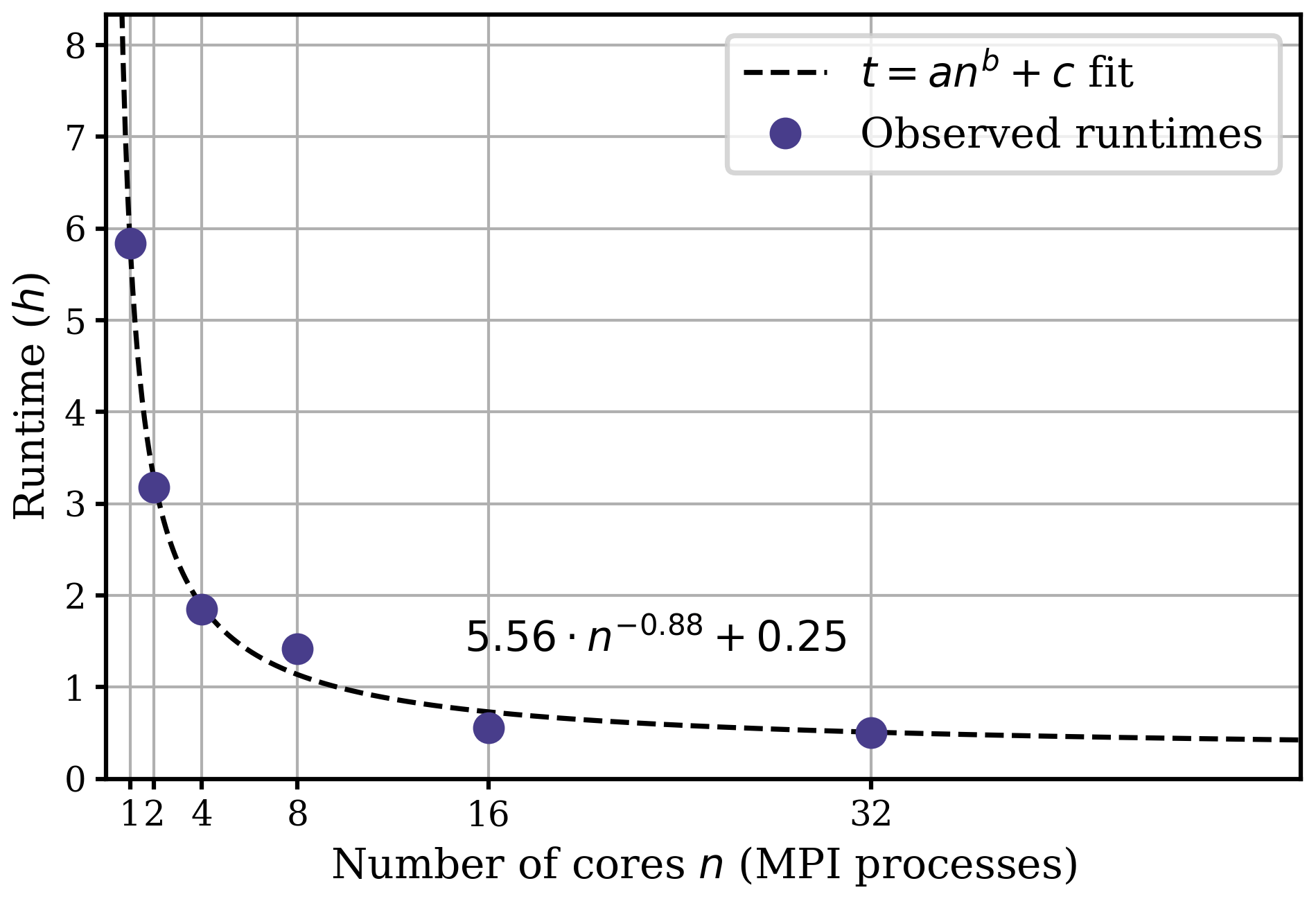
https://www.geosci-model-dev.net/12/3795/2019/gmd-12-3795-2019-f01

Figure 1Evolution of the runtime with respect to the number of MPI processes (see text for details). Dots are the observed runtimes (in hours) and the dashed line is a fit of the form $t = a \cdot n^{b} + c$ .

Download

4 Visualization

The pygeodyn output files are directly supported by the web-based visualization package webgeodyn, also developed in our group. The source code of webgeodyn is hosted at its own Git repository (https://gricad-gitlab.univ-grenoble-alpes.fr/Geodynamo/webgeodyn, last access: 12 August 2019). Being available on the Python package index, it can also be installed through the Python package installer pip.

The webgeodyn package implements a web application with several modes of representation to explore, display and diagnose the products of the reanalyses (Barrois et al., 2018). It is deployed at http://geodyn.univ-grenoble-alpes.fr (last access: 12 August 2019) but can also be used locally on any pygeodyn data, once installed. We illustrate here several possibilities offered by version 0.6.0 of this tool (Huder et al., 2019 b).

4.1 Mapping on Earth's globe projections

Quantities at a given time can be displayed at the core surface in the Earth's core surface tab. Two representations can be used simultaneously: a representation with stream dots and streamlines for the core flow components (orthoradial, azimuthal and norm) and a color plot for all quantities (core flow horizontal divergence and components included). A time slider allows the user to change the epoch at which the quantities are evaluated. Figure 2 shows an example with magnetic field as a color plot and the norm of the core flow for the streamlines for a reanalysis of VO and GO data using a diagonal AR-1 model. The plot is interactive with zooming, exporting (as pictures or animations) and display tuning features.

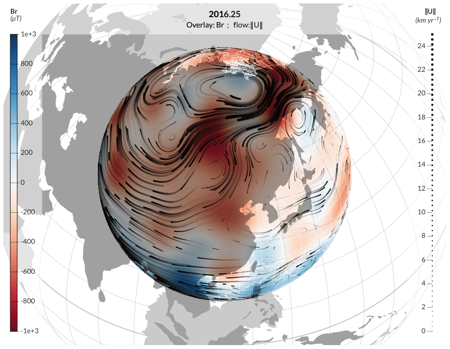
https://www.geosci-model-dev.net/12/3795/2019/gmd-12-3795-2019-f02

Figure 2Example map for the magnetic field and the flow at the core surface, obtained using webgeodyn, for the model calculated by Barrois et al. (2019). Here the radial magnetic field (color scale) and streamlines for the core flow (black lines, for which thickness indicates the intensity) are evaluated in 2016 from VO derived from the Swarm data.

4.2 Time series of harmonic coefficients

In the Spherical harmonics tab, it is possible to look at the time evolution of a single spherical harmonic coefficient for a given quantity (core flow, magnetic field, SV) or of the length of day. Several models can be displayed at once for comparison. Figure 3 shows the time evolution of one SV coefficient from a reanalysis of SV Gauss coefficient data using a dense AR-1 model. The interface gives the possibility to also represent the contribution from e_r. It is possible to zoom in on the plot and export it as a picture or raw comma-separated value (CSV) data.

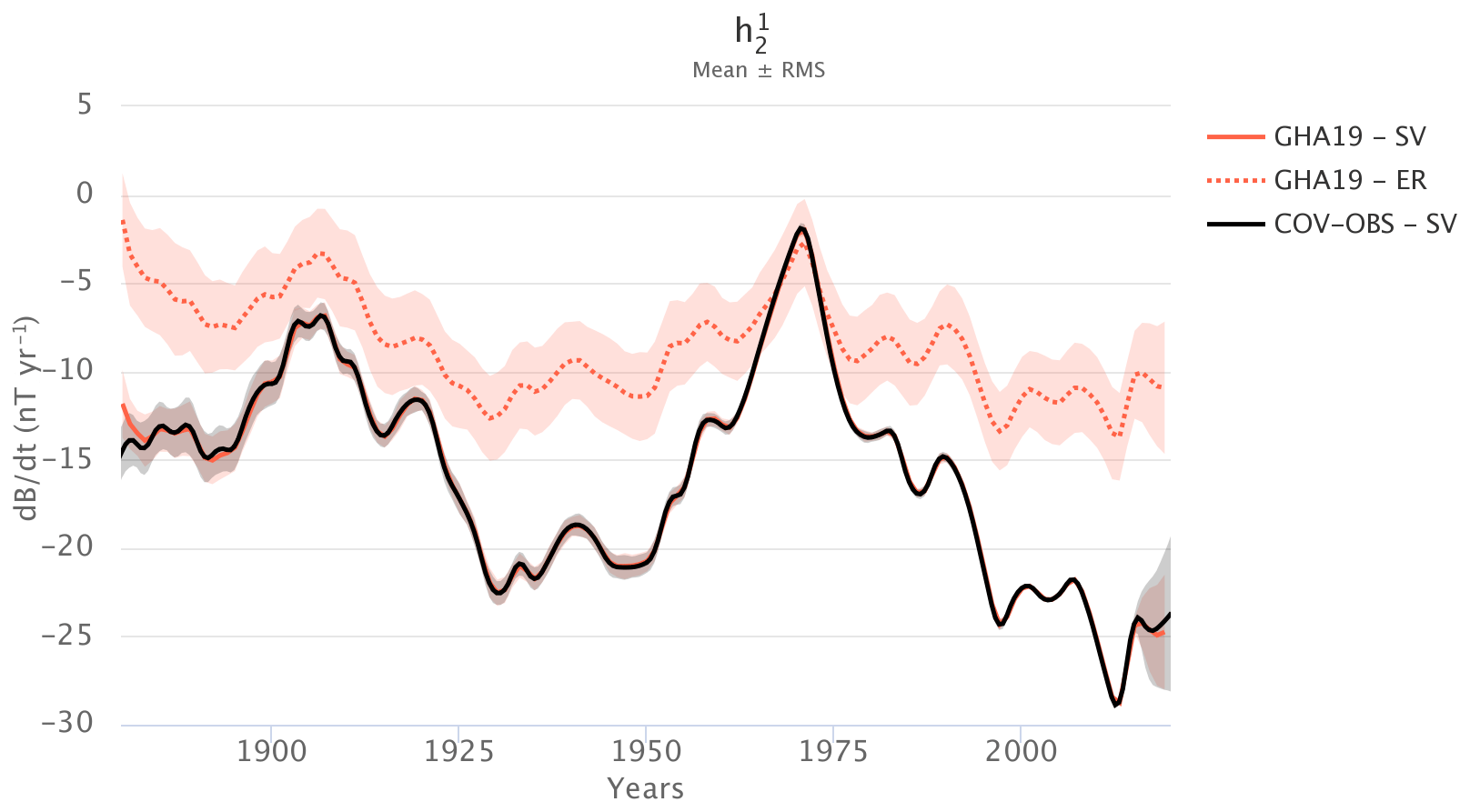
https://www.geosci-model-dev.net/12/3795/2019/gmd-12-3795-2019-f03

Figure 3Time series for the SV spherical harmonic coefficient $h_{2}^{1}$ using webgeodyn. In red (GHA19) is the reanalysis by Gillet et al. (2019), obtained from the COV-OBS.x1 observations (in black) by Gillet et al. (2015). The solid lines represent the ensemble average, and the shaded areas the ±1σ uncertainties. The dotted line gives the contribution from e_r.

Download

4.3 Comparison with ground-based and virtual observatory data

Computed data can be easily compared with the geomagnetic observations used for the analysis in the Observatory data tab. It allows the user to display the spatial components (radial, azimuthal and orthoradial) of the magnetic field and its SV recorded by observatories. These can be either GO or VO data. Data can be displayed by clicking on a location on the globe and be compared with spectral model data predictions evaluated at the observatory location. Figure 4 shows an example of the SV at a ground-based site in South America. One can compare how predictions from a reanalysis, together with its associated uncertainties, follow geophysical data (black dots) – here we show the model by Barrois et al. (2019), which uses a diagonal AR-1 model from GO and VO series. It can also be used to compare predictions from several magnetic field models – here we show COV-OBS.x1, which is constrained by magnetic data only up to 2014.5.

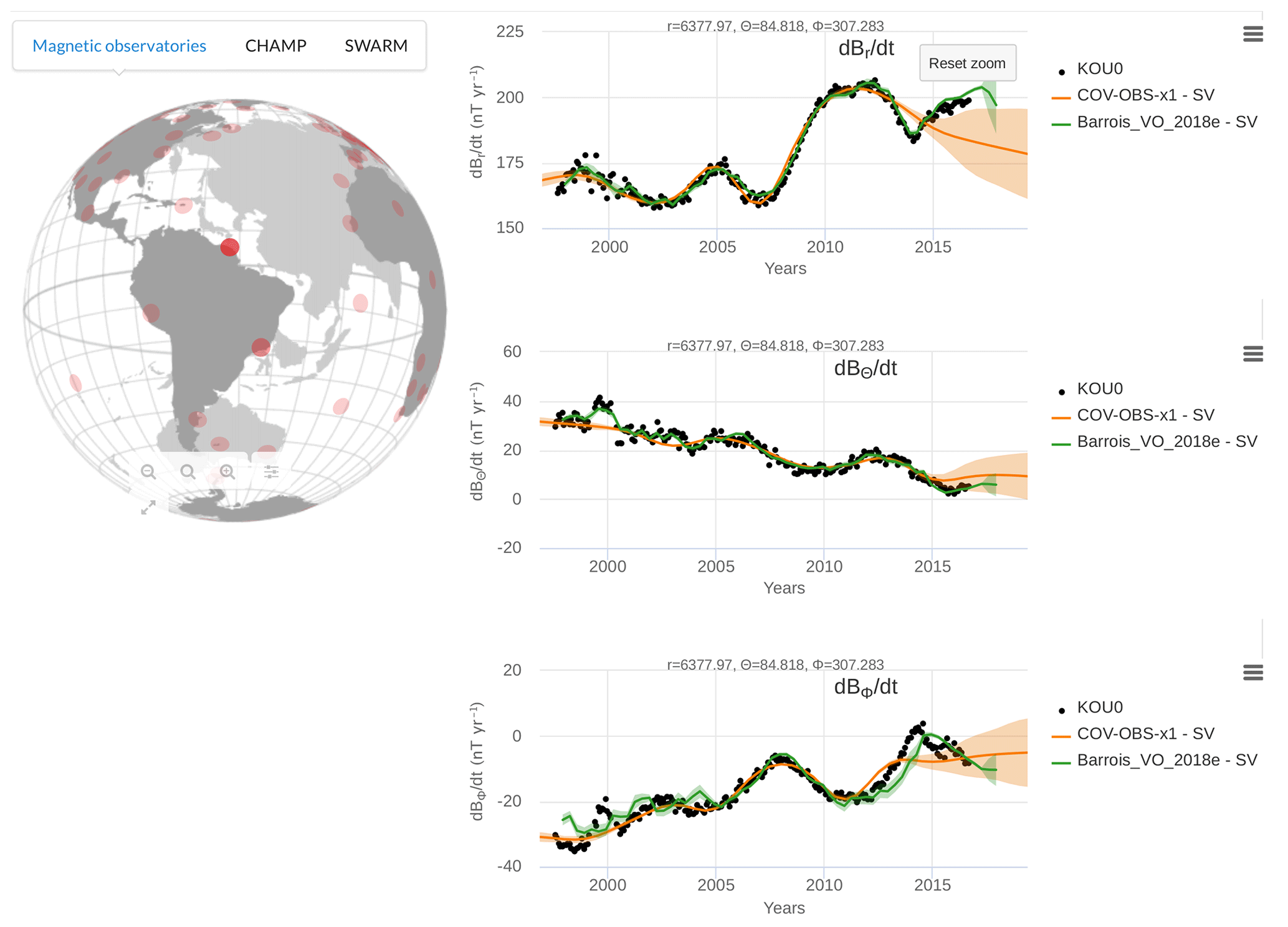
https://www.geosci-model-dev.net/12/3795/2019/gmd-12-3795-2019-f04

Figure 4Time series of the three components of the SV (in spherical coordinates) at the Kourou observatory (French Guyana, location in dark red on the globe on the left) using webgeodyn. The green line (Barrois_VO_2018e) is from the core surface reanalysis by Barrois et al. (2019), using as observations GO and VO data, and a diagonal AR-1 model. For comparison (in orange) the COV-OBS.x1 model predictions at this site are also shown. The solid lines are the ensemble mean, and the shaded areas represent the ±1σ uncertainties.

On top of the three examples illustrated above, the package webgeodyn also gives the possibility to display and export Lowes–Mauersberger spatial spectra or cross sections at the core surface as a function of time and longitude (latitude) for a given latitude (longitude).

5 Conclusions

We presented the Python toolkit pygeodyn that allows users to

calculate models of the flow at the core surface from SV Gauss coefficient data,
calculate models of the flow and the magnetic field at the core's surface from measurements of the magnetic field and its SV above the Earth's surface, and
represent and analyze the results via the web interface webgeodyn.

The underlying algorithm relies on AR-1 stochastic processes to advect the model in time. It is anchored to statistics (in space and optionally in time) from free runs of geodynamo models. It furthermore accounts for errors of representativeness due to the finite resolution of the magnetic and velocity fields.

This Python tool has been designed with several purposes in mind, among which are

tests of the Earth-likeness of geodynamo models,
comparisons with alternative geomagnetic DA algorithms,
the production of magnetic models under some constraints from the core dynamics, and
the education of students on issues linked to core dynamics and the geomagnetic inverse problem.

Code and data availability

Version 1.1.0 of pygeodyn is archived on Zenodo at https://doi.org/10.5281/zenodo.3269674 (Huder et al., 2019 a). Other versions (with or without data) are available on the Git repository located at https://gricad-gitlab.univ-grenoble-alpes.fr/Geodynamo/pygeodyn (Geodynamo, 2019 a). Version 0.6.0 of webgeodyn used for the plots is archived at https://doi.org/10.5281/zenodo.2645025 (Huder et al., 2019 b). This version (and others) can be installed from the Git repository (https://gricad-gitlab.univ-grenoble-alpes.fr/Geodynamo/webgeodyn, Geodynamo, 2019 b) or as a Python package with pip. Data sets can be downloaded at http://geodyn.univ-grenoble-alpes.fr (Geodynamo, 2019 c) or on the Git repository at https://gricad-gitlab.univ-grenoble-alpes.fr/Geodynamo/pygeodyn_data (Geodynamo, 2019 d).

Author contributions

The scientific development of the presented package was done by NG and LH. The technical development (including tests and packaging) was done by LH and FT. All authors contributed to the writing of the paper.

Competing interests

The authors declare that they have no conflict of interest.

Acknowledgements

We thank Julien Aubert for supplying the geodynamo series used as priors and Christopher Finlay and Magnus Hammer for providing the go_vo data. We are grateful to Nathanaël Schaeffer for helpful comments on the paper. We thank the national institutes that support ground magnetic observatories and INTERMAGNET for promoting high standards of practice and making the data available.

Financial support

This work is partially supported by the French Centre National d'Etudes Spatiales (CNES) in the context of the Swarm mission of the ESA.

Review statement

This paper was edited by Josef Koller and reviewed by Ciaran Beggan and one anonymous referee.

References

Aubert, J., Finlay, C. C., and Fournier, A.: Bottom-up Control of Geomagnetic Secular Variation by the Earth's Inner Core, Nature, 502, 219–223, https://doi.org/10.1038/nature12574, 2013. a, b

Aubert, J., Gastine, T., and Fournier, A.: Spherical Convective Dynamos in the Rapidly Rotating Asymptotic Regime, J. Fluid Mech., 813, 558–593, https://doi.org/10.1017/jfm.2016.789, 2017. a, b, c

Bärenzung, J., Holschneider, M., Wicht, J., Sanchez, S., and Lesur, V.: Modeling and Predicting the Short-Term Evolution of the Geomagnetic Field, J. Geophys. Res.-Sol. Ea., 123, 4539–4560, https://doi.org/10.1029/2017JB015115, 2018. a

Barrois, O., Gillet, N., and Aubert, J.: Contributions to the Geomagnetic Secular Variation from a Reanalysis of Core Surface Dynamics, Geophys. J. Int., 211, 50–68, https://doi.org/10.1093/gji/ggx280, 2017. a, b, c, d

Barrois, O., Hammer, M. D., Finlay, C. C., Martin, Y., and Gillet, N.: Assimilation of Ground and Satellite Magnetic Measurements: Inference of Core Surface Magnetic and Velocity Field Changes, Geophys. J. Int., 215, 695–712, https://doi.org/10.1093/gji/ggy297, 2018. a, b, c, d

Barrois, O., Gillet, N., Aubert, J., Barrois, O., Hammer, M. D., Finlay, C. C., Martin, Y., and Gillet, N.: Erratum: “Contributions to the Geomagnetic Secular Variation from a Reanalysis of Core Surface Dynamics” and “Assimilation of Ground and Satellite Magnetic Measurements: Inference of Core Surface Magnetic and Velocity Field Changes”, Geophys. J. Int., 216, 2106–2113, https://doi.org/10.1093/gji/ggy471, 2019. a, b, c, d, e

Evensen, G.: The Ensemble Kalman Filter: Theoretical Formulation and Practical Implementation, Ocean Dynam., 53, 343–367, https://doi.org/10.1007/s10236-003-0036-9, 2003. a

Evensen, G.: Data Assimilation: The Ensemble Kalman Filter, Springer Science & Business Media, 2009. a

Finlay, C. C., Olsen, N., Kotsiaros, S., Gillet, N., and Tøffner-Clausen, L.: Recent Geomagnetic Secular Variation from Swarm and Ground Observatories as Estimated in the CHAOS-6 Geomagnetic Field Model, Earth Planet. Space, 68, 112, https://doi.org/10.1186/s40623-016-0486-1, 2016. a

Finlay, C. C., Lesur, V., Thébault, E., Vervelidou, F., Morschhauser, A., and Shore, R.: Challenges Handling Magnetospheric and Ionospheric Signals in Internal Geomagnetic Field Modelling, Space Sci. Rev., 206, 157–189, https://doi.org/10.1007/s11214-016-0285-9, 2017. a

Fournier, A., Hulot, G., Jault, D., Kuang, W., Tangborn, A., Gillet, N., Canet, E., Aubert, J., and Lhuillier, F.: An Introduction to Data Assimilation and Predictability in Geomagnetism, Space Sci. Rev., 155, 247–291, https://doi.org/10.1007/s11214-010-9669-4, 2010. a

Geodynamo: Geodynamo / pygeodyn, available at: https://gricad-gitlab.univ-grenoble-alpes.fr/Geodynamo/pygeodyn, last access: 12 August 2019a. a

Geodynamo: Geodynamo / webgeodyn, available at: https://gricad-gitlab.univ-grenoble-alpes.fr/Geodynamo/webgeodyn, last access: 12 August 2019b. a

Geodynamo: Geodyn, available at: http://geodyn.univ-grenoble-alpes.fr last access: 12 August 2019c. a

Geodynamo: Geodynamo / pygeodyn_data, available at: https://gricad-gitlab.univ-grenoble-alpes.fr/Geodynamo/pygeodyn_data last access: 12 August 2019d. a

Gillet, N.: Spatial And Temporal Changes Of The Geomagnetic Field: Insights From Forward And Inverse Core Field Models, in: Geomagnetism, Aeronomy and Space Weather: A Journey from the Earth's Core to the Sun, edited by: Mandea, M., Korte, M., Petrovsky, E., and Yau, A., arXiv:1902.08098[physics], 2019. a

Gillet, N., Barrois, O., and Finlay, C. C.: Stochastic Forecasting of the Geomagnetic Field from the COV-OBS.X1 Geomagnetic Field Model, and Candidate Models for IGRF-12, Earth Planet. Space, 67, 71, https://doi.org/10.1186/s40623-015-0225-z, 2015. a, b

Gillet, N., Huder, L., and Aubert, J.: A Reduced Stochastic Model of Core Surface Dynamics Based on Geodynamo Simulations, Geophys. J. Int., 1, 522–539, https://doi.org/10.1093/gji/ggz313, 2019. a, b, c, d, e

Hammer, M. D.: Local Estimation of the Earth's Core Magnetic Field, PhD thesis, Technical University of Denmark (DTU), 2018. a

Huder, L., Gillet, N., and Thollard, F.: Pygeodyn 1.1.0: A Python Package for Geomagnetic Data Assimilation, https://doi.org/10.5281/zenodo.3269674, 2019a. a, b

Huder, L., Martin, Y., Thollard, F., and Gillet, N.: Webgeodyn 0.6.0: Visualisation Tools for Motions at the Earth's Core Surface, https://doi.org/10.5281/zenodo.2645025, 2019b. a, b

Kalnay, E.: Atmospheric Modeling, Data Assimilation and Predictability, Cambridge university press, 2003. a

Moon, W.: Numerical Evaluation of Geomagnetic Dynamo Integrals (Elsasser and Adams-Gaunt Integrals), Comput. Phys. Commun., 16, 267–271, https://doi.org/10.1016/0010-4655(79)90092-4, 1979. a

Sanchez, S., Wicht, J., Bärenzung, J., and Holschneider, M.: Sequential Assimilation of Geomagnetic Observations: Perspectives for the Reconstruction and Prediction of Core Dynamics, Geophys. J. Int., 217, 1434–1450, 2019. a

Schaeffer, N., Jault, D., Nataf, H.-C., and Fournier, A.: Turbulent Geodynamo Simulations: A Leap towards Earth's Core, Geophys. J. Int., 211, 1–29, https://doi.org/10.1093/gji/ggx265, 2017. a, b

More precisely, 1 January 1980.

Articles

Short summary

The pygeodyn package is a geomagnetic data assimilation tool written in Python. It gives access to the Earth's core flow dynamics, controlled by geomagnetic observations, by means of a reduced numerical model anchored to geodynamo simulation statistics. It aims to provide the community with a user-friendly and tunable data assimilation algorithm. It can be used for education, geomagnetic model production or tests in conjunction with webgeodyn, a set of visualization tools for geomagnetic models.