the Creative Commons Attribution 4.0 License.
the Creative Commons Attribution 4.0 License.
 | 02 Sep 2019
Improved methodologies for Earth system modelling of atmospheric soluble iron and observation comparisons using the Mechanism of Intermediate complexity for Modelling Iron (MIMI v1.0)
Rachel A. Scanza
Joseph Guinness
Jasper F. Kok
Longlei Li
Xiaohong Liu
Sagar D. Rathod
Jessica S. Wan
Mingxuan Wu
Natalie M. Mahowald
Herein, we present a description of the Mechanism of Intermediate complexity for Modelling Iron (MIMI v1.0). This iron processing module was developed for use within Earth system models and has been updated within a modal aerosol framework from the original implementation in a bulk aerosol model. MIMI simulates the emission and atmospheric processing of two main sources of iron in aerosol prior to deposition: mineral dust and combustion processes. Atmospheric dissolution of insoluble to soluble iron is parameterized by an acidic interstitial aerosol reaction and a separate in-cloud aerosol reaction scheme based on observations of enhanced aerosol iron solubility in the presence of oxalate. Updates include a more comprehensive treatment of combustion iron emissions, improvements to the iron dissolution scheme, and an improved physical dust mobilization scheme. An extensive dataset consisting predominantly of cruise-based observations was compiled to compare to the model. The annual mean modelled concentration of surface-level total iron compared well with observations but less so in the soluble fraction (iron solubility) for which observations are much more variable in space and time. Comparing model and observational data is sensitive to the definition of the average as well as the temporal and spatial range over which it is calculated. Through statistical analysis and examples, we show that a median or log-normal distribution is preferred when comparing with soluble iron observations. The iron solubility calculated at each model time step versus that calculated based on a ratio of the monthly mean values, which is routinely presented in aerosol studies and used in ocean biogeochemistry models, is on average globally one-third (34 %) higher. We redefined ocean deposition regions based on dominant iron emission sources and found that the daily variability in soluble iron simulated by MIMI was larger than that of previous model simulations. MIMI simulated a general increase in soluble iron deposition to Southern Hemisphere oceans by a factor of 2 to 4 compared with the previous version, which has implications for our understanding of the ocean biogeochemistry of these predominantly iron-limited ocean regions.
- Article
(23524 KB) -
Supplement
(818 KB) - BibTeX
- EndNote


Iron is an essential micronutrient for ocean primary productivity (Martin et al., 1991; Martin, 1990). Iron deficiency in oceans leads to high-nutrient low-chlorophyll (HNLC) conditions under which the photosynthetic productivity of phytoplankton is iron limited (Boyd et al., 2007; Jickells et al., 2005), and in other regions iron may be an important nutrient for nitrogen fixation by diazotrophs (Capone et al., 1997; Moore et al., 2013, 2006). Atmospheric deposition of bioavailable iron (i.e. the fraction of the total iron deposited that is readily available for ocean biota uptake) contained in aerosol is an important source of new iron for the remote open ocean (Duce and Tindale, 1991; Fung et al., 2000); therefore, iron impacts the ability of oceans to act as a sink of atmospheric carbon dioxide (Jickells et al., 2014; Moore et al., 2013).
Several definitions for bioavailable iron have been proposed. The solubility of iron is considered to be a key factor modulating its bioavailability (Baker et al., 2006a, b); therefore, we consider bioavailable iron to be dissolved (labile) iron in either a (II) or (III) oxidation state, and we define this as the soluble iron concentration throughout the paper. However, since most aerosol iron is insoluble at emission the processing of insoluble iron to a soluble form must occur during atmospheric transport. The acidic processing of iron contained in aerosol is one pathway through which soluble iron can be liberated from an insoluble form with decreasing pH (Duce and Tindale, 1991; Solmon et al., 2009; Zhu et al., 1997). Organic ligands, in particular oxalate, also increase iron solubility by weakening or cleaving the Fe–O bonds found in iron oxide minerals via complexation (Li et al., 2018; Panias et al., 1996), and in nature this reaction proceeds most rapidly in a slightly acidic aqueous medium, such as cloud droplets (Cornell and Schindler, 1987; Paris et al., 2011; Xu and Gao, 2008). Organic ligand processing has been estimated to increase soluble iron concentrations by up to 75 % more than is achievable with acid processing alone (Ito, 2015; Johnson and Meskhidze, 2013; Myriokefalitakis et al., 2015; Scanza et al., 2018). However, there is no single mechanism that describes the observed inverse relationship of higher iron solubilities with decreasing iron concentrations (Sholkovitz et al., 2012). Rather, Mahowald et al. (2018) used a 1-D plume model to demonstrate that the observed trend can be explained by either the differences in iron solubility at emission or the atmospheric dissolution of insoluble iron. Thus, there is no observational constraint to indicate which is more likely unless spatial distribution is also considered.
The recent increase in efforts to model iron solubility (Ito, 2015; Ito and Xu, 2014; Johnson and Meskhidze, 2013; Luo et al., 2008; Meskhidze et al., 2005; Myriokefalitakis et al., 2015; Scanza et al., 2018) reflects its importance for understanding biogeochemical cycles (Andreae and Crutzen, 1997; Arimoto, 2001; Jickells et al., 2005; Mahowald, 2011) and how human activity may be perturbing them (Mahowald et al., 2009, 2017). However, the multifaceted nature of how iron interacts within the Earth system results in many uncertainties regarding how to best represent the atmospheric iron cycle within models, which are themselves of varying complexity (Myriokefalitakis et al., 2018). To incorporate the processes currently thought to be the most significant (Journet et al., 2008; Meskhidze et al., 2005; Paris et al., 2011; Shi et al., 2012) and improve model-to-observation comparisons of the soluble iron fraction, particularly in remote ocean regions (Baker et al., 2006b; Ito, 2015; Mahowald et al., 2018; Matsui et al., 2018; Sholkovitz et al., 2012), model development has been focused on refining the atmospheric iron emission sources and subsequent atmospheric processing (Ito, 2015; Ito and Xu, 2014; Johnson and Meskhidze, 2013; Luo et al., 2008; Meskhidze et al., 2005; Myriokefalitakis et al., 2015; Scanza et al., 2018).
A recent multi-model evaluation of four global atmospheric iron cycle models (Myriokefalitakis et al., 2018) showed that total iron deposition is overrepresented close to major dust source regions and underrepresented in remote regions compared with observations from all four models. This is consistent with previous model intercomparison studies that demonstrated the difficulty of simultaneously simulating both atmospheric concentrations and deposition fluxes of desert dust (Huneeus et al., 2011). Importantly, none of the atmospheric iron processing models can capture the high (>10 %) solubilities measured over the Southern Ocean; this is potentially because the model processes associated with transport and ageing of aerosol iron require further development (Ito et al., 2019). Conclusions from Myriokefalitakis et al. suggest that future model improvements should focus on a more realistic aerosol size distribution and the representation of mineral-to-combustion sources of iron. Most of the development of the Mechanism of Intermediate complexity for Modelling Iron (MIMI), as described herein, focused on these points. First, we transitioned from a bulk aerosol scheme to a two-moment modal aerosol scheme (Liu et al., 2012), and second, we re-evaluated pyrogenic iron emissions from anthropogenic combustion and fires. The modal aerosol scheme was used to calculate both aerosol mass and number at each time step within an updated global aerosol microphysics model, and both the fire and anthropogenic combustion emissions from Luo et al. (2008), which are likely to be underestimated (Conway et al., 2019; Ito et al., 2019; Matsui et al., 2018), were improved upon.
Ocean observations of iron and its soluble fraction are limited both spatially and temporally owing to the significant costs and logistical constraints associated with accumulating data from scientific cruises. Thus, there is an inherent disparity in attempting to compare climatological means calculated from temporally chronological model results with observational means calculated from temporally limited and sporadic observations (e.g. Mahowald et al., 2008, 2009). This is important because natural aerosol emissions are variable on seasonal, annual, and decadal timescales in terms of both primary natural iron emission sources (mineral dust and wildfires) and the source of aerosol acidity. For example, sulfuric acid from the oxidation of dimethyl sulfide and fire SO2 (Bates et al., 1992; Chin and Jacob, 1996) has been observed to aid iron dissolution when far from anthropogenic acid sources (Zhuang et al., 1992). The limitations associated with the collection of continuous annual or inter-annual ship-based data across multiple remote ocean regions are immutable at present, which hinders the required derivation of the basic statistical properties of such highly variable data (Smith et al., 2017). Attention could therefore be given to the methodologies with which such model–observation comparisons are undertaken instead.
The paper is presented in four parts. The first part (Sect. 2) introduces updates made to the Bulk Aerosol Module (BAM) iron scheme of Scanza et al. (2018) and its implementation within the Modal Aerosol Module (MAM), with four modes (MAM4), within the Community Earth System Model (CESM). In the second part (Sect. 3), we compare iron concentrations and the fractional solubility of iron with the observational data. Then the third part (Sect. 4) compares our updated version of the model with its predecessor. Finally, we suggest further developments for atmospheric iron modelling and for comparing model results with sporadic observations (Sect. 5).
The present study improves upon the previous atmospheric iron cycle module developed for the Community Atmosphere Model (CAM) version 4 (CAM4) embedded in the CESM; we will refer to this version as BAM-Fe (Scanza et al., 2015, 2018) herein. We incorporated the iron module within the MAM framework (Liu et al., 2012, 2016) currently in the Department of Energy's Energy Exascale Earth System Model (E3SM; Golaz et al., 2019) and the CAM versions 5 and 6 (CESM-CAM5–6; Neale et al., 2010); we refer to this new version of the iron model by its name (MIMI) herein. Table 1 serves as a reference and summarizes the modifications made for MIMI, which are discussed throughout the paper.
Table 1Short summary of major differences between BAM-Fe and MIMI.
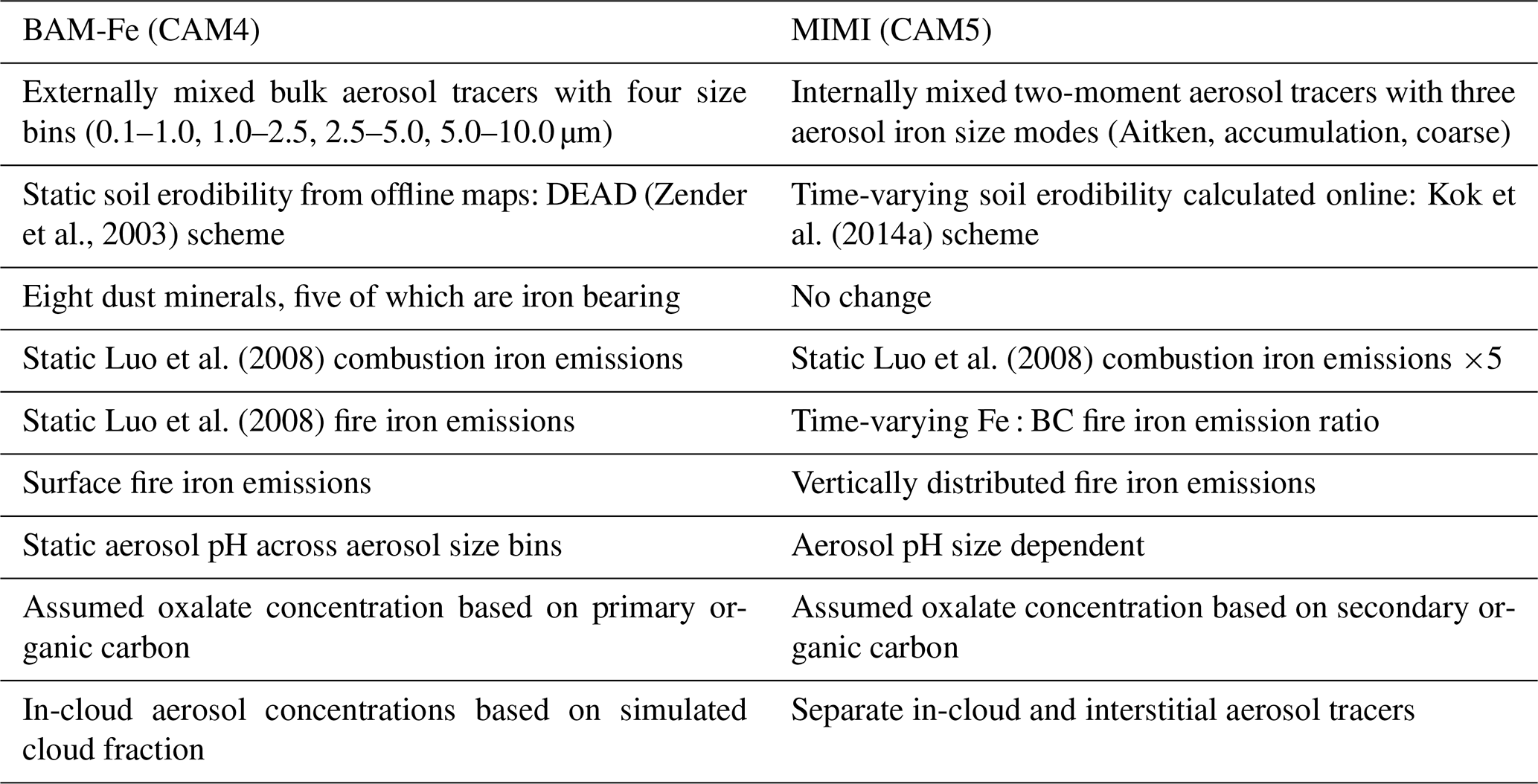
Table 2Combustion iron aerosol size and number properties.
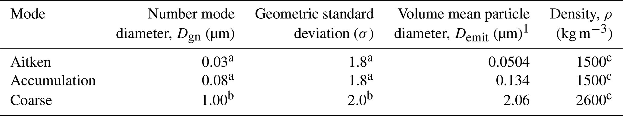
1 . a Liu et al. (2012). b Dentener et al. (2006) and Liu et al. (2012). c Wang et al. (2015).
We use MAM4 with four simulated log-normal aerosol size modes: three modes (Aitken, accumulation, and coarse) containing iron and a fourth primary carbonaceous mode. Table 2 details the new pyrogenic iron (i.e. from fires and anthropogenic combustion) modal aerosol properties, while those of mineral dust iron follow existing dust aerosol properties (Liu et al., 2012). Generally, the modelled density of iron is similar to size-resolved ambient aerosol densities measured in eastern China (Hu et al., 2012), which has significant dust and combustion aerosol sources. MIMI was initially implemented and tested within a development branch of CAM 5.3, as per Wu et al. (2017, 2018), using Cheyenne (Computational and Information Systems Laboratory, 2017) and closely resembles CESM version 1.2.2. We used a horizonal (longitude by latitude) resolution and 56 vertical layers up to 2 hPa. Stratiform microphysics followed a two-moment cloud microphysics scheme (Gettelman et al., 2010; Morrison and Gettelman, 2008). The other major aerosol species black carbon (BC), organic carbon, sea salt, and sulfate (SO4) were also simulated but are not explicitly examined here because we are focused on iron aerosol modelling. However, atmospheric iron processing in MIMI requires both sulfate and (secondary) organic aerosols to be simulated as they act as proxies for the reactant species of [H+] and oxalate, respectively. In CAM5 sulfate aerosol is present in all three hydrophilic aerosol modes, while secondary organic aerosol is only present in the fine Aitken and accumulation modes (Liu et al., 2012, 2016). Aerosol microphysics was applied in the same way to the new iron aerosol tracers as the base aerosol species (Liu et al., 2012, 2016). Fire emissions were vertically distributed between six injection height ranges: 0–0.1, 0.1–0.5, 0.5–1.0, 1.0–2.0, 2.0–3.0, and 3.0–6.0 km, as per AeroCom recommendations (Dentener et al., 2006). Fire emissions were uniformly distributed in model levels between height limits. Unless otherwise stated, aerosol and precursor gas mass emissions were from the Climate Model Intercomparison Program (CMIP5) inventory (Lamarque et al., 2010). Major gas-phase oxidants (O3, OH, NO3, and HO2) were supplied offline and were also from Lamarque et al. (2010). Meteorology (U, V, and T) was nudged to Modern-Era Retrospective analysis for Research and Applications (MERRA) data for 2006–2011. Unless otherwise stated, the last 5 years were used for analysis.
The model used in this study performed well when compared to observations from a variety of different environments and produced aerosol concentrations that were close to those of the multi-model mean of similarly complex aerosol models (Fanourgakis et al., 2019).
2.1 Dust aerosol modelling
Mineral dust aerosol was modelled via the Dust Entrainment and Deposition model (DEAD; Zender et al., 2003), which was previously updated to include the brittle fragmentation theory of vertical dust flux (Kok, 2011) on mineral size fractions (Albani et al., 2014; Scanza et al., 2015). We further improved the emissions of dust in MAM to follow a physically based vertical flux theory (Kok et al., 2014a), which has been shown to significantly improve dust emissions (Kok et al., 2014b). Note that this method allowed for the removal of the soil erodibility map approach previously employed by the DEAD scheme (Table 1) and still provided more accurate simulations of regional dust emissions and concentrations (Kok et al., 2014b). Dust aerosol optical depth (AOD) was calculated using mineralogy-based radiation interactions as described by Scanza et al. (2015). Dust emissions were tuned such that a global annual mean dust AOD of ∼0.03 was attained, as recommended by Ridley et al. (2016) and matching values in Scanza et al. (2015) for a similar model configuration.
Dust mineralogy in MIMI is designed to be comprised of eight separate transported tracers: illite, kaolinite, montmorillonite, hematite, quartz, calcite, feldspar, and gypsum (Scanza et al., 2015). Mineral soil distributions were supplied offline (Claquin et al., 1999) with the emission of each dust mineral species further refined following the brittle fragmentation theory (Scanza et al., 2015).
2.2 Iron aerosol modelling
The simulated life cycle of iron can be grouped into three main stages: (1) iron emission to the atmosphere, (2) physical–chemical iron processing during transport, and (3) final iron deposition and thus loss from the atmosphere. In the following sections, we describe the emissions and subsequent atmospheric dissolution of iron (stages 1 and 2), while the effects of this on the magnitude of oceanic soluble iron deposition (stage 3) in MIMI are examined and compared to BAM-Fe in Sect. 4.
Iron optical properties are currently considered to reflect those of hematite because this mineral contains 97 % of the iron aerosol mass fraction (see Sect. 2.3.1).
2.3 Iron aerosol emissions
MIMI contains three major iron emission sources: mineral dust, fires (defined here as the sum of wildfires and human-mediated biomass burning), and anthropogenic combustion (defined here as the sum of industrial and domestic biofuel burning). In the BAM-Fe version of the model, fire and anthropogenic combustion emissions were combined into a single static monthly mean value. In MIMI, fire emissions of iron were updated to be distinct from other pyrogenic iron sources and were parameterized to track the BC emissions from fires using an Fe : BC ratio. Fire BC emissions were simulated to be time varying on a monthly scale, resulting in a much more pronounced seasonality to fire iron emissions (e.g. Giglio et al., 2013) compared to BAM-Fe wherein seasonality was not imposed.
For all iron species in each mode, the aerosol number emissions (Feemit,num) were calculated from the mass emissions within the same mode (Feemit,mass) using the properties in Table 2 and following Liu et al. (2012):
2.3.1 Iron emissions within mineral dust aerosol
Based on previous research by Journet et al. (2008) and Ito and Xu (2014), the iron fraction in each mineral species was prescribed at emission as follows: 57.5 % in hematite, 11 % in smectite, 4 % in illite, 0.24 % in kaolinite, 0.34 % in feldspar, and 0 % in the remaining three mineral species (Table 3), which has been shown to improve the accuracy of the modelled total iron fraction estimated from mineral dust (Scanza et al., 2018; Zhang et al., 2015). The mass of each of the eight mineral dust species advected at each model time step was the residual mineral mass (i.e. after the removal of the iron mass) such that the sum of all eight minerals and the total iron from mineral dust equalled unity and hence the original total singular dust mass emitted from the land surface.
Table 3Mass fraction of iron in each simulated iron-bearing dust mineral species and allocation to each mineral iron tracer at emission. At emission medium-soluble iron is equivalent to the fast-soluble iron fraction (i.e. the fraction which is already assumed to be soluble at emission). Residual mineral dust mass is then advected as its respective tracer.

Iron emissions from the five iron-bearing mineral dust species (three dust minerals contain no iron) were then partitioned into the four advected mineral-dust-bearing iron aerosol tracers (Table 3); iron tracers were defined as being (in)soluble and by the speed of the atmospheric reaction rate acting on them: slow or medium (Scanza et al., 2018). Note that slow- and medium-soluble iron is only produced by non-reversible atmospheric processing within the model; therefore, computational costs can be reduced by not creating a separate iron tracer representing the fraction which is already soluble at emission (i.e. “fast” reacting) but instead adding an initial medium-soluble iron processed emission burden which is equivalent to the assumed fast-reacting iron fraction.
2.3.2 Iron aerosol emissions from fires
Following Luo et al. (2008), we used observed Fe : BC mass ratios to estimate fine- and coarse-mode iron emissions from fires. An additional difference between BAM (CAM4) and MAM (CAM5) is the emission dataset used to estimate global fire emissions of aerosol and trace gases. The BAM model uses adjusted AeroCom fire emissions (Dentener et al., 2006; Scanza et al., 2018), while MAM uses CMIP5 fire emissions (Lamarque et al., 2010). Base fire BC emissions within the CMIP5 database are 2.55 Tg a−1 BC; however, the scaling of emissions from fires has been shown to be necessary to improve model-to-observed (aerosol optical depth and particulate matter) BC ratios (Reddington et al., 2016; Ward et al., 2012). Therefore, we globally scaled the fire iron emissions by a uniform factor of 2, which is comparable with the overall lower scaling factor from a review of the literature by Reddington et al. (2016; Table 2). Fine-mode iron emissions from fires were then segregated to assign 10 % of the fine-sized mass to the Aitken mode, with the remaining 90 % assigned to the accumulation mode.
Luo et al. (2008) used a single Amazonian observational dataset in their study to determine the flux of iron aerosol from fires (Fe : BC). We extended this to incorporate other Amazonian fire (Fe : BC) data and, importantly, non-Amazonian biome fire (Fe : BC) data, which are likely to have different combustion properties and hence iron emissions (e.g. Akagi et al., 2011). From Table 4, we suggest that after adding 11 more data inventory values, Luo et al. likely underrepresented the global fine-mode Fe : BC ratio at 0.02. We instead used the global mean Fe : BC ratio from the additional data of 0.06. Conversely, Luo et al. likely overrepresented the coarse-mode Fe : BC ratio at 1.4. By including additional observational information from Artaxo et al. (2013) we reduced this to 1.0. Using size-segregated wet season (i.e. representing a locally transported emission source) observation data from Artaxo et al. (2013), we estimated that the amount of BC mass in the coarse mode was 37 % of fine-mode mass. Overall this doubles the fractional contribution of fine-mode (BAM: 0.1–1 µm size bin, MAM: sum of Aitken and accumulation modes) iron emissions from fires (BAM-Fe: fine is 7 % of total mass, MIMI: fine is 14 % of total mass).
Table 4Measured iron (Fe) and black carbon (BC) values (various units; as only the Fe : BC ratio is required they are not included) and the Fe : BC ratio; calculated with three decimal places, ratio reported to one significant figure to reflect high uncertainty. Modelled fire emission ratio for Fe : BC then calculated from observed ratios.

Using the soluble Fe : BC ratio of 0.02 reported in Luo et al. (2008) resulted in 33 % solubility of fine-mode iron from fires at emission, which is lower than the 46 % reported in Oakes et al. (2012) and higher than the 12 % reported in Ito (2013). As few data exist in the literature pertaining to coarse-mode BC, or more importantly its ratio to iron, we retained the 4 % solubility of iron in the coarse mode at emission, as suggested by Luo et al.
Total iron emissions from fires in MIMI were 2.2 Tg Fe a−1 (Aitken: 0.02 Tg a−1, accumulation: 0.28 Tg a−1, coarse: 1.9 Tg a−1), representing an approximate increase in iron emissions from fires of around 25 % compared with those from BAM-Fe, with most of the mass (86 %) still in the coarse mode. The lower 25 % increase between BAM-Fe and MIMI iron emissions, compared to the doubling of the fire iron emissions themselves within MIMI, is due to different underlying fire emission inventories used in each model. Aerosol number concentrations were then calculated using Eq. (1) and the physical properties listed in Table 2. We adopted the methodology of Wang et al. (2015) by assuming that the density of iron aerosol from fires (and anthropogenic combustion) in the Aitken and accumulation modes matches that of BC, while in the coarse mode it matches that of mineral dust. The vertical distribution of iron emissions from fires was also updated in MIMI (BAM-Fe emitted all iron from fires at the surface) to account for pyro-convection, which lofts aerosol to higher altitudes at the point of emission within the model (Rémy et al., 2017; Sofiev et al., 2012; Wagner et al., 2018).
2.3.3 Iron emissions from anthropogenic combustion sources
Separate lines of evidence (Conway et al., 2019; Ito et al., 2019; Matsui et al., 2018) have shown that anthropogenic industrial iron emissions are highly likely to be larger than previously estimated (e.g. Ito, 2015; Luo et al., 2008; Myriokefalitakis et al., 2018). Therefore, anthropogenic combustion emissions of iron in MIMI were the same as those in BAM-Fe, as first reported by Luo et al. (2008), uniformly multiplied by a factor of 5 to bring them into closer agreement with observations of industrial magnetite emissions in line with Matsui et al. (2018). Resulting fine-mode anthropogenic combustion emissions were 0.50 Tg Fe a−1 and coarse-mode emissions were 2.8 Tg Fe a−1. Similar to fire emissions, 10 % of fine-sized emissions were partitioned into the Aitken mode at emission; the remaining 90 % of fine-sized emissions were emitted into the accumulation mode, and 100 % of coarse-sized emissions were emitted to the coarse mode. We retain the Luo et al. (2008) estimate of 4 % combustion iron solubility at emission (Chuang et al., 2005). Calculations of aerosol number concentrations of combustion iron followed the same procedure as described for fire emissions in Sect. 2.3.2.
2.4 Atmospheric iron aerosol processing
2.4.1 Acid and organic ligand processing
Once airborne, iron undergoes a series of physical and chemical processing steps within the atmosphere, each working to alter the soluble iron fraction (i.e. its solubility). The MIMI atmospheric iron dissolution scheme is presented in Table 5, with a full description reported previously by Scanza et al. (2018). Within each of the three iron-bearing aerosol size modes, six tracers of iron were advected within the model: medium-insoluble and medium-soluble mineral dust iron (containing both readily released and medium-reactive mineral dust iron; Scanza et al., 2018), slow-insoluble and slow-soluble mineral dust iron, and insoluble and soluble pyrogenic (sum of fires and anthropogenic combustion) iron, which was assumed to be medium-reactive (Scanza et al., 2018). Both proton- and organic-ligand-promoted iron dissolution mechanisms were modelled. The proton-promoted dissolution scheme was dependent upon an estimated [H+], calculated from the ratio of sulfate to calcite, and the simulated temperature. Organic ligand dissolution was dependent upon the simulated secondary organic carbon concentration as oxalate (the main reactant) itself was not modelled. Both the sulfate and secondary organic carbon aerosol (Fig. S1 in the Supplement), which the iron processing requires, are fundamental components of aerosol models (e.g. Kanakidou et al., 2005; Mann et al., 2014). In CAM sulfate is mainly formed via the oxidation of SO2(aq) with a smaller contribution from H2SO4 condensation on aerosol, while secondary organic aerosol is formed via the partitioning of semi-volatile organic gases (Liu et al., 2012). Neither gas-to-particle production processes are structurally modified from the description of CAM5 by Liu et al. (2012, 2016) by the incorporation of MIMI. A structural model improvement was that MAM (CAM5) advected separate tracers for the interstitial and cloud-borne aerosol phases, so the proton- and organic-ligand-promoted dissolution reactions were applied to each aerosol phase, respectively.
Table 5Summary of atmospheric processing reaction equations from Scanza et al. (2018). Here l represents either medium- or slow-reacting iron aerosol (combustion iron is modelled as medium). The pH calculation is updated to be calculated within each mode, and oxalate () concentrations are calculated based only on the secondary organic aerosol (SOA) concentrations.
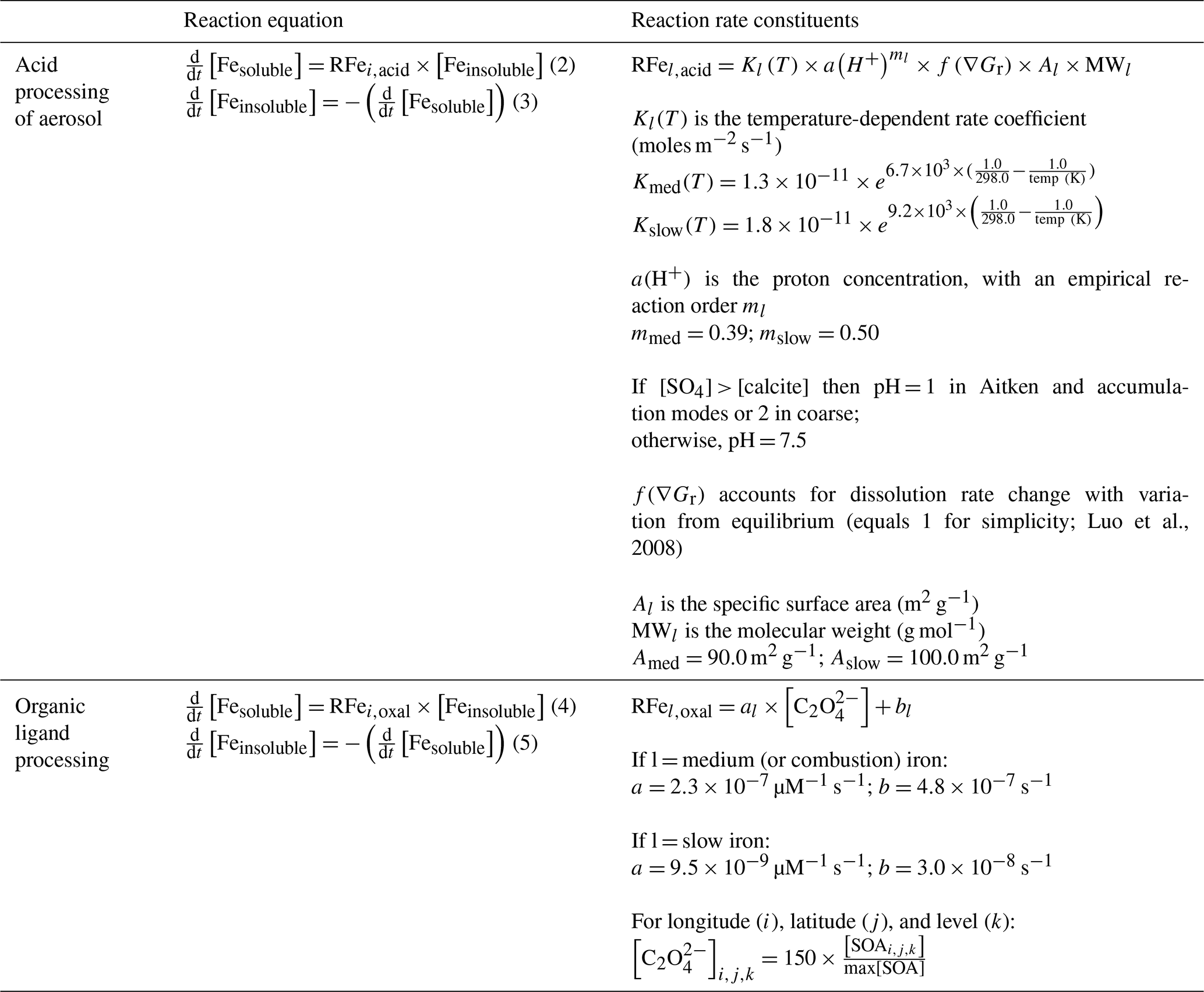
Dust aerosol moving through areas containing acidic gases, with a pH 1–2, increases the solubility of the iron contained within it (Ingall et al., 2018; Longo et al., 2016; Meskhidze et al., 2003; Solmon et al., 2009), and mineralogy is a key factor determining the rate of dissolution at a given pH (Journet et al., 2008; Scanza et al., 2018). Modelled aerosol pH in MIMI was parameterized to depend only on the ratio of the calcium to sulfate aerosol concentration (Scanza et al., 2018). At each time step, if [SO4] > [calcite], then the aerosol was assumed to be acidic with a low pH, while if [SO4] < [calcite], then aerosol was assumed to be well buffered (Böke et al., 1999) and the pH = 7.5. In MIMI, we updated the pH calculation from BAM-Fe in two ways: (1) in BAM-Fe, pH was calculated as the mean across all four size bins (0.1–10 µm), while in MIMI, pH was calculated separately for each interstitial aerosol size mode. (2) Aerosol measurements of pH have shown that interstitial aerosol is likely to be more acidic than was assumed in BAM-Fe (Longo et al., 2016; Weber et al., 2016), even when taking into account declining sulfate levels (Weber et al., 2016); therefore, we have lowered the aerosol pH to 1 (from 2) in both the Aitken and accumulation modes wherein sulfate aerosol dominates. However, in the coarse mode, wherein dust dominates, we retained the lower pH boundary of 2. Furthermore, MAM aerosol was simulated as an internally mixed aerosol; therefore, the SO4 : Ca ratio included the mixing of these aerosol components within each mode. See Sect. 4.2 for a comparison of acid processing in MIMI with the literature and the previous model (BAM-Fe).
All aerosol species in the host CAM5 framework are carried in either an interstitial (i.e. not associated with water) or cloud-borne (i.e. associated with water) phase. The organic ligand reaction only proceeds within MIMI if the condition that cloud is present in the grid cell is first met. If cloud is present then only the iron aerosol which is associated with water undergoes organic ligand processing (i.e. the interstitial aerosol component remains unchanged). Any future development of MIMI within an aerosol model which does not advect a separate tracer for the cloud-borne phase of aerosol would therefore need to adjust the reaction to take account of this. An assumed oxalate concentration in MIMI was estimated based on the modelled organic carbon concentration and could not exceed a maximum concentration threshold of 15 µmol L−1 (Scanza et al., 2018). In BAM-Fe, oxalate was derived from the sum of both the primary and secondary organic carbon aerosol concentrations, while in MIMI this was updated to be dependent only upon the secondary organic carbon source because oxalate is itself a product of the oxidation of volatile organic carbon gases (Myriokefalitakis et al., 2011). An additional term was added to the reaction mechanism to account for the small amount of organic ligand processing proceeding by species other than oxalate (Scanza et al., 2018). See Sect. 4.2 for a comparison of in-cloud organic dissolution in MIMI with the literature and the previous model (BAM-Fe).
2.4.2 Computational costs
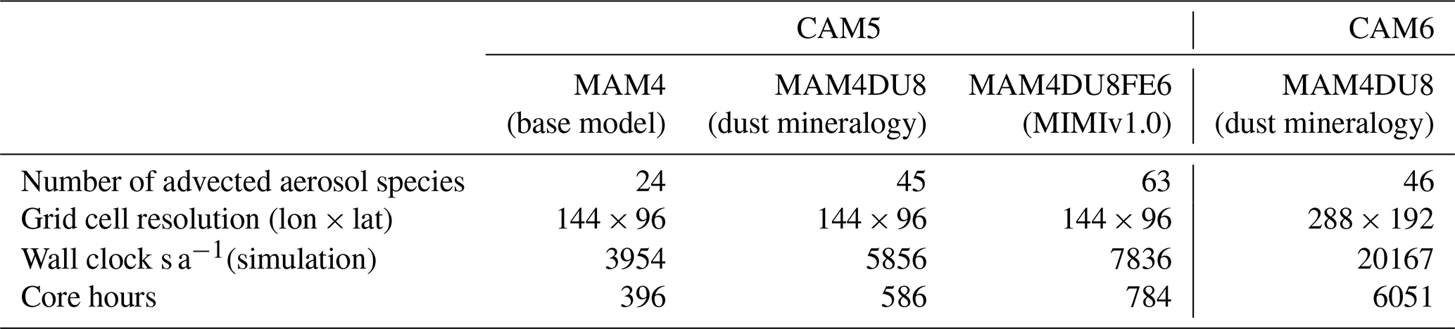
Earth system models are generally characterized by having a heavy computational burden in simulating atmospheric processes. The inclusion of MIMI requires eight dust mineral tracers (a net addition of seven) and six iron tracers. The total number of new aerosol tracers is 39 (13 in each of the three aerosol modes) if dust mineralogy is not already present or 18 new aerosol tracers if it is (e.g. NASA GISS model; Perlwitz et al., 2015a, b). The additional computational cost of MIMI within CESM-CAM5 is approximately a doubling of the required core hours; around half of that is associated with dust mineralogy speciation and the other half with iron speciation and processing (Table 6). Note that additional computational tuning, or changes in configuration, could modify these computational change estimates. For example, with dust mineralogy (MAM4DU8) there is an approximate tenfold increase in required core hours due to model structural differences when transitioning from CAM5 to CAM6.
Table 6Simulation time (in seconds per simulated year) for the CESM-MAM4 model. The CAM5 base model, with the addition of dust mineralogy and with the addition of dust mineralogy and iron processing (i.e. MIMI v1.0), is shown. The cost of running the new higher-resolution CAM6 model with dust mineralogy is also shown for comparison. All CAM5 simulations were executed on 10 nodes with 36 cores per node for 2 years (2006–2007) with consistent output fields. CAM6 simulations are executed on 30 nodes with 36 cores per node.
2.5 Observation and model iron calculations
2.5.1 Spatially aggregating limited observations
The observations of total iron concentrations and the fractional solubility of iron used in this study are joint totals (1524 records) of those reported in Mahowald et al. (2009) and Myriokefalitakis et al. (2018). However, many of these observations represent averages of only one or a few days of iron and soluble iron measurements and can thus be difficult to compare against annual, or longer, mean time periods calculated within the model. Furthermore, building empirical distributions of iron properties from observations requires a larger sample size than currently available in many regions. We therefore tested how aggregating the observations spatially, sometimes termed “super-obbing”, altered our model evaluation. Our objective was to capture the small regional-scale properties of iron and not those at a point source; therefore, we assume that the benefits gained by aggregating in this way, which include helping to produce a statistically useful number of observations, outweigh any potential biases.
2.5.2 Variations in model temporal averaging
The model was run at a 30 min time resolution. At each 30 min time step, soluble iron, total iron, and the ratio of soluble to total iron (iron solubility) were computed. The model output was Si, (daily mean soluble iron concentration on day i), Ti (daily mean total iron concentration on day i), and Ri (daily mean iron solubility on day i). Note that Ri is the daily mean of the calculated 30 min solubilities and hence is not equal to Si∕Ti. We define online solubility as the average of ratios calculated as follows:
where n represents the total number of records over which the average was calculated. Online solubility is reported throughout this study. In Sect. 3.4, we then compare the average of ratios to the ratio of averages (defined as offline solubility), calculated as follows:
where and are the grid cell averages of soluble and total iron concentrations, respectively, over the total time period considered in this study (2007 to 2011). While Eq. (7) is common within the literature, this methodology can produce larger variability in iron solubility across grid cells because it is based on both soluble and total iron annual mean concentrations. In the online method, variability is reduced as extreme values in soluble and total iron concentrations generally do not occur at the same time. We can define the occurrence of extreme values, with respect to the time frame considered, by analysing a relative Z-score metric calculated as follows:
or
where Fe is either total (Fet) or soluble (Fes) iron. The relative normalized Z score can then be calculated as follows:
where Zt,i and Zs,i are the Z scores of total and soluble iron concentrations, respectively, at each grid cell for each time step i. The Z-score metric provides a relative direction and distance of an instantaneous value with respect to its mean. The Z score is reported in multiples of the standard deviation (Eq. 8); therefore, a Z score of zero indicates that the data point value is identical to the mean value. To assess the relative difference in the variability at a given time between the modelled total and soluble iron concentration and its mean, we calculated the difference in Z scores between total and soluble iron concentrations and normalized it using the Z score of total iron concentration (Eq. 9). Note that the Z score of the soluble iron concentration could also be used to normalize the difference. This method allows for the examination of how the occurrence of extreme concentration values in total and soluble iron influences the method of solubility calculation (Eq. 6 vs. Eq. 7).
2.6 Iron ocean deposition source apportionment
An ocean deposition source apportionment sub-study was designed to classify ocean deposition regions according to the dominant atmospheric soluble iron source, rather than ocean basins defined from a more traditional physical oceanographic viewpoint (e.g. Gregg et al., 2003). By incorporating recent model estimates for dust and the importance of pyrogenic iron emissions (Luo et al., 2008; Matsui et al., 2018) the seven large-scale source regions defined in Mahowald et al. (2008) were modified slightly to separate the major dust iron source regions from fire and anthropogenic combustion iron source regions. This resulted in a total of 10 iron emission source regions (Fig. 1; see also Table S1 for details).
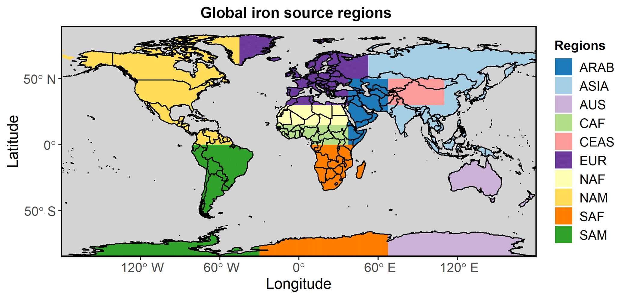
Figure 1Major iron aerosol emission source regions.
Simulations in the source apportionment study used BAM-Fe, as described in Scanza et al. (2018), with slight modification. Briefly, anthropogenic combustion iron emissions were increased by a uniform factor of 5, and iron from fires followed the updated Fe : BC ratio (Table 4) and seasonal variability in the fire BC emissions, all as per MIMI. Aerosols were externally mixed in BAM, and therefore altering the regional aerosol loading did not affect aerosol transport or deposition in the more significant way it could in MAM, in which aerosols are internally mixed. This information was then used in Sect. 4.3 to compare differences in the daily mean deposition of soluble iron between the BAM-Fe and MIMI models within each defined ocean region.
In terms of Earth system modelling and the biogeochemistry that connects the land–atmosphere–ocean components, we are ultimately motivated to improve the magnitude of the atmosphere-to-ocean iron deposition flux and its fractional solubility (from which the soluble iron flux can be derived). We compare the model results with a series of observations and herein highlight some of the problems discovered when directly comparing with a sporadic (in both space and time) observation dataset, as is currently common practice (Myriokefalitakis et al., 2018).
3.1 Global dust comparisons
Comparison of dust AOD with regional dust AOD observations (Fig. 2) from the AERONET observational datasets (Holben et al., 1998), as subsampled in Albani et al. (2014), shows good agreement globally (correlation: r2=0.64). This results in MAM annual global mean emissions of 3250±77 Tg dust a−1 (Aitken 16 Tg a−1, accumulation 36 Tg a−1, coarse 3198 Tg a−1), which is at the higher end of literature estimates of ∼500–4000 Tg dust a−1 (Bullard et al., 2016; Huneeus et al., 2011; Kok et al., 2017). Dust emissions in MAM are 84±4 % higher than our previous mean of 1768 Tg dust a−1 in BAM (Scanza et al., 2018) because dust lifetime has proportionally decreased (Table S2), which affects coarse-mode dust aerosol (wherein 98 %–99 % of total dust mass is emitted) more than fine-mode dust aerosol. Globally, both dust concentrations (correlation: r2=0.89) and deposition (correlation: r2=0.83) are simulated well compared to observations within MIMI. A higher correlation of modelled dust concentrations with observations is calculated in the Northern Hemisphere (NH; r2=0.89) compared to the Southern Hemisphere (SH; r2=0.67), but the gradient of the line of best fit is further from 1 : 1 (NH: 1.22 vs. SH: 1.07). Conversely, for dust deposition a lower correlation with observations is simulated in the NH (r2=0.75) compared to the SH (r2=0.60) but with a gradient of the line of best fit closer to 1 : 1 (NH: 1.07 vs. SH: 0.72). Overall, the results presented in this study suggest an improvement on previous dust modelling complications related to underestimating dust deposition when tuned to dust concentration (Huneeus et al., 2011).
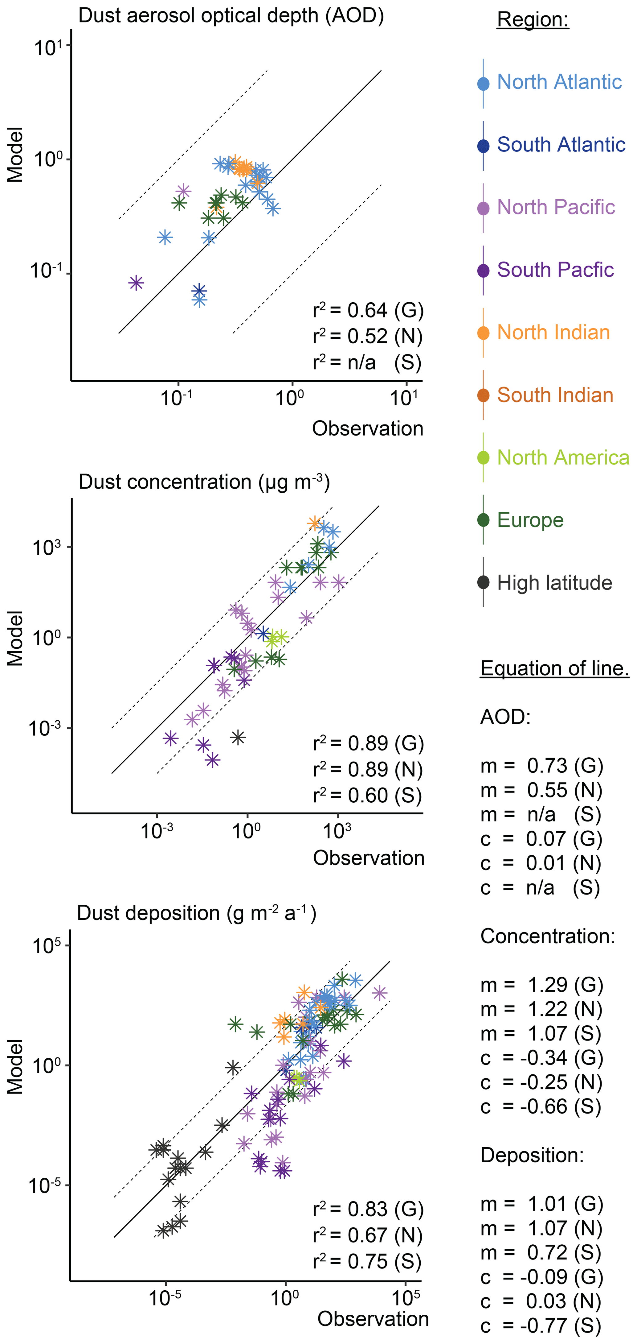
Figure 2Dust aerosol optical depth, surface concentrations, and deposition in modal aerosol model and observations (Albani et al., 2014; Holben et al., 1998). Correlation (r2), gradient (m), and intercept (c) shown for global (G), Northern Hemisphere (N), and Southern Hemisphere (S) regions.
3.2 High-latitude dust and iron aerosol
Including the parametrization of Kok et al. (2014a) removes the requirement of a soil erodibility map (Table 1). In addition, in previous versions of the model, high-latitude dust sources were zeroed because there were no observations at that time to support high-latitude sources of dust (Albani et al., 2014). However, more recent observations have suggested that high-latitude dust sources do exist (Bullard et al., 2016; Crusius et al., 2011; Tobo et al., 2019), often related to glacial processes (Bullard, 2017) with a higher fraction of bioavailable iron relative to lower-latitude dust sources (Shoenfelt et al., 2017). Thus, for the new version of the model we have allowed for the inclusion of high-latitude dust sources (Fig. 3). In general, aerosol dust and iron concentrations peak closest to the coastlines and during summer. Emissions of dust from >50∘ N are % of the global dust total, which is half of the estimates derived from field and satellite data at 2 %–3 % of the global total (Bullard, 2017; Bullard et al., 2016). However, the resulting magnitude and seasonality of dust concentrations have been shown in a recent study to be consistent with observed measurements from Svalbard (Tobo et al., 2019).
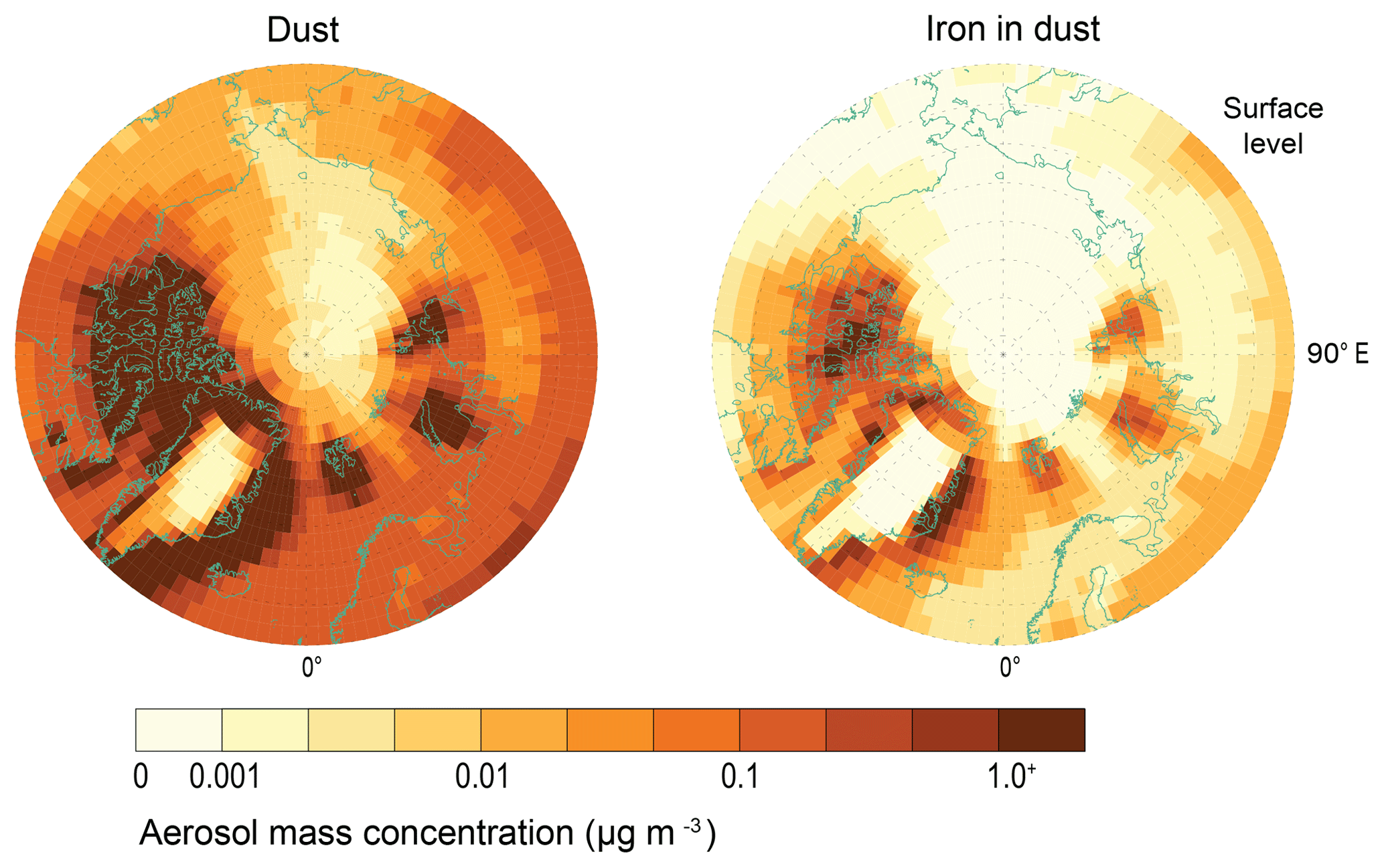
Figure 3High-latitude (>60∘ N) dust (sum of eight mineral species and four dust–iron species) and iron (sum of four dust–iron species) mass concentrations (µg m−3) at the surface model level.
3.3 Global iron aerosol concentration and fractional solubility
There are several propositions explaining sources of soluble iron and the inverse relationship between total iron amount and iron solubility (Sholkovitz et al., 2012). While total iron mass concentrations are dominated by desert dust sources, soluble iron can be a product of mineral dust processed in the atmosphere or emitted from pyrogenic sources (Chuang et al., 2005; Guieu et al., 2005; Ito et al., 2019; Luo et al., 2008; Meskhidze et al., 2003; Schroth et al., 2009). Previous studies have shown that either of these can explain the inverse relationship and that the spatial distribution of data is required to provide more information (Mahowald et al., 2018). Therefore, we explored how to best use the spatial data to compare with the model results. The 5-year (2007 to 2011) mean iron concentration from MIMI is compared to an extensive dataset of observations of total iron and its fractional solubility (Fig. 4). The model captures the global mean observational total iron concentration well; however, relatively low regional correlations (r2<0.4) occur in the south Indian (r2=0.0), South Atlantic (r2=0.34), North American (r2=0.35), and high-latitude (r2=0.06) ocean regions, suggesting that future model improvements can be focused here.
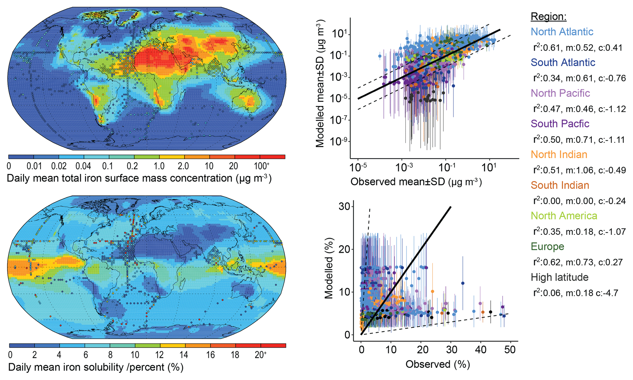
Figure 4Daily mean model total iron concentration and solubility from 2007 to 2011. Observations (circles) overlaid (at resolution of the model grid) as a mean from 1524 individual records in Mahowald et al. (2009) and in Myriokefalitakis et al. (2018). Also shown are scatter plots of the model mean and standard deviation compared to each available observation and identified by oceanic region. Correlation (r2), gradient (m), and intercept (c) for total iron with observations shown for each region.
In the absence of iron atmospheric process modelling, ocean biogeochemistry models with an iron component (e.g. Aumont et al., 2015; Moore et al., 2004) have estimated iron solubility from offline dust modelling by means of an assumption that it contains 3.5 % iron by weight, of which 2 % is soluble. Iron solubility is highly temporally and spatially variable, however, and in the absence of spatial atmospheric emission information, pyrogenic iron sources, and atmospheric processing of iron, an estimate of 2 % solubility leads to underestimates of observed iron solubility in nearly all HNLC ocean regions (Fig. 4).
Aggregating observations onto a lower-resolution grid (sometimes termed super-obbing) compared with the model can help reduce the representation error when comparing with such limited observations (Schutgens et al., 2017). Fig. 5 uses an observational resolution one-third that of the model, and the model-to-observation comparison of the mean state is thus improved. Persistent observation-based features of the local environment become more obvious, while less frequent ones conversely diminish. At this observational resolution, the low total iron concentrations in the North Atlantic ∼30∘ N, as seen in Fig. 4, are perhaps not a common feature, and the model much more precisely represents the climatological state here than Fig. 4 might suggest. However, examining the North Pacific reveals that the model imprecisely represents the mean state here. Potential missing iron sources in remote regions, such as the North Pacific, include the following: (1) shipping emissions (Ito, 2013), which have a high soluble iron content from oil combustion (Schroth et al., 2009); (2) volcanic emissions, which provide a localized “fertilizer” to the surface ocean owing to the macronutrients and trace metal nutrients contained within them (Achterberg et al., 2013; Langmann et al., 2010; Rogan et al., 2016); and (3) low Asian and South American aerosol concentrations, either through underrepresenting combustion emission sources (Matsui et al., 2018) or in the transport and deposition of aerosol within these regions (Wu et al., 2018). These are discussed in more detail in Sect. 5.1 and 5.2.
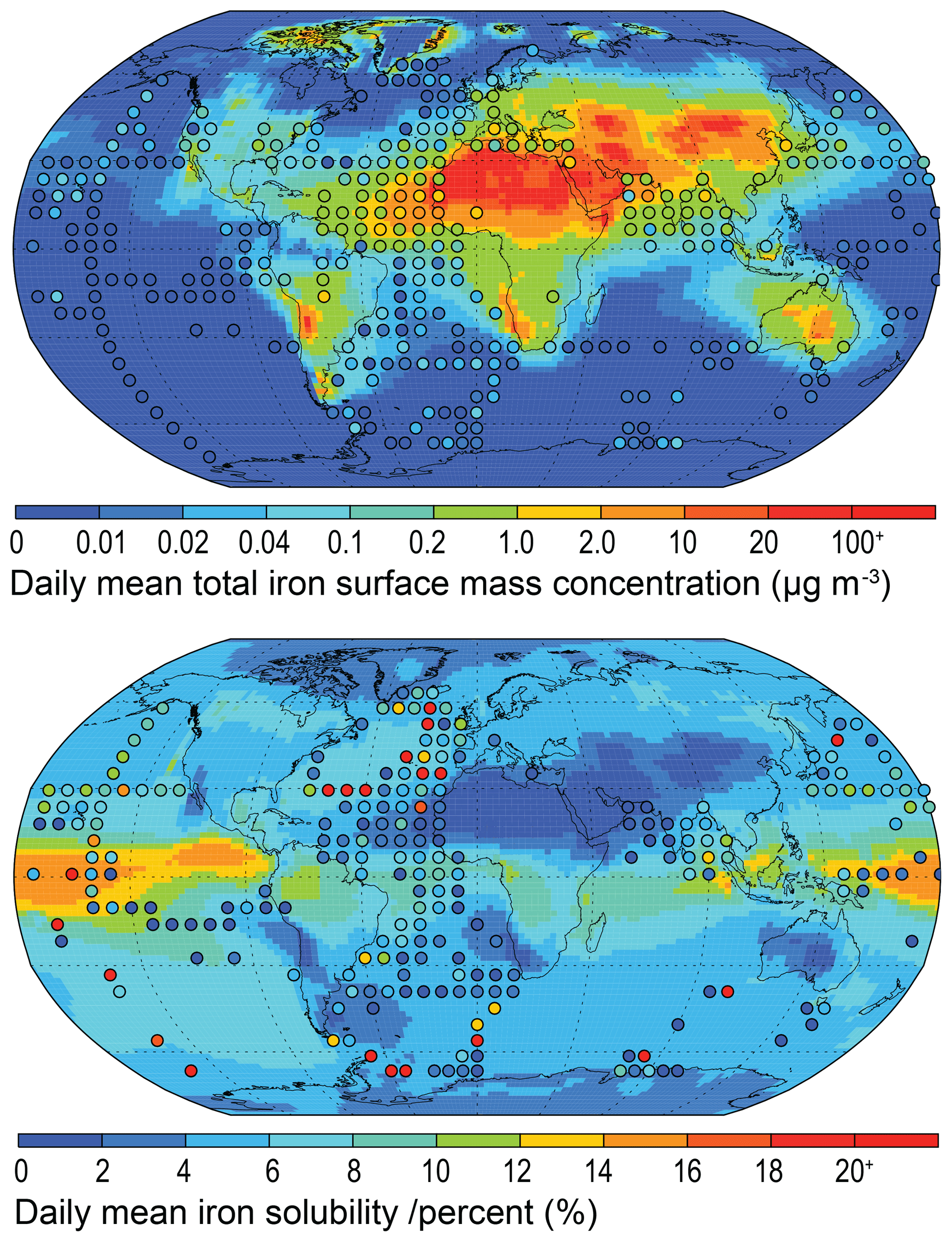
Figure 5Daily mean model total iron concentration and solubility from 2007 to 2011. Observations (circles) overlaid (at a resolution one-third of the model grid) as a mean from 1524 individual records in Mahowald et al. (2009) and in Myriokefalitakis et al. (2018).
In terms of iron solubility (soluble iron concentration ∕ total iron concentration), the model is not capturing the observational mean state in many regions (Fig. 5). A detailed examination of the observation point at 18∘ N and 330∘ E (anomalous green point surrounded by blue points in the North African outflow plume in Fig. 4) and the nine model grid cells co-located with it in Fig. 6 shows how a single high observation (155 % percent solubility) is causing a representation issue (see also Sect. 4.3 regarding soluble iron deposition). Both model and observation histogram distributions are similar, as are the median (model: 1.8, observation: 0.9) and geometric mean (model: 2.1, observation: 1.3) values. However, the arithmetic means are not similar (model: 2.5, observation: 9.6) and while a high observation value of 155 % is likely to be an outlier and should be at most 100 %, it still informs us about what is possible, and simply discounting it (even at an adjusted 100 %) would require strong justification. It is therefore advisable to instead alter the estimator of the average. Comparing model to observation differences calculated using the median or geometric mean reveals that they are similar in magnitude, as one would expect for log-normally distributed data (Fig. 6 insert). Although the median is robust with respect to outliers, the model results may not exhibit a uniform Gaussian distribution (Fig. 6 insert; solid compared to dashed lines), and often the number of available observations is also low (Fig. 7), suggesting that its use also requires careful consideration. An equivalent methodology to the geometric mean in Fig. 7 would be to first log transform the data before calculating the arithmetic mean. Arguments pertaining to the appropriate methodology for comparing model results to temporally limited observations extend beyond the iron aerosol examination in this study to all aerosol comparisons with limited observations.
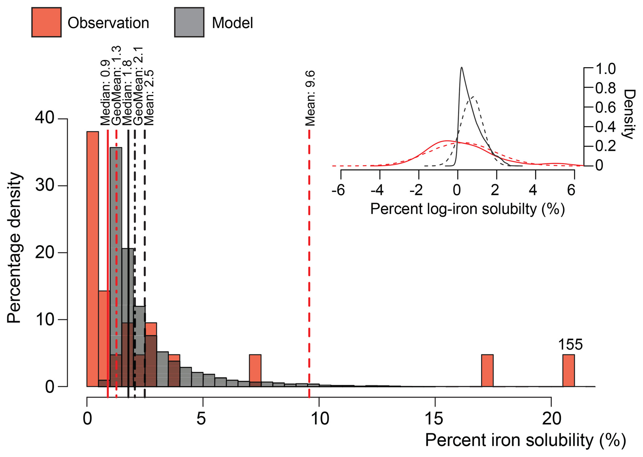
Figure 6Histogram of observations (n=21) and daily model results (2007 to 2011) of iron solubility between 16 to 20∘ N and 27 to 32∘ W (one observation point and nine co-located model grid cells in Fig. 5). Mean (dashed lines), geometric mean (dot-dash lines), and median (full line) values shown the above respective dataset colour line. Note that the single observation value of 155 % is off the scale and placed as such with the value given above. Insert: log plot for the same data (solid lines) with projected log-normal distribution from the mean and standard deviation of the data (dashed lines).
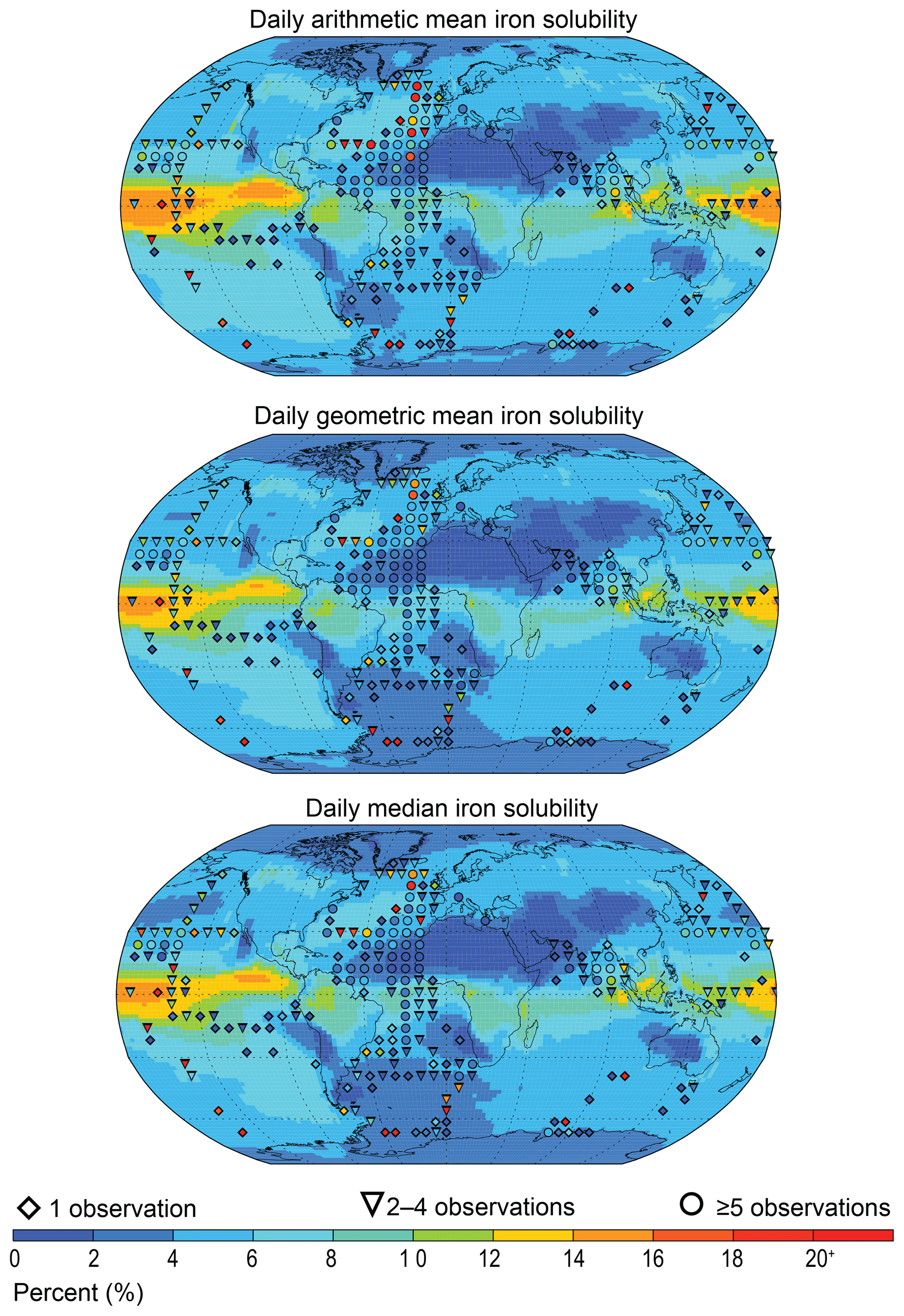
Figure 7Daily arithmetic mean, geometric mean, and median model solubility (2007 to 2011). Observations are overlaid (at resolution one-third of the model grid) as the arithmetic mean, geometric mean, or median with respect to the model averaging. The number of observations is denoted by symbols: lowest confidence (one observation, diamond); intermediate confidence (two to four observations, triangle); highest confidence (five or more observations, circle).
3.4 Calculating iron solubility
It is interesting to note the effect that the order of operations (taking the average of ratios compared to the ratio of averages) has when calculating iron solubility (Fig. 8). Throughout this study, the percent of iron solubility was calculated at each model time step (30 min) and then the daily mean output was analysed (online; Eq. 6) at an annual or 5-year mean time resolution. It is also acceptable to use the simulated soluble and total iron concentrations to generate the annual or 5-year mean iron solubility in a post-processing step (offline; Eq. 7). The resulting differences between methods are not insignificant (Fig. 8); however, the offline method creates a distribution in which low iron solubility is generally lower and the highest (>18 %) iron solubilities are generally higher. Overall, the global annual mean iron solubility calculated online is one-third (34 %; NH = 40 %, SH = 29 %) higher than when calculated offline.
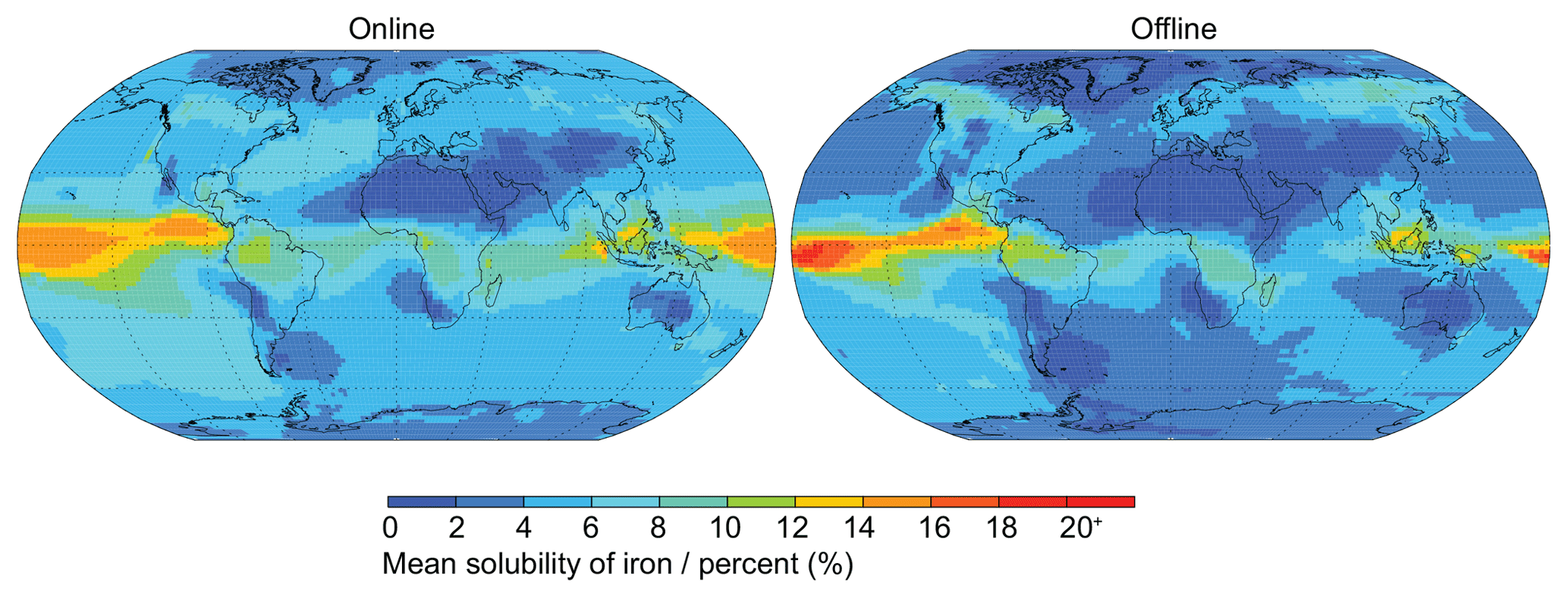
Figure 8Mean solubility of iron when solubility is calculated at each 30 min model time step (“online”) and when it is calculated from the post-processing of daily mean soluble and total iron concentration (“offline”).
The average relative Z score (Eqs. 8 and 9) is around zero for most model grid cells (Fig. 9), indicating that they mostly followed similar temporal and relative magnitude trends. However, even if the average relative Z scores are around zero and the ratio of relative standard deviations is around one, the ratio of online- to offline-calculated iron solubility is most likely >1. Temporal differences in the soluble and total iron concentration might therefore be controlling the overall solubility at each model grid cell. We also find that the ratio of online and offline solubility is >1 for most of the cases when the ratio of the relative standard deviations of soluble and total iron is <1 (Fig. S2), indicating that the differences in both methods of iron solubility calculation are sensitive to the differences in the relative size of the tails of the distribution. That is, if soluble iron has narrower tails compared to total iron at any grid cell, it is highly likely that a higher solubility will be obtained in the online method compared to offline. The extreme ratio of the tails of soluble and total iron is only found in specific regions with the highest temporal variability in emissions and modelled solubilization of insoluble iron (Fig. S2).
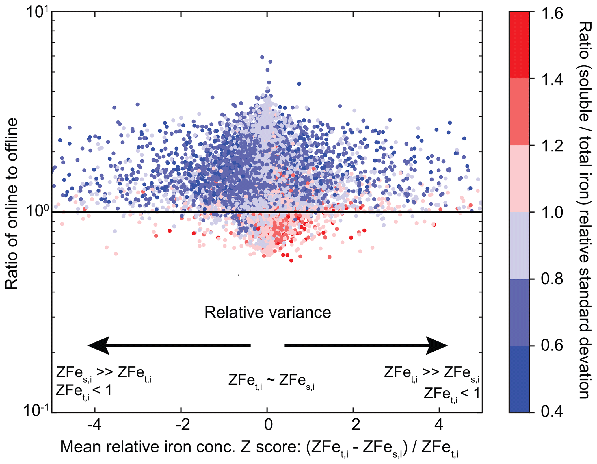
Figure 9Relationship of online- to offline-derived iron solubility to the relative Z score for total (ZFet) and soluble (ZFes) iron and the relative standard deviation () at each grid cell for the year 2007.
Field measurements have generally suggested an inverse relationship between total and soluble iron concentrations (Myriokefalitakis et al., 2018). This means that high total iron concentrations are generally accompanied by low soluble iron concentrations and vice versa. By assuming that the field measurements faithfully represented the actual average values of soluble and total iron concentration at those locations, we implicitly assume that all the measurements have a Z score of zero. In Fig. 9 we show that this is not the case with the modelled results, and the two variables can be relatively farther from their respective means even when averaged over the modelled time period.
The sensitivity of a result to the order of operations extends beyond iron solubility to any variable that is calculated in a similar manner, and current multi-model intercomparison project (MIP) protocols do not explicitly account for this. However, the effects of outliers, in both online and offline methods, can be reduced by employing the geometric mean and has been used in some MIPs (e.g. Mann et al., 2014). It will also be important to consider differences in the solubility of iron induced by the choice of the order of operations as ocean biogeochemical models move away from using offline results from global climate or chemistry transport models to online results within Earth system models, which are designed to couple the two components at each time step. For short-term interactions between deposited iron and ocean biota, shorter-term averaging may be more important (e.g. Guieu et al., 2014), but for the long-term accumulation of iron that is (re)cycling in the oceans, the longer-term average may be more appropriate (Moore et al., 2013). One should be aware, however, that iron is readily removed from the ocean mixed layer, and thus the lifetime of iron may well be short enough for the online calculation to be more appropriate much of the time (Guieu et al., 2014).
In this section, we discuss how the new modal aerosol-mode version of MIMI compares to its predecessor bulk aerosol model version (BAM-Fe) throughout all three stages of the atmospheric iron life cycle.
4.1 Iron emission comparison
Globally averaged emissions of dust (3200 Tg a−1) and its iron component (126 Tg a−1) are within the current multi-model range (Table 7). The simulated annual mean iron in dust percentage is 4.1 %, with the highest percent occurring in the coarse mode at 6.5 % and the lowest percent occurring in the Aitken mode at 1.1 %. Accounting for dust mineralogy therefore increases the global mean iron percent by weight above the currently well-used global mean estimate of 3.5 % (e.g. Jickells et al., 2005; Shi et al., 2012).
Table 7Dust, fire, and anthropogenic combustion emissions of iron and relevant co-emitted aerosol emissions (to two significant figures). Multi-model emission range from the four global atmospheric iron models (including BAM-Fe) reported in Myriokefalitakis et al. (2018). Fine (sum of Aitken and accumulation modes) and coarse (coarse mode) mass emissions also given for dust, fire iron, and combustion iron.
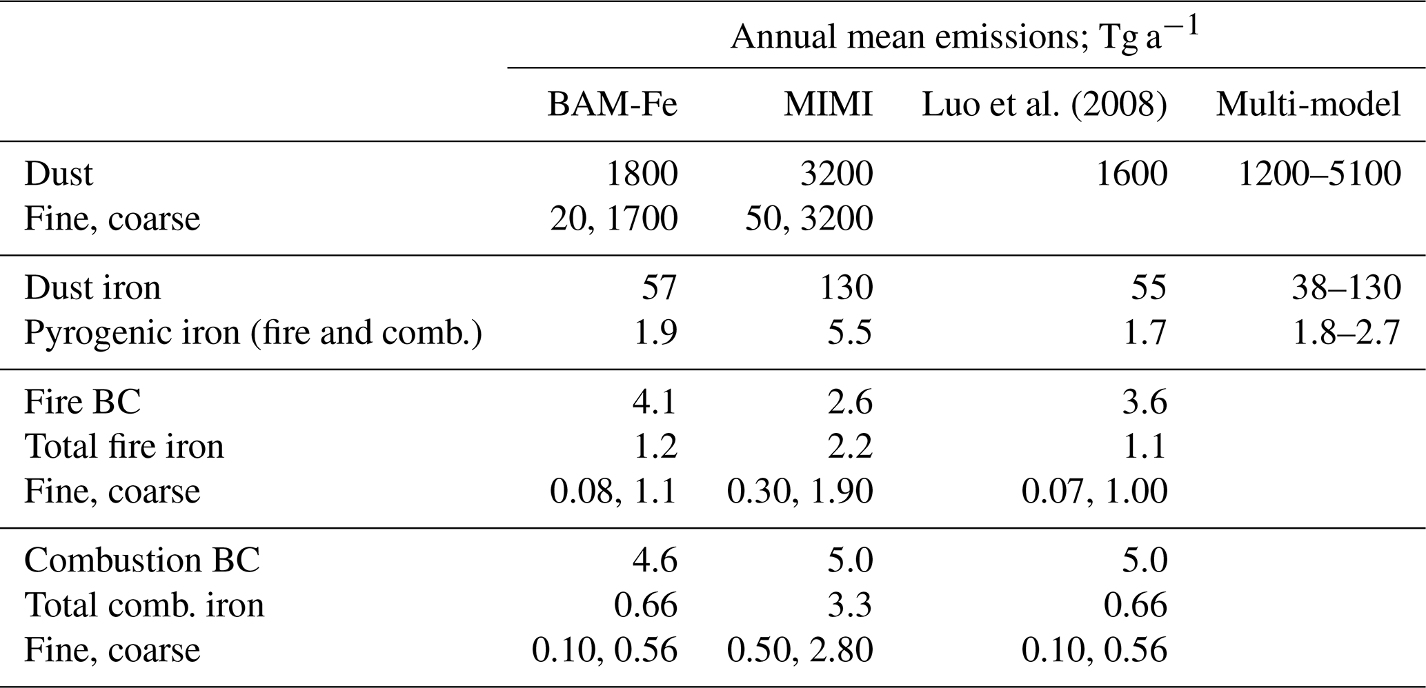
Compared to BAM-Fe, MIMI dust emissions are ∼80 % higher and the iron it contains is ∼120 % higher (Table 7). Although both the BAM-Fe and MIMI models are globally tuned to a similar dust AOD (∼0.03) and based within the same host model (CESM), changing from a bulk aerosol scheme (e.g. Albani et al., 2014; Scanza et al., 2015) to a modal aerosol scheme reduces the aerosol lifetime significantly (Liu et al., 2012 and Table S2). The spatial distribution of dust emissions is also different following the move to the Kok et al. (2014a, b) parameterization (Table 1), resulting in the spatial distribution of dust AOD also being altered (Fig. S3). Total pyrogenic iron emissions (sum of fires and anthropogenic combustion activity) in MIMI are higher than previous estimates by a factor of between 2 and 3 (Table 7), reflecting the growing evidence that they have been previously underestimated (Conway et al., 2019; Ito et al., 2019; Matsui et al., 2018).
4.2 Iron atmospheric processing comparison
There is a much lower aerosol pH in the fine aerosol modes (Aitken and accumulation) in MIMI compared to that in BAM-Fe (Fig. 10). This is due to a combination of resolving pH in each aerosol size mode in MIMI and the subsequent lowering of the pH value (1) being applied in the two fine aerosol modes (Aitken and accumulation). Conversely, dust dominating the coarse aerosol mode provides more of an opportunity for [calcite] > [SO4] in this aerosol size fraction, resulting in most continental areas having a high coarse-mode aerosol pH in MIMI compared with the higher pH being much more localized to the major desert regions in BAM-Fe. Acidic processing of iron in MIMI therefore proceeds faster globally in the fine-sized aerosol modes (Aitken and accumulation) compared to the BAM-Fe fine-sized bin (0.1–1 µm), but it is generally slower over continental regions in the coarse mode than in BAM-Fe coarse-sized bins (1–10 µm).
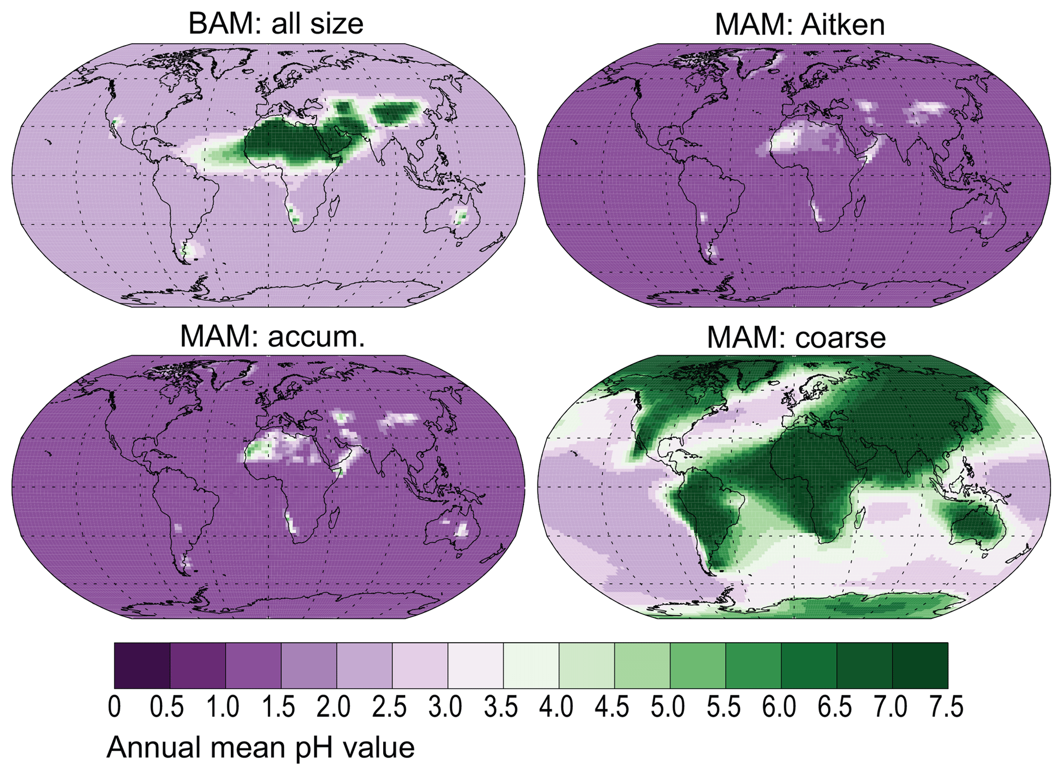
Figure 10Surface-level annual mean interstitial aerosol pH. If [SO4] > [calcite] then pH = 1 in Aitken and accumulation modes or 2 in coarse; otherwise, pH = 7.5 (Table 5).
Comparison of Fig. 10 to modelled pH estimates by Myriokefalitakis et al. (2015) shows generally good agreement in the NH, but in the SH MIMI simulates less acidic coarse-mode aerosol over continental regions and more acidic aerosol over marine regions. As iron models are unable to capture the high observed iron solubility (>10 %) over SH marine regions (Myriokefalitakis et al., 2018) and in the absence of remote pH aerosol observations, we suggest that our basic parameterization captures an aerosol pH which is suitable for use in Earth system models

Figure 11(a) Relative difference in organic ligand reaction on in-cloud iron aerosol dissolution between MIMI and BAM-Fe. Due to significant differences in simulated cloud cover between CAM4 and CAM5 oxalate concentrations [OXL] are multiplied by the model-simulated cloud fraction in this figure. (b) Surface-level oxalate (OXL) concentration in the model and observations. Model values are monthly mean (2007–2011) and annual standard deviation. Observation values are from Table S3 in Myriokefalitakis et al. (2011) and reported with uncertainty where given.
Model physics, and hence simulated cloud cover, are significantly different between CAM4 and CAM5. Figure 11a shows the relative model difference in the oxalate distribution between MIMI, which also includes an increase in the tuning factor by an order of magnitude (from 15 to 150; Table 5), and BAM-Fe by normalizing by the simulated cloud fraction in each model. The effect of oxalate on iron dissolution is therefore larger in MIMI over extratropical ocean regions, where iron models underrepresent solubility (Myriokefalitakis et al., 2018), and land regions which are dense in tropical vegetation or industry (both centres of large aerosol precursor gas emissions). Compared to observations (Myriokefalitakis et al., 2011; Table S3) modelled oxalate concentrations are well represented at high observed concentrations but are biased low when observed concentrations are low (Fig. 11b). The low model bias is stronger within remote observational regions (marine vs. urban observation sites), suggesting that the removal of secondary organic aerosol may be too strong within the model and/or that there is a missing marine aerosol precursor gas emission source (Facchini et al., 2008; O'Dowd and de Leeuw, 2007) in this model which significantly lowers simulated secondary organic aerosol, and thus oxalate, concentrations.
Comparison of mineral dust and pyrogenic sources of modelled soluble iron (sum of emissions and atmospheric dissolution; Fig. 12) with the four iron models (including BAM-Fe) reported by Myriokefalitakis et al. (2018) shows that the spatial distribution in MIMI is broadly similar for most regions of the world. A notable difference exists in the North Pacific region, where the soluble iron source in MIMI is lower than all other iron models, similar to total iron concentrations when compared to observations (Figs. 4 and 5). Future development of MIMI should thus be focused on the North Pacific, including the addition of shipping soluble iron emissions, which are relatively concentrated in this region (Ito, 2013). An improvement for MIMI can be seen over the Atlantic region directly downwind of Saharan soluble iron sources. In general, iron models are overrepresenting iron solubility close to dust sources compared to observations (Myriokefalitakis et al., 2018), and in order for BAM-Fe to reach better agreement with observed iron solubility in this region dust emissions of soluble iron had to be scaled downwards (Conway et al., 2019). We suggest that this improvement is linked to the improved modal representation of aerosol pH in MIMI (Fig. 10).
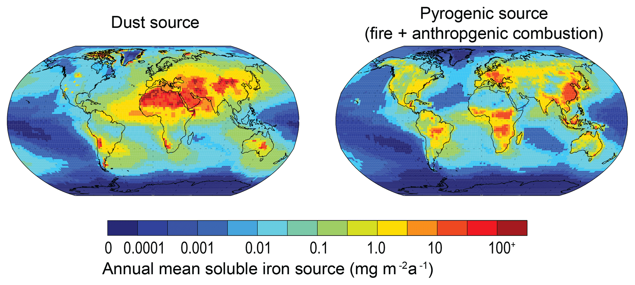
Figure 12Annual mean dust and pyrogenic (sum of fires and anthropogenic combustion) soluble iron source (i.e. sum of emissions and atmospheric processing).
4.3 Iron ocean deposition flux comparison
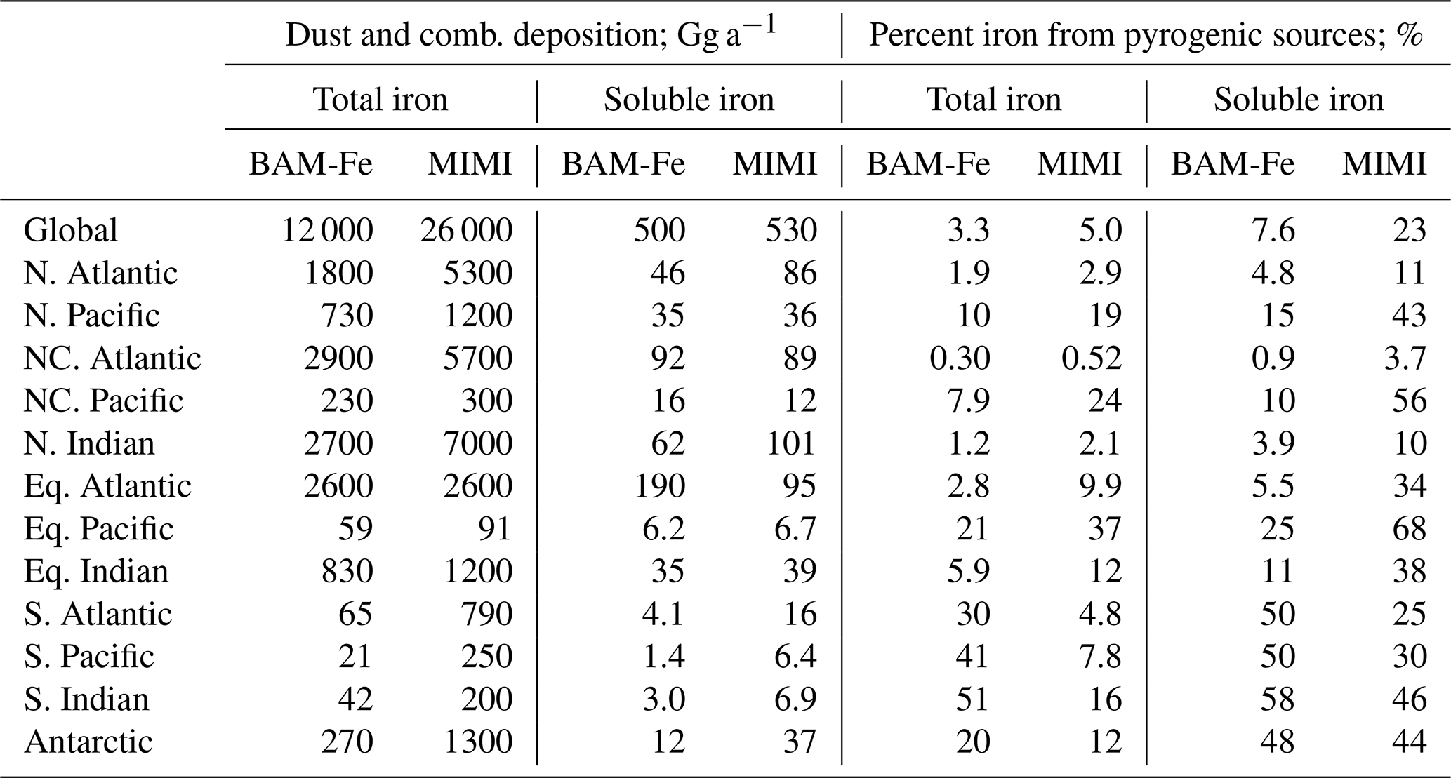
Similar to the previous study by Scanza et al. (2018), we report the amount of total and soluble iron deposited in each of the major ocean basins (Table 8) as defined by Gregg et al. (2003). We find that in MIMI the amount of total iron deposited to all ocean basins is approximately double that estimated in BAM-Fe (26 vs. 12 Tg Fe a−1, respectively), while soluble iron deposition is similar (∼ 0.5 Tg Fe a−1 in both models). The larger mineral dust emission flux in MIMI (3200 Tg dust a−1 compared to BAM-Fe dust emissions of 1800 Tg dust a−1) is driving most of the increases in total iron deposition because it is the primary iron source (Table 7). In general, the magnitude of soluble iron deposition to the oceans is more evenly distributed across hemispheres in MIMI owing to a major reduction (approximately one-half) in the equatorial north–central Atlantic basin deposition flux and increases to SH ocean deposition fluxes of a factor of 2 to 4. In MAM4 dust is treated as internally mixed aerosol with sea salt, leading to higher rates of wet deposition than when dust is externally mixed aerosol (Liu et al., 2012) as it is in CAM4. The internally mixed treatment of dust aerosol in MAM4 is thus an important factor leading to the lower simulated dust lifetime when compared to BAM-Fe (Table S2). Over the north–central Atlantic region, the combination of a lower soluble iron source (Fig. 12 compared to Fig. S4b by Myriokefalitakis et al., 2018), dust atmospheric lifetime (Table S2), lower aerosol pH (Fig. 10), and lower relative organic ligand processing (Fig. 11) will all work towards reducing the magnitude of atmospheric soluble iron deposition flux in MAM4 compared to BAM-Fe. There are significant increases in anthropogenic combustion iron deposition in all equatorial and NH ocean basins driven by the fivefold increase in combustion emissions implemented in MIMI. The percent contribution from pyrogenic iron to total iron deposition between MIMI and BAM-Fe is, however, more similar for all northern and equatorial oceanic regions than southern oceanic regions. Beyond the correction to anthropogenic combustion emissions, which are NH dominated, this could be due to differences in the emissions of both dust and fire aerosol, structural differences between models relating to the aerosol size and composition, which alters aerosol deposition rates, or a lower soluble iron source (Fig. 12); it is most likely to be a combination of all three.
Table 8Global and regional ocean basin deposition (Gg a−1) of total and soluble iron in BAM-Fe (Scanza et al., 2018) and MIMI (this study). Deposition was multiplied by the ocean fraction of model grid cells and is reported at two significant figures. The percent contribution from pyrogenic (sum of fires and anthropogenic combustion) iron sources to deposition is also given. Ocean basins are those defined by Gregg et al. (2003) and previously used by Scanza et al. (2018).
The fraction of fire aerosol which is injected above the boundary layer is crucial for determining its capacity for long-range transport (e.g. Turquety et al., 2007). Vertically distributing fire iron emissions in MIMI, as compared to emitting all iron from fires at the surface as in BAM-Fe, increases the long-range transport of iron aerosol to remote ocean regions (Fig. 13). In general, vertically distributing fire emissions results in small increases in soluble iron deposition (between 0 % and 20 %) in SH ocean regions and a larger increase (between 20 % and 40 %) in NH oceans, with converse lower land deposition close to the major regions of fire activity. The exception is in the sub-Arctic North Pacific, an HNLC region, where iron deposition from fires significantly increased until it was more than double that when surface fire emissions are used.
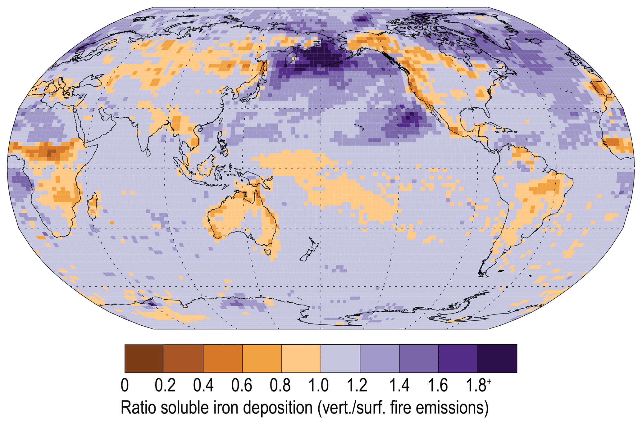
Figure 13The ratio of soluble iron deposition from fires when emissions are emitted with a vertical distribution to fires when emissions are only at the surface (i.e. vertical ∕ surface). Single year (2007) comparison only.
The dry deposition flux is sensitive to aerosol properties, surface roughness, and modelled turbulence. Although increasing the vertical resolution has been shown to increase surface PM10 concentration (Menut et al., 2013) and better simulate the dust vertical profile (Teixeira et al., 2016), it is not yet clear if this would correspondingly increase the dry deposition flux.
Source region comparison
The eight regions in Fig. 14 are chosen based on 10 (one for each region in Fig. 1) simulations undertaken using the modified version of BAM-Fe described in Sect. 2.6. The emission region (Fig. 1) with the highest fractional contribution to the total soluble deposition flux in each grid cell was examined, and from this the boundaries of each region in Fig. 14 were delineated. The resulting eight ocean iron deposition regions are split equally into four in the NH and four in the SH. Note, however, that the NH–SH divide sits at 15∘ S and not the Equator, which is due to transport differences in each hemisphere and the position of the Intertropical Convergence Zone. Of the four regions that can be defined as major dust deposition receptors (Fig. 14; bottom panel bar chart), the north Indian Ocean (no. 1), North Atlantic and central Pacific (no. 4), and South American dust (no. 7) regions have a single dominant source each, while the North Pacific (no. 3) region is more variable. These dust-dominated iron deposition regions are similarly reproduced by other global iron models (Ito et al., 2019; Myriokefalitakis et al., 2018). The regions of the mixed Southern Hemisphere oceans (no. 5) and Australian and South Pacific (no. 6) receive similar amounts of mineral dust and pyrogenic iron, suggesting that the iron sources are spatially closer and thus share much more similar transport pathways than the South East Asian ocean (no. 2) and South American pyrogenic (no. 8) regions, which have a much more distinct pyrogenic iron source signal. Deposition regions are more clearly defined when using this methodology compared to those from a more traditional classification of ocean basins based on physio-geographical oceanography (Fig. S4). This information can be used to assess which ocean regions are most likely to be affected by anthropogenic perturbations to the magnitude of iron sources within different regions, whether through land use, land cover change, or industrialization.
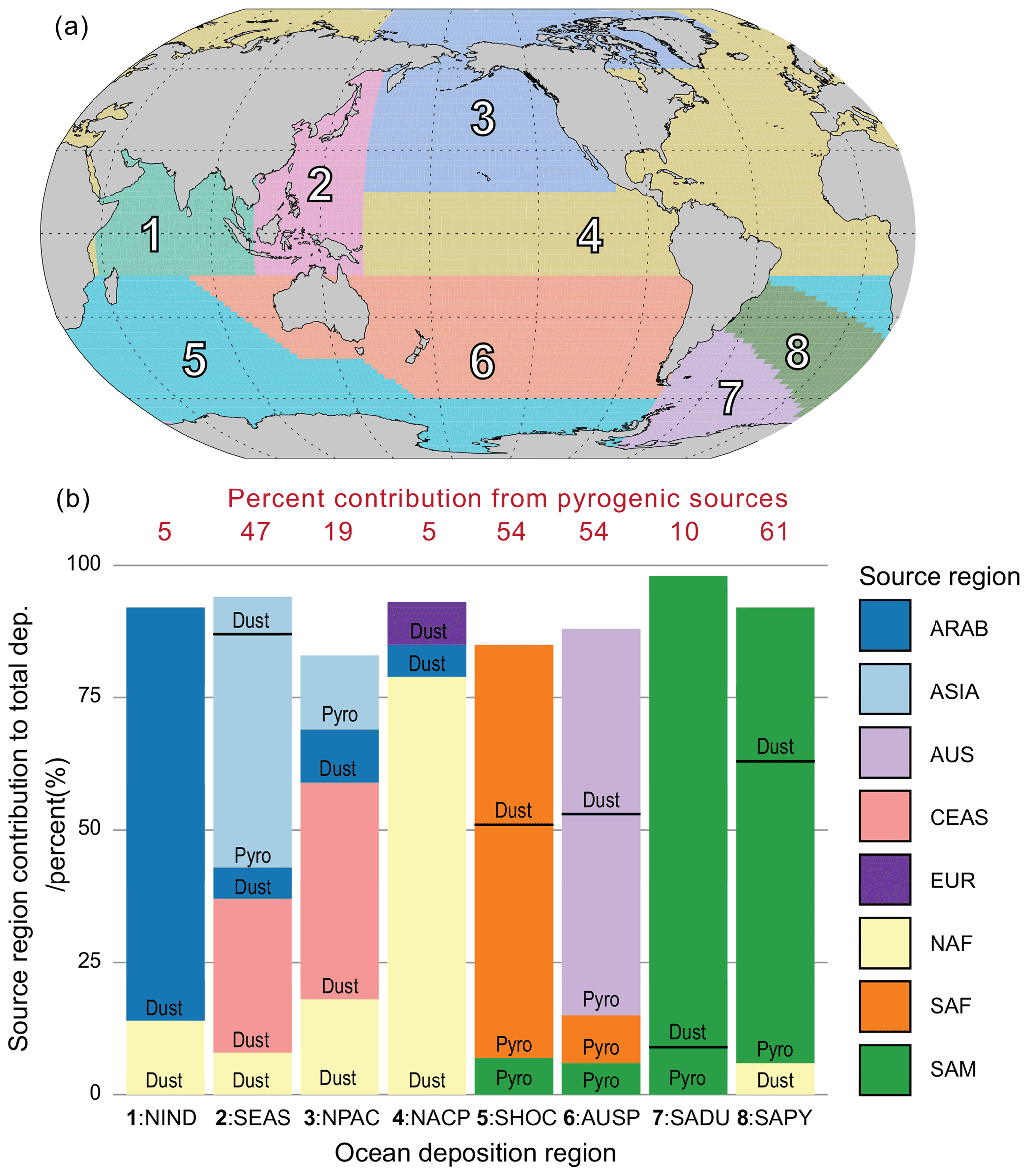
Figure 14(a) Eight soluble iron ocean deposition regions defined by dominant source region apportionment. Region 1: north Indian Ocean (NIND). Region 2: South East Asian ocean (SEAS). Region 3: North Pacific (NPAC). Region 4: North Atlantic and central Pacific (NACP). Region 5: Southern Hemisphere oceans (SHOC). Region 6: Australian and southern Pacific (AUSP). Region 7: South American dust (SADU). Region 8: South American pyrogenic (SAPY). (b) Contribution of each emission source region (Fig. 1) to the total iron deposition across the region. Contributions of dust and pyrogenic (sum of fires and anthropogenic combustion) iron from the source region are also shown. Regions contributing <5 % are filtered out.
The variability in the daily soluble iron deposition flux to each of the eight ocean regions, as seen in Fig. 14, is much larger in MIMI than it is in BAM-Fe (Fig. 15), reaching over 10 orders of magnitude between the minimum and maximum flux in many regions. This is due in part to the increased variability in fire emissions, which was improved in MIMI to track the BC emitted from fires, and switching from the offline soil erodibility map used in BAM-Fe to the Kok et al. (2014a) physically based emission parametrization used in MIMI. Anthropogenic combustion emissions are temporally static in both model frameworks and therefore do not affect the variability in this study as much as fires and mineral dust but will in the future if this is changed to represent a seasonal emission cycle. We can see that each of the dust and fire updates in MIMI have a large impact by comparing the Patagonian dust-dominated South American dust (SADU) region and the fire-dominated South American pyrogenic (SAPY) region. Most of the dust deposited (30 % to 90 %) in the ocean occurs during large dust events that are on just 5 % of the days (Mahowald et al., 2009), resulting in large differences between median and mean deposition amounts in all regions, as seen in Fig. 15. It is important to note that the mean is always above the interquartile range, further supporting our previous arguments pertaining to the modelled mean not being an ideal estimate of the average as it does not represent the log-normal distribution of aerosol. Comparing the mean-to-median ratio suggests that extreme dust events are also more pronounced in MIMI (CAM5) than in BAM-Fe (CAM4).
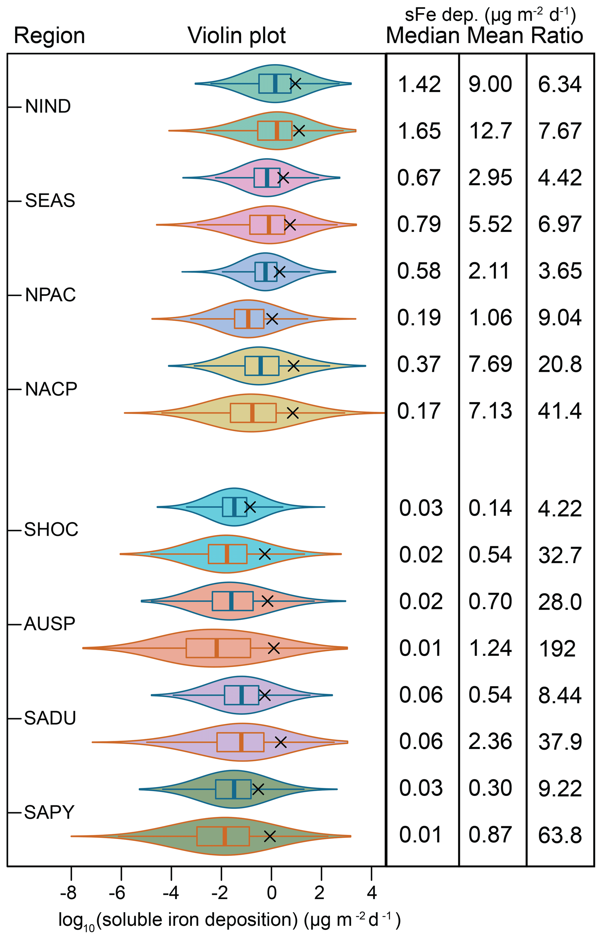
Figure 15Violin plots of 5 years of log10 daily soluble iron deposition (µg m−2 d−1) within each grid cell for the eight ocean regions defined in Fig. 14. Only grid cells in which ocean fraction >0.5 are included in the analysis. Violin colour matches Fig. 1 region colour: north Indian Ocean (NIND); South East Asian ocean (SEAS); North Pacific (NPAC); North Atlantic and central Pacific (NACP); Southern Hemisphere oceans (SHOC); Australian and southern Pacific (AUSP); South American dust (SADU); South American pyrogenic (SAPY). Violin outline colours: blue lines: BAM results, orange lines: MAM results. Black cross: log10 mean daily soluble iron deposition. Median, mean, and ratio (mean ∕ median) values for all 5 years of daily deposition amounts across each basin are also given.
The purpose of model-to-observation comparisons is to identify situations (regions, times, model settings, or combinations thereof) in which the model output is inconsistent with observed realities, with the goal being to further refine the model in the future. Each individual observation represents a snapshot of the atmospheric state at a specific point in space and time, and when an observation falls outside the distribution of model output values from the same location and time, we can view this as evidence of a model misspecification. For the example of iron modelling, constraining current model–observation discrepancies would benefit from further exploring the model sensitivity of simulated iron and its solubility to uncertainties in five major parameter sets: dust iron emissions, pyrogenic iron emissions, atmospheric iron dissolution chemistry, dry deposition rates, and wet deposition rates. In general, improving the modelled representation of secondary organic aerosol (including oxalate) and aerosol pH, particularly for remote regions, is an important task for aerosol modelling and one which would have co-benefits for iron aerosol modelling. Comparisons of the soluble fraction of other aerosol species with observations could also be used to guide model development.
Here we discuss some of the model parameters which are likely important for improving modelled iron emissions and deposition in MIMI, and thus iron process models in general, in the future.
5.1 Improving iron aerosol emissions
Downwind of significant mineral dust sources iron models generally overestimate the observed amount of total iron (Myriokefalitakis et al., 2018), and soluble iron comparisons are highly sensitive to the assumed initial solubility of mineral dust iron at emission (Conway et al., 2019). Conversely, in remote ocean regions, improving the representation of combustion emissions has been shown to be a necessary step towards more accurate representations of observed high iron solubilities at low iron concentrations (Ito et al., 2019).
5.1.1 Mineral dust iron aerosol emissions
In Fig. 4 the high model estimates of total iron, compared to observations, downwind of North African mineral dust sources could be due to uncertainties in the magnitude of hematite emissions within the model. Hematite contains by far the largest fraction of iron of any mineral in MIMI (Table 3), with a major source in the Sahel (Fig. S5). The Sahel is a borderline dust source, and emissions from this region have been shown to be sensitive to different model dynamics, even when forced with reanalysis winds, for example between CAM4 and CAM5 (Scanza et al., 2015). Other studies have shown a large sensitivity of dust generation to the details of the soil erodibility map (e.g. Cakmur et al., 2006). For CAM5 with the DEAD emissions scheme, Scanza et al. (2015) showed that improvements in estimating the direct radiative forcing of mineral dust could be achieved by assuming that hematite is only emitted from clay minerals and not silt, with an effective reduction of ∼30 % from the coarse-mode emission of hematite. Although MIMI has employed an updated dust emission scheme (Table 1; Kok et al., 2014a) the model is still sensitive to assumptions within the offline mineralogy maps and applications of the brittle fragmentation theory therein. For instance, the single-scattering albedo, which is a critical parameter in estimating the direct radiative forcing (e.g. Di Biagio et al., 2009), becomes more comparable to observations (Kim et al., 2011) if the same assumption as in Scanza et al. (2015) is applied (Fig. S6). Quantifying the uncertainty on the climate response to different assumptions in mineralogy and dust emissions, and any reanalysis meteorology driving them, is therefore an important task.
5.1.2 Pyrogenic iron aerosol emissions
Matsui et al. (2018) recently showed that combustion iron emissions have been underestimated in current models. One possible reason for this underestimate is that the anthropogenic combustion iron emissions from Luo et al. (2008) are for 1996. Taking steel-making and coal consumption (which are also linked to iron emissions) as a proxy for economic development (Ghosh, 2006; Lee and Chang, 2008) shows that growth in these sectors boomed exponentially post-2000, particularly in Asia and India (Ghosh, 2006; Lee and Chang, 2008). Therefore, 1996 emissions do not capture recent industrial developments, and updating the anthropogenic combustion iron emission inventory for use in the 21st century is a critical next step.
During a fire, the iron contained in leaves and wood (Price, 1968) will be released to the atmosphere along with the iron contained in the surrounding soil, whether entrained from the ground due to pyro-convective updrafts (Wagner et al., 2018) or through a remobilization of terrigenous particles which have previously been deposited onto vegetation (Gaudichet et al., 1995; Paris et al., 2010). All sources are subsequently internally mixed within the smoke plume before any downwind observation occurs. Differentiating the iron contribution from biomass which is burnt to that from entrained dust was not considered in any of the studies in Table 4 but would be required to define the correct mineralogy and solubility of iron from fires. If we assume that biomass contains low concentrations of iron relative to the surrounding soils then we could expect a difference in observed Fe : BC ratios between a cerrado (savannah) environment, where surrounding soils are dry and dust is easily mobilized, compared to a tropical environment, where soils are wet and dust is not as easily mobilized. But we do not see this in Table 4, and both regions have a similar range which spans around 2 orders of magnitude from low to high. However, no concrete conclusions can be drawn from such a limited dataset, so more observations are needed to distinguish which source (biomass or dust) is contributing most to the iron measured downwind of fires.
The physical, chemical, and biological properties of the underlying soil are also impacted by fires (Certini, 2005) and it can be years after the fire has occurred until a return to the pre-fire state is achieved. For example, the removal of vegetation and the surface crust by fires from dune regions will create a new opportunity for dust mobilization (Strong et al., 2010), and higher-intensity fires can also increase the erodibility of soils and the availability of fine particles through breaking down the soil structure (Levin et al., 2012). Furthermore, under high temperatures the fire can transform the underlying soil mineralogy, with iron decreases in clay minerals and increases in magnetic iron oxide minerals (Crockford and Willett, 2001; Ketterings et al., 2000; Ulery and Graham, 1993). The amount of dust emitted from post-fire landscapes is potentially very significant, with Wagenbrenner et al. (2017) estimating that an extra 12–352 Tg of dust as PM10 (40 % of which was estimated to be PM2.5) was emitted to the atmosphere in 2012 from post-fire landscapes in the western US alone. The impact of fires on total and soluble iron emissions in dust from within post-burn regions is also likely to be different but requires further study, although it likely depends on the fire regime and the time since the fire occurred.
The most advanced iron processing models currently consider industrial, domestic, wildfire, and shipping pyrogenic emissions (Myriokefalitakis et al., 2018). An emerging discussion is on the importance of volcanic ash and the iron it contains for ocean biogeochemistry (Langmann, 2013). Figures 4 through 7 show that MIMI underrepresents both total iron and its solubility in the remote extratropical Pacific where volcanic emissions may be an important missing iron source. Future understanding of volcanic iron sources is potentially important as once deposited to the ocean, particularly in regions that are iron limited or seasonally iron limited, volcanic inputs have been shown to alter satellite chlorophyll (Hamme et al., 2010; Rogan et al., 2016) and the drawdown of macronutrients (Lindenthal et al., 2013). The volume of metals released by a volcano is subject to many uncertainties, including both the nature of the volcano and its eruption type and strength, leading to estimates which can vary by many orders of magnitude (Mather et al., 2006, 2012). To date most studies have focused on ocean inputs from shorter-term explosive eruptions rather than continuous inputs from quiescent passive degassing volcanoes which are likely to be most important only for the central Pacific region downwind of volcanoes located within the “ring of fire” (Olgun et al., 2011).
5.2 Aerosol deposition
An examination of aerosol dry deposition in CAM5 by Wu et al. (2018) showed that the deposition velocity for Aitken- and accumulation-sized BC particles is potentially an order of magnitude too high. It is highly likely that this will also be the case for dust. As the largest discrepancies between models and observations are in remote ocean regions, improving the model long-range transport of iron by investigating deposition rates is an important constraint to be applied to the model.
It is important to accurately model the atmospheric iron cycle because of the impacts of iron on human health, ocean biogeochemistry, and climate. Atmospheric iron process modelling suitable for use in global climate and Earth system modelling is a new model development area, and as such it is currently undergoing rapid development. Here we have detailed the development of the Mechanism of Intermediate complexity for Modelling Iron (MIMI v1.0) such that it now represents iron emissions, atmospheric processing, and deposition within a global modal aerosol microphysics framework.
The solubility of iron depends on the underlying aerosol iron properties, such as dust mineralogy and combustion fuel type, and the degree to which dissolution from an insoluble to soluble iron form has occurred in the atmosphere. Which of these is the dominant factor for describing the observed inverse relationship between the solubility of iron to the total iron mass is currently unknown (Mahowald et al., 2018). Updating the mineral dust emission scheme to a physically based parameterization, however, has improved model performance by increasing total iron close to mineral dust sources, where solubility is observed to be low (Figs. 4 through 7). Updating pyrogenic iron emissions from fires increases the long-range transport of soluble iron to remote ocean regions, where observed solubility is higher (Figs. 4 through 7), while increasing anthropogenic combustion iron emissions by a factor of 5 brings the total in line with more recent evaluations of their magnitude (Conway et al., 2019; Matsui et al., 2018). Emission updates have also increased the variability in soluble iron deposition (Fig. 15). Improvements to the atmospheric iron processing scheme in MIMI also increase iron dissolution in more remote regions relative to mineral dust sources, again in line with observations.
Comparisons with observations (Figs. 4 through 7) show that in general MIMI simulates total iron concentrations well. However, comparison of modelled iron solubility to observations reveals that while the model captures many regional features, some are missed. It is unclear, however, whether this problem arises from the model or observational representation of the system owing to the insufficient number of observations available to build a robust observational result for such a highly variable quantity in the Earth system, even when aggregating over small regional scales. There are significant differences in calculating iron solubility based on the order of the averaging operation. When calculating at each model time step, global annual mean iron solubility is one-third (34 %; NH = 40 %, SH = 29 %) higher than when calculated from monthly mean values. Earth system models are designed to integrate land–atmosphere–ocean–ice components at each time step and could thus yield different results based on the coupling time step length employed. Furthermore, the mean is shown not to be an accurate representation of the average atmospheric state due to the non-Gaussian distribution of aerosol concentrations. In many regions, however, there are just a few (fewer than five) observations, often only one, so while the use of the median is robust with respect to extreme values, a limited observational dataset cannot truly discriminate if extreme values are outliers or the norm. Use of the mean also significantly overestimates the average atmospheric soluble iron deposition to the ocean and is always larger than the upper quartile of the distribution in daily deposition. However, this bias may be tempered due to ocean biogeochemistry processes likely being relevant over timescales which are longer than those in the atmosphere. Future work will need to consider how best to compare models to sporadic observations, potentially making use of distributions rather than a more limited absolute average.
The main sources of soluble iron deposition vary both between and within ocean basins. The redefinition of ocean basins based on the dominate iron deposition source, rather than a traditional physio-geographical ocean basis, can therefore aid in determining where continental anthropogenic activity will have the greatest impact on ocean biogeochemistry and which source region is linked to where model–observation comparisons are poor. For example, modelling of total iron and its solubility in the South Atlantic could be improved by further improving our understanding of industrial combustion and fires within South America. Furthermore, soluble iron deposition to Southern Hemisphere oceans in MIMI, whereby combustion and fire emissions have a significant impact, is between a factor of 2 to 4 higher compared to BAM-Fe, which is the model simulating the largest atmospheric fluxes to the ocean of the comparable models studied in Myriokefalitakis et al. (2018). As integrated Earth system models develop in the future, taking a holistic view to understanding how dust and fires are coupled in terms of feedbacks on iron emissions is an important step for predicting how future changes in climate will alter the Earth system response to human perturbations of the natural system.
Model code (emissions and atmospheric processing for MIMI v1.0) and data are available at http://www.geo.cornell.edu/eas/PeoplePlaces/Faculty/mahowald/dust/Hamiltonetal2019/ (last access: 17 June 2019). Observational iron data are available from Mahowald et al. (2009) and Myriokefalitakis et al. (2018). Observational oxalate data are available from Myriokefalitakis et al. (2011).
The supplement related to this article is available online at: https://doi.org/10.5194/gmd-12-3835-2019-supplement.
DSH developed MIMI, which incorporates model code previously developed by RAS, YF, JFK, XL, and MW. DSH undertook all model simulations and wrote the paper with support from NMM, JG, and SDR. DSH prepared all figures and tables apart from Fig. 1 and Table S1 (JSW), Figs. S3 and S6 (LL), and Figs. 9 and S2 (SDR). All authors edited the paper text.
The authors declare that they have no conflict of interest.
This work was supported by Department of Energy (DE) and National Science Foundation (NSF) grants for atmospheric deposition impacts on ocean biogeochemistry (DE-Sc0016362; NSF 1049033). Douglas S. Hamilton was also supported by the Atkinson Center for a Sustainable Future. Jasper F. Kok acknowledges support from NSF grant 1552519. Sagar D. Rathod would like to thank the Collaborative Proposal Fire Dust Air and Water Improving Aerosol Biogeochemistry Interactions in ACME for supporting his Masters. Xiaohong Liu and Mingxuan Wu are grateful for the support of the NASA CloudSat and CALIPSO Science Program (grant NNX16AO94G). We would like to acknowledge high-performance computing support from Cheyenne (https://doi.org/10.5065/D6RX99HX; Computational and Information Systems Laboratory, 2017) provided by NCAR's Computational and Information Systems Laboratory, sponsored by the National Science Foundation. We are grateful to both referees for their constructive input.
This research has been supported by the U.S. Department of Energy (grant no. DE-Sc0016362), the National Science Foundation (grant nos. NSF-1049033 and 1552519), the National Aeronautics and Space Administration (grant no. NNX16AO94G), and the Atkinson Center for a Sustainable Future.
This paper was edited by Havala Pye and reviewed by two anonymous referees.
Achterberg, E. P., Moore, C. M., Henson, S. A., Steigenberger, S., Stohl, A., Eckhardt, S., Avendano, L. C., Cassidy, M., Hembury, D., Klar, J. K., Lucas, M. I., Macey, A. I., Marsay, C. M., and Ryan-Keogh, Thomas, J.: Natural iron ferlilisation by the Eyjafjallajokull volcanic eruption, Geophys. Res. Lett., 40, 921–926, https://doi.org/10.1002/grl.50221, 2013.
Akagi, S. K., Yokelson, R. J., Wiedinmyer, C., Alvarado, M. J., Reid, J. S., Karl, T., Crounse, J. D., and Wennberg, P. O.: Emission factors for open and domestic biomass burning for use in atmospheric models, Atmos. Chem. Phys., 11, 4039–4072, https://doi.org/10.5194/acp-11-4039-2011, 2011.
Albani, S., Mahowald, N. M., Perry, A. T., Scanza, R. A., Zender, C. S., Heavens, N. G., Maggi, V., Kok, J. F., and Otto-Bliesner, B. L.: Improved dust representation in the Community Atmosphere Model, J. Adv. Model. Earth Sy., 6, 541–570, https://doi.org/10.1002/2013MS000279, 2014.
Andreae, M. O. and Crutzen, P. J.: Atmospheric Aerosols: Biogeochemical Sources and Role in Atmospheric Chemistry, Science, 276, 1052–1058, https://doi.org/10.1126/science.276.5315.1052, 1997.
Arimoto, R.: Eolian dust and climate: relationships to sources, tropospheric chemistry, transport and deposition, Earth-Sci. Rev., 54, 29–42, https://doi.org/10.1016/S0012-8252(01)00040-X, 2001.
Artaxo, P., Rizzo, L. V., Brito, J. F., Barbosa, H. M. J., Arana, A., Sena, E. T., Cirino, G. G., Bastos, W., Martin, S. T., and Andreae, M. O.: Atmospheric aerosols in Amazonia and land use change: from natural biogenic to biomass burning conditions, Faraday Discuss., 165, 203–235, https://doi.org/10.1039/c3fd00052d, 2013.
Aumont, O., Ethé, C., Tagliabue, A., Bopp, L., and Gehlen, M.: PISCES-v2: an ocean biogeochemical model for carbon and ecosystem studies, Geosci. Model Dev., 8, 2465–2513, https://doi.org/10.5194/gmd-8-2465-2015, 2015.
Baker, A. R., Jickells, T. D., Biswas, K. F., Weston, K., and French, M.: Nutrients in atmospheric aerosol particles along the Atlantic Meridional Transect, Deep-Sea Res. Pt. II, 53, 1706–1719, https://doi.org/10.1016/j.dsr2.2006.05.012, 2006a.
Baker, A. R., Jickells, T. D., Witt, M., and Linge, K. L.: Trends in the solubility of iron, aluminium, manganese and phosphorus in aerosol collected over the Atlantic Ocean, Mar. Chem., 98, 43–58, https://doi.org/10.1016/j.marchem.2005.06.004, 2006b.
Bates, T. S., Lamb, B. K., Guenther, A., Dignon, J., and Stoiber, R. E.: Sulfur Emissions to the Atmosphere from Natural Sources, J. Atmos. Chem., 14, 315–337, 1992.
Böke, H., Göktürk, E. H., Caner-Saltýk, E. N., and Demirci, Þ.: Effect of airborne particle on SO2–calcite reaction, Appl. Surf. Sci., 140, 70–82, https://doi.org/10.1016/S0169-4332(98)00468-1, 1999.
Boyd, P. W., Jickells, T., Law, C. S., Blain, S., Boyle, E. A., Buesseler, K. O., Coale, K. H., Cullen, J. J., Baar, H. J. W. De, Follows, M., Harvey, M., Lancelot, C., Levasseur, M., Owens, N. P. J., Pollard, R., Rivkin, R. B., Sarmiento, J., Schoemann, V., Smetacek, V., Takeda, S., Tsuda, A., Turner, S., and Watson, A. J.: Mesoscale Iron Enrichment Experiments 1993 – 2005: Synthesis and Future Directions, Science, 315, 612–618, 2007.
Bullard, J. E.: The distribution and biogeochemical importance of highlatitude dust in the Arctic and Southern Ocean-Antarctic regions, J. Geophys. Res., 122, 3098–3103, https://doi.org/10.1002/2016JD026363, 2017.
Bullard, J. E., Baddock, M., Bradwell, T., Crusius, J., Darlington, E., Gaiero, D., Gassó, S., Gisladottir, G., Hodgkins, R., McCulloch, R., McKenna-Neuman, C., Mockford, T., Stewart, H., and Thorsteinsson, T.: High-latitude dust in the Earth system, Rev. Geophys., 54, 447–485, https://doi.org/10.1002/2016RG000518, 2016.
Cakmur, R. V., Miller, R. L., Perlwitz, J., Geogdzhayev, I. V., Ginoux, P., Koch, D., Kohfeld, K. E., Tegen, I., and Zender, C. S.: Constraining the magnitude of the global dust cycle by minimizing the difference between a model and observations, J. Geophys. Res.-Atmos., 111, 1–24, https://doi.org/10.1029/2005JD005791, 2006.
Capone, D., Zehr, J., Paerl, H., Bergman, B., and Carpenter, E.: Trichodesmium, a globallly significant marine cyanobacterium, Science, 276, 1221–1229, 1997.
Certini, G.: Effects of fire on properties of forest soils: A review, Oecologia, 143, 1–10, https://doi.org/10.1007/s00442-004-1788-8, 2005.
Chin, M. and Jacob, D. J.: Anthropogenic and natural contributions to tropospheric sulfate: A global model analysis, J. Geophys. Res.-Atmos., 101, 18691–18699, https://doi.org/10.1029/96JD01222, 1996.
Chuang, P. Y., Duvall, R. M., Shafer, M. M., and Schauer, J. J.: The origin of water soluble particulate iron in the Asian atmospheric outflow, Geophys. Res. Lett., 32, 1–4, https://doi.org/10.1029/2004GL021946, 2005.
Claquin, T., Schulz, M., and Balkanski, Y. J.: Modeling the Minerology of Atmospheric Dust Sources, J. Geophys. Res. Res., 104, 22243–22256, 1999.
Computational and Information Systems Laboratory: Cheyenne: HPE/SGI ICE XA System (University Community Computing), Boulder, CO Natl. Cent. Atmos. Res., https://doi.org/10.5065/D6RX99HX, 2017.
Conway, T. M., Hamilton, D. S., Shelley, R. U., Aguilar-Islas, A. M., Landing, W. M., Mahowald, N. M., and John, S. G.: Tracing and constraining anthropogenic aerosol iron fluxes to the North Atlantic Ocean using iron isotopes, Nat. Commun., 10, 1–10, https://doi.org/10.1038/s41467-019-10457-w, 2019.
Cornell, R. and Schindler, P.: Photochemical dissolution of goethite in acid/oxalate solution, Clays Clay Miner., 35, 347–352, https://doi.org/10.1346/CCMN.1987.0350504, 1987.
Crockford, R. H. and Willett, I. R.: Application of mineral magnetism to describe profile development of toposequences of a sedimentary soil in south-eastern Australia, Aust. J. Soil Res., 39, 927–949, https://doi.org/10.1071/SR00077, 2001.
Crusius, J., Schroth, A. W., Gassó, S., Moy, C. M., Levy, R. C., and Gatica, M.: Glacial flour dust storms in the Gulf of Alaska: Hydrologic and meteorological controls and their importance as a source of bioavailable iron, Geophys. Res. Lett., 38, L06602, https://doi.org/10.1029/2010GL046573, 2011.
Dentener, F., Kinne, S., Bond, T., Boucher, O., Cofala, J., Generoso, S., Ginoux, P., Gong, S., Hoelzemann, J. J., Ito, A., Marelli, L., Penner, J. E., Putaud, J.-P., Textor, C., Schulz, M., van der Werf, G. R., and Wilson, J.: Emissions of primary aerosol and precursor gases in the years 2000 and 1750 prescribed data-sets for AeroCom, Atmos. Chem. Phys., 6, 4321–4344, https://doi.org/10.5194/acp-6-4321-2006, 2006.
Di Biagio, C., Di Sarra, A., Meloni, D., Monteleone, F., Piacentino, S., and Sferlazzo, D.: Measurements of Mediterranean aerosol radiative forcing and influence of the single scattering albedo, J. Geophys. Res.-Atmos., 114, 1–12, https://doi.org/10.1029/2008JD011037, 2009.
Duce, R. and Tindale, N.: Atmospheric transport of iron and its deposition in the ocean, Limnol. Oceanogr., 36, 1715–1726, 1991.
Facchini, M. C., Rinaldi, M., Decesari, S., Carbone, C., Finessi, E., Mircea, M., Fuzzi, S., Ceburnis, D., Flanagan, R., Nilsson, E. D., de Leeuw, G., Martino, M., Woeltjen, J., and O'Dowd, C. D.: Primary submicron marine aerosol dominated by insoluble organic colloids and aggregates, Geophys. Res. Lett., 35, 1–5, https://doi.org/10.1029/2008GL034210, 2008.
Fanourgakis, G. S., Kanakidou, M., Nenes, A., Bauer, S. E., Bergman, T., Carslaw, K. S., Grini, A., Hamilton, D. S., Johnson, J. S., Karydis, V. A., Kirkevåg, A., Kodros, J. K., Lohmann, U., Luo, G., Makkonen, R., Matsui, H., Neubauer, D., Pierce, J. R., Schmale, J., Stier, P., Tsigaridis, K., van Noije, T., Wang, H., Watson-Parris, D., Westervelt, D. M., Yang, Y., Yoshioka, M., Daskalakis, N., Decesari, S., Gysel-Beer, M., Kalivitis, N., Liu, X., Mahowald, N. M., Myriokefalitakis, S., Schrödner, R., Sfakianaki, M., Tsimpidi, A. P., Wu, M., and Yu, F.: Evaluation of global simulations of aerosol particle and cloud condensation nuclei number, with implications for cloud droplet formation, Atmos. Chem. Phys., 19, 8591–8617, https://doi.org/10.5194/acp-19-8591-2019, 2019.
Fung, I., Meyn, S. K., Tegen, I., Doney, S., John, J., and Bishop, J.: Iron supply and demand in the upper ocean, Global Biogeochem. Cy., 14, 281–295, 2000.
Gaudichet, A., Echalar, F., Chatenet, B., Quisefit, J. P., Malingre, G., Cachier, H., Buat-Menard, P., Artaxo, P., and Maenhaut, W.: Trace elements in tropical African savanna biomass burning aerosols, J. Atmos. Chem., 22, 19–39, https://doi.org/10.1007/BF00708179, 1995.
Gettelman, A., Liu, X., Ghan, S. J., Morrison, H., Park, S., Conley, A. J., Klein, S. A., Boyle, J., Mitchell, D. L., and Li, J. L. F.: Global simulations of ice nucleation and ice supersaturation with an improved cloud scheme in the Community Atmosphere Model, J. Geophys. Res.-Atmos., 115, 1–19, https://doi.org/10.1029/2009JD013797, 2010.
Ghosh, S.: Steel consumption and economic growth: Evidence from India, Resour. Policy, 31, 7–11, https://doi.org/10.1016/j.resourpol.2006.03.005, 2006.
Giglio, L., Randerson, J. T., and van der Werf, G. R.: Analysis of daily, monthly, and annual burned area using the fourth-generation global fire emissions database (GFED4), J. Geophys. Res.-Biogeo., 118, 317–328, https://doi.org/10.1002/jgrg.20042, 2013.
Golaz, J., Caldwell, P. M., Roekel, L. P. Van, Petersen, M. R., Tang, Q., Wolfe, J. D., Abeshu, G., Anantharaj, V., Asay-davis, X. S., Bader, D. C., Baldwin, S. A., Bisht, G., Bogenschutz, P. A., Branstetter, M., Brunke, M. A., Brus, S. R., Burrows, S. M., Cameron-smith, P. J., Donahue, A. S., Deakin, M., Easter, R. C., Evans, K. J., Feng, Y., Flanner, M., Foucar, J. G., Fyke, J. G., Hunke, E. C., Jacob, R. L., Jacobsen, D. W., Jeffery, N., Jones, P. W., Keen, N. D., Klein, S. A., Larson, V. E., Leung, L. R., Li, H., Lin, W., Lipscomb, W. H., Ma, P., Mccoy, R. B., Neale, R. B., Price, S. F., Qian, Y., Rasch, P. J., Eyre, J. E. J. R., Riley, W. J., Ringler, T. D., Roberts, A. F., Roesler, E. L., Salinger, A. G., Shaheen, Z., Shi, X., Singh, B., Veneziani, M., Wan, H., Wang, H., Wang, S., Williams, D. N., Wolfram, P. J., Worley, P. H., Xie, S., Yang, Y., Yoon, J.-H., Zelinka, M. D., Zender, C. S., Zeng, X., Zhang, C., Zhang, K., Zhang, Y., Zheng, X., Zhou, T., and Zhu, Q.: The DOE E3SM Coupled Model Version 1?: Overview and Evaluation at Standard Resolution, J. Adv. Model. Earth Sy., 11, 1–41, https://doi.org/10.1029/2018MS001603, 2019.
Gregg, W. W., Conkright, M. E., Ginoux, P., O'Reilly, J. E., and Casey, N. W.: Ocean primary production and climate: Global decadal changes, Geophys. Res. Lett., 30, 10–13, https://doi.org/10.1029/2003GL016889, 2003.
Guieu, C., Bonnet, S., Wagener, T., and Loÿe-Pilot, M. D.: Biomass burning as a source of dissolved iron to the open ocean?, Geophys. Res. Lett., 32, L19608, https://doi.org/10.1029/2005GL022962, 2005.
Guieu, C., Aumont, O., Paytan, A., Bopp, L., Law, C. S., Mahowald, N., Achterberg, E. P., Marañón, E., Salihoglu, B., Crise, A., Wagener, T., Herut, B., Desboeufs, K., Kanakidou, M., Olgun, N., Peters, F., Völker, C., Aumont, O., Paytan, A., Bopp, L., Law, C. S., Mahowald, N., Achterberg, E. P., Marañón, E., Salihoglu, B., Crise, A., Wagener, T., Herut, B., Desboeufs, K., Kanakidou, M., Olgun, N., Peters, F., and Völker, C.: Global Biogeochemical Cycles deposition to Low Nutrient Low Chlorophyll regions, Global Biogeochem. Cy., 28, 1179–1198, https://doi.org/10.1002/2014GB004852, 2014.
Hamme, R., Webley, P., Crawford, W., Whitney, F., DeGrandpre, M., Emerson, S., Eriksen, C., Giesbrecht, K., Gower, J., Kavanaugh, M., Peña, M., Sabine, C., Batten, S., Coogan, L., Grundle, D., and Lockwood, D.: Volcanic ash fuels anomalous plankton bloom in subarctic northeast Pacific, Geophys. Res. Lett., 37, L19604, https://doi.org/10.1029/2010GL044629, 2010.
Holben, B. N., Slutsker, T. I. E. I., Tar, D., Buis, J. P., Setxerj, I. I. A., Reagan, A., J, Y., Nakajima, T., Lavenu, F., Vemte, E., Jankowiak, I., Smirnozjt, A., Eck, T. F., Slutsker, I., Tanre, D., Buis, J. P., Setzer, A., Vermote, E., Reagan, J. A., Kaufman, Y. J., Nakajima, T., Lavenu, F., Jankowiak, I., and Smirnov, A.: AERONET-A federated instrument network and data archive for aerosol characterization, Remote Sens. Environ., 66, 1–16, 1998.
Hu, M., Peng, J., Sun, K., Yue, D., Guo, S., Wiedensohler, A., and Wu, Z.: Estimation of size-resolved ambient particle density based on the measurement of aerosol number, mass, and chemical size distributions in the winter in Beijing, Environ. Sci. Technol., 46, 9941–9947, https://doi.org/10.1021/es204073t, 2012.
Huneeus, N., Schulz, M., Balkanski, Y., Griesfeller, J., Prospero, J., Kinne, S., Bauer, S., Boucher, O., Chin, M., Dentener, F., Diehl, T., Easter, R., Fillmore, D., Ghan, S., Ginoux, P., Grini, A., Horowitz, L., Koch, D., Krol, M. C., Landing, W., Liu, X., Mahowald, N., Miller, R., Morcrette, J.-J., Myhre, G., Penner, J., Perlwitz, J., Stier, P., Takemura, T., and Zender, C. S.: Global dust model intercomparison in AeroCom phase I, Atmos. Chem. Phys., 11, 7781–7816, https://doi.org/10.5194/acp-11-7781-2011, 2011.
Ingall, E., Feng, Y., Longo, A., Lai, B., Landing, W., Shelley, R., Morton, P., Nenes, A., Violaki, K., Gao, Y., Sahai, S., and Castorina, E.: Enhanced Iron Solubility at Low pH in Global Aerosols, Atmosphere-Basel, 9, 1–17, https://doi.org/10.3390/atmos9050201, 2018.
Ito, A.: Global modeling study of potentially bioavailable iron input from shipboard aerosol sources to the ocean, Global Biogeochem. Cy., 27, 1–10, https://doi.org/10.1029/2012GB004378, 2013.
Ito, A.: Atmospheric processing of combustion aerosols as a source of bioavailable iron, Environ. Sci. Tech. Let., 2, 70–75, https://doi.org/10.1021/acs.estlett.5b00007, 2015.
Ito, A. and Xu, L.: Response of acid mobilization of iron-containing mineral dust to improvement of air quality projected in the future, Atmos. Chem. Phys., 14, 3441–3459, https://doi.org/10.5194/acp-14-3441-2014, 2014.
Ito, A., Myriokefalitakis, S., Kanakidou, M., Mahowald, N. M., Scanza, R. A., Hamilton, D. S., Baker, A. R., Jickells, T., Sarin, M., Bikkina, S., Gao, Y., Shelley, R. U., Buck, C. S., Landing, W. M., Bowie, A. R., Perron, M. M. G., Guieu, C., Meskhidze, N., Johnson, M. S., Feng, Y., Kok, J. F., Nenes, A., and Duce, R. A.: Pyrogenic iron: The missing link to high iron solubility in aerosols, Sci. Adv., 5, 1–10, https://doi.org/10.1126/sciadv.aau7671, 2019.
Jickells, T. D., An, Z. S., Andersen, K. K., Baker, A. R., Bergametti, G., Brooks, N., Cao, J. J., Boyd, P. W., Duce, R. A., Hunter, K. A., Kawahata, H., Kubilay, N., LaRoche, J., Liss, P. S., Mahowald, N., Prospero, J. M., Ridgwell, A. J., Tegen, I., and Torres, R.: Global iron connections between desert dust, ocean biogeochemistry, and climate, Science, 308, 67–71, https://doi.org/10.1126/science.1105959, 2005.
Jickells, T. D., Boyd, P., and Hunter, K.: Biogeochemical impacts of dust on the global carbon cycle, in Mineral Dust: A Key player in the Earth System, edited by: Knippertz, P. and Stutt, J.-B., Springer Science+ Business Media, Dordrecht, the Netherlands, 284–359, 2014.
Johnson, M. S. and Meskhidze, N.: Atmospheric dissolved iron deposition to the global oceans: effects of oxalate-promoted Fe dissolution, photochemical redox cycling, and dust mineralogy, Geosci. Model Dev., 6, 1137–1155, https://doi.org/10.5194/gmd-6-1137-2013, 2013.
Journet, E., Desbouefs, K., Caqineau, S., and Colin, J.-L.: Mineralogy as a critical factor of dust iron solubility, Geophys. Res. Lett., 35, L07805, https://doi.org/10.1029/2007GL031589, 2008.
Kanakidou, M., Seinfeld, J. H., Pandis, S. N., Barnes, I., Dentener, F. J., Facchini, M. C., Van Dingenen, R., Ervens, B., Nenes, A., Nielsen, C. J., Swietlicki, E., Putaud, J. P., Balkanski, Y., Fuzzi, S., Horth, J., Moortgat, G. K., Winterhalter, R., Myhre, C. E. L., Tsigaridis, K., Vignati, E., Stephanou, E. G., and Wilson, J.: Organic aerosol and global climate modelling: a review, Atmos. Chem. Phys., 5, 1053–1123, https://doi.org/10.5194/acp-5-1053-2005, 2005.
Ketterings, Q. M., Bigham, J. M., and Laperche, V.: Changes in Soil Mineralogy and Texture Caused by Slash-and-Burn Fires in Sumatra, Indonesia, Soil Sci. Soc. Am. J., 64, 1108–1117, https://doi.org/10.2136/sssaj2000.6431108x, 2000.
Kim, D., Chin, M., Yu, H., Eck, T. F., Sinyuk, A., Smirnov, A., and Holben, B. N.: Dust optical properties over North Africa and Arabian Peninsula derived from the AERONET dataset, Atmos. Chem. Phys., 11, 10733–10741, https://doi.org/10.5194/acp-11-10733-2011, 2011.
Kok, J. F.: A scaling theory for the size distribution of emitted dust aerosols suggests climate models underestimate the size of the global dust cycle, P. Natl. Acad. Sci. USA, 108, 1016–1021, https://doi.org/10.1073/pnas.1014798108, 2011.
Kok, J. F., Mahowald, N. M., Fratini, G., Gillies, J. A., Ishizuka, M., Leys, J. F., Mikami, M., Park, M.-S., Park, S.-U., Van Pelt, R. S., and Zobeck, T. M.: An improved dust emission model – Part 1: Model description and comparison against measurements, Atmos. Chem. Phys., 14, 13023–13041, https://doi.org/10.5194/acp-14-13023-2014, 2014a.
Kok, J. F., Albani, S., Mahowald, N. M., and Ward, D. S.: An improved dust emission model – Part 2: Evaluation in the Community Earth System Model, with implications for the use of dust source functions, Atmos. Chem. Phys., 14, 13043–13061, https://doi.org/10.5194/acp-14-13043-2014, 2014b.
Kok, J. F., Ridley, D. A., Zhou, Q., Miller, R. L., Zhao, C., Heald, C. L., Ward, D. S., Albani, S., and Haustein, K.: Smaller desert dust cooling effect estimated from analysis of dust size and abundance, Nat. Geosci., 10, 274–278, https://doi.org/10.1038/ngeo2912, 2017.
Lamarque, J.-F., Bond, T. C., Eyring, V., Granier, C., Heil, A., Klimont, Z., Lee, D., Liousse, C., Mieville, A., Owen, B., Schultz, M. G., Shindell, D., Smith, S. J., Stehfest, E., Van Aardenne, J., Cooper, O. R., Kainuma, M., Mahowald, N., McConnell, J. R., Naik, V., Riahi, K., and van Vuuren, D. P.: Historical (1850–2000) gridded anthropogenic and biomass burning emissions of reactive gases and aerosols: methodology and application, Atmos. Chem. Phys., 10, 7017–7039, https://doi.org/10.5194/acp-10-7017-2010, 2010.
Langmann, B.: Volcanic Ash versus Mineral Dust: Atmospheric Processing and Environmental and Climate Impacts, ISRN Atmos. Sci., 2013, 245076, https://doi.org/10.1155/2013/245076, 2013.
Langmann, B., Zakšek, K., Hort, M., and Duggen, S.: Volcanic ash as fertiliser for the surface ocean, Atmos. Chem. Phys., 10, 3891–3899, https://doi.org/10.5194/acp-10-3891-2010, 2010.
Lee, C. C. and Chang, C. P.: Energy consumption and economic growth in Asian economies: A more comprehensive analysis using panel data, Resour. Energy Econ., 30, 50–65, https://doi.org/10.1016/j.reseneeco.2007.03.003, 2008.
Levin, N., Levental, S., and Morag, H.: The effect of wildfires on vegetation cover and dune activity in Australia's desert dunes: A multisensor analysis, Int. J. Wildl. Fire, 21, 459–475, https://doi.org/10.1071/WF10150, 2012.
Li, F., Koopal, L., and Tan, W.: Roles of different types of oxalate surface complexes in dissolution process of ferrihydrite aggregates, Sci. Rep., 8, 1–13, https://doi.org/10.1038/s41598-018-20401-5, 2018.
Lindenthal, A., Langmann, B., Pätsch, J., Lorkowski, I., and Hort, M.: The ocean response to volcanic iron fertilisation after the eruption of Kasatochi volcano: a regional-scale biogeochemical ocean model study, Biogeosciences, 10, 3715–3729, https://doi.org/10.5194/bg-10-3715-2013, 2013.
Liu, X., Easter, R. C., Ghan, S. J., Zaveri, R., Rasch, P., Shi, X., Lamarque, J.-F., Gettelman, A., Morrison, H., Vitt, F., Conley, A., Park, S., Neale, R., Hannay, C., Ekman, A. M. L., Hess, P., Mahowald, N., Collins, W., Iacono, M. J., Bretherton, C. S., Flanner, M. G., and Mitchell, D.: Toward a minimal representation of aerosols in climate models: description and evaluation in the Community Atmosphere Model CAM5, Geosci. Model Dev., 5, 709–739, https://doi.org/10.5194/gmd-5-709-2012, 2012.
Liu, X., Ma, P.-L., Wang, H., Tilmes, S., Singh, B., Easter, R. C., Ghan, S. J., and Rasch, P. J.: Description and evaluation of a new four-mode version of the Modal Aerosol Module (MAM4) within version 5.3 of the Community Atmosphere Model, Geosci. Model Dev., 9, 505–522, https://doi.org/10.5194/gmd-9-505-2016, 2016.
Longo, A. F., Feng, Y., Lai, B., Landing, W. M., Shelley, R. U., Nenes, A., Mihalopoulos, N., Violaki, K., and Ingall, E. D.: Influence of Atmospheric Processes on the Solubility and Composition of Iron in Saharan Dust, Environ. Sci. Technol., 50, 6912–6920, https://doi.org/10.1021/acs.est.6b02605, 2016.
Luo, C., Mahowald, N., Bond, T., Chuang, P. Y., Artaxo, P., Siefert, R., Chen, Y., and Schauer, J.: Combustion iron distribution and deposition, Global Biogeochem. Cy,, 22, GB1012, https://doi.org/10.1029/2007GB002964, 2008.
Mahowald, N.: Aerosol indirect effect on biogeochemical cycles and climate, Science, 334, 794–796, https://doi.org/10.1126/science.1207374, 2011.
Mahowald, N., Jickells, T. D., Baker, A. R., Artaxo, P., Benitez-Nelson, C. R., Bergametti, G., Bond, T. C., Chen, Y., Cohen, D. D., Herut, B., Kubilay, N., Losno, R., Luo, C., Maenhaut, W., McGee, K. A., Okin, G. S., Siefert, R. L., and Tsukuda, S.: Global distribution of atmospheric phosphorus sources, concentrations and deposition rates, and anthropogenic impacts, Global Biogeochem. Cy., 22, 1–19, https://doi.org/10.1029/2008GB003240, 2008.
Mahowald, N. M., Engelstaedter, S., Luo, C., Sealy, A., Artaxo, P., Benitez-Nelson, C., Bonnet, S., Chen, Y., Chuang, P. Y., Cohen, D. D., Dulac, F., Herut, B., Johansen, A. M., Kubilay, N., Losno, R., Maenhaut, W., Paytan, A., Prospero, J. M., Shank, L. M., and Siefert, R. L.: Atmospheric iron deposition: global distribution, variability, and human perturbations, Ann. Rev. Mar. Sci., 1, 245–278, https://doi.org/10.1146/annurev.marine.010908.163727, 2009.
Mahowald, N. M., Scanza, R., Brahney, J., Goodale, C. L., Hess, P. G., Moore, J. K., and Neff, J.: Aerosol Deposition Impacts on Land and Ocean Carbon Cycles, Curr. Clim. Chang. Reports, 3, 16–31, https://doi.org/10.1007/s40641-017-0056-z, 2017.
Mahowald, N. M., Hamilton, D. S., Mackey, K. R. M., Moore, J. K., Baker, A. R., Scanza, R. A., and Zhang, Y.: Aerosol trace metal leaching and impacts on marine microorganisms, Nat. Commun., 9, 1–15, https://doi.org/10.1038/s41467-018-04970-7, 2018.
Mann, G. W., Carslaw, K. S., Reddington, C. L., Pringle, K. J., Schulz, M., Asmi, A., Spracklen, D. V., Ridley, D. A., Woodhouse, M. T., Lee, L. A., Zhang, K., Ghan, S. J., Easter, R. C., Liu, X., Stier, P., Lee, Y. H., Adams, P. J., Tost, H., Lelieveld, J., Bauer, S. E., Tsigaridis, K., van Noije, T. P. C., Strunk, A., Vignati, E., Bellouin, N., Dalvi, M., Johnson, C. E., Bergman, T., Kokkola, H., von Salzen, K., Yu, F., Luo, G., Petzold, A., Heintzenberg, J., Clarke, A., Ogren, J. A., Gras, J., Baltensperger, U., Kaminski, U., Jennings, S. G., O'Dowd, C. D., Harrison, R. M., Beddows, D. C. S., Kulmala, M., Viisanen, Y., Ulevicius, V., Mihalopoulos, N., Zdimal, V., Fiebig, M., Hansson, H.-C., Swietlicki, E., and Henzing, J. S.: Intercomparison and evaluation of global aerosol microphysical properties among AeroCom models of a range of complexity, Atmos. Chem. Phys., 14, 4679–4713, https://doi.org/10.5194/acp-14-4679-2014, 2014.
Martin, H., Gordon, R. M., and Fitzwater, S. E.: The case for iron, Limnol. Oceanogr., 36, 1793–1802, 1991.
Martin, J.: Glacial-interglacial CO2 change: The iron hypothesis, Paleoceanography, 5, 1–13, 1990.
Mather, T. A., Pyle, D. M., Tsanev, V. I., McGonigle, A. J. S., Oppenheimer, C., and Allen, A. G.: A reassessment of current volcanic emissions from the Central American arc with specific examples from Nicaragua, J. Volcanol. Geotherm. Res., 149, 297–311, https://doi.org/10.1016/j.jvolgeores.2005.07.021, 2006.
Mather, T. A., Witt, M. L. I., Pyle, D. M., Quayle, B. M., Aiuppa, A., Bagnato, E., Martin, R. S., Sims, K. W. W., Edmonds, M., Sutton, A. J., and Ilyinskaya, E.: Halogens and trace metal emissions from the ongoing 2008 summit eruption of Kîlauea volcano, Hawaìi, Geochim. Cosmochim. Ac., 83, 292–323, https://doi.org/10.1016/j.gca.2011.11.029, 2012.
Matsui, H., Mahowald, N. M., Moteki, N., Hamilton, D. S., Ohata, S., Yoshida, A., Koike, M., Scanza, R. A., and Flanner, M. G.: Anthropogenic combustion iron as a complex climate forcer, Nat. Commun., 9, 1–10, https://doi.org/10.1038/s41467-018-03997-0, 2018.
Menut, L., Bessagnet, B., Colette, A., and Khvorostiyanov, D.: On the impact of the vertical resolution on chemistry-transport modelling, Atmos. Environ., 67, 370–384, https://doi.org/10.1016/j.atmosenv.2012.11.026, 2013.
Meskhidze, N., Chameides, W. L., Nenes, A., and Chen, G.: Iron mobilization in mineral dust: Can anthropogenic SO2 emissions affect ocean productivity?, Geophys. Res. Lett., 30, 2085, https://doi.org/10.1029/2003GL018035, 2003.
Meskhidze, N., Chameides, W. L., and Nenes, A.: Dust and pollution: A recipe for enhanced ocean fertilization?, J. Geophys. Res.-Atmos., 110, D03301, https://doi.org/10.1029/2004JD005082, 2005.
Moore, C. M. M., Mills, M. M. M., Arrigo, K. R. R., Berman-Frank, I., Bopp, L., Boyd, P. W. W., Galbraith, E. D. D., Geider, R. J. J., Guieu, C., Jaccard, S. L. L., Jickells, T. D. D., La Roche, J., Lenton, T. M. M., Mahowald, N. M. M., Marañón, E., Marinov, I., Moore, J. K. K., Nakatsuka, T., Oschlies, A., Saito, M. A. A., Thingstad, T. F. F., Tsuda, A., and Ulloa, O.: Processes and patterns of oceanic nutrient limitation, Nat. Geosci., 6, 701–710, https://doi.org/10.1038/ngeo1765, 2013.
Moore, J. K., Doney, S. C., and Lindsay, K.: Upper ocean ecosystem dynamics and iron cycling in a global three-dimensional model, Global Biogeochem. Cy., 18, 1–21, https://doi.org/10.1029/2004GB002220, 2004.
Moore, K., Doney, S. C., Lindsay, K., Mahowald, N., and Michaels, A. F.: Nitrogen fixation amplifies the ocean biogeochemical response to decadal timescale variations in mineral dust deposition, Tellus B, 58, 560–572, https://doi.org/10.1111/j.1600-0889.2006.00209.x, 2006.
Morrison, H. and Gettelman, A.: A new two-moment bulk stratiform cloud microphysics scheme in the community atmosphere model, version 3 (CAM3). Part I: Description and numerical tests, J. Climate, 21, 3642–3659, https://doi.org/10.1175/2008JCLI2105.1, 2008.
Myriokefalitakis, S., Tsigaridis, K., Mihalopoulos, N., Sciare, J., Nenes, A., Kawamura, K., Segers, A., and Kanakidou, M.: In-cloud oxalate formation in the global troposphere: a 3-D modeling study, Atmos. Chem. Phys., 11, 5761–5782, https://doi.org/10.5194/acp-11-5761-2011, 2011.
Myriokefalitakis, S., Daskalakis, N., Mihalopoulos, N., Baker, A. R., Nenes, A., and Kanakidou, M.: Changes in dissolved iron deposition to the oceans driven by human activity: a 3-D global modelling study, Biogeosciences, 12, 3973–3992, https://doi.org/10.5194/bg-12-3973-2015, 2015.
Myriokefalitakis, S., Ito, A., Kanakidou, M., Nenes, A., Krol, M. C., Mahowald, N. M., Scanza, R. A., Hamilton, D. S., Johnson, M. S., Meskhidze, N., Kok, J. F., Guieu, C., Baker, A. R., Jickells, T. D., Sarin, M. M., Bikkina, S., Shelley, R., Bowie, A., Perron, M. M. G., and Duce, R. A.: Reviews and syntheses: the GESAMP atmospheric iron deposition model intercomparison study, Biogeosciences, 15, 6659–6684, https://doi.org/10.5194/bg-15-6659-2018, 2018.
Neale, R. B., Chen, C. C., Gettelman, A., Lauritzen, P. H., Park, S., Williamson, D. L., Conley, A. J., Garcia, R., Kinnison, D., Lamarque, J. F., Marsh, D., Mills, M., Smith, A. K., Tilmes, S., Vitt, F., Morrison, H., Cameron-Smith, P., Collins, W. D., Iacono, M. J., Easter, R. C., Ghan, S. J., Liu, X., Rasch, P. J., and Taylor, M. A.: Description of the NCAR Community Atmosphere Model (CAM 5.0), Tech. Rep. NCAR/TN-486+STR, National Center for Atmospheric Research, Boulder, CO, USA, 2010.
Oakes, M., Ingall, E. D., Lai, B., Shafer, M. M., Hays, M. D., Liu, Z. G., Russell, A. G., and Weber, R. J.: Iron solubility related to particle sulfur content in source emission and ambient fine particles, Environ. Sci. Technol., 46, 6637–6644, https://doi.org/10.1021/es300701c, 2012.
O'Dowd, C. D. and de Leeuw, G.: Marine aerosol production: a review of the current knowledge, Philos. T. Roy. Soc. A, 365, 1753–1774, https://doi.org/10.1098/rsta.2007.2043, 2007.
Olgun, N., Duggen, S., Croot, P. L., Delmelle, P., Dietze, H., Schacht, U., Óskarsson, N., Siebe, C., Auer, A., and Garbe-Schönberg, D.: Surface ocean iron fertilization: The role of airborne volcanic ash from subduction zone and hot spot volcanoes and related iron fluxes into the Pacific Ocean, Global Biogeochem. Cy., 25, GB4001, https://doi.org/10.1029/2009GB003761, 2011.
Panias, D., Taxiarchou, M., Paspaliaris, I., and Kontopoulos, A.: Mechanisms of dissolution of iron oxides in aqueus oxalions, Hydrometallurgy, 42, 257–265, 1996.
Paris, R., Desboeufs, K. V., Formenti, P., Nava, S., and Chou, C.: Chemical characterisation of iron in dust and biomass burning aerosols during AMMA-SOP0/DABEX: implication for iron solubility, Atmos. Chem. Phys., 10, 4273–4282, https://doi.org/10.5194/acp-10-4273-2010, 2010.
Paris, R., Desboeufs, K. V., and Journet, E.: Variability of dust iron solubility in atmospheric waters: Investigation of the role of oxalate organic complexation, Atmos. Environ., 45, 6510–6517, https://doi.org/10.1016/j.atmosenv.2011.08.068, 2011.
Perlwitz, J. P., Pérez García-Pando, C., and Miller, R. L.: Predicting the mineral composition of dust aerosols – Part 1: Representing key processes, Atmos. Chem. Phys., 15, 11593–11627, https://doi.org/10.5194/acp-15-11593-2015, 2015a.
Perlwitz, J. P., Pérez García-Pando, C., and Miller, R. L.: Predicting the mineral composition of dust aerosols – Part 2: Model evaluation and identification of key processes with observations, Atmos. Chem. Phys., 15, 11629–11652, https://doi.org/10.5194/acp-15-11629-2015, 2015b.
Price, C. A.: Iron compounds and plant nutrition, Annu. Rev. Plant Physiol., 19, 239–248, 1968.
Reddington, C. L., Spracklen, D. V., Artaxo, P., Ridley, D. A., Rizzo, L. V., and Arana, A.: Analysis of particulate emissions from tropical biomass burning using a global aerosol model and long-term surface observations, Atmos. Chem. Phys., 16, 11083–11106, https://doi.org/10.5194/acp-16-11083-2016, 2016.
Rémy, S., Veira, A., Paugam, R., Sofiev, M., Kaiser, J. W., Marenco, F., Burton, S. P., Benedetti, A., Engelen, R. J., Ferrare, R., and Hair, J. W.: Two global data sets of daily fire emission injection heights since 2003, Atmos. Chem. Phys., 17, 2921–2942, https://doi.org/10.5194/acp-17-2921-2017, 2017.
Ridley, D. A., Heald, C. L., Kok, J. F., and Zhao, C.: An observationally constrained estimate of global dust aerosol optical depth, Atmos. Chem. Phys., 16, 15097–15117, https://doi.org/10.5194/acp-16-15097-2016, 2016.
Rogan, N., Achterberg, E. P., Le Moigne, F. A. C., Marsay, C. M., Tagliabue, A., and Williams, R. G.: Volcanic ash as an oceanic iron source and sink, Geophys. Res. Lett., 43, 2732–2740, https://doi.org/10.1002/2016GL067905, 2016.
Scanza, R. A., Mahowald, N., Ghan, S., Zender, C. S., Kok, J. F., Liu, X., Zhang, Y., and Albani, S.: Modeling dust as component minerals in the Community Atmosphere Model: development of framework and impact on radiative forcing, Atmos. Chem. Phys., 15, 537–561, https://doi.org/10.5194/acp-15-537-2015, 2015.
Scanza, R. A., Hamilton, D. S., Perez Garcia-Pando, C., Buck, C., Baker, A., and Mahowald, N. M.: Atmospheric processing of iron in mineral and combustion aerosols: development of an intermediate-complexity mechanism suitable for Earth system models, Atmos. Chem. Phys., 18, 14175–14196, https://doi.org/10.5194/acp-18-14175-2018, 2018.
Schroth, A. W., Crusius, J., Sholkovitz, E. R., and Bostick, B. C.: Iron solubility driven by speciation in dust sources to the ocean, Nat. Geosci., 2, 337–340, https://doi.org/10.1038/ngeo501, 2009.
Schutgens, N., Tsyro, S., Gryspeerdt, E., Goto, D., Weigum, N., Schulz, M., and Stier, P.: On the spatio-temporal representativeness of observations, Atmos. Chem. Phys., 17, 9761–9780, https://doi.org/10.5194/acp-17-9761-2017, 2017.
Shi, Z., Krom, M. D., Jickells, T. D., Bonneville, S., Carslaw, K. S., Mihalopoulos, N., Baker, A. R., and Benning, L. G.: Impacts on iron solubility in the mineral dust by processes in the source region and the atmosphere: A review, Aeolian Res., 5, 21–42, https://doi.org/10.1016/j.aeolia.2012.03.001, 2012.
Shoenfelt, E. M., Sun, J., Winckler, G., Kaplan, M. R., Borunda, A. L., Farrell, K. R., Moreno, P. I., Gaiero, D. M., Recasens, C., Sambrotto, R. N., and Bostick, B. C.: High particulate iron(II) content in glacially sourced dusts enhances productivity of a model diatom, Sci. Adv., 3, 1–10, https://doi.org/10.1126/sciadv.1700314, 2017.
Sholkovitz, E. R., Sedwick, P. N., Church, T. M., Baker, A. R., and Powell, C. F.: Fractional solubility of aerosol iron: Synthesis of a global-scale data set, Geochim. Cosmochim. Ac., 89, 173–189, https://doi.org/10.1016/j.gca.2012.04.022, 2012.
Smith, M. B., Mahowald, N. M., Albani, S., Perry, A., Losno, R., Qu, Z., Marticorena, B., Ridley, D. A., and Heald, C. L.: Sensitivity of the interannual variability of mineral aerosol simulations to meteorological forcing dataset, Atmos. Chem. Phys., 17, 3253–3278, https://doi.org/10.5194/acp-17-3253-2017, 2017.
Sofiev, M., Ermakova, T., and Vankevich, R.: Evaluation of the smoke-injection height from wild-land fires using remote-sensing data, Atmos. Chem. Phys., 12, 1995–2006, https://doi.org/10.5194/acp-12-1995-2012, 2012.
Solmon, F., Chuang, P. Y., Meskhidze, N., and Chen, Y.: Acidic processing of mineral dust iron by anthropogenic compounds over the north Pacific Ocean, J. Geophys. Res., 114, D02305, https://doi.org/10.1029/2008JD010417, 2009.
Strong, C. L., Bullard, J. E., Dubois, C., McTainsh, G. H., and Baddock, M. C.: Impact of wildfire on interdune ecology and sediments: An example from the Simpson Desert, Australia, J. Arid Environ., 74, 1577–1581, https://doi.org/10.1016/j.jaridenv.2010.05.032, 2010.
Teixeira, J. C., Carvalho, A. C., Tuccella, P., Curci, G., and Rocha, A.: WRF-chem sensitivity to vertical resolution during a saharan dust event, Phys. Chem. Earth, 94, 188–195, https://doi.org/10.1016/j.pce.2015.04.002, 2016.
Tobo, Y., Adachi, K., DeMott, P. J., Hill, T. C. J., Hamilton, D. S., Mahowald, N. M., Nagatsuka, N., Ohata, S., Uetake, J., Kondo, Y., and Koike, M.: Glacially sourced dust as a potentially significant source of ice nucleating particles, Nat. Geosci., 12, 253–258, https://doi.org/10.1038/s41561-019-0314-x, 2019.
Turquety, S., Logan, J. A., Jacob, D. J., Hudman, R. C., Leung, F. Y., Heald, C. L., Yantosca, R. M., Wu, S., Emmons, L. K., Edwards, D. P., and Sachse, G. W.: Inventory of boreal fire emissions for North America in 2004: Importance of peat burning and pyroconvective injection, J. Geophys. Res.-Atmos., 112, 1–13, https://doi.org/10.1029/2006JD007281, 2007.
Ulery, A. L. and Graham, R. C.: Forest Fire Effects on Soil Color and Texture, Soil Sci. Soc. Am. J., 57, 135–140, https://doi.org/10.2136/sssaj1993.03615995005700010026x, 1993.
Wagenbrenner, N. S., Chung, S. H., and Lamb, B. K.: A large source of dust missing in Particulate Matter emission inventories? Wind erosion of post-fire landscapes, Elem. Sci. Anth., 5, 1–10, https://doi.org/10.1525/elementa.185, 2017.
Wagner, R., Jähn, M., and Schepanski, K.: Wildfires as a source of airborne mineral dust – revisiting a conceptual model using large-eddy simulation (LES), Atmos. Chem. Phys., 18, 11863–11884, https://doi.org/10.5194/acp-18-11863-2018, 2018.
Wang, R., Balkanski, Y., Boucher, O., Bopp, L., Chappell, A., Ciais, P., Hauglustaine, D., Peñuelas, J., and Tao, S.: Sources, transport and deposition of iron in the global atmosphere, Atmos. Chem. Phys., 15, 6247–6270, https://doi.org/10.5194/acp-15-6247-2015, 2015.
Ward, D. E. and Hardy, C. C.: Smoke emission from wildland fires, Environ. Int., 17, 117–137, 1991.
Ward, D. S., Kloster, S., Mahowald, N. M., Rogers, B. M., Randerson, J. T., and Hess, P. G.: The changing radiative forcing of fires: global model estimates for past, present and future, Atmos. Chem. Phys., 12, 10857–10886, https://doi.org/10.5194/acp-12-10857-2012, 2012.
Weber, R. J., Guo, H., Russell, A. G., and Nenes, A.: High aerosol acidity despite declining atmospheric sulfate concentrations over the past 15 years, Nat. Geosci., 9, 1–5, https://doi.org/10.1038/NGEO2665, 2016.
Wu, C., Liu, X., Diao, M., Zhang, K., Gettelman, A., Lu, Z., Penner, J. E., and Lin, Z.: Direct comparisons of ice cloud macro- and microphysical properties simulated by the Community Atmosphere Model version 5 with HIPPO aircraft observations, Atmos. Chem. Phys., 17, 4731–4749, https://doi.org/10.5194/acp-17-4731-2017, 2017.
Wu, M., Liu, X., Zhang, L., Wu, C., Lu, Z., Ma, P. L., Wang, H., Tilmes, S., Mahowald, N., Matsui, H., and Easter, R. C.: Impacts of Aerosol Dry Deposition on Black Carbon Spatial Distributions and Radiative Effects in the Community Atmosphere Model CAM5, J. Adv. Model. Earth Sy., 10, 1150–1171, https://doi.org/10.1029/2017MS001219, 2018.
Xu, N. and Gao, Y.: Characterization of hematite dissolution affected by oxalate coating, kinetics and pH, Appl. Geochem., 23, 783–793, https://doi.org/10.1016/j.apgeochem.2007.12.026, 2008.
Yamasoe, M. A., Artaxo, P., Miguel, A. H., and Allen, A. G.: Chemical composition of aerosol particles from direct emissions of vegetation fires in the Amazon Basin: Water-soluble species and trace elements, Atmos. Environ., 34, 1641–1653, https://doi.org/10.1016/S1352-2310(99)00329-5, 2000.
Zender, C. S., Bian, H., and Newman, D.: Mineral Dust Entrainment and Deposition (DEAD) model: Description and 1990s dust climatology, J. Geophys. Res., 108, 4416, https://doi.org/10.1029/2002JD002775, 2003.
Zhang, Y., Mahowald, N., Scanza, R. A., Journet, E., Desboeufs, K., Albani, S., Kok, J. F., Zhuang, G., Chen, Y., Cohen, D. D., Paytan, A., Patey, M. D., Achterberg, E. P., Engelbrecht, J. P., and Fomba, K. W.: Modeling the global emission, transport and deposition of trace elements associated with mineral dust, Biogeosciences, 12, 5771–5792, https://doi.org/10.5194/bg-12-5771-2015, 2015.
Zhu, X., Prospero, J., and Millero, F.: Diel variability of soluble Fe(II) and soluble total Fe in North Africa dust in the trade winds at Barbados, J. Geophys. Res., 102, 21297–21305, 1997.
Zhuang, G., Yi, Z., Duce, R. A., and Brown, P. R.: Link between iron and sulphur cycles suggested by detection of Fe(n) in remote marine aerosols, Nature, 355, 537–539, https://doi.org/10.1038/355537a0, 1992.