the Creative Commons Attribution 4.0 License.
the Creative Commons Attribution 4.0 License.
 | 03 Sep 2019
Paleo calendar-effect adjustments in time-slice and transient climate-model simulations (PaleoCalAdjust v1.0): impact and strategies for data analysis
Sarah L. Shafer
The “paleo calendar effect” is a common expression for the impact that changes in the length of months or seasons over time, related to changes in the eccentricity of Earth's orbit and precession, have on the analysis or summarization of climate-model output. This effect can have significant implications for paleoclimate analyses. In particular, using a “fixed-length” definition of months (i.e., defined by a fixed number of days), as opposed to a “fixed-angular” definition (i.e., defined by a fixed number of degrees of the Earth's orbit), leads to comparisons of data from different positions along the Earth's orbit when comparing paleo with modern simulations. This effect can impart characteristic spatial patterns or signals in comparisons of time-slice simulations that otherwise might be interpreted in terms of specific paleoclimatic mechanisms, and we provide examples for 6, 97, 116, and 127 ka. The calendar effect is exacerbated in transient climate simulations in which, in addition to spatial or map-pattern effects, it can influence the apparent timing of extrema in individual time series and the characterization of phase relationships among series. We outline an approach for adjusting paleo simulations that have been summarized using a modern fixed-length definition of months and that can also be used for summarizing and comparing data archived as daily data. We describe the implementation of this approach in a set of Fortran 90 programs and modules (PaleoCalAdjust v1.0).


In paleoclimate analyses, there are generally two ways of defining months or seasons (or any other portion of the year): (1) a “fixed-length” definition, wherein, for example, months are defined by a fixed number of days (typically the number of days in the months of the modern Gregorian calendar), and (2) a “fixed-angular” definition, wherein, again for example, months are defined by a fixed number of degrees of the Earth's orbit. Variations in the Earth's orbit over time will have different effects on fixed-length versus fixed-angular months: fixed-length months will contain the same number of days through time, but the arc of the Earth's orbit traversed during that interval will vary over time, while fixed-angular months will each sweep out the same arc of the Earth's orbit through time, but the number of days they contain will vary over time. The issue for paleoclimate analyses is that, using a fixed-length definition of months, comparisons of paleo simulations for different time periods may incorporate data from different positions along the Earth's orbit for a particular month, which can produce patterns in data–model and model–model comparisons that mimic observed paleoclimatic changes.
This paleo calendar effect arises from a consequence of Kepler's (1609) second law of planetary motion: Earth moves faster along its elliptical orbit near perihelion and slower near aphelion. Because the time of year of perihelion and aphelion varies over time, the length of time that it takes the Earth to traverse one-quarter (90∘) or 1∕12 (30∘) of its orbit (a nominal season or month) also varies, so months or seasons are shorter near perihelion and longer near aphelion. For example, a 30 or 90∘ portion of the orbit will be traversed in a shorter period of time when the Earth is near perihelion (because it is moving faster along its orbit) and a longer period when it is near aphelion. Likewise, a 30 or 90 d interval will define a longer orbital arc near perihelion and a shorter one near aphelion. When examining present-day and paleo simulations, summarizing data using a fixed-length definition of a particular month (e.g., 31 d of a 365 d year), as opposed to a fixed-angular definition (e.g., 31.0 d × (360.0∘ ∕ 365.25 d) degrees of orbit, where 365.25 is the number of days in a year), will therefore result in comparing conditions that prevailed as the Earth traversed different portions of its orbit (e.g., Kutzbach and Gallimore, 1988; Joussaume and Braconnot, 1997). Consequently, comparisons of, for example, present-day and paleoclimatic simulations that use the same fixed-length calendar (e.g., a present-day calendar definition of January as 31 d long) will include two components of change, one consisting of the actual model-simulated climate change between the present-day and paleo time period and a second arising simply from the difference in the angular portion of the orbit defined by 31 d at present as opposed to 31 d at the paleo time period.
This impact of the calendar effect on the analysis of paleoclimatic simulations and their comparison with present-day or “control” simulations is well known and not trivial (e.g., Kutzbach and Gallimore, 1988; Joussaume and Braconnot, 1997). The effect is large, spatially variable, and can produce apparent map patterns that might otherwise be interpreted as evidence of, for example, latitudinal amplification or damping of temperature changes, the development of continent–ocean temperature contrasts, interhemispheric contrasts (the “bipolar seesaw”), changes in the latitude of the intertropical convergence zone (ITCZ), variations in the strength of the global monsoon, and other effects (see examples in Sect. 3.1 to 3.3). In transient climate-model simulations, time series of data aggregated using a fixed-length modern calendar, as opposed to an appropriately changing one, can differ not only in the overall shape of long-term trends in the series, but also in variations in the timing of, for example, Holocene “thermal maxima” which, depending on the time of year, can be on the order of several thousand years. The impact arises not only from the orbitally controlled changes in insolation amount and the length of months or seasons, but also from the advancement or delay in the starting and ending days of months or seasons relative to the solstices. Even if daily data are available, the calendar effect must still be considered when summarizing those data by months or seasons or when calculating climatic indices such as the mean temperature of the warmest or coldest calendar month – values that are often used for comparisons with paleoclimatic observations (e.g., Harrison et al., 2014, 2016; see Kageyama et al., 2018, for a further discussion). As will be discussed further below (Sect. 3.1), the calendar effect must be considered not only in data–model comparisons, but also in model-only intercomparisons. It is also the case that the calendar effect can have a small impact on annual average values because the first day of the first month of the year may fall in the previous year, and the last day of the last month of the year may fall in the next year.
Various approaches have been proposed for incorporating the calendar effect or “adjusting” monthly values in analyses of paleoclimatic simulations (e.g., Pollard and Reusch, 2002; Timm et al., 2008; Chen et al., 2011). Despite this work, the calendar effect is generally ignored, so our motivation here is to provide an adjustment method that is relatively simple and can be applied generally to CMIP-formatted (https://esgf-node.llnl.gov/projects/cmip5/, last access: 11 August 2019) files, such as those distributed by the Paleoclimate Modelling Intercomparison Project (PMIP; Kageyama et al., 2018). Our approach (broadly similar to Pollard and Reusch, 2002) involves (1) determining the appropriate fixed-angular month lengths for a paleo experiment (e.g., Kepler, 1609; Kutzbach and Gallimore, 1988), (2) interpolating the data to a daily time step using a mean-preserving interpolation method (e.g., Epstein, 1991), and then (3) averaging or accumulating the interpolated daily data using the appropriate (paleo) month starting and ending days, thereby explicitly incorporating the changing month lengths. In cases in which daily data are available (e.g., in CMIP5–PMIP3 “day” files), only the third step is necessary. This approach is implemented in a set of Fortran 90 programs and modules (PaleoCalAdjust v1.0, described below). With a suitable program code “wrapper” file, the approach can also be applied to transient simulations (e.g., Liu et al., 2009; Ivanovic et al., 2016).
In the following discussion, we describe (a) the calendar effect on month lengths and their beginning, middle, and ending days over the past 150 kyr; (b) the spatial patterns of the calendar effect on temperature and precipitation rate for several key times (6, 97, 116, and 127 ka); and (c) the methods that can be used to calculate month lengths (on various calendars) and to “calendar adjust” monthly or daily paleo model output to an appropriate paleo calendar.
The fixed-angular length of months as they vary over time can be calculated
using the algorithm in Appendix A of Kutzbach and Gallimore (1988) or via
Kepler's equation (Curtis, 2014), which we use here and which is described
in detail in Sect. 4. The algorithms yield the length of time (in
real-number or fractional days) required to traverse a given number of
degrees of celestial (as opposed to geographical) longitude starting from
the vernal equinox, the common “origin” for orbital calculations (see
Joussaume and Braconnot, 1997, for a discussion), or from the changing time of
year of perihelion. We use the Kepler-equation approach to calculate the
month-length values that are plotted in Figs. 1–5, and the specific values
plotted are provided in the code repository in the folder
/data/figure_data/month_length_plots/ (see the “Code and data availability” section).
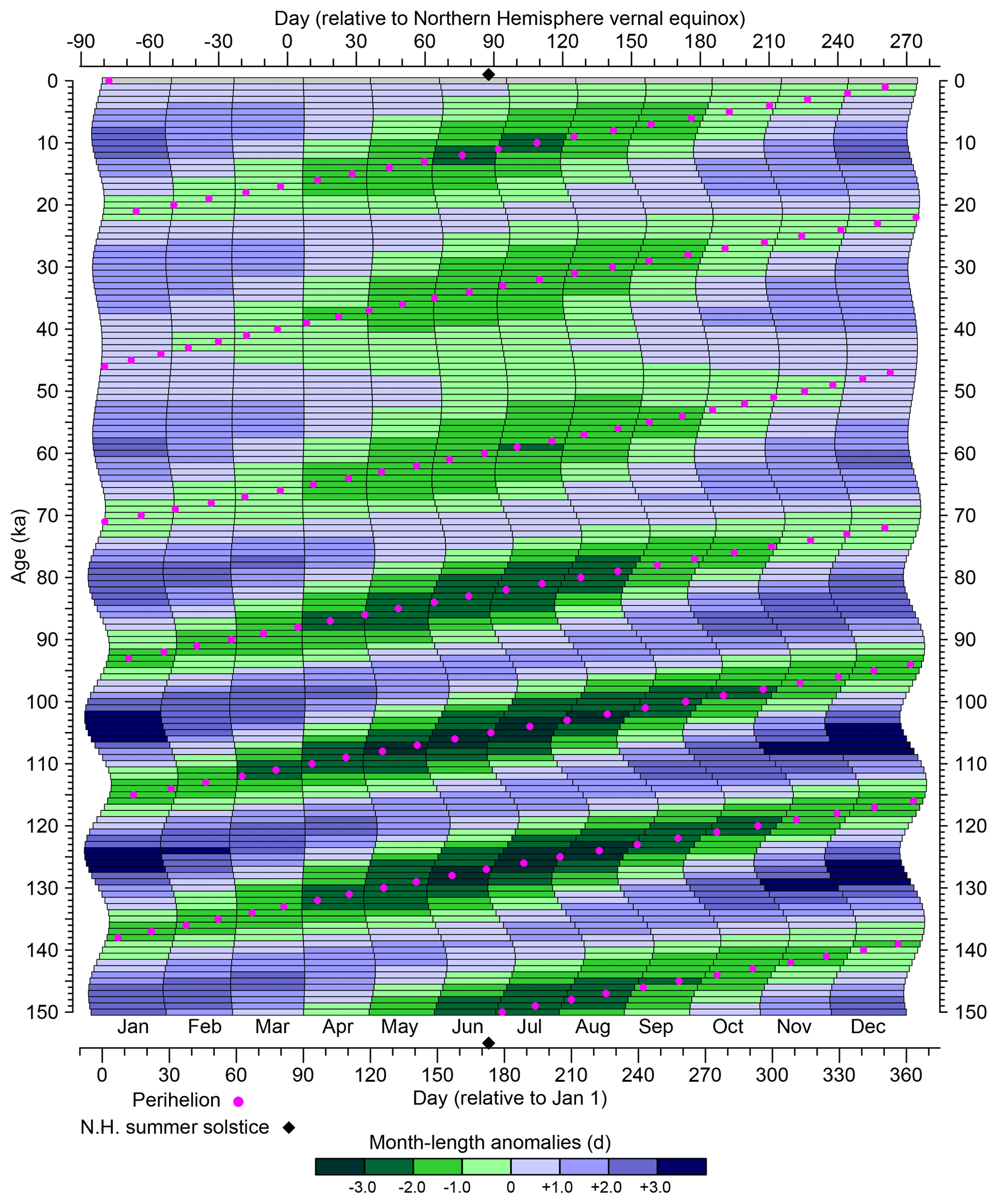
Figure 1Variations over the past 150 kyr in the beginning and ending days of fixed-angular months for a 365 d noleap calendar, shown for 1 kyr intervals beginning at 0 ka (1950 CE). The left side of each horizontal bar shows the beginning day, while the right side shows the ending day of a particular month for each 1 kyr interval. The month-length “anomalies” or differences from the present day are shown by shading, with individual paleo months that are shorter than those at present indicated by green shades and those that are longer indicated by blue shades. The day that perihelion occurs for each 1 kyr interval is indicated by a magenta dot, and the overall pattern of month-length anomalies can be seen to follow the day of perihelion. The figure shows that the changing month lengths move the beginning, middle, and ending days of each month (as well as the beginning and ending days of the year). The day of the Northern Hemisphere summer solstice is indicated by a black diamond on the x axes.
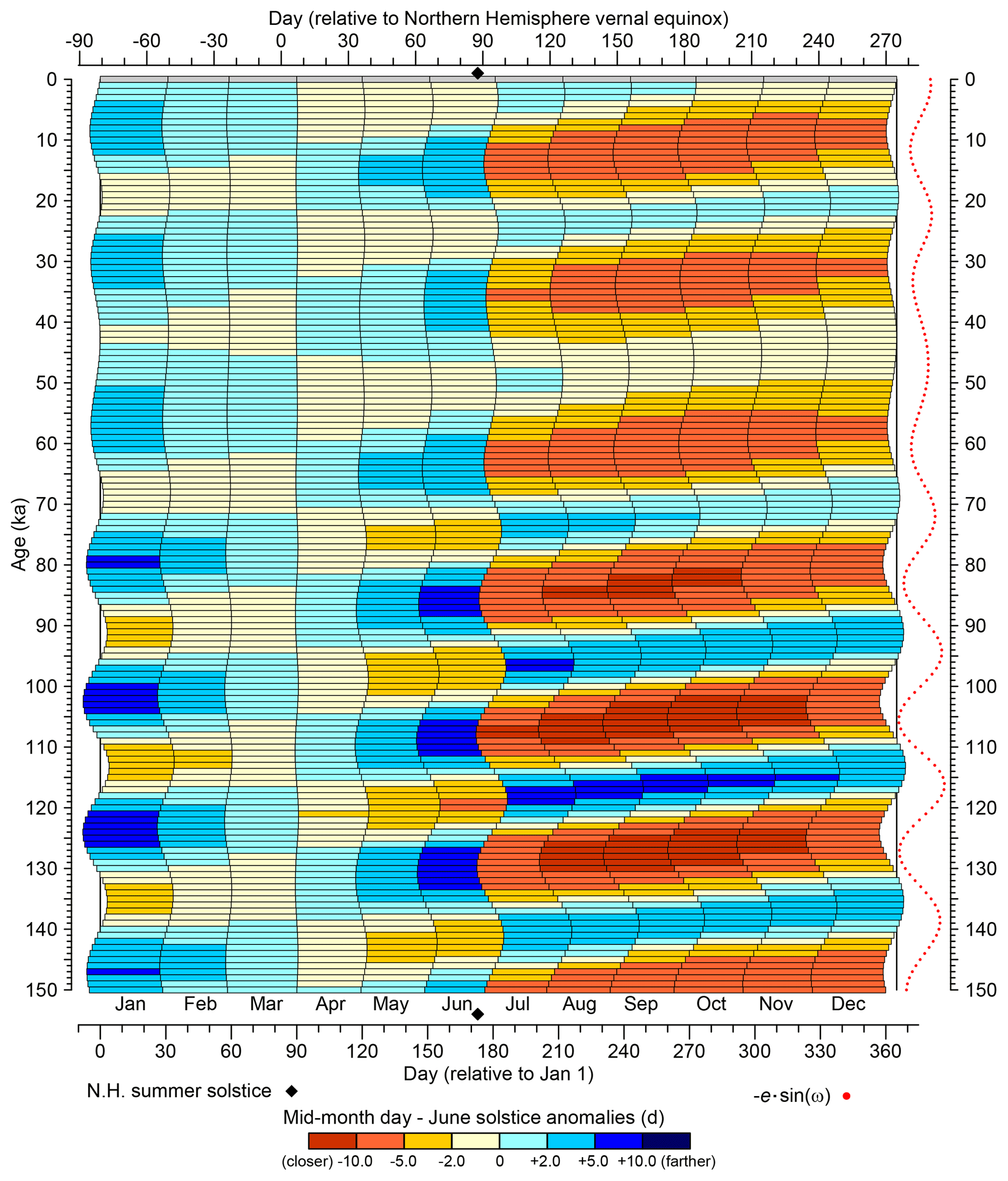
Figure 2Variations in the difference (in days) between the mid-month day of each month and the day of the June solstice. Months that are shifted closer to the June solstice are indicated by orange hues, while those that are farther away are indicated by blue. As in Fig. 1, variations over the past 150 kyr in the beginning and ending days of fixed-angular months for a 365 d noleap calendar are shown for 1 kyr intervals beginning at 0 ka (1950 CE). The left side of each horizontal bar shows the beginning day, while the right side shows the ending day of a particular month for each 1 kyr interval. Variations in the beginning and ending days of individual months can be seen to track the climatic precession parameter (e⋅sin ω, where e is eccentricity and ω is the longitude of perihelion measured from the vernal equinox, an index of Earth's distance from the Sun at the summer solstice), which is plotted at the right side of the figure (red dots). (Note that the inverse of the climatic precession parameter is plotted for easier comparison.) The day of the Northern Hemisphere summer solstice is indicated by a black diamond on the x axes.
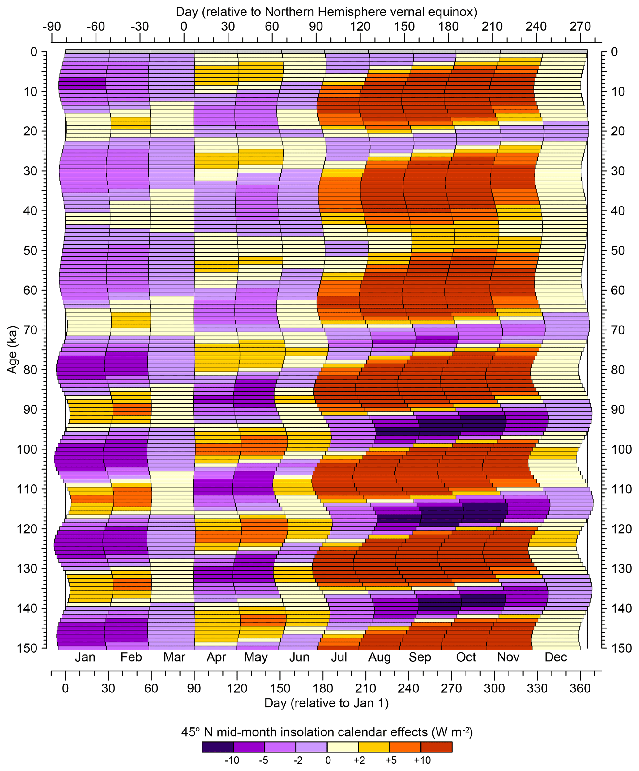
Figure 3Calendar effects on insolation at 45∘ N. The differences plotted show the values of average daily insolation at mid-month days identified using the appropriate fixed-angular paleo calendar minus those using the fixed-length definition of present-day months, with orange hues showing positive differences and purple hues negative differences. As in Fig. 1, variations over the past 150 kyr in the beginning and ending days of fixed-angular months for a 365 d noleap calendar are shown for 1 kyr intervals beginning at 0 ka (1950 CE). The left side of each horizontal bar shows the beginning day, while the right side shows the ending day of a particular month for each 1 kyr interval.
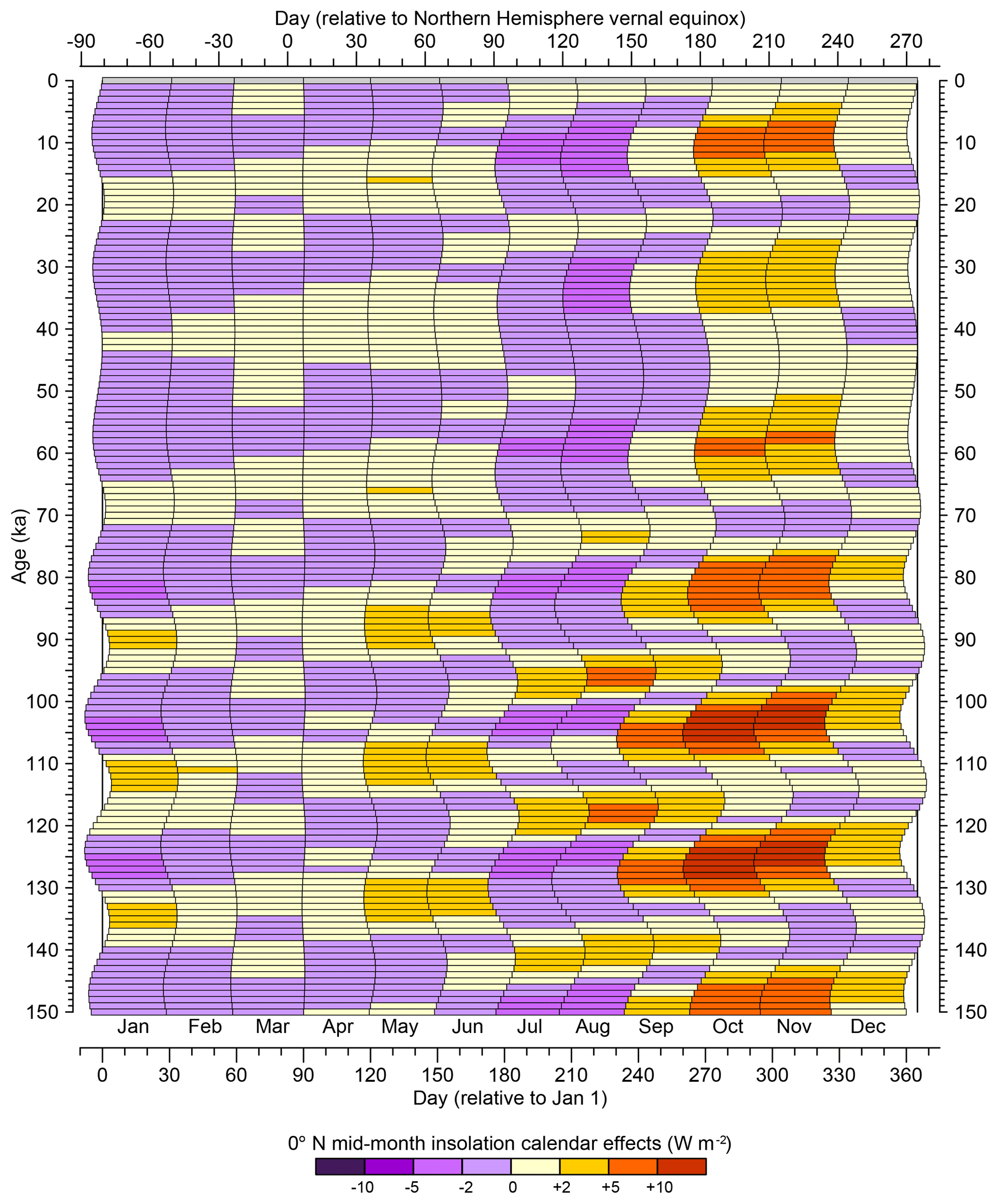
Figure 4Calendar effects on insolation at the Equator. The differences plotted show the values of average daily insolation at mid-month days identified using the appropriate fixed-angular paleo calendar minus those using the fixed-length definition of present-day months, with orange hues showing positive differences and purple hues negative differences. As in Fig. 1, variations over the past 150 kyr in the beginning and ending days of fixed-angular months for a 365 d noleap calendar are shown for 1 kyr intervals beginning at 0 ka (1950 CE). The left side of each horizontal bar shows the beginning day, while the right side shows the ending day of a particular month for each 1 kyr interval.

Figure 5Calendar effects on insolation at 45∘ S. The differences plotted show the values of average daily insolation at mid-month days identified using the appropriate fixed-angular paleo calendar minus those using the fixed-length definition of present-day months, with orange hues showing positive differences and purple hues negative differences. As in Fig. 1, variations over the past 150 kyr in the beginning and ending days of fixed-angular months for a 365 d noleap calendar are shown for 1 kyr intervals beginning at 0 ka (1950 CE). The left side of each horizontal bar shows the beginning day, while the right side shows the ending day of a particular month for each 1 kyr interval.
The beginnings and ends of each fixed-angular month in a 365 d noleap calendar are shown at 1 kyr intervals for the past 150 kyr in Fig. 1, calculated using the approach described in Sect. 4.2–4.5 below. (See Sect. 4.4.1 of the NetCDF Climate and Forecast Metadata Conventions (http://cfconventions.org, last access: 11 August 2019) for a discussion of climate-model output calendar types.) The month-length anomalies (i.e., long-term differences between paleo and present month lengths, with present defined as 1950 CE) are shown in color, with (paleo) months that are shorter than those at present in green shades and months that are longer than those at present in blue shades. Not only do the lengths of fixed-angular months vary over time, but so do their middle, beginning, and ending days (Fig. 2), with mid-month days that are closer to the June solstice indicated in orange and those that are farther from the June solstice in blue. The variations in month length (Fig. 1) obviously track the changing time of year of perihelion, while the beginning and ending day anomalies reflect the climatic precession parameter (Fig. 2). The shift in the beginning, middle, or end of individual months relative to the solstices ultimately controls the average or mid-month daily insolation at different latitudes (Figs. 3–5).
Figure 2 essentially maps the systematic displacement of the stack of horizontal bars for individual months, which reflects the changes during the year of the beginning and end of each month. Using 15 ka as an example, perihelion occurs on day 111.87 (relative to 1 January), and consequently the months between March and August are shorter than present (Fig. 1). That effect in turn moves the beginning, middle, and ending day of the months between April and December earlier in the year (Fig. 2). July therefore begins a little over 5 d earlier than at present, i.e., closer within the year to the June solstice. June is likewise displaced earlier in the year, with the beginning of the month 3.41 d farther from the June solstice and the end a similar number of days closer to the June solstice than at present. Thus, the calendar effect arises more from shifts in the timing (beginning, middle, and end) of the months than from changes in their lengths.
The calendar effect is illustrated below for four times: 6 and 127 ka are the target times for the planned warm-interval midHolocene and lig127k CMIP6–PMIP4 (Coupled Model Intercomparison Project Phase 6–Paleoclimate Modelling Intercomparison Project Phase 4) simulations (Otto-Bliesner et al., 2017) and illustrate the calendar effects when perihelion occurs in the boreal summer or autumn (Fig. 6); 116 ka is the time of a proposed sensitivity experiment for the onset of glaciation (Otto-Bliesner et al., 2017) and illustrates the calendar effect when perihelion occurs in boreal winter; and 97 ka was chosen to illustrate an orbital configuration not represented by the other times (i.e., one with boreal spring months occurring closer to the June solstice).
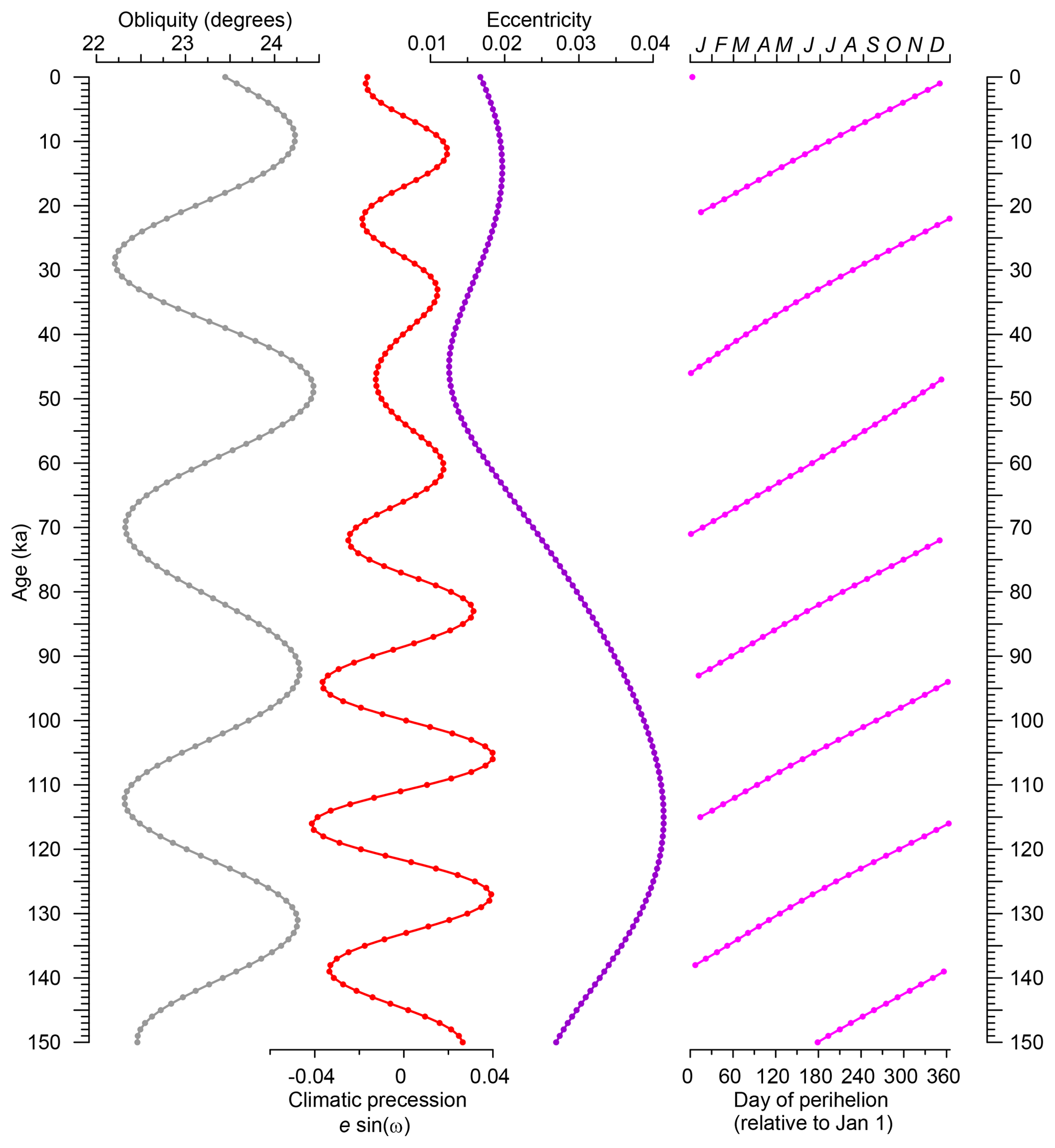
Figure 6Orbital parameter variations at 1 kyr intervals over the past 150 kyr for obliquity, climatic precession, eccentricity, and day of perihelion (relative to 1 January). Climatic precession is calculated as e⋅sin ω, where e is eccentricity and ω is the longitude of perihelion measured from the vernal equinox.
At 6 ka, perihelion occurred in September (Fig. 6), and the months from May through October were shorter than today (Fig. 1), with the greatest differences in August (1.65 d shorter than present). This contraction of month lengths moved the middle of all of the months from April through December closer to the June solstice (Fig. 2), with the greatest difference in November (5.01 d closer to the June solstice and therefore 5.01 d farther from the December solstice). At 127 ka, perihelion was in late June, and the months April through September were shorter than today (Fig. 1), with the greatest difference in July (3.19 d shorter than present). As at 6 ka, the shorter boreal summer months at 127 ka move the middle of the months between July and December closer to the June solstice (Fig. 2), with the greatest difference in September and October (12.80 and 12.70 d closer, respectively). At both 6 and 127 ka, the longer boreal winter months begin and end earlier in the year, placing the middle of January 3.38 (6 ka) and 4.35 (127 ka) days farther from the June solstice than at present. As can be noted in Figs. 1 and 2, 127 ka does not represent a simple amplification of 6 ka conditions. Although broadly similar in having shorter late boreal summer and autumn months that begin earlier in the year (and hence closer to the June solstice), the two times are only similar in the relative differences from the present in month length and beginning and ending days.
At 116 ka, perihelion was in late December, and consequently the months from October through March were shorter than present (Fig. 1). This has the main effect of moving the middle of the months July through December farther from the June solstice (with a maximum in September of 5.80 d; Fig. 2), somewhat opposite to the pattern at 6 and 127 ka. At 97 ka, perihelion occurred in mid-November, between its occurrence in September at 6 ka and December at 116 ka (Fig. 1). The impact on month length and mid-month timing is complicated, with the mid-month days of January through March and July through October occurring farther from the June solstice (Fig. 2).
The first-order impact of the calendar effect can be gauged by comparing (at a particular latitude) daily insolation values for mid-month days determined using the appropriate paleo calendar (which assumes fixed-angular definitions of months) with insolation values for mid-month days using the present-day calendar (which assumes fixed-length definitions of months). Using the example of 45∘ N, at 6 ka the shorter (than present) and earlier (relative to the June solstice) months of September through November had insolation values over 10 W m−2 (12.67, 15.59, and 10.38 W m−2, respectively) greater for mid-month days defined using the fixed-angular paleo calendar in comparison with values determined using the fixed-length present-day calendar (Fig. 3), and at 127 ka, the differences exceeded 35 W m−2 for the months of August through October (41.27, 49.74, and 38.66 W m−2, respectively). These positive insolation differences were accompanied by negative differences from January through June. At first glance, it may seem counterintuitive that the calendar effects that yield positive differences in mid-month insolation are not balanced by negative insolation differences, as is the case with the month-length differences. However, the calendar effects on insolation include both the month-length differences and long-term insolation differences themselves (Figs. 7–9), which are not symmetrical within the year, so the calendar effects do not “cancel out” within the year.

Figure 7Long-term differences in mid-month average daily insolation relative to present (0 ka or 1950 CE) at 45∘ N for a fixed-angular calendar. As in Fig. 1, variations over the past 150 kyr in the beginning and ending days of fixed-angular months for a 365 d noleap calendar are shown for 1 kyr intervals beginning at 0 ka (1950 CE). The left side of each horizontal bar shows the beginning day, while the right side shows the ending day of a particular month for each 1 kyr interval.

Figure 8Long-term differences in mid-month average daily insolation relative to present (0 ka or 1950 CE) at the Equator for a fixed-angular calendar. As in Fig. 1, variations over the past 150 kyr in the beginning and ending days of fixed-angular months for a 365 d noleap calendar are shown for 1 kyr intervals beginning at 0 ka (1950 CE). The left side of each horizontal bar shows the beginning day, while the right side shows the ending day of a particular month for each 1 kyr interval.
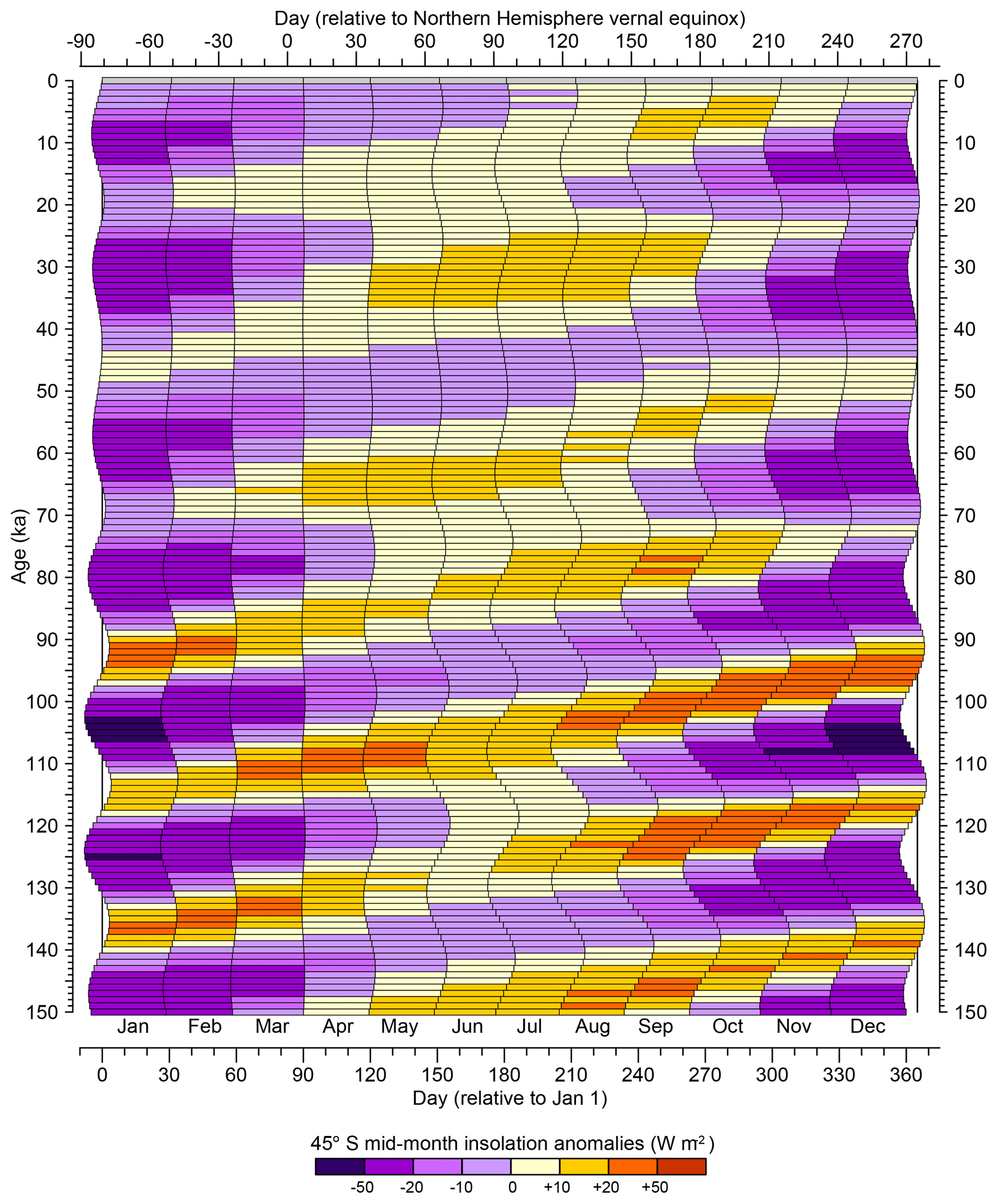
Figure 9Long-term differences in mid-month average daily insolation relative to present (0 ka or 1950 CE) at 45∘ S for a fixed-angular calendar. As in Fig. 1, variations over the past 150 kyr in the beginning and ending days of fixed-angular months for a 365 d noleap calendar are shown for 1 kyr intervals beginning at 0 ka (1950 CE). The left side of each horizontal bar shows the beginning day, while the right side shows the ending day of a particular month for each 1 kyr interval.
At 116 ka, the later occurring months of September and October had negative differences in mid-month insolation that exceeded 10 W m−2 (−14.80 and −15.23 W m−2, respectively; Fig. 3). For regions where surface temperatures are strongly tied to insolation with little lag, such as the interiors of the northern continents, these calendar effects on insolation will be directly reflected by the calendar effects on temperatures. By moving the beginning, middle, and end of individual months (and seasons) closer to or farther from the solstices, the “apparent temperature” of those intervals will be affected (i.e., months or seasons that start or end closer to the summer solstice will be warmer). The calendar effect on insolation varies strongly with latitude, with the sign of the difference broadly reversing in the Southern Hemisphere (Figs. 3–5).
Figures 3 to 5 show the calendar effect on insolation at three different latitudes (which are longitudinally uniform, and hence not much would be gained from mapping them), and that effect can be thought of as being compounded by the month-length effects superimposed on the time-varying insolation. The amplitude of the calendar effect on insolation in December at 45∘ N (Fig. 3) only occasionally exceeds the range between −2.0 and +2.0 W m−2 because it is winter in the Northern Hemisphere and insolation in general is low. Likewise, the calendar effects on insolation at 45∘ S (Fig. 5) are quite muted in June, which is winter in the Southern Hemisphere.
Past demonstrations of the calendar effect have used “real” paleoclimatic simulations, so the climate patterns being used in these demonstrations include both the calendar effect and the long-term mean differences in climate between the experiment and control simulations. Comparison of Figs. 3 and 7 clearly shows, however, that the variations over time in insolation and in the calendar effect are not identical, so the use of an actual paleoclimatic experiment (e.g., for 6 or 127 ka) to illustrate the calendar effect will inevitably be confounded by the climatic response to changes in insolation (and other boundary conditions). The impact on the analysis of paleoclimatic simulations of the calendar effect can alternatively be assessed by assuming that the long-term mean difference in climate (also referred to as the experiment minus the control “anomaly”) is zero everywhere, illustrating the “pure” calendar effect. Pseudo-daily interpolated values (or actual daily output, if available) of present-day monthly data can then simply be reaggregated using an appropriate paleo calendar and compared with the present-day data. (The pseudo-daily values used here were obtained by interpolating monthly data to a daily time step using the monthly-mean-preserving algorithm described below.)
The pure calendar effect is demonstrated here using present-day monthly long-term mean (1981–2010) values of near-surface air temperature (tas) from the Climate Forecast System Reanalysis (CFSR; Saha et al., 2010; https://esgf.nccs.nasa.gov/projects/ana4mips/, last access: 11 August 2019) and monthly precipitation rate (precip) from the CPC Merged Analysis of Precipitation (CMAP; Xie and Arkin, 1997; https://www.esrl.noaa.gov/psd/data/gridded/data.cmap.html, last access: 11 August 2019) (Fig. 10). These data were chosen because they are global in extent and are of reasonably high spatial resolution. The long-term mean values of both data sets follow an implied 365 d noleap calendar.
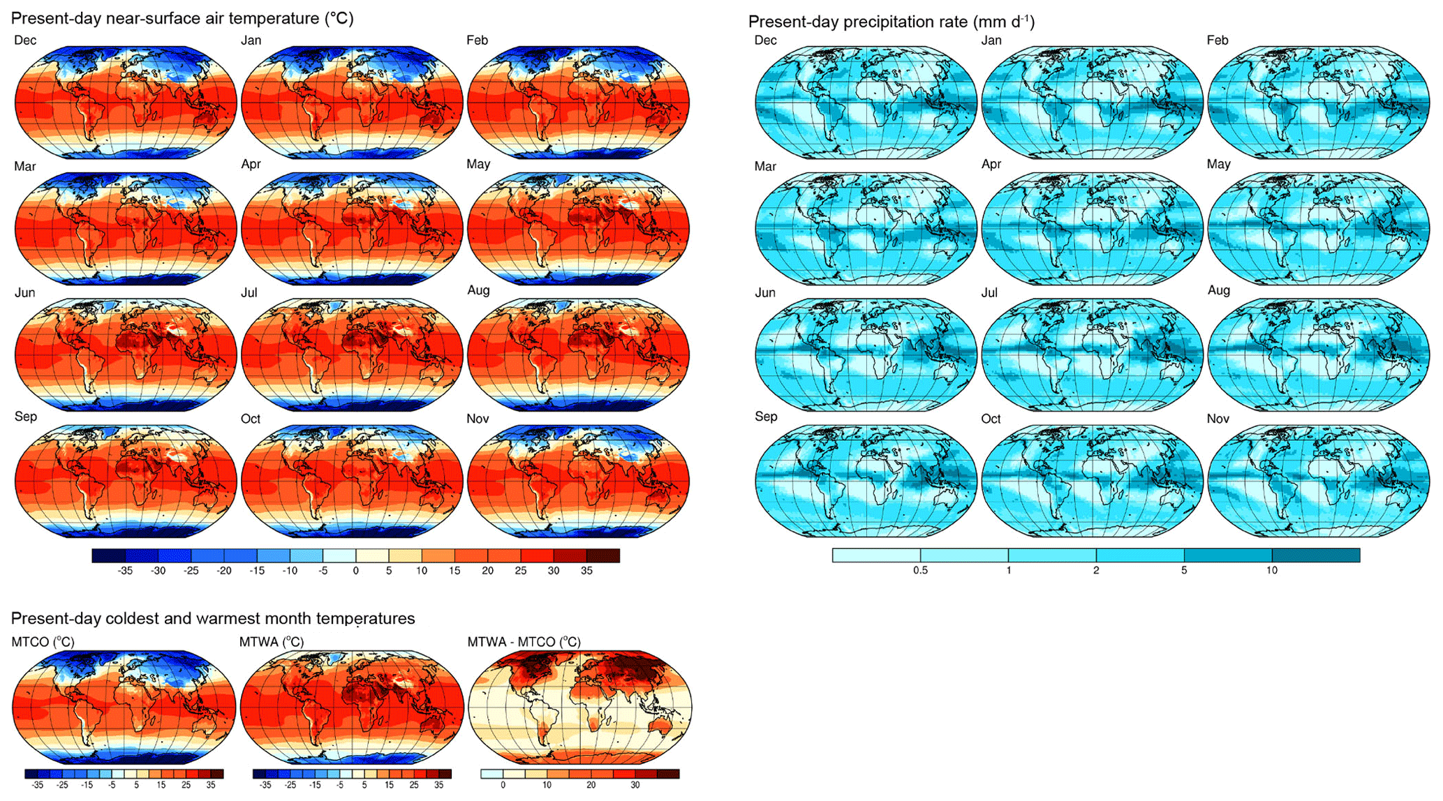
Figure 10Present-day (1981–2010 CE) long-term mean values of monthly near-surface air temperature (tas) from the Climate Forecast System Reanalysis (CFSR), the mean temperatures of the warmest (MTWA) and coldest (MTCO) months and their differences from the same data, and precipitation rate (precip) from the CPC Merged Analysis of Precipitation (CMAP).
If it is assumed that there is no long-term mean difference between a present-day and paleo simulation (by adopting the present-day data as the simulated paleo data), then the unadjusted present-day data can be compared with present-day data adjusted to the appropriate paleo month lengths. The calendar-adjusted minus unadjusted differences will therefore reveal the inverse of the built-in calendar-effect “signal” in the unadjusted data, which might readily be interpreted in terms of some specific paleoclimatic mechanisms while instead being a data analytical artifact. Positive values on the maps (Figs. 11–13) indicate, for example, where temperatures would be higher or precipitation greater if a fixed-angular calendar were used to summarize the paleo data.
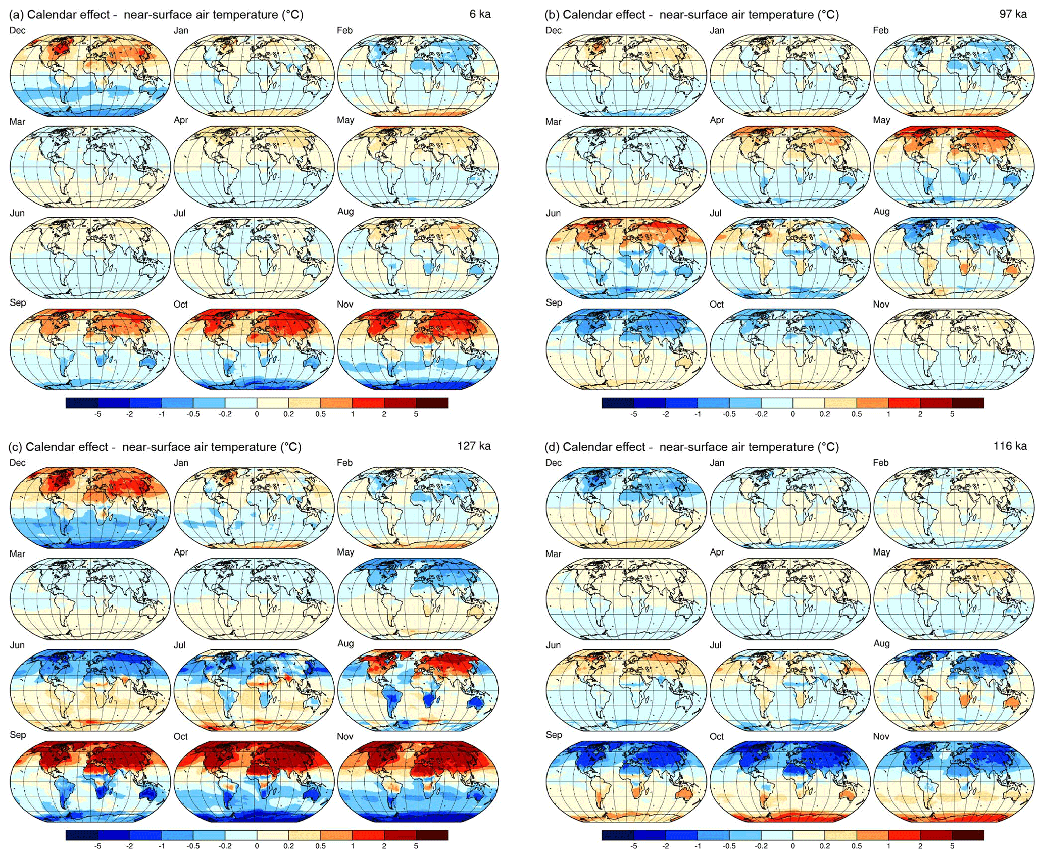
Figure 11Calendar effects on near-surface air temperature for 6 ka (a), 97 ka (b), 127 ka (c), and 116 ka (d). The maps show the patterns of month-length adjusted average temperatures minus the unadjusted values using 1981–2010 long-term averages of CFSR tas values, with positive differences (indicating that the adjusted data would be warmer than unadjusted data) in red hues and negative differences in blue.
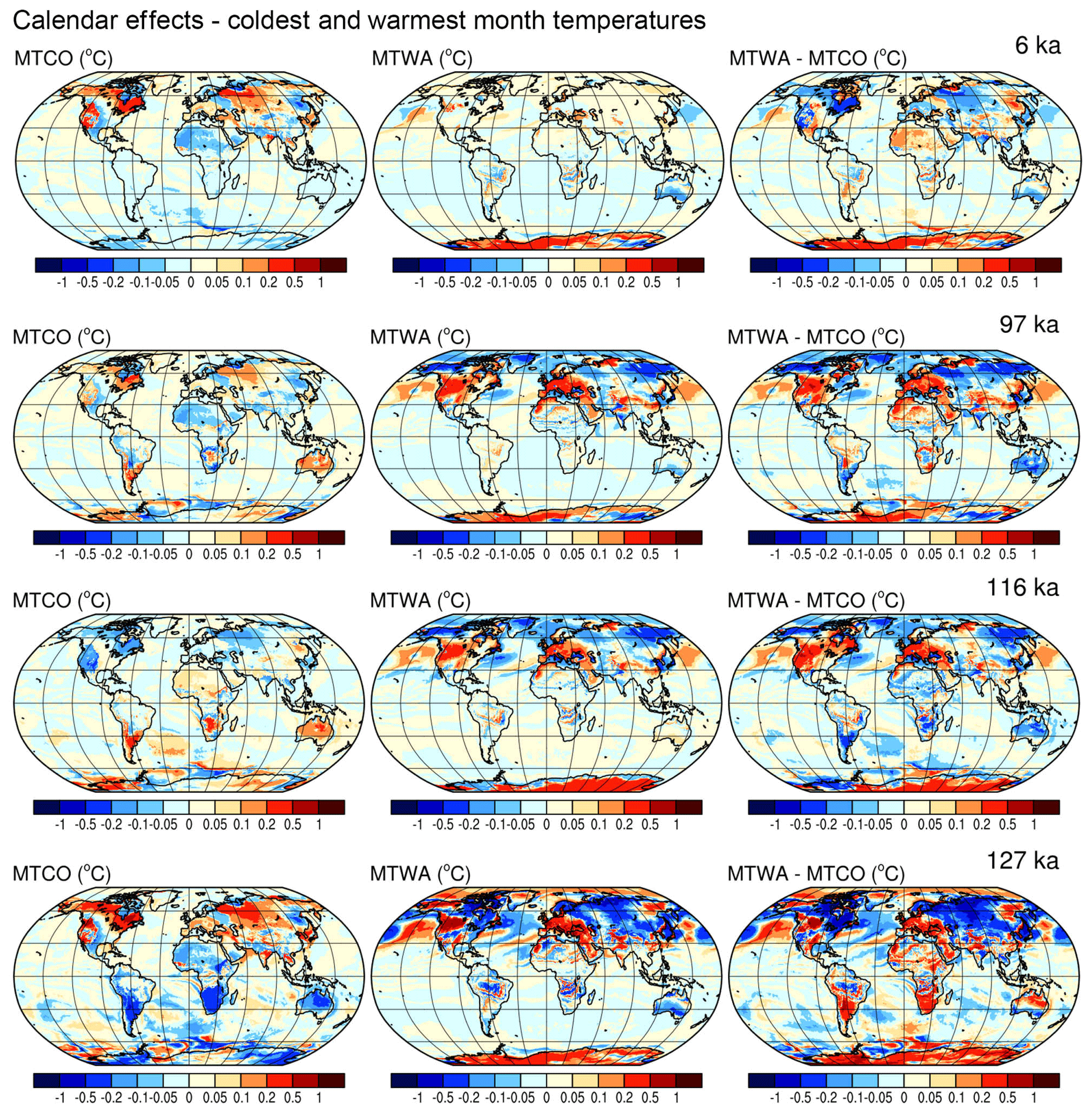
Figure 12Calendar effects on the mean near-surface air temperatures of the warmest (MTWA) and coldest (MTCO) months and their differences (an index of seasonality) for 6, 97, 116, and 127 ka (top to bottom row). The maps show the patterns of month-length adjusted average temperatures minus the unadjusted values for MTWA and MTCO using 1981–2010 long-term averages of CFSR tas values, with positive differences (indicating that the adjusted data would be warmer than unadjusted data) in red hues and negative differences in blue.
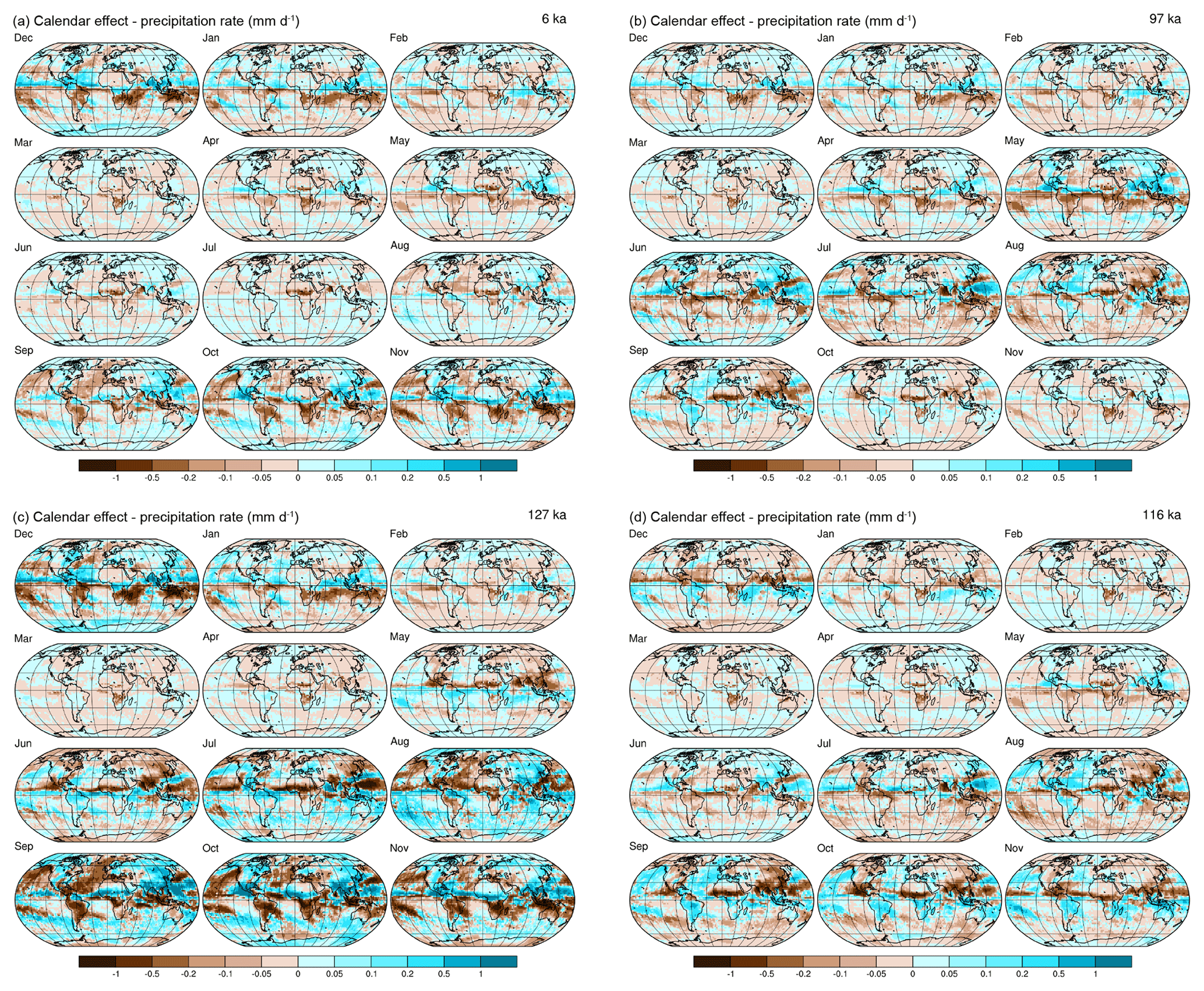
Figure 13Calendar effects on precipitation rate for 6 ka (a), 97 ka (b), 127 ka (c), and 116 ka (d). The maps show the patterns of month-length adjusted precipitation rate minus the unadjusted values using 1981–2010 long-term averages of CMAP precip values, with positive differences (indicating that the adjusted data would be wetter than unadjusted data) in blue hues and negative differences in brown.
3.1 Monthly temperature
The impacts of using the appropriate calendar to summarize the data (as opposed to not) are large, often exceeding 1 ∘C in absolute value (Fig. 11). The effects are spatially variable and are not simple functions of latitude, as might initially be expected, because the effect increases with the amplitude of the annual cycle (which has a substantial longitudinal component) for temperature regimes that are in phase with the annual cycle of insolation. For temperature regimes that are out of phase with insolation, the calendar-adjusted minus unadjusted values would be negative and largest when the temperature variations were exactly out of phase. (If there were no annual cycle, i.e., if a climate variable remained constant over the course of a year, the calendar effect would be zero.) The interaction between the annual cycle and the direct calendar effect on insolation produces patterns of the overall calendar effect that happen to resemble some of the large-scale responses that are frequently found in climate simulations, both past and future, such as high-latitude amplification or damping, continent–ocean contrasts, interhemispheric contrasts, and changes in the seasonality of temperature (see Izumi et al., 2013). Because the month-length calculations use the Northern Hemisphere vernal equinox as a fixed origin for the location of Earth along its orbit, the effects seem to be small during the months surrounding the equinox (i.e., February through April; Fig. 11), and indeed the selection of a different origin would produce different apparent effects (see Joussaume and Braconnot, 1997; Sect. 2.1). However, the selection of a different origin would not change the relative (to present) length of time it would take Earth to transit any particular angular segment of its orbit.
At 6 ka, the largest calendar effects on temperature can be observed over the Northern Hemisphere continents for the months from September through December (Fig. 11), consistent with the earlier beginning of these months (Fig. 2) and the direct calendar effect on insolation at 45∘ N (Fig. 3). For example, in the interior of the northern continents, as well as North Africa, temperature is in phase with insolation, and therefore the calendar effect on insolation (Fig. 3), which produces strongly positive differences from August through November, is reflected by the calendar effect on temperature. Over the northern oceans, temperature is broadly in phase with insolation but with a lag, which reduces the magnitude of the effect and gives rise to an apparent land–ocean contrast that otherwise might be interpreted in terms of some particular paleoclimatic mechanism. The calendar effect on temperature from January through March produces negative calendar-adjusted minus unadjusted values in the northern continental interiors (Fig. 11), which is also consistent with the calendar effect on insolation. In the Southern Hemisphere at 6 ka, the calendar effects on temperature produce generally negative differences, which is consistent with the calendar effects on mid-month insolation at 45∘ S (Fig. 5) that produce generally negative differences throughout the year, particularly during the months of August through November. Like the continent–ocean contrast in the Northern Hemisphere, the Northern Hemisphere–Southern Hemisphere contrast in the calendar effect on temperature could also be interpreted in terms of one or another of the mechanisms thought to be responsible for interhemispheric temperature contrasts.
At 127 ka, the calendar effect on temperature is broadly similar to that at 6 ka over the months from September through March, but it differs in sign from April through July and in magnitude in August (Fig. 11). These patterns are also consistent with the direct calendar effects on insolation. At 127 ka, the calendar effect on insolation produces strongly positive differences in the Northern Hemisphere earlier in the northern summer than at 6 ka (Fig. 3), while at 45∘ S the calendar effect on insolation produces strongly negative differences in July and persists that way through November (Fig. 5). At 116 ka, perihelion occurs in late December in comparison to late June at 127 ka (Figs. 1 and 6), and not surprisingly the calendar effect on temperature is nearly the inverse of that at 127 ka (Fig. 11). This pattern has important implications for paleoclimatic studies because in addition to all of the changes in the forcing and the paleoclimatic responses accompanying the transition out of the last interglacial, the possibility that some of the apparent simulated changes between 127 and 116 ka may be an artifact of data analysis procedures cannot be discounted.
At 97 ka, a time selected to illustrate a different orbital configuration (i.e., one with boreal spring months occurring closer to the June solstice) than the similar (6 and 127 ka) or contrasting (127 and 116 ka) configurations, the calendar effect on temperature in the Northern Hemisphere (Fig. 11) shows a switch from positive differences in the early boreal summer (May and June) to negative in the late summer (August and September). This switch is again consistent with the direct calendar effect on insolation (Fig. 3). Like the other times, these spatial variations in the calendar effect could easily be interpreted in terms of one kind of paleoclimatic mechanism or another.
The generally larger calendar effect on temperature over the continents than over the oceans implicates the amplitude of the seasonal cycle in the size of the effect. This situation suggests that even in model-only intercomparisons (and even in the unlikely case that all models involved in an intercomparison use the same calendar) the calendar effect could be present because the amplitude of the seasonal cycle is dependent on model spatial resolution (and its influence on model orography).
3.2 Mean temperature of the warmest and coldest months
Although the calendar effects on monthly mean temperature show some subcontinental-scale variability, the overall patterns are of relatively large spatial scales and are interpretable in terms of the direct orbital effects on month lengths and insolation. The calendar effects on the mean temperature of the warmest (MTWA) and coldest (MTCO) calendar months (and their differences) are much more spatially variable (Fig. 12). This variability arises in large part because of the way these variables are usually defined (e.g., as the mean temperature of the warmest or coldest conventionally defined month as opposed to the temperature of the warmest or coldest 30 d interval), but also because the calendar adjustment can result in a change in the specific month that is warmest or coldest. These effects are compounded when calculating seasonality (as MTWA minus MTCO). Other definitions of the warmest and coldest month are possible, such as the warmest consecutive 30 d period during the year (e.g., Caley et al., 2014), and such definitions will not be susceptible to the calendar effect. In practice, however, paleoclimatic reconstructions based on calibrations or forward-model simulations routinely use conventional calendar-month definitions of the warmest and coldest months and of seasonality (Bartlein et al., 2011; Harrison et al., 2014), and often only monthly output from paleoclimatic simulations is available, necessitating consistent definitions when summarizing model output.
In the particular set of example times chosen here, the magnitudes of the calendar effects are also smaller than those of individual months because, as it happens, the calendar effects in January and February (typically the coldest months in the Northern Hemisphere) and July and August (typically the warmest months in the Northern Hemisphere) are not large. There are also some surprising patterns. The inverse relationship between the calendar effects at 116 and 127 ka that might be expected from inspection of the monthly effects (Fig. 11) are not present, while the calendar effects on MTCO and MTWA at 97 and 116 ka tend to resemble one another (Fig. 12). Across the four example times, there is an indistinct but still noticeable pattern in reduced seasonality (MTWA minus MTCO) between the adjusted and unadjusted values, which like the other patterns described above could tempt interpretation in terms of some specific climatic mechanisms.
3.3 Monthly precipitation
In contrast to the large spatial-scale patterns of the calendar effect on temperature, the patterns of the calendar effect on precipitation rate are much more complex, showing both continental-scale patterns (like those for temperature) and smaller-scale patterns that are apparently related to precipitation associated with the ITCZ and regional and global monsoons (Fig. 13). The continental-scale patterns are evident in the calendar effects at 6 and 127 ka, particularly in the months from September through November (Fig. 13), when it can also be noted (especially over the midlatitude continents in both hemispheres) that there is a positive association with the calendar effect on temperature. This association is simply related to similarities in the shapes of the annual cycles of those variables and not to some kind of more elaborate thermodynamic constraint. At 116 ka, as for temperature, the large-scale calendar-effect patterns appear to be nearly the inverse of those at 127 ka. The smaller-scale kind of pattern is well illustrated at 127 ka in the tropical North Atlantic, sub-Saharan Africa, and south Asia. There, negative calendar-adjusted minus unadjusted values can be noted for June through August, giving way to positive differences from September through November, and the same transition appears inversely at 116 ka. Another example can be found in the South Pacific Convergence Zone in austral spring and early summer (September through November) at 6 and 127 ka, when generally positive differences between calendar-adjusted and unadjusted values in July and August give way to negative differences from September through December. This second kind of pattern, most evident in the subtropics, is not mirrored by the calendar effects on temperature.
Overall, the magnitude and spatial patterns of the calendar effects on temperature and precipitation (Figs. 11 and 13) resemble those in the paleoclimatic simulations and observations that we attempt to explain in mechanistic terms (Harrison et al., 2016). Depending on the sign of the effect, neglecting to account for the calendar effects could spuriously amplify some signals in long-term mean differences between the experiment and control simulations, while damping others.
3.4 Calendar effects and transient experiments
Calendar effects must also be considered in the analysis of transient climate-model simulations (even if those data are available on the daily time step). This can be illustrated for a variety of variables and regions using data from the TraCE-21ka transient simulations (Liu et al., 2009; https://www.earthsystemgrid.org/project/trace.html, last access: 11 August 2019). The series plotted in Fig. 14 are area averages for individual months on a yearly time step, with 100-year (window half-width) locally weighted regression curves added to emphasize century-timescale variations. The original yearly time-step data were aggregated using a perpetual noleap (365 d) calendar (using the present-day month lengths for all years). The gray and black curves in Fig. 14 show these unadjusted “original” values, while the colored curves show month-length adjusted values (i.e., pseudo-daily interpolated values, reaggregated using the appropriate paleo fixed-angular calendar). Area averages were calculated for ice-free land points.
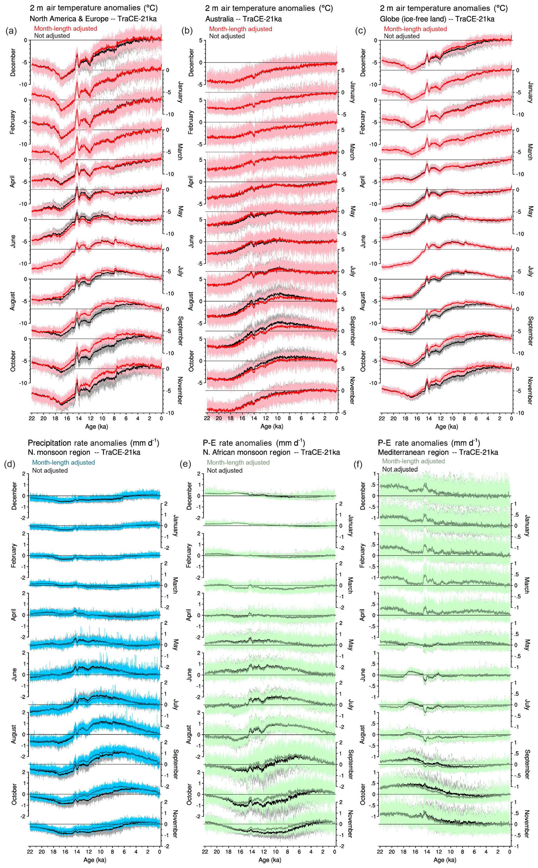
Figure 14Time series of original and month-length adjusted annual area-weighted averages of TraCE-21ka data (Liu et al., 2009), expressed as differences from the 1961–1989 long-term mean for (a–c) 2 m air temperature, (d) precipitation rate, and (e–f) precipitation minus evaporation (P−E). The original or unadjusted data are plotted in gray and black, and the adjusted data are in color. The area averages are grid-cell area-weighted values for land grid points in each region, and the smoother curves are locally weighted regression curves with a window half-width of 100 years. The regions are defined as (a) 15 to 75∘ N and −170 to 60∘ E, (b) 10 to 50∘ S and 110 to 160∘ E, (c) global ice-free land area, (d) 0 to 30∘ N and −30 to 120∘ E, (e) 5 to 17∘ N and −5 to 30∘ E, and (f) 31 to 43∘ N and −5 to 30∘ E.
Figure 14a shows area-weighted averages for 2 m air temperature for a region that spans 15 to 75∘ N and −170 to 60∘ E, the region used by Marsicek et al. (2018) to discuss Holocene temperature trends in simulations and reconstructions. The largest differences between month-length adjusted values and unadjusted values occur in October between 14 and 6 ka, when perihelion occurred during the northern summer months. October month lengths during this interval were generally within 1 d of those at present (Fig. 1), but the generally shorter months from April through September resulted in Octobers beginning up to 10 d earlier in the calendar than at present, i.e., closer in time to the boreal summer solstice (Fig. 2). The calendar-effect-adjusted October values therefore average up to 4 ∘C higher than the unadjusted values during this interval (Fig. 14a), consistent with the direct calendar effects on insolation at 45∘ N (Fig. 3). The calendar effect also changes the shape of the temporal trends in the data, particularly during the Holocene. October temperatures in the unadjusted data showed a generally increasing trend over the Holocene (i.e., since 11.7 ka), reaching a maximum around 3 ka, comparable with present-day values, while the adjusted data reached levels consistently above present-day values by 7.5 ka. The unadjusted October temperature data could be described as reaching a “Holocene thermal maximum” only in the late Holocene (i.e., after 4 ka), while the adjusted data display more of a mid-Holocene maximum. As is the case with the mapped assessments of the pure calendar effect, the differences between unadjusted and adjusted time series are of the kind that could be interpreted in terms of various hypothetical mechanisms. For example, the calendar-effect adjustment advances the time of the occurrence of a Holocene thermal maximum in October by about 3 kyr for North America and Europe.
As in North America and Europe, the adjusted temperature trends in Australia (10 to 50∘ S and 110 to 160∘ E) (Fig. 14b) are consistent with the direct calendar effects on insolation (i.e., for 45∘ S; Fig. 5). The difference between adjusted and unadjusted values are again largest in October between 14 and 6 ka, but the difference is the inverse of that for the North America and Europe region because the annual cycle of temperature for Australia is inversely related to the annual cycle of the insolation anomalies (Fig. 9) and therefore to the direct calendar effects on insolation (Fig. 5). Again, the shapes of the Holocene trends in the adjusted and unadjusted data are noticeably different. In the Australia (Fig. 14b) and North America and Europe (Fig. 14a) examples, relatively large areas are being averaged, and the calendar effect becomes more apparent as the size of the area decreases. Notably, the effect does not completely disappear at the largest scales, i.e., for area-weighted averages for the globe (for ice-free land grid cells) (Fig. 14c). The differences are smaller but still discernible.
In the Northern Hemisphere (African–Asian) monsoon region (0 to 30∘ N and −30 to 120∘ E), the calendar effects on precipitation rate are similar to those on temperature in the midlatitudes because the annual cycle of precipitation is roughly in phase with that of insolation (Fig. 7). There is little effect in the winter and spring but a substantial effect in summer and autumn over the interval from 17 to about 3 ka (Fig. 14d). The calendar effect reverses sign between July and August (when the month-length adjusted precipitation rate values are less than the unadjusted ones) and September and October (when the adjusted values are greater than the unadjusted ones). In July, the timing of relative maxima and minima in the two data sets is similar, while in October, in particular, the Holocene precipitation maximum is several thousand years earlier in the adjusted data than in the unadjusted data.
The time-series expression of the latitudinally reversing calendar effect on precipitation rate evident in Fig. 13 (e.g., July vs. October at 127 ka) can be illustrated by comparing precipitation or precipitation minus evaporation (P−E) for the North African (sub-Saharan) monsoon region (5 to 17∘ N and −5 to 30∘ E) with the Mediterranean region (31 to 43∘ N and −5 to 30∘ E) (Fig. 14e and f). The differences between the adjusted and unadjusted data in the North African region (Fig. 14e) parallel that of the larger monsoon region (Fig. 14d). The Mediterranean region, which is characteristically moister in winter and drier in summer, shows the reverse pattern: when the calendar-adjusted minus unadjusted P−E difference is positive in the monsoon region, it is negative in the Mediterranean region. Dipoles are frequently observed in climatic data, both present-day and paleo, and are usually interpreted in terms of broad-scale circulation changes in the atmosphere or ocean. This example illustrates that they could also be artifacts of the calendar effect. Such changes in the timing of extrema could also influence the interpretation of phase relationships among simulated time series and time series of potential forcing (Joussaume and Braconnot, 1997; Timm et al., 2008; Chen et al., 2011).
There are other interesting patterns in the monthly time series from the transient simulations, some of which are amplified by the calendar effect and others damped. The monthly time series suggest that the traditional meteorological seasons (i.e., December–February, March–May, June–August, September–November) are not necessarily the optimal way to aggregate data – the September time series in Fig. 14 often look like they are more similar to, and should be grouped with, July and August rather than with October and November, the traditional other (northern) autumnal months. Figure 14a (North America and Europe), for example, suggests that the July through November time series are similar in their overall trends, and even more so for the adjusted data (in pink and red). Similarly, months that appear highly correlated over some intervals (e.g., July and June global temperatures from the Last Glacial Maximum to the Holocene) become decoupled at other times. The impacts of the calendar effect on temporal trends in transient simulations (Fig. 14), when compounded by the spatial effects (Figs. 11–13), make it even more likely that spurious climatic mechanisms could be inferred in analyzing transient simulations rather than in the simpler time-slice simulations.
3.5 Summary
Several observations can be made about the calendar effect and its potential role in the interpretation of paleoclimatic simulations and comparisons with observations.
-
The variations in eccentricity and perihelion over time are large enough to produce differences in the length of (fixed-angular) months that are as large as 4 or 5 d, as well as differences in the beginning and ending times of months on the order of 10 d or more (Fig. 1).
-
These month-length and beginning and ending date differences are large enough to have noticeable impacts on the location in time of a fixed-length month relative to the solstices and hence on the insolation receipt during that interval (Figs. 2 through 5). The average insolation (and its difference from the present) during a fixed-length month will thus include the effects of the orbital variations on insolation and the changing month length.
-
However, such insolation effects are not offset by the changing insolation itself but instead can be reinforced or damped (Figs. 7 through 9). (In other words, orbitally related variations in insolation do not take care of the calendar definition issue.)
-
The pure calendar effects on temperature and precipitation (illustrated by comparing adjusted and non-adjusted data assuming no climate change; Figs. 11–13) are large, spatially variable, and could easily be mistaken for real paleoclimatic differences (from the present).
-
The impact of the calendar effect on transient simulations is also large (Fig. 14), affecting the timing and phasing of maxima and minima, which, when combined with the spatial impacts of the calendar effect, makes transient simulations even more prone to misinterpretation.
The approach we describe here for adjusting model output reported either as monthly data (using fixed-length definitions of months) or as daily data to reflect the calendar effect (i.e., to make month-length adjustments) has two fundamental steps: (1) pseudo-daily interpolation of the monthly data on a fixed-month-length calendar (which, when actual daily data are available, is not necessary), followed by (2) aggregation of those daily data to fixed-angular months defined for the particular time of the simulations. The second step obviously requires the calculation of the beginning and ending days of each month as they vary over (geological) time, which in turn depends on the orbital parameters. The definition of the beginning and ending days of a month in a leap-year, Gregorian, or proleptic Gregorian calendar (http://cfconventions.org) additionally depends on the timing of the (northern) vernal equinox, which varies from year to year. Here we describe the pseudo-daily interpolation method first, followed by a discussion of the month-length calculations. Then we describe the calendar-adjustment program, along with a few demonstration programs that exercise some of the individual procedures. All of the programs, written in Fortran 90, are available (see the “Code and data availability” section).
4.1 Pseudo-daily interpolation
The first step in adjusting monthly time-step model output to reflect the calendar effect is to interpolate the monthly data (either long-term means or time-series data) to pseudo-daily values (a step that is not required if the data are daily time-step values). It turns out that the most common way of producing pseudo-daily values, linear interpolation between monthly means, is not mean preserving; the monthly (or annual) means of the interpolated daily values will generally not match the original monthly values. An alternative approach, and the one we use here, is the mean-preserving “harmonic” interpolation method of Epstein (1991), which is easy to implement and performs the same function as the parabolic-spline interpolation method of Pollard and Reusch (2002). As is also the case with Pollard and Reusch's (2002) method, Epstein's (1991) approach can occasionally produce overshoots that are physically impossible, as can happen in the application of the method to variables like precipitation, which may have monthly values that alternate between zero and nonzero values. For practical reasons, variables like precipitation are therefore “clamped” at zero, which can introduce small differences between the annual and monthly means of the original and interpolated data, and we illustrate a pathological case of this below.
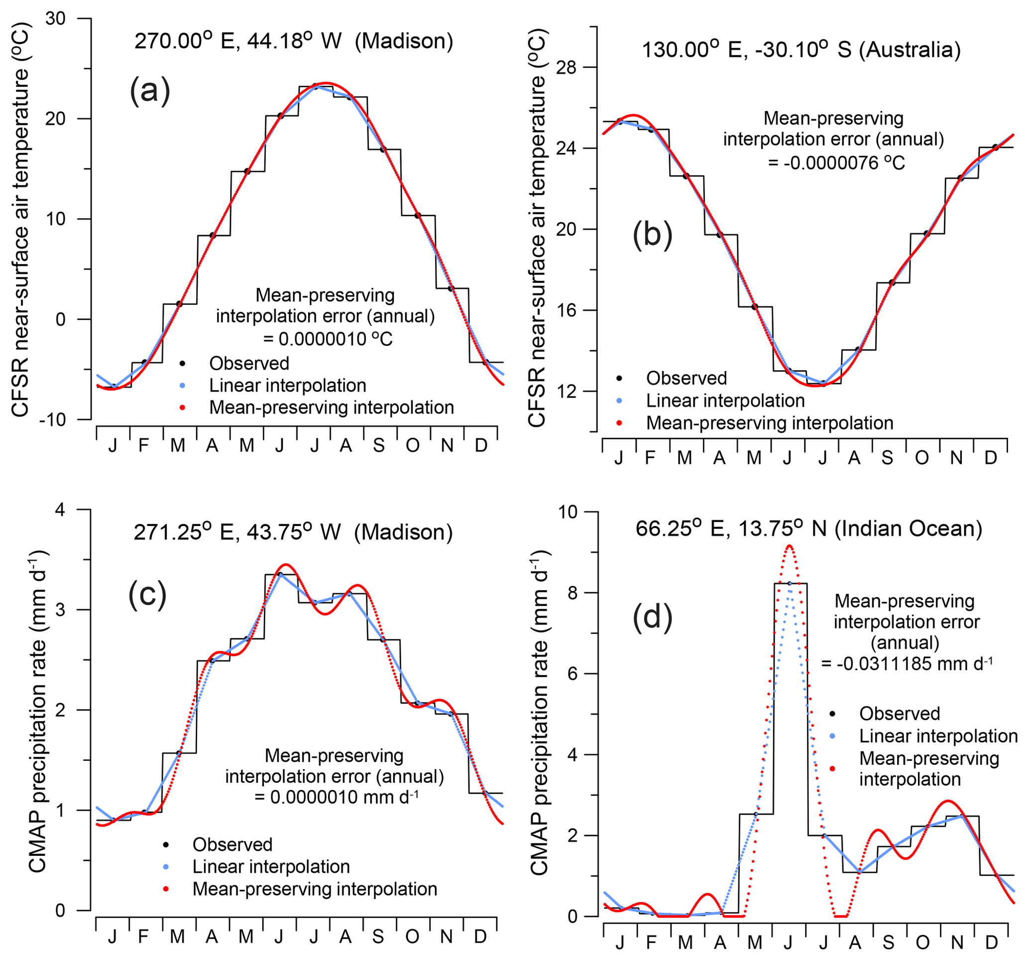
Figure 15Pseudo-daily interpolated temperature (a, b) and
precipitation (c, d) for some representative locations: (a, c) Madison, Wisconsin, USA, (b) Australia, and (d) the Indian Ocean. The
original monthly mean data are shown by the black dots and stepped curves
(black lines), daily values linearly interpolated between the monthly mean
values are shown in blue, and daily values using the mean-preserving
approach of Epstein (1991) are shown in red. The annual interpolation error
(or the difference between the annual average calculated using the original
data and the pseudo-daily interpolated data) is given for the
mean-preserving approach in each case. The interpolated data for this figure
were generated using the program demo_01_pseudo_daily_interp.f90.
The linear and mean-preserving interpolation methods can be compared using the Climate Forecast System Reanalysis (CFSR) near-surface air temperature and CPC Merged Analysis of Precipitation (CMAP) 1981–2010 long-term mean data (Fig. 15). A typical example for temperature appears in Fig. 15a for a grid point near Madison, Wisconsin (USA). The difference between the annual mean values of the interpolated data for the two approaches is small and similar (ca. ), but the difference between the original monthly means and the monthly mean of the linearly interpolated daily values can exceed 0.8 ∘C in some months (e.g., December). (The differences from the original monthly means for the mean-preserving interpolation method are less than ∘C for every month in Fig. 15a.) Figure 15b shows an example for a grid point in Australia, where again the difference between the original monthly means and the monthly means of the linearly interpolated daily values is not negligible (i.e., 0.4 ∘C). Similar results hold for precipitation (Fig. 15c), whereby the difference can exceed 0.1 mm d−1. Like other harmonic-based approaches, the Epstein (1991) approach can create interpolated curves that are wavy (see Pollard and Reusch, 2002, for a discussion), but these effects are small enough to not be practically important in nearly all cases. The pathological case for precipitation is shown in Fig. 15d at a grid point in the Indian Ocean. Here, the difference between an original monthly mean value and one calculated using the mean-preserving interpolation method reaches −0.12 mm d−1 in March and April, but the differences between the original monthly means and the monthly means of the linearly interpolated daily values are nearly 3 times larger.
The map patterns of the interpolation errors (the monthly mean values recalculated using the linear or mean-preserving pseudo-daily interpolated values minus the original values) appear in Fig. 16. (Note the differing scales for the linear interpolation errors and the mean-preserving interpolation errors.) The linear interpolation errors are quite large, with absolute values exceeding 1 ∘C and 1 mm d−1, and have distinct seasonal and spatial patterns: underpredictions of Northern Hemisphere temperature in summer (and overpredictions in winter), underpredictions of precipitation in the wet season (e.g., southern Asia in July), and overpredictions in the dry season (southern Asia in May). The magnitude and patterns of these effects again rival those we attempt to infer or interpret in the paleo record. The mean-preserving interpolation errors for temperature are very small and show only vague spatial patterns (note the differing scales). The errors for precipitation are also quite small but can be locally larger, as in the pathological case illustrated above. However, the map patterns of the interpolation errors strongly suggest that those cases are not practically important.
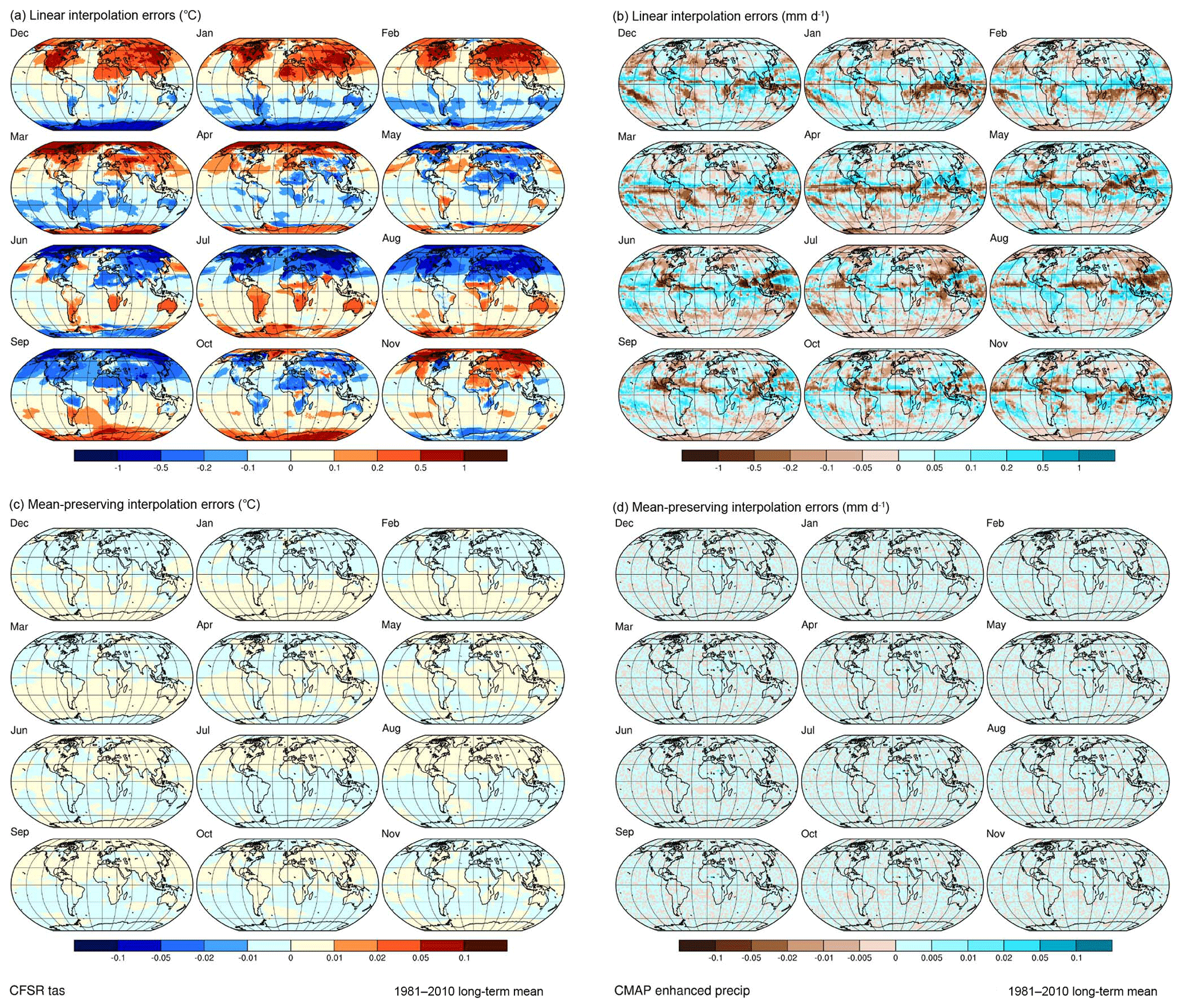
Figure 16Pseudo-daily interpolation errors for CFSR near-surface air temperature (a, c) and CMAP precipitation rate (b, d). (a, b) The interpolation errors, or the differences between the original monthly mean values and the monthly mean values recalculated from linear interpolation of pseudo-daily values. (c, d) The interpolation errors for mean-preserving (Epstein, 1991) interpolation. The errors for linear interpolation of the temperature data (∘C) range from −1.20851 to 1.29904, with a mean of 0.05664 and standard deviation of 0.16129 (over all months and grid points), while those for mean-preserving interpolation range from −0.00002 to 0.00050, with a mean of −0.0061 and standard deviation of 0.00007. The errors for linear interpolation of the precipitation data (mm d−1) range from −1.10617 to 1.40968, with a mean of 0.00087 and standard deviation of 0.11851, while those for mean-preserving interpolation range from −0.00002 to 0.00383, with a mean of 0.00001 and standard deviation of 0.00163.
The mean-preserving interpolation method is implemented in the Fortran 90
module named pseudo_daily_interp_subs.f90. The subroutine hdaily(…)
manages the interpolation, first getting the harmonic coefficients (Eq. 6 of
Epstein, 1991) using the subroutine named harmonic_coeffs(…) and then applying these coefficients in the
subroutine xdhat(…) to get the interpolated values.
4.2 Month-length calculations
The calculation of the length and the beginning, middle, and ending (real number or fractional) days of each month at a particular time is based on an approach for calculating orbital position as a function of time using Kepler's equation:
where M is the angular position along a circular orbit (referred to by astronomers as the mean anomaly), ε is eccentricity, and E is the eccentric anomaly (Curtis, 2014; Eq. 3.14). Given the angular position of the orbiting body (Earth) along the elliptical orbit, θ (the “true anomaly”), E can be found using the following expression (Curtis, 2014; Eq. 3.13b):
Substituting E into Eq. (1) gives us M, and then the time since perihelion is given by
where T is the orbital period (i.e., the length of the year) (Curtis, 2014; Eq. 3.15).
This expression can be used to determine the traverse time or time of flight of individual days or of segments of the orbit equivalent to the fixed-angular definition of months or seasons. Doing so involves determining the traverse times between the vernal equinox and perihelion, between the vernal equinox and 1 January (set at the appropriate number of degrees prior to the vernal equinox for a particular calendar), and the angle between perihelion and 1 January and using these values to translate time since perihelion to time since 1 January. The true anomaly angles along the elliptical orbit (θ) are determined using the present-day (e.g., 1950 CE) definitions of the months in different calendars (e.g., January is defined as having 30, 31, and 31 d in calendars with a 360, 365, or 366 d year, respectively). For example, January in a 365 d year is defined as the arc or “month angle” between 0.0 and 31.0 d × (360.0∘ ∕ 365.0 d). Note that when perihelion is in the Northern Hemisphere winter, the arc may begin after 1 January as a consequence of the occurrence of shorter winter months, and when perihelion is in the Northern Hemisphere summer, the arc may begin before 1 January as a consequence of longer winter months (Fig. 1).
We also implemented the approximation approach described by Kutzbach and Gallimore (1988; Appendix A) for calculating month lengths. There were no practical differences between their approach and our implementation of Kepler's equation based on the Curtis (2014) approach.
Application of this algorithm requires as input eccentricity and the longitude of perihelion (∘) relative to the vernal equinox, and the generalization of the approach to other calendars, such as the proleptic Gregorian calendar (that includes leap years; http://cfconventions.org), also requires the (real number or fractional) day of the vernal equinox. To calculate the orbital parameters using the Berger (1978) solution and the timing of the (northern) vernal equinox (as well as insolation itself), we adapted a set of programs provided by the National Aeronautics and Space Administration (NASA) Goddard Institute for Space Studies (GISS) (now available at https://web.archive.org/web/20150920211936/http://data.giss.nasa.gov/ar5/solar.html, last access: 11 August 2019).
4.3 Simulation ages and simulation years
Inspection shows that different climate models employ different starting dates in their output files for both present-day (piControl) and paleo (e.g., midHolocene) simulations (https://esgf-node.llnl.gov/projects/cmip5/). For models that use a noleap (constant 365 d year) calendar, such as CCSM4 (Otto-Bliesner, 2014), the starting date is not an issue, but for MPI-ESM-P (Jungclaus et al., 2012), which uses a proleptic Gregorian calendar, or CNRM-CM5 (Sénési et al., 2014), which uses a “standard” (i.e., mixed Julian–Gregorian) calendar, as examples, the specific starting date influences the date of the vernal equinox through the occurrence of individual leap years. For example, in the CMIP5–PMIP4 midHolocene simulations, output from MPI-ESM-P starts in 1850 CE and that from CNRM-CM5 in 2050 CE (and it can be verified that leap years in those output files occur in a fashion consistent with the “modern” calendar). Consequently, we need to make a distinction between two notions of time here: (1) the simulation age, expressed in (negative) years BP (i.e., before 1950 CE), and (2) the simulation year, expressed in years CE. The simulation age controls the orbital parameter values, while the simulation year, along with the specification of the CF-compliant calendar attribute (http://cfconventions.org), controls the date and time of the vernal equinox.
4.4 Month-length programs and subprograms
Month lengths are calculated in the subroutine get_month_lengths(…) (contained in the Fortran 90
module named month_length_subs.f90), which in
turn calls the subroutine monlen(…) to get real-type month
lengths for a particular simulation age and year. (The subroutine
get_month_lengths(…) can be
exercised to produce tables of month lengths, beginning, middle, and ending
days of the kind used to produce Figs. 1–5 and 7–9 using a driver program
named month_length.f90.) The subroutine get_month_lengths(…) uses two other modules,
GISS_orbpar_subs.f90 and GISS_srevents_subs.f90 (based on programs originally downloaded
from GISS; now available at https://web.archive.org/web/20150920211936/http://data.giss.nasa.gov/ar5/solar.html),
to get the orbital parameters and vernal equinox dates.
The specific tasks involved in the calculation of either a single year's set
of month lengths, or a series of month lengths for multiple years, include
the following steps, implemented in get_month_lengths(…):
- 1.
generate a set of “target” dates based on the simulation ages and simulation years;
- 2.
obtain the orbital parameters for 0 ka (1950 CE), which will be used to adjust the calculated month-length values to the conventional definition of months for 1950 CE as the reference year; and
- 3.
obtain the present-day (i.e., 1950 CE) month lengths (along with the beginning, middle, and ending days relative to 1 January) for the appropriate calendar using the subroutine
monlen(…).
Then loop over the simulation ages and simulation years, and for each combination do the following:
- 4.
obtain the orbital parameters for each simulation age using the subroutine
GISS_orbpars(…); - 5.
calculate real-type month lengths (along with the beginning, middle, and ending days relative to 1 January) for the appropriate calendar using
monlen(…); - 6.
adjust (using the subroutine
adjust_to_ref_length(…)) those month-length values to the reference year (e.g., 1950 CE) and its conventional set of month-length definitions so that, for example, January will have 31 d, February 28 or 29 d, etc., in that reference year; - 7.
further adjust the month-length values to ensure that the individual monthly values will sum exactly to the year length in days using the subroutine
adjust_to_yeartot(…); - 8.
convert real-type month lengths to integers using the subroutine
integer_monlen(…)(these integer values are not used anywhere but may be useful in conceptualizing the pattern of month-length variations over time); - 9.
get integer-valued beginning, middle, and ending days for each month; and
- 10.
determine the mid-March day using the subroutine
GISS_srevents(…)to get the vernal equinox date for calendars in which it varies.
4.5 Month-length tables and time series
Tables and time series of month lengths, beginning, middle, and ending days,
and dates of the vernal equinox can be calculated using the program
month_length.f90. This program reads an “info file”
(month_length_info.csv) consisting of an
identifying output file name prefix, the calendar type, the beginning and
ending simulation age (in years BP), the age step, the beginning
simulation year (in years CE), and the number of simulation years. Note that
in the approach described above, orbital parameters are calculated once per
year (step 4 in Sect. 4.4) and are assumed to apply for the whole year.
This assumption can lead to small differences (ranging from −0.000863 to
0.000787 d over the past 22 kyr with a mean of −0.00000389 d) in
the ending day of one year and the beginning day of the next.
The objective of the principal calendar-adjustment program
cal_adjust_PMIP.f90 is to read and clone CMIP–PMIP-formatted netCDF files, replacing the original monthly or
daily data with calendar-adjusted data, i.e., data aggregated using a
fixed-angular calendar appropriate for a particular paleo experiment. In the
case of monthly input data, either climatological long-term means or monthly
time series, the data are first interpolated to a daily time step and then
reaggregated to monthly time-step mean values using an appropriate paleo
calendar. In the case of daily input data, the interpolation step is
obviously unneeded, so the data are simply aggregated to the monthly
time step. In both cases, new time-coordinate variables are created
(consistent with the paleo calendar), and all other dimension information,
coordinate variables, and global attributes are copied and augmented by
other attribute data that indicate that the data have been adjusted. The
reading and rewriting of the netCDF file is handled by subroutines in a
module named CMIP_netCDF_subs.f90, and various
modules and subprograms for month-length calculations described above are
also used here. Additional details regarding the model code can be found in
the README.md file in the code repository folder /f90.
5.1 Interpolation and (re)aggregation
The pseudo-daily interpolation and (re)aggregation are done using two
subroutines, mon_to_day_ts(…) and day_to_mon_ts(…), in the module calendar_effects_subs.f90. The pseudo-daily interpolation is done a
year at a time, creating slight discontinuities between one year and the
next in the case of transient or multiyear “snapshot” simulations. The
subroutine mon_to_day_ts(…) has options for smoothing those discontinuities and
restoring the long-term mean of the interpolated daily data to that of the
original monthly data.
The (re)aggregation of the daily data is also done a year at a time by
collecting the daily data for a particular year and “padding” it at the
beginning and end with data from the previous and following year if
available, as in transient or multiyear simulations (to accommodate the
fact that under some orbital configurations the first day of the current
year may occur in the previous year or the last day in the following year;
Fig. 1). For example, at 6 ka, the changes in the shape of the orbit and the
consequently longer months from January through March (32.5, 29.5, and 32.4 d, respectively) displace the beginning of January 4 d into the
previous year, with the last day of December consequently falling just
before day 361 in a 365 d year. In the case of long-term mean
“climatological” data (Aclim data; see Sect. 5.2), the padding is done
with the ending and beginning days of the single year of pseudo-daily data.
The calculation of monthly means is done by calculating weighted averages of
the days that overlap a particular month as defined by the (real number
or fractional) beginning and ending days of that month (from the subroutine
get_month_lengths(…)). Each whole
day in that interval gets a weight of 1.0, and each partial day gets a
weight proportional to its part of a whole day. It should be noted that in
transient simulations, annual averages, constructed either by averaging
actual or pseudo-daily data (or by month-length weighted averages), will
differ from the unadjusted data.
5.2 Processing individual netCDF files
The cal_adjust_PMIP.f90 program reads an
info file that provides file and variable details and can handle
CMIP6–PMIP4-formatted files (https://pcmdi.llnl.gov/CMIP6/Guide/modelers.html#5-model-output-requirements, last access: 11 August 2019)
as they become available. The fields in the info file include (for each
netCDF file) the activity (PMIP3 or PMIP4), the variable (e.g.,
tas, pr), the realm-plus-time-frequency type (e.g., Amon,
Aclim), the model name, the experiment name (e.g.,
midHolocene), the ensemble member (e.g., r1i1p1), the grid label (for
PMIP4 files), and the simulation year beginning date and ending date (as a
YYYYMM or YYYYMMDD string). An input file name suffix field is also read
(which is usually blank but is “-clim” for Aclim-type files), as is an
output file name suffix field (e.g., _cal_adj), which is added to the output file name to indicate that it has been
modified from the original. The info file also contains the simulation age
beginning and end (in years BP), the increment between simulation ages
(usually 1 in the application here), the beginning simulation year (years
CE), the number of simulation years, and the paths to the source and
adjusted files. This information could also be obtained by parsing the netCDF
file names and reading the calendar attribute and time-coordinate variables,
but that would add to the complexity of the program.
The output netCDF files have the string _cal_adj appended to the end of the file name. In the case of monthly time
series (e.g., Amon) or long-term means (e.g., Aclim) the file names
are otherwise the same as the input data. In the case of the daily input
data, with “day” as the realm-plus-time-frequency string, that string
is changed to Amon2.
The adjustment of a file using cal_adjust_PMIP.f90 includes the following steps:
-
read the info file, construct various file names, and allocate month-length variables;
-
generate month lengths using the subroutine
get_month_lengths(…); and -
open input and output netCDF files. For each file,
-
redefine the time-coordinate variable as appropriate using the subroutines
new_time_day(…)andnew_time_month(…)in the moduleCMIP_netCDF_subs.f90; -
create the new netCDF file, copy the dimension and global attributes from the input file using the subroutine
copy_dims_and_glatts(…), and define the output variable using the subroutinedefine_outvar(…); -
get the input variable to be adjusted;
-
for each model grid point, get calendar-adjusted values as described above using the subroutines
mon_to_day_ts(…)andday_to_mon_ts(…); and -
write out the adjusted data, and close the output file.
5.3 Further examples
Five other main programs that serve as “drivers” for some of the subroutines or that demonstrate particular aspects of procedures used here are included in the GitHub repository for the programs (https://github.com/pjbartlein/PaleoCalAdjust, last access: 11 August 2019).
-
GISS_orbpar_driver.f90andGISS_srevents_driver.f90are the main programs that call the subroutinesGISS_orbpars(…)andGISS_srevents(…)to produce tables of orbital parameters and “solar events” like the dates of equinoxes, solstices, and perihelion and aphelion. -
demo_01_pseudo_daily_interp.f90is the main program that demonstrates linear and mean-preserving pseudo-daily interpolation. -
demo_02_adjust_1yr.f90is the main program that demonstrates the paleo calendar adjustment of a single year's data. -
demo_03_adjust_TraCE_ts.f90is the main program that demonstrates the adjustment of a 22 040-year-long time series of monthly TraCE-21ka data.
As has been done previously (e.g., Kutzbach and Otto-Bliesner, 1982; Kutzbach and Gallimore, 1988; Joussaume and Braconnot, 1997; Pollard and Reusch, 2002; Timm et al., 2008; Chen et al., 2011; Kageyama et al., 2018), we have described the substantial impacts of the paleo calendar effect on the analysis of climate-model simulations and provide what we hope is a straightforward way of making adjustments that incorporate the effect. At some point in the course of the development of protocols for model intercomparisons and comparisons of model-simulated data with observed paleoclimatic data, such adjustments will become unnecessary when model output is archived at daily (and sub-daily) intervals and when paleoclimatic reconstructions are no longer tied to conventionally defined monthly and seasonal climate variables but instead use more biologically or physically based variables such as growing degree days or plant-available moisture. The interval between previous calls to include consideration of the calendar effect in paleoclimate analyses has ranged between 3 and 9 years over the past nearly 4 decades, with a median interval of 6 years. The size and impact of the calendar effect warrant its consideration in the analysis of paleo simulations, and we hope that by providing a relatively easy-to-implement method, that will become the case.
The Fortran 90 source code (main programs and modules), example data sets, and the data used to construct the figures (v1.0d) are available from Zenodo (https://zenodo.org/, last access: 11 August 2019) at https://doi.org/10.5281/zenodo.1478824 (Bartlein and Shafer, 2019) and from GitHub (https://github.com/pjbartlein/PaleoCalAdjust). CMIP5 data are available at: https://esgf-node.llnl.gov/projects/cmip5/. Climate Forecast System Reanalysis (CFSR) temperature data are available at https://esgf.nccs.nasa.gov/projects/ana4mips/, and CPC Merged Analysis of Precipitation (CMAP) monthly precipitation rate (precip) data are available at https://www.esrl.noaa.gov (last access: 11 August 2019). TraCE-21ka transient climate-simulation data are available at https://www.earthsystemgrid.org/project/trace.html.
PJB designed the study, developed the Fortran 90 programs, and wrote the first draft of the paper. Both authors contributed to the final version of the text.
The authors declare that they have no conflict of interest.
Any use of trade, firm, or product names is for descriptive purposes only and does not imply endorsement by the U.S. Government.
We thank Jay Alder, Martin Claussen, and Anne Dallmeyer for their comments on earlier versions of the text. This publication is a contribution to PMIP4. TraCE-21ka was made possible by the DOE INCITE computing program and supported by NCAR, the NSF P2C2 program, and the DOE Abrupt Change and EaSM programs. CMAP precipitation data were provided by the NOAA/OAR/ESRL PSD, Boulder, Colorado, USA, from their website at https://www.esrl.noaa.gov/psd/ (last access: 11 August 2019). CFSR near-surface air-temperature data were obtained from https://esgf.nccs.nasa.gov/projects/ana4mips/ (for the original source see http://cfs.ncep.noaa.gov, last access: 11 August 2019). Maps were prepared using NCL, the NCAR Command Language (UCAR/NCAR/CISL/TDD, 2017). Sarah L. Shafer was supported by the U.S. Geological Survey Land Change Science Program.
This paper was edited by Didier Roche and reviewed by three anonymous referees.
Bartlein, P. J. and Shafer, S. L.: PaleoCalAdjust v1.0: Paleo calendar-effect adjustments in time-slice and transient climate-model simulations, Zenodo, https://doi.org/10.5281/zenodo.1478824, 2019.
Bartlein, P. J., Harrison, S. P., Brewer, S., Connor, S., Davis, B. A. S., Gajewski, K., Guiot, J., Harrison-Prentice, T. I., Henderson, A., Peyron, O., Prentice, I. C., Scholze, M., Seppä, H., Shuman, B., Sugita, S., Thompson, R. S., Viau, A. E., Williams, J., and Wu, H.: Pollen-based continental climate reconstructions at 6 and 21 ka: a global synthesis, Clim. Dynam., 37, 775–802, https://doi.org/10.1007/s00382-010-0904-1, 2011.
Berger, A. L.: Long-term variations of daily insolation and Quaternary climatic changes, J. Atmos. Sci., 35, 2362–2367, https://doi.org/10.1175/1520-0469(1978)035<2362:LTVODI>2.0.CO;2, 1978.
Caley, T., Roche, D. M., and Renssen, H.: Orbital Asian summer monsoon dynamics revealed using an isotope-enabled global climate model, Nat. Commun., 5, 5371, https://doi.org/10.1038/ncomms6371, 2014.
Chen, G.-S., Kutzbach, J. E., Gallimore, R., and Liu, Z.: Calendar effect on phase study in paleoclimate transient simulation with orbital forcing, Clim. Dynam., 37, 1949–1960, https://doi.org/10.1007/s00382-010-0944-6, 2011.
Curtis, H. D.: Orbital position as a function of time, in: Orbital Mechanics for Engineering Students, 3rd edition, Elsevier, Amsterdam, the Netherlands, 145–186, 2014.
Epstein, E. S.: On obtaining daily climatological values from monthly means, J. Climate, 4, 365–368, https://doi.org/10.1175/1520-0442(1991)004<0365:OODCVF>2.0.CO;2, 1991.
Harrison, S. P., Bartlein, P. J., Brewer, S., Prentice, I. C., Boyd, M., Hessler, I., Holmgren, K., Izumi, K., and Willis, K.: Climate model benchmarking with glacial and mid-Holocene climates, Clim. Dynam., 43, 671–688, https://doi.org/10.1007/s00382-013-1922-6, 2014.
Harrison, S. P., Bartlein, P. J., and Prentice, I. C.: What have we learnt from palaeoclimate simulations?, J. Quaternary Sci., 31, 363–385, https://doi.org/10.1002/jqs.2842, 2016.
Ivanovic, R. F., Gregoire, L. J., Kageyama, M., Roche, D. M., Valdes, P. J., Burke, A., Drummond, R., Peltier, W. R., and Tarasov, L.: Transient climate simulations of the deglaciation 21–9 thousand years before present (version 1) – PMIP4 Core experiment design and boundary conditions, Geosci. Model Dev., 9, 2563–2587, https://doi.org/10.5194/gmd-9-2563-2016, 2016.
Izumi, K., Bartlein, P. J., and Harrison, S. P.: Consistent large-scale temperature responses in warm and cold climates, Geophys. Res. Lett., 40, 1817–1823, https://doi.org/10.1002/grl.50350, 2013.
Joussaume, S. and Braconnot, P.: Sensitivity of paleoclimate simulation results to season definitions, J. Geophys. Res.-Atmos., 102, 1943–1956, https://doi.org/10.1029/96JD01989, 1997.
Jungclaus, J., Giorgetta, M., Reick, C., Legutke, S., Brovkin, V., Crueger, T., Esch, M., Fieg, K., Fischer, N., Glushak, K., Gayler, V., Haak, H., Hollweg, H.-D., Kinne, S., Kornblueh, L., Matei, D., Mauritsen, T., Mikolajewicz, U., Müller, W., Notz, D., Pohlmann, T., Raddatz, T., Rast, S., Roeckner, E., Salzmann, M., Schmidt, H., Schnur, R., Segschneider, J., Six, K., Stockhause, M., Wegner, J., Widmann, H., Wieners, K.-H., Claussen, M., Marotzke, J., and Stevens, B.: CMIP5 simulations of the Max Planck Institute for Meteorology (MPI-M) based on the MPI-ESM-P model: The midHolocene experiment, served by ESGF, WDCC at DKRZ, https://doi.org/10.1594/WDCC/CMIP5.MXEPmh, 2012.
Kageyama, M., Braconnot, P., Harrison, S. P., Haywood, A. M., Jungclaus, J. H., Otto-Bliesner, B. L., Peterschmitt, J.-Y., Abe-Ouchi, A., Albani, S., Bartlein, P. J., Brierley, C., Crucifix, M., Dolan, A., Fernandez-Donado, L., Fischer, H., Hopcroft, P. O., Ivanovic, R. F., Lambert, F., Lunt, D. J., Mahowald, N. M., Peltier, W. R., Phipps, S. J., Roche, D. M., Schmidt, G. A., Tarasov, L., Valdes, P. J., Zhang, Q., and Zhou, T.: The PMIP4 contribution to CMIP6 – Part 1: Overview and over-arching analysis plan, Geosci. Model Dev., 11, 1033–1057, https://doi.org/10.5194/gmd-11-1033-2018, 2018.
Kepler, J.: New Astronomy (Astronomia Nova), translated from the Latin by: Donahue, W. H., Cambridge University Press, Cambridge, UK, 681 pp., 1992, 1609.
Kutzbach, J. E. and Gallimore, R. G.: Sensitivity of a coupled atmosphere/mixed layer ocean model to changes in orbital forcing at 9000 years B.P., J. Geophys. Res.-Atmos., 93, 803–821, https://doi.org/10.1029/JD093iD01p00803, 1988.
Kutzbach, J. E. and Otto-Bliesner, B. L.: The sensitivity of the African-Asian monsoonal climate to orbital parameter changes for 9000 years B.P. in a low-resolution general circulation model, J. Atmos. Sci., 39, 1177–1188, https://doi.org/10.1175/1520-0469(1982)039<1177:TSOTAA>2.0.CO;2, 1982.
Liu, Z., Otto-Bliesner, B. L., He, F., Brady, E. C., Tomas, R., Clark, P. U., Carlson, A. E., Lynch-Stieglitz, J., Curry, W., Brook, E., Erickson, D., Jacob, R., Kutzbach, J., and Cheng, J.: Transient simulation of last deglaciation with a new mechanism for Bølling-Allerød warming, Science, 325, 310–314, https://doi.org/10.1126/science.1171041, 2009.
Marsicek, J., Shuman, B. N., Bartlein, P. J., Shafer, S. L., and Brewer, S.: Reconciling divergent trends and millennial variations in Holocene temperatures, Nature, 554, 92–96, https://doi.org/10.1038/nature25464, 2018.
Otto-Bliesner, B.: CCSM4 coupled simulation for CMIP5 with mid-Holocene conditions, served by ESGF, WDCC at DKRZ, https://doi.org/10.1594/WDCC/CMIP5.NRS4mh, 2014.
Otto-Bliesner, B. L., Braconnot, P., Harrison, S. P., Lunt, D. J., Abe-Ouchi, A., Albani, S., Bartlein, P. J., Capron, E., Carlson, A. E., Dutton, A., Fischer, H., Goelzer, H., Govin, A., Haywood, A., Joos, F., LeGrande, A. N., Lipscomb, W. H., Lohmann, G., Mahowald, N., Nehrbass-Ahles, C., Pausata, F. S. R., Peterschmitt, J.-Y., Phipps, S. J., Renssen, H., and Zhang, Q.: The PMIP4 contribution to CMIP6 – Part 2: Two interglacials, scientific objective and experimental design for Holocene and Last Interglacial simulations, Geosci. Model Dev., 10, 3979–4003, https://doi.org/10.5194/gmd-10-3979-2017, 2017.
Pollard, D. and Reusch, D. B.: A calendar conversion method for monthly mean paleoclimate model output with orbital forcing, J. Geophys. Res.-Atmos., 107, 4615, https://doi.org/10.1029/2002JD002126, 2002.
Saha, S., Moorthi, S., Pan, H.-L., Wu, X., Wang, J., Nadiga, S., Tripp, P., Kistler, R., Woollen, J., Behringer, D., Liu, H., Stokes, D., Grumbine, R., Gayno, G., Wang, J., Hou, Y.-T., Chuang, H.-y., Juang, H.-M. H., Sela, J., Iredell, M., Treadon, R., Kleist, D., Van Delst, P., Keyser, D., Derber, J., Ek, M., Meng, J., Wei, H., Yang, R., Lord, S., Van den Dool, H., Kumar, A., Wang, W., Long, C., Chelliah, M., Xue, Y., Huang, B., Schemm, J.-K., Ebisuzaki, W., Lin, R., Xie, P., Chen, M., Zhou, S., Higgins, W., Zou, C.-Z., Liu, Q., Chen, Y., Han, Y., Cucurull, L., Reynolds, R. W., Rutledge, G., and Goldberg, M.: The NCEP Climate Forecast System Reanalysis, B. Am. Meteorol. Soc., 91, 1015–1058, https://doi.org/10.1175/2010BAMS3001.1, 2010.
Sénési, S., Richon, J., Franchistéguy, L., Tyteca, S., Moine, M.-P., Voldoire, A., Sanchez-Gomez, E., Salas y Mélia, D., Decharme, B., Cassou, C., Valcke, S., Beau, I., Alias, A., Chevallier, M., Déqué, M., Deshayes, J., Douville, H., Madec, G., Maisonnave, E., Planton, S., Saint-Martin, D., Szopa, S., Alkama, R., Belamari, S., Braun, A., Coquart, L., and Chauvin, F.: CNRM-CM5 model output prepared for CMIP5 midHolocene, served by ESGF, WDCC at DKRZ, https://doi.org/10.1594/WDCC/CMIP5.CEC5mh, 2014.
Timm, O., Timmermann, A., Abe-Ouchi, A., Saito, F., and Segawa, T.: On the definition of seasons in paleoclimate simulations with orbital forcing, Paleoceanography, 23, PA2221, https://doi.org/10.1029/2007PA001461, 2008.
UCAR/NCAR/CISL/TDD: NCL, the NCAR Command Language, Version 6.4.0 [Software], Boulder, Colorado, https://doi.org/10.5065/D6WD3XH5, 2017.
Xie, P. and Arkin, P. A.: Global precipitation: A 17-year monthly analysis based on gauge observations, satellite estimates, and numerical model outputs, B. Am. Meteorol. Soc., 78, 2539–2558, https://doi.org/10.1175/1520-0477(1997)078<2539:GPAYMA>2.0.CO;2, 1997.
paleo calendar effectthat results can produce patterns in comparisons of present-day and paleoclimate model simulations that could be mistaken for real climate changes. We illustrate the source of those patterns and describe an approach and set of programs for routinely adjusting for the effect.