the Creative Commons Attribution 4.0 License.
the Creative Commons Attribution 4.0 License.
 | 09 Sep 2019
Developing a monthly radiative kernel for surface albedo change from satellite climatologies of Earth's shortwave radiation budget: CACK v1.0
Thomas L. O'Halloran
Due to the potential for land-use–land-cover change (LULCC) to alter surface albedo, there is need within the LULCC science community for simple and transparent tools for predicting radiative forcings (ΔF) from surface albedo changes (Δαs). To that end, the radiative kernel technique – developed by the climate modeling community to diagnose internal feedbacks within general circulation models (GCMs) – has been adopted by the LULCC science community as a tool to perform offline ΔF calculations for Δαs. However, the codes and data behind the GCM kernels are not readily transparent, and the climatologies of the atmospheric state variables used to derive them vary widely both in time period and duration. Observation-based kernels offer an attractive alternative to GCM-based kernels and could be updated annually at relatively low costs. Here, we present a radiative kernel for surface albedo change founded on a novel, simplified parameterization of shortwave radiative transfer driven with inputs from the Clouds and the Earth's Radiant Energy System (CERES) Energy Balance and Filled (EBAF) products. When constructed on a 16-year climatology (2001–2016), we find that the CERES-based albedo change kernel – or CACK – agrees remarkably well with the mean kernel of four GCMs (rRMSE = 14 %). When the novel parameterization underlying CACK is applied to emulate two of the GCM kernels using their own boundary fluxes as input, we find even greater agreement (mean rRMSE = 7.4 %), suggesting that this simple and transparent parameterization represents a credible candidate for a satellite-based alternative to GCM kernels. We document and compute the various sources of uncertainty underlying CACK and include them as part of a more extensive dataset (CACK v1.0) while providing examples showcasing its application.
- Article
(7652 KB) -
Supplement
(208 KB) - BibTeX
- EndNote


Diagnosing changes to the shortwave radiation balance at the top of the atmosphere (TOA) resulting from changes to albedo at the surface (Δαs) is an important step in predicting climate change. However, outside the climate science community, many researchers do not have the tools to convert Δα to the climate-relevant ΔF measure (Bright, 2015; Jones et al., 2015), which requires a detailed representation of the atmospheric constituents that absorb or scatter solar radiation (e.g., cloud, aerosols, and gases) and a sophisticated radiative transfer code. For single points in space or for small regions, these calculations are typically performed offline – meaning without feedbacks to the atmosphere (e.g., Randerson et al., 2006). Large-scale investigations (e.g., Amazonian or pan-boreal land-use–land-cover change, LULCC; Bonan et al., 1992; Dickinson and Henderson-Sellers, 1988) typically prescribe the land surface layer in a general circulation model (GCM) with initial and perturbed states, allowing the radiative transfer code to interact with the rest of the model. While this has the benefit of allowing interaction and feedbacks between surface albedo and scattering or absorbing components of the model, such an approach is computationally expensive and thereby restricts the number of LULCC scenarios that can be investigated (Atwood et al., 2016). Consequently, this method does not meet the needs of some modern LULCC studies which may require millions of individual land cover transitions to be evaluated cost effectively (Ghimire et al., 2014; Lutz and Howarth, 2015).
Within the LULCC science community, two methods have primarily met the need for efficient ΔF calculations from Δαs: simplified parameterizations of atmospheric transfer of shortwave radiation (Bozzi et al., 2015; Bright and Kvalevåg, 2013; Caiazzo et al., 2014; Carrer et al., 2018; Cherubini et al., 2012; Muñoz et al., 2010) and radiative kernels (Ghimire et al., 2014; O'Halloran et al., 2012; Vanderhoof et al., 2013) derived from sophisticated radiative transfer schemes embedded in GCMs (Block and Mauritsen, 2014; Pendergrass et al., 2018; Shell et al., 2008; Soden et al., 2008). Simplified parameterizations of the LULCC science community have not been evaluated comprehensively in space and time. Bright and Kvalevåg (2013) evaluated the shortwave ΔF parameterization of Cherubini et al. (2012) when applied at several globally distributed sites on land, finding inconsistencies in performance at individual sites despite good overall cross-site performance. Radiative kernels (Block and Mauritsen, 2014; Pendergrass et al., 2018; Shell et al., 2008; Soden et al., 2008) – while being based on state-of-the-art models of radiative transfer – have the downside of being model-dependent and not readily transparent. While the radiative transfer codes behind them are well-documented, the scattering components (i.e., aerosols, gases, and clouds) affecting transmission have many simplifying parameterizations, vary widely across models, and may contain significant biases (Dolinar et al., 2015; Wang and Su, 2013). An additional downside is that the atmospheric state climatologies used to compute the GCM kernels vary widely in their time periods (i.e., from the preindustrial period to the year 2007) and durations (from 1 to 1000 years). The application of a state-dependent GCM kernel that is outdated may be undesirable in regions undergoing rapid changes in cloud cover or aerosol optical depth, such as in the northwest United States (Free and Sun, 2014) and in southern (Srivastava, 2017) and eastern (Zhao et al., 2018) Asia, respectively. An albedo change kernel based on Earth-orbiting satellite products could be updated annually to capture changes in atmospheric state at relatively low costs.
The NASA Clouds and the Earth's Radiant Energy System (CERES) Energy Balance and Filled (EBAF) products (CERES Science Team, 2018a, b), which are based largely on satellite optical remote sensing, provide the monthly mean boundary fluxes and other atmospheric state information (e.g., cloud area fraction, cloud optical depth) that could be used to develop a more empirically based alternative to the GCM-based kernels. The latest EBAF-TOA Ed4.0 (version 4.0) products have many improvements with respect to the previous version (version 2.8; Loeb et al., 2009), including the use of advanced and more consistent input data, retrieval of cloud properties, and instrument calibration (Kato et al., 2018; Loeb et al., 2017).
Here, we present an albedo change kernel based on the CERES EBAF v4 products – or CACK. Underlying CACK is a simplified model of shortwave radiative transfer through a one-layer atmosphere. The model form (or parameterization) is selected after a two-stage performance evaluation of six model candidates: two analytical, one semiempirical, and three empirical. An initial performance screening is implemented where all six model candidates are driven with a 16-year climatology (January 2001–December 2016) of monthly all-sky boundary fluxes from CERES, with the resulting kernels benchmarked both qualitatively and quantitatively against the mean of four GCM-based kernels (Block and Mauritsen, 2014; Pendergrass et al., 2018; Shell et al., 2008; Soden et al., 2008). Top model candidates from the initial performance screening are then subjected to an additional performance evaluation where they are applied to emulate two GCM kernels using their own boundary fluxes as input, which eliminates possible biases related to differences in the GCM representation of clouds or other atmosphere state variables.
We start in Sect. 2 by providing a brief overview of existing approaches applied in LULCC climate studies for estimating ΔF from Δα. We then present the six model candidates in Sect. 3. Section 4 describes the model evaluation and uncertainty quantification methods, in addition to two application examples. Results are presented in Sect. 5, while Sect. 6 discusses the merits and uncertainties of a CERES-based kernel relative to GCM-based kernels.
Earth's energy balance (at TOA) in an equilibrium state can be written as
where the equilibrium flux F is a balance between the net solar energy inputs () and thermal energy output (). Perturbing this balance results in a radiative forcing ΔF, while perturbing the shortwave component is referred to as a shortwave radiative forcing and may be written as
where the shortwave radiative forcing results either from changes to solar energy inputs () or from internal perturbations within the Earth system . The latter can be brought about by changes to the reflective properties of Earth's surface, which is the focus of this paper.
2.1 GCM-based radiative kernels
The radiative kernel technique was developed as a way to assess various climate feedbacks from climate change simulations across multiple climate models in a computationally efficient manner (Shell et al., 2008; Soden et al., 2008). A radiative kernel is defined as the differential response of an outgoing radiation flux at TOA to an incremental change in some climate state variable – such as water vapor, air temperature, or surface albedo (Soden et al., 2008). To generate a radiative kernel for a change in surface albedo with a GCM, the prescribed surface albedo change is perturbed incrementally by 1 %, and the response by the outgoing shortwave radiation flux at TOA is recorded:
where is the outgoing shortwave flux at TOA and is the radiative kernel (in W m−2), which can then be used with Eq. (1) to estimate an instantaneous shortwave radiative forcing (ΔF) at TOA:
To the best of our knowledge, four albedo change kernels have been developed based on the following GCMs: the Community Atmosphere Model version 3, or CAM3 (Shell et al., 2008), the Community Atmosphere Model version 5, or CAM5 (Pendergrass et al., 2018), the European Center and Hamburg model version 6, or ECHAM6 (Block and Mauritsen, 2014), and the Geophysical Fluid Dynamics Laboratory model version AM2p12b, or GFDL (Soden et al., 2008). These four GCM kernels vary in their vertical and horizontal resolutions, their parameterizations of shortwave radiative transfer, and their prescribed atmospheric state climatologies. These differences are summarized in Table 1. Apart from differences in their prescribed atmospheric background states and radiative transfer schemes, a major source of uncertainty in GCM-based kernels is related to the GCM representation of atmospheric liquid water or ice associated with convective clouds; of the four aforementioned GCMs, only CAM5 and GFDL attempt to model the effects of convective core ice and liquid in their radiation calculations (Li et al., 2013).
Table 1Attributes of existing GCM kernels, all of which having a monthly temporal resolution.
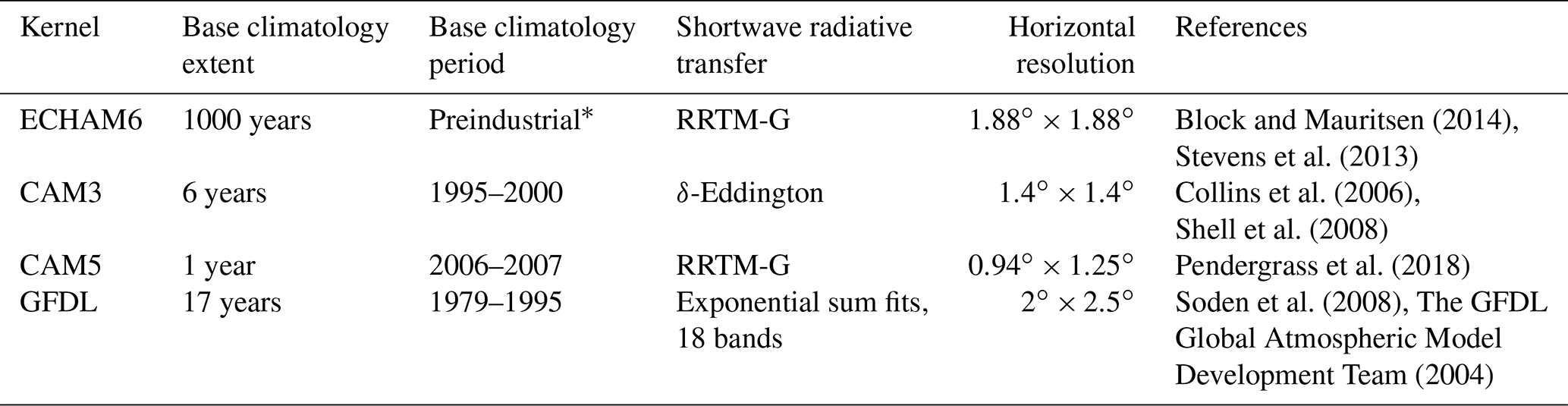
∗ Atmospheric CO2 concentration = 284.7 ppmv; exact time period unknown.
2.2 Single-layer atmosphere models of shortwave radiation transfer
Within the atmospheric science community, various simplified analytical or semiempirical modeling frameworks have been developed, either to diagnose effective surface and atmospheric optical properties from climate model outputs or to study the relative contributions of changes to these properties on shortwave flux changes at the top and bottom of the atmosphere (Atwood et al., 2016; Donohoe and Battisti, 2011; Kashimura et al., 2017; Qu and Hall, 2006; Rasool and Schneider, 1971; Taylor et al., 2007; Winton, 2005, 2006). While these frameworks all treat the atmosphere as a single layer, they differ by whether or not the reflection and transmission properties of this layer are assumed to have a directional dependency (Stephens et al., 2015) and by whether or not inputs other than those derived from the boundary fluxes are required (e.g., cloud properties; Qu and Hall, 2006).
Winton (2005) presented a semiempirical four-parameter optical model to account for the directional dependency of up- and downwelling shortwave fluxes through the one-layer atmosphere and found good agreement (rRMSE <2 % globally) when this was benchmarked to online radiative transfer calculations. Also considering a directional dependency of the atmospheric optical properties, Taylor et al. (2007) presented a two-parameter analytical model where atmospheric absorption was assumed to occur at a level above atmospheric reflection. The analytical model of Donohoe and Battisti (2011) subsequently relaxed the directional dependency assumption and found the atmospheric attenuation of the surface albedo contribution to planetary albedo to be 8 % higher than the model of Taylor et al. (2007). Elsewhere, Qu and Hall (2006) developed an analytical framework making use of additional atmospheric properties such as cloud cover fraction, cloud optical thickness, and the clear-sky planetary albedo, which proved highly accurate when model estimates of planetary albedo were evaluated against climate models and satellite-based datasets.
2.3 Simple empirical parameterizations of the LULCC science community
Two simple empirical parameterizations of shortwave radiative transfer have been widely applied within the LULCC science community for estimating ΔF from Δαs (Bozzi et al., 2015; Caiazzo et al., 2014; Carrer et al., 2018; Cherubini et al., 2012; Lutz et al., 2015; Muñoz et al., 2010). While these parameterizations are also based on a single-layer atmosphere model of shortwave radiative transfer, at the core of these parameterizations is the fundamental assumption that radiative transfer is wholly independent of (or unaffected by) Δαs. In other words, they neglect the change in the attenuating effect of multiple reflections between the surface and the atmosphere that accompanies a change in the surface albedo. Nevertheless, due to their simplicity and ease of application they continue to be widely employed in climate research.
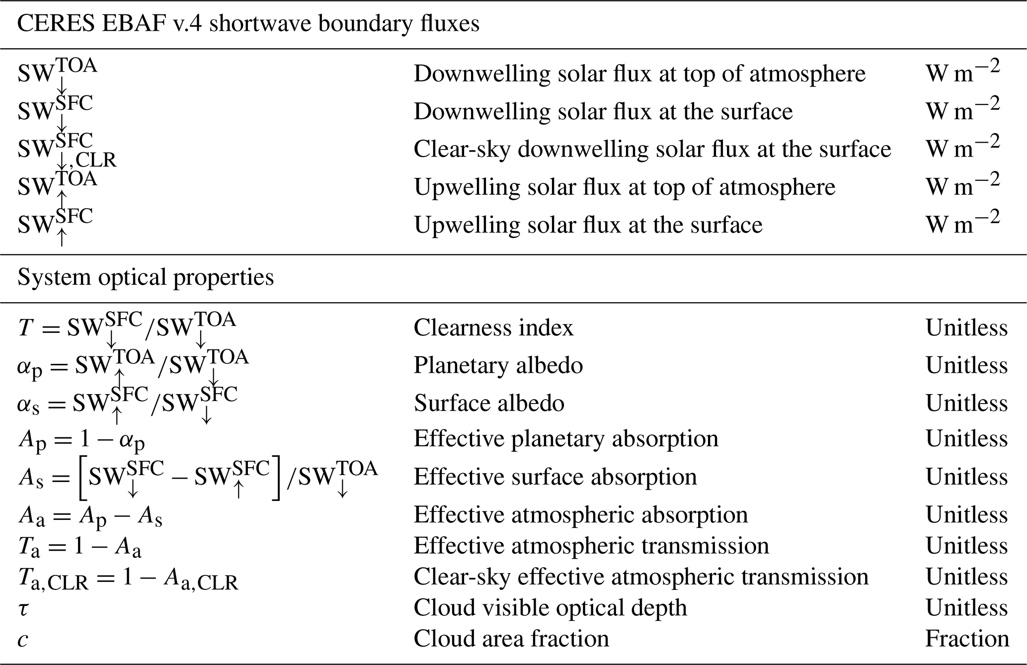
The six candidate models (or parameterizations) for a CERES-based albedo change kernel (CACK) are presented henceforth. All requisite variables and their derivatives may be obtained directly from the CERES EBAF v4 products (at monthly and resolution) and are presented in Table 2. To improve readability, temporal and spatial indexing is neglected and all terms presented henceforth in Sect. 3 denote the monthly pixel means.
Table 2Definition of CERES input variables and other system optical properties derived from CERES inputs. All variables have a monthly temporal resolution and a spatial resolution of .
3.1 Analytical kernels
The first kernel candidate may be analytically derived from the CERES EBAF all-sky boundary fluxes and their derivatives. The surface contribution to the outgoing shortwave flux at TOA can be expressed (Donohoe and Battisti, 2011; Stephens et al., 2015; Winton, 2005) as
where r is a single-pass atmospheric reflection coefficient, a is a single-pass atmospheric absorption coefficient, is the extraterrestrial (downwelling) shortwave flux at TOA, and αs is the surface albedo (defined in Table 2). The expression in the denominator of the right-hand term represents a fraction attenuated by multiple reflections between the surface and the atmosphere. This model assumes that the atmospheric optical properties r and a are insensitive to the origin and direction of shortwave fluxes or – in other words – that they are isotropic.
The single-pass reflectance coefficient is calculated from the system boundary fluxes (Table 2) following Winton (2005) and Kashimura et al. (2017):
while the single-pass absorption coefficient a is given as
where T is the clearness index (defined in Table 2). Our interest is in quantifying the response to an albedo perturbation at the surface – or the partial derivative of with respect to α in Eq. (5):
where is referred to henceforth as the isotropic kernel.
The second analytical kernel is based on the model of Qu and Hall (2006) which makes use of auxiliary cloud property information commonly provided in satellite-based products of Earth's radiation budget – including CERES EBAF – such as cloud cover area fraction, cloud visible optical depth, and clear-sky planetary albedo. This model links all-sky and clear-sky effective atmospheric transmissivities of the earth system through a linear coefficient k relating the logarithm of cloud visible optical depth to the effective all-sky atmospheric transmissivity:
where Ta,CLR is the clear-sky effective system transmissivity, Ta is the all-sky effective system transmissivity, and τ is the cloud visible optical depth. This linear coefficient can then be used together with the cloud cover area fraction to derive a shortwave kernel based on the model of Qu and Hall (2006) – or :
where c is the cloud cover area fraction.
3.2 Semiempirical kernel
The third kernel makes use of three directionally dependent (anisotropic) bulk optical properties r↑, t↑, and t↓, where the first is the atmospheric reflectivity to upwelling shortwave radiation and the latter two are the atmospheric transmission coefficients for upwelling and downwelling shortwave radiation, respectively (Winton, 2005). It is not possible to derive r↑ analytically from the all-sky boundary fluxes; however, Winton (2005) provides an empirical formula relating upwelling reflectivity r↑ to the ratio of all-sky to clear-sky fluxes incident at the surface:
where is the clear-sky shortwave flux incident at the surface.
Knowing r↑, we can then solve for the two remaining optical parameters needed to obtain our kernel:
where Ta is the effective atmospheric transmittance (Table 2) of the earth system.
The kernel may now be expressed as
where is henceforth referred to as the anisotropic kernel.
3.3 Existing empirical parameterizations
Although not referred to as “kernels” in the literature per se, we present the simple empirical parameterizations as such to ensure consistency with previously described notation and terminology.
The first candidate parameterization, originally presented in Muñoz et al. (2010), makes use of a local two-way transmittance factor based on the local clearness index:
where is the local incoming solar flux at TOA, T is the local clearness index, and is the approximated change in the upwelling shortwave flux at TOA due to a change in the surface albedo.
The second candidate parameterization, originally proposed in Cherubini et al. (2012), makes direct use of the solar flux incident at the surface combined with a one-way transmission constant k:
where k is based on the global annual mean share of surface reflected shortwave radiation exiting a clear sky (Lacis and Hansen, 1974; Lenton and Vaughan, 2009) and is hence temporally and spatially invariant. This value – or 0.85 – is similar to the global mean ratio of forward-to-total shortwave scattering reported in Iqbal (1983). Bright and Kvalevåg (2013) evaluated Eq. (16) at several global locations and found large biases for some regions and months, despite good overall performance globally (rRMSE = 7 %; n=120 months).
3.4 Proposed empirical parameterization
To determine whether the GCM-based kernels could be approximated with sufficient fidelity using other simpler model formulations based on their own boundary data, we applied machine learning to identify potential model forms using GCM shortwave boundary fluxes as input. For the two GCMs kernels in which the GCM's own shortwave boundary fluxes are also made available (CAM5 and ECHAM6), we used machine learning to minimize the sum of squared residuals between the four shortwave boundary fluxes (i.e., , , , ) and the GCM kernel at the monthly time step. The reference dataset consisted of a random global sample of 200 000 monthly kernel grid cells at a native model resolution (97 % and 32 % of all cells for ECHAM6 and CAM5, respectively), of which 50 % were used for training and 50 % for validation. Models were identified using a form of genetic programming known as symbolic regression (Eureqa®; Nutonian Inc.; Schmidt and Lipson, 2009, 2010), which searches a wide space of model structures as constrained by user input. In our case, we allowed the model to include the operators (i.e., addition, subtraction, multiplication, division, sine, cosine, tangent, exponential, natural logarithm, factorial, power, square root), but numerical coefficients were forbidden. The model search was allowed to continue until the percent convergence and maturity metrics exceeded 98 % and 50 %, respectively, at which point more than 1×10¹¹ formulae had been evaluated. A parsimonious solution was chosen by minimizing the error metric and model complexity using the Pareto front (Fig. S1 of the Supplement) (Smits and Kotanchek, 2005). Between CAM5 and ECHAM6, four common model solutions were found (Table S1 of the Supplement). The best of these common solutions is subsequently referred to as and is given as
4.1 Initial candidate screening
The four GCM kernels presented in Sect. 2.1 are employed as benchmarks to initially screen the six simple model candidates introduced from Sect. 3.2 to 3.4. We compute a skill metric analogous to the “relative error” metric used to evaluate GCMs by Anav et al. (2013) that takes into account error in the spatial pattern between a model and an observation. Because we have no true observational reference, our evaluation instead focuses on the disagreement or deviation between CERES and GCM kernels at the monthly time step. Given interannual climate variability in the earth system, the challenge of comparing the multiyear CERES kernel to a single-year GCM kernel can be partially overcome by averaging the four GCM kernels.
Using the multi-GCM mean as the reference, we first compute the absolute deviation as
where is the kernel for CERES model candidate x in month m and pixel p and is the multi-GCM mean of the same pixel and month. is then normalized to the maximum absolute deviation of all six CERES kernels for the same pixel and month to obtain a normalized absolute deviation, , which is analogous to the relative error metric of Anav et al. (2013), having values ranging between 0 and 1:
where ) is the maximum absolute deviation of all six CERES kernels at pixel p and month m.
CERES kernel ranking is based on the mean relative absolute deviation in both space and time – or :
where M is the total number of months (i.e., 12) and P is the total number of grid cells.
4.2 GCM kernel emulation
In order to eliminate any bias related to differences in the atmospheric state embedded in the GCM kernel input climatologies, we emulate them by applying the top candidate models (as identified from the initial performance screening described in Sect. 4.1) using the original GCM boundary fluxes as input. Emulation is only done for two of the GCM-based kernels since only two of them have provided the accompanying boundary fluxes needed to do so: ECHAM6 (Block and Mauritsen, 2014) and CAM5 (Pendergrass et al., 2018). Emulation enables a more critical evaluation of the functional form of the candidate models in relation to the more sophisticated radiative transfer schemes employed by ECHAM6 (Stevens et al., 2013) and CAM5 (Hurrell et al., 2013).
4.3 CACK model uncertainty
Following emulation, monthly GCM kernels are then regressed on the monthly kernels emulated with the leading model candidates. The model that best emulates both GCM kernels – as measured in terms of the mean coefficient of determination (R2) and mean RMSE – is chosen to represent CACK.
Three sources of uncertainty are considered for CACK when based on the CERES boundary flux climatology (i.e., 2001–2016 monthly means): (1) physical variability, (2) data uncertainty, and (3) model error (Mahadevan and Sarkar, 2009). The first is related to the interannual variability of Earth's atmospheric state and boundary radiative fluxes. The second is related to the uncertainty of the CERES EBAF v4 variables used as input to CACK (including measurement error). The third source of uncertainty is the error related to CACK's model form. CACK's combined uncertainty for any given pixel and month is estimated as follows, where if CACK or y is some nonlinear function of the CERES boundary inputs x1 and x2 that covary in time and space, then the combined uncertainty of y – or σ(y) – may be expressed as the sum of the model error plus the combined physical variability and data uncertainty associated with x1 and x2 summed in quadrature (Breipohl, 1970; Clifford, 1973; Green et al., 2017):
where σPV(x1) and σPV(x2) are the standard deviations of the 16-year climatological record of CERES input variables x1 and x2, respectively, for a given grid cell and month, σDU (x1) and σDU (x2) are the absolute uncertainties of CERES input variables x1 and x2, respectively, for a given grid cell and month, σ(x1,x2) is the covariance within the 16-year climatological record between CERES input variables x1 and x2 for a given month and grid cell, and σME is the monthly grid cell model error. Model error (σME(y)) and data uncertainties (σDU(xn)) for any given grid cell and month are based on the relative RMSE (Supplement) and relative uncertainties of CERES boundary terms reported in Kato et al. (2018) (cf. Table 8, “Monthly gridded, Ocean + Land”) and Loeb et al. (2017) (cf. Table 8, “All-sky, Terra-Aqua period”). For the model error, we take the relative RMSE of the machine learning model solutions for ECHAM5 and CAM5. For the relative uncertainty of the incoming solar flux at TOA (), we use the 1 % “calibration uncertainty” reported in Loeb et al. (2017).
If CACK's intended application is to estimate a temporally explicit ΔF within the CERES era (i.e., if temporally explicit rather than the climatological-mean CERES boundary fluxes are desired to compute CACK), the uncertainty related to physical variability (σPV(xn)) can be dropped from Eq. (21).
4.4 Climatological CACK application example
To demonstrate CACK's application when based on monthly CERES EBAF climatology, including the handling of uncertainty, we estimate the annual mean local ΔF from a Δαs scenario associated with hypothetical deforestation in the tropics, where ΔF for a given month is estimated as Eq. (4) where is the 2001–2016 monthly climatological CACK and Δαs is the difference in the 2001–2011 monthly climatological-mean white-sky surface albedo between “croplands” (CRO) and “evergreen broadleaved forests” (EBF) taken from Gao et al. (2014), which is based on International Geosphere-Biosphere Program definitions of land cover classification.
The monthly climatological albedo lookup maps of Gao et al. (2014) contain their own uncertainties, which we take as the mean absolute difference between the monthly albedos reconstructed using their lookup model and the monthly MODIS retrieval record (cf. Table 3 in Gao et al., 2014).
The total estimated uncertainty linked to the annual local (i.e., grid cell) instantaneous ΔF can thus be expressed (in W m−2) as
where is the relative grid cell uncertainty of CACK and is the relative uncertainty of Δαs in month m defined as
where σ(αs,m) is the monthly absolute uncertainty of the climatological-mean surface albedo (i.e., of the Gao et al., 2014 product).
4.5 Temporally explicit CACK application example
Use of a temporally explicit CACK may be desirable for time-sensitive applications within the CERES era. This is particularly true for regions experiencing significant changes to the atmospheric state affecting shortwave radiation transfer. A good example is in southern Amazonia where tropical deforestation has been linked to changes in cloud cover (Durieux et al., 2003; Lawrence and Vandecar, 2014; Wright et al., 2017). To exemplify this, we estimate the annual mean instantaneous ΔF for CERES grid cells in the region having experienced both significant positive trends in surface albedo and negative trends in cloud area fraction during the 2001–2016 period. Grid cell trends in surface albedo and cloud area fraction are deemed significant if the slopes of linear fits obtained from local (i.e., grid cell) ordinary least squares regressions have p values ≤0.05. We then apply the slope of the surface albedo trend to represent the monthly mean interannual Δα incurred over the time series together with CACK updated monthly to estimate the local annual mean instantaneous ΔF at each step in the series:
where is the monthly CACK in year t of the time series. ΔF is then averaged across all grid cells in the sample, with the results then compared to the ΔF that is computed for the same grid sample using the time-insensitive CAM5 and ECHAM6 kernels (i.e., ). Using the slope of the surface albedo trend as the Δαs for all months and years rather than the actual Δαs,m(t) (i.e., ) yields the same result when averaged over the full time period but allows us to isolate the effect of the changing atmospheric state on calculations of ΔF. We limit the ΔF uncertainty estimate to CACK's uncertainty that includes σDU(xn) and σME(xn) but excludes σPV(xn).
5.1 Initial performance screening
Seasonally, differences in latitude band means between the CERES kernel candidates and the multi-GCM mean kernels are shown in Fig. 1.
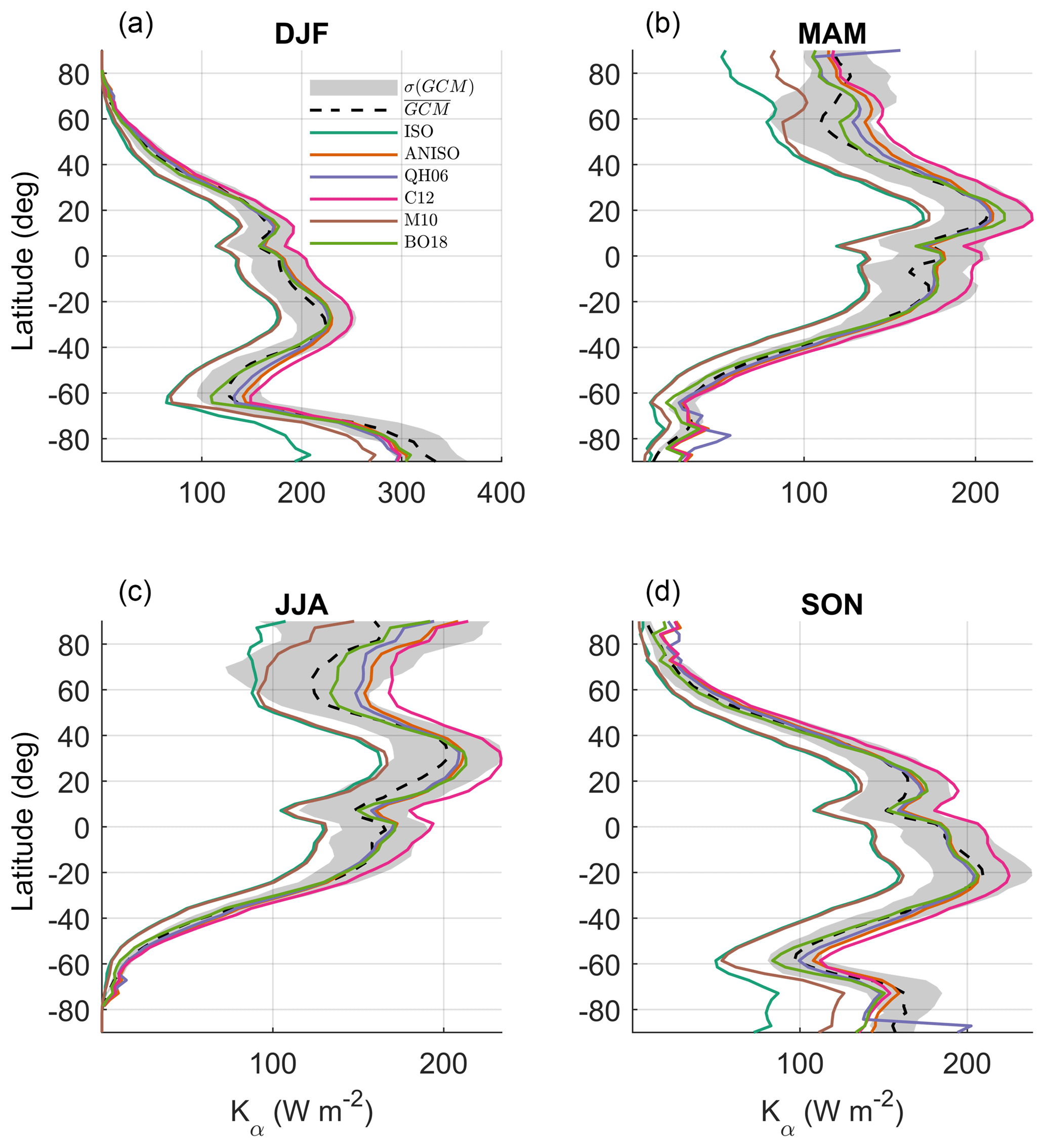
Figure 1Latitudinal (1∘) and seasonal means of the multi-GCM mean () and CACK model candidates for (a) December–January–February (DJF); (b) March–April–May (MAM); (c) June–July–August (JJA); (d) September–October–November (SON). CACK model candidates refer to those presented in Sect. 3 and not to those of the model selection phase of the machine learning algorithm.
Qualitatively, starting with December–January–February (DJF), gives the best agreement with with the exception of the zone around 55–65∘ S (−55 to −65∘), where gives slightly better agreement (Fig. 1a). In March–April–May (MAM), appears to give the best overall agreement with the exception of the high Arctic, where and give better agreement, and with the exception of the zone around 60–65∘ S (−60 to −65∘), where , , and agree best with (Fig. 1b). The largest spread in disagreement across all six CERES kernels is found in June–July–August (JJA; Fig. 1c) at northern high latitudes. appears to agree best both here and elsewhere with the exception of the zone between ∼20–35∘ N, where gives slightly better agreement.
In September–October–November (SON), agrees best with at all latitudes except the zone between 10–25∘ N and 55–65∘ S, where agrees slightly better.
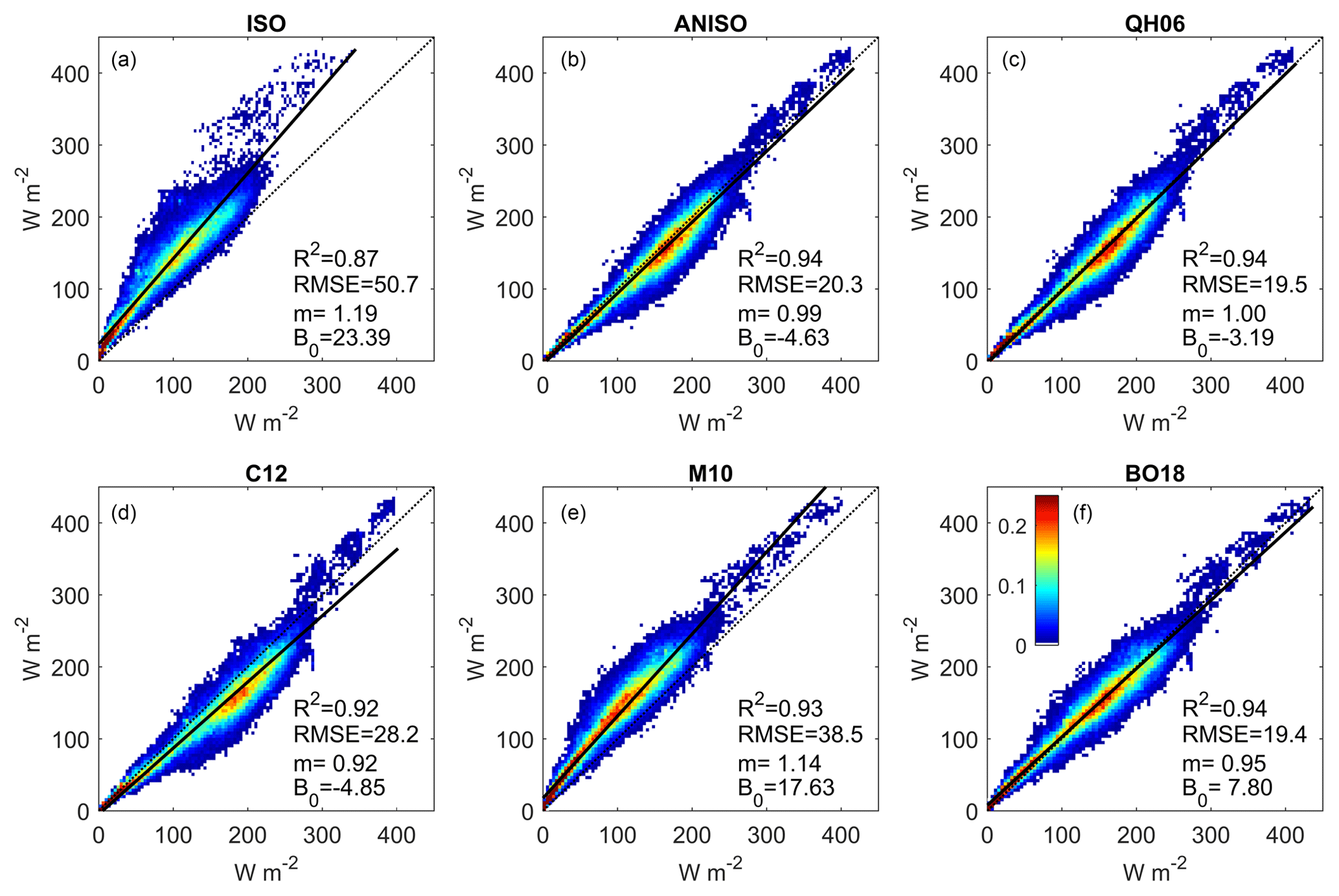
Figure 2(a–f) Scatter–density regressions of global monthly mean (y axis) and (x axis), with the CERES kernel identifier shown at the top of each subpanel. “m”: slope; “B0”: y intercept. The color scale indicates the percentage of regression points that fall within an averaging bin, where the x axis and y axis have been gridded into 100×100 equally spaced bins to help illustrate the density of overlapping points.
Quantitatively, the proportion of the total variance explained by linear regressions of monthly on monthly (i.e., “R2”) is highest and equal for the CERES kernels based on the ANISO, QH06, and BO18 models (Fig. 2b, c, d). Of these three, has a y intercept (“B0”) closest to 0 and a slope (“m”) of 1, although the root mean squared error (“RMSE”) – an accuracy measure – is slightly better (lower) for . The two CERES kernels with the lowest R2, highest slopes (negative deviations), highest RMSEs, and y intercepts with the largest absolute difference from zero – or the worst performing candidates – are those based on the ISO and M10 models (Fig. 2a, e).
Although the y intercept deviation from 0 for is relatively low, its RMSE is ∼50 % higher than that of , , and and leads to notable positive deviation from the multi-GCM mean () judging by its slope of 0.92.
Globally, for the QH06, ANISO, and BO18 kernels is far superior to the ISO, M10, and C12 kernels (Table 3).
Table 3Normalized absolute deviation and CERES kernel model candidate ranking.
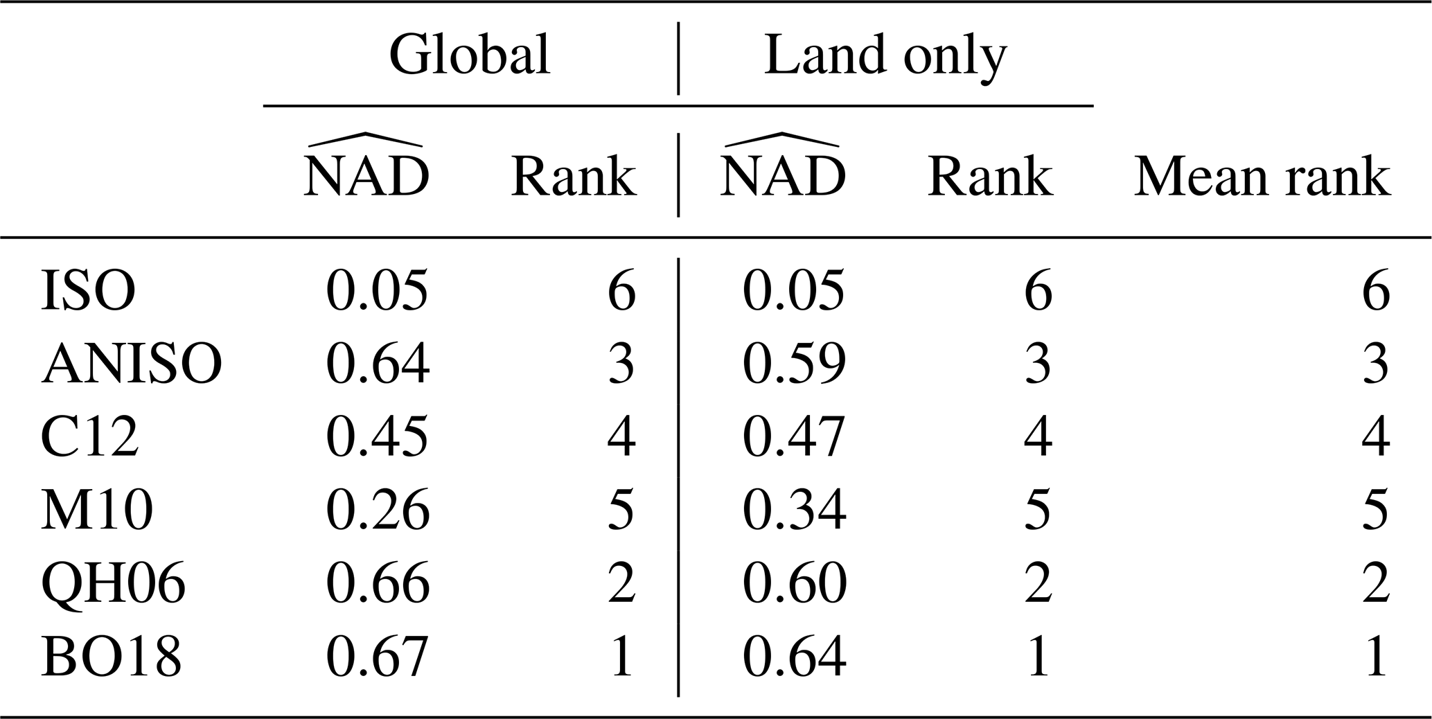
After filtering to remove grid cells for oceans and other water bodies, scores for these three kernels decreased; the decrease was smallest for (−0.03) and largest for (−0.06). Despite constraining the analysis to land surfaces only, the rank order remained unchanged (Table 3), and , , and are subjected to further evaluation.
5.2 GCM kernel emulation and additional performance evaluation
Because the QH06 model () required auxiliary inputs for cloud cover area fraction and cloud optical depth – two atmospheric state variables not provided with the ECHAM6 and CAM5 kernel datasets – it was not possible to emulate these two GCM kernels with . Additional performance evaluation through GCM kernel emulation is therefore restricted to the ANISO and BO18 models.
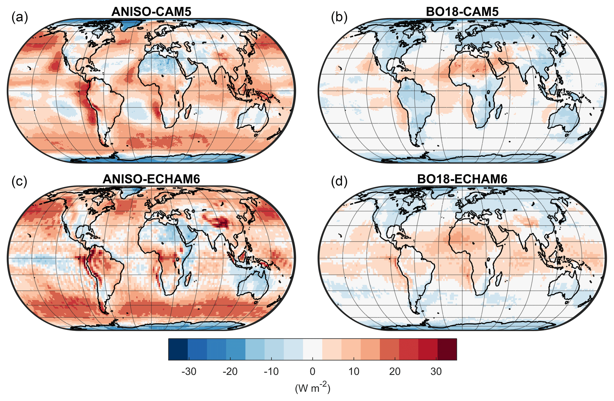
Figure 3(a) Mean annual bias of the CAM5 albedo change kernel emulated with the ANISO semiempirical model; (b) mean annual bias of the CAM5 albedo change kernel emulated with the BO18 parameterization; (c) mean annual bias of the ECHAM6 albedo change kernel emulated with the ANISO semiempirical model; (d) mean annual bias of the ECHAM6 albedo change kernel emulated with the BO18 parameterization.
Globally, the kernel based on the ANISO model displays larger annual mean bias relative to BO18 when compared to both ECHAM6 and CAM5 kernels (Fig. 3). Notable positive biases over land with respect to both ECHAM6 and CAM5 kernels are evident in the northern Andes region of South America, the Tibetan Plateau, and the tropical island region comprising Indonesia, Malaysia, and Papua New Guinea (Fig. 3a, c). Notable negative biases over land with respect to both ECHAM6 and CAM5 kernels are evident over Greenland, Antarctica, northeastern Africa, and the Arabian Peninsula (Fig. 3a, c).
Globally, annual biases for BO18 are generally found to be lower than for ANISO and are mostly non-existent in extra-tropical ocean regions (Fig. 3b, d). Patterns in biases over land are mostly negative with the exception of Saharan Africa where the annual mean bias with respect to both GCMs is positive. For BO18, systematic positive biases – or biases evident with respect to both GCM kernels – appear over eastern tropical and subtropical marine coastal upwelling zones where marine stratocumulus cloud dynamics are difficult for GCMs to resolve (Bretherton et al., 2004; Richter, 2015).
Regression statistics (Fig. 4) indicate a greater overall performance for BO18 than for ANISO. RMSEs for monthly kernels emulated with BO18 are 9.0 and 8.2 W m−2 for CAM5 and ECHAM6, respectively – which is ∼50 %–60 % of the RMSEs emulated with the ANISO model. Relative to ANISO, the BO18 model also gives a higher R2, a slope closer to 1, and a y intercept closer to zero (Fig. 4). The BO18 model (or parameterization) is therefore selected for CACK.
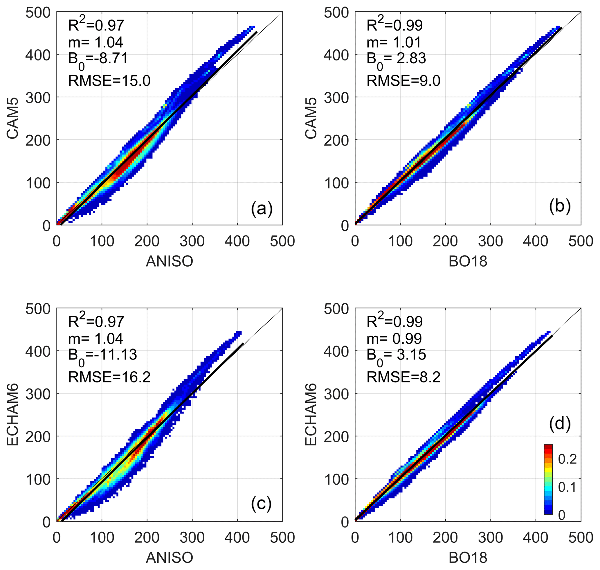
Figure 4(a–d) Scatter–density regressions of (y axis) and emulated with the ANISO semiempirical model and BO18 parameterization using the GCM's own inputs (x axis); “m”: slope; “B0”: y intercept. See Fig. 2 caption for a description of the color scale.
Focusing only on the GCM kernels emulated with henceforth, global mean negative biases are evident in all months (Table 4), with the largest biases (in magnitude) appearing in May (−4.4 W m−2) and November (−2.5 W m−2) for CAM5 and ECHAM6, respectively. In absolute terms, the largest biases of 8.6 and 6.8 W m−2 appear in June for CAM5 and ECHAM6, respectively. Annually, the mean absolute bias for CAM5 and ECHAM6 is 6.8 and 6.1 W m−2, respectively – a magnitude which seems remarkably low if one compares this to the annual mean disagreement (standard deviation) of 33 W m−2 across all four GCM kernels (not shown; for seasonal mean standard deviations, see Fig. 1).
Table 4Global monthly mean bias (MB) and mean absolute bias (MAB) for emulated with T and from ECHAM6 and CAM5. For reference, the global mean value of is 133 W m−2.

5.3 CACK uncertainty
For a kernel based on 2001–2016 monthly mean CERES EBAF climatology, Fig. 5 illustrates the contribution of the absolute error related to 's model form (Fig. 5a, annual mean) relative to CACK's total absolute uncertainty (Fig. 5c, annual mean), which includes the uncertainty surrounding CERES EBAF v4 input variables and and their interannual variability (Fig. 5b, annual mean).

Figure 5Annual uncertainty of a CACK based on 2001–2016 monthly mean CERES EBAF v4 climatology: (a) the absolute uncertainty related to model error (i.e., the parameterization); (b) the total propagated absolute uncertainty related to physical variability and data uncertainty of CACK input variables; (c) total absolute uncertainty; (d) total relative uncertainty.
Total propagated σPV and σDU far exceeds σME, is dominated by and ), and is largest in the Pacific region to the south of the intertropical convergence zone (ITCZ). Over land, the annual σPV and σDU as well as the annual σtotal are generally largest in arid or high-altitude regions (Fig. 5b). However, annual CACK values are also large in these regions, reducing the relative uncertainty (Fig. 5d). The largest relative uncertainties over land (on an annual basis) – which can approach 50 % – are found over central Europe, northwestern Asia, southeastern China, Andean Chile, and northwestern North America (Fig. 5d).
5.4 Climatological CACK application
When estimated with a CACK based on monthly CERES EBAF climatology, the annual local ΔF from Δαs linked to hypothetical deforestation in the tropics is negative in most regions, approaching −20 W m−2 locally in some regions of the Brazilian Cerrado and south of the Sahel region in Africa (Fig. 6b). The combined CACK and Δαs uncertainty for these regions can approach ±5 W m−2 annually (Fig. 6c) in regions like the Brazilian Cerrado and sub-Sahel Africa. Relative to the ΔF magnitude, however, the largest uncertainties (annual) may be found in the subtropical regions of Central America, southern Brazil, southern Asia, and northern Australia, where they can approach 30 %–40 % (Fig. 6d).
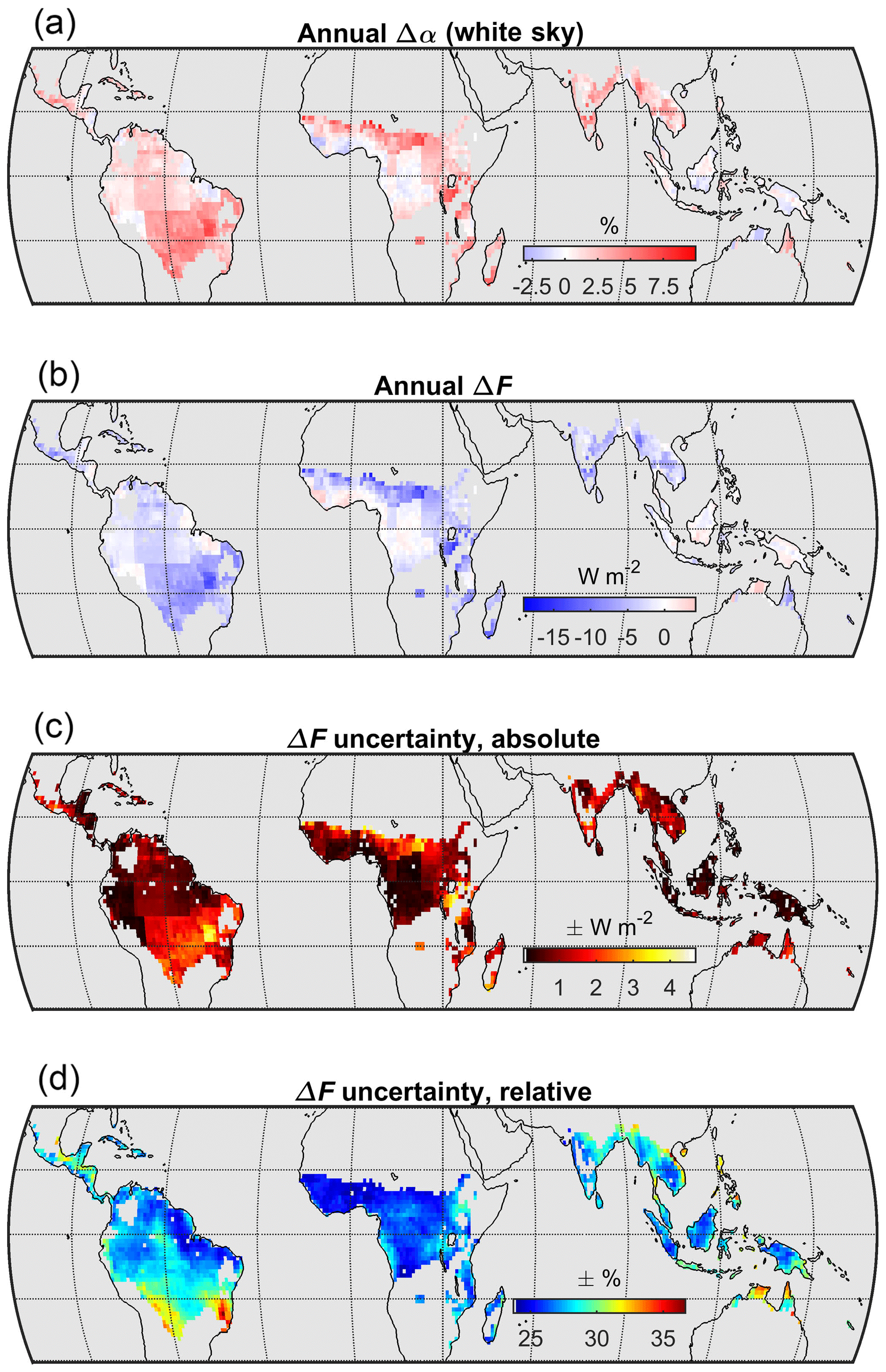
Figure 6Example application of a CACK based on the 2001–2016 monthly mean CERES EBAF v4 climatology to estimate the local annual mean ΔF from a hypothetical land cover change within a CERES grid cell. (a) Annual mean of the climatological (i.e., 2001–2011) monthly mean difference in white-sky surface albedo between croplands and evergreen broadleaved forests (Δαs) based on the 1∘ product of Gao et al. (2014); (b) annual mean local (i.e., within grid cell) instantaneous radiative forcing (ΔF) of monthly mean Δαs estimated with CACK; (c) absolute uncertainty (annual mean) of the CACK-basedΔF estimate, including the uncertainty of Δαs; (d) relative uncertainty (annual mean) of the CACK-based ΔF estimate.
5.5 Temporally explicit CACK application
The effect of a decreasing cloud cover and increasing surface albedo trend in southern Amazonia (Fig. 7b) on shortwave radiative transfer and thus a CACK-based estimate of regional mean annual ΔF emerges in Fig. 7c, where ΔF increases in magnitude by 0.004 W m−2 from 2002 to 2016. This ΔF trend would otherwise go undetected if a GCM-based kernel were applied to the same surface albedo trend – that is, to a sustained positive interannual monthly albedo change “pulse”. Alternatively, a CACK based on 2001 CERES EBAF inputs (applied with Δαs for 2001–2002) would give slightly higher ΔF estimates relative to those based on ECHAM6 and CAM5 kernels; conversely, a CACK based on 2015 CERES EBAF inputs (applied with Δαs for 2015–2016) would yield lower ΔF estimates relative to those based on the same two GCM-based kernels (Fig. 7c). The use of temporally explicit CACK can therefore capture ΔF trends related to a changing atmospheric state that fixed-state GCM kernels are unable to capture.
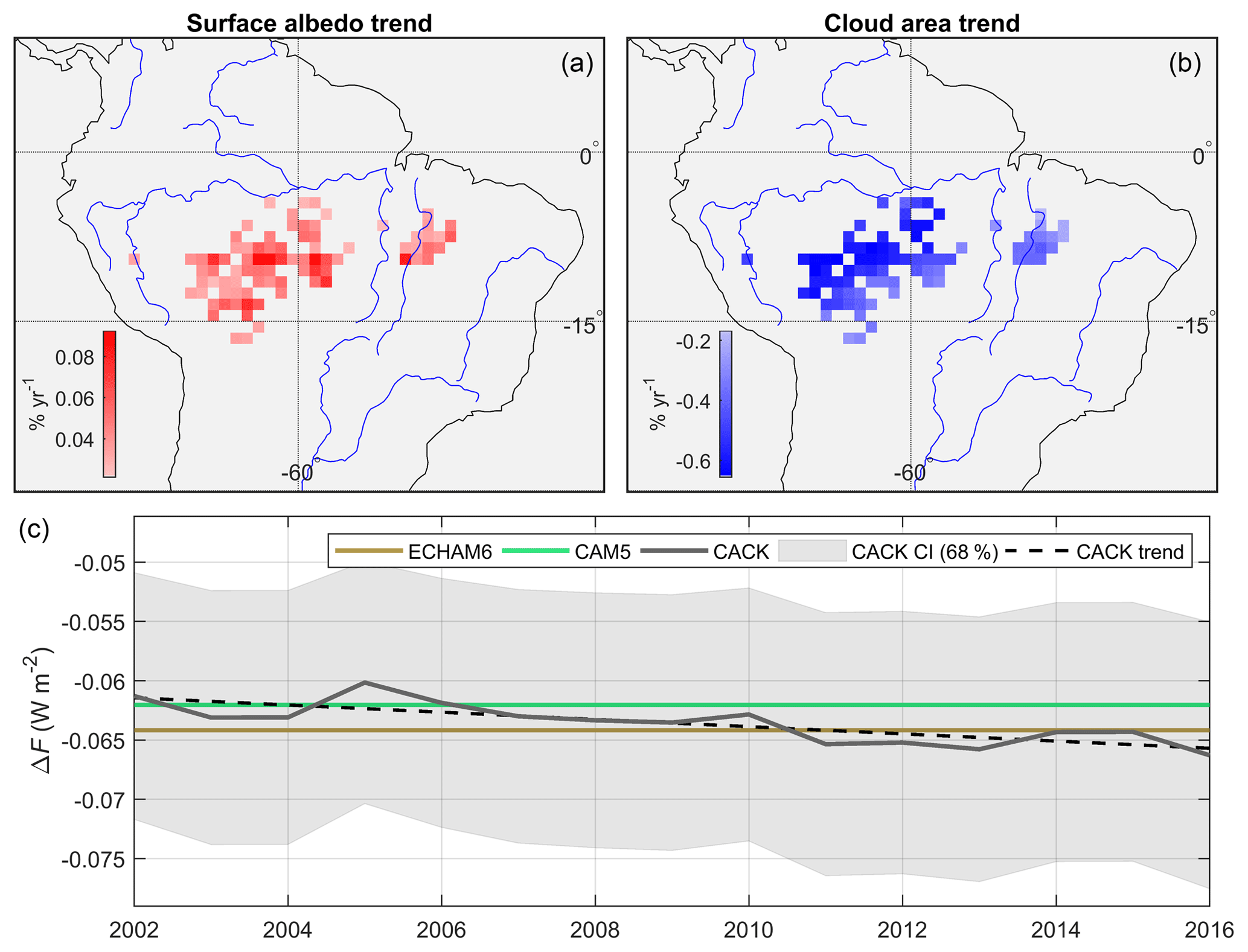
Figure 7Example application of a temporally explicit CACK; (a) 2001–2016 statistically significant positive trends in all-sky surface albedo derived from CERES EBAF-Surface v4; (b) 2001–2016 statistically significant negative trends in cloud area derived from CERES EBAF-TOA v4; (c) mean ΔF from Δαs when estimated with the CACK, ECHAM6, and CAM5 surface albedo change kernels. ΔF is the mean of all grid cells plotted in panel (a). The 1σ confidence interval (“CI”) shown for CACK excludes the uncertainty component related to physical variability.
Motivated by an increasing abundance of climate impact research focusing on land processes in recent years, we comprehensively evaluated six simplified models (or parameterizations) as candidates for an albedo change kernel based on the CERES EBAF v4 products (Kato et al., 2018; Loeb et al., 2017). Relative to albedo change kernels based on sophisticated radiative transfer schemes embedded in GCMs, a CERES-based albedo change kernel – or CACK – represents a more transparent and empirically rooted alternative that can be updated frequently at relatively low cost. This allows greater flexibility to meet the needs of research focusing on surface albedo trends within the CERES era in regions currently undergoing rapid changes to atmospheric state as it affects shortwave radiation transfer. Although some modeling groups have provided recent updates to their albedo change kernels using the latest GCM versions (e.g., Pendergrass et al., 2018), the atmospheric state conditions used to derive them may still be considered outdated or not in sync with that required for many applications (Table 1).
Based on both qualitative and quantitative benchmarking against the mean of four GCM kernels, the novel kernel parameterization obtained from machine learning , together with the two (semi-)analytically derived kernels and , proved far superior to the analytical kernel and to the two additional empirical parameterizations and . When subjected to additional performance evaluation, however, we found that was able to more robustly emulate two GCM kernels (ECHAM6 and CAM5) with exceptionally high agreement, suggesting that could serve as a suitable candidate for CACK.
Relative to the monthly CAM5 and ECHAM6 kernels, the mean absolute monthly emulation “error” of was found to be 6.8 and 6.1 W m−2, respectively – a magnitude which is only ∼20 % of the standard deviation found across four GCM kernels (annual mean). CACK's remarkable simplicity lends support to the idea of using machine learning to explore and detect emergent properties of radiative transfer or other complex, interactive model outputs in future research. The fact that the parameterization emerged as the best common solution from two independently executed machine learning analyses each employing a random sampling unique to a specific GCM kernel suggests that the parameterization is robust and insensitive to the underlying GCM representation of shortwave radiative transfer.
Despite its stronger empirical foundation over a GCM-based kernel, it is important to recognize CACK's limitations. Firstly, while CACK has a finer spatial resolution than most GCM kernels, it still represents a spatially averaged response rather than a truly local response; in other words, the state variables used to define the response are averages tied to the coarse spatial (i.e., ) resolution of the CERES EBAF v4 product grids. Secondly, the monthly CERES EBAF-Surface product used to define lower atmospheric boundary conditions is not strictly an observation. The spaceborne platform is not able to directly observe surface irradiances, requiring additional satellite-based estimates of cloud and aerosol properties as input to a radiative transfer model (Kato et al., 2012). Although TOA irradiances are applied to constrain the surface irradiances, they remain susceptible to errors in the radiative transfer model inputs. Regarding this error as “data uncertainty” increases CACK's overall uncertainty beyond that which is related to its underlying parameterization or “model error”. The uncertainty of CERES surface shortwave irradiances as well as extensive ground validation and testing are documented in greater detail elsewhere (Kato et al., 2013, 2018; Loeb et al., 2017, 2009) and may continue to be reduced in future EBAF-Surface versions.
Concluding remarks
To conclude, we developed, evaluated, and proposed a radiative kernel for surface albedo change based on CERES EBAF v4 products – or CACK. Relative to existing kernels based on GCMs, CACK provides a higher spatial-resolution, higher-transparency alternative that is more amenable to user needs. For LULCC research of the near-past, present-day, or near-future periods, the application of a CACK whose inputs are based on monthly climatological means of the full CERES EBAF record can better account for the corresponding interannual variability in Earth's atmospheric state affecting shortwave radiative transfer. For regions undergoing changes in atmospheric state that are detectable above the normal variability within the CERES era, the application of a temporally explicit CACK can better account for its influence on ΔF estimates from surface albedo change. CACK's input flexibility and transparency combined with documented uncertainty make it well-suited to be applied as part of a monitoring, reporting, and verification (MRV) framework for biogeophysical impacts on land, analogous to those which currently exist for land sector greenhouse gas emissions.
We make both monthly temporally explicit and monthly climatological-mean CACKs for the years 2001–2016 available as a complete data product (“CACKv1.0”; Bright and O'Halloran, 2019) that includes their respective uncertainty layers. A summary of this dataset and associated variables is provided in Table S3 of the Supplement. Octave script files for generating monthly CACK and demonstrating its application with user-specified temporal and spatial extents are bundled with the netCDF file.
CERES EBAF data are available for download at https://ceres.larc.nasa.gov/products.php?product=EBAF-TOA (last access: 5 September 2019, CERES Science Team, 2018a, b). The CAM3 kernel is available at http://people.oregonstate.edu/~shellk/kernel.html (last access: 2 September 2019, Shell, 2008). The CAM5 kernel is available at https://www.earthsystemgrid.org/ac/guest/secure/sso.html (last access: 2 September 2019, Pendergrass, 2017). The ECHAM6 kernel is available at https://swiftbrowser.dkrz.de/public/dkrz_0c07783a-0bdc-4d5e-9f3b-c1b86fac060d/Radiative_kernels/ (last access: 2 September 2019, Block and Mauritsen, 2015).
The supplement related to this article is available online at: https://doi.org/10.5194/gmd-12-3975-2019-supplement.
TLO conceptualized the study. RMB and TLO developed the methodology, curated the data, designed the computer programs, and carried out the formal analysis. TLO and RMB produced the figures. RMB wrote the original draft, and RMB and TLO reviewed and edited the final paper.
The authors declare that they have no conflict of interest.
The authors thank two anonymous reviewers for their constructive comments and feedback.
This research has been supported by the Research Council of Norway (grant nos. 244074/E20 and 250113/F20) and the USDA National Institute of Food and Agriculture (grant no. 2017-68002-26612).
This paper was edited by Rolf Sander and reviewed by two anonymous referees.
Anav, A., Friedlingstein, P., Kidston, M., Bopp, L., Ciais, P., Cox, P., Jones, C., Jung, M., Myneni, R., and Zhu, Z.: Evaluating the Land and Ocean Components of the Global Carbon Cycle in the CMIP5 Earth System Models, J. Climate, 26, 6801–6843, 2013.
Atwood, A. R., Wu, E., Frierson, D. M. W., Battisti, D. S., and Sachs, J. P.: Quantifying Climate Forcings and Feedbacks over the Last Millennium in the CMIP5–PMIP3 Models, J. Climate, 29, 1161–1178, 2016.
Block, K. and Mauritsen, T.: Forcing and feedback in the MPI-ESM-LR coupled model under abruptly quadrupled CO2, J. Adv. Model. Earth Sy., 5, 676–691, 2014.
Block, K. and Mauritsen, T.: ECHAM6 CTRL kernel, available at: https://swiftbrowser.dkrz.de/public/dkrz_0c07783a-0bdc-4d5e-9f3b-c1b86fac060d/Radiative_kernels/ (last access: 2 September 2019), 2015.
Bonan, G. B., Pollard, D., and Thompson, S. L.: Effects of Boreal Forest Vegetation on Global Climate, Nature, 359, 716–718, 1992.
Bozzi, E., Genesio, L., Toscano, P., Pieri, M., and Miglietta, F.: Mimicking biochar-albedo feedback in complex Mediterranean agricultural landscapes, Environ. Res. Lett., 10, 084014, https://doi.org/10.1088/1748-9326/10/8/084014, 2015.
Breipohl, A. M.: Probabilistic systems analysis: an introduction to probabilistic models, decisions, and applications of random processes, Wiley, New York, USA, 1970.
Bretherton, C. S., Uttal, T., Fairall, C. W., Yuter, S. E., Weller, R. A., Baumgardner, D., Comstock, K., Wood, R., and Raga, G. B.: The Epic 2001 Stratocumulus Study, B. Am. Meteorol. Soc., 85, 967–978, 2004.
Bright, R. M.: Metrics for Biogeophysical Climate Forcings from Land Use and Land Cover Changes and Their Inclusion in Life Cycle Assessment: A Critical Review, Environ. Sci. Technol., 49, 3291–3303, 2015.
Bright, R. M. and Kvalevåg, M. M.: Technical Note: Evaluating a simple parameterization of radiative shortwave forcing from surface albedo change, Atmos. Chem. Phys., 13, 11169–11174, https://doi.org/10.5194/acp-13-11169-2013, 2013.
Bright, R. M. and O'Halloran, T. L.: A monthly shortwave radiative forcing kernel for surface albedo change using CERES satellite data, Environmental Data Initiative, https://doi.org/10.6073/pasta/d77b84b11be99ed4d5376d77fe0043d8, 2019.
Caiazzo, F., Malina, R., Staples, M. D., Wolfe, P., J., Yim, S. H. L., and Barrett, S. R. H.: Quantifying the climate impacts of albedo changes due to biofuel production: a comparison with biogeochemical effects, Environ. Res. Lett., 9, 024015, https://doi.org/10.1088/1748-9326/9/2/024015, 2014.
Carrer, D., Pique, G., Ferlicoq, M., Ceamanos, X., and Ceschia, E.: What is the potential of cropland albedo management in the fight against global warming? A case study based on the use of cover crops, Environ. Res. Lett., 13, 044030, https://doi.org/10.1088/1748-9326/aab650, 2018.
CERES Science Team: CERES EBAF-Surface Edition 4.0. NASA Atmospheric Science and Data Center (ASDC), https://doi.org/10.5067/TERRA+AQUA/CERES/EBAF-SURFACE_L3B004.0, 2018a.
CERES Science Team: CERES EBAF-TOA Edition 4.0. NASA Atmospheric Science and Data Center (ASDC), https://doi.org/10.5067/TERRA+AQUA/CERES/EBAF-TOA_L3B004.0, 2018b.
Cherubini, F., Bright, R. M., and Strømman, A. H.: Site-specific global warming potentials of biogenic CO2 for bioenergy: contributions from carbon fluxes and albedo dynamics, Environ. Res. Lett., 7, 045902, https://doi.org/10.1088/1748-9326/7/4/045902, 2012.
Clifford, A. A.: Multivariate error analysis: A handbook of error propagation and calculation in many-parameter systems, Applied Science Publishers, London, UK, 1973.
Collins, W. D., Rasch, P. J., Boville, B. A., Hack, J. J., McCaa, J. R., Williamson, D. L., Briegleb, B. P., Bitz, C. M., Lin, S.-J., and Zhang, M.: The Formulation and Atmospheric Simulation of the Community Atmosphere Model Version 3 (CAM3), J. Climate, 19, 2144–2161, 2006.
Dickinson, R. E. and Henderson-Sellers, A.: Modelling tropical deforestation: A study of GCM land-surface parametrizations, Q. J. Roy. Meteor. Soc., 114, 439–462, 1988.
Dolinar, E. K., Dong, X., Xi, B., Jiang, J. H., and Su, H.: Evaluation of CMIP5 simulated clouds and TOA radiation budgets using NASA satellite observations, Clim. Dynam., 44, 2229–2247, 2015.
Donohoe, A. and Battisti, D. S.: Atmospheric and Surface Contributions to Planetary Albedo, J. Climate, 24, 4402–4418, 2011.
Durieux, L., Machado, L. A. T., and Laurent, H.: The impact of deforestation on cloud cover over the Amazon arc of deforestation, Remote Sens. Environ., 86, 132–140, 2003.
Free, M. and Sun, B.: Trends in U.S. Total Cloud Cover from a Homogeneity-Adjusted Dataset, J. Climate, 27, 4959–4969, 2014.
Gao, F., He, T., Wang, Z., Ghimire, B., Shuai, Y., Masek, J., Schaaf, C., and Williams, C.: Multi-scale climatological albedo look-up maps derived from MODIS BRDF/albedo products, J. Appl. Remote Sens., 8, 083532, https://doi.org/10.1117/1.JRS.8.083532, 2014.
Ghimire, B., Williams, C. A., Masek, J., Gao, F., Wang, Z., Schaaf, C., and He, T.: Global albedo change and radiative cooling from anthropogenic land cover change, 1700 to 2005 based on MODIS, land use harmonization, radiative kernels, and reanalysis, Geophys. Res. Lett., 41, 9087–9096, 2014.
Green, P., Gardiner, T., Medland, D., and Cimini, D.: WP2: Guide to uncertainty in measurement and its nomenclature, Version 4.0., UK, National Physical Laboratory (NPL), Centre for Carbon Measurement, Teddington, UK, 212 pp., 2017.
Hurrell, J. W., Holland, M. M., Gent, P. R., Ghan, S., Kay, J. E., Kushner, P. J., Lamarque, J. F., Large, W. G., Lawrence, D., Lindsay, K., Lipscomb, W. H., Long, M. C., Mahowald, N., Marsh, D. R., Neale, R. B., Rasch, P., Vavrus, S., Vertenstein, M., Bader, D., Collins, W. D., Hack, J. J., Kiehl, J., and Marshall, S.: The Community Earth System Model: A Framework for Collaborative Research, B. Am. Meteorol. Soc., 94, 1339–1360, 2013.
Iqbal, M.: An introduction to solar radiation, Academic Press Canada, Ontario, CA, Canada, 1983.
Jones, A. D., Calvin, K. V., Collins, W. D., and Edmonds, J.: Accounting for radiative forcing from albedo change in future global land-use scenarios, Climatic Change, 131, 691–703, 2015.
Kashimura, H., Abe, M., Watanabe, S., Sekiya, T., Ji, D., Moore, J. C., Cole, J. N. S., and Kravitz, B.: Shortwave radiative forcing, rapid adjustment, and feedback to the surface by sulfate geoengineering: analysis of the Geoengineering Model Intercomparison Project G4 scenario, Atmos. Chem. Phys., 17, 3339–3356, https://doi.org/10.5194/acp-17-3339-2017, 2017.
Kato, S., Loeb, N. G., Rose, F. G., Doelling, D. R., Rutan, D. A., Caldwell, T. E., Yu, L., and Weller, R. A.: Surface Irradiances Consistent with CERES-Derived Top-of-Atmosphere Shortwave and Longwave Irradiances, J. Climate, 26, 2719–2740, 2012.
Kato, S., Loeb, N. G., Rose, F. G., Doelling, D. R., Rutan, D. A., Caldwell, T. E., Yu, L., and Weller, R. A.: Surface irradiances consistent with CERES-derived top-of-atmosphere shortwave and longwave irradiances, J. Climate, 26, 2719–2740, 2013.
Kato, S., Rose, F. G., Rutan, D. A., Thorsen, T. J., Loeb, N. G., Doelling, D. R., Huang, X., Smith, W. L., Su, W., and Ham, S.-H.: Surface Irradiances of Edition 4.0 Clouds and the Earth's Radiant Energy System (CERES) Energy Balanced and Filled (EBAF) Data Product, J. Climate, 31, 4501–4527, 2018.
Lacis, A. A. and Hansen, J. E.: A parameterization for the absorption of solar radiation in the earth's atmosphere, J. Atmos. Sci., 31, 118–133, 1974.
Lawrence, D. and Vandecar, K.: Effects of tropical deforestation on climate and agriculture, Nat. Clim. Change, 5, 27–36, doi:10.1038/nclimate2430, 2014.
Lenton, T. M. and Vaughan, N. E.: The radiative forcing potential of different climate geoengineering options, Atmos. Chem. Phys., 9, 5539–5561, https://doi.org/10.5194/acp-9-5539-2009, 2009.
Li, J. L. F., Waliser, D. E., Stephens, G., Lee, S., L'Ecuyer, T., Kato, S., Loeb, N., and Ma, H.-Y.: Characterizing and understanding radiation budget biases in CMIP3/CMIP5 GCMs, contemporary GCM, and reanalysis, J. Geophys. Res.-Atmos., 118, 8166–8184, 2013.
Loeb, N. G., Wielicki, B. A., Doelling, D. R., Smith, G. L., Keyes, D. F., Kato, S., Manalo-Smith, N., and Wong, T.: Toward optimal closure of the Earth's top-of-atmosphere radiation budget, J. Climate, 22, 748–766, 2009.
Loeb, N. G., Doelling, D. R., Wang, H., Su, W., Nguyen, C., Corbett, J. G., Liang, L., Mitrescu, C., Rose, F. G., and Kato, S.: Clouds and the Earth's Radiant Energy System (CERES) Energy Balanced and Filled (EBAF) Top-of-Atmosphere (TOA) Edition-4.0 Data Product, J. Climate, 31, 895–918, 2017.
Lutz, D. A. and Howarth, R. B.: The price of snow: albedo valuation and a case study for forest management, Environ. Res. Lett., 10, 064013, doi:10.1088/1748-9326/10/6/064013, 2015.
Lutz, D. A., Burakowski, E. A., Murphy, M. B., Borsuk, M. E., Niemiec, R. M., and Howarth, R. B.: Tradeoffs between three forest ecosystem services across the state of New Hampshire, USA: timber, carbon, and albedo, Ecol. Appl., 26, 146–161, 2015.
Mahadevan, S. and Sarkar, S.: Uncertainty analysis methods, U.S. Department of Energy, Washington, D.C., USA, 32 pp., 2009.
Muñoz, I., Campra, P., and Fernández-Alba, A. R.: Including CO2-emission equivalence of changes in land surface albedo in life cycle assessment. Methodology and case study on greenhouse agriculture, Int. J. Life Cycle Ass., 15, 672–681, 2010.
O'Halloran, T. L., Law, B. E., Goulden, M. L., Wang, Z., Barr, J. G., Schaaf, C., Brown, M., Fuentes, J. D., Göckede, M., Black, A., and Engel, V.: Radiative forcing of natural forest disturbances, Glob. Change Biol., 18, 555–565, 2012.
Pendergrass, A. G.: CAM5 Radiative Kernels, available at: https://www.earthsystemgrid.org/dataset/ucar.cgd.ccsm4.cam5-kernels.html (last access: 2 September 2019), 2017.
Pendergrass, A. G., Conley, A., and Vitt, F. M.: Surface and top-of-atmosphere radiative feedback kernels for CESM-CAM5, Earth Syst. Sci. Data, 10, 317–324, https://doi.org/10.5194/essd-10-317-2018, 2018.
Qu, X. and Hall, A.: Assessing Snow Albedo Feedback in Simulated Climate Change, J. Climate, 19, 2617–2630, 2006.
Randerson, J. T., Liu, H., Flanner, M. G., Chambers, S. D., Jin, Y., Hess, P. G., Pfister, G., Mack, M. C., Treseder, K. K., Welp, L. R., Chapin, F. S., Harden, J. W., Goulden, M. L., Lyons, E., Neff, J. C., Schuur, E. A. G., and Zender, C. S.: The Impact of Boreal Forest Fire on Climate Warming, Science, 314, 1130–1132, 2006.
Rasool, S. I. and Schneider, S. H.: Atmospheric Carbon Dioxide and Aerosols: Effects of Large Increases on Global Climate, Science, 173, 138–141, 1971.
Richter, I.: Climate model biases in the eastern tropical oceans: causes, impacts and ways forward, WIRES Clim. Change, 6, 345–358, 2015.
Schmidt, M. and Lipson, H.: Distilling free-form natural laws from experimental data, Science, 324, 81–85, 2009.
Schmidt, M. and Lipson, H.: Symbolic regression of implicit equations, in: Genetic Programming Theory and Practice VII, Springer, doi:10.1007/978-1-4419-1626-6, 2010.
Shell, K. M.: CAM3 radiative kernels, available at: http://people.oregonstate.edu/~shellk/kernel.html (last access: 2 September 2019), 2008.
Shell, K. M., Kiehl, J. T., and Shields, C. A.: Using the Radiative Kernel Technique to Calculate Climate Feedbacks in NCAR's Community Atmospheric Model, J. Climate, 21, 2269–2282, 2008.
Smits, G. F. and Kotanchek, M.: Pareto-front exploitation in symbolic regression, in: Genetic programming theory and practice II, Springer, Boston, USA, 2005.
Soden, B. J., Held, I. M., Colman, R., Shell, K. M., Kiehl, J. T., and Shields, C. A.: Quantifying Climate Feedbacks Using Radiative Kernels, J. Climate, 21, 3504–3520, 2008.
Srivastava, R.: Trends in aerosol optical properties over South Asia, Int. J. Climatol., 37, 371–380, 2017.
Stephens, G. L., O'Brien, D., Webster, P. J., Pilewski, P., Kato, S., and Li, J.-l.: The albedo of Earth, Rev. Geophys., 53, 141–163, 2015.
Stevens, B., Giorgetta, M., Esch, M., Mauritsen, T., Crueger, T., Rast, S., Salzmann, M., Schmidt, H., Bader, J., Block, K., Brokopf, R., Fast, I., Kinne, S., Kornblueh, L., Lohmann, U., Pincus, R., Reichler, T., and Roeckner, E.: Atmospheric component of the MPI-M Earth System Model: ECHAM6, J. Adv. Model. Earth Sy., 5, 146–172, 2013.
Taylor, K. E., Crucifix, M., Braconnot, P., Hewitt, C. D., Doutriaux, C., Broccoli, A. J., Mitchell, J. F. B., and Webb, M. J.: Estimating Shortwave Radiative Forcing and Response in Climate Models, J. Climate, 20, 2530–2543, 2007.
The GFDL Global Atmospheric Model Development Team: The New GFDL Global Atmosphere and Land Model AM2–LM2: Evaluation with Prescribed SST Simulations, J. Climate, 17, 4641–4673, 2004.
Vanderhoof, M., Williams, C. A., Ghimire, B., and Rogan, J.: Impact of mountain pine beetle outbreaks on forest albedo and radiative forcing, as derived from Moderate Resolution Imaging Spectroradiometer, Rocky Mountains, USA, J. Geophys. Res.-Biogeo., 118, 1461–1471, 2013.
Wang, H. and Su, W.: Evaluating and understanding top of the atmosphere cloud radiative effects in Intergovernmental Panel on Climate Change (IPCC) Fifth Assessment Report (AR5) Coupled Model Intercomparison Project Phase 5 (CMIP5) models using satellite observations, J. Geophys. Res.-Atmos., 118, 683–699, 2013.
Winton, M.: Simple optical models for diagnosing surface-atmosphere shortwave interactions, J. Climate, 18, 3796–3806, 2005.
Winton, M.: Surface Albedo Feedback Estimates for the AR4 Climate Models, J. Climate, 19, 359–365, 2006.
Wright, J. S., Fu, R., Worden, J. R., Chakraborty, S., Clinton, N. E., Risi, C., Sun, Y., and Yin, L.: Rainforest-initiated wet season onset over the southern Amazon, P. Natl. Acad. Sci. USA, 114, 8481–8486, https://doi.org/10.1073/pnas.1621516114, 2017.
Zhao, D., Xin, J., Gong, C., Wang, X., Ma, Y., and Ma, Y.: Trends of Aerosol Optical Properties over the Heavy Industrial Zone of Northeastern Asia in the Past Decade (2004–15), J. Atmos. Sci., 75, 1741–1754, 2018.