the Creative Commons Attribution 4.0 License.
the Creative Commons Attribution 4.0 License.
 | 23 Sep 2019
Identification of key parameters controlling demographically structured vegetation dynamics in a land surface model: CLM4.5(FATES)
Elias C. Massoud
Chonggang Xu
Rosie A. Fisher
Ryan G. Knox
Anthony P. Walker
Shawn P. Serbin
Bradley O. Christoffersen
Jennifer A. Holm
Lara M. Kueppers
Daniel M. Ricciuto
Liang Wei
Daniel J. Johnson
Jeffrey Q. Chambers
Charlie D. Koven
Nate G. McDowell
Jasper A. Vrugt
Vegetation plays an important role in regulating global carbon cycles and is a key component of the Earth system models (ESMs) that aim to project Earth's future climate. In the last decade, the vegetation component within ESMs has witnessed great progress from simple “big-leaf” approaches to demographically structured approaches, which have a better representation of plant size, canopy structure, and disturbances. These demographically structured vegetation models typically have a large number of input parameters, and sensitivity analysis is needed to quantify the impact of each parameter on the model outputs for a better understanding of model behavior. In this study, we conducted a comprehensive sensitivity analysis to diagnose the Community Land Model coupled to the Functionally Assembled Terrestrial Simulator, or CLM4.5(FATES). Specifically, we quantified the first- and second-order sensitivities of the model parameters to outputs that represent simulated growth and mortality as well as carbon fluxes and stocks for a tropical site with an extent of 1×1∘. While the photosynthetic capacity parameter (Vc,max25) is found to be important for simulated carbon stocks and fluxes, we also show the importance of carbon storage and allometry parameters, which determine survival and growth strategies within the model. The parameter sensitivity changes with different sizes of trees and climate conditions. The results of this study highlight the importance of understanding the dynamics of the next generation of demographically enabled vegetation models within ESMs to improve model parameterization and structure for better model fidelity.


Earth system models (ESMs) are abstract representations of nature used to simulate physical, chemical, and biological processes across the interacting domains of the Earth system to estimate past, present, and future climate (Claussen et al., 2002; Dunne et al., 2012; Arora et al., 2013; Hurrell et al., 2013). Land surface models (LSMs), the land component of ESMs, are capable of representing vegetation dynamics through the use of dynamic global vegetation models (Foley et al., 1996; Cox et al., 2000; Krinner et al., 2005; Friedlingstein et al., 2006; Sato et al., 2007; Arora et al., 2013). The first-generation dynamic vegetation models represent plant communities and their competition using a single area-averaged representation of plant functional types (PFTs) within each land grid cell (Cox et al., 2000; Pan et al., 2002; Hickler et al., 2004). Recently, a number of vegetation models that can represent plant demographic processes have emerged to better capture coexistence and competition driven by light competition between different sizes of trees within a vertical canopy structure at different successional stages (Moorcroft et al., 2001; Thonicke et al., 2001; Sitch et al., 2003; Hickler et al., 2004; Fisher et al., 2010; Scheiter et al., 2013; Fisher et al., 2018). These demographic models allow comparison with many more observed vegetation processes than first-generation models but also contain more degrees of freedom leading to great complexity.
LSMs typically contain a suite of different parameters to resolve the carbon, water, and energy fluxes and pools at the land–atmosphere interface (Noilhan and Planton, 1989; Bastidas et al., 1999; Gupta et al., 1999; Masson et al., 2003; Sargsyan et al., 2014). Many of these parameters can be estimated directly in the field, but others are difficult or impossible to measure due to various complications such as the abstract representation of processes, technological limitations, or spatial/temporal aggregation (Entekhabi and Eagleson, 1989; Kumar et al., 2006). Parameters that are observable in the field are also often subject to large natural variability, including changes through space and time (Wood et al., 1992; Masson et al., 2003; Fisher et al., 2015). For example, vegetation parameters can be used to describe different root profiles (Vrugt et al., 2001; Zeng, 2001; Massoud et al., 2019a) or photosynthetic capacities (Leuning, 2002; Rogers, 2014); however, model parameter values are often taken from literature publications or databases, and may not represent local variation or capture seasonal or ontogenetic changes. For parameters of critical importance, even a small difference can lead to significant divergence for multi-model ensemble projections or uncertainty in model predictions from different models (Sitch et al., 2008; Dietze et al., 2014; McDowell et al., 2016; Rogers et al., 2017). Since parameters are often defined in simulations with limited prior knowledge of their mean values and variation (O'Hagan and Leonard, 1976; Kitanidis, 1986; Geromel, 1999), model uncertainty or sensitivity analyses are typically required to adequately quantify the uncertainty in model outputs and importance of parameters to guide model calibration and improvement.
There are two types of uncertainty and sensitivity analysis studies. One type of study aims to understand the model behaviors by exploring the baseline sensitivity of model outputs to parameter changes, which is normally an equal amount of deviation from the mean values of default parameters. This is commonly referred to as model sensitivity or elasticity analysis (e.g., Benton and Grant, 1999; Pappas et al., 2013; Menberg et al., 2016; Collalti et al., 2019). Another type of study aims to quantify the amount of uncertainty in model outputs and the corresponding contributions to this uncertainty by different sources, which is commonly referred to as uncertainty quantification (e.g., Xu et al., 2010; Dietze et al., 2014). It is possible that a model output is very sensitive to a particular parameter in the sensitivity analysis study, but the parameter could contribute to a small amount of uncertainty in the model output if this parameter contains a low level of variation (Dietze et al., 2014). Both types of studies are useful for model development and applications with sensitivity analysis studies focusing on understanding the baseline of model behaviors and uncertainty quantification studies focusing on guiding field and laboratory measurements. Despite the need for such studies, systematic investigation of the parameter sensitivity and output uncertainty of LSMs is not standard practice, potentially on account of the high dimensionality involved (although see Zaehle et al., 2005; Fisher et al., 2010; Pappas et al., 2013).
Today, many uncertainty and sensitivity analysis techniques are available (Sobol', 1990; Helton, 1993; Saltelli et al., 2000; Razavi and Gupta, 2016). Some of these methods examine the response of the outputs by varying input parameters one at a time and holding other parameters at their default values (Saltelli et al., 2000). However, the sensitivity index derived by this type of assessment depends on the default values of the other parameters, and the assumption that these values are satisfactory is questionable (e.g., Da Rocha et al., 1996; Sen et al., 2001; Groenendijk et al., 2011; Schwalm et al., 2010) since the LSM predictions are strongly tied (through feedbacks of momentum, energy, mass, and biogeochemistry) to the differences in their representation of the land surface (Crossley et al., 2000; Rosolem et al., 2013). Therefore, it is desirable to use more extensive sensitivity analysis techniques that examine the response of model outputs averaged over the variation of all the parameters. These “global” methods are generally preferred when computing power is not a limiting factor, as they require a relatively large number of ensemble runs. A sensitivity analysis is considered to be global when all the input factors are varied simultaneously and the sensitivity is evaluated over their entire range of interest (McRae et al., 2001; Xu and Gertner, 2008; Zhou et al., 2008). For sensitivity analysis studies, the entire range of interest could be a certain percentage deviation of default values of parameters. For uncertainty quantification studies, the entire range of interest could be the distributions of parameters estimated from laboratory measurements, field observations, and expert knowledge. Campolongo et al. (2000) suggested classifying local and global sensitivity analysis based largely on the extent of the input variable range that the technique assesses; however, this classification is ambiguous, as it depends on whether the range is sufficiently large to be perceived as global (Song et al., 2015).
The goal of this study is to conduct a comprehensive sensitivity analysis for a land surface model (Community Land Model) coupled to a demographic vegetation model (Functionally Assembled Terrestrial Simulator), or CLM4.5(FATES), at a tropical site with an extent of 1×1∘ to (1) understand the baseline model behaviors of vegetation carbon stocks and fluxes and vegetation demography in relation to different model parameters, and (2) provide directions for improved model parameterization toward a better model fit to observations. Specifically, we aim to answer the following question: what are the main parameter controls on vegetation processes such as growth and mortality and on the resulting dynamics of carbon fluxes and stocks? Based on our understanding of simulated processes in CLM4.5(FATES), we propose to test three hypotheses. Our first hypothesis is related to photosynthetic capacity. The carbon input for vegetation growth is through photosynthesis and in most LSMs, it is simulated based on the Farquhar model (Farquhar, 1989) with the photosynthetic capacity represented by the maximum carboxylation rate at 25 ∘C (Vc,max25) and maximum electron transport rate at 25 ∘C (Jmax25). Jmax25 is simulated in proportion to Vc,max25 in many models, and previous sensitivity analysis studies (Pappas et al., 2013; Sargsyan et al., 2014; Dietze et al., 2014) have shown that Vc,max25 is generally an important parameter that affects simulated carbon fluxes. Therefore, we hypothesize that the photosynthetic capacity parameter, Vc,max25, is a key control on simulated carbon fluxes in CLM4.5(FATES) (H1). Second, for demographic models, the allometry of trees determines the amount of carbon input to different tissues (e.g., leaf, root, and stem). If more carbon is allocated to leaf compared to stem, the tree will have a higher productivity but this can also lead to lower stem growth and thus less height growth for light competition. Thus, we hypothesize that allometry parameters are important for vegetation growth and long-term carton stocks (H2), as they will determine plant's growth strategies. Finally, the carbon stock for vegetation is affected not only by the input of carbon through photosynthesis but also by the loss of carbon through mortality. We hypothesize that the parameters determining mortality are important drivers of the long-term vegetation carbon stocks (H3), as they will control carbon turnover time.
2.1 CLM4.5(FATES)
CLM4.5(FATES) is an open-source land surface model coupled with a demographically structured dynamic vegetation model designed to predict climate–vegetation interactions. The land surface Community Land Model (CLM) represents surface heterogeneity and simulates land biogeophysics, the hydrologic cycle, biogeochemistry, human dimensions, and ecosystem dynamics (Oleson et al., 2013). It is used within various Earth system modeling frameworks, including the Community Earth System Model (CESM) and the Norwegian Earth System Model (NorESM) (Lawrence et al., 2011; Bonan et al., 2011). It is also the baseline of the land component within the Exascale Energy Earth System Model (E3SM) (Golaz et al., 2019). The vegetation model FATES is developed from the ecosystem demography (ED) model, which scales up the behavior of forest ecosystems by aggregating individual trees into representative “cohorts” based on their size and PFT, and by aggregating groups of cohorts into representative “patches” (conceptually similar to a forest plot) that explicitly tracks the time between disturbances (Moorcroft et al., 2001). The main property of the ED concept that differs from most commonly used “big-leaf” models is the capacity to predict distribution, structure, and composition of vegetation directly from their given physiological traits described by the model parameterization (Fisher et al., 2015). This is achieved via the means of trait filtering, whereby plant traits affect plant growth and survival, growth in turn affects the acquisition of light resources, and feeds back onto growth, survival, and reproduction. Differences in growth, survival, and reproduction rates thus directly control the relative distributions of vegetation types and their traits as well as the overall carbon stocks. See supplementary model description in Fisher et al. (2015) for details on specific components of the model structure. FATES represents vegetation using size-structured groups of plants (cohorts) which coexist on various successional trajectory-based land units. FATES simulates growth by integrating photosynthesis across different leaf layers for each cohort. The model allocates photosynthetic carbon to different tissues such as leaf, root, and stem based on the allometry of different vegetation types. Mortality is an important driver for the simulated forest dynamics in FATES. FATES includes five modes of mortality: (1) fixed background mortality, (2) hydraulic failure based on a threshold of very low soil moisture; (3) carbon starvation resulting from the depletion of carbon storage in plants (see Appendix C for details); (4) impact mortality resulting from the falling of big trees; and (5) fire (Fisher et al., 2015). CLM and FATES are coupled to exchange carbon and water between vegetation and soil through a common interface. FATES is designed to be modular and currently can be turned on within two land surface models: the CLM and E3SM land model (ELM). Depending on the purpose of different studies, CLM4.5(FATES) can be simulated with different modes including point mode for individual sites, regional mode for watershed or regional scales, and global mode for the global scale.
In this original version of CLM4.5(FATES), there are two challenges for the model to simulate tropical forests. First, it is difficult for the model to represent the coexistence of PFTs due to the dominance of growth and reproductive feedbacks and potentially the absence of additional stabilizing mechanisms (Fisher et al., 2010, 2018); therefore, in this initial analysis, we focus only on a single broadleaf evergreen tree PFT, which is a typical vegetation type for the study region (the Amazon). We want to point out that, because of the high species diversity in the tropics, it is always a challenge for models to capture diverse traits with a limited number of PFTs in typical ESMs. By limiting our sensitivity analysis to one PFT in this study, our sensitivity analysis will help us understand the main control on demographic rates of growth and mortality that will essentially affect the outcome of competition for multiple PFTs. Thus, we expect that our sensitivity analysis can be used to guide the selection of traits for the representation of trait trade-off for diverse tropical forests and to improve the simulation of PFT coexistence for model calibration and improvement. Second, the model generally underestimates leaf area index (LAI). We expect that our sensitivity analysis will be used as a guidance to adjust identified key model parameters in order to better fit model predictions to the observations.
The CLM4.5(FATES) tracks different size classes of plants (generally >10 size classes) through time. To facilitate our analysis, we aggregate cohorts into three size categories: small (<10 cm), medium (10–50 cm), and large trees (>50 cm). For sensitivity analysis of each size category (small, medium, and large trees), we choose to average the outputs over 30-year intervals. This is done with the view that a large amount of variability in model outputs could be caused by the transient and abrupt changes across size classes, and thus only a small amount of variability is affected by parametric variations. Our analysis shows that the identified key parameters and the corresponding magnitude of sensitivity are similar with averaging over different numbers of years from 20 to 40 years (Fig. D1).
2.2 Sensitivity analysis: the FAST method
Global sensitivity analysis aims at quantifying the contributions of input variables to the variability of the outputs of a physical model by simultaneously sampling values of parameters from their corresponding statistical distributions. There are many methods for global sensitivity analysis. Two popular variance-based approaches are the Sobol method (Sobol', 1990) and the Fourier amplitude sensitivity test (FAST) (Cukier et al., 1973). The Sobol method has received much attention since it provides a clear description of the importance index of model parameters based on variance decomposition. However, the full description requires the evaluation of 2n Monte Carlo integrals (Sudret, 2008), which is not practically feasible unless n is low (n here represents the dimensionality of the model or the number of active parameters). Compared to Sobol's method, FAST is more computationally efficient. It can be used effectively for nonlinear and nonmonotonic models (Sudret, 2008; Xu and Gertner, 2011a). FAST uses a periodic sampling approach to draw samples from the parameter space defined by probability distributions with a characteristic periodic signal for each parameter. These samples will then be fed into the model for ensemble simulations. Finally, a Fourier transformation is applied to decompose the variance of a model output into partial variances contributed by different model parameters based on the characteristic periodic signal assigned for each parameter. Only the first-order sensitivity indices referring to the “main effect” of parameters were calculated in the original method. In the 1990s, an extended FAST method able to calculate sensitivity indices referring to “total effect” was developed (Sobol', 1990; Archer et al., 1997; Saltelli et al., 1999). This “total effect” of a parameter's sensitivity refers to the sum of a parameter's individual contribution (first-order sensitivity) and the contribution from its interaction with other parameters (higher-order sensitivity) on the overall variance of the model output; that is, the total effect includes all the higher-order interactions. Xu and Gertner (2011a) further derived equations within the FAST framework to calculate specific higher-order interactions for different sampling approaches. The FAST method has found widespread use in many different fields of study including sensitivity analysis of the parameters of models that represent the land surface (Collins and Avissar, 1994), chemical reaction (Haaker and Verheijen, 2004), nuclear waste disposal (Lu and Mohanty, 2001), erosion (Wang et al., 2001), hydrologic systems (Francos et al., 2003), atmospheric systems (Kioutsioukis et al., 2004), crop growth (Wang et al., 2013), or matrix population and forest landscape models (Xu and Gertner, 2009; Xu et al., 2009).
In this study, we quantify both the first- and second-order sensitivities of the model parameters using FAST. It is possible to identify higher-order interactions with FAST; however, because of the sample size limitations for a larger trivariate parameter space, the FAST-based estimation of third-order sensitivity indices would be less reliable (Xu and Gertner, 2011a). Specifically, the first-order sensitivity is used to measure the importance of the variations in one parameter to the model outputs. If one parameter xi is important to a model output y at time t (i.e., y(t)), we expect that the mean value of y(t) will change substantially with different values of xi. Statistically, we expect to see a large variance of the expected value of y(t) given xi (i.e., large V(E(y(t)|xi)), where E(⋅) is the expected value of the output, V(⋅) is the variance calculated in the parameter space). Similarly, if the combined impact of xi and xj is important, we expect to see a large variance of the expected value of y(t) given xi and xj (i.e., large V(E(y(t)|xi,xj))). Therefore, we calculate the first- and second-order sensitivities, and , respectively, of the model parameters for each output of interest and at each time step as follows:
where V(y(t)) is the total variance of model output y(t). In FAST, the variances are estimated through periodic samples in the θ space between 0 and 2π, which are linked to the samples in the parameter space through a search function. Further details on the FAST toolbox used for this study can be found in Xu and Gertner (2007, 2009, 2011a) or Xu et al. (2009). We are aware that FAST can provide robust estimates of the sensitivity coefficients in high dimensions (Wang et al., 2013), especially since the CPU demands of CLM4.5(FATES) mandates application of a method like FAST due to its ability to derive sensitivity values with sparse sampling. Due to the random parametric sampling, there will be errors in the estimates of sensitivity indices. In this study, we estimate the standard error of FAST-based sensitivity index derived by Xu and Gertner (2011b), with lower errors for a larger sample size.
To better understand how parameters affect specific CLM4.5(FATES) output variables (i.e., the relationship between model parameters and outputs), we also fitted cubic splines to the scatterplots between samples of parameters identified as important by FAST and the corresponding output variable of interest using the R SemiPar package (Ruppert et al., 2003).
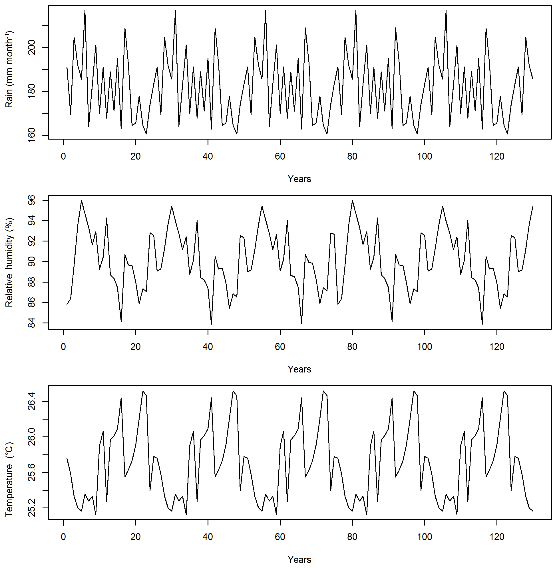
Figure 1Recycled climate drivers for the study area including annual mean precipitation, relative humidity, and air temperature for the years 1948–1972. The annual radiation and air pressure are not plotted as they are quite stable across years.
2.3 Parameter selection
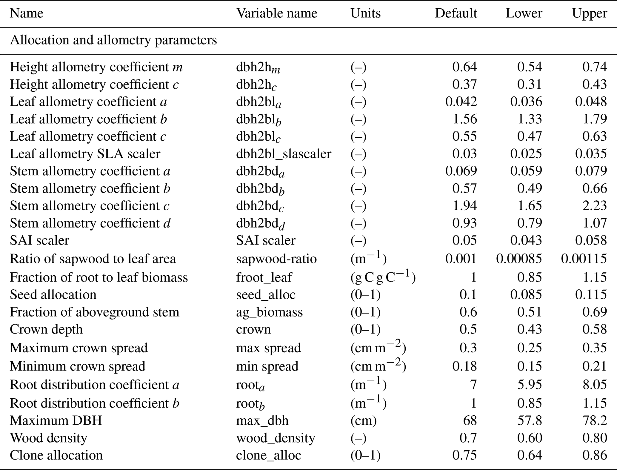
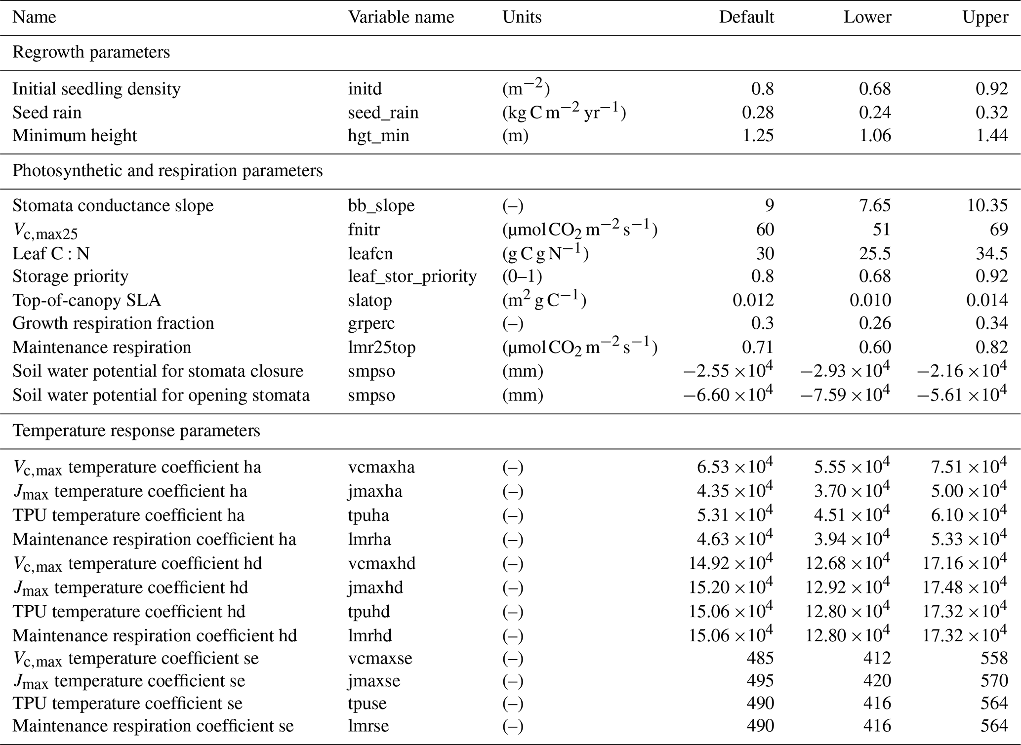
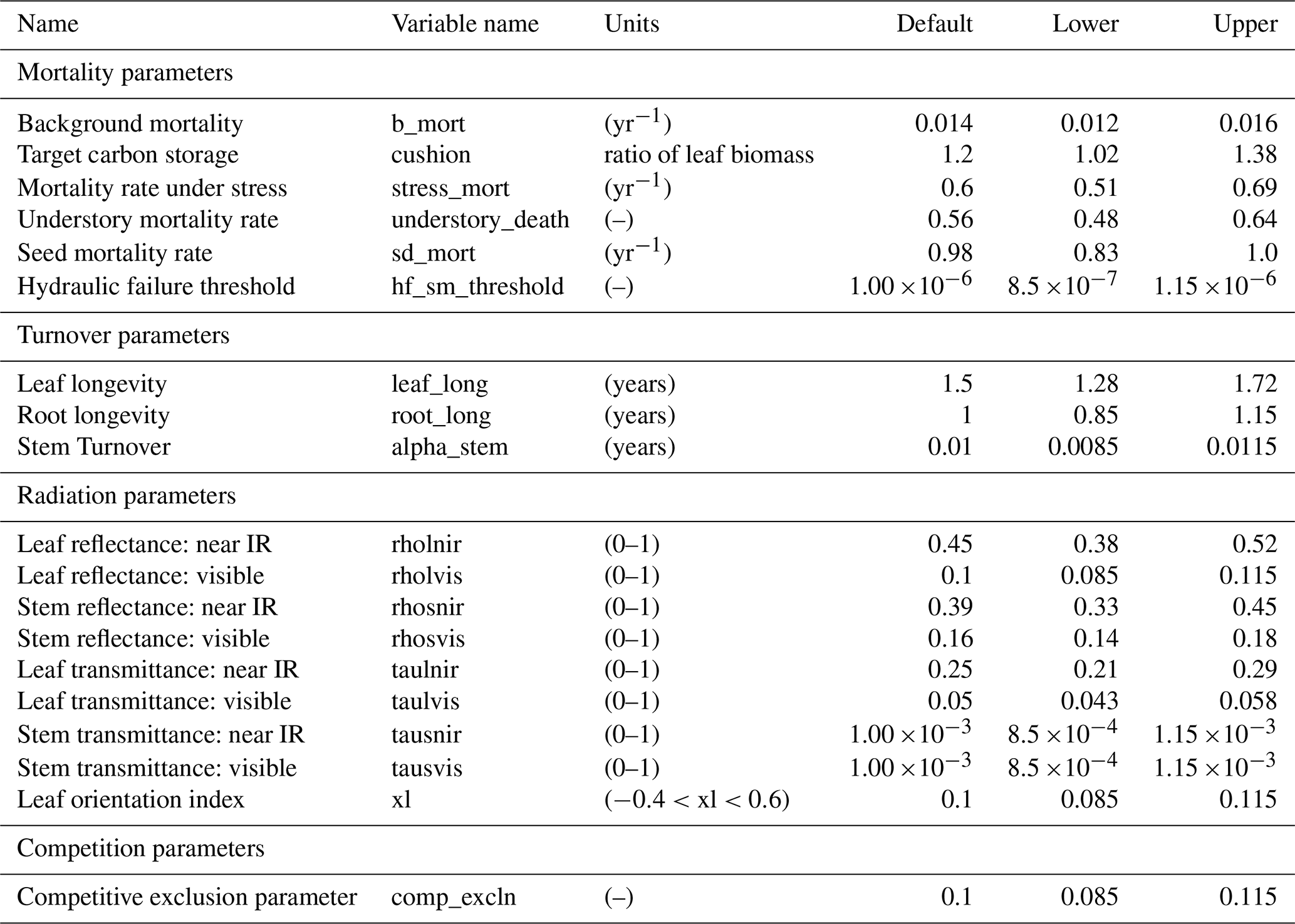
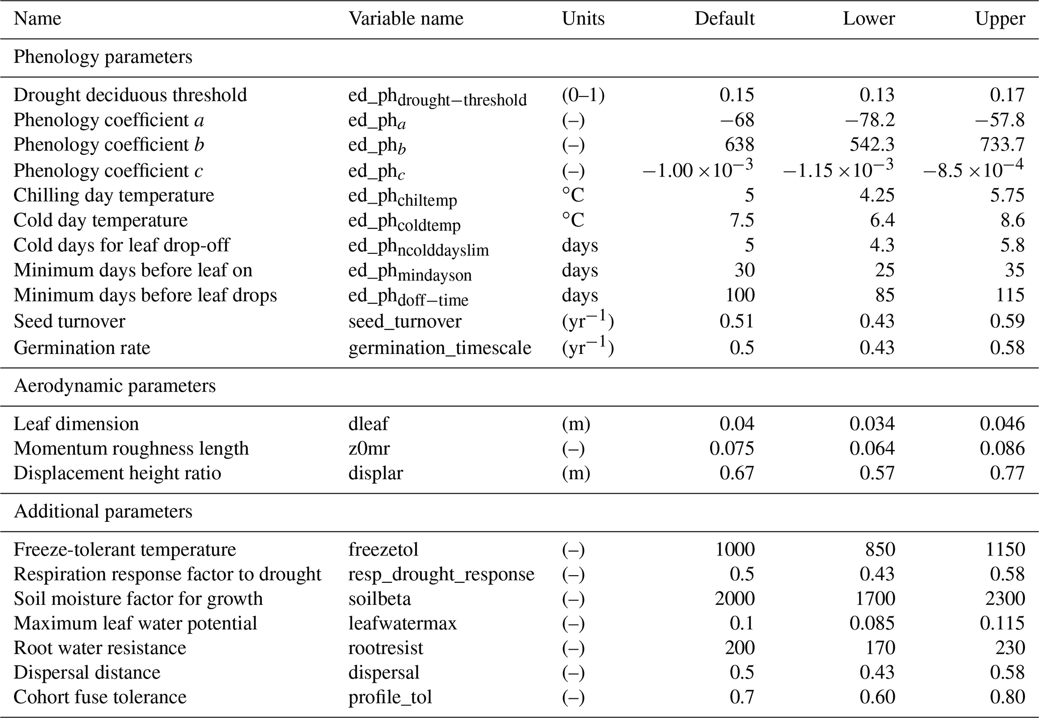
In total, there are more than 200 parameters for all land surface processes including surface energy exchange, hydrology, biogeochemistry, plant physiology, and demographic processes within CLM4.5(FATES). In this study, we focus solely on vegetation components and select 87 parameters that are relevant to vegetation processes, including parameters for photosynthetic processes, temperature response, allometry description, radiative transfer, recruitment, turnover, and mortality. See Tables D1–D4 in the Appendix for a complete list of the parameters used in this study, with corresponding description, units, default values, and applied ranges. Refer to Appendix A for the allometry equations, Appendix B for the temperature response curve (photosynthesis) equations, and Appendix C for the carbon storage equations used in CLM4.5(FATES).
To conduct the sensitivity analysis, we have extracted many parameters in the model that were “hard-wired” in CLM4.5(FATES). The FAST algorithm requires valid ranges to be chosen for each parameter, which creates the possible parameter space to sample from. In theory, each parameter has a corresponding observational distribution that produces the ideal space for sampling (LeBauer et al., 2013). However, in this study, there are both a large parameter set and a scarcity of appropriate data sources for Amazonian forests for many of the relevant quantities; therefore, obtaining a robust data-supported distribution for each parameter was difficult. Because we only aim to understand the baseline model structure, the parameter ranges in this study were generated by applying a uniform distribution over a range that spans ±15 % of the default parameter values of CLM4.5(FATES) (i.e., default parameter values for tropical evergreen trees). We choose a rather conservative range of ±15 % of the default CLM4.5(FATES) values so that global sensitivity indices can be estimated in the reasonable vicinity of the default parameters. We suggest that a more robust uncertainty analysis based on realistic parameter ranges is needed for guidance on additional field measurements.

Figure 2Simulated temporal dynamics in diameter at breast height (dDBH; cm yr−1 tree−1) and the corresponding first-order parametric sensitivity indices. The left panels show the simulated ranges of dDBH for (a) all, (b) small (diameter <10 cm), (c) medium (10 cm < diameter <50 cm), and (d) large trees (diameter >50 cm). Shown is the mean simulation (black line) with 95 % spread of the simulation ensemble. Right panels show the sensitivity for the top six most important parameters for (e) density of all trees, (f) small tree density, (g) medium tree density, and (h) large tree density, in order of importance based on the mean parametric sensitivity across years (red is the most important and blue is the least important). The jumps seen in 10, 40, 70, and 100 years for small, medium, and large trees are due to the temporal averaging mentioned in the materials and methods section. The figures also show sensitivities of the remaining parameters in light grey (first-order sensitivity index for all other parameters) as well as the sensitivity of parameter interactions in dark grey (higher-order sensitivity index for all parameters).
Using FAST, 5000 parameter combinations are sampled from the parameter space. The sample size was determined using the heuristic method of Xu and Gertner (2011a), where it is appropriate to use 100 times the number of effective (important) parameters. The 5000 model runs cost about 32 CPU hours for each simulation, and thus we ran our simulations for a total of 160 000 CPU hours on the Los Alamos National Laboratory (LANL) Conejo supercomputer.
In this analysis, we assume the majority of CLM4.5(FATES) parameters to be non-correlated with uniform probability because our study is focused on the model parametric sensitivity for model behaviors and there is a limitation of data for estimating covariance among the 80+ parameters. However, we do need to take care of the correlation among parameters in the temperature response functions (Appendix B) in order to generate realistic temperature response curves. These parameters are tested for correlation using a published dataset (Leuning, 2002), which showed that the photosynthetic parameters for activation energy (e.g., ) are not necessarily correlated with the other photosynthetic parameters. However, the parameters for deactivation energy (e.g., ) and those related to entropy terms (e.g., ) are highly correlated, as expected (correlation of 0.99+). Thus, each of these parameters' samples are generated from the same location in their relative parameter spaces, which maintains their correlation.
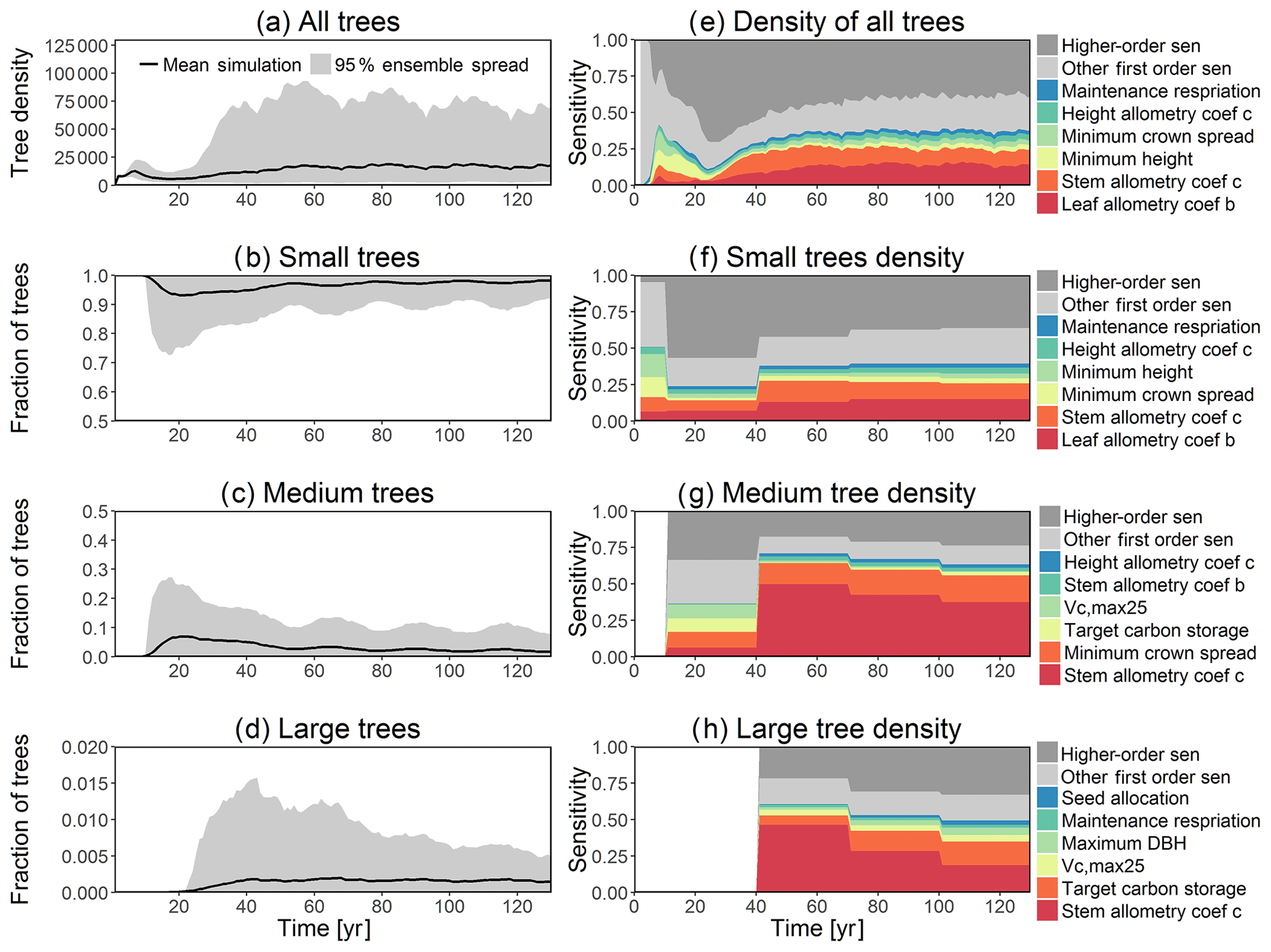
Figure 3Simulated temporal dynamics in tree density (NPLANT; N ha−1) and the corresponding first-order parametric sensitivity indices. The left panels show the simulated ranges of tree density for all trees (a) and the corresponding fraction of (b) small (diameter <10 cm), (c) medium (10 cm < diameter <50 cm), and (d) large trees (diameter >50 cm). Right panels show the sensitivity for the top six most important parameters for (e) all, (f) small, (g) medium, and (h) large trees, in order of importance. See Fig. 2 for details on legends.
2.4 Data and model setup
In this study, the CLM4.5(FATES) model simulations are set up for a 1∘ by 1∘ grid in a moist-tropical forest in the state of Pará, the Amazon, Brazil (7∘ S, 55∘ W), which is a default tropical setup for CLM. The climate conditions for this site are from Qian et al. (2006), representative of data from 1948 to 1972 and recycled for the 130-year simulations (Fig. 1). The CO2 concentration is set as 284.7 ppm. No nitrogen deposition is simulated, as FATES currently does not have the nutrient limitation yet. We initialized the runs with a near-bare ground or a state with no vegetation but available seeds, and simulated the forest dynamics for 130 years, which we determined was enough time for the ecosystem to reach equilibrium because simulated outputs and corresponding sensitivity values for biomass, basal area, and various carbon fluxes had stabilized by this time. By choosing to start from near-bare ground and running the model until it reaches a quasi-steady-state size distribution, rather than by examining short runs initialized from observed initial forest size distributions (e.g., Dietze et al., 2014), we are deliberately allowing the ecosystem demographic structure itself to be an outcome of the parametric variance rather than a separate, possibly non-self-consistent, initial condition variance. The fire component is turned off in view that the study site has limited fire disturbances.
In this section, we highlight the outputs of CLM4.5(FATES) from the 5000 simulations obtained for the FAST analysis and then show the important parameters that control variance in the outputs. We first investigate the forest demographic dynamics, diagnosing the growth and mortality processes simulated in CLM4.5(FATES), i.e., outputs representing the change in diameter at breast height (dDBH), the mortality rate, and the resulting basal area (BA). Then, we analyze the carbon fluxes and stocks in the model simulations including gross primary production (GPP), net primary production (NPP), LAI, and total forest biomass.
3.1 Forest demographic dynamics: growth and mortality
One of the key properties of CLM4.5(FATES) is that vegetation is represented as cohorts of varying sizes for more realistic simulation of light competition in the canopy. To illustrate how different parameters impact different size classes of trees, we group various cohorts of trees into three size classes for analysis purposes: small, medium, and large trees. Since the model runs are initialized from a near-bare-ground state, all simulated plants are considered “small” with an initial density of half-centimeter diameter saplings.
For the stem growth (dDBH averaged per tree; Fig. 2a–d), small trees have lower rates of growth compared to medium or large trees as they are mostly in the understory and thus have a lack of light for photosynthesis. However, the fraction of overall stem diameter growth is dominated by the small trees (Fig. D2) due to their high densities (Fig. 3b). The trees grow faster at the beginning of the simulation when the canopy has not reached full closure. Correspondingly, the parametric sensitivities tends to vary at the beginning of the simulation and then become stable through time. The most sensitive parameters for tree growth are the target storage carbon and stem allometry parameters; however, the importance magnitude varies with time and sizes of trees (Fig. 2e–h). The stem allometry is the most sensitive parameter at the beginning of simulation (<20 years), but the target carbon storage parameter becomes dominant after simulation year 70 (Fig. 2a). We observe that the stem allometry coefficient c is the dominant parameter that controls dDBH for medium and large trees, and the target carbon storage is the most important parameter for small trees. A higher value of stem allometry coefficient c, or a higher allocation of carbon to stem, will lead to a faster growth of diameter at breast height (DBH) in the initial life stage of small trees (Fig. D3a). However, for medium and large trees, a higher allocation of carbon to stem can lead to lower proportion of carbon allocated to leaves for productivity and thus a slower DBH growth (Fig. D3b, c). This outcome supports hypothesis H2, which states the importance of allometric parameters. The target carbon storage determines the target amount of carbon for the plant to store relative to the leaf biomass (see Appendix C for details). Smaller trees have less stem biomass and are less impacted by the stem allometry coefficient c parameter. Furthermore, small trees are vulnerable to changes in the amount of target carbon storage which affects carbon allocation to growth (see Eq. C3 in Appendix C). Our sensitivity analysis also shows specifically important parameters for different sizes of trees. For example, leaf allometry is important for small trees, Vc,max25 for medium trees, and seed allocation for large trees.
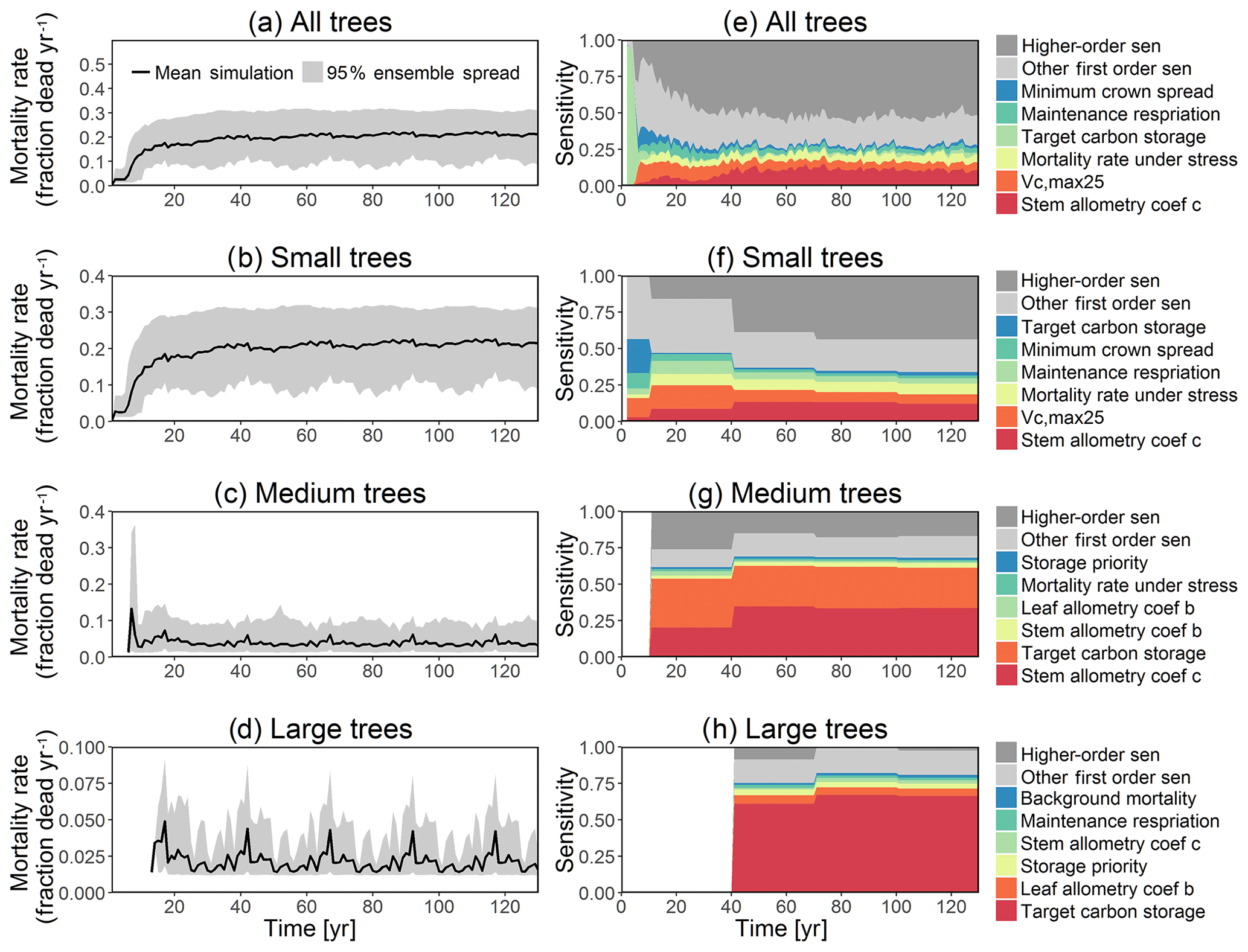
Figure 4Simulated temporal dynamics in tree mortality rates (fraction yr−1) and the corresponding first-order parametric sensitivity indices. The left panels show the mortality rate for (a) all, (b) small (diameter <10 cm), (c) medium (10 cm < diameter <50 cm), and (d) large trees (diameter >50 cm). Right panels show the sensitivity for the top six most important parameters for (e) all, (f) small, (g) medium, and (h) large trees, in order of importance. See Fig. 2 for details on legends.
In this analysis, carbon starvation emerged as the main driver for tree mortality (Fig. D4). The carbon-starvation-based mortality uses a threshold of carbon storage to trigger mortality (see Appendix C). Under shaded conditions, lower carbon stores caused by the balance of NPP, respiration, and tissue growth/maintenance should lead to a higher mortality rate. As expected, the smaller tree size classes have much higher mortality rates (Fig. 4b–d). The first-order sensitivity analysis of predicted mortality rate (percentage of mortality per year) shows that the dominant parameter for predicting mortality of large trees is the target carbon storage (Fig. 4h); however, for small and medium trees, other parameters such as allometric and photosynthetic parameters that could potentially determine their height growth and competitive advantages in the canopy are also important (Fig. 4f, g). Specifically, for medium-sized trees, the mortality rate is affected by both the stem allometry coefficient c and targeted carbon storage (Fig. 4g). For the small trees, important parameters include the photosynthetic capacity parameter (Vc,max25), stem allometry coefficient c, mortality rate under stress, and maintenance respiration, with the target carbon storage having high sensitivity for small trees in the early years (Fig. 4f).
The simulated basal area (BA) of the forest, which is the total stem cross-sectional area per ground surface area, results from the combination of both DBH growth and mortality. The BA reaches equilibrium for different sizes of trees around year 70 (Fig. 5a). Our FAST analysis shows that a key parameter that controls BA in different tree size classes is the stem allometry coefficient c (Fig. 5e–h), which is a major parameter that determines the DBH growth (Fig. 2). We also found that the target carbon storage parameter that dominantly controls mortality is an important parameter for the simulated BA (Fig. 5e–h). Different from parameters important for DBH growth at the individual tree level and mortality rate, a new parameter that becomes important for BA of small and medium trees is the minimum crown spread, which determines the ratio of crown radius to DBH. A larger crown spread can lead to a smaller number of trees in the canopy and thus a lower BA (Fig. D5). The identified important parameters for the simulated tree density and fraction of trees are very similar to those identified for the simulated BA, except that the leaf allometry coefficient b becomes very important for simulated small tree densities (Fig. 3e–h) and minimum height for fraction of trees (Fig. D6).
For the second-order sensitivity analysis, parametric interactions between stem allometry coefficient c and the proportion of carbon for seed allocation, and target carbon storage are found to be important for the prediction of total BA (Fig. D7). For trees of different sizes, parametric interactions between stem allometry coefficient c and minimum crown spread, target carbon storage, and maximum DBH are important for small, medium, and large trees, respectively. For the prediction of dDBH and mortality, the contributions of most parametric interactions are relatively small except for large trees (Fig. D8). The interactions between stem allometry coefficient c and the proportion of carbon for seed allocation, maximum DBH, and stem allometry coefficient b are important for the prediction of dDBH for large trees. With respect to large tree mortality, the interaction between stem allometry coefficient c and target carbon storage is found to be important (Fig. D9).
3.2 Forest carbon cycles: carbon fluxes and stocks
To investigate the key parametric control on carbon fluxes and stocks, we specifically investigate parameter sensitivities for GPP, NPP, LAI, and total forest biomass. Our results show that GPP and NPP increased consistently for the first 10 years of the simulations, which is expected for a forest growing from bare ground (Fig. 6). However, within a fairly short period of 5–10 years, GPP, NPP, and LAI and their variance reached a quasi-stable rate. This amount of time to reach equilibrium is much shorter compared to the basal area (Fig. 6a) and the total biomass accumulations (Fig. 6d).
The first-order sensitivity analysis based on FAST shows that, for carbon fluxes of GPP and NPP, the photosynthetic capacity parameter (Vc,max25) is the most sensitive parameter (Fig. 6e, f), which supports hypothesis H1. Furthermore, specifically for NPP, the respiration parameters such as the growth respiration fraction and leaf maintenance respiration rate show high sensitivity (Fig. 6f). For LAI, the leaf allometry coefficient b is the most important, as it determines carbon allocation for leaves (Fig. 6g). The stem allometry coefficient c is the most important for total biomass (Fig. 6h), as it determines carbon allocation to the stem, which supports hypothesis H2. See Fig. D10 for an easier comparison of parametric sensitivities for different model outputs. A common sensitive parameter is the target carbon storage, which is important for GPP, NPP, LAI, and total biomass. This results from the fact that the target carbon storage is a key driver for mortality especially for medium and large trees in the simulations (Fig. 4e–h), which account for a large proportion of total biomass (Fig. D11) and GPP (Fig. D12). This result supports hypothesis H3. For the second-order sensitivity, the contributions of most parametric interactions are relatively small (Fig. D13), as the first-order sensitivity accounts for a majority of the total variance in model outputs (Fig. 6e–h).
To understand how climate will impact sensitivity results, we also calculated the Spearman rank correlation coefficients between the first-order sensitivity index and the corresponding climate drivers. Our results show that the sensitivity of target carbon storage and maintenance respiration rate is negatively correlated with annual mean precipitation and relative humidity but is positively correlated with annual mean air temperature. This suggests that they are more important during the period of stressed conditions comprised of low precipitation, low humidity, and high temperature (Fig. 7). Sensitivity to the leaf allometry coefficient b is positively correlated with annual mean precipitation and relative humidity. This suggests the leaf carbon allocation is more important under favorable environmental conditions for growth. In general, our results suggests the climate has a larger impact on the parametric sensitivities for short-term carbon fluxes (GPP and NPP) and vegetation status (LAI) but has a smaller impact on parametric sensitivities for long-term vegetation carbon stocks.
Our bivariate spline analysis (Wahba, 1990) shows that, for Vc,max25 and target storage carbon, an increase in either of these parameters will cause an increase in the output of GPP, NPP, LAI, and biomass (Fig. 8). For the parameters related to leaf and stem allometry, however, the relations may differ depending on the output and the year of interest. At year 130, the higher leaf allocation normally leads to higher fluxes (NPP and GPP) but less biomass. Meanwhile, higher stem allocation leads to higher biomass but smaller fluxes (NPP and GPP). This suggests that the trade-offs between carbon allocation to stem vs. leaf tissues leads to a corresponding trade-off between carbon stocks and productivity in the model predictions.
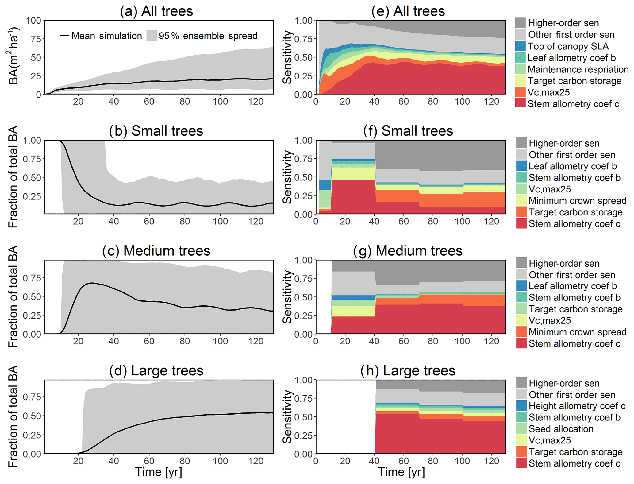
Figure 5Simulated temporal dynamics in basal area (BA, m2 ha−1) and the corresponding first-order parametric sensitivity indices. The left panels show the simulated ranges of BA for (a) all, (b) small (diameter <10 cm), (c) medium (10 cm < diameter <50 cm), and (d) large trees (diameter >50 cm). Right panels show the sensitivity for the top six most important parameters for (e) all, (f) small, (g) medium, and (h) large trees, in order of importance. See Fig. 2 for details on legends.
4.1 Comparing parameter sensitivities to other models
While second-generation vegetation demographic models such as CLM4.5(FATES) provide new opportunities to predict the global carbon cycle, the larger number of parameters also creates challenges for identifying key processes for further investigation. In this study, we apply a global sensitivity analysis to determine the influential parameters over a specified region of the parameter space. So far, several uncertainty and sensitivity analyses have been conducted for size-structured land surface models (Pappas et al., 2013; LeBauer et al., 2013; Wang et al., 2013; Dietze et al., 2014; Collalti et al., 2019). In comparison with previous sensitivity analyses of size-structured models, our study considers a much larger number of parameters, i.e., >80 compared with ∼20–35 parameters (Pappas et al., 2013; LeBauer et al., 2013; Wang et al., 2013; Dietze et al., 2014), the difference in parametric sensitivity for different tree sizes, and the interactions among the key parameters. In general, our analysis shows similar results to sensitivity analysis on first-generation “big-leaf” vegetation models (e.g., Sargsyan et al., 2014), which show the importance of photosynthetic capacity, Vc,max25, for predicting GPP and NPP. However, we do show important parameters that are unique to LSMs with second-generation vegetation demography. Specifically, results shown here indicate the importance of leaf and stem allometry parameters, which control dynamic carbon allocation strategies based on size, and thus control the general vegetative state and size structure of the forest (Waring et al., 1998; Waring and Running, 2010). Importantly, a significant amount of variability in allometry is reported for different species and regions of the world (Feldpausch et al., 2011; Dietze et al., 2008), and thus it is critical to achieve an accurate parameterization of allometry for second-generation vegetation demographic models within LSMs. The importance of allometric parameters could result from the fact that the relationship between allometric coefficients and carbon allocation is highly nonlinear based on a power function (see Appendix A for details). This result is in agreement with the results from a recent sensitivity analysis study using a size-structured vegetation model (Collalti et al., 2019). Our sensitivity analysis also shows the importance of carbon storage for the prediction of mortality rate and thus the total biomass. This is in agreement with other sensitivity analyses of CLM which show the plant mortality rate as a key parameter for the prediction of total biomass (Sargsyan et al., 2014). However, we do want to point out that there could be a potential bias as carbon starvation is the main mechanism that kills trees in the simulations in our study; however, in reality, there could be many other causes of mortality such as wind, insects, and fire (see McDowell et al., 2018 for a review). The current implementation of hydraulic failure in CLM4.5(FATES) is only based on very low soil moisture thresholds and more mechanistic representation of plant hydrodynamics (e.g., Christoffersen et al., 2016) could result in the importance of hydraulic traits for mortality and vegetation dynamics. By exploring parametric sensitivity for small, medium, and large trees, we show that the ranking of parameter importance changes with the size of plants (e.g., Fig. 2). This result is in agreement with a recent study that showed the influence of certain functional traits varied with size (Falster et al., 2018).
In our analysis, we observed a number of key similarities in model response to parameter variations in photosynthetic capacity, mortality, and respiration parameters (Pappas et al., 2013; LeBauer et al., 2013; Wang et al., 2013; Dietze et al., 2014); however, there are differences in the order of parameter importance. For example, Dietze et al. (2014) showed that growth respiration fraction was the most important parameter for the simulation of NPP, and Vc,max25 only ranked as the seventh most important parameter. For our analysis, Vc,max25 and growth respiration fraction are the first and second most important parameters. This difference in parameter sensitivity rank may result from the fact that Dietze et al. (2014) used variable parameter ranges based on data (i.e., an uncertainty quantification study), while our sensitivity analysis uses equal percentage variations (see details in the discussion “limitation of methods” subsection). We also found that some parameters that are identified as important in other studies are not found to be important in our analysis. For example, Dietze et al. (2014) showed that water conductance that determines the upper boundary of transpiration is the second most important parameter for simulated NPP, but a similar parameter (smpso; Table D2) that defines soil water potential for opening stomata is not important in our analysis. This could be related to the fact that our site is much wetter than the temperate forests simulated by Dietze et al. (2014). Pappas et al. (2013) showed that the root distribution parameter that determines the fraction of fine roots in the upper soil layer is one of the top five parameters for the simulations of vegetation carbon fluxes and stocks; however, in our sensitivity analysis, the two root distribution parameters (roota and rootb; Table D2) are not important for both vegetation carbon fluxes and stocks. This difference could also result from a wider range of variations ( %) in the study of Pappas et al. (2013) compared to our 15 % variations of the default parameters. Finally, our analysis shows the importance of allometry parameters, which are not considered in many previous studies (Pappas et al., 2013; LeBauer et al., 2013; Wang et al., 2013; Dietze et al., 2014).
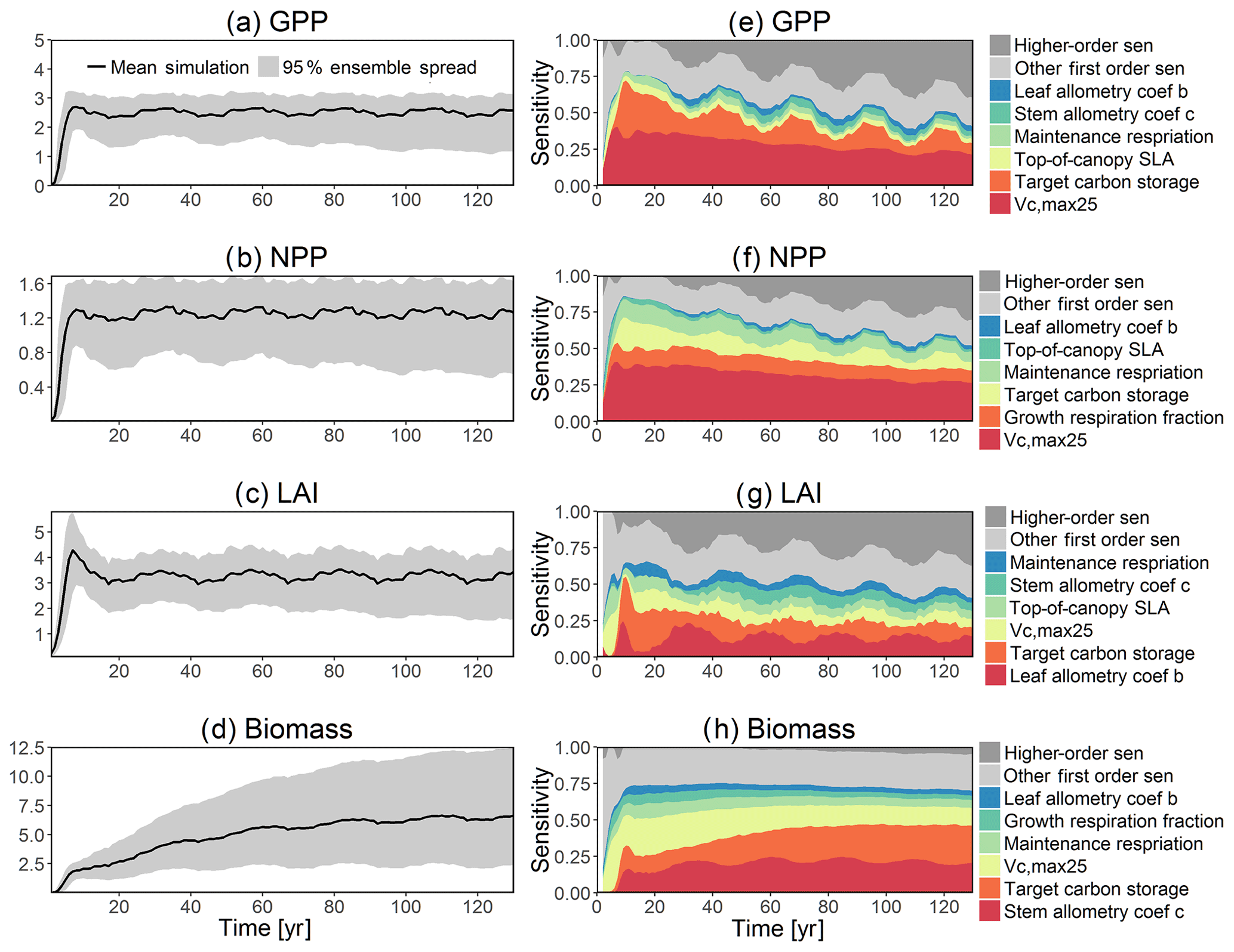
Figure 6Simulated temporal dynamics in carbon fluxes and stocks, and the corresponding first-order parametric sensitivity indices. The left panels show the simulated ranges for (a) GPP (kg C m−2 yr−1), (b) NPP (kg C m−2 yr−1), (c) LAI (m2 m−2), and (d) total biomass (kg C m−2). Right panels show the sensitivity for the top six most important parameters for (e) all, (f) small, (g) medium, and (h) large trees, in order of importance. See Fig. 2 for details on legends.
4.2 Comparing simulations with observations
The goal of our study is not to reproduce the observations but instead to identify important parameters that can be better estimated for the model to fit observations. Thus, we lay out potential parameter estimation improvements to achieve this goal. We do want to highlight three caveats. First, improved estimation of the most sensitive parameters may not be most efficient if they have relatively small uncertainty or variability across different species and locations. Second, even if the estimates for most sensitive parameters are perfect, we may still not be able to fit model predictions to observations if there is deficiency in the representation of key processes in the model. Third, the recycled climate drivers from 1948 to 1972 may not match the observational periods. Given observation data limitations for our site, we conduct a qualitative comparison of our model simulations to ranges reported in the literature for the tropics. Not surprisingly, our model results show a variation of model–data mismatch for key vegetation states. For LAI (Fig. 6c), our simulated range is between ∼1.9 and 6.0 m2 m−2, which is lower than the observed range of ∼3.0–6.9 m2 m−2 based on LAI estimated from MODIS (Knyazikhin et al., 1999) during 2000–2016 within a 0.5∘ window around our site. Our sensitivity analysis showed that leaf allometry coefficient b and target carbon storage are two key parameters for simulated LAI (Fig. 6g), and we expect that a better estimation of these parameters with data could potentially improve the model simulations. For GPP (Fig. 6a), the simulated range is between ∼1.0 and 3.0 kg C m−2 yr−1, which is also lower than the observed range of ∼2.4–3.7 kg C m−2 yr−1 based on extrapolation from eddy flux tower observations and climate during 1981–2010 (Jung et al., 2009). Our analysis suggests that photosynthetic capacity, as represented by Vc,max25, target carbon storage, and top-of-canopy specific leaf area, is an important parameter (Fig. 6a), and an improved estimation of them could help improve model simulations of GPP. We are not able to access on-site data for other model outputs. Therefore, we compare our model outputs with ranges from multiple tropical sites to evaluate their validity. For biomass (Fig. 6d), the simulated range of ∼2.5–12.5 kg C m−2 is lower than the observed range of ∼7.3–21.3 kg C m−2 from 21 transects within three tropical sites (Hunter et al., 2013). For BA (Fig. 5a), the simulated range of ∼5.0–30.0 m2 ha−1 is also lower than the observed range of ∼17.1–35.2 m2 ha−1 from five tropical sites (Hunter et al., 2013). Our results show that stem allometry coefficient c is the most important control on BA and biomass, and an improved parameterization on stem allometry could help improve the model simulations. For the DBH growth, there are large variances in the observed values across different sites with the range of 0–3 cm yr−1 (Lieberman et al., 1985; Worbes, 1999; Adams et al., 2014). The simulated average DBH growth is between 0 and 0.4 cm yr−1 but could be as high as 4 cm yr−1 for medium and large trees (Fig. 2). Based on our sensitivity analysis (Fig. 2), we expected an improved parameterization of both allometry coefficient c and target carbon storage could help fit the model predictions to data.
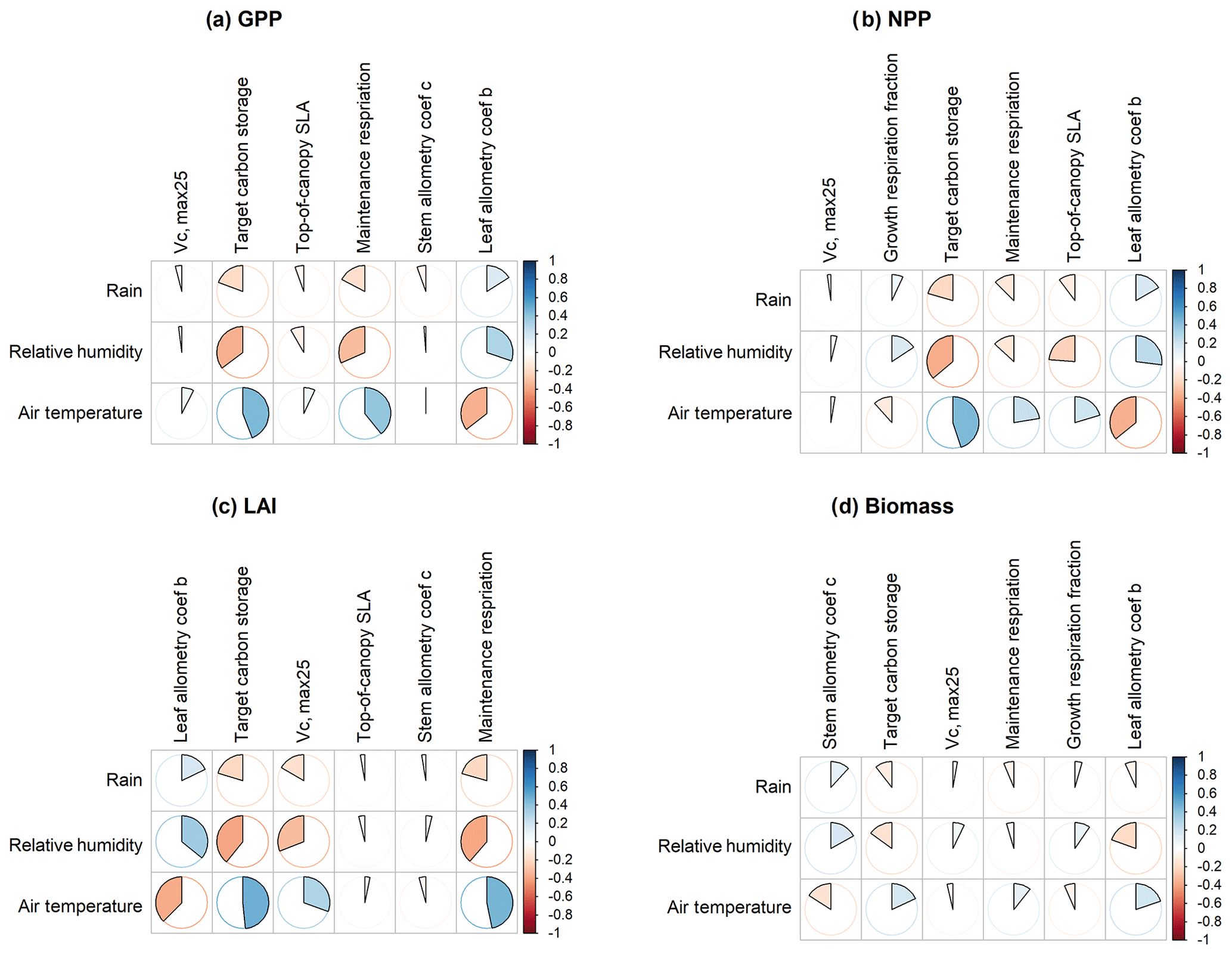
Figure 7Spearman's correlation coefficients between climate drivers and six most important parameters identified for (a) GPP, (b) NPP, (c) LAI, and (d) biomass.
We compare our mortality simulations with an extensive dataset of observed mortality of 1781 species from 14 pan-tropical large-area ForestGEO forest dynamics plots (Johnson et al., 2018). For this study, the forest plots ranged from 2 to 52 ha each, with 371 ha in total, in which all recorded stems are ≥1 cm diameter at breast height. Our comparison shows that the CLM4.5(FATES) simulations of medium and large tree mortality (Fig. 4c, d) are close to the 95 % confidence interval of observed values, which is about ∼0.5 %–5.7 % per year. However, for small and medium trees (Fig. 4b, c), the simulated mortality rate of ∼15 %–30 % and ∼1 %–10 % is high when compared to the observed 95 % confidence interval of mortality rate of ∼0.6 %–11.3 % and ∼0.8 %–3.0 % for small and medium trees, respectively. The high predicted mortality rate of small trees could result from the fact that the model predicts a very high mortality rate for very small trees (<1 cm), as they cannot survive after establishment due to low light conditions in the simulations. Since the small trees have such a large fraction of the population in our simulations (Fig. 3b), the overall mortality rate (Fig. 4a) of ∼15 %–30 % is also high when compared to observations (∼0.6 %–11.3 %); however, if we separate the mortality rate of very small trees from the calculation of the overall mortality, then the simulated mortality rates of 1 %–10 % (Fig. D14b) are in the range of observations. The very high mortality rate range of smaller trees (∼10 %–30 %; Fig. D14a) spans the reported seedling/sapling mortality rate, e.g., ∼15 %–21 % per year from 1- to 20-year-old tropical forest stands in Costa Rica (Dupuy and Chazdon, 2006). However, there is potential for improvement for site-level simulations as the current recruitment algorithm within CLM4.5(FATES) depends only on the availability of seed bank but not on the density, light, and water availability. The relatively high mortality rate of small and medium trees could also be linked to the fact that CLM4.5(FATES) uses the perfect plasticity approximation (PPA) to simulate the canopy light availability for understory trees (Fisher et al., 2018), which may create canopy closure too fast for the small- and medium-sized trees to survive under low light conditions. We expect that future improvements in recruitment and representation of the light environment within the PPA could be helpful for a better prediction of tree mortality for small- and medium-sized trees. It is also possible that the observed mortality rate for small trees could potentially be underestimated if all the trees in a certain size classes died at a shorter time frame than the census intervals. Our sensitivity analysis indicates that key model parameters that can be better estimated for improved mortality predictions include stem allometry parameters, Vc,max25, target carbon storage, and mortality rate under stress (Fig. 4).
Another reason for the data–model discrepancy could result from the limited representation of diverse tropical species or traits with the simulation of a single PFT. This is a limitation of many LSMs, as they typically only have two to three PFTs for tropical forests (e.g., only evergreen and deciduous for tropical trees within CLM). CLM4.5(FATES) has the potential to better represent the trait diversity through trait filtering under different environmental conditions (Fisher et al., 2010, 2015). One critical component to incorporate traits into the model is to represent the trait trade-off and coordination for different PFTs. Through our sensitivity analysis, we have identified key parameters for vegetation dynamics, which can be targeted for the representation of trait trade-off and coordination in the tropics. For example, our study shows that a higher stem carbon allocation could reduce the GPP and a higher Vc,max25 could increase GPP (Fig. 8). The potential exploration of trade-off and coordination between these two parameters could be critical to resolve different PFTs and represent the trait variations. Even though the simulated ranges of the model outputs are different than the observations, our sensitivity analysis should still be valid in view that a primary end goal of this research is to identify important parameters that can be better estimated for the model to better fit observations. For example, Holm et al. (2019) utilized results from our study to implement their tropical forest parameterization, specifically by increasing their target carbon storage parameter to obtain higher survival and lower growth.
In addition to directly comparing the model outputs to observations, we want to highlight that the sensitivity analysis will also allow us to explore the functional relationships between model parameters and outputs. Future synthesis studies that show these functional relationships using data across different sites could be very useful to evaluate the fidelity of model structure to represent the key processes that control these relationships.

Figure 8Relations between outputs of CLM4.5(FATES), including GPP, NPP, LAI, and biomass (units shown in Fig. 6), and the most sensitive parameters, i.e., Vc,max25 (units are ), target storage carbon (unit is the ratio of leaf biomass), leaf and stem allocation (unitless parameters) for simulation year 10 (red) and 130 (blue). Shown are the mean relations with the 95 % confidence intervals in grey envelopes. These figures show how an output will generally increase or decrease when a given parameter is changed.
4.3 Limitation of methods
Our study is the first global sensitivity analysis for CLM4.5(FATES); however, it is subjected to several limitations that could be improved for future studies. First, our study uses an arbitrary choice of parameter ranges (±15 %), which determines the variance in the model outputs and the corresponding results of the sensitivity analysis. However, we expect that our analysis can reveal the importance of parameters given equal percentage of variations, which can help us gain a better understanding of the model structure. We do acknowledge that uncertainty analysis studies that specifically consider the potential ranges of values in tropical forests based on observations could provide insights on which additional measurements are needed to explain variance in the model prediction.
Second, we only consider the correlation in pairs of parameters that determine temperature responses for deactivation energy and entropy in photosynthesis. We do want to point out that the potential correlation among other parameters (Díaz et al., 2016), such as the trade-off between mortality and growth parameters and the correlation among coefficients for allometric equations, could affect the simulated model output ranges and the sensitivity results. However, our exploration of parameter sensitivity assuming their independence could still help us understand the baseline parameter control on model behaviors (Xu and Gertner, 2009). The exploration of trade-offs and coordination among different parameters requires data analysis for multiple traits of the same species. The Predictive Ecosystem Analyzer (PEcAn) framework (LeBauer et al., 2013) could be a useful tool to synthesize plant trait data to estimate model parameter distributions. The challenge is that, even though there are great efforts in the research community to compile plant trait data across the globe (Kattge et al., 2011a, b), there are still limited datasets with observations of multiple traits for the same species. Future uncertainty analysis studies that explicitly consider the prior distributions and correlations for all the parameters can build on this analysis and gain further insights on where the uncertainty in the model predictions comes from.
Third, it is possible that the parameter sensitivity could be different if we use different model inputs, different sites, and different structures of subcomponents within the model. For example, using site-level climate drivers, instead of the reanalysis meteorological drivers used in this study (Qian et al., 2006), could lead to different sensitivity values since our analysis showed that parameter importance is quite sensitive to different climate conditions. Furthermore, there are ongoing development activities to improve different components of the models. For example, there are current efforts to incorporate different representations of tree allometry within CLM4.5(FATES), which have different formulations between size and biomass, e.g., Chave et al. (2014), or the current formulation of the photosynthetic process in the CLM4.5(FATES) can be replaced with a model that more accurately represents the allocation of nitrogen and thus the photosynthetic process (see Xu et al., 2013; Ali et al., 2016). Therefore, model improvements such as these can affect corresponding sensitivity analysis results. To understand the impact of site-level variations on model dynamics, similar sensitivity analysis across different sites can be conducted to understand how climate variability will affect the sensitivity analysis results.
Finally, although the FAST method presented in this study can provide a comprehensive analysis of the parameters that control vegetation demography, it is mostly built on statistical relationships (e.g., Fig. 8). A complementary approach is to use more tractable theoretical ecology models (e.g., Farrior et al., 2016 and Falster et al., 2018) to approximate the underlying model input–output relationships, which can provide more mechanistic understanding of model behaviors.
LSMs have many parameters that could potentially affect the outcome of their simulations. In this study, we use the FAST analysis to conduct a high-dimensional global sensitivity analysis on CLM4.5(FATES). We use an intermediate complexity of simulation: runs are sufficiently long to permit short-term physiological variance to propagate into the long-term forest demographic structure. Even though we do not explore competitive dynamics between different PFTs, our sensitivity analysis will guide us on the selection of key plant traits for the consideration of trait trade-off and coordination in order to improve PFT coexistence within CLM4.5(FATES).
Our analyses show that the target carbon storage and stem allometry parameters are important for the simulation of DBH growth for individual trees and tree mortality. The photosynthetic parameter,Vc,max25, is the most important for the simulation of carbon fluxes including GPP and NPP. The combination of stem allometry, target carbon storage, and Vc,max25 dominantly control the simulation of total BA and long-term carbon stocks. These identified growth and survival parameters will help us better understand the key control of fast and slow carbon and vegetation dynamics within the next generation of demographically enabled LSMs toward improved model parameterization and model structure.
The results of the sensitivity analysis presented here can be utilized to construct the parameter-output response surface for the CLM4.5(FATES) model, which can assist future efforts for model calibration or diagnosis. These findings may help us better understand the overall model structure and guide the estimation of key model parameters with significant control over vegetative processes in these models for better model fitting to data. The FAST analysis provides a promising means of analyzing complex LSM components and can be a powerful tool in understanding the necessarily high-dimensional representation of living systems within Earth system models.
To access the FATES source code, visit https://github.com/NGEET/fates (last access: 15 May 2018). The FAST methodology described herein is available at https://sites.google.com/site/xuchongang/uasatoolbox (last access: 15 May 2018). The version of the model codes used in this paper and the corresponding model simulations from all 5000 parameter combinations as well as simulation of the default parameter set are available at the NGEE tropics data archive (https://doi.org/10.15486/ngt/1497413, Massoud et al., 2019b) and also upon request from the corresponding authors.
The following equations are cohort-based calculations for allometry in CLM4.5(FATES). Interested readers are referred to Fisher et al. (2015) for more information. The parameters used for the allometry equations include dbh2hm, dbh2hc, dbh2bda, dbh2bdb, dbh2bdc, and dbh2bdd (all are unitless variables). Specifically, the dead wood biomass (BD; kg C) is calculated as a function of diameter (DBH; cm), height (h; meter), and wood density (g cm−3):
The height (m) is calculated based on DBH (cm) as follows:
The parameters used for the temperature response curve equations include the equation to calculate the maximum carboxylation rate, Vc,max25, the maximum electron transport rate, Jmax, and the triose phosphate use (TPU) limited carboxylation rate, TPU (also all parameters here are unitless) (Fisher et al., 2015). The temperature response equations for , Jmax,z, and TPUz are
where tfrz is the freezing point of water in Kelvin (273.15 K).
The target carbon storage is the cushion parameter shown in Table D3. Specifically, a higher value of this parameter will lead to a higher allocation of carbon to storage and thus a lower allocation to growth at the specific time step. Also, carbon storage plays an important role for the simulated mortality through the parameter that controls the mortality rate under stress, stress_mort in Table D3. The tree will be under stress when it has low carbon storage (< leaf biomass). Therefore, the target carbon storage parameter and the mortality rate under stress parameter play a large role in determining the level of mortality that occurs in the simulations.
Carbon storage, bstore (in kg C/cohort), plays a very important role in both growth and mortality (Fisher et al., 2015). Specifically, CLM4.5(FATES) assumes a target carbon storage determined by the multiplication of leaf biomass (bleaf) and the target carbon storage parameter (i.e., the target amount of carbon plants store relative to leaf biomass; Scushion, variable cushion in Table D3). At the specific time, the carbon balance for growth and storage is calculated as follows:
where Tmd is the maintenance respiration and fmd,min is the minimum fraction of the maintenance demand (storage priority parameter in Table D1) that the plant must meet each time step, which represents a life-history-strategy decision concerning whether leaves should remain on in the case of low carbon uptake (a risky strategy) or not be replaced (a conservative strategy).
The fraction of the carbon balance for each cohort allocated to the carbon storage pool (fstore) will be determined by the following equations:
where
Thus, the target carbon storage parameter, Scushion, can affect carbon allocations. Specifically, a higher value of Scushion will lead to a higher allocation of carbon to storage and thus lower allocation to growth at the specific time step.
Carbon storage also plays an important role for the mortality. Specifically, carbon starvation mortality (Mcs) is calculated as follows:
where Sm is the stress mortality factor (i.e., stress_mort in Table D3).

Figure D1Comparison of first-order parametric sensitivity for medium (10 cm < diameter <50 cm) tree density averaged over 20, 30, and 40 years.
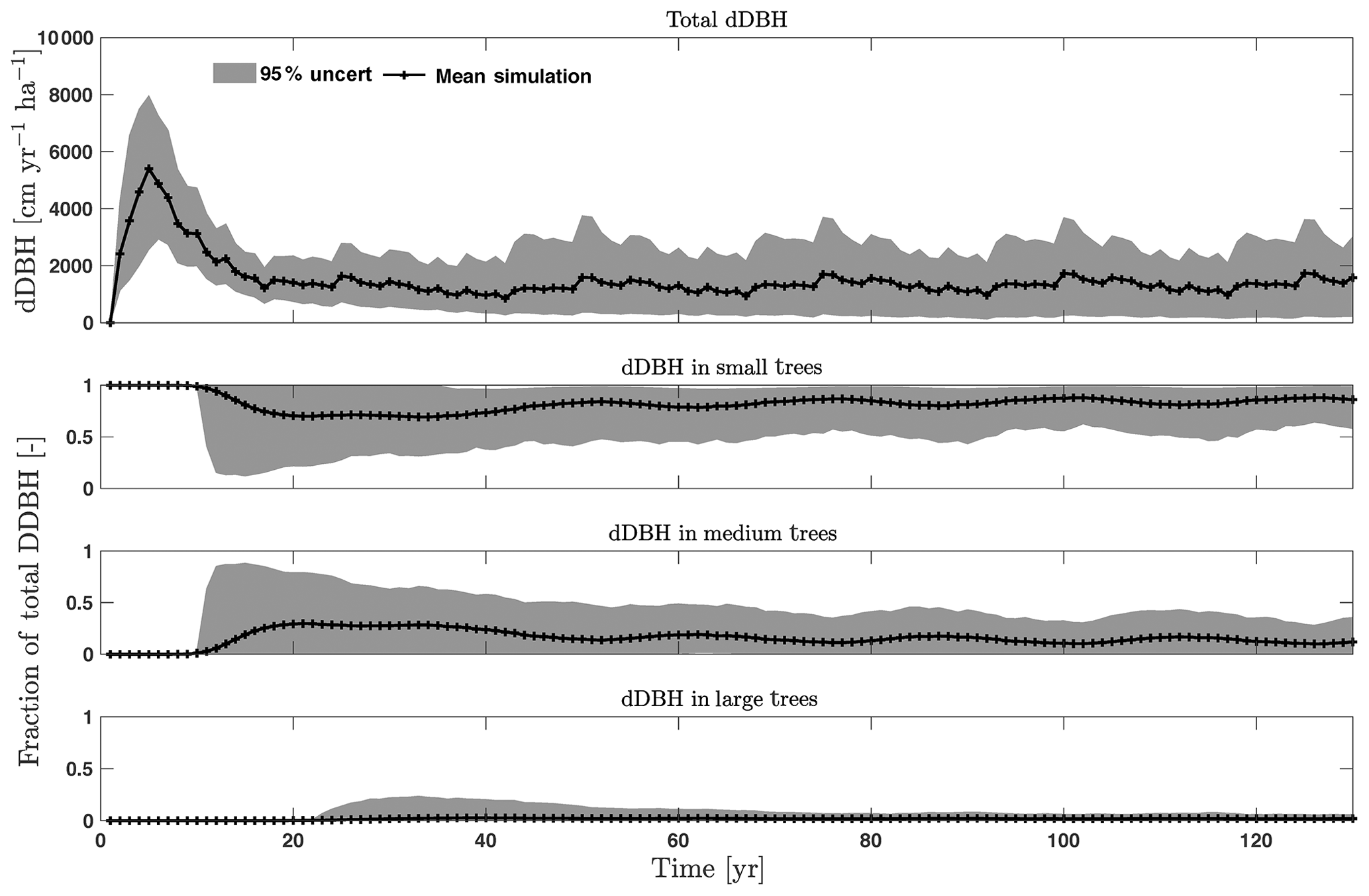
Figure D2Simulated total change in diameter at breast height (dDBH) from CLM4.5(FATES) for all trees and its fractional distribution for small (diameter <10 cm), medium (10 cm < diameter <50 cm), and large trees (diameter >50 cm). Shown is the mean simulation (black line) with 95 % spread of the simulation ensemble.
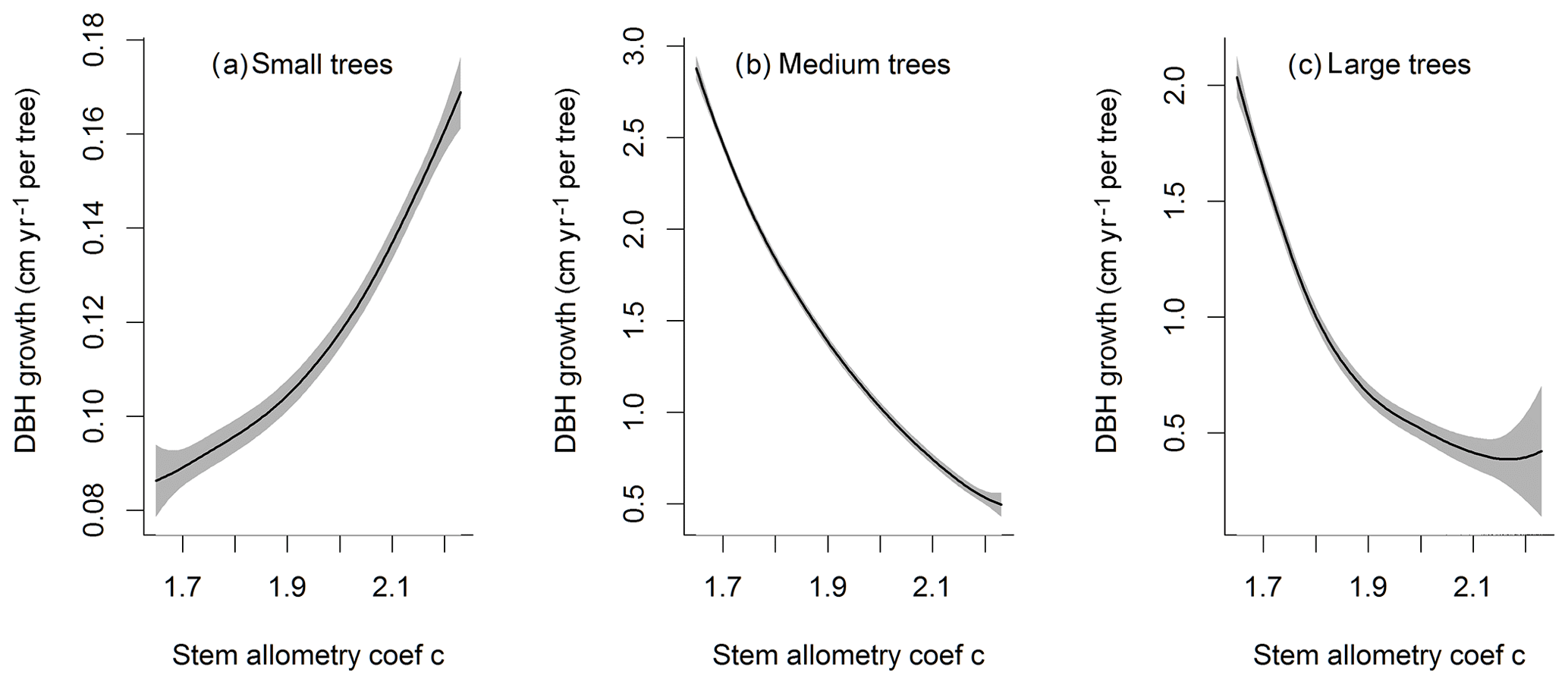
Figure D3Impacts of stem allometry on the change in diameter at breast height (dDBH) averaged over the simulation years 100–130 for trees of different sizes. The shaded area shows the 95 % confidence interval of these relations.
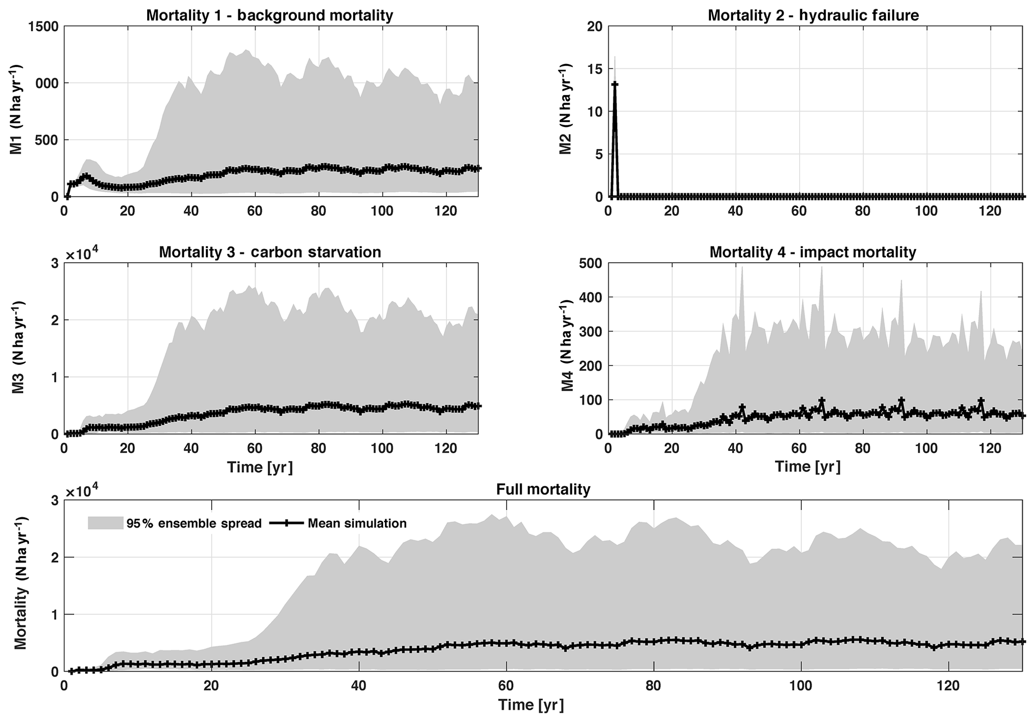
Figure D4Mortality outputs from CLM4.5(FATES), including the mechanisms of M1 – background mortality, M2 – hydraulic failure, M3 – carbon starvation, and M4 – impact mortality. The bottom panel shows the total mortality, which is the sum of M1–M4. Shown is the 95 % (light grey) spread of the simulation ensemble, along with the mean simulation (black lines).
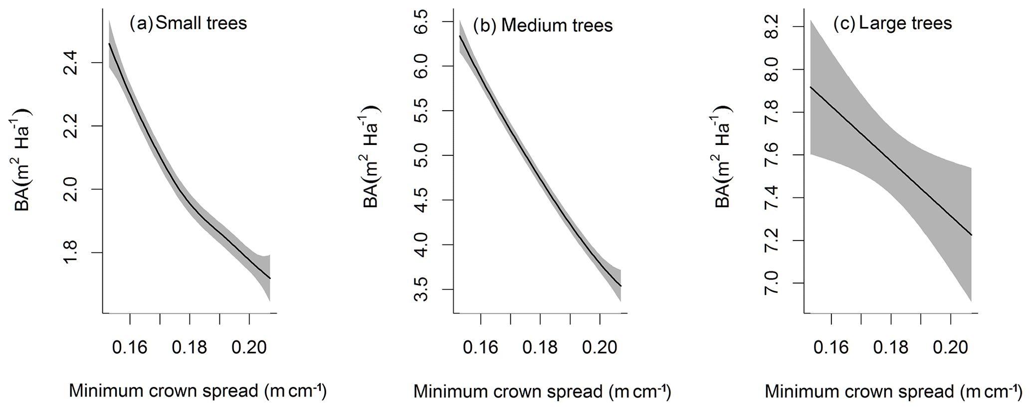
Figure D5Impacts of minimum crown spread on the basal area (BA) averaged over the simulation years 100–130 for trees of different sizes. The shaded area shows the 95 % confidence interval of these relations.
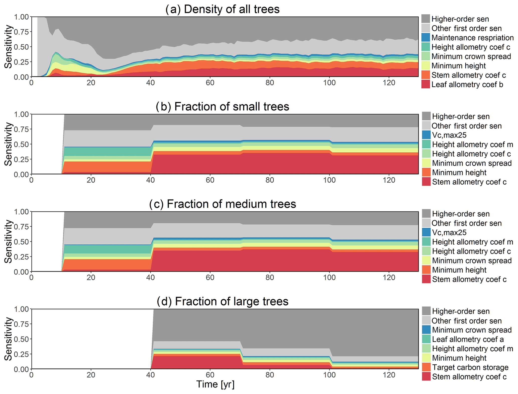
Figure D6First-order parametric sensitivity indices for tree density of all trees (a) and the corresponding fraction of (b) small (diameter <10 cm), (c) medium (10 cm < diameter <50 cm), and (d) large trees (diameter >50 cm). See Fig. 2 for details on legends.

Figure D7Second-order sensitivity index of the model parameters for the basal area (BA) outputs from CLM4.5(FATES) for (a) all trees, (b) small trees, (c) medium trees, and (d) large trees. Shown are the top eight most important parameter interactions in order of importance based on the mean parametric sensitivity across years (red is the most important and blue is the least important)
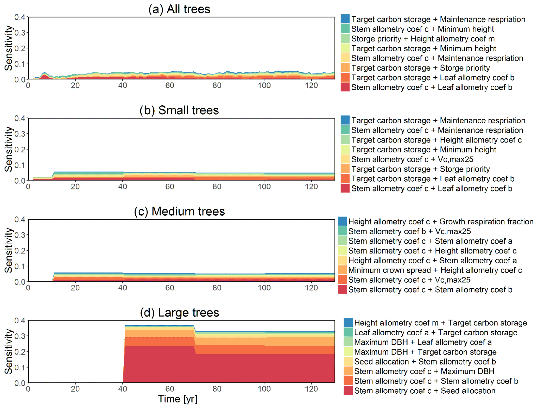
Figure D8Second-order sensitivity index of the model parameters for the change in diameter at breast height (dDBH) outputs from CLM4.5(FATES) for (a) all trees, (b) small trees, (c) medium trees, and (d) large trees. Shown are the top eight most important parameter interactions in order of importance based on the mean parametric sensitivity across years (red is the most important and blue is the least important).
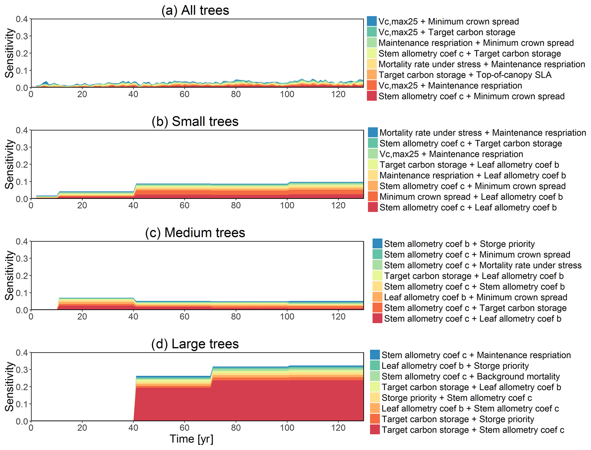
Figure D9Second-order sensitivity index of the model parameters for the mortality outputs from CLM4.5(FATES) for (a) all trees, (b) small trees, (c) medium trees, and (d) large trees. Shown are the top eight most important parameter interactions in order of importance based on the mean parametric sensitivity across years (red is the most important and blue is the least important).
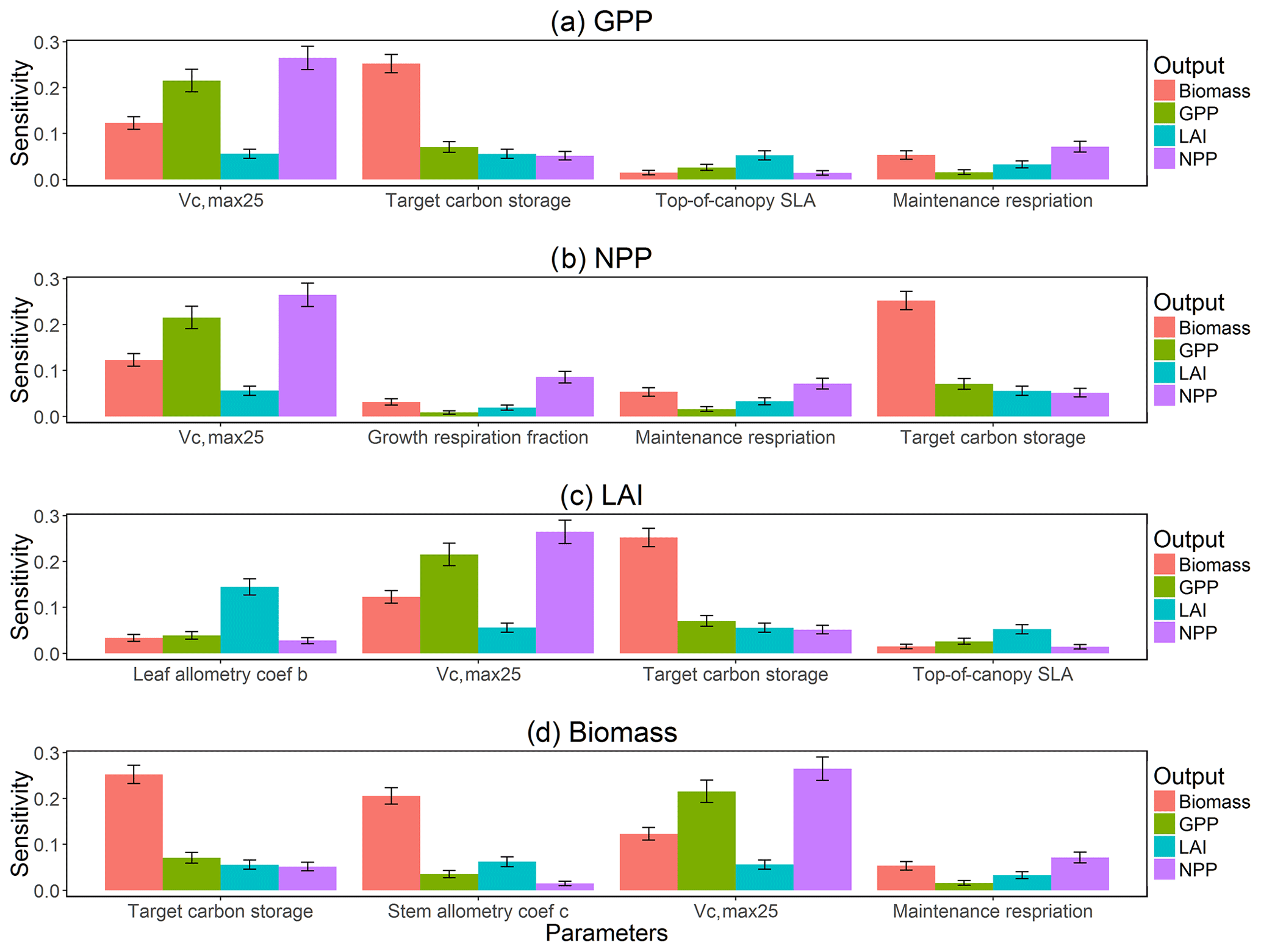
Figure D10Comparisons of parametric sensitivities and the corresponding 95 % confidence intervals for different model outputs at year 130. Shown are the identified four most important parameters for (a) GPP, (b) NPP, (c) LAI, and (d) total biomass.
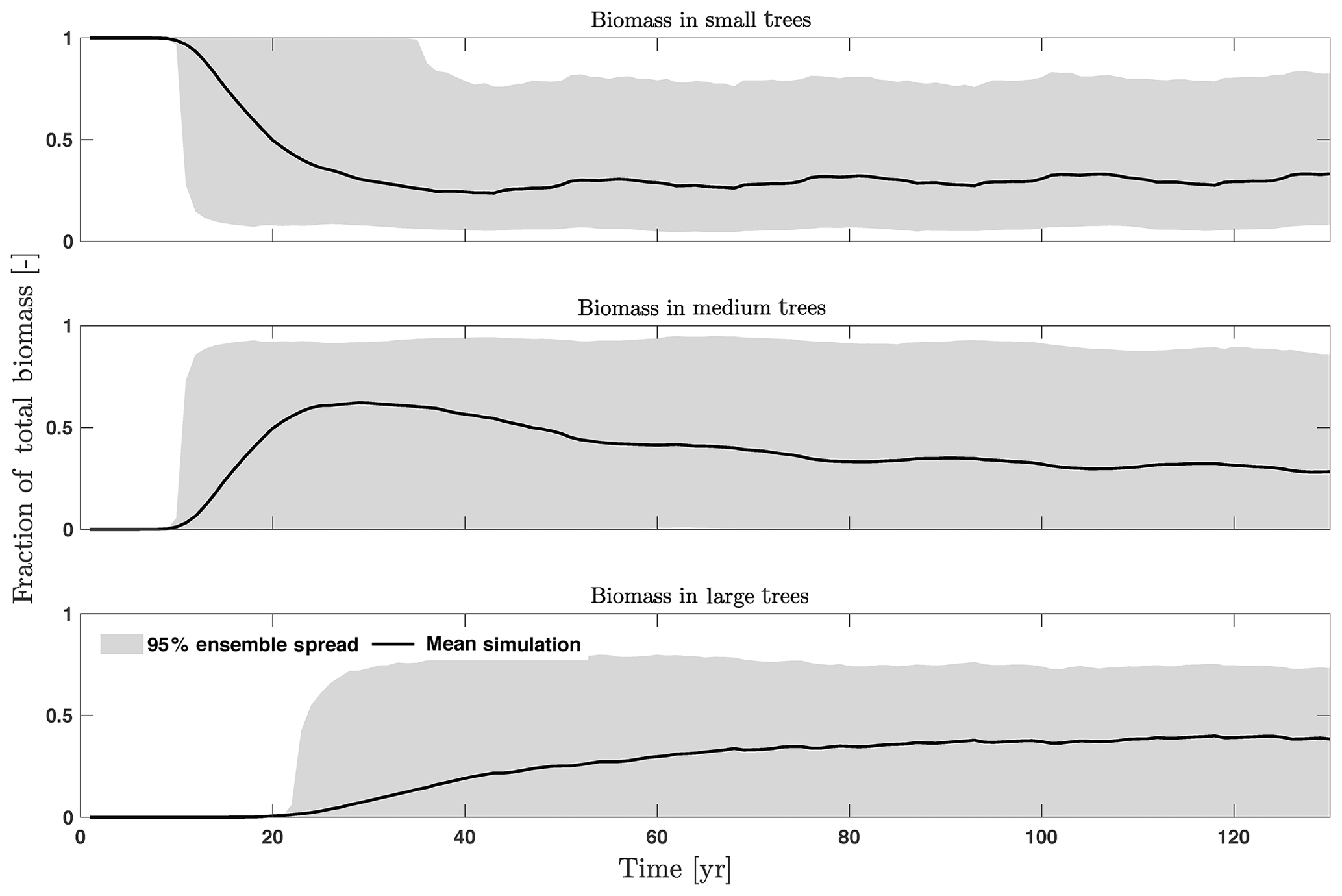
Figure D11Fraction of total biomass for trees of different sizes, including small (diameter <10 cm), medium (10 cm < diameter <50 cm), and large trees (diameter >50 cm).
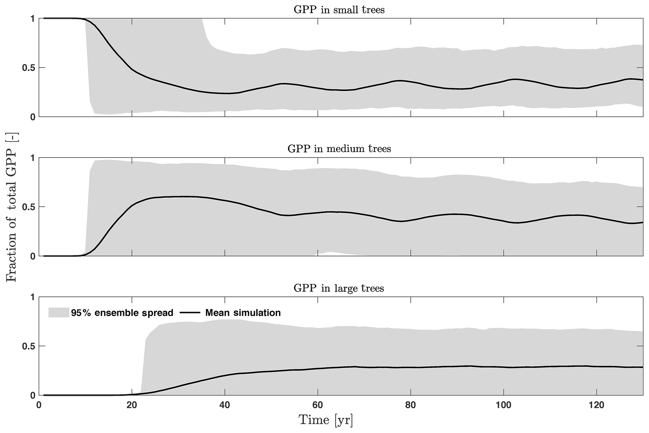
Figure D12Fraction of total GPP for trees of different sizes, including small (diameter <10 cm), medium (10 cm < diameter <50 cm), and large trees (diameter >50 cm).
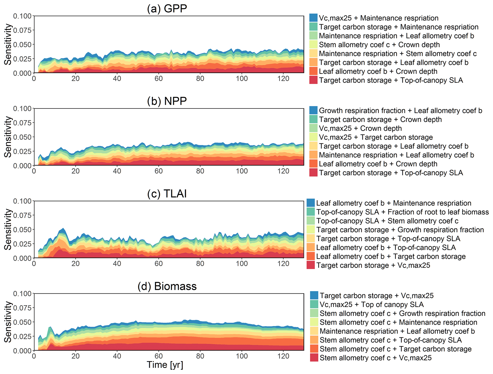
Figure D13Second-order sensitivity index of the model parameters for the GPP, NPP, LAI, and biomass outputs from CLM4.5(FATES). Shown are the top eight most important parameter interactions in order of importance based on the mean parametric sensitivity across years (red is the most important and blue is the least important).
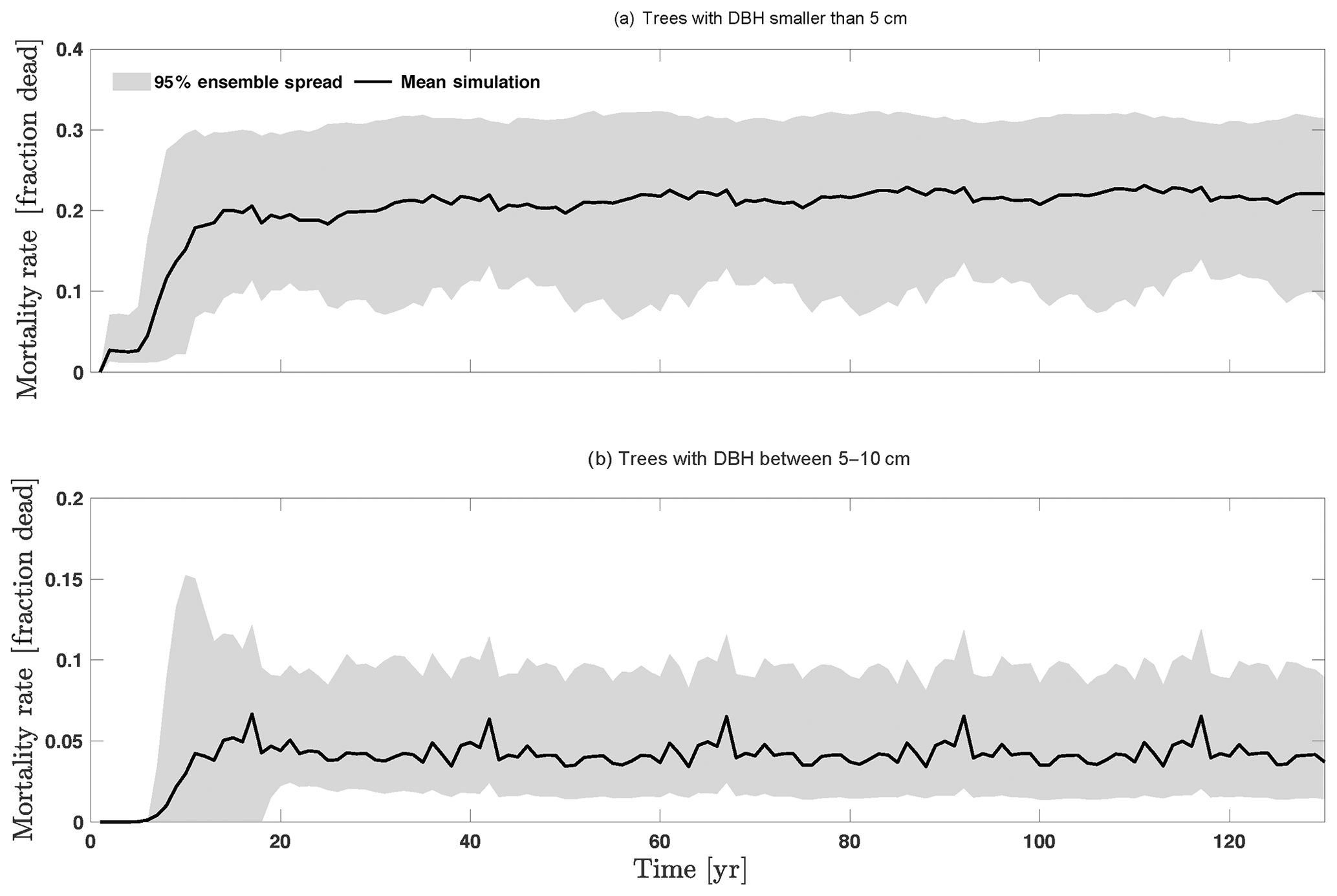
Figure D14Mortality outputs from CLM4.5(FATES) for trees with DBH smaller than 5 cm (a) and all trees with DBH between 5 and 10 cm (b). Shown is the 95 % (light grey) spread of the simulation ensemble, along with the mean simulation (black lines).
All authors contributed to the manuscript writing. CX designed the numerical experiments, developed scripts for sensitivity analysis, and analyzed model results; ECM implemented the model runs, extracted the model outputs, and analyzed model results; RAF, RGK, CDK, CX, and BOC contributed to the model development and simulations; JAH, DMR, SPS, and APW provided suggestions on sensitivity analysis, and LW provided support for model simulations; DJJ provide data on model evaluations; NGM, LMK, JQC, and JAV provided support and guidance on the experiment and manuscript.
The authors declare that they have no conflict of interest.
Model simulations were made possible thanks to the Conejo supercomputing system at the Los Alamos National Laboratory (LANL). We thank the four reviewers for their very helpful comments that substantially improved our manuscript.
This work was supported by the United States Department of Energy (US DOE) Office of Science Next Generation Ecosystem Experiment at Tropics (NGEE-T) project, the DOE Graduate Student Researcher (SCGSR) Fellowship, and the UC-Lab Fees Research Program (grant nos. 237285 and LFR-18-542511). Shawn P. Serbin was also partially supported by the United States Department of Energy contract no. DE-SC0012704 to Brookhaven National Laboratory. A portion of Elias C. Massoud's contribution to this research was carried out at the Jet Propulsion Laboratory, California Institute of Technology, under a contract with the National Aeronautics and Space Administration, Copyright 2019.
This paper was edited by Christoph Müller and reviewed by Xiangtao Xu, Nancy Kiang, and Sebastian Lienert.
Adams, H. R., Barnard, H. R., and Loomis, A. K.: Topography alters tree growth–climate relationships in a semi-arid forested catchment, Ecosphere, 5, 1–16, 2014. a
Ali, A. A., Xu, C., Rogers, A., Fisher, R. A., Wullschleger, S. D., Massoud, E. C., Vrugt, J. A., Muss, J. D., McDowell, N. G., Fisher, J. B., Reich, P. B., and Wilson, C. J.: A global scale mechanistic model of photosynthetic capacity (LUNA V1.0), Geosci. Model Dev., 9, 587–606, https://doi.org/10.5194/gmd-9-587-2016, 2016. a
Archer, G., Saltelli, A., and Sobol,I.: Sensitivity measures, anova-like techniques and the use of bootstrap, J. Stat. Comput. Simu., 58, 99–120,1997. a
Arora, V. K., Boer, G. J., Friedlingstein, P., Eby, M., Jones, C. D., Christian, J. R., Bonan, G., Bopp, L., Brovkin, V., Cadule, P., Brovkin, V., Cadule, P., and Hajima, T.: Carbon–concentration and carbon–climate feedbacks in cmip5 earth system models, J. Climate, 26 5289–5314, 2013. a, b
Bastidas, L. A., Gupta, H. V., Sorooshian, S., Shuttleworth, W. J., and Yang, Z. L.: Sensitivity analysis of a land surface scheme using multicriteria methods, J. Geophys. Res.-Atmos., 104, 19481–19490, 1999. a
Benton, T. G. and Grant, A.: Elasticity analysis as an important tool in evolutionary and population ecology Trends Ecol. Evol., 14, 467–471, 1999. a
Bonan, G. B., Lawrence, P. J., Oleson, K. W., Levis, S., Jung, M., Reichstein, M., Lawrence, D. M., and Swenson, S. C.: Improving canopy processes in the community land model version 4 (CLM4) using global flux fields empirically inferred from fluxnet data, J. Geophys. Res.-Biogeo., 116, G02014, https://doi.org/10.1029/2010JG001593, 2011. a
Campolongo, F., Saltelli, A., Sørensen, T. M., and Tarantola, S.: Hitchhiker's guide to sensitivity analysis, in: Sensitivity analysis, IEEE Computer Society Press, 15–47, 2000. a
Chave, J., Réjou-Méchain, M., Búrquez, A., Chidumayo, E., Colgan, M. S., Delitti, W. B., Duque, A., Eid, T., Fearnside, P. M., Goodman, R. C., and Henry, M.: Improved allometric models to estimate the aboveground biomass of tropical trees, Glob. Change Biol., 20, 3177–3190, 2014. a
Christoffersen, B. O., Gloor, M., Fauset, S., Fyllas, N. M., Galbraith, D. R., Baker, T. R., Kruijt, B., Rowland, L., Fisher, R. A., Binks, O. J., Sevanto, S., Xu, C., Jansen, S., Choat, B., Mencuccini, M., McDowell, N. G., and Meir, P.: Linking hydraulic traits to tropical forest function in a size-structured and trait-driven model (TFS v.1-Hydro), Geosci. Model Dev., 9, 4227–4255, https://doi.org/10.5194/gmd-9-4227-2016, 2016. a
Claussen, M., Mysak, L., Weaver, A., Crucifix, M., Fichefet, T., Loutre, M. F., Weber, S., Alcamo, J., Alexeev, V., Berger, A., and Calov, R.: Earth system models of intermediate complexity: closing the gap in the spectrum of climate system models, Clim. Dynam., 18, 579–586, 2002. a
Collalti, A., Thornton, P. E., Cescatti, A., Rita, A., Borghetti, M., Nole, A., Trotta, C., Ciais, P., and Matteucci, G.: The sensitivity of the forest carbon budget shifts across processes along with stand development and climate change, Ecol. Appl., 29, e01837, https://doi.org/10.1002/eap.1837, 2019. a, b, c
Collins, D. C. and Avissar, R.: An evaluation with the fourier amplitude sensitivity test (FAST) of which land-surface parameters are of greatest importance in atmospheric modeling, J. Climate, 7, 681–703, 1994. a
Cox, P. M., Betts, R. A., Jones, C. D., Spall, S. A., and Totterdell, I. J.: Acceleration of global warming due to carbon-cycle feedbacks in a coupled climate model, Nature, 408, 184–187, 2000. a, b
Crossley, J. F., Polcher, J., Cox, P. M., Gedney, N. and Planton, S.: Uncertainties linked to land-surface processes in climate change simulations, Clim. Dynam., 16, 949–961, 2000. a
Cukier, R., Fortuin, C., Shuler, K. E., Petschek, A., and Schaibly, J.: Study of the sensitivity of coupled reaction systems to uncertainties in rate coefficients. I theory, J. Chem. Phys., 59, 3873–3878, 1973. a
Da Rocha, H. R., Nobre, C. A., Bonatti, J. P., Wright, I. R., and Sellers, P. J.: A vegetation-atmosphere interaction study for amazonia deforestation using field data and a 'single column' model, Q. J. Roy. Meteor. Soc., 122, 567–594, 1996. a
Díaz, S., Kattge, J., Cornelissen, J. H., Wright, I. J., Lavorel, S., Dray, S., Reu, B., Kleyer, M., Wirth, C., Prentice, I. C., and Garnier, E.: The global spectrum of plant form and function, Nature, 529, 167–171, 2016. a
Dietze, M. C., Wolosin, M. S., and Clark, J. S.: Capturing diversity and interspecific variability in allometries: a hierarchical approach, Forest Ecol. Manage., 256, 1939–1948, 2008. a
Dietze, M. C., Serbin, S. P., Davidson, C., Desai, A. R., Feng, X., Kelly, R., Kooper, R., LeBauer, D., Mantooth, J., McHenry, K., and Wang, D.: A quantitative assessment of a terrestrial biosphere model's data needs across North American biomes, J. Geophys. Res.-Biogeo., 119, 286–300, 2014. a, b, c, d, e, f, g, h, i, j, k, l, m
Dunne, J. P., John, J. G., Adcroft, A. J., Griffies, S. M., Hallberg, R. W., Shevliakova, E., Stouffer, R. J., Cooke, W., Dunne, K. A., Harrison, M. J., and Krasting, J. P.: GFDL's ESM2 global coupled climate-carbon earth system models. part i: Physical formulation and baseline simulation characteristics, J. Climate, 25, 6646–6665, 2012. a
Dupuy, J. M. and Chazdon, R. L.: Effects of vegetation cover on seedling and sapling dynamics in secondary tropical wet forests in costa rica, J. Trop. Ecol., 22, 65–76, 2006. a
Entekhabi, D. and Eagleson, P. S.: Land surface hydrology parameterization for atmospheric general circulation models including subgrid scale spatial variability, J. Climate, 2, 816–831, 1989. a
Falster, D. S., Duursma, R. A., and FitzJohn, R. G.: How functional traits influence plant growth and shade tolerance across the life cycle, P. Natl. Acad. Sci. USA, 115, E6789–E6798, 2018. a, b
Farquhar, G. D.: Models of integrated photosynthesis of cells and leaves, Philos. T. Roy. Soc. B, 323, 357–367, https://doi.org/10.1098/rstb.1989.0016, 1989. a
Farrior, C. E., Bohlman, S. A., Hubbell, S., and Pacala, S. W.: Dominance of the suppressed: Power-law size structure in tropical forests, Science, 351, 155–157, 2016. a
Feldpausch, T. R., Banin, L., Phillips, O. L., Baker, T. R., Lewis, S. L., Quesada, C. A., Affum-Baffoe, K., Arets, E. J. M. M., Berry, N. J., Bird, M., Brondizio, E. S., de Camargo, P., Chave, J., Djagbletey, G., Domingues, T. F., Drescher, M., Fearnside, P. M., França, M. B., Fyllas, N. M., Lopez-Gonzalez, G., Hladik, A., Higuchi, N., Hunter, M. O., Iida, Y., Salim, K. A., Kassim, A. R., Keller, M., Kemp, J., King, D. A., Lovett, J. C., Marimon, B. S., Marimon-Junior, B. H., Lenza, E., Marshall, A. R., Metcalfe, D. J., Mitchard, E. T. A., Moran, E. F., Nelson, B. W., Nilus, R., Nogueira, E. M., Palace, M., Patiño, S., Peh, K. S.-H., Raventos, M. T., Reitsma, J. M., Saiz, G., Schrodt, F., Sonké, B., Taedoumg, H. E., Tan, S., White, L., Wöll, H., and Lloyd, J.: Height-diameter allometry of tropical forest trees, Biogeosciences, 8, 1081–1106, https://doi.org/10.5194/bg-8-1081-2011, 2011. a
Fisher, R., McDowell, N., Purves, D., Moorcroft, P., Sitch, S., Cox, P., Huntingford, C., Meir, P., and Woodward, F. I.: Assessing uncertainties in a second-generation dynamic vegetation model caused by ecological scale limitations, New Phytol., 187, 666–681, 2010. a, b, c, d
Fisher, R. A., Muszala, S., Verteinstein, M., Lawrence, P., Xu, C., McDowell, N. G., Knox, R. G., Koven, C., Holm, J., Rogers, B. M., Spessa, A., Lawrence, D., and Bonan, G.: Taking off the training wheels: the properties of a dynamic vegetation model without climate envelopes, CLM4.5(ED), Geosci. Model Dev., 8, 3593–3619, https://doi.org/10.5194/gmd-8-3593-2015, 2015. a, b, c, d, e, f, g, h
Fisher, R. A., Koven, C. D., Anderegg, W. R., Christoffersen, B. O., Dietze, M. C., Farrior, C. E., Holm, J. A., Hurtt, G. C., Knox, R. G., Lawrence, P. J., and Lichstein, J. W.: Vegetation demographics in earth system models: A review of progress and priorities, Glob. Change Biol., 24, 35–54, 2018. a, b, c
Foley, J. A., Prentice, I. C., Ramankutty, N., Levis, S., Pollard, D., Sitch, S., and Haxeltine, A.: An integrated biosphere model of land surface processes, terrestrial carbon balance, and vegetation dynamics, Global Biogeochem. Cy., 10, 603–628, 1996. a
Francos, A., Elorza, F. J., Bouraoui, F., Bidoglio, G., and Galbiati, L.: Sensitivity analysis of distributed environmental simulation models: understanding the model behaviour in hydrological studies at the catchment scale, Reliab. Eng. Syst. Safe., 79, 205–218, 2003. a
Friedlingstein, P., Cox, P., Betts, R., Bopp, L., von Bloh, W., Brovkin, V., Cadule, P., Doney, S., Eby, M., Fung, I., and Bala, G.: Climate-carbon cycle feedback analysis: Results from the C4MIP model intercomparison, J. Climate, 19, 3337–3353, 2006. a
Geromel, J. C.: Optimal linear filtering under parameter uncertainty, IEEE T. Signal Proces., 47, 168–175, 1999. a
Golaz, J. C., Caldwell, P. M., Van Roekel, L. P., Petersen, M. R., Tang, Q., Wolfe, J. D., Abeshu, G., Anantharaj, V., Asay-Davis, X. S., Bader, D. C., Baldwin, S. A., Bisht, G., Bogenschutz, P. A., Branstetter, M., Brunke, M. A., Brus, S. R., Burrows, S. M., Cameron-Smith, P. J., Donahue, A. S., Deakin, M., Easter, R. C., Evans, K. J., Feng, Y., Flanner, M., Foucar, J. G., Fyke, J. G., Griffin, B. M., Hannay, C., Harrop, B. E., Hoffman, M. J., Hunke, E. C., Jacob, R. L., Jacobsen, D. W., Jeffery, N., Jones, P. W., Keen, N. D., Klein, S. A., Larson, V. E., Leung, L. R., Li, H.-Y., Lin, W., Lipscomb, W. H., Ma, P.-L., Mahajan, S., Maltrud, M. E., Mametjanov, A., McClean, J. L., McCoy, R. B., Neale, R. B., Price, S. F., Qian, Y., Rasch, P. J., Reeves Eyre, J. E. J., Riley, W. J., Ringler, T. D., Roberts, A. F., Roesler, E. L., Salinger, A. G., Shaheen, Z., Shi, X., Singh, B., Tang, J., Taylor, M. A., Thornton, P. E., Turner, A. K., Veneziani, M., Wan, H., Wang, H., Wang, S., Williams, D. N., Wolfram, P. J., Worley, P. H., Xie, S., Yang, Y., Yoon, J.H., Zelinka, M. D., Zender, C. S., Zeng, X., Zhang, C., Zhang, K., Zhang, Y., Zheng, X., Zhou, T., and Zhu, Q.: The DOE E3SM coupled model version 1: Overview and evaluation at standard resolution, J. Adv. Model. Earth Sy., 11, 2089–2129, https://doi.org/10.1029/2018MS001603, 2019. a
Groenendijk, M., Dolman, A. J., Van Der Molen, M. K., Leuning, R., Arneth, A., Delpierre, N., Gash, J. H. C., Lindroth, A., Richardson, A. D., Verbeeck, H., and Wohlfahrt, G.: Assessing parameter variability in a photosynthesis model within and between plant functional types using global Fluxnet eddy covariance data, Agr. Forest Meteorol., 151, 22–38, 2011. a
Gupta, H. V., Bastidas, L. A., Sorooshian, S., Shuttleworth, W. J., and Yang, Z. L.: Parameter estimation of a land surface scheme using multicriteria methods, J. Geophys. Res.-Atmos., 104, 19491–19503, 1999. a
Haaker, M., and Verheijen, P.:, Local and global sensitivity analysis for a reactor design with parameter uncertainty, Chem. Eng. Res. Des., 82, 591–598, 2004. a
Helton, J. C.: Uncertainty and sensitivity analysis techniques for use in performance assessment for radioactive waste disposal, Reliab. Eng. Syst. Safe., 42, 327–367, 1993. a
Hickler, T., Smith, B., Sykes, M. T., Davis, M. B., Sugita, S., and Walker, K.: Using a generalized vegetation model to simulate vegetation dynamics in northeastern USA, Ecology, 85, 519–530, 2004. a, b
Holm, J. A., Knox, R. G., Zhu, Q., Fisher, R. A., Koven, C. D., Lima, A. J. N., Riley, W. J., Longo, M., Negron-Juarez, R. I., de Araujo, A. C., Manzi, A., Kueppers, L. M., Moorcroft, P. R., Higuchi, N., and Chambers, J. Q.: The Central Amazon forest sink under current and future atmospheric CO2: Predictions from big-leaf and demographic vegetation models, J. Geophys. Res., in review, 2019. a
Hunter, M. O., Keller, M., Victoria, D., and Morton, D. C.: Tree height and tropical forest biomass estimation, Biogeosciences, 10, 8385–8399, https://doi.org/10.5194/bg-10-8385-2013, 2013. a, b
Hurrell, J. W., Holland, M. M., Gent, P. R., Ghan, S., Kay, J. E., Kushner, P. J., Lamarque, J. F., Large, W. G., Lawrence, D., Lindsay, K., and Lipscomb, W. H.: The community earth system model: a framework for collaborative research, B. Am. Meteorol. Soc., 94, 1339–1360, 2013. a
Johnson, D. J., Needham, J., Xu, C., Massoud, E. C., Davies, S. J., Anderson-Teixeira, K. J., Bunyavejchewin, S., Chambers, J. Q., Chang-Yang, C. H., Chiang, J. M., and Chuyong, G. B.: Climate sensitive size-dependent survival in tropical trees, Nature Ecology and Evolution, 2, 1436–1442, 2018. a
Jung, M., Reichstein, M., and Bondeau, A.: Towards global empirical upscaling of FLUXNET eddy covariance observations: validation of a model tree ensemble approach using a biosphere model, Biogeosciences, 6, 2001–2013, https://doi.org/10.5194/bg-6-2001-2009, 2009. a
Kattge, J., Diaz, S., Lavorel, S., Prentice, I. C., Leadley, P., Bönisch, G., Garnier, E., Westoby, M., Reich, P. B., Wright, I. J., and Cornelissen, J. H. C.: TRY – a global database of plant traits, Glob. Change Biol., 17, 2905–2935, 2011. a
Kattge, J., Ogle, K., Bönisch, G., Díaz, S., Lavorel, S., Madin, J., Nadrowski, K., Nöllert, S., Sartor, K., and Wirth, C.: A generic structure for plant trait databases, Methods Ecol. Evol., 2, 202–213, 2011. a
Kioutsioukis, I., Tarantola, S., Saltelli, A., and Gatelli, D.: Uncertainty and global sensitivity analysis of road transport emission estimates, Atmos. Environ., 38, 6609–6620, 2004. a
Kitanidis, P. K.: Parameter uncertainty in estimation of spatial functions: Bayesian analysis, Water Resour. Res., 22, 499–507, 1986. a
Knyazikhin, Y., Glassy, J., Privette, J. L., Tian, Y., Lotsch, A., Zhang, Y., Wang, Y., Morisette, J. T., Votava, P., Myneni, R. B., Nemani, R. R., and Running, S. W.: MODIS leaf area index (LAI) and fraction of photosynthetically active radiation absorbed by vegetation (FPAR) product (MOD15) algorithm theoretical basis document, Theoretical Basis Document, NASA Goddard Space Flight Center, Greenbelt, MD, 20771, 1999. a
Krinner, G., Viovy, N., de Noblet-Ducoudré, N., Ogée, J., Polcher, J., Friedlingstein, P., Ciais, P., Sitch, S., and Prentice, I. C.: A dynamic global vegetation model for studies of the coupled atmosphere-biosphere system, Global Biogeochem. Cy., 19, GB1015, https://doi.org/10.1029/2003GB002199, 2005. a
Kumar, S. V., Peters-Lidard, C. D., Tian, Y., Houser, P. R., Geiger, J., Olden, S., Lighty, L., Eastman, J. L., Doty, B., Dirmeyer, P., and Adams, J.: Land information system: An interoperable framework for high resolution land surface modeling, Environ. Modell. Softw., 21, 1402–1415, 2006. a
Lawrence, D. M., Oleson, K. W., Flanner, M. G., Thornton, P. E., Swenson, S. C., Lawrence, P. J., Zeng, X., Yang, Z. L., Levis, S., Sakaguchi, K., and Bonan, G. B.: Parameterization improvements and functional and structural advances in version 4 of the Community Land Model, J. Adv. Model Earth Sy., 3, https://doi.org/10.1029/2011MS00045, 2012. a
LeBauer, D. S., Wang, D., Richter, K. T., Davidson, C. C., and Dietze, M. C.: Facilitating feedbacks between field measurements and ecosystem models, Ecol. Monogr., 83, 133–154, 2013. a, b, c, d, e, f
Leuning, R.: Temperature dependence of two parameters in a photosynthesis model, Plant Cell Environ., 25, 1205–1210, 2002. a, b
Lieberman, D., Lieberman, M., Hartshorn, G., and Peralta, R.: Growth rates and age-size relationships of tropical wet forest trees in costa rica, J. Trop. Ecol., 1, 97–109, 1985. a
Lu, Y. and Mohanty, S.: Sensitivity analysis of a complex, proposed geologic waste disposal system using the fourier amplitude sensitivity test method, Reliab. Eng. Syst. Safe., 72, 275–291, 2001. a
Masson, V., Champeaux, J. L., Chauvin, F., Meriguet, C., and Lacaze, R.: A global database of land surface parameters at 1-km resolution in meteorological and climate models, J. Climate, 16, 1261–1282, 2003. a, b
Massoud, E. C., Purdy, A. J., Christoffersen, B. O., Santiago, L. S., and Xu, C.: Bayesian inference of hydraulic properties in and around a white fir using a process-based ecohydrologic model, Environ. Modell. Softw., 115, 76–85, 2019a. a
Massoud, E., Xu, C., Fisher, R., Knox, R., Walker, A., Serbin, S., Christoffersen, B., Holm, J., Kueppers, L., Ricciuto, D., Wei, L., Johnson, D., Chambers, J., Koven, C., McDowell, N., and Vrugt, J.: Identification of key parameters controlling demographically structured vegetation dynamics in a Land Surface Model, 1.0, NGEE Tropics Data Collection, (dataset), https://doi.org/10.15486/ngt/1497413, 2019b. a
McDowell, N. G., Williams, A. P., Xu, C., Pockman, W. T., Dickman, L. T., Sevanto, S., Pangle, R., Limousin, J., Plaut, J., Mackay, D. S., and Ogee, J.: Multi-scale predictions of massive conifer mortality due to chronic temperature rise, Nat. Clim. Change, 6, 295–300, 2016. a
McDowell, N., Allen, C. D., Anderson–Teixeira, K., Brando, P., Brienen, R., Chambers, J., Christoffersen, B., Davies, S., Doughty, C., Duque, A., Espirito–Santo, F., Fisher, R., Fontes, C. G., Galbraith, D., Goodsman, D., Grossiord, C., Hartmann, H., Holm, J., Johnson, D. J., Kassim, A. R., Keller, M., Koven, C., Kueppers, L., Kumagai, T., Malhi, Y., McMahon, S. M., Mencuccini, M., Meir, P., Moorcroft, P., Muller–Landau, H. C., Phillips, O. L., Powell, T., Sierra, C. A., Sperry, J., Warren, J., Xu, C., and Xu, X.: Drivers and mechanisms of tree mortality in moist tropical forests, New Phytol., 219, 851–869, 2018. a
McRae, G. J., Tilden, J. W., and Seinfeld, J. H.: Global sensitivity analysis – a computational implementation of the Fourier Amplitude Sensitivity Test (FAST), Comput. Chem. Eng., 6, 15–25, 1982. a
Menberg, K., Heo, Y., and Choudhary, R.: Sensitivity analysis methods for building energy models: Comparing computational costs and extractable information, Energy Buildings, 133, 433–445, 2016. a
Moorcroft, P. R., Hurtt, G., and Pacala, S. W.: A method for scaling vegetation dynamics: the ecosystem demography model (ED), Ecol. Monogr., 71, 557–586, 2001. a, b
Noilhan, J. and Planton, S.: A simple parameterization of land surface processes for meteorological models, Mon. Weather Rev., 117, 536–549, 1989. a
O'Hagan, A., and Leonard, T.: Bayes estimation subject to uncertainty about parameter constraints, Biometrika, 63, 201–203, 1976. a
Oleson, K. W., Lawrence, D. M., Bonan, G. B., Drewniak, B., Huang, M., Koven, C. D., Levis, S., Li, F., Riley, W. J., Subin, Z., Swenson, S. C., and Thornton, P. E.: Technical description of version 4.5 of the Community Land Model (CLM), NCAR Technical Note NCAR/TN-503+STR, 420 pp., https://doi.org/10.5065/D6RR1W7M, 2013. a
Pan, Y., McGuire, A. D., Melillo, J. M., Kicklighter, D. W., Sitch, S., and Prentice, I. C.: A biogeochemistry-based dynamic vegetation model and its application along a moisture gradient in the continental united states, J. Veg. Sci., 13, 369–382, 2002. a
Pappas, C., Fatichi, S., Leuzinger, S., Wolf, A., and Burlando, P.: Sensitivity analysis of a process-based ecosystem model: Pinpointing parameterization and structural issues, J. Geophys. Res.-Biogeo., 118, 505–528, https://doi.org/10.1002/jgrg.20035, 2013. a, b, c, d, e, f, g, h, i
Qian, T., Dai, A., Trenberth, K. E., and Oleson, K. W.: Simulation of global land surface conditions from 1948 to 2004. Part I: Forcing data and evaluations, J. Hydrometeorol., 7, 953–975, 2006. a, b
Razavi, S. and Gupta, H. V.: A new framework for comprehensive, robust, and efficient global sensitivity analysis: 1. theory, Water Resour. Res., 52, 423–439, 2016. a
Rogers, A.: The use and misuse of Vc,max in Earth System Models, Photosynth. Res., 119, 15–29, 2014. a
Rogers, A., Medlyn, B. E., Dukes, J. S., Bonan, G., Caemmerer, S., Dietze, M. C., Kattge, J., Leakey, A. D., Mercado, L. M., Niinemets, Ü., and Prentice, I. C.: A roadmap for improving the representation of photosynthesis in earth system models, New Phytol., 213, 22–42, 2017. a
Rosolem, R., Gupta, H. V., Shuttleworth, W. J., de Gonçalves, L. G. G., and Zeng, X.: Towards a comprehensive approach to parameter estimation in land surface parameterization schemes, Hydrol. Process., 27, 2075–2097, 2013. a
Ruppert, D., Wand, M. P., and Carroll, R. J.:Semiparametric regression, Cambridge university press, 2003. a
Saltelli, A., Tarantola, S., and Chan, K. S.: A quantitative model-independent method for global sensitivity analysis of model output, Technometrics, 41, 39–56, 1999. a
Saltelli, A., Chan, K., and Scott, E. M.: Sensitivity analysis, vol. 1, Wiley New York, 2000. a, b
Sargsyan, K., Safta, C., Najm, H. N., Debusschere, B. J., Ricciuto, D., and Thornton, P.: Dimensionality reduction for complex models via bayesian compressive sensing, Int. J. Uncertain. Quan., 4, 63–93, 2014. a, b, c, d
Sato, H., Itoh, A., and Kohyama, T.: SEIB–DGVM: A new dynamic global vegetation model using a spatially explicit individual-based approach, Ecol. Model., 200, 279–307, 2007. a
Scheiter, S., Langan, L., and Higgins, S. I.: Next-generation dynamic global vegetation models: learning from community ecology, New Phytol., 198, 957–969, 2013. a
Schwalm, C. R., Williams, C. A., Schaefer, K., Anderson, R., Arain, M. A., Baker, I., Barr, A., Black, T. A., Chen, G., Chen, J. M., and Ciais, P.: A model-data intercomparison of CO2 exchange across North America: Results from the North American carbon program site synthesis, J. Geophys. Res.-Biogeo., 115, G00H05, https://doi.org/10.1029/2009JG001229, 2010. a
Sen, O. L., Bastidas, L. A., Shuttleworth, W. J., Yang, Z. L., Gupta, H. V., and Sorooshian, S.: Impact of field-calibrated vegetation parameters on gcm climate simulations, Q. J. Roy. Meteorol. Soc., 127, 1199–1223, 2001. a
Sitch, S., Smith, B., Prentice, I. C., Arneth, A., Bondeau, A., Cramer, W., Kaplan, J. O., Levis, S., Lucht, W., Sykes, M. T., and Thonicke, K.: Evaluation of ecosystem dynamics, plant geography and terrestrial carbon cycling in the LPJ dynamic global vegetation model, Glob. Change Biol., 9, 161–185, 2003. a
Sitch, S., Huntingford, C., Gedney, N., Levy, P. E., Lomas, M., Piao, S. L., Betts, R., Ciais, P., Cox, P., Friedlingstein, P., and Jones, C. D.: Evaluation of the terrestrial carbon cycle, future plant geography and climate-carbon cycle feedbacks using five dynamic global vegetation models (DGVMs), Glob. Change Biol., 14, 2015–2039, 2008. a
Sobol', I.M.: On sensitivity estimation for nonlinear mathematical models, Matematicheskoe Modelirovanie, 2, 112–118, 1990. a, b, c
Song, X. M., Zhang, J. Y., Zhan, C. S., Xuan, Y. Q., Ye, M., and Xu, C. G.: Global sensitivity analysis in hydrological modeling: Review of concepts, methods, theoretical framework, and applications, J. Hydrol., 523, 739–757, 2015. a
Sudret, B.: Global sensitivity analysis using polynomial chaos expansions, Reliab. Eng. Syst. Safe., 93, 964–979, 2008. a, b
Thonicke, K., Venevsky, S., Sitch, S., and Cramer, W.: The role of fire disturbance for global vegetation dynamics: coupling fire into a dynamic global vegetation model, Global Ecol. Biogeogr., 10, 661–677, 2001. a
Vrugt, J., Wijk, M. V., Hopmans, J. W., and Šimunek, J.: One-, two-, and three-dimensional root water uptake functions for transient modeling, Water Resour. Res., 37, 2457–2470, 2001. a
Wahba, G.: Spline models for observational data, SIAM, ISBN: 978-0-89871-244-5, 161 pp., https://doi.org/10.1137/1.9781611970128, 1990. a
Wang, G., Gertner, G., Liu, X., and Anderson, A.: Uncertainty assessment of soil erodibility factor for revised universal soil loss equation, Catena, 46, 1–14, 2001. a
Wang, J., Li, X., Lu, L., and Fang, F.: Parameter sensitivity analysis of crop growth models based on the extended Fourier amplitude sensitivity test method, Environ. Modell. Softw., 48, 171–182, 2013. a, b, c, d, e, f
Waring, R., Landsberg, J., and Williams, M.: Net primary production of forests: a constant fraction of gross primary production?, Tree Physiol., 18, 129–134, 1998. a
Waring, R. H. and Running, S. W.:Forest ecosystems: analysis at multiple scales, Elsevier, 2010. a
Wood, E. F., Lettenmaier, D. P., and Zartarian, V. G.: A land-surface hydrology parameterization with subgrid variability for general circulation models, J. Geophys. Res.-Atmos., 97, 2717–2728, 1992. a
Worbes, M.: Annual growth rings, rainfall-dependent growth and long-term growth patterns of tropical trees from the caparo forest reserve in venezuela, J. Ecol., 87, 391–403, 1999. a
Xu, C. and Gertner, G. Z.: Extending a global sensitivity analysis technique to models with correlated parameters, Comput. Stat. Data An., 51, 5579–5590, 2007. a
Xu, C. and Gertner, G. Z.: Uncertainty and sensitivity analysis for models with correlated parameters, Reliab. Eng. Syst. Safe., 93, 1563–1573, 2008. a
Xu, C. and Gertner, G. Z.: Uncertainty analysis of transient population dynamics, Ecol. Model., 220, 283–293, 2009. a, b, c
Xu, C. and Gertner, G. Z.: Understanding and comparisons of different sampling approaches for the fourier amplitudes sensitivity test (FAST), Comput. Stat. Data An., 55, 184–198, 2011. a, b, c, d, e
Xu, C. and Gertner, G. Z.: Reliability of global sensitivity indices, J. Stat. Comput. Sim., 81, 1939–1969, 2011. a
Xu, C., Gertner, G. Z., and Scheller, R. M.: Uncertainties in the response of a forest landscape to global climatic change, Glob. Change Biol., 15, 116–131, 2009. a, b
Xu, C., Legros, M., Gould, F., and Lloyd, A. L.: Understanding uncertainties in model-based predictions of Aedes aegypti population dynamics, PLoS Neglect. Trop. D., 4, e830, https://doi.org/10.1371/journal.pntd.0000830, 2010. a
Xu, C., McDowell, N. G., Sevanto, S., and Fisher, R. A.: Our limited ability to predict vegetation dynamics under water stress, New Phytol., 200, 298–300, 2013. a
Zaehle, S., Sitch, S., Smith, B., and Hatterman, F.: Effects of parameter uncertainties on the modeling of terrestrial biosphere dynamics, Global Biogeochem. Cy., 19, GB3020, https://doi.org/10.1029/2004GB002395, 2005. a
Zeng, X.: Global vegetation root distribution for land modeling, J. Hydrometeorol., 2, 525–530, 2001. a
Zhou, X., Lin, H., and Lin, H.: Global Sensitivity Analysis, in: Encyclopedia of GIS, 408–409, 2008. a
- Abstract
- Introduction
- Materials and methods
- Results
- Discussion
- Conclusions
- Code and data availability
- Appendix A: Allometry equations
- Appendix B: Temperature response curve
- Appendix C: Carbon storage in CLM4.5(FATES)
- Appendix D: Appendix figures and tables
- Author contributions
- Competing interests
- Acknowledgements
- Financial support
- Review statement
- References